Embed Size (px)
Citation preview

Introduction to Artificial Neural Networks
Dynerowicz Seweryn
Facultes Universitaires Notre-Dame de la Paix
27 March 2007
Dynerowicz Seweryn Introduction to Artificial Neural Networks

Outline
1 Introduction
2 FundamentalsBiological neuronArtificial neuronArtificial Neural Network
Dynerowicz Seweryn Introduction to Artificial Neural Networks

Outline
3 Single-layer ANNPerceptronAdalineLimitations
4 Multi-layer ANNTopologyGeneralised Delta RuleDeficiencies
5 Recurrent ANNJordan NetworkHopfield Network
Dynerowicz Seweryn Introduction to Artificial Neural Networks
Outline
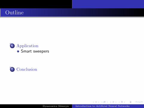
6 ApplicationSmart sweepers
7 Conclusion
Dynerowicz Seweryn Introduction to Artificial Neural Networks

IntroductionFundamentals
1 Introduction
2 FundamentalsBiological neuronArtificial neuronArtificial Neural Network
Dynerowicz Seweryn Introduction to Artificial Neural Networks

IntroductionFundamentals
History
1943 : W. McCulloch & W. Pitts : first model of artificialneuron
1949 : D. Hebb describes the first learning rule (Hebb’s Law)
1957 : F. Rosenblatt designs the Perceptron
1965 : Nils J. Nilsson publishes ”Learning Machines”(automated learning fundamentals)
Dynerowicz Seweryn Introduction to Artificial Neural Networks

IntroductionFundamentals
History
1969 : M. Minsky & S. Papert expose limitations ofPerceptron (XOR problem)
1975 : First multi-layer ANN with training algorithm(Cognitron)
1982 : Hopfield networks (J. Hopfield), Self-Organizing Map(T. Kohonen)
1986 : Backpropagation algorithm (R. Williams, D. Rumelhart& G. Hinton)
Dynerowicz Seweryn Introduction to Artificial Neural Networks
IntroductionFundamentals
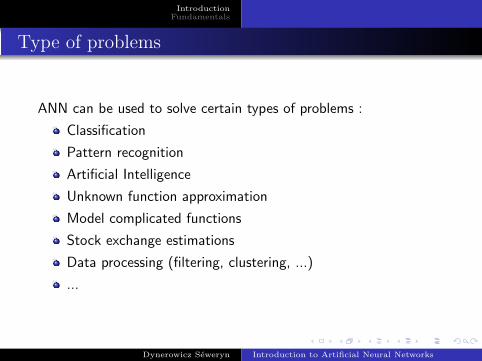
Type of problems
ANN can be used to solve certain types of problems :
Classification
Pattern recognition
Artificial Intelligence
Unknown function approximation
Model complicated functions
Stock exchange estimations
Data processing (filtering, clustering, ...)
...
Dynerowicz Seweryn Introduction to Artificial Neural Networks

IntroductionFundamentals
Biological neuronArtificial neuronArtificial Neural Network
1 Introduction
2 FundamentalsBiological neuronArtificial neuronArtificial Neural Network
Dynerowicz Seweryn Introduction to Artificial Neural Networks

IntroductionFundamentals
Biological neuronArtificial neuronArtificial Neural Network
A view of the biological neuron
The human nervous system is composed of about 1011
neurons.
The synapses are the connections between axon terminals anddendrites.
The synapses are characterized by a level of effectiveness.
Dynerowicz Seweryn Introduction to Artificial Neural Networks

IntroductionFundamentals
Biological neuronArtificial neuronArtificial Neural Network
A view of the biological neuron
The impulses received at each dendrites are summed together.
If the sum is above the stimulation threshold, the nucleusemits a spike down the axon.
Dynerowicz Seweryn Introduction to Artificial Neural Networks
IntroductionFundamentals
Biological neuronArtificial neuronArtificial Neural Network
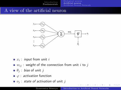
A view of the artificial neuron
xi : input from unit i
wij : weight of the connection from unit i to j
θj : bias of unit j
ϕ : activation function
oj : state of activation of unit j
Dynerowicz Seweryn Introduction to Artificial Neural Networks
IntroductionFundamentals
Biological neuronArtificial neuronArtificial Neural Network
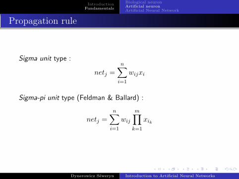
Propagation rule
Sigma unit type :
netj =n∑
i=1
wijxi
Sigma-pi unit type (Feldman & Ballard) :
netj =n∑
i=1
wij
m∏k=1
xik
Dynerowicz Seweryn Introduction to Artificial Neural Networks

IntroductionFundamentals
Biological neuronArtificial neuronArtificial Neural Network
Activation function
Threshold function (Heaviside or sgn) :
ϕ(v) ={
1 if v ≥ 00 if v < 0
Semi-linear function :
ϕ(v) =
1 if v ≥ 1
2v if − 1
2 < v < 12
0 if v ≤ −12
Sigmoid function :
ϕ(v) =1
1 + e−kv
Dynerowicz Seweryn Introduction to Artificial Neural Networks

IntroductionFundamentals
Biological neuronArtificial neuronArtificial Neural Network
Topology
Separation can be made between two types of ANN structure :
Feed-forward : acyclic and layer-decomposable graph(Perceptron, Adaline)
Recurrent (Jordan, Hopfield, Kohonen)
Dynerowicz Seweryn Introduction to Artificial Neural Networks

IntroductionFundamentals
Biological neuronArtificial neuronArtificial Neural Network
What is an ANN ?
ANN : I ⇒ O
I : set of inputs
O : set of outputs
Initially, the ANN will not respond correctly to given inputs.
Because
{weightsbiases
}are not adapted.
Dynerowicz Seweryn Introduction to Artificial Neural Networks

IntroductionFundamentals
Biological neuronArtificial neuronArtificial Neural Network
How does an ANN learns ?
Most interesting characteristic of ANN is the capacity to generalizeinformation from samples.
This generalisation occurs through the learning process.
Main idea : successive weight adjustment (gradient descentmethod)
Supervised learning (or Associative learning)
Unsupervised learning (or Self-organisation)
Dynerowicz Seweryn Introduction to Artificial Neural Networks

IntroductionFundamentals
Biological neuronArtificial neuronArtificial Neural Network
Supervised learning
Idea :
generate a population of input-output pairs
feed ANN with input
re-adjust weights and biases if the ANN doesn’t output whatis expected
Representation of data is imposed to the ANN
Dynerowicz Seweryn Introduction to Artificial Neural Networks

IntroductionFundamentals
Biological neuronArtificial neuronArtificial Neural Network
Unsupervised learning
Idea :
generate a population of input pairs
feed the population to the ANN
let it extract statistical properties from the population
Representation of data is defined by the ANN
Dynerowicz Seweryn Introduction to Artificial Neural Networks

IntroductionFundamentals
Biological neuronArtificial neuronArtificial Neural Network
Hebbian Learning Rule
wij = wij + δwij
δwij = γoioj
with :
wij : weight from unit i to unit j
γ : learning rate
oi : state of activation of unit i
Virtually, all learning rules can be considered as variants of HLR.
Dynerowicz Seweryn Introduction to Artificial Neural Networks

IntroductionFundamentals
Biological neuronArtificial neuronArtificial Neural Network
Learning Rate
Defines the speed at which the ANN will learn
Usually a constant
0 < γ ≤ 1
γ → 0 : slow convergence but stable solution.
γ → 1 : fast convergence but instable solution.
Dynerowicz Seweryn Introduction to Artificial Neural Networks

IntroductionFundamentals
Biological neuronArtificial neuronArtificial Neural Network
Over-fitting
Excessive learning or inadapted training set can lead to an”over-fitted” network.
An over-fitted ANN is specialised for the set which was used totrain it.
It lost a great part of its generalisation capability.
Dynerowicz Seweryn Introduction to Artificial Neural Networks

IntroductionFundamentals
Biological neuronArtificial neuronArtificial Neural Network
Two issues
Representational power : ability of an ANN to represent adesired function. Since an ANN is built from standardfunctions, it can only approximate the desired function, evenfor an optimal set of weights. Ergo, the approximation errorcan never be equal to 0.
Learning algorithm : given there exists a set of optimalweights (i.e. which minimize the approximation error), is therea procedure to compute them ?
Dynerowicz Seweryn Introduction to Artificial Neural Networks

Single-layer ANNMulti-layer ANNRecurrent ANN
PerceptronAdalineLimitations
3 Single-layer ANNPerceptronAdalineLimitations
4 Multi-layer ANNTopologyGeneralised Delta RuleDeficiencies
5 Recurrent ANNJordan NetworkHopfield Network
Dynerowicz Seweryn Introduction to Artificial Neural Networks
Single-layer ANNMulti-layer ANNRecurrent ANN
PerceptronAdalineLimitations
Perceptron
Proposed by F. Rosenblatt in 1957.
A Perceptron is a single-layer ANN.
Composed of one or more output neurons, connected to all inputs.
Typically used as a linear classifier.
Dynerowicz Seweryn Introduction to Artificial Neural Networks

Single-layer ANNMulti-layer ANNRecurrent ANN
PerceptronAdalineLimitations
Simple case
Consider the following Perceptron :
1 neuron
2 inputs
1 output
Threshold-type activation function :
ϕ(v) ={
1 if v > 0−1 otherwise
We can use it as a classifier with a separation line :
w1x1 + w2x2 + θ = 0
Dynerowicz Seweryn Introduction to Artificial Neural Networks

Single-layer ANNMulti-layer ANNRecurrent ANN
PerceptronAdalineLimitations
Simple case
x2 = −w1
w2x1 −
θ
w2
Dynerowicz Seweryn Introduction to Artificial Neural Networks

Single-layer ANNMulti-layer ANNRecurrent ANN
PerceptronAdalineLimitations
Perceptron learning
Learning consists of a successive weight adjustment :
wij = wij + ∆wij
θj = θj + ∆θj
Problem : how to compute the ∆wij and ∆θj ?
Dynerowicz Seweryn Introduction to Artificial Neural Networks

Single-layer ANNMulti-layer ANNRecurrent ANN
PerceptronAdalineLimitations
Perceptron Learning Rule
Consider a set of learning samples (x, d(x)), with :
x : input vector
d(x) : desired output
Learning Method :
1. Start with random weights for the connections;
2. Select an input vector x from the set of training samples;
3. If o 6= d(x) (the perceptron gives an incorrect response),modify all connections wij according to :
∆wij = dj(x)xi
∆θj = dj(x)
4. Go back to 2.
Dynerowicz Seweryn Introduction to Artificial Neural Networks
Single-layer ANNMulti-layer ANNRecurrent ANN
PerceptronAdalineLimitations
Convergence Theorem
Theorem 1. If there exists a set of connection weights w∗ whichis able to perform the transformation o = d(x), the perceptronlearning rule will converge to some solution (which may or may notbe the same as w∗) in a finite number of steps for any initialchoice of the weights.
Dynerowicz Seweryn Introduction to Artificial Neural Networks

Single-layer ANNMulti-layer ANNRecurrent ANN
PerceptronAdalineLimitations
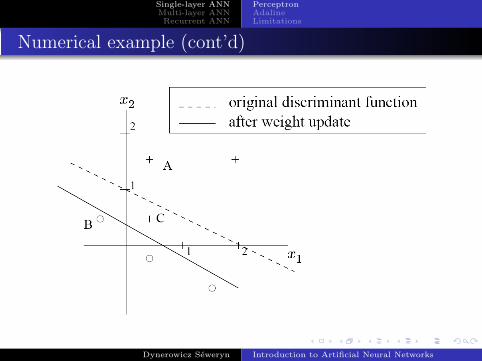
Numerical example
Initial parameters :
w1 = 1w2 = 2θ = −2
Set of samples :
Sample A : x = (0.5, 1.5) ; d(x) = 1
Sample B : x = (-0.5, 0.5) ; d(x) = -1
Sample C : x = (0.5, 0.5) ; d(x) = 1
Dynerowicz Seweryn Introduction to Artificial Neural Networks

Single-layer ANNMulti-layer ANNRecurrent ANN
PerceptronAdalineLimitations
Numerical example (cont’d)
Sample A :
net = 0.5 + 3− 2 = 1.5 > 0⇒ o = 1 3
Sample B :
net = −0.5 + 1− 2 = −1.5 ≤ 0⇒ o = −1 3
Dynerowicz Seweryn Introduction to Artificial Neural Networks

Single-layer ANNMulti-layer ANNRecurrent ANN
PerceptronAdalineLimitations
Numerical example (cont’d)
Sample C :
net = 0.5 + 1− 2 = −0.5 ≤ 0⇒ o = −1 7
Updated weights and bias :
w1 = w1 + ∆w1 = 1 + 0.5 = 1.5;
w2 = w1 + ∆w2 = 2 + 0.5 = 2.5;
θ = θ + ∆θ = −2 + 1 = −1
Dynerowicz Seweryn Introduction to Artificial Neural Networks
Single-layer ANNMulti-layer ANNRecurrent ANN
PerceptronAdalineLimitations
Numerical example (cont’d)
Dynerowicz Seweryn Introduction to Artificial Neural Networks

Single-layer ANNMulti-layer ANNRecurrent ANN
PerceptronAdalineLimitations
Adaptive Linear Element
Proposed by B. Widrow and T. Hoff in 1960.
Use a generalised version of the PLR, known as the Delta Rule.
Focus is put on netj instead of oj .
Dynerowicz Seweryn Introduction to Artificial Neural Networks

Single-layer ANNMulti-layer ANNRecurrent ANN
PerceptronAdalineLimitations
Delta rule (Widrow-Hoff)
Main idea : minimize the error in the output through gradientdescent.
∆wi = γ(dp − yp)xi
with
γ : learning rate
dp : expected output for input p
yp : obtained output for input p
Dynerowicz Seweryn Introduction to Artificial Neural Networks

Single-layer ANNMulti-layer ANNRecurrent ANN
PerceptronAdalineLimitations
Delta Rule derivation
Consider a single-layer ANN with an output unit using a linearactivation function ;
y =∑
i
wixi + θ
The objective is to minimize the total error given by :
E =12
∑p
(dp − yp)2
The idea is to adjust the weight proportionately to the negative ofthe derivative of the error with respect to each weight :
∆pwi = −γ∂Ep
∂wi
Dynerowicz Seweryn Introduction to Artificial Neural Networks

Single-layer ANNMulti-layer ANNRecurrent ANN
PerceptronAdalineLimitations
Delta Rule derivation (cont’d)
We can split the right derivative following the chain rule :
∂Ep
∂wi=
∂Ep
∂yp
∂yp
∂wi
The right derivative can be rewritten as :
∂yp
∂wi= xi
because of the linearity of the activation function.
Dynerowicz Seweryn Introduction to Artificial Neural Networks

Single-layer ANNMulti-layer ANNRecurrent ANN
PerceptronAdalineLimitations
Delta Rule derivation (cont’d)
The left derivative can be rewritten as :
∂Ep
∂yp= −(dp − yp)
We obtain the Delta Rule :
∆pwi = γ(dp − yp)xi
Dynerowicz Seweryn Introduction to Artificial Neural Networks
Single-layer ANNMulti-layer ANNRecurrent ANN
PerceptronAdalineLimitations
XOR Problem
If no linear separation exists, single-layer ANN cannot classifyproperly.
This limitation was exposed by Minsky and Papert through theXOR Problem.
It is impossible to teach a single-layer ANN to solve the XORProblem.
Solution : add hidden layers to the ANN.
Dynerowicz Seweryn Introduction to Artificial Neural Networks

Single-layer ANNMulti-layer ANNRecurrent ANN
TopologyGeneralised Delta RuleDeficiencies
3 Single-layer ANNPerceptronAdalineLimitations
4 Multi-layer ANNTopologyGeneralised Delta RuleDeficiencies
5 Recurrent ANNJordan NetworkHopfield Network
Dynerowicz Seweryn Introduction to Artificial Neural Networks

Single-layer ANNMulti-layer ANNRecurrent ANN
TopologyGeneralised Delta RuleDeficiencies
Topology
A multi-layer ANN is composed of :
an input layer
one or more hidden layer(s)
an output layer
In most applications, a single hidden layer is used with sigmoidactivation functions.
Dynerowicz Seweryn Introduction to Artificial Neural Networks

Single-layer ANNMulti-layer ANNRecurrent ANN
TopologyGeneralised Delta RuleDeficiencies
Topology
Dynerowicz Seweryn Introduction to Artificial Neural Networks

Single-layer ANNMulti-layer ANNRecurrent ANN
TopologyGeneralised Delta RuleDeficiencies
Generalised Delta Rule
An important assumption made for the Delta Rule was the linearityof the activation function.
In a multi-layer ANN, this assumption no longer holds.
We must find a way to generalize the Delta Rule, so that it doesn’trestrain the weight adaptation to the output layer.
Dynerowicz Seweryn Introduction to Artificial Neural Networks
Single-layer ANNMulti-layer ANNRecurrent ANN
TopologyGeneralised Delta RuleDeficiencies
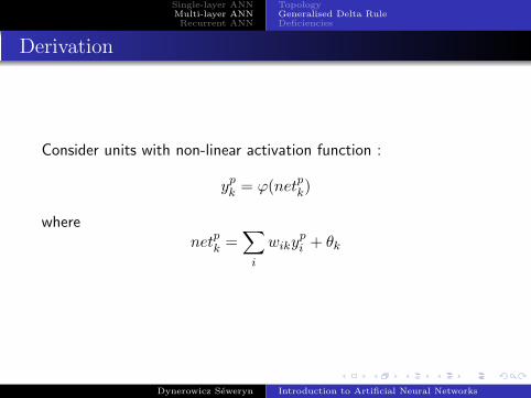
Derivation
Consider units with non-linear activation function :
ypk = ϕ(netpk)
wherenetpk =
∑i
wikypi + θk
Dynerowicz Seweryn Introduction to Artificial Neural Networks

Single-layer ANNMulti-layer ANNRecurrent ANN
TopologyGeneralised Delta RuleDeficiencies
Derivation (cont’d)
The modification we should apply to each weight is given by :
∆pwik = −γ∂Ep
∂wik
In which Ep, the total error is defined by :
Ep =12
No∑o=1
(dpo − yp
o)2
By using the chain rule we obtain :
∆pwik = −γ∂Ep
∂netpk
∂netpk∂wik
Dynerowicz Seweryn Introduction to Artificial Neural Networks

Single-layer ANNMulti-layer ANNRecurrent ANN
TopologyGeneralised Delta RuleDeficiencies
Derivation (cont’d)
The right derivative can be rewritten as :
∂netpk∂wik
= ypi
If we define
δpk = − ∂Ep
∂netpk
we obtain an update rule which is similar to the Delta Rule :
∆pwik = γδpky
pi
The problem now is to define this δpk for the different unit k in the
network.
Dynerowicz Seweryn Introduction to Artificial Neural Networks

Single-layer ANNMulti-layer ANNRecurrent ANN
TopologyGeneralised Delta RuleDeficiencies
Derivation (cont’d)
By using the chain rule, we rewrite δpk :
δpk = − ∂Ep
∂netpk= −∂Ep
∂ypk
∂ypk
∂netpk
The right derivative can be rewritten as :
∂ypk
∂netpk= ϕ′(netpk)
For the left derivative, we must consider two cases :
k is an output unit o ;
δpo = (dp
o − ypo)ϕ
′(netpo)
Dynerowicz Seweryn Introduction to Artificial Neural Networks
Single-layer ANNMulti-layer ANNRecurrent ANN
TopologyGeneralised Delta RuleDeficiencies
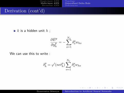
Derivation (cont’d)
k is a hidden unit h ;
∂Ep
∂yph
= −No∑o=1
δpowho
We can use this to write :
δph = ϕ′(netph)
No∑o=1
δpowho
Dynerowicz Seweryn Introduction to Artificial Neural Networks

Single-layer ANNMulti-layer ANNRecurrent ANN
TopologyGeneralised Delta RuleDeficiencies
Derivation (cont’d)
The two equations :
δpo = (dp
o − ypo)ϕ
′(netpo) (1)
δph = ϕ′(netph)
No∑o=1
δpowho (2)
Define a recursive procedure which can be used to adjust theweights of the network. It constitutes the Generalised Delta Rulefor a feed-forward network of non-linear units.
Dynerowicz Seweryn Introduction to Artificial Neural Networks

Single-layer ANNMulti-layer ANNRecurrent ANN
TopologyGeneralised Delta RuleDeficiencies
Learning rate and Momentum
In order to have fast convergence with a stable solution, amomentum term is added to the variation of the weight.
∆wjk(t + 1) = γδpky
pj + α∆wjk(t)
Instability of the solution is countered because the change in theweights is dependant of the previous change.It is possible to increase the learning rate γ without causingoscillation in the solution.
Dynerowicz Seweryn Introduction to Artificial Neural Networks

Single-layer ANNMulti-layer ANNRecurrent ANN
TopologyGeneralised Delta RuleDeficiencies
Learning rate and Momentum
a) γ → 0b) γ → 1c) γ → 1 with a momentum term added
Dynerowicz Seweryn Introduction to Artificial Neural Networks

Single-layer ANNMulti-layer ANNRecurrent ANN
TopologyGeneralised Delta RuleDeficiencies
Deficiencies
Network paralysis : as the network is trained, the weightscan increase to very high values (either positive or negative),so does netj . Because of the sigmoid function, the activationwill be very close to zero or very close to one. In that case,the back-propagation algorithm may come to a standstill.
Local Minima : because of the shape of the error functionfor a complex network, the gradient method can find itselftrapped in a local minima. Some methods (probabilistic) canavoid this problem but are very slow. It is also possible toincrease the number of hidden units without going beyond acertain threshold.
Dynerowicz Seweryn Introduction to Artificial Neural Networks

Single-layer ANNMulti-layer ANNRecurrent ANN
Jordan NetworkHopfield Network
3 Single-layer ANNPerceptronAdalineLimitations
4 Multi-layer ANNTopologyGeneralised Delta RuleDeficiencies
5 Recurrent ANNJordan NetworkHopfield Network
Dynerowicz Seweryn Introduction to Artificial Neural Networks

Single-layer ANNMulti-layer ANNRecurrent ANN
Jordan NetworkHopfield Network
Jordan Network
Proposed by Jordan in 1986.
Activation values of the output units are fed back into the inputlayer through so-called state units.
The weights from output units to these state units is fixed to +1.
Thus, the learning rules which apply to multi-layer ANN can beused to train Jordan Networks.
Dynerowicz Seweryn Introduction to Artificial Neural Networks

Single-layer ANNMulti-layer ANNRecurrent ANN
Jordan NetworkHopfield Network
Jordan Network
Dynerowicz Seweryn Introduction to Artificial Neural Networks

Single-layer ANNMulti-layer ANNRecurrent ANN
Jordan NetworkHopfield Network
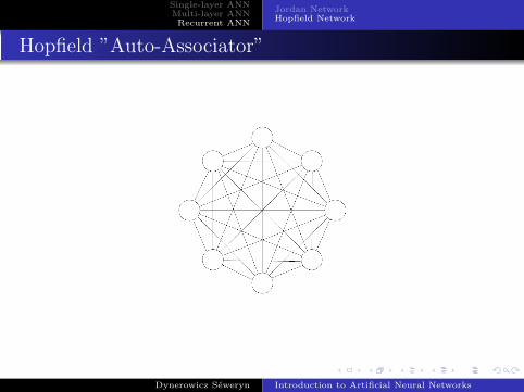
Hopfield Network
Proposed by J. Hopfield in 1982.
Consists of a fully-interconnected network of N neurons which areboth input and output.
Updates are made asynchronously and independently.
Activation values are binary (+1 / -1).
Can be used as an associative memory or for optimisation problems(salesman problem).
Dynerowicz Seweryn Introduction to Artificial Neural Networks
Single-layer ANNMulti-layer ANNRecurrent ANN
Jordan NetworkHopfield Network
Hopfield ”Auto-Associator”
Dynerowicz Seweryn Introduction to Artificial Neural Networks

ApplicationConclusion
Smart sweepers
6 ApplicationSmart sweepers
7 Conclusion
Dynerowicz Seweryn Introduction to Artificial Neural Networks

ApplicationConclusion
Smart sweepers
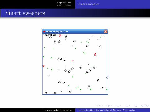
Smart sweepers
Objective : train minesweepers to pick up mines in a2-dimensionnal field.
Parameters of the network :
Topology : Feed-forward multi-layer ANN.
4 input units6 hidden units on one layer2 output units
Activation function : sigmoid function.
Learning rule : genetic algorithm.
Dynerowicz Seweryn Introduction to Artificial Neural Networks

ApplicationConclusion
Smart sweepers
Smart sweepers
Input is composed of two vectors :
Vector defining the direction of the closest mine.
Vector defining the direction towards which the minesweeperis pointing.
Output is composed of two components, the speeds of left andright track.
Dynerowicz Seweryn Introduction to Artificial Neural Networks

ApplicationConclusion
Smart sweepers
Smart sweepers
Each minesweeper has its own set of weights.
The ANN works for a certain amount of time T . During this periodof time, each mine found increases the fitness of the sweeper.
Afterwards, the GA starts running to create the new generation ofweight sets.
Dynerowicz Seweryn Introduction to Artificial Neural Networks
ApplicationConclusion
Smart sweepers
Smart sweepers
Dynerowicz Seweryn Introduction to Artificial Neural Networks

ApplicationConclusion
Smart sweepers
Smart sweepers
Dynerowicz Seweryn Introduction to Artificial Neural Networks

ApplicationConclusion
Conclusion
Single-layer ANN :
Limited representationnal power : restricted to linear classifier
Linearity of the system ⇒ convergence to the optimal solution(optimal weight vector)
Multi-layer ANN :
Unlimited representationnal power : can model non-linearproblems
Non-linearity doesn’t guarantee the convergence to an optimalsolution
Dynerowicz Seweryn Introduction to Artificial Neural Networks

ApplicationConclusion
Conclusion
Choice of a representative learning sample is essential toobtain the ”expected” behavior and to avoid over-fitting.
Combination with other approaches can prove to be effective(genetic algorithms for instance)
Dynerowicz Seweryn Introduction to Artificial Neural Networks

ApplicationConclusion
References
B. Krose, P. van der SmagtAn introduction to Neural Networks, Eighth edition.
S. SinghNeural Network Recognition of Hand-printed Characters.
Dynerowicz Seweryn Introduction to Artificial Neural Networks