STATA: An Introduction with Applied Econometric Applications Sean P. Corcoran University of Maryland November 20, 2002 NOTE: This handout is preliminary and incomplete.

Introduction: STATA Essentials About STATA STATA has become one of the most popular programs among researchers in applied microeconomics. STATA was written by labor economists, so naturally many of its procedures are designed with economic applications in mind. Unlike SAS, STATA has many common econometric procedures--such as two-stage least squares, fixed effects regression, and correction for sample selection--that can be executed with simple one-line commands.1 On the rare occasion that the built-in functions in STATA are insufficient, one can usually find someone in STATA's large user network who has already programmed the necessary code. These user-written commands (''.ADO'' files) can often be installed directly to STATA via the Internet, with only a few mouse clicks. In STATA, datasets are loaded and processed in RAM. The advantage of this design is speed--with little reliance on the hard disk, most STATA programs run very fast. The downside is that the size of your RAM will determine how large of a data set you can use. In most cases, this will not prove to be much of a constraint. However, some projects will simply be too big for STATA, and will require another package (such as SAS) that uses hard-disk based operations. This short handout is intended to introduce you to STATA and its many functions. You will learn how to read, create, and modify datasets, produce basic summary tables and graphs, and perform some basic analyses. I will assume that you are using Intercooled STATA 7 for Windows (although STATA is available on other platforms, like Mac and UNIX). Examples will be primarily microeconomic in nature; this is the case not only because my training is in applied micro, but because STATA is most widely used in the analysis of cross-sectional and panel data. What is most important is that you learn the general syntax of STATA commands--once you get the hang of it, you can easily incorporate additional commands into your repertoire via STATA's extensive help system, described in more detail in Section 1.2. STATA Help and References Two of STATA's most notable features are its well-designed help menus and its vast user network. Wisely, the STATA Corporation takes full advantage of the accumulated human capital of its users, and has incorporated user comments, web links, and programs directly into its help menus. These features, as well as some other useful references are briefly described below: 1For an economist's view of how statistics and econometrics packages compare on a number of dimensions, see MacKie-Mason's ''Econometric Software: A User's Review'' in the Journal of Economic Perspectives, 6:4 (1992), pp. 165-187.

1) STATA Help Menus: as in other software packages, STATA's help files can be queried by clicking on HELP, SEARCH from the menu bar. Unlike other packages, however, I find these menus extremely useful. In addition to syntax guidance, these menus include web links to frequently asked questions (e.g. ''what is seemingly unrelated regression?''), examples, and user programs. On many topics, you will even find references to relevant pages in Greene's Econometric Analysis.

2) STATA's Website: http://www.stata.com/. A terrific resource with technicial support, frequently asked questions, etc.

3) STATAList: a daily email digest with very knowledgeable contributors. You can subscribe to this digest via the STATA website.

4) STATANews and STATAJournal: a newsletter and reviewed journal published by STATA. See STATA's website for more info.

5) Other Useful Websites: http://statcomp.ats.ucla.edu/stata/. The UCLA STATA portal--a wealth of STATA resources, tutorials, and examples. Also see http://www.econ.ucdavis.edu/faculty/cameron/stata/stata.html for other useful tutorials and examples.

6) ''Statistics with STATA (updated for Version 7)'' by Lawrence C. Hamilton, Duxbury Press, 2001.

7) ''A Handbook of Statistical Analysis using STATA, 2nd edition'' by Sophia Rabe-Hesketh and Brian Everitt, CRC Press, 2000. Mostly for epidemiologists, but still a useful text.

The STATA Interface From the START menu, launch Intercooled STATA 7.0. When you open STATA, you will initially see four windows: • Command: in this window you can issue commands to STATA, run programs, or

perform procedures on the active dataset. • Results: this is the equivalent of the SAS log and output windows. STATA messages

and output are sent to this window upon the execution of commands or programs. • Variables: this window lists all variables currently loaded into memory. • Review: this window keeps a running history of all commands that have been issued

to STATA from the command window. One useful feature of this window is the ability to click on past commands, which returns the line to the command window for editing or re-execution.

Note that commands can be issued to STATA interactively (via the command window) or in batch format. To write a STATA program for batch processing, click on the button that looks like a white envelope--this activates the Do-File Editor, a text editor that can be used to write and submit programs. Executable STATA programs end with the ''.DO'' extension. Some Basic Commands and Syntax A typical STATA program will consist of both executable and nonexecutable statements. Nonexecutable statements are programming comments that begin with a star (*). Executable statements are used to provide basic operating instructions, to read or modify data, or to describe or analyze data. In this section, we briefly summarize some useful executable statements that you may wish to include in your STATA program. Again, STATA commands can be included in a DO file, or typed individually into the

command window. If you are writing a program, no more than one command can be typed per line (and each command can only take up one line)--unless you define a delimiter. Delimiter definition is the first command summarized in the table below (note, throughout this document, all commands are printed in bold). For more detailed information about any of these commands, SEARCH on them in STATA's help menu. Command Description # delimit ; tells STATA that the semicolon denotes the end of

a line (allows you to extend commands past one line in a program).

set memory 10m tells STATA to use 10 megabytes of RAM (you may want to set this higher)

memory displays info about memory usage cd pathname changes the current working directory pwd displays working directory dir or ls shows all files in the working directory log using filename, replace creates a log file which stores all STATA messages

and output. filename can be a simple one word name (if you are saving to the working directory), or a full file specification, such as c:\corcoran\reglog.log. The replace option tells STATA to overwrite any existing log file under thatname. An append option allows you to append an existing log file. The default extension for log files is .SMCL. Use an explicit extension like .LOG or .TXT if you prefer.

log close closes the current .LOG file cmdlog using filename creates a .TXT file containing a history of all

commands typing into the command window. display expression can be used as a simple calculator, e.g. display 82

will output 64. type prints an ASCII file, e.g. type reglog.log clear clears any existing data from memory set matsize # sets the maximum number of variables that can be

included in any estimation procedure (replace the # sign with a number); the default is 40, but you can increase this as high as 400 in Intercooled STATA (note fixed effects dummies in panel data models are not counted).

exit quits STATA. do filename entered into the command window, tells STATA to

execute the do-file filename. set more off turns off all --more-- pauses in the STATA output

window. search command searches the help menus on a particular command. update connects to STATA via the internet, and allows you

to install the latest official updates (including ADO files).

net allows you to update STATA via the internet with the latest ADO files, help files, or datasets.

type filename displays the ASCII file filename in the results window. You can use this command for a quick view of your LOG file.

Notice the syntax of these commands--most STATA commands begin with a verb (e.g. display, describe, summarize) with a direct object or adverb following (e.g. a filename or variable name). Many STATA commands have additional options that you can specify. These commands always follow a comma at the end of the command. Let's look at a STATA program that has already been started for you. Copy text from the following document into your Do-File Editor: http://www.wam.umd.edu/ spcorcor/stata1.txt. In later sections, we will add commands to this program. Once you have copied the text, save this do-file to your disk, and then click on the ''Do Current File'' button at the top of the Do-File Editor--this will execute your STATA program. Note the messages that appear in the results window.

Creating STATA Datasets Reading Data from Other Sources STATA can read data from a number of different formats. The command line you use to read your data into STATA will depend on the format that your data is in. The table below summarizes some commands required to read and describe datasets. Command Description use filename loads a STATA-format dataset into memory

(discussed in Section 2.2) insheet [varnames] using filename loads a formatted ASCII dataset created by a

spreadsheet (e.g. comma-separated-values CSV format)

infile [varnames] using filename loads an unformatted (e.g. space delimited) ASCII dataset

infix [varnames colpointers] using filename loads a fixed-column ASCII dataset input [varnames] [data] reads data that immediately follows this statement edit opens STATA's spreadsheet-like editor for direct

input of data count displays the number of observations in memory describe describes the contents of the dataset in memory

(equivalent to SAS PROC CONTENTS)

list prints the entire contents of the dataset (equivalent to SAS PROC PRINT)

codebook gives detailed information about the contents of a dataset

Let's try reading a .CSV file containing data on local per-pupil revenues in Maryland school districts in 1990. Add the following lines to your existing STATA program, and then click on the run button. Notice that the describe command is abbreviated with desc; this is possible with any STATA command by using the minimum number of unique starting letters in the command. insheet using http://www.wam.umd.edu/spcorcor/mdschools.csv; count; desc; list; If the program runs successfully, the mdschools dataset will be loaded from the given web address, and the observation count, data description, and full contents will be output to the results window. You will also see the names of the variables in this dataset appear in the variables window (STATA already knows the names of these variables because they were included in the CSV file). In the event that your CSV file does not contain variable names, you can specify the names after the insheet statement as follows: insheet id school city state enrollment etc using mdschools.csv; Clear the mdschools data from memory by typing clear in the command window (and hitting ENTER). Space-delimited data is read in the same manner, but using infile instead of insheet. Let's try reading a space-delimited file by typing the following command in the command window (the next two example datasets were borrowed from the UCLA STATA web portal, described in Section 1.2; you can preview it in Notepad, if you wish):

infile gender id race ses schtyp str10 prgtype read write math science socst using http://www.wam.umd.edu/spcorcor/hs0.raw; desc;

Notice in this case variable names are listed in the infile command, and that the 'strn' indicator is placed before the character variable prgtype (n is the length of this variable).

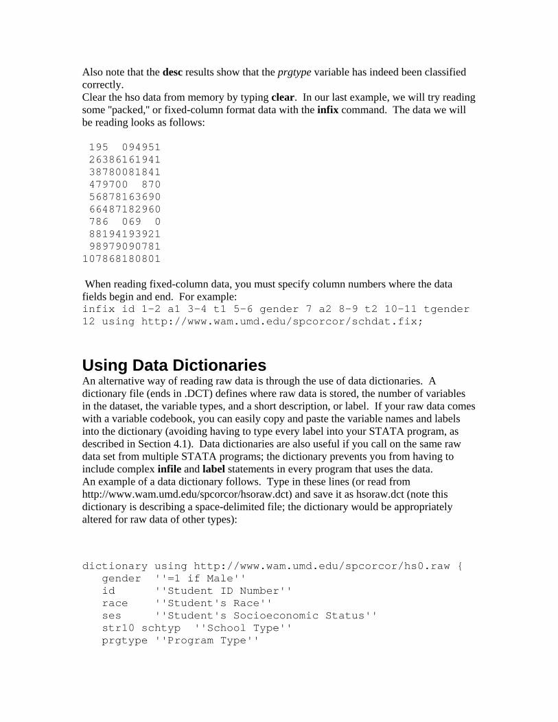
Also note that the desc results show that the prgtype variable has indeed been classified correctly. Clear the hso data from memory by typing clear. In our last example, we will try reading some ''packed,'' or fixed-column format data with the infix command. The data we will be reading looks as follows: 195 094951 26386161941 38780081841 479700 870 56878163690 66487182960 786 069 0 88194193921 98979090781 107868180801 When reading fixed-column data, you must specify column numbers where the data fields begin and end. For example: infix id 1-2 a1 3-4 t1 5-6 gender 7 a2 8-9 t2 10-11 tgender 12 using http://www.wam.umd.edu/spcorcor/schdat.fix;

Using Data Dictionaries An alternative way of reading raw data is through the use of data dictionaries. A dictionary file (ends in .DCT) defines where raw data is stored, the number of variables in the dataset, the variable types, and a short description, or label. If your raw data comes with a variable codebook, you can easily copy and paste the variable names and labels into the dictionary (avoiding having to type every label into your STATA program, as described in Section 4.1). Data dictionaries are also useful if you call on the same raw data set from multiple STATA programs; the dictionary prevents you from having to include complex infile and label statements in every program that uses the data. An example of a data dictionary follows. Type in these lines (or read from http://www.wam.umd.edu/spcorcor/hsoraw.dct) and save it as hsoraw.dct (note this dictionary is describing a space-delimited file; the dictionary would be appropriately altered for raw data of other types):

dictionary using http://www.wam.umd.edu/spcorcor/hs0.raw { gender ''=1 if Male'' id ''Student ID Number'' race ''Student's Race'' ses ''Student's Socioeconomic Status'' str10 schtyp ''School Type'' prgtype ''Program Type''

read ''Reading Score'' write ''Writing Score'' math ''Math Score'' science ''Science Score'' socst ''Social Studies Score'' };

This dictionary defines the file hso.raw as the source of the raw data, and provides labels for each variable in the dataset. Note that all variable names must be 8 characters or less; variable names must begin with a letter or underscore ; and numbers can be used in all but the first position of the variable name. Your STATA program (DO-file) can then call on the dictionary with one line--the infile command: infile using a:\hsoraw; (you do not need to include the .DCT extension in the infile command). Saving and Reading STATA Datasets Command Description use filename loads a STATA-format dataset into memory save filename saves a STATA-format dataset to the given

filename compress reduces the size of the dataset by storing the data in

the most efficient format Once your data is read into memory, you will likely want to save your data in STATA format. Before doing this, you can compress the data--this command tells STATA to save the data in the most efficient way possible. Re-open and compress the mdschools dataset by typing the following commands into the command window (or, adding to your program). The save command will save the mdschools dataset in STATA format (with the .DTA extension): insheet using http://www.wam.umd.edu/spcorcor/mdschools.csv; compress; save mdschools, replace; This command saves the new STATA dataset to the working directory; the replace option tells STATA to overwrite an existing version of the dataset. If you like, you can save STATA datasets directly to a filepath by typing the entire pathname in the save command. For example:

save c:\corcoran\dissertation\mdschools, replace; Clear the mdschools dataset from memory by entering clear into the command window. Now, try opening the new mdschools STATA dataset with the use command as follows. use mdschools;

Converting SAS and SPSS Data to STATA You can easily convert data from other formats--like SAS, SPSS, Matlab, Limdep, Excel, Lotus 1-2-3, and Access--to STATA format using STAT Transfer, a program available in the Econ grad lab (under Top Applications...Statistics). Just follow the simple prompts. STATA datasets can be exported as a CSV file (among other formats) using the outsheet command: outsheet name ncesid lrevp using md2.csv, comma; This exports the listed variables to a CSV file--the comma option indicates that we want a comma separated values file (tab delimited is the default).

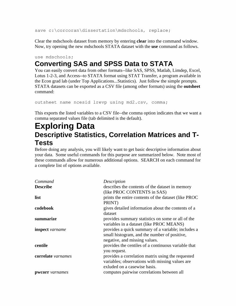
Exploring Data Descriptive Statistics, Correlation Matrices and T-Tests Before doing any analysis, you will likely want to get basic descriptive information about your data. Some useful commands for this purpose are summarized below. Note most of these commands allow for numerous additional options. SEARCH on each command for a complete list of options available. Command Description Describe describes the contents of the dataset in memory

(like PROC CONTENTS in SAS) list prints the entire contents of the dataset (like PROC

PRINT) codebook gives detailed information about the contents of a

dataset summarize provides summary statistics on some or all of the

variables in a dataset (like PROC MEANS) inspect varname provides a quick summary of a variable; includes a

small histogram, and the number of positive, negative, and missing values.

centile provides the centiles of a continuous variable that you request.

correlate varnames provides a correlation matrix using the requested variables; observations with missing values are exluded on a casewise basis.

pwcorr varnames computes pairwise correlations between all

specified variables; missing values affect deletion on a pairwise basis.

order orders the variables in the Variables window list as you select

aorder alphebetizes the variables in the Variables window list

ttest performs a simple t-test Let's use these commands to get an overview of a new dataset, NLS80, which has already been saved in STATA format. NLS80 contains informaiton on 935 men aged 28-38 who in 1980 were a part of the National Longitudinal Survey of Young Men (a dataset frequently used by labor economists; the variables are described in Appendix 1). Create a new program in the do-file editor called nls80.do, and add the following commands: # delimit ; cd a:\; log using nlslog, replace use http://www.wam.umd.edu/spcorcor/nls80; save nls80; desc; list; codebook; Note how the output for the desc, codebook, and list commands differ. Each provides varying degrees of descriptive information about all the variables in the dataset. You can view information about specific variables in the dataset by specifying variable names after the command. For example: codebook wage age; inspect wage; The inspect command is a useful command that gives you a rough histogram for a variable, along with counts of the positive, negative, and missing values. When listing multiple variable names, it is not always necessary to type the entire list. For example, one can use:

list exper-tenure;

(note the hyphen) to list all variables from exper to tenure (be sure to note the variable order in your variable window). If you wish, you can order variables in your Variables window any way you like, with the order command:

order educ age exper wage;

This command displays the education, age, experience, and wage variables first in your window. Using aorder alphebetizes your variables. You can generate summary statistics about some or all of the variables in memory with the summarize command. Try:

summarize; sum wage, detail;

(note the use of the abbreviation, sum). The detail option tells STATA to provide more than the default (mean, standard deviation, n, max, min) statistics. Another useful command is centile which provides specified centiles of the variable of interest. For example, the following command:

centile wage, centile(20,40,60,80,100);

displays the quintiles of the sample wage distribution. Correlation matrices can be generated with the command correlate (or corr) and pwcorr. For example, try:

corr wage educ exper; pwcorr wage educ exper age;

With pwcorr, you can add options that--for example--display the numbers of observations used, and the significance levels of each correlation coefficient: pwcorr wage educ exper age, obs sig; Finally, the ttest command can be used to perform simple hypothesis tests on means and differences in means. In the following example, the first command tests the hypothesis that the mean of the age variable is 33. The second tests the null hypothesis that there is no difference in the mean wage of black and nonblack men (the third adds options telling STATA to assume unequal variances, and test the hypothesis at the 90% significance level). The last command tests the hypothesis that the mean of the variable v1 differs from that of v2. Note, at any time you can set the default significance level with the command set level # (where # is a number like 90 or 95). ttest age = 33; ttest wage, by(black); ttest wage, by(black) unequal level(90); ttest v1 = v2;

Sorting Data and Using Conditions Command Description sort varname sorts the data in ascending order by the variable

varname gsort [+/-] varname sorts the data in ascending (+) or descending (-)

order by the variable varname if used in a command, conditions the action on some

clause in used in a command, applies the action only to a

subset of observations by varname: used preceding a command, requests that the action

be repeated by ''BY'' groups

Sorting in STATA is easy with the gsort and sort commands. Let's sort our NLS80 data in descending order by the wage variable (note sort only works in ascending order): gsort -wage; The IN condition allows you to take an action on a defined subset of observations. For example, now that our data is sorted in descending order, we might be interested in seeing a list of the top 10 largest wage earners. Add the IN condition as follows: list wage educ exper in 1/10;

The 1/10 tells STATA to list the variables wage, educ, and exper for the first ten observations (in our case, the ten largest). The IF condition is another easy way to condition your STATA commands. For example:

summarize wage if wage>3000; sum wage if educ==12; Logical operators are as follows: >, <, >=, <=, == and =. Note the double equals sign for equality conditions. When testing whether or not a variable is equal to one of a large list of possible values, use the inlist() function--e.g. sum wage if inlist(educ,12,13,14,15) will summarize the wage variable for those observations whose education level is equal to 12, 13, 14, or 15. Multiple conditions can be implemented, using AND (&), OR (), and NOT()--note, STATA only accepts the symbols--not the words AND, OR, and NOT. An example

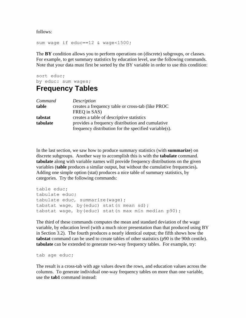
follows: sum wage if educ==12 & wage<1500; The BY condition allows you to perform operations on (discrete) subgroups, or classes. For example, to get summary statistics by education level, use the following commands. Note that your data must first be sorted by the BY variable in order to use this condition: sort educ; by educ: sum wages;

Frequency Tables Command Description table creates a frequency table or cross-tab (like PROC

FREQ in SAS) tabstat creates a table of descriptive statistics tabulate provides a frequency distribution and cumulative

frequency distribution for the specified variable(s).

In the last section, we saw how to produce summary statistics (with summarize) on discrete subgroups. Another way to accomplish this is with the tabulate command. tabulate along with variable names will provide frequency distributions on the given variables (table produces a similar output, but without the cumulative frequencies). Adding one simple option (stat) produces a nice table of summary statistics, by categories. Try the following commands: table educ; tabulate educ; tabulate educ, summarize(wage); tabstat wage, by(educ) stat(n mean sd); tabstat wage, by(educ) stat(n max min median p90); The third of these commands computes the mean and standard deviation of the wage variable, by education level (with a much nicer presentation than that produced using BY in Section 3.2). The fourth produces a nearly identical output; the fifth shows how the tabstat command can be used to create tables of other statistics (p90 is the 90th centile). tabulate can be extended to generate two-way frequency tables. For example, try: tab age educ; The result is a cross-tab with age values down the rows, and education values across the columns. To generate individual one-way frequency tables on more than one variable, use the tab1 command instead:

tab1 age educ;

Generating Simple Graphs Command Description hist generates a histogram of a categorical variable. graph generates a histogram-like density plot for a

continuous variable. When two variable names are specified, the default graph is a two-way scatterplot.

kdensity generates a smoothed kernal density plot of a continuous variable.

The table above lists some of the most common simple graph commands in STATA. Each is fairly self-explanatory--you will best understand what each command does by simply trying them and viewing the results (IQ and KWW are scores from the IQ and Knowledge of the World of Work tests, respectively): hist educ; hist age; graph wage; graph wage, normal; graph wage educ, twoway; kdensity iq; kdensity kww; graph iq kww; graph iq kww, jitter(2); graph wage educ exper, matrix; The normal option in the graph command fits a normal density curve to the density plot, while the jitter(2) option spreads identical observations in the scatterplot. The matrix option will produce a matrix of scatterplots. Graphs can be very easily copied and pasted into other documents--when the graph you want to copy is displayed, select Edit...Copy Graph, and paste directly into your word processor. Using Weights For some applications, you may wish to use sample weights in generating sample statistics, correlation matrices, or regressions. This is typically accomplished by including weighting instructions in your STATA command. STATA uses four different types of weights: 1) fweights: or frequency weights; these weights indicate the number of duplicated

observations. 2) pweights: or sampling probability weights; these represent the inverse of the

probability that the observation was sampled. 3) aweights: or analytic weights; these weights are inversely proportional to the variance

of the observaton. For example, if the observations are sample averages, one would want to use the N's (sample size that generated the individual averages) as the aweight.

4) iweights: or importance weights; the definition of iweights varies depending on the application.

Suppose you have a weighting variable called w1. The syntax for generating (weighted) sample statistics for the variable wage would be as follows (use brackets to enclose the weight instruction, as shown): summarize wage [aweight=w1]; aweights give more weight to observations with high w1, and less weight to observations with low w1 (i.e. the observations with high w1 are assumed to have lower variance and are thus weighted more heavily)--for most applications, this is probably the appropriate weight type (it is also the default for many commands, including summarize; to use the default weight just use [weight=w1]).

Modifying Data Labeling and Renaming Variables You will likely want to add descriptive labels to your dataset. The following table summarizes some commands frequently used to label or rename variables (or datasets) in STATA: Command Description label data ''text'' applies a label to the dataset label variable varname ''text'' applies a label to the named variable notes varname: ''text'' applies user notes to the named variable label define defines a coding for a categorical variable (like

PROC FORMAT in SAS) label values applies the defined coding to a specific variable rename renames a variable Let's add a label that describes the contents of the NLS80 dataset with the label data command; as well as variable labels that describe the individual variables with the label variable command (abbreviated label var). The notes command adds user notes to the IQ variable (just type notes alone to view the user notes). label data ''National Longitudinal Survey of Young Men, Aged 28-38 in 1980, 935 cases''; label var wage ''Monthly earnings''; label var hours ''Average weekly hours''; label var iq ''IQ Score''; label var kww ''Knowledge of World of Work Score''; label var educ ''Years of Education'';

label var exper ''Years of Work Experience''; label var tenure ''Years with Current Employer''; label var age ''Age, in Years''; label var married ''=1 if Married''; label var black ''=1 if Black''; label var south ''=1 if lives in South''; label var urban ''=1 if lives in SMSA''; label var sibs ''Number of Siblings''; label var brthord ''Birth Order''; label var meduc ''Mothers Years of Education''; label var feduc ''Fathers Years of Education''; notes iq: ''IQ ranges from 50-145''; Renaming variables is simple with the rename command: rename black blk; You can use the desc command to view all of these changes and additions (note that the label for black is not lost when the variable is renamed). Finally, you can add a text coding to numeric categorical variables with the label define and label values commands. Label define will define a coding that can be applied to any variable using the label values command: label define urb 1 lives in MSA 0 lives outside MSA; label values urban urb;

Keeping and Dropping Variables and Observations The keep and drop commands can be used to eliminate variables or observations. keep or drop plus variable names will tell STATA to keep or drop the listed variables (your decision to use keep instead of drop will depend on whether the number of variables you intend to keep is smaller than the number that would be dropped). keep or drop together with an IN or IF condition will tell STATA to keep or drop certain observations. For example (don't try these with the NLS data without saving first): keep in 1/20; will keep observations 1 - 20; and drop if wage==.; drop if missing(wage); are equivalent statements that drop all observations where the wage is missing (as in SAS, the period can represent missing values). The missing function returns a 1 or ''true'' for those observations where the wage variable is missing. Creating New Variables

Command Description generate creates a new variable replace replaces one value with another value egen ''extended generate''--uses special functions in

creating new variables encode changes a string variable to numeric recode reassigns new values to a discrete or continuous

variable xi creates dummy variables based on the values of a

specified variable The standard command in STATA for creating a new variable is generate (or gen), with the general syntax: gen newname = expression. The following commands add (and label) some new variables to our NLS80 data: gen wkwage=(wage/4); gen lwkwage=ln(wkwage); gen exper2=exper2; gen age2=age2; gen hipared=max(feduc,meduc); label var wkwage ''Weekly Wage'' label var lwkwage ''Log of Weekly Wage''; label var exper2 ''Experience Squared'' label var age2 ''Age squared''; label var hipared ''Highest Education of Parents''; The following table is a sample of some of the mathematical and statistical functions you may wish to use in your gen commands (note there are dozens of mathematical, statistical, time series, date, string, and special STATA functions; search on functions for a complete list):: abs(x) returns the absolute value of x sqrt(x) returns the square roexp(x) returns the exponential of x normden(z) returns the standandln(x) returns the log of x norm(z) returns the cumulatilog10(x) returns the log (base 10) of x chi2(df,x) returns the cumulati

degrees of freedom)max(x1,x2,..) returns the maximum of the listed variable values ttail(df,t) returns the probabili

with df degrees of frmin(x1,x2,..) returns the minimum of the listed variable values uniform() reutrns a random nu

distribution To change a variable's value once it has been created, you must use the replace (or

recode) commands. For example, suppose you wished to rescale the wage2 variable (a copy of wage) to thousands of dollars: gen wage2=wage; replace wage2=wage2/1000; Unlike SAS, a command in STATA such as gen wage=wage/1000 would not work in STATA. The replace command must be used as above. The recode command is similar to replace in that it replaces values as you specify. In the following example, the new variable wageqtle denotes the (approximate) quintiles that the observations' wage is in: gen wageqtle=wage; recode wageqtle 0/616=1 616/808=2 808/1000=3 1000/1250=4 1250/4000=5; recode is also useful when one wants to recode missing values from, say, 99 to a period. For example, you could use: recode somevar 99=.; The creation of dummy variables can be accomplished a number of different ways. In the simplest case, you may want to create a variable that equals one if a condition holds, and equals zero otherwise. For example, to create a dummy variable in the NLS data that equals one when the individual is a high school graduate, you can use either of the following methods: gen hsgrad=(educ>=12); gen hsgrad=0; replace hsgrad=1 if educ>=12; In other situations you may wish to create dummies for a large number of possible values of a variable (e.g. state dummies) or a large number of possible combinations of variable values (e.g. state x year dummies). The following is an example of both possibilities (note, there are methods for defining dummy variables directly in a regression statement; this will be discussed in Section x.x.): xi i.educ; *defines dummies for each level of educ; tabulate educ, gen(eddum); *does same thing; drop I*; *drops the dummies created in the xi statement (which start with ); xi i.educ * i.age; The second xi command will create dummies for both the educ and age variable, as well

as all possible educ x age interactions. The egen command is an extremely versatile command in STATA for creating new variables. egen can, for example, create a new variable that contains the overall or within-group mean of another variable. The following example creates two new variables--avgwage and avgwageg that contain the overall and within-education group mean wages: egen avgwage=mean(wage); egen avgwageg=mean(wage), by(educ); gen wagedif=wage - avgwage; Some of the other functions that can be used with egen are listed below (there are literally dozens of these--search on egen for the complete list): diff(x1,x2) returns a dummy equal to one when the value of

variable x1 equals that of x2, and zero otherwise ma(exp),t(#) returns a #-period moving average of variable exp max(x1) returns the max of variable x1 min(x1) returns the min of variable x1 mean(x1) returns the mean of variable x1 median(x1) returns the median of variable x1 mtr(year,income) returns the marginal tax rate for a married couple in

the US with income level income in year year pc(exp) returns the observation's percent of the total, based

on the variable exp rank(exp) returns the rank of the observation, based on the

variable exp sd(exp) returns the standard deviation of the variable exp std(exp) returns the standardized (mean 0, standard

deviation 1) value of exp Merging Datasets text here

OLS Regression A Basic Regression In this section we will use the regress and related commands to run a basic human capital earnings regression. The following table summarizes some important commands related to OLS regression: Command Description regress performs traditional OLS regression regress, robust performs OLS, computing robust standard errors

regress, cluster() performs OLS, with clustered standard errors local a STATA macro command you can use to create a

regressor shortcut list vce post-estimation, displays the variance-covariance

matrix of the coefficient estimates predict post-estimation, creates new varaibles containing

predicted values, residuals, or other values test post-estimation, performs a Wald test of linear

restrictions Let's estimate a regression where log weekly wage is the dependent variable, and education, experience, and experience squared are independent variables using the regress (reg) command. STATA automatically adds a constant to every model unless otherwise specified: reg lnwkwage educ exper exper2; reg lnwkwage educ exper exper2, robust; The robust option tells STATA to report robust (Huber-White-Sandwich) standard errors (i.e. the variance covariance matrix of beta-hat in the presence of heteroskedasticity, or X X 1 G X X 1 , where the G matrix is a diagonal matrix of squared estimated

residuals). Adding a cluster(varname) option will cluster standard errors, based on the variable varname. Note, you can use IN, IF, and BY conditions with regression, as well as weights (see section 2.5). Dummy variables can be requested directly in the reg command, by preceding reg with xi: and including an i. before the variables that serve as the source of the dummies. For example, including i.educ (as in the example below) will tell STATA to include dummy variables for every possible level of educational attainment (one level is automatically omitted). Interaction effect dummies can be included exactly as described in Section 3.3. The drop statement drops all of the dummies created in reg. xi: reg lnwage exper exper2 i.educ; drop I*; To avoid typing the same list of regressors over and over again, you can use the local command (a STATA local macro command) to define a shortcut list of regressors. For example, the following command defines xlist to be the vector of variables (educ, exper, exper2), and then uses xlist in the reg command. local xlist educ exper exper2; reg lnwkwage `xlist'; *note a rightward sloping single quote precedes xlist; Typing the vce command alone will output the variance-covariance matrix of the coefficient estimates to the results window (and log). You can perform a Wald (F) test of

linear restrictions using the test command, as the following examples show: test exper2; test exper=exper2; test educ=.02; test is one of STATA's post-estimation commands (search on postest for a complete list of these) that can be performed after any estimation command (such as reg, logit, etc). The first example above tests the hypothesis that the exper2 coefficient is equal to zero, the second tests the hypothesis that the exper coefficient is equal to the exper2 coefficient, and so on. Search on the commands lrtest and testnl for instructions on how to perform likelihood ratio tests and Wald tests of nonlinear restrictions. Another post-estimation command is predict, which allows you to create new variables in your dataset that contain the fitted values (y-hats), residuals (u-hats), confidence interval limits, and so on. The following example creates two new variables--yhat and uhat--that contain fitted values (specified with the xb option) and estimated residuals (specified with the resid option): predict yhat, xb; predict uhat, resid;

Regression Diagnostics The following table summarizes some useful commands to use after the regress command. Command Description kdensity varname, normal produces normal density plot of varname (can use

with residuals uhat to check for normality rvfplot plots residuals vs. fitted values rvpplot varname plots residuals vs. values of some regressor

(varname) pnorm varname produces normal probability plot of varname (can

use with residuals uhat) whitetst performs White's general test for

heteroskedasticity. An ADO file that must be installed.

bpagan varname performs Breusch-Pagan Lagrange Multiplier test for heteroskedasticity, conditional on a set of variables assumed to influence the error variance (varlist). An ADO file that must be installed.

dwstat computes the Durbin-Watson d statistic Most of the above commands are self-explanatory. For example, once you have created the estimated residual variable uhat in the last section, you can plot a kernal density function as follows:

kdensity uhat, normal; The whitetst and bpagan commands are the first user-programmed (.ADO) commands that we have encountered in this handout. It is probable that these commands have not yet been installed in your version of STATA, however adding them to your available list of STATA commands is quite simple. For example, search on the word bpagan in your STATA help menu. You should see the topic Tests for Heteroskedasticity in Regression Error Distribution, and a topic number (sg137). To install the ADO files, click on the topic number sg137 and you will see an hyperlink that will install the file directly to your version of STATA (assuming you have an internet connection)--it's as simple as that. Once the file has installed (this takes only a few seconds), you can search again on bpagan; you will now be able to view the bpagan help screen, which contains syntax information, and the like. Follow similar steps to install the whitetst ADO file. Formatting Regression Output The user-programmed outreg command will quickly become your favorite STATA command. outreg sends your regression output directly to a tab-delimited file, with your output in a standard format often found in journal articles (with standard errors in parentheses, stars denoting statistically significant coefficient estimates, and so on). If it has not already been installed, install outreg following the steps outlined in Section 4.2 for installing ADO files. Once outreg is installed, it can follow any estimation command, such as regression, logit, probit, etc. For example, if we wanted to output our human capital regression results from section 4.1 to the tab-delimited file results.out (in the current working directory), we would do the following: reg lnwkwage educ exper exper2; outreg using results.out, se bdec(5) replace; The result will be a table with regressors listed down the rows, and estimated coefficients and standard errors in parentheses reported in a column titled (1). You can import this tab-delimited fiile into Microsoft Excel (or a Word table)--however, for best results, choose ''text'' as the desired format for every column in Excel, when prompted (otherwise standard errors in parentheses are read as negative numbers). The se option tells outreg to output the coefficient standard errors (the default is t-statistics), while bdec(5) requests that coefficient estimates be reported to five decimal places. As in other commands, replace tells STATA to replace any existing file by the name of results.out. Some other useful options are tdec(#) (the number of decimal places for reported t-statistics), noparen (requests no parentheses around standard errors), nocons (requests that no constant be reported), and noaster (requests no asterisks next to statistically significant results). In the next example, we add two additional regressors to the regression specification. The second outreg command (with the append option) will add these results to the existing results.out file (under a column titled (2)), with all coefficients properly matched up by rows:

reg lnwkwage educ exper exper2 tenure married; outreg using results.out, se bdec(5) replace append;

Instrumental Variables and 2SLS Estimating a linear regression using instrumental variables (or two-staged least squares) is straightforward with the ivreg command. For example, suppose you wish to add the IQ variable to your regression specification as a proxy for unobserved ability, but wish to instrument for IQ using the KWW score, mother's education, and father's education. In this case, use ivreg as follows: ivreg lnwkwage educ exper exper2 (iq=kww meduc feduc), robust; The terms in parentheses indicate that IQ is one of the regressors, and that kww, meduc, and feduc are the first-stage instruments for IQ. Like all other STATA estimation commands, ivreg has a number of additional options (including robust, as in reg), and can include IF, IN, and BY conditions, weights, an outreg command, and so on. Including the option first after the comma will display the first-stage results. To perform a Hausman specification test (on all the estimated coefficients) using the IV and OLS results, you can use the hausman command as follows: ivreg lnwkwage educ exper exper2 (iq=kww meduc feduc); hausman, save; regress lnwkwage educ exper exper2 iq; hausman, constant sigmamore; The order of these commands is important--first you estimate the less efficient (but consistent) model (IV), you save the results to memory, then you estimate the more efficient model (OLS), and run the hausman command again. The resulting output will be IV and OLS coefficient estimates presented side-by-side, along with the Hausman test statistic (where under the null hypothesis IV is unnecessary; if this hypothesis is rejected, OLS estimates are inconsistent and therefore IV is appropriate). [Note: at the moment, I'm not sure how to perform a Hausman test on the IQ coefficient alone. I do know that you can manually obtain the coefficients and standard errors of the coefficients using matrix commands as below--please let me know if you know of a better way to do this]. ivreg educ exper exper2 (iq=kww meduc feduc); matrix iv1=e(b); *saves the coefficient estimates from the IV regression; matrix iv2=e(V); *save the VCOV matrix from the IV regression; regress educ exper exper2 iq; matrix ols1=e(b); matrix ols2=e(V); * use matrix operations to obtain individual coefficients and standard errors for Hausman

test; Probit and Logit Models The following commands are used in estimating qualitative dependent variable models in STATA: Command Description probit estimates maximum likelihood probit model dprobit estimates maximum likelihood probit model,

reports marginal effects instead of coefficients mfx computes marginal effects or elasticities based on

most recent estimation logit estimates maximum likelihood logit model logistic estimates maximum likelihood logit model, reports

odds ratios instead of coefficients mlogit estimates maximum likelihood mulinomial

(polytomous) logistic regression oprobit estimates ordered maximum likelihood probit

model Traditional probit models are estimated by maximum likelihood, using one of two STATA commands--probit or dprobit. The only difference between the two is what estimates are reported (coefficient estimates in probit and marginal effects in dprobit). Let's try estimating a probit model using each (for sake of example, ignore the obvious econometric problmes associated with this model): dprobit married iq wage age urban south black; probit; * note second command assumes same model variables; The dprobit command reports the marginal effect on the probability that Y=1 from an infintesimal change in each continuous variable, and the discrete change in the probability for dummy variables. If you specify the classic option with dprobit, you will get the marginal effects calculated at the mean values of all regressors (including dummies). The post-estimation command mfx allows more flexibility in specifying the exact values of x you wish you calculate your marginal effects. For example, after the probit command, you can issue the following command: mfx compute, at(south=0, black=1, urban=0); which tells STATA to compute the estimated marginal effects for a black male who does not live in the south, or in an urban area. Notice the standard errors of the marginal effects are also displayed. If you do not specify values in the at( ) option, the default is to compute marginal effects using the default method of the probit command. Other values

such as median and zero can be included in the at( ) option. The mfx command can also calculate elasticities with the coefficient estimates. The options eyex, dyex, and eydx all represent elasticities that can be computed (note eydx represents, for example, the percentage change in y resulting from a unit change in x): mfx compute, eydx at(mean black=0); Logit models are estimated using exactly the same syntax as probit above (there is no dlogit equivalent of dprobit). Panel Data: Fixed and Random Effects text here Heckman Correction for Sample Selection