Embed Size (px)
Citation preview

HP Prime Workshop Materials Version 1.3
© 2013 by HP Calculators Page 1 of 32
Introduction
HP Prime is the latest advanced graphing calculator from Hewlett-Packard. It incorporates a full-
color, multi-touch screen and comes pre-loaded with 18 HP Apps. HP Prime has a Home view,
with a history of your numerical calculations, as well as a CAS view, with a history of your
symbolic computations.
HP Prime has three design principles:
Provide a high degree of mathematical fidelity across multiple mathematical representations
Give students the touch-active experiences with mathematics that they have come to expect
from display technologies
Deliver a simple and seamless experience for mathematical exploration and problem-solving
Home and CAS
With HP Prime, you can choose whether to operate numerically in the Home view or
symbolically using the CAS in the CAS view. For example, press H and enter 8 in the
Home view to see 2.828… or press K and enter the same expression in the CAS view to see
22 .
Things you can do in both CAS and Home views:
Tap an item to select it or tap twice to copy it to the command line editor
Tap and drag up or down to scroll through the history of calculations
Press Z to retrieve a previous entry or result from the other view
Press the Toolbox key (D) to see the Math and CAS menus as well as the Catalog
Press F to open a menu of easy-to-use templates
Press J to exit these menus without making a selection
Tap , , and menu buttons once to activate
RPN Note: HP Prime supports RPN entry. In Home Settings (S H), navigate to Entry and
select RPN. These workshop materials use the default Textbook setting.
Calculation History • Tap to select an entry
• Tap twice to copy it to
the command line
Command Line Editor • 2D textbook format
Menu Buttons
• Tap to activate • Context-Sensitive
CAS View Home View
HP Prime Workshop Materials Version 1.3
© 2013 by HP Calculators Page 2 of 32
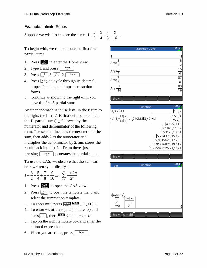
Example: Infinite Series
Suppose we wish to explore the series ...16
9
8
7
4
5
2
31
To begin with, we can compute the first few
partial sums.
1. Press H to enter the Home view.
2. Type 1 and press E
3. Press + 3 n 2 E
4. Press c to cycle through its decimal,
proper fraction, and improper fraction
forms
5. Continue as shown to the right until you
have the first 5 partial sums
Another approach is to use lists. In the figure to
the right, the List L1 is first defined to contain
the 1st partial sum (1), followed by the
numerator and denominator of the following
term. The second line adds the next term to the
sum, then adds 2 to the numerator and
multiplies the denominator by 2, and stores the
result back into list L1. From there, just
pressing E generates the partial sums.
To use the CAS, we observe that the sum can
be rewritten symbolically as
0 2
21...
16
9
8
7
4
5
2
31
nn
n
1. Press K to open the CAS view.
2. Press F to open the template menu and
select the summation template
3. To enter n=0, press ASR> 0
4. To enter +∞ at the top, tap on the top and
press+, then S 9 and tap on ∞
5. Tap on the right template box and enter the
rational expression.
6. When you are done, press E

HP Prime Workshop Materials Version 1.3
© 2013 by HP Calculators Page 3 of 32
HP Apps
HP Apps are designed to explore mathematical topics or solve problems. All HP Apps have a
similar structure, with numeric, graphic and symbolic views to make them easy to learn and easy
to use. Fill the app with data while you work, and save it with a name you’ll remember. Then
reset the app and use it for something else. You can come back to your saved app anytime-even
send it to your colleagues! HP Apps have app functions as well as app variables; you can use
them while in the app, or from the CAS view, Home view, or in programs.
Press I to see the App Library. Drag with your finger to browse the library, then tap the icon
of the app you want to use. The HP Apps are color-coded for easy identification:
5 graphing apps (blue) to explore graphs –including the new Advanced Graphing App!
2 Special apps (red): the Geometry app and the Spreadsheet app
4 Statistics Apps (purple) for descriptive and inferential statistics and data collection
4 Solver Apps (orange) for solving specific types of problems (triangles, finance, etc.)
3 Explorer Apps (green) for investigating a function’s equation and its graph
HP Apps
App Functions
App Variables
App Views

HP Prime Workshop Materials Version 1.3
© 2013 by HP Calculators Page 4 of 32
The Function App
The Function App gives you all the tools you need to explore the properties of functions,
including plotting their graphs, creating tables of values, and finding roots, critical points, etc.
1. Press I and tap on the Function icon.
The app opens in Symbolic view.
2. Enter 6
82X
in F1(X)
3. Enter 12
X in F2(X)
4. For each function, tap on the color picker to
choose a color and check/uncheck it to
select/deselect it for graphing
5. Press P to see the graphs of your
checked functions
In Plot view, tap to open the menu. The
menu buttons are:
Zoom: opens the Zoom menu
Trace: toggles tracing off and on
Go To: enter a specific x-value and the
tracer will jump to it
Fcn: opens a menu of analytic functions
Defn: displays the definition of a function
Menu: opens and closes the menu
Things you can do:
Press < or > to see that you are currently
tracing on F1(X)
Tap anywhere on the display and the tracer
will jump to the x-value indicated by your
finger tap while still remaining on the
function being traced.
Press \ or = to jump from function to
function for tracing
Tap and drag to scroll the graphing window
Press + and w to zoom in and out on
the cursor

HP Prime Workshop Materials Version 1.3
© 2013 by HP Calculators Page 5 of 32
The Fcn Menu
In the following examples, we will use the options in the Fcn menu to explore our two functions.
Roots
First, we will find one of the roots of our
quadratic function, F1(X).
1. Tap anywhere near the left-most root of
the quadratic (around x=-7)
2. Tap to open the menu (if
necessary)
3. Tap to open the Fcn menu
4. From the list, select Root, either by
tapping on it, using the direction keys, or
pressing x.
5. The value of the root (x=-6.928…) is
displayed
6. Press to show the exact location
of the cursor and to exit
Intersection
We will now find the left-most point of
intersection of the two graphs.
1. With the cursor still at the root from the
previous example, tap to open the
Fcn menu and select Intersection
2. A pop-up menu gives you the choice of
finding the intersection with F2(X) or
the x-axis. Press to select F2(X).
3. The intersection is displayed as shown to
that right
Slope
The Slope option in the Fcn menu works
similarly to Root, except that the slope
continues to be displayed as you trace the
function, until is pressed.

HP Prime Workshop Materials Version 1.3
© 2013 by HP Calculators Page 6 of 32
Signed Area
Suppose you wish to find the signed area
between the curves, from x=-9 to x=10.
1. Tap to open the Functions menu
and select Signed Area…
2. Tap near x=-9, use the direction keys to
move the cursor to x=-9 exactly, and tap
.
3. Now tap near x=10 and use the direction
keys to move the cursor to x=10 exactly
With the touch display, navigation is
improved and the experience is more
interactive.
As you move the cursor, the area between
the curves is filled in graphically. The color
display shows you which regions have
positive area and which have negative area.
The fill patterns have “+” and “-” in them to
remind the students that the area is signed.
4. Tap to see the area; tap
again to exit.
Extremum
The Extremum option works in a manner
similar to the way Root works.
The Function App: App Functions and App Variables
The five functions from the Fcn menu are available to you from the Home view and they store
their last results in variables named after the functions. For example, in the Home view,
ROOT(F1(X),-7) will now return -6.928… and that value will be stored in the app variable Root.
The table below lists the most common app functions and app variables for the Function App.
Function App: The App Functions and App Variables Fcn Option App Function Name and Syntax Example Stores results in
Root ROOT(Expr1,Value) ROOT(X2-1,0.5) Root
Intersection ISECT(Expr1, Expr2, Value) ISECT(F1(X),3-X,2) Isect
Slope Slope(Expr1,Value) SLOPE(X2-6,3) Slope
Signed Area... AREA(Expr1[,Expr2],Val1, Val2) AREA(F1(X),-6.9,6.9) SignedArea
Extremum EXTREMUM(Expr, Value) EXTREMUM(F2(X),3) Extremum

HP Prime Workshop Materials Version 1.3
© 2013 by HP Calculators Page 7 of 32
1. Press Y to return to Symbolic view.
We will now look at some of the
functionality in the Numeric view of the
app.
2. Press S J to delete all the
function definitions. You will be asked
to confirm this action. Tap .
3. In F1(X), enter
2
42
X
X
4. Press S M to see the Numeric
Setup view of the app. Change the
options as shown in the figure to the
right.
Note the new menu button: . If
pressed, this button changes the options in
this view to match the settings in the Plot
view. For example, with the default Plot
view, Num Start would be set to -15.9 and
Num Step would be set to 0.1. Tracing along
the graph in plot view would then mirror
navigating through the table: both would
show the same (x,y) ordered pairs.
5. Press M to see the Numeric view. The
menu buttons are:
Zoom: same as the Plot view menu
Size: chooses a font size
Defn: displays the column definition
Column: chooses 1-4 columns
6. With any value in the x-column selected,
type 2 to jump to that value.
7. Now press + and w to zoom in and
out on that row of the table just as you
did to zoom in and out on the cursor in
the Plot view.

HP Prime Workshop Materials Version 1.3
© 2013 by HP Calculators Page 8 of 32
Example: Dividing Land Equally
Two brothers inherit land that they want to
divide equally between them. The local land
records indicate that the land is bounded
roughly by the two functions 6
82x
y and
810
2 1
x
y , where x and y are measured in
kilometers. If they choose to put up a fence
along a border running north and south,
where should they put the fence?
1. Enter the functions in F1(X) and F2(X)
2. Use Plot or Numeric view to establish
that the two boundaries intersect at x≈ -
9.8 and x≈ 7.2
3. Use Signed Area to estimate the area of
the land to be 188.37 km2(18,837
hectares), so each brother should get
approximately 94.185 km2
4. Optional: use Signed Area to get a visual
estimation of the boundary
5. Define F3(X) as follows:
TTFTFXF
X
8.9
)(2)(1)(3
6. Use Plot view to get an estimate (x≈ -
0.7) and then use Numeric View to zoom
in on the solution: x≈ -0.644
Extensions:
What if the brothers wanted an east-west boundary? Estimate where that boundary should be.
The brothers want to divide the land into thirds; where do the north-south boundaries occur?
In this example, we used the Function app to easily visualize and estimate the solution to a
typical classroom problem. In our next example (P. 11), we extend that power of visualization.

HP Prime Workshop Materials Version 1.3
© 2013 by HP Calculators Page 9 of 32
The Advanced Graphing App
The Advanced Graphing App is designed to plot graphs in the x/y plane. It can handle conic
sections, polynomials, inequalities – virtually any mathematical open sentence in x or y or both –
or neither.
1. Press I and tap on the Advanced
Graphing icon
The app opens in Symbolic view. There are
10 fields (S1-S9 and S0) for defining the
graphs you want plotted in the Plot view.
2. In S1, enter 08123 22 XYYX
3. Tap on the color picker to choose a color
for the graph
4. Press P to see the graph of S1
5. Tap to open the menu
The menu is basically the same as the menu
in the Plot view of the Function app, though
without the Fcn menu.
Things you can do:
Tap anywhere on the display to re-locate
the cursor
Press + and w to zoom in and out
on the cursor
Tap and drag to scroll the graphing
window
Tap to edit the current relation
6. Tap and an editor opens, showing
you the current expression in textbook
format. Tap and change the = to
<.
Hint: press S v to open a menu of
common relational operators and tap <.
7. Tap to see the graph of the
inequality and tap to exit the
editor

HP Prime Workshop Materials Version 1.3
© 2013 by HP Calculators Page 10 of 32
The Advanced Graphing App can plot the graphs of many types of relations. The table below
lists just a few.
Relations Examples Notes
Polynomials in x and y 08123 22 xyxx a rotated ellipse
054 4224 xyxy check out the factors
Linear Inequalities 532 yx
Non-Linear
Inequalities
1>0 plots every pixel
42
3
x
x
yTanSinyxSin 1
222 85
see below
The gallery below shows some example graphs.
Sin(x)=Sin(y)
Sin(x)<Sin(y)
y Mod x = 3
x
yTanSinyxSin 1
222 85

HP Prime Workshop Materials Version 1.3
© 2013 by HP Calculators Page 11 of 32
Example: Implicit Differentiation
If 054 4224 xyxy , find x
y
. This is a typical implicit differentiation problem. The solution
shows that the derivative depends on the values of both x and y, but how do students understand
this? In this example, we extend the power of visualization to problems of this sort.
1. Though it will not perform implicit
differentiation directly, the CAS does
handle it in steps, as shown to the right
Hint: enter the expression first, to keep a
copy handy. Use Copy to insert it in your
subsequent work.
Now we turn to the Advanced Graphing
App to explore further.
2. Press I and tap on the Advanced
Graphing icon
3. Enter the equation in S1
4. Press P to see the graph
The graph appears to be the lines, y=x, y= -x,
y=x/2, and y= -x/2. The CAS factor
command gives us a way to verify this.
5. Press K to return to the CAS view.
6. Press D,tap 1Algebra, and select 4factor. Then tap on the history and drag
back up to your original expression. Tap
on it to select it and then tap .
Press E to see the factors of our
expression.
The factors agree with our understanding of
the graph. But if the graph consists of those
four lines, then the derivative is limited to
the values -1, -1/2, 1/2, and 1. How do we
reconcile this with the rational expression
we have for our derivative?
HP Prime Workshop Materials Version 1.3
© 2013 by HP Calculators Page 12 of 32
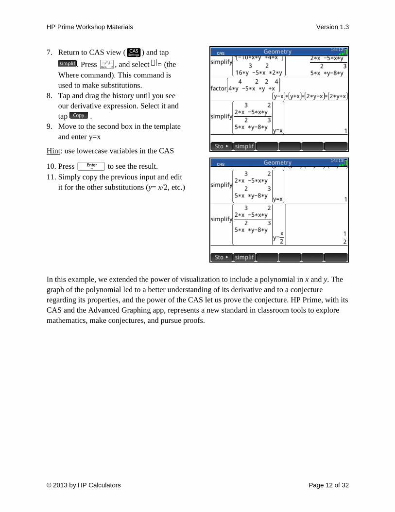
7. Return to CAS view (K) and tap
. Press F, and select (the
Where command). This command is
used to make substitutions.
8. Tap and drag the history until you see
our derivative expression. Select it and
tap .
9. Move to the second box in the template
and enter y=x
Hint: use lowercase variables in the CAS
10. Press E to see the result.
11. Simply copy the previous input and edit
it for the other substitutions (y= x/2, etc.)
In this example, we extended the power of visualization to include a polynomial in x and y. The
graph of the polynomial led to a better understanding of its derivative and to a conjecture
regarding its properties, and the power of the CAS let us prove the conjecture. HP Prime, with its
CAS and the Advanced Graphing app, represents a new standard in classroom tools to explore
mathematics, make conjectures, and pursue proofs.
HP Prime Workshop Materials Version 1.3
© 2013 by HP Calculators Page 13 of 32
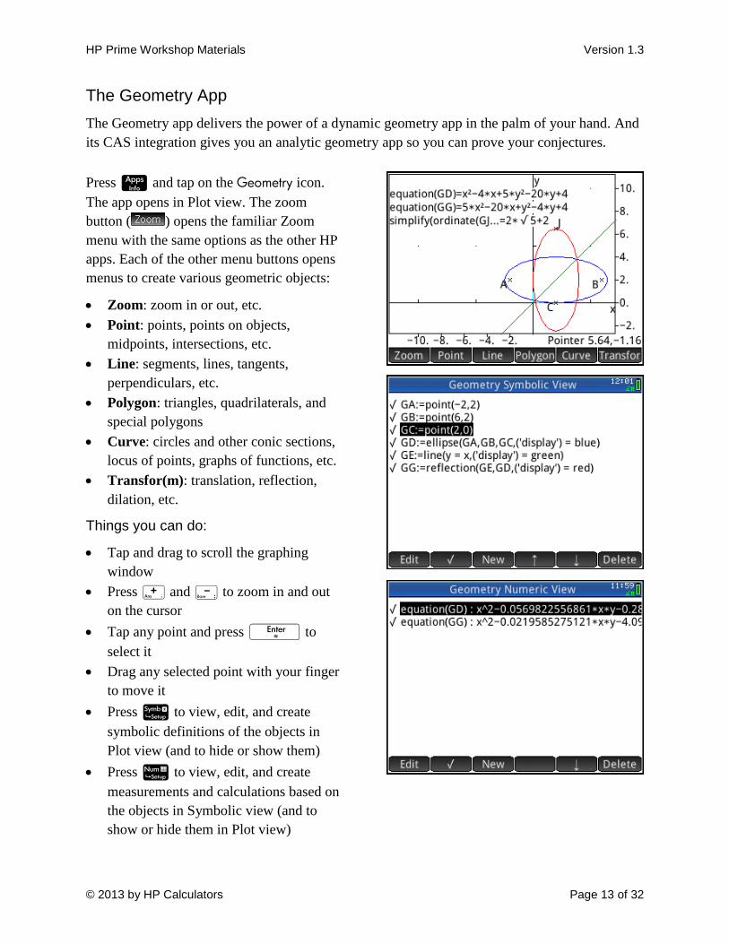
The Geometry App
The Geometry app delivers the power of a dynamic geometry app in the palm of your hand. And
its CAS integration gives you an analytic geometry app so you can prove your conjectures.
Press I and tap on the Geometry icon.
The app opens in Plot view. The zoom
button ( ) opens the familiar Zoom
menu with the same options as the other HP
apps. Each of the other menu buttons opens
menus to create various geometric objects:
Zoom: zoom in or out, etc.
Point: points, points on objects,
midpoints, intersections, etc.
Line: segments, lines, tangents,
perpendiculars, etc.
Polygon: triangles, quadrilaterals, and
special polygons
Curve: circles and other conic sections,
locus of points, graphs of functions, etc.
Transfor(m): translation, reflection,
dilation, etc.
Things you can do:
Tap and drag to scroll the graphing
window
Press + and w to zoom in and out
on the cursor
Tap any point and press E to
select it
Drag any selected point with your finger
to move it
Press Y to view, edit, and create
symbolic definitions of the objects in
Plot view (and to hide or show them)
Press M to view, edit, and create
measurements and calculations based on
the objects in Symbolic view (and to
show or hide them in Plot view)

HP Prime Workshop Materials Version 1.3
© 2013 by HP Calculators Page 14 of 32
Example 1: Exploring Quadrilaterals
In this activity, we use the Geometry app to create a quadrilateral. We then create and connect
the midpoints of consecutive sides of the quadrilateral to form another quadrilateral and explore
the properties of the latter in terms of the former.
1. Press I and tap the Geometry icon.
The app opens in its Plot view.
2. Tap and select 2Quadrilateral.
3. Tap a location and press E to
select the first vertex of the quadrilateral.
Continue to tap and press E to
select the other three vertices. Press J
to deselect the quadrilateral command.
The display now shows a quadrilateral
named E, based on the four points A, B, C,
and D.
4. Tap and select 3Midpoint. Tap near
the midpoint of ____
AB and press E .
Continue likewise to create the
midpoints of the other segments. When
you are done, press J to deselect the
midpoint command.
5. Repeat Steps 2 and 3 to create
quadrilateral O from points K, L, M, and
N.
The display now shows both quadrilaterals.
We will now tidy up our construction and
making it colorful before beginning our
explorations.
6. Press Y to display the Symbolic view
of the app. Here, each of the geometric
objects is defined symbolically. Objects
with checks besides them are displayed
in the Plot view. Uncheck each segment
by highlighting it and pressing .
Scroll down to uncheck the segments
KL, LM, MN, and NK as well.

HP Prime Workshop Materials Version 1.3
© 2013 by HP Calculators Page 15 of 32
7. With the segments hidden, return to the
Plot view (press P ) and give the
quadrilaterals their own colors. Press
Z to open the context-sensitive menu
and select 3Change Color. A choose box
pops up with the various geometric
objects. Tap on GE:=quadrilateral(GA,…;
then tap on the red box in the color
picker.
8. Repeat Step 7 to select dark blue for the
inner quadrilateral. You will have to
drag with your finger to scroll down the
choose box of objects to locate
GO:=quadrilateral(GK,….
9. Press M to open the Numeric view of
the app. Here we define measurements
and tests involving our geometric
objects. Tap to start a new
measurement. In this case, it is a test.
Tap to open the menu of
commands select 2Tests, then select
Ais_parallelogram. The command is pasted
into the command line. Remember that
the name of our inner quadrilateral is
GO. Type “GO” between the
parentheses and press E . Tap
to check this test for display in the
Plot view.
10. Return to the Plot view to see our
constructions and the test result. Drag
anywhere outside of the construction to
pan the plane so you can see both the
test result and the construction.
We are now ready to explore our
construction.

HP Prime Workshop Materials Version 1.3
© 2013 by HP Calculators Page 16 of 32
1. Select one of the vertices of the outer
quadrilateral by tapping on it and
pressing E . You can now drag it
anywhere within the display with your
finger. As you move a vertex, notice that
the parallelogram test on KLMN
maintains a value of 1, indicating it is
always a parallelogram. The
parallelogram test can return any of 5
values:
0. Not a parallelogram
1. A parallelogram only
2. A rhombus
3. A rectangle
4. A square
You can now explore by dragging, but there
is also another way to explore the effects of
the properties of ABCD on KLMN.
2. Press Y to return to the Symbolic
view. Here you can give the coordinates
of points A, B, C, and D exact values.
3. Select GA, tap and enter new
coordinates (-3,3). Tap when you
are done.
4. Repeat Step 3 with points B, C, and D so
that you have A(-3,3), B(3,3), C(3,-3)
and D(-3,-3), making ABCD a square.
5. Press P to return to the Plot view. The
display shows the parallelogram test
now has a value of 4, indicating that
KLMN is a square as well.

HP Prime Workshop Materials Version 1.3
© 2013 by HP Calculators Page 17 of 32
It seems that KLMN is always at least a
parallelogram, no matter where we move the
coordinates of points A, B, C, and D (as
long as they are not collinear!). To see why
this is so, simply construct the diagonals AC
and BD.
6. Tap and select 1Segment. Tap on
point A and press E . Then tap on
Point C and press E . Repeat with
points B and D. Then press J to
deselect the command.
Since segment KL joins the midpoints of
two sides of ΔABC, then it is parallel to the
third side (AC); likewise, MN joins the
midpoints of two sides of ΔACD, and is thus
parallel to AC as well. Thus KL and MN are
parallel. The same can be seen for segments
NK and ML.
7. Press I and tap to save your
construction with a name you’ll
remember
With the testing and symbolic abilities of the
Geometry app, students can set about the
proofs or refutations of conjectures such as
these:
If ABCD is a rhombus, then KLMN is a
rectangle
If ABCD is a rectangle, then KLMN is a
rhombus
If ABCD is an isosceles trapezoid, then
KLMN is a rhombus
If the diagonals of ABCD are
perpendicular, then KLMN is a rectangle
If the diagonals of ABCD are congruent,
then KLMN is a rhombus

HP Prime Workshop Materials Version 1.3
© 2013 by HP Calculators Page 18 of 32
Example II: Slope and Derivative of a Function
In this activity, we construct a visualization tool for the derivative of a function.
1. With your previous construction saved,
press I, use the direction keys to
select the Geometry icon, and tap .
You will be asked to confirm the reset;
tap .
2. Tap , tap 6Plot, and select
1Function. If there are any functions
defined in the Function app, a window
pops up asking if you want to use any of
them or create a new one. Select New.
3. An editor opens with plotfunc( and new
menu buttons appear with x and y. Enter
the function 1322
23
xxx
after the
parenthesis and tap . The graph of
the function is drawn. Press + to
zoom in.
Note: the Geometry app uses lowercase x as
the independent variable for functions.
4. Tap and select 2Point On. Tap on
the graph (it will turn blue when
selected) and press E. Point B
appears, defined as a point on the graph.
Press J to exit this command.
5. Tap , tap 5More , and select 5Tangent. Tap on the curve and press
E. Then tap on point B. A
message at the bottom should read
tangent(GA,GB). Press E. The
tangent to the function through point B
is drawn.

HP Prime Workshop Materials Version 1.3
© 2013 by HP Calculators Page 19 of 32
6. Tap point B and press E to select
it. You can now drag point B along the
curve with your finger or tap on a new
location and the tangent line will follow.
7. Press Y to see the Symbolic view of
the app. All objects created in the Plot
view have their symbolic definitions
here.
8. Tap to create new object. Tap
, tap 1Point, and select
5Point. The
point() command appears in the edit line.
We will now define the coordinates of this
point. The x-coordinate will be the same as
that of point B and the y-coordinate will be
the same as the slope of the tangent. The
new point D will be a point on the derivative
of the function.
9. Press D and tap to open the
Catalog. Press A a to jump to
commands that start with A and find
abscissa. Tap . Between the
parentheses, type GB. Move past the
right parenthesis, press o and return
to the Catalog for the slope and tangent
functions. The completed definition is
shown to the right.
10. Press P to return to Plot view. As
you move point B, you can see that point
D moves along the derivative.
We are now ready to use our construction!

HP Prime Workshop Materials Version 1.3
© 2013 by HP Calculators Page 20 of 32
1. Return to Symbolic view and create a
new object, GE. As shown to the right,
GE:=trace(GD).
2. Return to Plot view, select point B and
move it. Each time you tap the display to
move point B, a small marker will be left
to show where point D was. As you
continue to tap, the shape of the
derivative function emerges, as shown to
the right.
3. Uncheck GE in Symbolic view to erase
the trace and keep it from drawing in
Plot view
4. Return to Symbolic view and create GF.
Define GF:=locus(GD,GB), which means
the locus of point D as point B moves
along the graph. This new object
represents the derivative function, as
shown right and below. Check and
uncheck it in Symbolic view to show
and hide it in Plot view.
You now have a construction that has a
number of methods to visualize the
derivative of a function:
Move point B and see a single point
on the derivative that has the same x-
value as point B
Move point B and leave a trace of
points on the derivative
View the entire locus of points on
the derivative
As you can see from the figure to the right,
you can return to Symbolic view and change
GA to be the graph of any function. The
trace and locus will continue to work. Your
students can now visualize the graph of the
derivative of any function using this one
construction. Save your construction now
with a name you will remember!

HP Prime Workshop Materials Version 1.3
© 2013 by HP Calculators Page 21 of 32
Example III: Reflection and Inverse
In this construction, we have a blue ellipse defined
by the focal points A and B, and a point C on the
ellipse. The red ellipse is the reflection of the blue
one over the line y=x, so they are inverses of each
other. Note the equations of the two ellipses and
how the roles of x and y are interchanged. Since
the points A, B, and C were defined exactly in the
Symbolic view, the equations are exact as well.
Also, the y-coordinate of point J is shown to
emphasize the exact nature of the result.
1. With your previous construction saved,
reset the Geometry app
2. Tap and select 2Ellipse. Tap at the
location of the first focus and press
E. Then proceed with the second
focus and a point on the ellipse. Press
+ to zoom in and drag to scroll the
window. Change the color of your
ellipse to blue.
3. In Symbolic view, create GE:=line(y=x)
4. Back in Plot view, tap and select 2Reflection. Tap the line and press
E. Then tap the ellipse and press
E. Each time you select an
object, it should turn light blue to
indicate it is selected. Press J to exit
the reflection command. Change the
color of the reflected ellipse to red.

HP Prime Workshop Materials Version 1.3
© 2013 by HP Calculators Page 22 of 32
The Numeric view of the Geometry app is
where you go to make measurements or
create calculations based on measurements.
Check the ones you want displayed in the
Plot view.
5. Press M to see Numeric view. Tap
to create a new measurement or
calculation. Tap to open the
Commands menu, tap 1Measure, and
select Bequation. After the parentheses,
type GD (the name of the first ellipse)
and tap .
6. Repeat Step 5 to get the equation of the
reflected ellipse (GG)
7. Check both entries in Numeric view to
ensure that they are visible in Plot view.
Note the approximate nature of the
equations.
8. Return to Symbolic view and change the
coordinates of points A, B, and C as
shown to the right above.
9. Now when you return to Plot view, the
equations are shown exactly.
You can see that the roles of x and y are
interchanged in the two equations. Note also
that the y-coordinate of Point J is reported as
an exact value as well. The CAS can be used
to retrieve the equation of the red ellipse and
put it into a more familiar form. Note the
length of the major semi-axis is 5220
and the center is at (2,2). So the point J on
the reflected ellipse should have a y-
coordinate of 522 , which it does! The
integration of CAS and dynamic geometry
gives you an exact analytical geometry app
that is dynamic as well.

HP Prime Workshop Materials Version 1.3
© 2013 by HP Calculators Page 23 of 32
The Spreadsheet App
The Spreadsheet App gives you the most common features you expect in a spreadsheet. But with
HP Prime, you also get the power of a CAS integrated with the spreadsheet.
Press I and tap the Spreadsheet icon. The
app opens in Numeric view-its only view.
The menu keys are:
Format: opens the Format menu (see
figure to the right and below)
Go To: jumps to a specified cell
Select: activates Selection mode
Go: determines which cell is selected
when you tap
Show: displays the cell contents in
textbook format
Things you can do:
Tap and drag to scroll through the
spreadsheet
Tap and hold to invoke Selection mode;
then drag to select a rectangular block of
cells
Pinch open or closed horizontally to
change the width of a column
Pinch open or closed vertically to change
the height of a row
Enter contents into a cell (number,
matrix, expression
Define a cell, row, column or sheet using
a formula
The Spreadsheet app can return numerical
approximations for a formula, or it can use
the CAS to return exact numeric or symbolic
results. The examples in this section will
cover both uses.
HP Prime Workshop Materials Version 1.3
© 2013 by HP Calculators Page 24 of 32
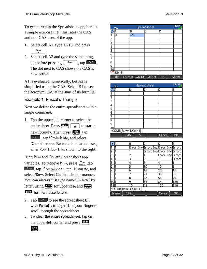
To get started in the Spreadsheet app, here is
a simple exercise that illustrates the CAS
and non-CAS uses of the app.
1. Select cell A1, type 12/15, and press
E.
2. Select cell A2 and type the same thing,
but before pressing E, tap .
The dot next to CAS shows the CAS is
now active
A1 is evaluated numerically, but A2 is
simplified using the CAS. Select B1 to see
the acronym CAS at the start of its formula.
Example 1: Pascal’s Triangle
Next we define the entire spreadsheet with a
single command.
1. Tap the upper-left corner to select the
entire sheet. Press S . to start a
new formula. Then press D ,tap
, tap 5Probability, and select 3Combinations. Between the parentheses,
enter Row-1,Col-1, as shown to the right.
Hint: Row and Col are Spreadsheet app
variables. To retrieve Row, press a,tap
, tap 1Spreadsheet , tap 1Numeric, and
select 3Row. Select Col in a similar manner.
You can always just type names in letter by
letter, using A for uppercase and A
S for lowercase letters.
2. Tap to see the spreadsheet fill
with Pascal’s triangle! Use your finger to
scroll through the spreadsheet.
3. To clear the entire spreadsheet, tap on
the upper-left corner and press S
J.

HP Prime Workshop Materials Version 1.3
© 2013 by HP Calculators Page 25 of 32
Example II: The Fibonacci Sequence
Another important variable for the
Spreadsheet app is Cell, as you will see in
our next example.
1. Tap on the column header for Column A
to select it.
2. Press S . to start a new formula.
Then enter Cell(Row-2,1)+Cell(Row-1,1)
as shown to the right.
3. Tap to see Column A fill with
zeroes.
4. But now enter 1 in cell A1 to see
Column A fill with the Fibonacci
sequence.
You can now appreciate the value of the app
variables, Cell, Col, and Row!
Example III: Back to Pascal’s Triangle
Here is another CAS example that involves
symbolic results.
In the example to the right, we use the CAS
to define one column of the spreadsheet to
expand the binomial x+1 to various integer
powers. Note the expression editor shows a
CAS button: . When active, the CAS
is used to evaluate the formula. When it is
not active, the formula is used to obtain
numerical results.
Imagine all the patterns you and your
students can explore in symbolic
expressions!

HP Prime Workshop Materials Version 1.3
© 2013 by HP Calculators Page 26 of 32
Examination Mode
HP Prime can be configured and locked for an examination. The machine will remain locked for
a pre-set time period and secured with a password. LED lights at the top of the unit will flash to
show that it is in examination mode.
1. Press S H to enter Home Settings
2. Swipe upwards to get to the third page;
the header will say Exam Mode.
Alternately, press the right halves of
and .
The menu keys are:
Config: opens the Configuration page,
where you can check which features you
want disabled
Choose: opens a choose box
Page: tap the left help to go up a page
and the right half to go down a page in
the Home Settings
More: opens a menu of options to copy
or reset the current configuration
Start/Send: starts Exam mode on the
current HP Prime or send it to another
HP Prime (Start changes to Send if
Prime is connected via USB)
Things you can do:
Give your configuration a name
Set a time period
Set a password
Check a box to erase memory when
examination mode starts
Check a box to make the LED lights
blink while in examination mode.

HP Prime Workshop Materials Version 1.3
© 2013 by HP Calculators Page 27 of 32
3. Tap Configuration, tap , and enter
a name for our new configuration:
EXAM2014
4. Tap Timeout, then tap and select a
time period.
5. Tap Default Angle, then tap and
select a default angle measure
6. Tap Blink LED twice (to select it and
check it)
We are now ready to define our EXAM2014
configuration.
7. Tap to enter the Configuration
page
8. Tap User Apps to disable saved apps
with their data
9. Tap CAS to disable the CAS
10. Tap New Notes and Programs to disable
the Note and Program editors
11. Tap and drag to scroll down the tree
12. Tap on the plus sign (+) next to
Mathematics to expand the tree
13. Tap on Hyperbolic to disable all
hyperbolic trigonometric functions
14. Tap on the plus sign next to Probability
to expand the tree another level and tap
COMB and PERM to disable the
individual functions nCr and nPr
15. Tap to save this configuration
with your new name: EXAM2014
16. Press to start Exam Mode on the
device, or if it is connected to another
HP Prime, press to start Exam
Mode on the attached HP Prime
Once Exam Mode starts, the LED lights will
blink to show that the configuration is in
effect. All HP Prime calculators that were
sent the same Exam Mode configuration
from the same HP Prime will blink in unison
using a random pattern of the 3 color lights.

HP Prime Workshop Materials Version 1.3
© 2013 by HP Calculators Page 28 of 32
The Data Streamer App
The Data Streamer App works with the HP StreamSmart 410 and up to four Fourier® sensors to
collect data in real time. The final data set is sent to one of the statistics apps for analysis. Just
plug 1-4 sensors into the StreamSmart 410 and start the Data Streamer App.
Press I and tap the DataStreamer icon.
The app opens in Plot view. The menu keys
are:
Chan: select one of the 4 channels for
tracing (if more than one sensor is
connected)
Pan/Zoom: select whether the direction
keys are used to Pan (scroll) or Zoom the
Plot view
Trace: toggles tracing off and on
Scope: start oscilloscope mode
Export: opens a menu to select data to
export to a statistics app for analysis
Start/Stop: starts and stops data
streaming
: displays a second page of options
Things you can do:
With Pan active, press = and \ to
move the current data stream up and
down in the Plot view
Tap to change it to . Press
> and < to zoom in or out on the Plot
view while data is streaming. The effect
is to speed up or slow down the data
stream until it meets your needs.
Tap to stop data streaming. It
changes to , ready for you to start
another data stream
Tap to open the Export menu,
where you can select just the data you
want and send it to one of the Statistics
apps for analysis

HP Prime Workshop Materials Version 1.3
© 2013 by HP Calculators Page 29 of 32
Example: Temperature Experiment
In this example, we plunge a temperature sensor into a beaker of ice water.
1. Attach a temperature sensor to the
StreamSmart 410, and attach the
StreamSmart 410 to your HP Prime via
the USB cable
2. On the HP Prime, Press I and tap the
DataStreamer icon
3. Tap to begin data streaming
4. While streaming and with Pan active (
), press = and \ to center the
data stream in the display
5. Tap to change it to . Now
press = and \ to zoom in and out
vertically so the stream fits in the display
6. When you see the data you want, tap to
stop data streaming
7. Tap to open the Export menu.
8. Tap and press > and < to
crop data from the left
9. When you have selected the data you
want, tap and . Tap
again to start the Statistics 2Var app with
your data.
10. Press Y to enter the Symbolic view.
Tap on Type1, tap and select
Exponential.
11. Press V and select Autoscale to see
the scatter plot of your data and the
exponential fit.
12. Press Y to return to the Symbolic
view to see the equation of your fit

HP Prime Workshop Materials Version 1.3
© 2013 by HP Calculators Page 30 of 32
The HP Prime Connectivity Kit
The HP Connectivity Kit allows you to connect to one or more HP Prime calculators via USB or
wirelessly.
The Connectivity Kit has three panes:
Calculator Pane: see the data on the connected calculator, edit apps, write programs, and
synchronize the new data with the connected HP Prime calculator
Content Pane: create and edit Exam Mode configurations, create polls and quizzes, etc.
Class pane: see all HP Prime displays in your classroom network, monitor students, send
apps, data, polls, quizzes, share one student’s display for discussion purposes, send and
start an Exam Mode configuration to the entire class, etc.

HP Prime Workshop Materials Version 1.3
© 2013 by HP Calculators Page 31 of 32
Appendix
Example: Local Linearity, the Difference Quotient and Limits
This activity uses the Function App in a split-screen view to explore the basic concept of local
linearity and the limit of the difference quotient as underpinning the notion of derivative.
11. Press I and tap the Function icon.
The app opens in its Symbolic view.
12. Enter )sin()(1 XXF and
0
)0(1)(1)(2
X
FXFXF as shown to
the right. We use “X-0” in the
denominator to reflect the difference
quotient and to allow extensions.
13. Press V and select Split Screen: Plot
Table. Press 0 E to create a row in
the table at x=0, then press \ to trace
F2(X). The table shows the value of
F2(0) as undefined. The cursor appears
to remain on F1(0), since the value of
F2(0) is not defined.
14. Press + to zoom in on the graph of
F1(X) at x=0.
As you continue to press + to zoom in,
you are zooming in on both the graph of
F1(X) at x=0 and the row of the F2(X)-
values where x=0. Connecting both of these
simultaneously helps students see that:
F1(X) begins to exhibit local linearity
near x=0
The slope of F1(X) near x=0 appears to
be converging to 1 as a limit

HP Prime Workshop Materials Version 1.3
© 2013 by HP Calculators Page 32 of 32
Example: Color blending with multiple relations plotted in the Advanced Graphing app
The graphic below was created using 4 relations plotted in the Advanced Graphing app. It shows
how color blending is used with multiple relations in the app. Change the color of each relation
and observe the effect on the graph. The relations are shown below. If you are using the HP
Prime virtual calculator, you can copy and paste them easily.
S1:
(SIN((π/LN(2))*LN(√(X^2+Y^2)*(3*COS(((ATAN(X/Y)+(π/12))MOD(π/4))-
(π/8))+√(9*COS(((ATAN(X/Y)+(π/12))MOD(π/4))-(π/8))^2-
8))))*SIN((π/LN(2))*LN(√(X^2+Y^2)*(3*COS(((ATAN(X/Y)+(π/12))MOD(π/4))-(π/8))-
√(9*COS(((ATAN(X/Y)+(π/12))MOD(π/4))-(π/8))^2-8)))))<0
S2:
(SIN((π/LN(2))*LN(√(X^2+Y^2)*(3*COS(((ATAN(X/Y)+(-π/12))MOD(π/4))-
(π/8))+√(9*COS(((ATAN(X/Y)+(-π/12))MOD(π/4))-(π/8))^2-
8))))*SIN((π/LN(2))*LN(√(X^2+Y^2)*(3*COS(((ATAN(X/Y)+(-π/12))MOD(π/4))-(π/8))-
√(9*COS(((ATAN(X/Y)+(-π/12))MOD(π/4))-(π/8))^2-8)))))<0
S3:
(SIN((π/LN(2))*LN(√(X^2+Y^2)*(3*COS(((ATAN(X/Y)+(0/12))MOD(π/4))-
(π/8))+√(9*COS(((ATAN(X/Y)+(0/12))MOD(π/4))-(π/8))^2-
8))))*SIN((π/LN(2))*LN(√(X^2+Y^2)*(3*COS(((ATAN(X/Y)+(0/12))MOD(π/4))-(π/8))-
√(9*COS(((ATAN(X/Y)+(0/12))MOD(π/4))-(π/8))^2-8)))))<0
S4:
(SIN((((π/LN(2))))*LN(2*√(X^2+Y^2)*(6*COS(ATAN((((MIN(ABS(X),ABS(Y))/MAX(ABS(X),ABS(Y)))))))+√(3
6*COS(ATAN((((MIN(ABS(X),ABS(Y))/MAX(ABS(X),ABS(Y)))))))^2-
27))))*SIN((((π/LN(2))))*LN(2*√(X^2+Y^2)*(6*COS(ATAN((((MIN(ABS(X),ABS(Y))/MAX(ABS(X),ABS(Y))))))
)-√(36*COS(ATAN((((MIN(ABS(X),ABS(Y))/MAX(ABS(X),ABS(Y)))))))^2-27)))))<0