• Introduction• Detecting Faces in a Single Image– Knowledge-Based Methods– Feature-Based Methods– Template Matching– Appearance-Based Methods

• Face Image Database• Performance Evaluation

• Face detection– Determining whether or not there are

any faces on the image and, if present, return the image location and extent of each face

Extent of face

Location of face

• Problems for Face Detection– Pose– Presence or absence of structural

components– Facial expression– Occlusion– Image orientation– Image conditions

• Related Problems of Face detection

Face localization : determine the image position of a single face, with the assumption that an input image contains only one face

Facial feature detection : detect the presence and location of features, such as eyes, nose, nostrils, eyebrow, mouth, lips, ears, etc.

Face recognition of face identification : compares an input image against a database and reports a match

Face authentication : verify the claim of the identity of an individual in an input image

Face tracking : continuously estimate the location and possibly the orientation of a face in an image sequence in real time.

Facial expression recognition : identify the affective states (happy, sad, disgusted, etc.) of humans

• Four categories of detection methods

1. Knowledge-based methods : use known human prior knowledge

2. Feature invariant approaches : aim to find structural features that exist even when the pose, viewpoint, or lighting conditions vary, and then use the these to locate faces.

3. Template matching methods : Several standard patterns of a face are stored to describe the face as a whole or the facial features separately.

4. Appearance-based methods : learn models or templates from a set of training images

• Human-specified rules– A face often appears in an image with two eyes that are

symmetric to each other, a nose, and a mouth.

– The relationships between features can be represented by their relative distances and positions.

– Facial features in an input image are extracted first, and face candidates are identified based on the coded rules.

– A verification process is usually applied to reduce false detections.

• Difficulties if these methods– The trade-off of details and extensibility

– It is hard to enumerate all possible cases. On the other hand, heuristics about faces work well in detecting frontal faces in uncluttered scenes.

• Three levels of rules

– All possible face candidates are found by scanning a window over the input image.

– A rules at a higher level are general descriptions of what a face looks like.

– The rules at lower levels rely on details of facial features.

• Rules at the lowest resolution (Level 1)– The part of the face has four cells with a basically uniform

intensity. – The upper round part of a face has a basically uniform

intensity. – The difference between the average gray values of the center

part and the upper round part is significant.

• The lowest resolution image is searched for face candidates and these are further processed at finer resolutions.

• Rules at the Level 2– Local histogram equalization is performed on the face

candidates, followed by edge detection

• Rules at the Level 3– Detail rules of eyes and mouth.

• Use horizontal and vertical projections of the pixel intensity.

• The horizontal profile of an input image is obtained first, and then the two local minima may correspond to the left and right side of the head.

• The vertical profile is obtained the local minima are determined for the locations of mouth lips, nose tip, and eyes.

• Have difficulty to locate a face in a complex background

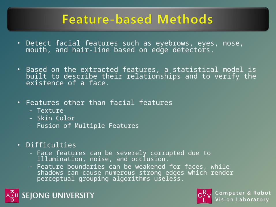
• Detect facial features such as eyebrows, eyes, nose, mouth, and hair-line based on edge detectors.

• Based on the extracted features, a statistical model is built to describe their relationships and to verify the existence of a face.

• Features other than facial features– Texture– Skin Color– Fusion of Multiple Features

• Difficulties– Face features can be severely corrupted due to illumination,

noise, and occlusion.– Feature boundaries can be weakened for faces, while shadows

can cause numerous strong edges which render perceptual grouping algorithms useless.

• Sirohey 1993:– Use an edge map (Canny detector) and heuristics to remove and

group edges so that only the ones on the face contour are preserved.

– An ellipse is then fit to the boundary between the head region and the background.

• Chetverikov and Lerch 1993:– Use blobs and streaks (linear sequences of similarly oriented

edges).– Use two dark blobs and three light blobs to represent eyes,

cheekbones and nose.– Use streaks to represent the outlines of the faces, eyebrows and

lips.– Two triangular configurations are utilized to encode the spatial

relationship among the blobs.– Procedure:

• A low resolution Laplacian image is gnerated to facilitate blob detection.• The image is scanned to find specific triangular occurences as candidates• A face is detected if streaks are identified around a candidate.

• Graf et. al. 1995:– Use bandpass filtering and morphological operations

• Leung et. al. 1995:– Use a probabilistic method based on local feature detectors and random

graph matching

– Formulate the face localization problem as a search problem in which the goal is to find the arrangement of certain facial features that is most likely to be a face patter.

– Five features (two eyes, two nostrils, and nose/lip /junction).

– For any pair of facial features of the same type, their relative distance is computed and modeled by Gaussian.

– Use statistical theory of shape (Kendall1984, Mardia and Dryden 1989), a joint probability density function over N feature points, for the i th feature under the assumption that the original feature points are positioned in the plane according to a general 2N-dim Gaussian.

• Yow and Cipolla 1996:– The first stage applies a second derivative Gaussian filter, elongated at an

aspect ratio of three to one, to a raw image.

– Interest points, detected at the local maxima in the filter response, indicate the possible locations of facial features.

– The second stage examines the edges around these interest points and groups them into regions.

– Measurements of a region’s characteristics, such as edge length, edge strength, and intensity variance are computed and stored in a feature vector.

– Calculate the distance of candidate feature vectors to the training set.

– This method can detect faces at different orientations and poses.

• Augusteijn and Skufca 1993:

– Use second-order statistical features on submiages of 16x16 pixels.

– Three types of features are considered: skin, hair, and others.

– Used a cascade correlation neural network for supervised classifications.

• Dai and Nakano1996:

– Use similar method + color

– The orange-like parts are enhanced.

– One advantage is that it can detect faces which are not upright or have features such as beards and glasses.

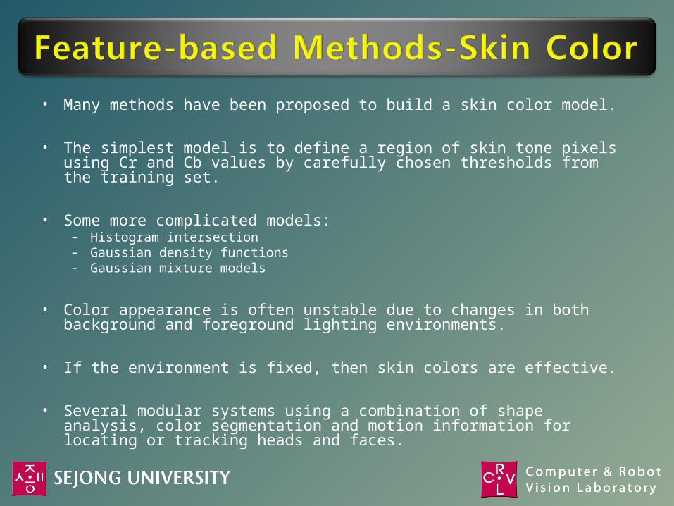
• Many methods have been proposed to build a skin color model.

• The simplest model is to define a region of skin tone pixels using Cr and Cb values by carefully chosen thresholds from the training set.

• Some more complicated models:– Histogram intersection– Gaussian density functions– Gaussian mixture models

• Color appearance is often unstable due to changes in both background and foreground lighting environments.

• If the environment is fixed, then skin colors are effective.

• Several modular systems using a combination of shape analysis, color segmentation and motion information for locating or tracking heads and faces.

• A standard face pattern (usually frontal) is manually predefined or parameterized by a function.

• Given an input image, the correlation values with the standard patterns are computed for the face contour, eyes, nose and mouth independently.

• The existence of a face is determined based on the correlation values.

• Advantage: simple to implement.

• Disadvantage: need to incorporate other methods to improve the performance

• Sinha 1994:– Designing the invariant based on

the relations of regions.

– While variations in illumination change the individual brightness of different parts of faces remain large unchanged.

– Determine the pairwise ratios of the brightness of a few such regions and record them as a template.

– A face is located if an image satisfies all the pairwise brighter-darker constraints.

• Supervised learning• Classification of face / non-face• Methods:– Eigenfaces– Distribution-based Methods– Neural Networks– Support Vector Machines– Sparse Network– Naive Bayes Classifier– Hidden Markov Model

• Apply eigenvectors in face recognition (Kohonen 1989).

– Use the eigenvectors of the image’s autocorrelation matrix.

– These eigenvectors were later known as Eigenfaces.

• Images of faces can be linearly encoded using a modest number of basis images.

• These can be found based on the K-L transform or Principal component analysis (PCA).

• Try to find out a set of optimal basis vector eigenpictures.

• Sung and Poggio 1996:– Each face and nonface example is normalized to a

19x19 pixel image and treated as a 361- dimensional vector or pattern.

– The patterns are grouped into six face and six nonface clusters using a modified k-means algorithm.

• Rowley 1996:– The first component is a neural network that

receives a 20 x 20 pixel region and outputs a score ranging from -1 to 1.

– Nearly 1050 face samples are used for training.

• The goal of training an HMM is to maximize the probability of observing the training data by adjusting the parameters in an HMM model.

• Test sets

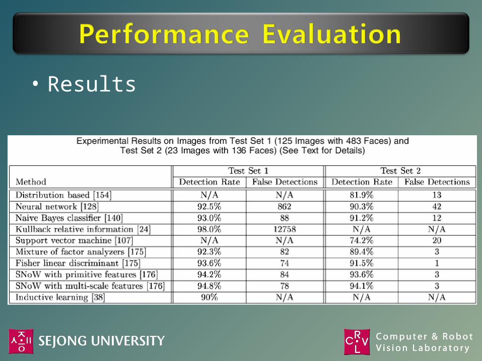
• Results