Introducing the Air Quality Life Index · Section III Introducing the Air Quality Life Index 14 ... guideline would increase average life expectancy by 2.9 and 4.3 years, respectively

Introducing the Air Quality Life IndexTwelve Facts about Particulate Air Pollution, Human Health, and Global Policy

By Michael Greenstone and Claire Qing Fan, Energy Policy Institute at the University of Chicago

NOVEMBER 2018

Index®

NEW YORK CITY 1973 NEW YORK CITY 2018

AQLI Introducing the Air Quality Life Index | 3

RUSTON, WA | EPA 1970

Table of Contents

Executive Summary 4

Section I Background on Particulate Air Pollution 6

Fact 1 Particulates are tiny and pernicious invaders of the cardiorespiratory system 7

Fact 2 Energy production is the primary source of particulate pollution 8

Fact 3 Technologies can reduce particulate pollution, but they increase energy costs 9

Section II Evidence on the Effects of Exposure 10

Fact 4 Studies link particulate pollution and health, but leave vital questions unanswered. 11

Fact 5 Latest evidence shows sustained exposure to particulate pollution leads to shorter lives 12

Section III Introducing the Air Quality Life Index 14

Fact 6 The AQLI uses hyper-localized satellite pollution measurements for the entire world 15

Fact 7 The AQLI reports the gain in life expectancy from reductions in particulate pollution 16

Section IV The AQLI at Work 18

Fact 8 Particulate pollution is the greatest global threat to human health 19

Fact 9 The average loss in life expectancy due to particulate pollution has increased from 1.0 in 1998 to 1.8 in 2016 20

Fact 10 Current particulate pollution concentrations are projected to shorten the lives of 635 million people by at least five years 21

Section V Track Record of Pollution Policies 22

Fact 11 U.S. residents are living 1.5 years longer than in 1970 thanks to reductions in particulate pollution 23

Fact 12 China is winning its “War on Pollution” 24

Appendix Data and Methodology 26

Table of Particulate Pollution and Life Expectancy Impacts by Country 30

References 34

Special thanks to Dr. Aaron van Donkelaar and the Atmospheric Composition Analysis Group at Dalhousie University for providing the satellite-derived PM2.5 raw data.

4 | Introducing the Air Quality Life Index AQLI AQLI Introducing the Air Quality Life Index | 5

EXECUTIVE SUMMARY

Particulate matter (PM) air pollution is the greatest current threat to human health globally. Its microscopic particles penetrate deep into the lungs, bypassing the body’s natural defenses. From there it can enter the bloodstream, causing lung disease, cancer, strokes, and heart attacks. There is also evidence of detrimental effects on cognition. Yet, in spite of these risks, the relationship between particulate matter air pollution levels and human health is not widely comprehended by society at large. For most people, their only insight into particulate air pollution exposure and risk is the popular Air Quality Index, which uses a color-coded system to provide a normative assessment of daily air quality. But these colors do little to convey actual health risk, and are often accompanied by measurements of units that are unfamiliar to almost everyone (e.g., micrograms of pollution per cubic meter). The Air Quality Life Index, or AQLI, represents a completely novel advancement in measuring and communicating the health risks posed by particulate matter air pollution. This is because the AQLI converts particulate air pollution into perhaps the most important metric that exists: its impact on life expectancy. The AQLI reveals that, averaged across all women, men, and children globally, particulate matter air pollution cuts global life expectancy short by nearly 2 years relative to what they would be if particulate concentrations everywhere were at the level deemed safe by the World Health Organization (WHO). This life expectancy loss makes particulate pollution more devastating than communicable

diseases like tuberculosis and HIV/AIDS, behavioral killers like cigarette smoking, and even war. Some areas of the world are impacted more than others. For example, in the United States, where there is less pollution, life expectancy is cut short by just 0.1 years relative to the WHO guideline. In China and India, where there are much greater levels of pollution, bringing particulate concentrations down to the WHO guideline would increase average life expectancy by 2.9 and 4.3 years, respectively. The AQLI is rooted in peer-reviewed research that for the first time quantified the causal relationship between long-term human exposure to air pollution and life expectancy. The Index then combines this research with hyper-localized, global PM measurements, yielding unprecedented insight into the true cost of air pollution in communities around the world. For example, the average resident of Delhi will live about 10 fewer years because of high pollution, while those in Beijing and Los Angeles will live almost six and almost one fewer years, respectively.

Beyond these factors, the AQLI stands apart in a few important respects: • The research underlying the AQLI is based on a setting with

pollution at the very high concentrations that prevail in many parts of Asia today. Previous work has relied on extrapolations of associational evidence from the low levels in the United States from cigarette studies.

• The causal nature of the AQLI’s underlying research allows it to isolate the effect of air pollution from other factors that impact health. In contrast, previous efforts to summarize the health effects of air pollution have relied on associational studies that are prone to confounding the effects of air pollution with other determinants of human health.

• The AQLI delivers estimates of the loss of life expectancy for the average person. Other approaches report the number of people who die prematurely due to air pollution, leaving unanswered by how much these lives were cut short.

• The AQLI uses highly localized satellite data, making it possible to report life expectancy impacts at the county or similar level around the world, rather than at much more aggregated levels reported in previous studies.

In addition to its importance for typical individuals around the world, the AQLI can be an invaluable tool for policymakers. It can be used to measure, track, and illustrate the impact of pollution reductions, both in terms of air quality and life expectancy. For example, reductions in air pollution resulting in large part from the Clean Air Act have added more than 1.5 years to the life expectancy of the average American since 1970. The AQLI’s data also show that, more recently, three years into a “War on Pollution,” China has achieved large reductions in air pollution. If these improvements are sustained, the average resident there would see their life expectancy increase by 0.5 years. The rest of this document lays out twelve facts about particulate air pollution and the AQLI. Section 1 provides basic background on particulate air pollution, its impacts on the human body, and its main sources. Section 2 lays out what researchers know and don’t know about particulate air pollution’s impact on health. Section 3 describes the AQLI and how it can be used. Finally, Section 4 uses the lens of the AQLI to unveil the gravity of the pollution threat to life expectancy, and where it is most severe.

Particulate matter air pollution cuts global life expectancy short by nearly 2 years


SECTION I

Background on Particulate Air PollutionParticulate matter air pollution is widely believed to be the most deadly form of air pollution. Its microscopic particles penetrate deep into the lungs and filter into the bloodstream. From there, they can eventually lead to lung disease, cancer, strokes or heart attacks. Most of this particulate pollution comes from the combustion of fossil fuels— the same fossil fuels that contribute to climate change.

FACT 1

1 Xing et al., 2016

2 E.g. Ling & van Eeden, 2009

3 Gibbens, 2018

4 Iadecola, 2013

5 Wilson & Suh, 1997

Particulates are tiny and pernicious invaders of the cardiorespiratory system. Particulate matter (PM) refers to solid and liquid particles—soot, smoke, dust, and others—that are suspended in the air. When the air is polluted with PM, these particles enter the respiratory system along with the oxygen that the body needs. After PM is breathed into the nose or mouth, each particle’s fate depends on its size: the finer the particles, the farther into the body they penetrate. PM10, particles with diameters smaller than 10 micrograms (μm), are small enough to pass through the hairs in the nose. They travel down the respiratory tract and into the lungs, where the metal elements on the surface of the particles oxidize lung cells, damaging their DNA and increasing the risk of cancer.1 The particles’ interactions with lung cells can also lead to inflammation, irritation, and blocked airflow, increasing the risk of or aggravating lung diseases that make breathing difficult, such as chronic obstructive pulmonary disorder (COPD), cystic lung disease, and bronchiectasis.2

More deadly is an even smaller classification: PM2.5 , or particles with diameter less than 2.5μm—just 3 percent the diameter of a human hair. In addition to contributing to risk of lung disease, PM2.5 particles pass even deeper into the lungs’ alveoli, the blood vessel-covered air sacs in which the bloodstream exchanges oxygen and carbon dioxide. Once PM2.5 particles enter the bloodstream via the alveoli, they inflame and constrict blood vessels or dislodge fatty plaque, increasing blood pressure or creating clots. This can block blood flow to the heart and brain, and over time, lead to stroke or heart attack. In recent years, researchers have even begun

to observe that PM pollution is associated with lower cognitive function. They speculate that PM2.5 in the bloodstream may cause the brain to age more quickly due to the inflammation. In addition, it may damage the brain’s white matter, which is what allows different regions of the brain to communicate.3 White matter damage similar to the kind linked to PM2.5 has been implicated in Alzheimer’s and dementia.4

The tiny size of PM2.5 particles not only makes them harmful from a physiological perspective, but also allows these particles to stay in the air for weeks and to travel hundreds or thousands of kilometers.5 This increases the likelihood that the particles will end up inhaled by humans before landing onto the ground.


FACT 2

6 Philip et al., 2014

7 NRC, 2010

8 Philip et al., 2014

Energy production is the primary source of particulate pollution. Though some particulates arise from natural sources such as dust, sea salt, and wildfires, most PM2.5 pollution is human-induced. The fact that burning coal pollutes the air has been known for some time. Around 1300, King Edward I of England decided that the punishment for anyone who burned coal in his kingdom would be death. Today, fossil fuel combustion not only releases carbon dioxide that increases the odds of disruptive climate change, but is also the leading global source of man-made PM2.5.6 It generates particulates through three distinct pathways7:

In addition to fossil fuel combustion, humans generate PM2.5 through the combustion of biofuels such as wood and crop residue for household cooking and heating. Biofuel burning emits black carbon and organic particulates. In many parts of the world, biofuel combustion’s contribution to particulate pollution is comparable to that of fossil fuels. The burning of biomass—forests, savannah, and crop residue on fields—to clear land for agriculture is also a significant source of anthropogenic particulate pollution.8

Figure 1 · Source Apportionment of Global Urban Ambient PM2.5

Natural Sources

Vehicles

Household Wood, Coal Burning

20%

25%

15%

22%

18%

Power Plants and Industry

Other Human Activity

Source Apportionment of Global UrbanAmbient PM2.5

Source: Karagulian et al., 2015

Because coal contains sulfur, coal-fired power plants and industrial facilities generate sulfur dioxide gas. Once in the air,

the gas may react with oxygen and then ammonia in the atmosphere to form sulfate particulates.

Combustion that occurs at high temperatures, such as in vehicle engines and power plants, releases nitrogen dioxide,

which undergoes similar chemical reactions in the air to form nitrate particulates.

Diesel engines, coal-fired power plants, and the burning of coal for household fuel all involve incomplete combustion. In this type of

combustion, not enough oxygen is present to generate the maximum amount of energy possible given the amount of fuel. Part of the

excess carbon from the fuel becomes black carbon, a component of PM2.5 that is also the second- or third-most important contribu-

tor to climate change after carbon dioxide and perhaps methane.

FACT 3

9 SO2 emissions calculated based on India 2011 estimates from Guttikunda & Jawahar (2014) and BP Statistical Review (2012), assuming 90% SO2 removal rate by FGD

10 Biondo & Marten, 1977

11 FGD costs estimated with EPIC Levelized Cost of Electricity model, based on data from U.S. EIA (2017a)

12 Calculated from U.S. EIA (2017b) and U.S. EIA (2017c)

13 U.S. EPA

14 Calculated with 2007-2008 data from U.S. EIA (2018)

15 U.S. DOE

16 Calculated from U.S. EIA (2017b) and U.S. EIA (2017c).

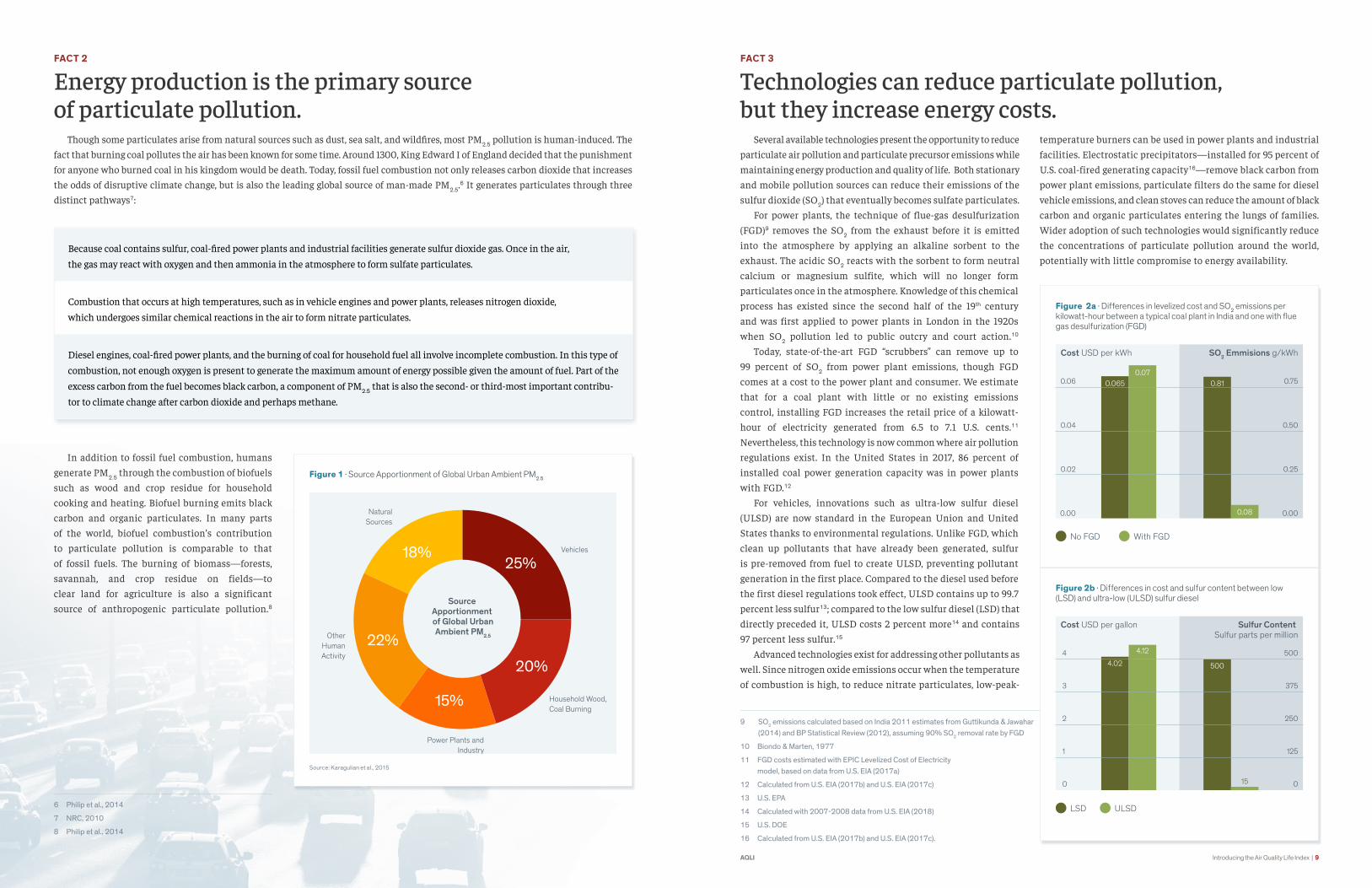
Technologies can reduce particulate pollution, but they increase energy costs. Several available technologies present the opportunity to reduce particulate air pollution and particulate precursor emissions while maintaining energy production and quality of life. Both stationary and mobile pollution sources can reduce their emissions of the sulfur dioxide (SO2) that eventually becomes sulfate particulates. For power plants, the technique of flue-gas desulfurization (FGD)9 removes the SO2 from the exhaust before it is emitted into the atmosphere by applying an alkaline sorbent to the exhaust. The acidic SO2 reacts with the sorbent to form neutral calcium or magnesium sulfite, which will no longer form particulates once in the atmosphere. Knowledge of this chemical process has existed since the second half of the 19th century and was first applied to power plants in London in the 1920s when SO2 pollution led to public outcry and court action.10 Today, state-of-the-art FGD “scrubbers” can remove up to 99 percent of SO2 from power plant emissions, though FGD comes at a cost to the power plant and consumer. We estimate that for a coal plant with little or no existing emissions control, installing FGD increases the retail price of a kilowatt-hour of electricity generated from 6.5 to 7.1 U.S. cents.11 Nevertheless, this technology is now common where air pollution regulations exist. In the United States in 2017, 86 percent of installed coal power generation capacity was in power plants with FGD.12

For vehicles, innovations such as ultra-low sulfur diesel (ULSD) are now standard in the European Union and United States thanks to environmental regulations. Unlike FGD, which clean up pollutants that have already been generated, sulfur is pre-removed from fuel to create ULSD, preventing pollutant generation in the first place. Compared to the diesel used before the first diesel regulations took effect, ULSD contains up to 99.7 percent less sulfur13; compared to the low sulfur diesel (LSD) that directly preceded it, ULSD costs 2 percent more14 and contains 97 percent less sulfur.15

Advanced technologies exist for addressing other pollutants as well. Since nitrogen oxide emissions occur when the temperature of combustion is high, to reduce nitrate particulates, low-peak-

temperature burners can be used in power plants and industrial facilities. Electrostatic precipitators—installed for 95 percent of U.S. coal-fired generating capacity16—remove black carbon from power plant emissions, particulate filters do the same for diesel vehicle emissions, and clean stoves can reduce the amount of black carbon and organic particulates entering the lungs of families. Wider adoption of such technologies would significantly reduce the concentrations of particulate pollution around the world, potentially with little compromise to energy availability.

Figure 2a · Differences in levelized cost and SO2 emissions per kilowatt-hour between a typical coal plant in India and one with flue gas desulfurization (FGD)

0.06

0.04

0.02

0.00

Cost USD per kWh

No FGD With FGD

SO2 Emmisions g/kWh

0.75

0.50

0.25

0.00

0.0650.07

0.81

0.08

Figure 2b · Differences in cost and sulfur content between low (LSD) and ultra-low (ULSD) sulfur diesel

4

3

2

1

0

Cost USD per gallon

LSD ULSD

Sulfur Content Sulfur parts per million

500

375

250

125

0

4.024.12

500

15


SECTION II

Evidence on the Effects of Exposure Scores of studies have found an association between particu-late air pollution and human health, but left open important questions on the causal impact of particulate pollution and the total loss of life expectancy. A pair of recent studies exploit a natural experiment provided by a policy in China to provide the first causal evidence on the effects of sustained exposure to particulate pollution on life expectancy. Further, they are informative about the nature of the life expectancy-particulate pollution relationship at the levels of pollution that currently prevail in Asia and other parts of the world.

FACT 4

17 Davis, 2002

18 Katsouyanni et al., 1997

19 Dockery et al., 1993

20 Chay & Dobkin, 2003; Dominici et al., 2014

Studies link particulate pollution and health, but leave vital questions unanswered. Decades of research have established strong associations between particulate pollution and various health outcomes: emergency room visits, cardiovascular and respiratory disease prevalence, and mortality. However, though valuable, these studies left a gap in our understanding of the causal impact of sustained particulate exposure on lifetime health, especially in the context of today’s industrializing countries. An extensive body of research has documented a tight link between particulates and adverse health outcomes. For example, a famous analysis suggests that the Great London Smog of 1952 killed as many as 12,000 people.17 In more recent decades as well, in European cities, days with higher particulate concentrations recorded greater numbers of deaths.18 Further, a pair of studies by Chay and Greenstone (2003a and 2003b) uncovered a robust relationship between particulate pollution and elevated infant mortality rates. Such studies go a long way towards establishing a causal relationship, but do not answer two key questions. First, how many years of life were lost across the population? It is not clear from these results whether those who die prematurely would have soon passed away from other causes, and particulate pollution may simply have exacerbated their ailments, leading to slightly sooner deaths. Second, the broader question about pollution is the impacts of exposure for many years, not just for short periods of time or while

in utero or an infant. These studies leave this second key question— what are the long-term impacts of sustained exposure —unanswered. Other research has attempted to address these questions. For example, Pope et al. (2009) found that a decrease in particulate pollution in 51 U.S. metropolitan areas from the late 1970s and early 1980s to the late 1990s and early 2000s was associated with an estimated increase in life expectancy of 0.6 years. This paper, as well as the famous Six Cities Study,19 made important progress in estimating the consequences of long-run exposure. Yet, the results of these studies are likely to be biased by confounding variables. Since people who live in more polluted places may have worse health along dimensions not measured in the data than people in less polluted places, and there may be other locational differences in the determinants of health (e.g., the quality of medical care), questions remain about whether the resulting estimates of the effects of air pollution are confounded by other factors.20

Another hole in the body of evidence is that the settings studied in most of the research are in North America and Europe, for which data is readily available but pollution levels are relatively low. As a result, the findings may not be generalizable to high-pollution settings such as China and India. Thus, there remained a need to establish the causal effects of sustained exposure to high particulate concentrations.

Figure 3 · Weekly Mortality for Greater London around Great London Smog of 1952

5000

3750

2500

1250

0

Weekly Mortality SO2 PPM

0.4

0.3

0.2

0.1

0

SO2

Weekly Mortality

Oct 18 Nov 1 Nov 15 Nov 29 Ded 13 Dec 27 Jan 10 Jan 24 Feb 7 Feb 21 Mar 7 Mar 21

Week of Great London Smog >

Source: Bell & Davis (2001)


FACT 5

21 For the conversion from the findings of Ebenstein et al. (2017) in terms of PM10 to the relationship in terms of PM2.5, see the Appendix.

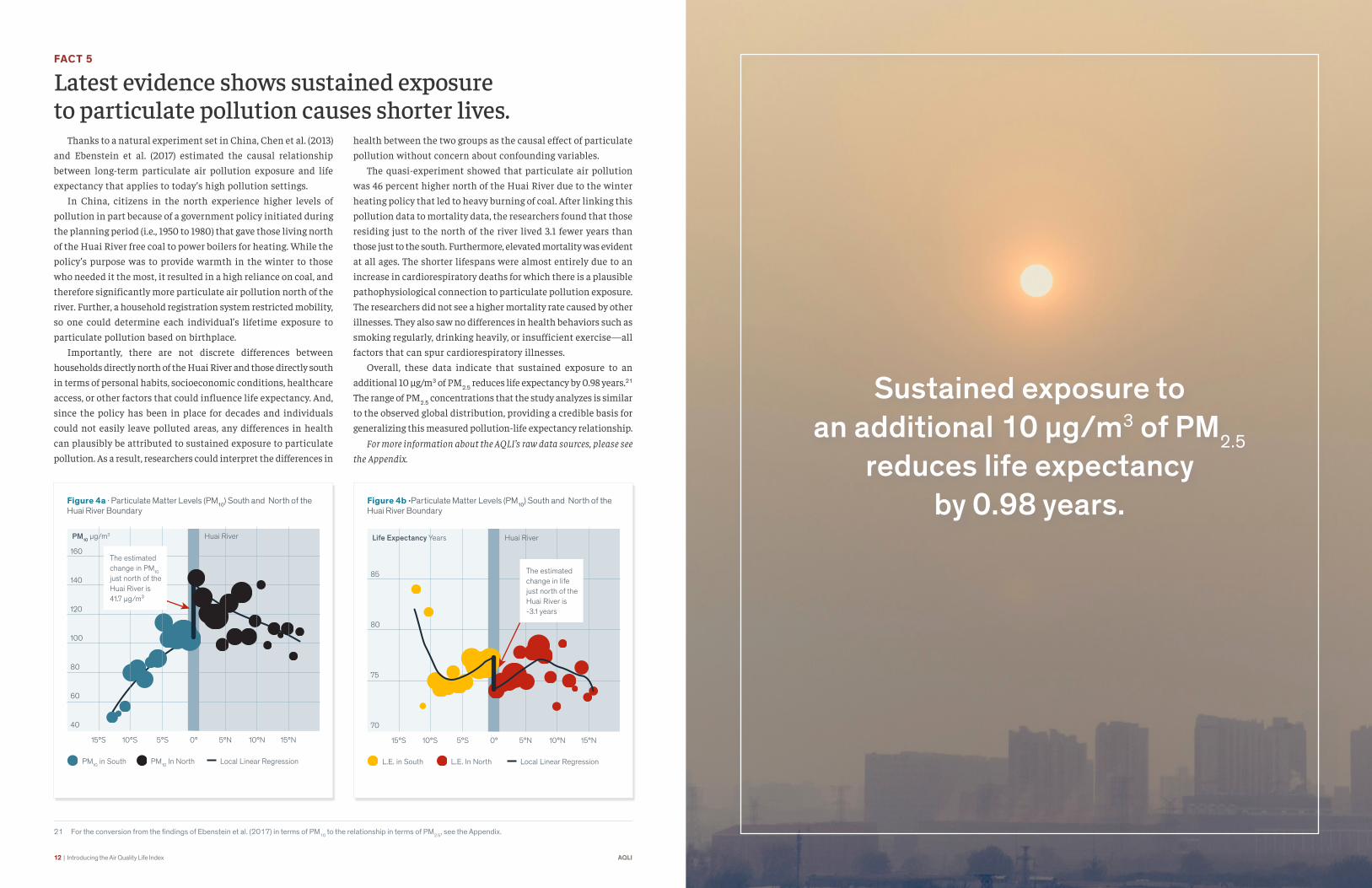
Latest evidence shows sustained exposure to particulate pollution causes shorter lives. Thanks to a natural experiment set in China, Chen et al. (2013) and Ebenstein et al. (2017) estimated the causal relationship between long-term particulate air pollution exposure and life expectancy that applies to today’s high pollution settings. In China, citizens in the north experience higher levels of pollution in part because of a government policy initiated during the planning period (i.e., 1950 to 1980) that gave those living north of the Huai River free coal to power boilers for heating. While the policy’s purpose was to provide warmth in the winter to those who needed it the most, it resulted in a high reliance on coal, and therefore significantly more particulate air pollution north of the river. Further, a household registration system restricted mobility, so one could determine each individual’s lifetime exposure to particulate pollution based on birthplace. Importantly, there are not discrete differences between households directly north of the Huai River and those directly south in terms of personal habits, socioeconomic conditions, healthcare access, or other factors that could influence life expectancy. And, since the policy has been in place for decades and individuals could not easily leave polluted areas, any differences in health can plausibly be attributed to sustained exposure to particulate pollution. As a result, researchers could interpret the differences in

health between the two groups as the causal effect of particulate pollution without concern about confounding variables. The quasi-experiment showed that particulate air pollution was 46 percent higher north of the Huai River due to the winter heating policy that led to heavy burning of coal. After linking this pollution data to mortality data, the researchers found that those residing just to the north of the river lived 3.1 fewer years than those just to the south. Furthermore, elevated mortality was evident at all ages. The shorter lifespans were almost entirely due to an increase in cardiorespiratory deaths for which there is a plausible pathophysiological connection to particulate pollution exposure. The researchers did not see a higher mortality rate caused by other illnesses. They also saw no differences in health behaviors such as smoking regularly, drinking heavily, or insufficient exercise—all factors that can spur cardiorespiratory illnesses. Overall, these data indicate that sustained exposure to an additional 10 μg/m3 of PM2.5 reduces life expectancy by 0.98 years.21 The range of PM2.5 concentrations that the study analyzes is similar to the observed global distribution, providing a credible basis for generalizing this measured pollution-life expectancy relationship.

For more information about the AQLI’s raw data sources, please see the Appendix.

Figure 4b ·Particulate Matter Levels (PM10) South and North of the Huai River Boundary

L.E. in South L.E. In North Local Linear Regression

Life Expectancy Years

85

80

75

70

15°S 5°S 0° 10°N 15°N10°S 5°N

The estimated change in life just north of the Huai River is -3.1 years

Huai River

Figure 4a · Particulate Matter Levels (PM10) South and North of the Huai River Boundary

PM10 in South PM10 In North Local Linear Regression

160

140

120

100

80

60

40

15°S 5°S 0°

Huai River

10°N 15°N10°S 5°N

The estimated change in PM10

just north of the Huai River is 41.7 µg/m³

PM10 µg/m3

Sustained exposure to an additional 10 μg/m3 of PM2.5

reduces life expectancy by 0 98 years


SECTION III

Introducing the Air Quality Life IndexThe Air Quality Life Index (AQLI) is based on the finding that an additional 10 μg/m3 of PM2.5 reduces life expectancy by 0.98 years. By combining this finding with satellite-derived, hyper-localized PM2.5 measurements around the world, the AQLI provides unprecedented insight into the global impacts of particulate pollution in local jurisdictions. The Index also illustrates how air pollution policies can increase life expectancy if pollution levels were reduced to the World Health Organization’s (WHO) safe guideline or existing national air quality standards, or by user-selected percent reductions. This information can help to inform local communities and policymakers about the benefits of air pollution policies in very concrete terms.

FACT 6

The AQLI uses hyper-localized satellite pollution measurements for the entire world. Reliable, geographically extensive pollution measurements are critical to understanding the extent of air pollution and its health impacts. Unfortunately, many areas around the world currently lack extensive pollution monitoring systems. Of the areas with monitoring, many are either newly established or did not begin monitoring PM2.5 until recently, making it impossible to track long-term impacts. The quality and trustworthiness of reported monitor data also varies, compromising comparisons of pollution across regions. To construct a single dataset of particulate pollution and its health impacts that is global in coverage, local in resolution, consistent in methodology, and that spans many years to reveal pollution trends over time, the AQLI uses satellite-derived PM2.5 measurements. From satellite images, van Donkelaar et al. (2016) were able to deduce the quantity of aerosols in the atmosphere at each location. Atmospheric composition simulations helped translate that into levels of PM2.5, which were cross-validated and interpolated using available ground-based monitor data. Finally, using the same atmospheric composition simulations, the researchers subtracted out the share of PM2.5

at each location that is due to dust and sea salt, leaving approximately the level of PM2.5 generated by human activity. The resulting dataset spans the years 1998-2016 and covers the globe at the high resolution of 10km x 10km. In other words, for every area about 1/8 the size of New York City, 1/15 the size of Delhi, or 1/40 the size of urban Beijing, it provides the annual average level of anthropogenic PM2.5 for each year over a 19 year period. Using population weights, the AQLI aggregates this data to both national and local levels. It shows, for instance, that on average, residents of Ottawa County, Ohio, in the United States and Brahmanbaria District, Chittagong, in Bangladesh were exposed to 2016 annual averages of 13.0 and 60.1 µg/m3 of PM2.5, respectively. By providing PM2.5 levels and impacts for each county-, district-, or prefecture-level area since 1998, the AQLI fills an information gap for local citizens and policymakers around the world.

For more information about the AQLI’s raw data sources, please see the Appendix.


FACT 7

22 Chen et al., 2013; Ebenstein et al., 2017

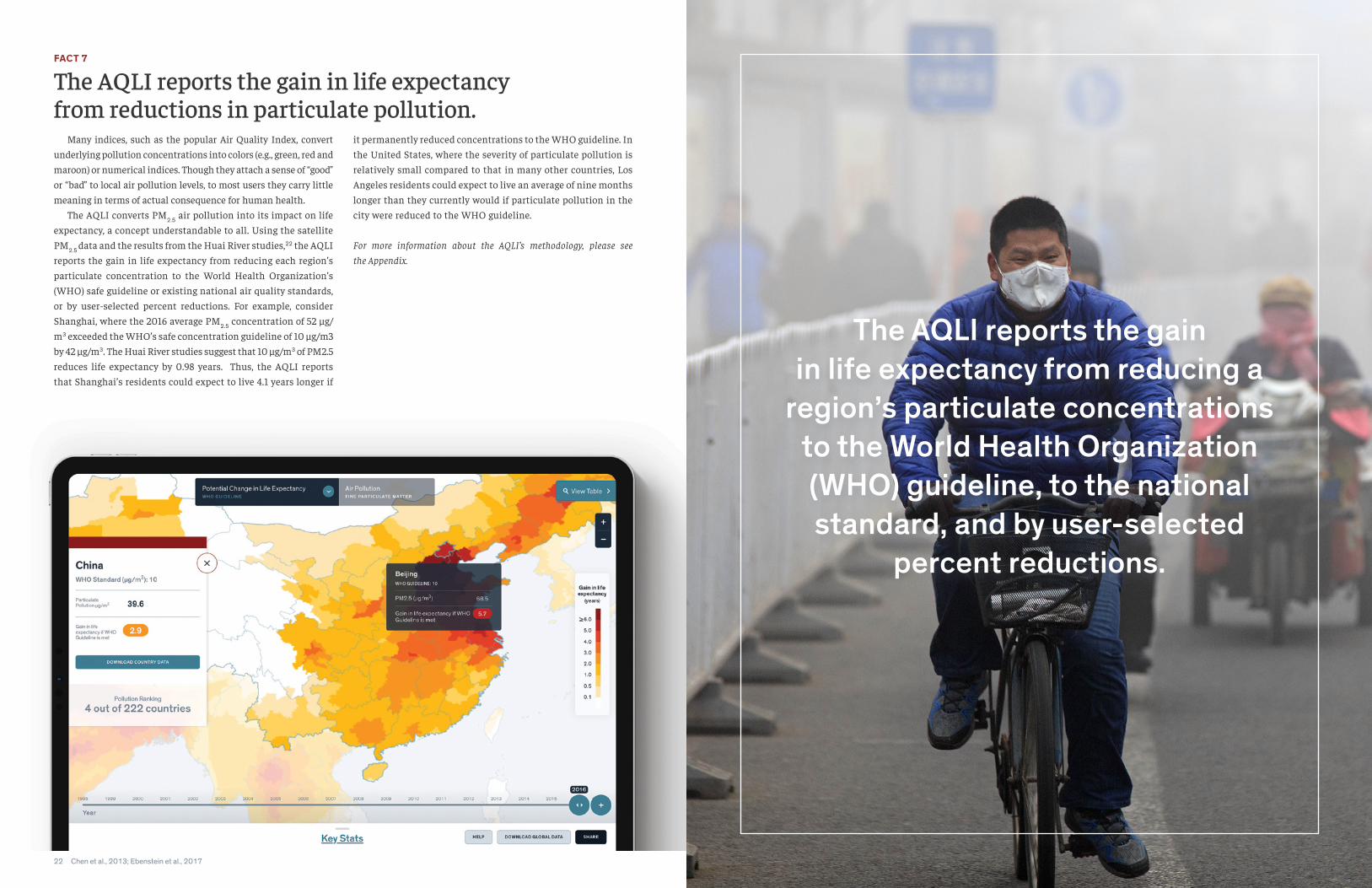
The AQLI reports the gain in life expectancy from reductions in particulate pollution. Many indices, such as the popular Air Quality Index, convert underlying pollution concentrations into colors (e.g., green, red and maroon) or numerical indices. Though they attach a sense of “good” or “bad” to local air pollution levels, to most users they carry little meaning in terms of actual consequence for human health. The AQLI converts PM2.5 air pollution into its impact on life expectancy, a concept understandable to all. Using the satellite PM2.5 data and the results from the Huai River studies,22 the AQLI reports the gain in life expectancy from reducing each region’s particulate concentration to the World Health Organization’s (WHO) safe guideline or existing national air quality standards, or by user-selected percent reductions. For example, consider Shanghai, where the 2016 average PM2.5 concentration of 52 μg/m3 exceeded the WHO’s safe concentration guideline of 10 μg/m3 by 42 μg/m3. The Huai River studies suggest that 10 μg/m3 of PM2.5 reduces life expectancy by 0.98 years. Thus, the AQLI reports that Shanghai’s residents could expect to live 4.1 years longer if

it permanently reduced concentrations to the WHO guideline. In the United States, where the severity of particulate pollution is relatively small compared to that in many other countries, Los Angeles residents could expect to live an average of nine months longer than they currently would if particulate pollution in the city were reduced to the WHO guideline.

For more information about the AQLI’s methodology, please see the Appendix.

The AQLI reports the gain in life expectancy from reducing a

region’s particulate concentrations to the World Health Organization (WHO) guideline, to the national standard, and by user-selected

percent reductions


SECTION IV

The AQLI at WorkThe AQLI reveals that the average person on the planet is losing 1.8 years of life expectancy due to particulate pollution exceeding the WHO guideline—more than devastating communicable diseases like tuberculosis and HIV/AIDS, behavioral killers like cigarette smoking, and even war. Some areas of the world are affected more than others, with the largest losses observed in India, China, and Bangladesh.

FACT 8:

23 Calculations based on GBD 2016. For details, see the Appendix.

Particulate pollution is the greatest external risk to human health. The WHO has set a guideline of 10 µg/m3 as the safe level of long-term average particulate pollution. Relative to what life expectancy would be if all areas complied with this guideline, if current particulate pollution levels persist, today’s global population will lose a total of 12.8 billion years of life directly due to particulate pollution. If the entire planet permanently met the WHO guideline, the average person would live 1.8 years longer, extending life expectancy to 74 years. To put this in perspective, first-hand cigarette smoke leads to a reduction in global average life expectancy of about 1.6 years; alcohol and drugs reduce life expectancy by 11 months; unsafe water and sanitation take off 7 months; and HIV/AIDS, 4 months. Conflict and terrorism take off 22 days. So, the impact of particulate pollution on life expectancy is comparable to that of smoking, twice that of alcohol and drug use, three times that of unsafe water, five times that of HIV/AIDS, and 29 times that of conflict and terrorism.23

What accounts for particulate pollution’s enormous overall impact? The key difference is that residents of polluted areas can do very little to avoid particulate pollution, since everyone breathes the air. In contrast, it is possible to quit smoking and take precautions against diseases. Thus, air pollution affects many more people than any of these other conditions: 75 percent of the global population, or 5.5 billion people, live in areas where PM2.5

exceeds the WHO guideline. So, although other risks such as HIV/AIDS, tuberculosis, or war have a larger impact among the affected, they affect far fewer people. For example, the Global Burden of Disease estimates that those who died from HIV/AIDS in 2016 died prematurely by an average of 51.8 years. However, since the 36 million people affected by the disease is tiny compared to the 5.5 billion people breathing polluted air, the overall impact of air pollution is much greater.

Figure 5 · Average Life Expectancy Lost Per Person

ParticulatePollution

1.8 years1.6 years

11 months

7 months4.5 months 4 months 4 months 3.5 months

22 days

Unsafe Water,Sanitation,

Handwashing

Con�ict andTerrorism

RoadInjuries

Smoking Alcohol and Drug Use

HIV/AIDS Malaria Tuberculosis


FACT 9

24 IEA, 2018

25 BP Energy Outlook 2018 data pack

The average loss in life expectancy due to particulate pollution has increased from 1.0 in 1998 to 1.8 in 2016. Particulate pollution increased between 1998 and 2016 globally, causing a reduction in life expectancy for the average person of about 9 months. Average life expectancy would have been 1.0 years longer in 1998 if air quality met the WHO guideline globally. By 2016, this had increased to 1.8 years due to a 7.8 µg/m3 increase in average particulate pollution concentrations. Developing countries, mostly in Asia and Africa, saw the largest increases in particulate pollution between 1998 and 2016. Over the course of these almost 20 years, industrialization, economic development, and population growth have greatly increased energy demand in these countries. For example, in China, which has experienced breakneck economic growth, coal-generated electricity increased more than five-fold from 1995 to 2015; in India, it increased more than three-fold.24

This greater energy use has enabled economic output and material consumption that have undoubtedly enhanced well-being, but it has also released more particulates into the air. Furthermore, energy demand in non-OECD regions is projected to continue growing,25 so the upward trend in particulate pollution severity is likely to continue without concerted policy actions.

By contrast, North American and many European countries have seen their particulate pollution decrease in the past decades. Though they once suffered from severe particulate pollution, with levels rivaling those in today’s most polluted countries, the offshoring of polluting industries abroad and, crucially, well-implemented air pollution policies have played large roles in attaining clean air for many of these countries. Today, the average American or Briton loses about a month of life due to particulate pollution.

Figure 6 · The average loss in life expectancy due to particulate pollution has increased from 1.0 in 1998 to 1.8 in 2016

World

World PM Increased PM Decreased

China India Indonesia Pakistan Nigeria Bangladesh U.S. Brazil Mexico Germany France U.K.

4 Years

3

2

1

0

2016

1998

This graph shows the loss in life expectancy at 1998 and 2016 PM2.5 levels, relative to the WHO guideline, globally and for the most populous countries that experienced increases and decreases in pollution.

FACT 10

Current particulate pollution concentrations are projected to shorten the lives of 635 million people by at least five years. Developing and industrializing Asian countries are impacted the most by particulate pollution. If in 2016, the WHO PM2.5 guideline were met globally:• 288 million people, all in northern India, would live at least 7

years longer on average. These people represent 23 percent of India’s current population.

• 347 million people in Asia would live 5 to 7 years longer on aver-age. These include 35 percent of Nepal’s population, 16 percent of Bangladeshis, 13 percent of Chinese, 10 percent of Pakistanis, 9 percent of Indians, and 1 percent of Indonesians.

• 937 million people in Asia and Africa would live 3 to 5 years longer on average. These include 76 percent of Bangladeshis, 46 percent of Nepalis, 29 percent of the population of the Republic of Congo, 29 percent of Chinese, 29 percent of Pakistanis, 24 per-cent of Indians, and others in Southeast Asia and Africa.

• An additional 4.1 billion people around the world would live up to 3 years longer, with an average gain of 1.1 years.

In fact, India and China, which make up 36 percent of the world population, account for 73 percent of all years of life lost

due to particulate pollution. On average, people in India would live 4.3 years longer if their country met the WHO guideline. Since life expectancy at birth is currently 69 years in India, this suggests that reducing particulate pollution to the WHO guideline throughout the country would raise the average life expectancy to 73. In comparison, eliminating tuberculosis, a well-known killer in India, would raise the life expectancy to 70. In China, people would live an average of 2.9 years longer if the country met the WHO guideline, increasing Chinese average life expectancy from 76 years to 79. This makes particulate pollution an even bigger killer than cigarette smoking in China, which has high smoking rates. By contrast, the high-income OECD countries, which make up 18 percent of the world’s population, account for less than 3 percent of the health burden of particulate pollution. In the United States, about a third of the population lives in areas not in compliance with the WHO guideline. Those living in the country’s most polluted counties could expect to live up to one year longer if pollution met the WHO guideline.

Figure 7 · Global Distribution of Life Expectancy Lost to Particulate Pollution

2 31 4 5 6 7 8 9 10 11 12

2000 Million

1500

1000

500

0

China

India

Bangladesh

Pakistan

Indonesia

OECD

Rest of the World

People

Years of Life Lost Relative to WHO Guideline


SECTION V

Track Record of Pollution PoliciesLondon was known as “the big smoke” during its period of in-dustrialization. Osaka, Japan, was likewise the “smoke capital.” And, Los Angeles was the “smog capital of the world” as the United States boomed following World War II. Now, these rich, vibrant, and much cleaner cities are evidence that today’s pol-lution does not need to be tomorrow’s fate. But the air did not become cleaner in these countries by accident. Much of it was the result of forceful policies.

FACT 11

26 To extend back to 1970, this analysis is based on monitor data from the U.S. EPA, rather than satellite data that only dates back to 1998. Where they do overlap, this data may differ slightly from the AQLI’s satellite data of PM2.5. For details on how the calculations were done, see aqli.epic.uchicago.edu/policy-impacts/united-states-clean-air-act.

U.S. residents are living 1.5 years longer than in 1970 thanks to reductions in particulate pollution.26

Today, particulate air pollution is not a major problem in most parts of the United States. However, that was not always the case. Following World War II, American industry rebounded from the Great Depression, the population grew as the “baby boom” generation was born, the first highways were built, and modern appliances were popping up in homes throughout the country. With home and industrial energy consumption increasing, and more vehicles on the roads, pollution began to grow. By 1970, the Mobile, Alabama, metropolitan area had particulate pollution concentrations similar to those in Beijing in recent years. Los

Angeles had become known as the smog capital of the world, and other large metropolitan areas faced similar challenges. With pollution becoming part of everyday life for many Americans, political pressure to act began to mount. In 1970, the Clean Air Act established the National Ambient Air Quality Standards (NAAQS), setting maximum allowable concentrations of particulate matter, among other pollutants. It also created emissions standards for pollution sources, leading industrial facilities to install pollution control technologies and automakers to produce cleaner, more fuel-efficient vehicles. Further, it required each state government to devise its own plan for achieving and sustaining compliance with the standards. The Act quickly made an impact on the quality of the air Americans breathed. By 1980, control of industrial emissions had led to a 50 percent decrease in particulate emissions. Today, on

average, Americans are exposed to 60 percent less PM2.5 pollution than they would have been in 1970. With less pollution in the air, citizens are living healthier—and longer—lives. For example, in the former smog capital of Los Angeles, particulate pollution has declined by almost 40 percent since 1970, extending life expectancy for the average Angeleno by a year. Residents of New York have gained more than two years on average, residents of Chicago two years, and residents of Washington, DC have gained almost three years. With 49 million people currently living in these four metropolitan areas, the total

gains in life expectancy add up quickly. The smaller towns and cities, home to industries that for decades prior to 1970 operated with minimal pollution controls, saw some of the greatest improvements. In 1970, residents of Mobile, Alabama could have expected to lose almost 4 years of life due to air pollution relative to a scenario in which they were breathing air that met today’s WHO guideline. Today, pollution in Mobile is down by 84 percent, resulting in effectively no threat to life expectancy versus today’s WHO guideline. About 213 million people currently live in U.S. areas monitored for particulates in 1970 and today. On average, these people can expect to live an additional 1.5 years due to cleaner air alone, for a total gain of about 325 million life-years.

http://aqli.epic.uchicago.edu/policy-impacts/united-states-clean-air-act


FACT 12

27 This Fact Sheet reports pollution data and associated life expectancy results from the AQLI’s own satellite-derived pollution dataset. Thus, they are generally lower than the pollution and life expectancy results in the “Is China Winning its War on Pollution?” report, which are based on the Chinese government’s ground-level pollution monitors. Since China’s War on Pollution is a recent policy initiative, the report uses monitor data to (1) cover an additional year, 2017, when much pollution reduction progress was made, and (2) avoids satellite data’s potential error in measuring pollution trends over a short time span. An additional cause of discrepancies between the data sources is that the AQLI’s pollution data is net of dust, which is a substantial part of what monitors observe – e.g. about 8% in Beijing.

China is winning its “War on Pollution”.27

Public concern about worsening air pollution began rising in the late 1990s. Beginning in 2008, the U.S. embassy in Beijing began publicly posting readings from its own air quality monitor on Twitter and the State Department website, and residents quickly pointed out the conflicts with the city government’s air quality reports. In 2013, concern mounted even further, as some of the highest particulate pollution concentrations China had experienced coincided with the publication of the Chen et al. (2013) Huai River study, which found that high air pollution had cut the lifespans of people in northern China short by about five years compared to those living in the south. The very next year, Premier Li Keqiang declared a “war against pollution.” The National Air Quality Action Plan set aside $270 billion, and the Beijing city government set aside an additional $120 billion, to reduce ambient air pollution. Across all urban areas, the Plan aimed to achieve PM10 reductions of 10 percent in 2017 relative to 2012 levels. The most heavily-polluted areas in the country, including Beijing-Tianjin-Hebei, the Pearl River Delta, and Yangtze River Delta, were given specific targets. The government’s strategies for achieving these goals included building pollution reduction into local officials’ incentives so promotions depended on both environmental audits and economic performance; prohibiting new coal-fired plants in some regions and requiring existing coal plants to reduce emissions or be replaced with natural gas; increasing renewable energy generation; reducing iron and steel making capacity in industry; restricting the number

of cars on the road in large cities; and increasing transparency and better enforcing emissions standards. Thanks to these actions, between 2013 and 2016, particulate pollution exposure declined by an average of 12 percent across the Chinese population. If that reduction is sustained, it would equate to a gain in life expectancy of 0.5 years. Tianjin, one of China’s three most polluted cities in 2013, saw a 14 percent reduction in particulate pollution, translating to a gain of 1.2 years of life expectancy for its 13 million residents, if sustained. In Henan, the province that saw the largest pollution reduction, residents are exposed to 20 percent less particulate pollution than in 2013, equating to a 1.3 year gain in life expectancy. To put China’s success in context, the pollution reduction in China from 2013-2016 is greater than that seen in the United States from 1998-2016. Satellite-derived particulate pollution data is not yet available for 2017, the last year of the National Air Quality Action Plan’s timespan. However, the Ministry of Environmental Protection and local officials took aggressive measures in that year to ensure that targets would be met in the key regions of Beijing-Tianjin-Hebei, the Pearl River Delta, and the Yangtze River Delta. Though these aggressive actions have come with some unintended consequences—for example, some homes and businesses had no heat in the winter of 2017-2018 because their coal boilers were removed before replacements were installed—these steps would have further reduced particulate pollution to below 2016 levels, even as they underscored the need for longer-term solutions to make the reductions permanent.

China’s particulate pollution declined by 12 percent in the span of three years, resulting in a gain

in life expectancy of 0 5 years


AppendixDATA AND METHODOLOGY The AQLI estimates the relationship between air pollution and life expectancy, allowing users to view the gain in life expectancy they could experience if their community met World Health Organization (WHO) guidelines, national standards or some other standard. It does so by leveraging results from a pair of studies set in China. The results of the studies are combined with detailed global population and PM2.5 data to estimate the impact of particulate matter on life expectancy across the globe.

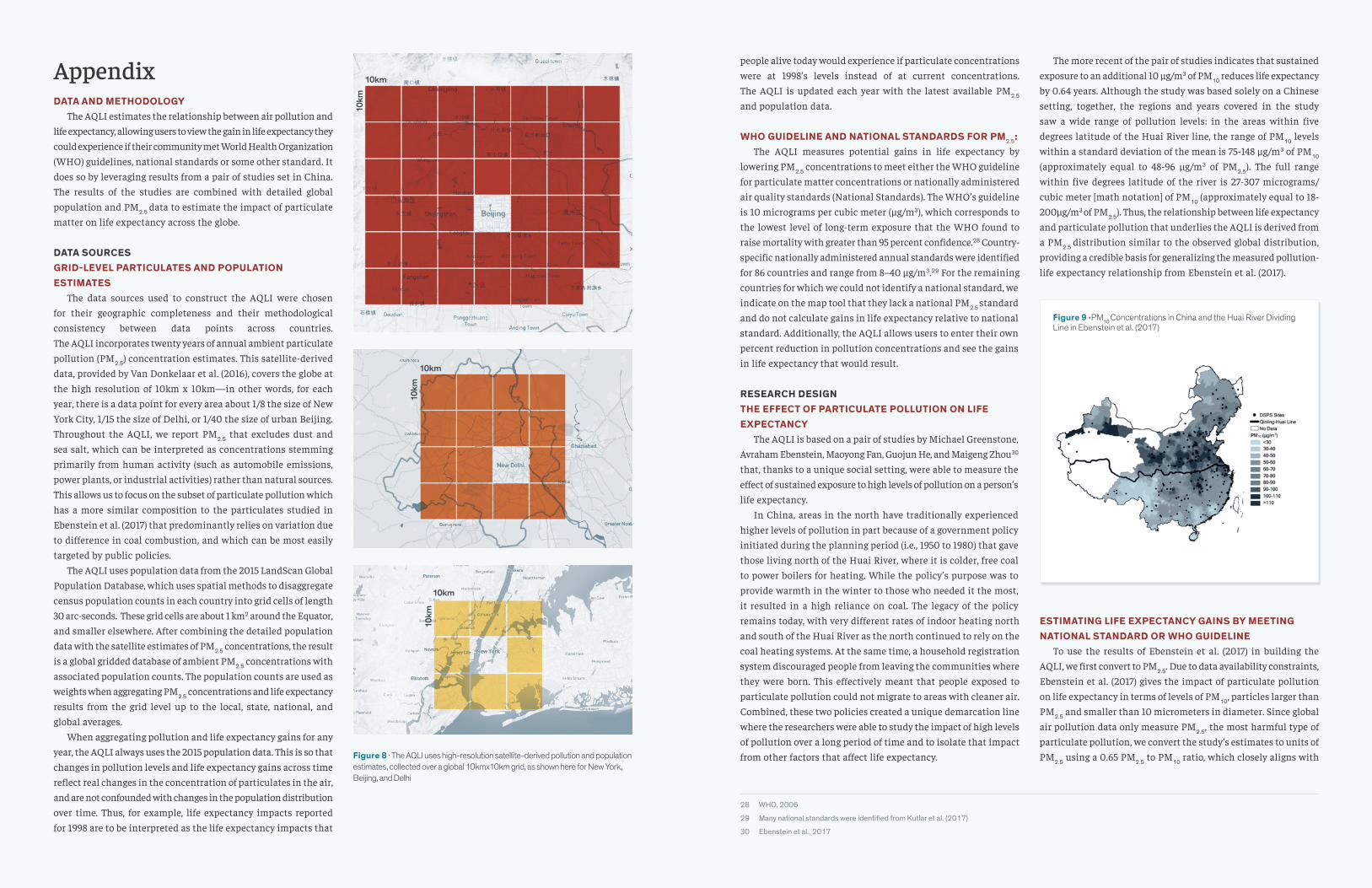
DATA SOURCESGRID-LEVEL PARTICULATES AND POPULATION ESTIMATES The data sources used to construct the AQLI were chosen for their geographic completeness and their methodological consistency between data points across countries. The AQLI incorporates twenty years of annual ambient particulate pollution (PM2.5) concentration estimates. This satellite-derived data, provided by Van Donkelaar et al. (2016), covers the globe at the high resolution of 10km x 10km—in other words, for each year, there is a data point for every area about 1/8 the size of New York City, 1/15 the size of Delhi, or 1/40 the size of urban Beijing. Throughout the AQLI, we report PM2.5 that excludes dust and sea salt, which can be interpreted as concentrations stemming primarily from human activity (such as automobile emissions, power plants, or industrial activities) rather than natural sources. This allows us to focus on the subset of particulate pollution which has a more similar composition to the particulates studied in Ebenstein et al. (2017) that predominantly relies on variation due to difference in coal combustion, and which can be most easily targeted by public policies. The AQLI uses population data from the 2015 LandScan Global

Population Database, which uses spatial methods to disaggregate census population counts in each country into grid cells of length 30 arc-seconds. These grid cells are about 1 km2 around the Equator, and smaller elsewhere. After combining the detailed population data with the satellite estimates of PM2.5 concentrations, the result is a global gridded database of ambient PM2.5 concentrations with associated population counts. The population counts are used as weights when aggregating PM2.5 concentrations and life expectancy results from the grid level up to the local, state, national, and global averages. When aggregating pollution and life expectancy gains for any year, the AQLI always uses the 2015 population data. This is so that changes in pollution levels and life expectancy gains across time reflect real changes in the concentration of particulates in the air, and are not confounded with changes in the population distribution over time. Thus, for example, life expectancy impacts reported for 1998 are to be interpreted as the life expectancy impacts that

Figure 8 · The AQLI uses high-resolution satellite-derived pollution and population estimates, collected over a global 10kmx10km grid, as shown here for New York, Beijing, and Delhi

people alive today would experience if particulate concentrations were at 1998’s levels instead of at current concentrations. The AQLI is updated each year with the latest available PM2.5

and population data.

WHO GUIDELINE AND NATIONAL STANDARDS FOR PM2.5: The AQLI measures potential gains in life expectancy by lowering PM2.5 concentrations to meet either the WHO guideline for particulate matter concentrations or nationally administered air quality standards (National Standards). The WHO’s guideline is 10 micrograms per cubic meter (μg/m3), which corresponds to the lowest level of long-term exposure that the WHO found to raise mortality with greater than 95 percent confidence.28 Country-specific nationally administered annual standards were identified for 86 countries and range from 8–40 μg/m3.29 For the remaining countries for which we could not identify a national standard, we indicate on the map tool that they lack a national PM2.5 standard and do not calculate gains in life expectancy relative to national standard. Additionally, the AQLI allows users to enter their own percent reduction in pollution concentrations and see the gains in life expectancy that would result.

RESEARCH DESIGNTHE EFFECT OF PARTICULATE POLLUTION ON LIFE EXPECTANCY The AQLI is based on a pair of studies by Michael Greenstone, Avraham Ebenstein, Maoyong Fan, Guojun He, and Maigeng Zhou30 that, thanks to a unique social setting, were able to measure the effect of sustained exposure to high levels of pollution on a person’s life expectancy. In China, areas in the north have traditionally experienced higher levels of pollution in part because of a government policy initiated during the planning period (i.e., 1950 to 1980) that gave those living north of the Huai River, where it is colder, free coal to power boilers for heating. While the policy’s purpose was to provide warmth in the winter to those who needed it the most, it resulted in a high reliance on coal. The legacy of the policy remains today, with very different rates of indoor heating north and south of the Huai River as the north continued to rely on the coal heating systems. At the same time, a household registration system discouraged people from leaving the communities where they were born. This effectively meant that people exposed to particulate pollution could not migrate to areas with cleaner air. Combined, these two policies created a unique demarcation line where the researchers were able to study the impact of high levels of pollution over a long period of time and to isolate that impact from other factors that affect life expectancy.

28 WHO, 2006

29 Many national standards were identified from Kutlar et al. (2017)

30 Ebenstein et al., 2017

The more recent of the pair of studies indicates that sustained exposure to an additional 10 μg/m3 of PM10 reduces life expectancy by 0.64 years. Although the study was based solely on a Chinese setting, together, the regions and years covered in the study saw a wide range of pollution levels: in the areas within five degrees latitude of the Huai River line, the range of PM10 levels within a standard deviation of the mean is 75-148 µg/m3 of PM10 (approximately equal to 48-96 µg/m3 of PM2.5). The full range within five degrees latitude of the river is 27-307 micrograms/cubic meter [math notation] of PM10 (approximately equal to 18-200µg/m3 of PM2.5). Thus, the relationship between life expectancy and particulate pollution that underlies the AQLI is derived from a PM2.5 distribution similar to the observed global distribution, providing a credible basis for generalizing the measured pollution-life expectancy relationship from Ebenstein et al. (2017).

ESTIMATING LIFE EXPECTANCY GAINS BY MEETING NATIONAL STANDARD OR WHO GUIDELINE To use the results of Ebenstein et al. (2017) in building the AQLI, we first convert to PM2.5. Due to data availability constraints, Ebenstein et al. (2017) gives the impact of particulate pollution on life expectancy in terms of levels of PM10, particles larger than PM2.5 and smaller than 10 micrometers in diameter. Since global air pollution data only measure PM2.5, the most harmful type of particulate pollution, we convert the study’s estimates to units of PM2.5 using a 0.65 PM2.5 to PM10 ratio, which closely aligns with

Figure 9 ·PM10 Concentrations in China and the Huai River Dividing Line in Ebenstein et al. (2017)

10km

10km

10km

10km

10km

10km


conditions in China during the time period of the study.31 This translates to:

In other words, life expectancy is reduced 0.98 years per 10 μg/m3 of sustained exposure to PM2.5. Following the epidemiology literature,32 the AQLI assumes a linear relationship between long-term exposure to PM2.5 and life expectancy throughout the observed PM2.5 distribution. Though it is possible that the pollution-life expectancy relationship is nonlinear over certain ranges of PM2.5 concentrations and/or that there is a threshold below which PM2.5 has no effect, we are unaware of credible empirical evidence that would cause a rejection of the linearity assumption. Therefore, to estimate the potential gain in life expectancy within each grid-cell, the AQLI increases the loss in life expectancy by 0.98 years for every 10 μg/m3 of additional long-term exposure above the reference standard (either the WHO guideline or national standard, or a user entered standard). For both pollution concentrations and loss in life expectancy, the AQLI aggregates grid-cell-level estimates to national and sub-national administrative boundaries. Aggregations are population-weighted. For example, in 2016, the annual average PM2.5 level in Beijing was 68.5 μg/m3, and the level in Guangzhou was 34.3 μg/m3. When calculating China’s national 2016 annual average PM2.5 level, Beijing’s PM2.5 level is given about 50 percent more weight than Guangzhou’s, because Beijing’s population is about 1.5 times that of Guangzhou. Thus, China’s national average PM2.5 level of 39.6 μg/m3 means that on average, each person in China was exposed to an annual average PM2.5 level of 39.6 μg/m3 in 2016. These aggregated values are what is shown in the map tool.

A NOTE ON THE AQLI’S POLLUTION DATA Users may find that the AQLI’s pollution data differs from other databases, such as those used by the WHO and the Global Burden of Disease (GBD). One difference is in raw data. The AQLI uses annual data for each year from 1998-2016 instead of three-year rolling averages. However, compared to the WHO’s data, the available annual data uses a less sophisticated method of calibrating satellite and ground measurements. These result in the AQLI’s data source generally reporting lower pollution levels

31 The ratio of 0.65 is based on a careful review of studies that report historical PM2.5-to-PM10 ratios in China during a similar timeframe as Ebenstein (2017). Two nationally representative studies are of particularly interest. Wang et al. (2015) measures PM2.5-to-PM10 ratios at 24 monitoring stations across the country between 2006 and 2014 and reports total averages by station/city. A back of the envelope population weighted-average calculation using these averages indicates a PM2.5-to-PM10 ratio of 0.73. Importantly, the list of cities in this study does not include some major metropolitan areas (e.g. Beijing), although many surrounding areas are included. Zhou et al. (2015) compiles a comprehensive nationwide database of all published literature (128 articles) which studied PM2.5 and PM10 mass concentrations from 1988 – 2010 and finds a PM2.5-to-PM10 ratio of 0.65 based on 589 pairs of data covering 57 cities and regions. Finally, we also considered the mass ratio PM2.5/PM10 of 0.66 used by the World Health Organization for China in its ambient pollution database. Given the comprehensiveness of Zhou et al. (2015) and how close its findings are to the WHO value (0.65 versus 0.66), we use 0.65 as the baseline PM2.5-to-PM10 ratio for the AQLI.

32 See, for example, Global Burden of Disease (2016).

33 WHO, 2018

than the WHO. In addition, the AQLI removes dust and sea salt, while the WHO and the GBD do not, leading to more differences. For example, removing dust and sea salt reduces reported PM2.5

in Delhi by about 15 percent, and by about 8 percent for Beijing. In North Africa and the Middle East, Sub-Saharan Africa, and northwestern China, they are a significant portion of total PM2.5

concentrations, leading to even larger differences. Since the AQLI’s satellite-derived PM2.5 data begins in 1998 and ends before the present year, the Policy Impacts pages also make use of monitor-based pollution data to measure the impact of policies enacted before 1998 and/or that continue to be associated with significant changes in pollution levels today. Users reading the Policy Impact pages or comparing AQLI data to their local air quality monitors’ annual averages may note discrepancies between monitor and satellite-derived measurements. Aside from differences due to the AQLI’s exclusion of dust and sea salt, discrepancies may also arise from limitations of satellites. For example, satellites can measure air pollution only on relatively cloud-free days; in many areas, pollution is most severe in winter, when there are few such days. In such cases, monitor measurements are likely to be more accurate. However, monitor measurements are unavailable in many countries, and measurement technologies and methodologies are inconsistent from place to place, rendering them difficult to compare. Since satellite-derived pollution data are available for around the world and based on a single methodology, it is the primary data of the AQLI.

COMPARISONS WITH OTHER MORTALITY CAUSES AND RISKS IN FACT 8 Based on the AQLI’s results, if 2016 levels of ambient particulate pollution are sustained around the world, the life expectancy of everyone alive today would be on average 1.8 years lower than if particulate concentrations everywhere complied with the WHO guideline. In Fact 8, we compare this finding with the life expectancy impacts of other causes and risks of premature death. We do so using life tables, the same epidemiological approach that the Huai River studies used to calculate the relationship between particulate pollution and life expectancy. A summary of this approach is as follows. From the WHO,33 we obtain a life table of 2016 mortality data such as probability of death and life expectancy remaining for each sex and age interval 0-1, 1-4, 5-9, …, 80-84, and 85+. We call these the “baseline” data. From the Global Burden of Disease 2016 (GBD), for a variety of

causes and risks of mortality (e.g. smoking, malaria), we obtain the rates of death in 2016 due to that cause or risk within each sex and age interval 0-1, 1-4, 5-9, …, 75-79, and 80+. For both of these data sets, we aggregate the highest age intervals into a single 80+ interval for consistency. Now, using the baseline life table and following the procedure first outlined by Greenwood (1922) and Chiang (1984), we calculate average life expectancy for a male and a female born in 2016, assuming that mortality risks in each age interval remain constant into the future. Using the 2016 sex ratio at birth34, we take a weighted average to aggregate the life expectancies by sex into a single average baseline life expectancy. This number accounts for the life expectancy impacts of all mortality causes and risks, based on their actual burdens in 2016.

34 U.N. Population Division, 2017

To calculate what life expectancy at birth in 2016 would hypothetically have been if a particular condition (e.g. smoking or malaria) did not exist, we subtract rates of death due to that condition from the life table baseline rates, then follow the same procedure as above to obtain the counterfactual average life expectancy at birth. The difference between the baseline life expectancy and this counterfactual life expectancy is the life expectancy impact of that condition, which we compare to the AQLI’s result of 1.8 years for particulate pollution.

The data and code that produced these calculations can be found at aqli.epic.uchicago.edu/about/methodology

http://aqli.epic.uchicago.edu/about/methodology/


CountryPM2.5 (µ g/m3) Concentration

National Standard

Life Years Saved:

National Standard

Life Years Saved:

WHO Guideline Country

PM2.5 (µ g/m3) Concentration

National Standard

Life Years Saved:

National Standard

Life Years Saved:

WHO Guideline

Afghanistan 14 10 0.5 0.5

Akrotiri and Dhekelia 9 n/a 0 0

Aland 6 n/a 0 0

Albania 10 15 0 0.1

Algeria 8 n/a 0 0

American Samoa 0 n/a 0 0

Andorra 4 25 0 0

Angola 18 n/a 0.1 0.8

Antigua and Barbuda 0 n/a 0 0

Argentina 10 15 0.1 0.2

Armenia 18 n/a 0 0.8

Australia 3 8 0 0

Austria 13 25 0 0.4

Azerbaijan 18 n/a 0 0.8

Bahamas 1 n/a 0 0

Bahrain 19 n/a 0 0.9

Bangladesh 53 15 3.8 4.2

Barbados 1 n/a 0 0

Belarus 16 15 0.1 0.5

Belgium 14 25 0 0.4

Belize 2 n/a 0 0

Benin 13 n/a 0 0.4

Bermuda 1 30 0 0

Bhutan 23 n/a 0.5 1.3

Bolivia 10 10 0.2 0.2

Bonaire, Sint Eustatius and Saba 1 n/a 0 0

Bosnia and Herzegovina 12 25 0 0.3

Botswana 16 n/a 0 0.6

Brazil 8 n/a 0 0.2

British Virgin Islands 1 n/a 0 0

Brunei 8 n/a 0 0

Bulgaria 13 25 0 0.3

Burkina Faso 5 n/a 0 0

Burundi 21 n/a 0.1 1.1

Cambodia 17 n/a 0 0.7

Cameroon 15 10 0.7 0.7

Canada 6 10 0 0

Cape Verde 1 n/a 0 0

Cayman Islands 2 n/a 0 0

Central African Republic 17 n/a 0 0.7

Chad 6 n/a 0 0

Chile 18 20 0.3 0.9

China 39 35 1 2.9

Colombia 8 25 0 0.1

Comoros 2 n/a 0 0

Costa Rica 3 n/a 0 0

Cote d'Ivoire 11 n/a 0 0.2

Croatia 14 25 0 0.4

Cuba 3 n/a 0 0

Cyprus 8 25 0 0

Czech Republic 17 25 0 0.7

Democratic Republic of the Congo 28 n/a 0.8 1.8

Denmark 10 25 0 0

Djibouti 8 n/a 0 0

Dominica 1 n/a 0 0

Dominican Republic 3 15 0 0

Ecuador 9 15 0 0

Egypt 10 n/a 0 0.1

El Salvador 8 15 0 0

Equatorial Guinea 17 n/a 0 0.7

Eritrea 7 n/a 0 0

Estonia 8 25 0 0

Ethiopia 16 n/a 0 0.7

Faroe Islands 1 n/a 0 0

Fiji 0 n/a 0 0

Finland 7 25 0 0

France 10 25 0 0.1

French Guiana 1 n/a 0 0

French Polynesia 0 n/a 0 0

French Southern Territories 3 n/a 0 0

Gabon 21 n/a 0.1 1

Gambia 3 n/a 0 0

Georgia 13 n/a 0 0.3

Germany 13 25 0 0.3

Ghana 15 n/a 0 0.5

Greece 10 25 0 0.1

Greenland 1 n/a 0 0

Grenada 1 n/a 0 0

Guadeloupe 1 25 0 0

Guam 0 12 0 0

Guatemala 8 10 0 0

Guernsey 10 n/a 0 0

Guinea 6 n/a 0 0

Guinea-Bissau 4 n/a 0 0

Guyana 1 n/a 0 0

Haiti 4 n/a 0 0

Honduras 5 n/a 0 0

Hungary 19 25 0 0.9

Iceland 2 n/a 0 0

India 54 40 1.8 4.3

Indonesia 22 n/a 0.5 1.2

Iran 11 10 0.2 0.2

Iraq 9 n/a 0 0.1

Ireland 4 25 0 0

Isle of Man 7 n/a 0 0

Israel 9 25 0 0

Italy 14 25 0 0.5

Jamaica 2 15 0 0

Japan 12 15 0 0.2

Jersey 9 n/a 0 0

Jordan 7 15 0 0

Kazakhstan 13 n/a 0 0.4

Kenya 10 35 0 0.2

Kosovo 12 n/a 0 0.2

Kuwait 14 15 0 0.4

Kyrgyzstan 14 n/a 0 0.4

Laos 30 n/a 1 2

Latvia 11 25 0 0.1

Lebanon 8 n/a 0 0

Lesotho 14 n/a 0 0.4

Liberia 8 n/a 0 0

Libya 5 n/a 0 0

Liechtenstein 7 n/a 0 0

Lithuania 14 25 0 0.4

Luxembourg 10 25 0 0

Macedonia 12 n/a 0 0.2

Madagascar 4 n/a 0 0

Malawi 11 8 0.3 0.1

Malaysia 17 35 0 0.8

Mali 3 n/a 0 0

Martinique 1 25 0 0

Mauritania 2 n/a 0 0

Mauritius 0 n/a 0 0

Mayotte 2 25 0 0

Mexico 12 15 0.1 0.3

Micronesia 0 n/a 0 0

Moldova 17 n/a 0 0.7

Mongolia 11 25 0 0.3

Montenegro 10 20 0 0.1

Montserrat 1 n/a 0 0

Morocco 9 n/a 0 0.1

Mozambique 8 n/a 0 0

Myanmar 23 n/a 0.2 1.2

Namibia 10 n/a 0 0.2

Nauru 0 n/a 0 0

Nepal 55 n/a 3.3 4.4

Netherlands 13 25 0 0.3

New Caledonia 0 25 0 0

New Zealand 1 n/a 0 0

Nicaragua 3 n/a 0 0

Niger 5 n/a 0 0

Nigeria 18 n/a 0.3 0.8

North Korea 22 n/a 0.2 1.1

Northern Cyprus 9 n/a 0 0

Northern Mariana Islands 1 n/a 0 0

Norway 4 15 0 0

Oman 10 n/a 0 0.1

Pakistan 37 15 2.2 2.7

Palau 1 n/a 0 0

Palestina 9 n/a 0 0

Panama 2 n/a 0 0

Papua New Guinea 2 n/a 0 0

Paraguay 10 15 0 0.1

Peru 17 15 0.7 0.9

Philippines 7 25 0 0.1

Poland 21 25 0 1

Portugal 5 25 0 0

Puerto Rico 1 15 0 0

Qatar 19 n/a 0 0.9

Republic of Congo 34 n/a 1.2 2.3

Reunion 0 n/a 0 0

Romania 16 25 0 0.6

Russia 15 25 0 0.5

Rwanda 24 n/a 0.3 1.4

Saint Helena 1 n/a 0 0

Saint Kitts and Nevis 1 n/a 0 0

Saint Lucia 1 n/a 0 0

Saint Pierre and Miquelon 1 n/a 0 0


National Standard

Life Years Saved:

National Standard

Life Years Saved:



National Standard

Life Years Saved:

National Standard

Life Years Saved:

WHO Guideline

Saint Vincent and the Grenadines 1 n/a 0 0

Samoa 0 n/a 0 0

San Marino 13 n/a 0 0.3

Sao Tome and Principe 11 n/a 0 0.1

Saudi Arabia 12 15 0.1 0.2

Senegal 3 n/a 0 0

Serbia 15 25 0 0.5

Seychelles 1 n/a 0 0

Sierra Leone 7 n/a 0 0

Singapore 25 12 1.3 1.5

Slovakia 20 25 0 1

Slovenia 13 n/a 0 0.3

Solomon Islands 1 n/a 0 0

Somalia 4 n/a 0 0

South Africa 20 20 0.6 1.1

South Korea 24 25 0.1 1.4

South Sudan 11 n/a 0 0.2

Spain 7 25 0 0

Sri Lanka 1 25 0 0

Sudan 6 n/a 0 0

Suriname 1 n/a 0 0

Swaziland 14 n/a 0 0.4

Sweden 7 25 0 0

Switzerland 10 n/a 0 0

Syria 11 n/a 0 0.2

Taiwan 14 15 0.2 0.5

Tajikistan 29 n/a 0.8 1.9

Tanzania 11 n/a 0 0.2

Thailand 31 25 0.8 2.1

Timor-Leste 4 n/a 0 0

Togo 14 n/a 0 0.5

Tokelau 1 n/a 0 0

Tonga 0 n/a 0 0

Trinidad and Tobago 1 15 0 0

Tunisia 5 n/a 0 0

Turkey 12 n/a 0 0.2

Turkmenistan 12 n/a 0 0.2

Turks and Caicos Islands 1 25 0 0

Tuvalu 0 n/a 0 0

Uganda 20 n/a 0.2 1

Ukraine 17 n/a 0 0.7

United Arab Emirates 18 n/a 0 0.8

United Kingdom 10 25 0 0.1

United States 9 12 0 0.1

United States Minor Outlying 0 n/a 0 0

Uruguay 6 n/a 0 0

Uzbekistan 24 n/a 0.4 1.3

Vanuatu 1 n/a 0 0

Venezuela 3 n/a 0 0

Vietnam 20 25 0.3 1

Virgin Islands, U S 1 12 0 0

Wallis and Futuna 0 n/a 0 0

Western Sahara 1 n/a 0 0

Yemen 7 n/a 0 0

Zambia 16 n/a 0 0.6

Zimbabwe 12 n/a 0 0.2


National Standard

Life Years Saved:

National Standard

Life Years Saved:



National Standard

Life Years Saved:

National Standard

Life Years Saved:

WHO Guideline


ReferencesBell, M.L. and Davis, D.L. (2001). Reassessment of the lethal London Fog of 1952: Novel indicators of acute and chronic consequences of acute exposure to air pollution. Environmental Health Perspectives, 109: 389-394.

Biondo, S.J. and Marten, J.C. (1977). A history of flue gas desulfurization systems since 1850. Journal of the Air Pollution Control Association, 27(10), 948-961.

BP Energy Outlook. (2018). Data pack [Data file]. Retrieved from https://www.bp.com/en/global/corporate/energy-economics/energy-outlook.html

BP Statistical Review of World Energy. (2012). Available from https://www.bp.com/statisticalreview

Bright, E.A., Rose, A.N., and Urban, M.L. (2016). LandScan 2015 [Data file]. Oak Ridge National Laboratory. Retrieved from https://landscan.ornl.gov/

Chay, K.Y. & Dobkin, C. (2003). The Clean Air Act of 1970 and adult mortality. Journal of Risk and Uncertainty, 27(3): 279-300

Chay, K. Y., & Greenstone, M. (2003). Air quality, infant mortality, and the Clean Air Act of 1970. National Bureau of Economic Research, Working Paper 10053.

Chay, K. Y., & Greenstone, M. (2003). The impact of air pollution on infant mortality: evidence from geographic variation in pollution shocks induced by a recession. The quarterly journal of economics, 118(3), 1121-1167.

Chen, Y., Ebenstein, A., Greenstone, M., & Li, H. (2013). Evidence on the impact of sustained exposure to air pollution on life expectancy from China’s Huai River policy. Proceedings of the National Academy of Sciences, 110(32), 12936-12941.

Chiang, C.L. (1984). The life table and its applications. Malabar, Florida: R.E. Krieger Publishing.

Davis, D. (2002). When Smoke Ran Like Water. New York: Basic Books.

Dockery, D. W., Pope, C. A., Xu, X., Spengler, J. D., Ware, J. H., Fay, M. E., ... & Speizer, F. E. (1993). An association between air pollution and mortality in six US cities. New England journal of medicine, 329(24), 1753-1759.

Dominici, F., Greenstone, M., & Sunstein, C. R. (2014). Particulate matter matters. Science, 344(6181), 257-259.

Ebenstein, A., Fan, M., Greenstone, M., He, G., & Zhou, M. (2017). New evidence on the impact of sustained exposure to air pollution on life expectancy from China’s Huai River Policy. Proceedings of the National Academy of Sciences, 114(39), 10384-10389.

Energy Policy Institute at the University of Chicago. (2018). Levelized Cost of Electricity, India. Mimeo.

Gibbens, S. (2018). Air pollution robs us of our smarts and our lungs. National Geographic. Retrieved from https://www.nationalgeographic.com/environment/2018/09/news-air-quality-brain-cognitive-function/?user.testname=none

Global Burden of Disease. (2016). Retrieved from http://ghdx.healthdata.org/gbd-2016

Greenstone, M. (2015, Sept 23). Overview on methodology for clean air study. The New York Times. Retrieved from https://www.nytimes.com/2015/09/25/upshot/notes-on-methodology.html?module=inline

Greenwood, M. (1922). Discussion on the Value of Life-Tables in Statistical Research. Journal of the Royal Statistical Society, 85(4), 537-560.

Guttikunda, S.K and Jawahar, P. (2014). Atmospheric emissions and pollution from the coal-fired thermal power plants in India. Atmospheric Environment, 92, 449-460.

Iadecola, C. (2013). The pathobiology of vascular dementia. Neuron, 80(4), 844-66.

International Energy Agency. (2018). Electricity generation by fuel, India 1990-2016 [Data file]. Retrieved from https://www.iea.org/statistics

Karagulian, F., Belis, C.A., Dora, C.F., Prüss-Ustün, A.M., Bonjour, S., Adair-Rohani, H., Amann, M. (2015). Contributions to cities’ ambient particulate matter (PM): A systematic review of local source contributions at global level. Atmospheric Environment, 120(2015), 475-483.

Katsouyanni, K., Touloumi, G., Spix, C., Schwartz, J., Balducci, F., Medina, S., …, Anderson, H.R. (1997). Short term effects of ambient sulphur dioxide and particulate matter on mortality in 12 European cities: results from time series data from the APHEA project.

BMJ, 314(7095), 1658.

Kutlar, J.M, Eeftens, M., Gintowt, E., Kappeler, R., Kunzli, N. (2017). Time to Harmonize National Ambient Air Quality Standards. International Journal of Public Health 62(4), 453–462.

Ling, S. H., and van Eeden, S. F. (2009). Particulate matter air pollution exposure: role in the development and exacerbation of chronic obstructive pulmonary disease. International journal of chronic obstructive pulmonary disease, 4, 233-43.

National Research Council. (2010). Global Sources of Local Pollution: An Assessment of Long-Range Transport of Key Air Pollutants to and from the United States. Washington, DC: The National Academies Press.

Philip, S., Martin, R.V., van Donkelaar, A., Lo, J.W., Wang, Y., Chen, D., …, Macdonald, D.J. (2014). Global chemical composition of ambient fine particulate matter for exposure assessment. Environmental Science & Technology, 48(22), 13060-13068.

Pope III, C. A., Ezzati, M., & Dockery, D. W. (2009). Fine-particulate air pollution and life expectancy in the United States. New England Journal of Medicine, 360(4), 376-386.

U.N. Population Division. (2017). Sex Ratio at Birth (SRB) [Data file]. Retrieved from https://population.un.org/wpp/Download/Standard/Fertility/

U.S. Department of Energy. Ultra-low sulfur diesel. Retrieved from https://www.fueleconomy.gov/feg/lowsulfurdiesel.shtml

U.S. Energy Information Administration. (2017a). Average Costs of Existing Flue Gas Desulfurization Units. Retrieved from https://www.eia.gov/electricity/annual/html/epa_09_04.html

U.S. Energy Information Administration. (2017b). Quantity and net summer capacity of operable environmental equipment, 2007-2017. Retrieved from https://www.eia.gov/electricity/annual/html/epa_09_02.html

U.S. Energy Information Administration. (2017c). Existing Capacity by Energy Source, 2017 (Megawatts). Retrieved from https://www.eia.gov/electricity/annual/html/epa_04_03.html

U.S. Energy Information Administration. (2018). Weekly retail gasoline and diesel prices [Data file]. Retrieved from https://www.eia.gov/dnav/pet/pet_pri_gnd_dcus_nus_w.htm

U.S. Environmental Protection Agency. Diesel fuel standards and rulemakings. Retrieved from https://www.epa.gov/diesel-fuel-standards/diesel-fuel-standards-and-rulemakings

Van Donkelaar, A., Martin, R. V., Brauer, M., Hsu, N. C., Kahn, R. A., Levy, R. C., ... & Winker, D. M. (2016). Global estimates of fine particulate matter using a combined geophysical-statistical method with information from satellites, models, and monitors. Environmental science & technology, 50(7), 3762-3772.

Wang Y.Q., Zhang, X.Y., Sun, J.Y., Zhang, X.C., Che, H.Z., and Li, Y. (2015) Spatial and temporal variations of the concentration of PM10, PM2.5 and PM1 in China. Atmospheric Chemistry and Physics, 15:13585-13598.

Wilson, W.E. and Suh, H. H. (1997). Fine particles and coarse particles: Concentration relationships relevant to epidemiological studies. Journal of the Air & Waste Management Association, 47(12), 1238-1249.

World Health Organization. (2006) WHO Air quality guidelines for particulate matter, ozone, nitrogen dioxide and sulfur dioxide. Available at: http://apps.who.int/iris/bitstream/handle/10665/69477/WHO_SDE_PHE_OEH_06.02_eng.pdf

World Health Organization. (2016). WHO Global Urban Ambient Air Pollution Database (update 2016). Available online at: http://www.who.int/phe/health_topics/outdoorair/databases/cities/en/

World Health Organization. (2018). Life tables by WHO region: Global [Data file]. Available at http://apps.who.int/gho/data/view.main.LIFEREGIONGLOBAL?lang=en

Xing, Y. F., Xu, Y. H., Shi, M. H., & Lian, Y. X. (2016). The impact of PM2.5 on the human respiratory system. Journal of thoracic disease, 8(1), E69-74.

Zhou, X., Cao, Z., Ma, Y., Wang, L., Wu, R., and Wang, W. (2015) Concentrations, correlations and chemical species of PM2.5/PM10 based on published data in China: Potential implications for the revised particulate standard. Chemosphere, 144(2016): 518-526.

DESIGNED BY CONSTRUCTIVE

About the Authors

Michael Greenstone

Michael Greenstone is the Milton Friedman Professor in Economics, the College, and the Harris School, as well as the Director of the Becker Friedman Institute and the interdisciplinary Energy Policy Institute at the University of Chicago. Greenstone’s research, which has influenced policy globally, is largely focused on uncovering the benefits and costs of environmental quality and society’s energy choices. As the Chief Economist for President Obama’s Council of Economic Advisers, he co-led the development of the United States Government’s social cost of carbon. Additionally, he has been researching the impacts of particulate pollution on human well-being for more than two decades, including work that plausibly quantified the causal relationship between long-term human exposure to particulate pollution and life expectancy. This work is the basis of the Air Quality Life Index.

Qing (Claire) Fan

Qing (Claire) Fan is a Pre-Doctoral Fellow with the Energy Policy Institute at the University of Chicago (EPIC), where she works for Director Michael Greenstone on a variety of energy and environmental economics projects. She earned her bachelor’s in mathematics with a minor in economics in 2018 from Pomona College in California. While at Pomona, Claire conducted a field study on attitudes toward sustainable agriculture in farming communities in Punjab, India, and worked on research in applied mathematics and on the economics of social enterprise. Claire is interested in the intersection of environmental and development economics, including the social impacts of climate change, and food and agriculture.

AIR QUALITY LIFE INDEX

The AQLI is a pollution index that translates particulate air pollution into perhaps the most important metric that exists: its impact on life expectancy. Developed by the University of Chicago’s Milton Friedman Professor in Economics Michael Greenstone and his team at the Energy Policy Institute at the University of Chicago (EPIC), the AQLI is rooted in recent research that quantifies the causal relationship between long-term human exposure to air pollution and life expectancy. The Index then combines this research with hyper-localized, global particulate measurements, yielding unprecedented insight into the true cost of particulate pollution in communities around the world. The Index also illustrates how air pollution policies can increase life expectancy when they meet the World Health Organization’s guideline for what is considered a safe level of exposure, existing national air quality standards, or user-defined air quality levels. This information can help to inform local communities and policymakers about the importance of air pollution policies in concrete terms.

ENERGY POLICY INSTITUTE AT THE UNIVERSITY OF CHICAGO

The Energy Policy Institute at the University of Chicago (EPIC) is confronting the global energy challenge by working to ensure that energy markets provide access to reliable, affordable energy, while limiting environmental and social damages. We do this using a unique interdisciplinary approach that translates robust, data-driven research into real-world impacts through strategic outreach and training for the next generation of global energy leaders.

aqli.epic.uchicago.edu @UChiEnergy #AQLI

/UChicagoEnergyepic.uchicago.edu @UChiEnergy

Documents

Introducing the Air Quality Life Index · Section III Introducing the Air Quality Life Index 14 ... guideline would increase average life expectancy by 2.9 and 4.3 years, respectively