INTRODUCING RISK MODELING IN CORPORATE FINANCE

Risk governance & control: financial markets & institutions / Volume 3, Issue 4, 2013

36

INTRODUCING RISK MODELING IN CORPORATE FINANCE

Domingo Castelo Joaquin*, Han Bin Kang**

Abstract

This paper aims to introduce a simulation modeling in the context of a simplified capital budgeting problem. It walks the reader from creating and running a simulation in a spreadsheet environment to interpreting simulation results to gain insight and understanding about the problem. The uncertainty lies primarily in the level of sales in the first year of the project and in the growth rate of sales thereafter, manufacturing cost as a percentage of sales, and the salvage value of fixed assets. The simulation is carried out within a spreadsheet environment using @Risk. Keywords: Corporate Finance, Risk, Risk Modeling * Associate Professor of Finance and joined the Department of Finance, Law & Insurance in 1998. Illinois State University **Professor at the Department of Finance, Insurance and Law, Illinois State University, Normal, Illinois

1 Introduction

This teaching note aims to introduce risk modeling in

corporate finance by showing, in the context of a

simplified capital budgeting case, how to create and

run a simulation in a spreadsheet environment, and

how to interpret simulation results to gain insight and

understanding about the problem. Instead of having

to reinvent simulation in an Excel environment, we

employ spreadsheet-based simulation software. This

way, students can focus on structuring problems that

make managerial sense and on interpreting results for

the purpose of supporting and improving the quality

of executive decisions.

This note provides step-by-step instruction for

simulating the net present value and the internal rate

of return of a five-year project. The step-by-step and

teach by example approach is adopted from Winston,

Albright, and Broadie (2001). The uncertainty lies

primarily in the level of sales in the first year of the

project and in the growth rate of sales thereafter,

manufacturing cost as a percentage of sales, and the

salvage value of fixed assets. The simulation is

carried out within a spreadsheet environment using

@Risk. In the example, initial sales level follows a

triangular distribution; the annual sales growth rates

are independent and identically distributed with a

normal distribution; manufacturing costs as a

percentage of sales are independent and identically

distributed with a triangular distribution; finally, the

salvage value of plant, property and equipment is

uniformly distributed. The problem is similar to a

standard capital budgeting problem like one would

find in an intermediate finance text like Benninga

(2006) or Titman and Martin’s (2011) valuation text.

See Clemens and Reilly (2001) for general guidelines

and case examples on how to structure hard decision

problems. The specific distributional assumptions are

given in the next Section. It is followed by a detailing

of the steps for converting an excel model into a

simulation model. The note concludes with a

discussion of the simulation outputs.

2 A capital budgeting simulation exercise

2.1 The Milk 4 All Ice Cream Project

The Milk 4 All Company is considering branching

into the ice-cream business. It will need a machine

costing $1,000,000. The machine will be depreciated

over ten years to zero salvage value. However, the

ice-cream project is expected to last for only five

years. The sale price of the machine at the end of five

years will be uniformly distributed with a minimum

value of $300,000 and a maximum value of

$500,000.

Sales in year 1 follow the triangular distribution

with a minimum value of $2,000,000, a most likely

value of $3,000,000 and a maximum value of

$7,000,000. Thereafter, sales are forecasted to grow

exponentially at a rate that is normally distributed

with a mean 5 percent and a standard deviation of 2

percent a year.

In each year, manufacturing costs as a

percentage of sales have a triangular distribution with

a minimum value of 75 percent, a maximum value of

95 percent, and a most likely value of 85 percent.

Fixed cash cost (rent) is expected to be $100,000 in

the first year. Thereafter the fixed cash cost is

expected to grow at the expected inflation rate at 4

percent a year.


37

The project will require an initial investment of

$100,000 in net working capital. From year 1

onwards, the project requires net working capital

level to equal to 10 percent of next year's projected

sales.

Profits are subject to a 30 percent tax rate. The

Milk 4 All Company is profitable enough so that any

losses at the project level translate to a tax deduction

at the corporate level. In other words, negative tax at

the project level is a realistic scenario. The cost of

capital is 14 percent. The risk free rate is equal to 6%.

Perform a simulation in answering the following

questions. Apply the following simulation settings:

1,000 iterations, Latin Hypercube, Expected Value,

Collect all, and 54321 as the fixed seed number. You

are to turn in:

a) A hard copy summarizing your final answers

and recommendations.

b) A hard copy supporting evidence (Excel

spreadsheets, Quick Report and Detailed Statistics

Report)

c) An electronic copy (CD or floppy) of the

spreadsheet work

2.2 Questions

a) Assume that sales in year 1 follow the triangular

distribution with a minimum value of $2,000,000, a

most likely value of $3,000,000 and a maximum

value of $7,000,000. Calculate the probability that

year 1 sales will be greater than $5,000,000 and the

probability that year 1 sales will be between

$2,500,000 and $5,000,000.

b) Given that manufacturing costs as a

percentage of sales have a triangular distribution with

a minimum value of 75 percent, a maximum value of

95 percent, and a most likely value of 85 percent,

calculate the probability that manufacturing cost as a

percentage of sales is greater than 80% and the

probability that manufacturing cost as a percentage of

sales is less than 80%.

c) Calculate the average NPV of the project

over the 1000 iterations. Construct the 95%

confidence interval for the NPV.

Hint: Use Nnpvnpv /*96.1

where N=number of iterations in the simulation.

d) Calculate the probability that the NPV is

negative and the probability that NPV is greater than

$1,500,000.

e) Use the tornado diagram to rank the uncertain

variables in terms of their influence on the NPV.

f) What are your recommendations about the

project? Explain.

3 Converting an excel model into a simulation model

3.1 Getting Started

First Excel needs to be opened. If @Risk is installed

properly, Excel will open with @Risk toolbars

appended to the regular Excel toolbars. In this case,

you can ignore the rest of the paragraph. If you did

not see the @Risk toolbars appended to the regular

Excel toolbars, you need to check if @Risk is

installed properly. To do this, click on Tools > Add-

Ins from the menu bar. Look for Risk in the dialog

box. If you see it, put a check mark in the small box

to the left of Risk, then click OK to save and exit. At

this point, Excel should load @Risk, and you should

see the @Risk toolbars. If Risk is not listed as an

available add-in, you will need to look for the

underlying files. Click on Browser and tell Excel

where you installed it. If you are not sure where the

file is located, from the Windows toolbar, select Start

> Find > Files or Folders. Search for “Risk.xla” and

use that location for the browser dialog box in the

Excel add-in dialog box. If you cannot find Risk.xla,

then @Risk was not installed properly. Before calling

for help, make sure that you ran the executable file.

Next, open the file “Risk Modeling in Corporate

Finance.xls.” The excel model, with the excel

formulas linking the various components of free cash

flows to the project NPV and IRR, is given in the

Appendix.,Before using @Risk, you should work

through the model. How do you calculate Free Cash

Flows? How do you calculate the present value of

cash flows and the NPV? The spreadsheet allows you

to enter the distribution of sales over the life of the

project.

3.2 Input Cells

Before beginning the simulation, you need to know

about two kinds of cells that @Risk uses. Input cells

are random variables. In this model, the level of sales

in the first year of the project and in the growth rate

of sales thereafter, manufacturing cost as a

percentage of sales, and the salvage value of fixed

assets are random variables. Input cells themselves

use placeholders that are numeric values, as opposed

to formulas, and @Risk replaces these placeholders

as it draws new values from a distribution.

a. Year 1 Sales. Right-click on C7. Select

@Risk > Model > Define Distributions. Click the

Dist button and select Triang. Set the minimum value

to 2000000, most likely value to 3000000 and the

maximum value to 7,000,000. If the shift window has

a non-zero entry, change it to zero. Then click apply.

See Screen 1.

b. Sales Growth Rates. Right-click on D3.

Select @Risk > Model > Define Distributions. Set

the mean value to 0.05 and the standard deviation to

0.02. If the shift window has a non-zero entry,

change it to zero. Then click apply. See Screen 2.

Copy the formula in D3 to E3:J3.


38

Screen 1. Define Input: Sales in Year 1

Screen 2. Define Input: Sales Growth Rates

c. Manufacturing Cost as a % of Sales.

Right-click on C4. Select @Risk > Model > Define

Distributions. Click the Dist button and select Triang.

Set the minimum value to 0.75, most likely value to

0.80 and the maximum value to 0.95. If the shift

window has a non-zero entry, change it to zero. Then

click apply. See Screen 3. Copy the formula in C4 to

D4:J4.

d. Salvage Value of Fixed Assets. Right-click

on J42. Select @Risk > Model > Define Distributions.

Click the Dist button and select Uniform. Set the

minimum value to 300000 and the maximum value to

500000. If the shift window has a non-zero entry,

change it to zero. Then click apply. See screen 4.


39

Screen 3. Define Input: Manufacturing Cost as a % of Sales

Screen 4. Define Input: Salvage Value of Fixed Assets

3.3 Output Cells

Output Cells are the forecasts of the model, or the

things we are interested in understanding. @Risk runs

a simulation by repeatedly selecting random variables

for each of the input cells and recalculating the

spreadsheet for each draw of the random variables.

@Risk then stores the values of the output cells so

that it can report the distribution. To define the net

present value of future cash flows as an output cell,

click on B29. On the Excel menu bar, select @Risk >

Model > Add Output. You will be prompted to

provide a name for the output cell. Then click OK to

save and exit. To define the IRR as an output cell,

click on B30. On the Excel menu bar, select @Risk >

Model > Add Output. You will be prompted to

provide a name for the output cell. Then click OK to

save and exit.


40

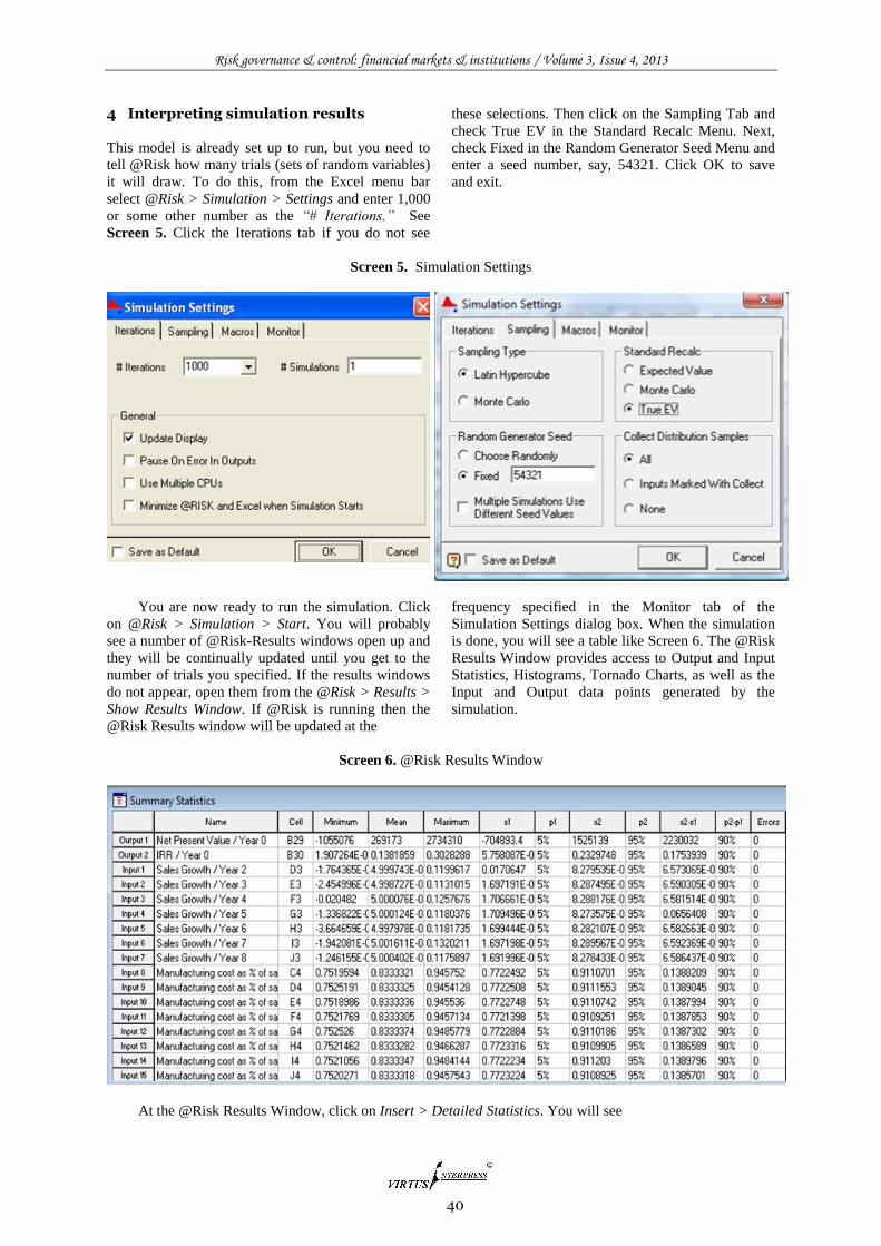
4 Interpreting simulation results

This model is already set up to run, but you need to

tell @Risk how many trials (sets of random variables)

it will draw. To do this, from the Excel menu bar

select @Risk > Simulation > Settings and enter 1,000

or some other number as the “# Iterations.” See

Screen 5. Click the Iterations tab if you do not see

these selections. Then click on the Sampling Tab and

check True EV in the Standard Recalc Menu. Next,

check Fixed in the Random Generator Seed Menu and

enter a seed number, say, 54321. Click OK to save

and exit.

Screen 5. Simulation Settings

You are now ready to run the simulation. Click

on @Risk > Simulation > Start. You will probably

see a number of @Risk-Results windows open up and

they will be continually updated until you get to the

number of trials you specified. If the results windows

do not appear, open them from the @Risk > Results >

Show Results Window. If @Risk is running then the

@Risk Results window will be updated at the

frequency specified in the Monitor tab of the

Simulation Settings dialog box. When the simulation

is done, you will see a table like Screen 6. The @Risk

Results Window provides access to Output and Input

Statistics, Histograms, Tornado Charts, as well as the

Input and Output data points generated by the

simulation.

Screen 6. @Risk Results Window

At the @Risk Results Window, click on Insert > Detailed Statistics. You will see


41

Screen 7. Detailed Statistics

In this table, the mean of output cell B29 is μPV

= $269,173. This provides an estimate of the project

NPV. The standard deviation of output cell B29 is

σNPV = $707,489. This provides an estimate of the

standard deviation of the project NPV. Given μNPV

and σNPV, the 95% confidence interval for the present

value is μNPV +/- 1.96*σNPV/ √N, where N equals the

number of iterations in the simulation. The mean of

output cell B30 is μIRR = 0.1381. This provides an

estimate of the average project IRR.

Suppose you want to determine the probability

that the NPV will be less than $1,000 or be greater

than $2,000. To answer this question, right-click the

B42-Net Present Value/Year output item on the left

panel of the @Risk Results Window.

Screen 8. @Risk Results Window

Then, choose Histogram>Area Graph. You will see screen 9.


42

Screen 9. Histogram of Project NPV

Now go to the right panel and set “Left X” to 0,

and “Right X” to 1500000. You will notice that “Left

P” becomes 41.33%. This corresponds to the

probability that X (here, the NPV) is negative. “Right

P” becomes 94.09%. This corresponds to the

probability that X is less than 1500000. This means

that the probability that X is greater than $1,500,000

is 5.91% =100% - 94.01%.

4.1 Tornado Chart

The tornado chart shows the ranking of different input

variables in terms of their influence on an output

variable. For example, right click B29 – Net Present

Value output item on the left panel of the @Risk

Results Window. Then click on Tornado Chart. See

Screen 10. In the example, sales in year 1 have

considerably more bearing on the distribution of the

NPV any other uncertain variable. This suggests that,

more than anything else, project success hinges on

initial sales. In terms of influence on the NPV, initial

sales is followed by manufacturing cost as a

percentage of sales, sales growth rates, and finally by

the salvage value of fixed assets. Also, consistent with

the time value of money, manufacturing cost as a

percentage of sales in earlier years has more influence

on the distribution of NPV than manufacturing cost as

a percentage of sales in later years. The same thing is

true with the influence on the NPV of sales growth

rate in earlier years compared with later years.

Screen 10. Tornado Chart: Project NPV


43

Simulation results may be reported directly in

Excel using @Risk > Results > Report Setting, at

which point you should see Screen 11. Choose the

options you want for the report and click on the

Generate Reports Now button. @Risk will generate

an Excel report that you can print out. You can save

the results using @Risk > File > Save from the menu

bar. The next time you open the Excel file, you will

have the option to reload the saved simulation results.

Screen 11. Report Settings

5 Concluding remarks

Traditionally, risk is recognized by performing

sensitivity analysis, that is, by examining the impact

on performance variables like NPV or IRR of

deviations in the values of uncertain variables like

sales, sales level, sales growth rates, or unit variable

cost. Simulation modeling allows a more focused

analysis by incorporating explicit distributions

restricting the frequency and magnitude of these

deviations. It is also more general in that it allows the

evaluation of simultaneous changes in uncertain

variables on the distribution of the performance

variables. More useful simulation analysis also is

made possible by the availability of spreadsheet-

based simulation software which allows the analyst to

employ distributions which better reflect the

dynamics of an uncertain variable, instead of force-

fitting more familiar distributions to avoid the

analytical complexity of more realistic distributions.

References 1. Benninga, S., 2006, Principles of Finance with Excel,

(New York: Oxford University Press).

2. Clemen, R. and Reilly, T., 2001, Making Hard

Decisions, (USA: Duxbury).

3. Sheridan Titman and John Martin (2011), “Project Risk

Analysis,” Valuation: The Art and Science of

Corporate Investment Decisions, 2nd ed., Chapter 3,

(Boston, Massachusetts: Pearson/Addison Wesley).

4. Winston, W., Albright, C., and Broadie, M., 2001,

Practical Management Science, 2nd ed., (USA:

Brooks/Cole).


44

APPENDIXMilk4All Project

Year 0 Year 1 Year 2 Year 3 Year 4 Year 5 Year 6 Year 7 Year 8

Sales Growth 0.05 0.05 0.05 0.05 0.05 0.05 0.05

Manufacturing cost as % of sales 0.83 0.83 0.83 0.83 0.83 0.83 0.83 0.83

Rent Increase 0.04 0.04 0.04 0.04 0.04 0.04 0.04 0.04

Sales 4000000 =C7*EXP(D3) =D7*EXP(E3) =E7*EXP(F3) =F7*EXP(G3) =G7*EXP(H3) =H7*EXP(I3) =I7*EXP(J3)

Manufacturing Costs =0.8*C7 =0.8*D7 =0.8*E7 =0.8*F7 =0.8*G7 =0.8*H7 =0.8*I7 =0.8*J7

Rent 100000 =C10*(1+C5) =D10*(1+D5) =E10*(1+E5) =F10*(1+F5) =G10*(1+G5) =H10*(1+H5) =I10*(1+I5)

Total Operating Expenses =C9+C10 =D9+D10 =E9+E10 =F9+F10 =G9+G10 =H9+H10 =I9+I10 =J9+J10

EBITDA =C7-C11 =D7-D11 =E7-E11 =F7-F11 =G7-G11 =H7-H11 =I7-I11 =J7-J11

Depreciation =C38 =D38 =E38 =F38 =G38 =H38 =I38 =J38

EBIT =C13-C15 =D13-D15 =E13-E15 =F13-F15 =G13-G15 =H13-H15 =I13-I15 =J13-J15

Tax Rate 0.35 =C17 =D17 =E17 =F17 =G17 =H17 =I17

Tax =C16*C17 =D16*D17 =E16*E17 =F16*F17 =G16*G17 =H16*H17 =I16*I17 =J16*J17

Net Operating Profit After Taxes =C16-C18 =D16-D18 =E16-E18 =F16-F18 =G16-G18 =H16-H18 =I16-I18 =J16-J18

Depreciation =C15 =D15 =E15 =F15 =G15 =H15 =I15 =J15

Invest. in Net Working Capital =B34 =C34 =D34 =E34 =F34 =G34 =H34 =I34 =J34

Investment In Plant and Equipment =B37 =-J46

Free Cash Flow =B19+B21-B22-B23 =C19+C21-C22-C23 =D19+D21-D22-D23 =E19+E21-E22-E23 =F19+F21-F22-F23 =G19+G21-G22-G23 =H19+H21-H22-H23 =I19+I21-I22-I23 =J19+J21-J22-J23

Cumulative FCF =B25 =B26+C25 =C26+D25 =D26+E25 =E26+F25 =F26+G25 =G26+H25 =H26+I25 =I26+J25

Cost of Capital 0.12

Net Present Value =NPV(B28,C25:J25)+B25

IRR =IRR(B25:J25)

Projected NWC Level 400000 =0.1*D7 =0.1*E7 =0.1*F7 =0.1*G7 =0.1*H7 =0.1*I7 =0.1*J7 =0.1*K7

Investment in NWC =B33 =C33-B33 =D33-C33 =E33-D33 =F33-E33 =G33-F33 =H33-G33 =I33-H33 =J33-I33

Plant & Equipment 2500000 =B37 =C37 =D37 =E37 =F37 =G37 =H37 =I37

Depreciation =C37/10 =D37/10 =E37/10 =F37/10 =G37/10 =H37/10 =I37/10 =J37/10

Accumulated Depreciation =B39+C38 =C39+D38 =D39+E38 =E39+F38 =F39+G38 =G39+H38 =H39+I38 =I39+J38

Ending Book Value of PPE =C37-C39 =D37-D39 =E37-E39 =F37-F39 =G37-G39 =H37-H39 =I37-I39 =J37-J39

Salvage Value of Plant & Equipment 400000

Ending Book Value =J40

Capital Gains =J42-J43

Capital Gains Tax (40%) =0.4*J44

Net Proceeeds from Sale of PPE =J43-J45

Documents

INTRODUCING RISK MODELING IN CORPORATE FINANCE