Introduction to Oracle SQL TuningBobby Durrett

Introduction

“Tuning a SQL statement” means making the SQL query run as fast as you need it to. Inmany cases this means taking a long running query and reducing its run time to a smallfraction of its original length - hours to seconds for example. Books have been written onthis topic and saying something useful in a short paper seems impossible. Oracle’sdatabase software has so many options. What should we talk about first? We contendthat at the core of SQL tuning are three fundamental concepts - join order, join method,and access method. This paper will explain these three concepts and show that tuningSQL boils down to making the proper choice in each category. It is hard to imagine anarea of SQL tuning that doesn’t touch on one or more of these three areas and in any casethe author knows from experience that tuning the join order, join methods, and accessmethods consistently leads to fantastic results.

The following example will be used throughout this paper. It was chosen because it joinsthree tables. Fewer wouldn’t show everything needed, and more would be too complex.

First, here are our three tables in a fictional sales application:

create table sales(sale_date date,product_number number,customer_number number,amount number);

create table products(product_number number,product_type varchar2(12),product_name varchar2(12));

create table customers(customer_number number,customer_state varchar2(14),customer_name varchar2(17));

The sales table has one row for each sale which is one product to one customer for agiven amount. The products and customers tables have one row per product or customer.The columns product_number and customer_number are used to join the tables together.They uniquely identify one product or customer.

Here is the sample data:

insert into sales values (to_date('01/02/2012','MM/DD/YYYY'),1,1,100);insert into sales values (to_date('01/03/2012','MM/DD/YYYY'),1,2,200);insert into sales values (to_date('01/04/2012','MM/DD/YYYY'),2,1,300);insert into sales values (to_date('01/05/2012','MM/DD/YYYY'),2,2,400);

insert into products values (1,'Cheese','Chedder');insert into products values (2,'Cheese','Feta');

insert into customers values (1,'FL','Sunshine State Co');insert into customers values (2,'FL','Green Valley Inc');

Here is our sample query that we will use throughout and its output:

SQL> select2 sale_date, product_name, customer_name, amount3 from sales, products, customers4 where5 sales.product_number=products.product_number and6 sales.customer_number=customers.customer_number and7 sale_date between8 to_date('01/01/2012','MM/DD/YYYY') and9 to_date('01/31/2012','MM/DD/YYYY') and10 product_type = 'Cheese' and11 customer_state = 'FL';

SALE_DATE PRODUCT_NAME CUSTOMER_NAME AMOUNT--------- ------------ ----------------- ----------04-JAN-12 Feta Sunshine State Co 30002-JAN-12 Chedder Sunshine State Co 10005-JAN-12 Feta Green Valley Inc 40003-JAN-12 Chedder Green Valley Inc 200

This query returns the sales for the month of January 2012 for products that are a type ofcheese and customers that reside in Florida. It joins the sales table to products andcustomers to get the product and customer names and uses the product_type andcustomer_state columns to limit the sales records by product and customer criteria.

Join Order

The Oracle optimizer translates this query into an execution tree that represents readsfrom the underlying tables and joins between two sets of row data at a time. Rows mustbe retrieved from the sales, products, and customers tables. These rows must be joinedtogether, but only two at a time. So, sales and products could be joined first and then theresult could be joined to customers. In this case the “join order” would be sales,products, customers.

Some join orders have much worse performance than others. Consider the join ordercustomers, products, sales. This means first join customers to products and then join theresult to sales.

Note that there are no conditions in the where clause that relate the customers andproducts tables. A join between the two makes a Cartesian product which meanscombine each row in products with every row in customers. The following query joinscustomers and products with the related conditions from the original query, doing aCartesian join.

productscustomers

join 1 sales

join 2

productssales

join 1 customers

join 2

SQL> -- joining products and customersSQL> -- cartesian joinSQL>SQL> select

2 product_name,customer_name3 from products, customers4 where5 product_type = 'Cheese' and6 customer_state = 'FL';

PRODUCT_NAME CUSTOMER_NAME------------ -----------------Chedder Sunshine State CoChedder Green Valley IncFeta Sunshine State CoFeta Green Valley Inc

Execution Plan----------------------------------------------------------

0 SELECT STATEMENT Optimizer=ALL_ROWS1 0 MERGE JOIN (CARTESIAN)2 1 TABLE ACCESS (FULL) OF 'PRODUCTS' (TABLE)3 1 BUFFER (SORT)4 3 TABLE ACCESS (FULL) OF 'CUSTOMERS' (TABLE)

In our case we have two products and two customers so this is just 2 x 2 = 4 rows. Butimagine if you had 100,000 of each. Then a Cartesian join would return 100,000 x100,000 = 10,000,000,000 rows. Probably not the most efficient join order. But, if youhave a small number of rows in both tables there is nothing wrong with a Cartesian joinand in some cases this is the best join order. But, clearly there are cases where aCartesian join blows up a join of modest sized tables into billions of resulting rows andthis is not the best way to optimize the query.

There are many possible join orders. If the variable n represents the number of tables inyour from clause there are n! possible join orders. So, our example query has 3! = 6 joinorders:

sales, products, customerssales, customers, productsproducts, customers, salesproducts, sales, customerscustomers, products, salescustomers, sales, products

The number of possible join orders explodes as you increase the number of tables in thefrom clause:

Tables in fromclause

Possible joinorders

1 1

2 2

3 6

4 24

5 120

6 720

7 5040

8 40320

9 362880

10 3628800

You might wonder if these join orders were really different:

sales, products, customersproducts, sales, customers

In both cases sales and products are joined first and then the result is joined to customers:

Join order 1:

productssales

join 1 customers

join 2

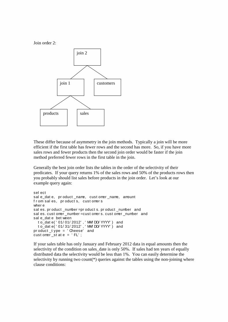
Join order 2:

These differ because of asymmetry in the join methods. Typically a join will be moreefficient if the first table has fewer rows and the second has more. So, if you have moresales rows and fewer products then the second join order would be faster if the joinmethod preferred fewer rows in the first table in the join.

Generally the best join order lists the tables in the order of the selectivity of theirpredicates. If your query returns 1% of the sales rows and 50% of the products rows thenyou probably should list sales before products in the join order. Let’s look at ourexample query again:

selectsale_date, product_name, customer_name, amountfrom sales, products, customerswheresales.product_number=products.product_number andsales.customer_number=customers.customer_number andsale_date between

to_date('01/01/2012','MM/DD/YYYY') andto_date('01/31/2012','MM/DD/YYYY') and

product_type = 'Cheese' andcustomer_state = 'FL';

If your sales table has only January and February 2012 data in equal amounts then theselectivity of the condition on sales_date is only 50%. If sales had ten years of equallydistributed data the selectivity would be less than 1%. You can easily determine theselectivity by running two count(*) queries against the tables using the non-joining whereclause conditions:

salesproducts

join 1 customers

join 2

-- # selected rows

selectcount(*)from saleswheresale_date between

to_date('01/01/2012','MM/DD/YYYY') andto_date('01/31/2012','MM/DD/YYYY');

-- total #rows

selectcount(*)from sales;

You should do this for every table in the from clause to see the real selectivity.

In the same way, you need to know the selectivity of each subtree in the plan - i.e. eachcombination of tables that have already been joined together. So, in our three tableexample this would just be the three possible combinations - sales and products, sales andcustomers, and customers and products. Here is the sales and products combination:

SQL> select count(*)2 from sales, products3 where4 sales.product_number=products.product_number and5 sale_date between6 to_date('01/01/2012','MM/DD/YYYY') and7 to_date('01/31/2012','MM/DD/YYYY') and8 product_type = 'Cheese';

COUNT(*)----------

4

SQL> select count(*)2 from sales, products3 where4 sales.product_number=products.product_number;

COUNT(*)----------

4

In this simple example the selectivity of the sales and products combination is 100%because the count without the conditions against the constants equals the count with theconditions with constants. But, in a real query these would differ and in some cases thecombination of conditions on two tables is much more selective than the conditions oneach individual table.

Extreme differences in selectivity cause reordering the joins to produce the best tuningimprovement. We started out this paper with the idea that you have a SQL statement that

is slow and you want to speed it up. You may want a query that runs for hours to run inseconds. To find this kind of improvement by looking at join order and predicateselectivity you have to look for a situation where the predicates on one of the tables hasan extremely high selectivity compared with the others. So, say your conditions on yoursales rows reduced the number of sales rows considered down to a handful of rows out ofthe millions in the table. Putting the sales table first in the join order if it isn’t already putthere by the optimizer could produce a huge improvement, especially if the conditions onthe other large tables in the join were not very selective. What if your criteria forproducts reduced you down to one product row out of hundreds of thousands? Putproducts first. On the other hand if there isn’t a big gap in the selectivity against thetables in the from clause then simply ordering the joins by selectivity is not guaranteed tohelp.

You change the join order by giving the optimizer more information about the selectivityof the predicates on the tables or by manually overriding the optimizer’s choice. If theoptimizer knows that you have an extremely selective predicate it will put the associatedtable at the front of the join order. You can help the optimizer by gathering statistics onthe tables in the from clause. Accurate statistics help the optimizer know how selectivethe conditions are. In some cases higher estimate percentages on your statistics gatheringcan make the difference. In other cases histograms on the columns that are so selectivecan help the optimizer realize how selective the conditions really are.

Here is how to set the optimizer preferences on a table to set the estimate percentage andchoose a column to have a histogram and gather statistics on the table:

-- 1 - set preferences

begin

DBMS_STATS.SET_TABLE_PREFS(NULL,'SALES','ESTIMATE_PERCENT','10');DBMS_STATS.SET_TABLE_PREFS(NULL,'SALES','METHOD_OPT',

'FOR COLUMNS SALE_DATE SIZE 254 PRODUCT_NUMBER SIZE 1 '||'CUSTOMER_NUMBER SIZE 1 AMOUNT SIZE 1');

end;/

-- 2 - regather table stats with new preferences

execute DBMS_STATS.GATHER_TABLE_STATS (NULL,'SALES');

This set the estimate percentage to 10% for the sales table. It put a histogram on thesales_date column only.

You can use a cardinality hint to help the optimizer know which table has the mostselective predicates. In this example we tell the optimizer that the predicates on the salestable will only return one row:

SQL> select /*+cardinality(sales 1) */2 sale_date, product_name, customer_name, amount3 from sales, products, customers4 where5 sales.product_number=products.product_number and6 sales.customer_number=customers.customer_number and7 sale_date between8 to_date('01/01/2012','MM/DD/YYYY') and9 to_date('01/31/2012','MM/DD/YYYY') and10 product_type = 'Cheese' and11 customer_state = 'FL';

SALE_DATE PRODUCT_NAME CUSTOMER_NAME AMOUNT--------- ------------ ----------------- ----------04-JAN-12 Feta Sunshine State Co 30002-JAN-12 Chedder Sunshine State Co 10005-JAN-12 Feta Green Valley Inc 40003-JAN-12 Chedder Green Valley Inc 200

Execution Plan----------------------------------------------------------

0 SELECT STATEMENT Optimizer=ALL_ROWS1 0 HASH JOIN2 1 HASH JOIN3 2 TABLE ACCESS (FULL) OF 'SALES' (TABLE)4 2 TABLE ACCESS (FULL) OF 'PRODUCTS' (TABLE5 1 TABLE ACCESS (FULL) OF 'CUSTOMERS' (TABLE)

As a result, the optimizer puts sales at the beginning of the join order. Note that in thiscase for an example we lied to the optimizer since really there are four rows. Sometimesgiving the optimizer the true cardinality will work, but in others you will need to under oroverestimate to get the join order that is optimal.

You can use a leading hint to override the optimizer’s choice of join order. For exampleif sales had the highly selective predicate you could do this:

SQL> select /*+leading(sales) */2 sale_date, product_name, customer_name, amount3 from sales, products, customers4 where5 sales.product_number=products.product_number and6 sales.customer_number=customers.customer_number and7 sale_date between8 to_date('01/01/2012','MM/DD/YYYY') and9 to_date('01/31/2012','MM/DD/YYYY') and10 product_type = 'Cheese' and11 customer_state = 'FL';

SALE_DATE PRODUCT_NAME CUSTOMER_NAME AMOUNT--------- ------------ ----------------- ----------04-JAN-12 Feta Sunshine State Co 30002-JAN-12 Chedder Sunshine State Co 10005-JAN-12 Feta Green Valley Inc 40003-JAN-12 Chedder Green Valley Inc 200

Execution Plan----------------------------------------------------------

0 SELECT STATEMENT Optimizer=ALL_ROWS1 0 HASH JOIN2 1 HASH JOIN3 2 TABLE ACCESS (FULL) OF 'SALES' (TABLE)4 2 TABLE ACCESS (FULL) OF 'PRODUCTS'5 1 TABLE ACCESS (FULL) OF 'CUSTOMERS' (TABLE)

The leading hint on sales forced it to be the first table in the join order just like thecardinality hint. It left it up to the optimizer to choose either products or customers as thenext table.

If all else fails and you can’t get the optimizer to join the tables together in an efficientorder you can break the query into multiple queries saving the intermediate results in aglobal temporary table. Here is how to break our three table join into two joins - firstsales and products, and then the results of that join with customers:

SQL> create global temporary table sales_product_results2 (3 sale_date date,4 customer_number number,5 amount number,6 product_type varchar2(12),7 product_name varchar2(12)8 ) on commit preserve rows;

Table created.

SQL> insert /*+append */2 into sales_product_results3 select4 sale_date,5 customer_number,6 amount,7 product_type,8 product_name9 from sales, products10 where11 sales.product_number=products.product_number and12 sale_date between13 to_date('01/01/2012','MM/DD/YYYY') and14 to_date('01/31/2012','MM/DD/YYYY') and15 product_type = 'Cheese';

4 rows created.

SQL> commit;

Commit complete.

SQL> select2 sale_date, product_name, customer_name, amount3 from sales_product_results spr, customers c4 where5 spr.customer_number=c.customer_number and6 c.customer_state = 'FL';

SALE_DATE PRODUCT_NAME CUSTOMER_NAME AMOUNT--------- ------------ ----------------- ----------02-JAN-12 Chedder Sunshine State Co 10003-JAN-12 Chedder Green Valley Inc 20004-JAN-12 Feta Sunshine State Co 30005-JAN-12 Feta Green Valley Inc 400

Breaking a query up like this is a very powerful method of tuning. If you have the abilityto modify an application in this way you have total control over how the query is runbecause you decide which joins are done and in what order. I’ve seen dramatic run timeimprovement using this simple technique.

Join Methods

The choice of the best join method is determined by the number of rows being joinedfrom each source and the availability of an index on the joining columns. Nested loopsjoins work best when the first table in the join has few rows and the second has a uniqueindex on the joined columns. If there is no index on the larger table or if both tables havea large number of rows to be joined then hash join them with the smaller table first in thejoin.

Here is our sample query’s plan with all nested loops:

Execution Plan----------------------------------------------------------

0 SELECT STATEMENT Optimizer=ALL_ROWS1 0 TABLE ACCESS (BY INDEX ROWID) OF 'CUSTOMERS' (TABLE)2 1 NESTED LOOPS3 2 NESTED LOOPS4 3 TABLE ACCESS (FULL) OF 'SALES' (TABLE)5 3 TABLE ACCESS (BY INDEX ROWID) OF 'PRODUCTS'6 5 INDEX (RANGE SCAN) OF 'PRODUCTS_INDEX' (INDEX)7 2 INDEX (RANGE SCAN) OF 'CUSTOMERS_INDEX' (INDEX)

In this example let’s say that the date condition on the sales table means that only a fewrows would be returned from sales. But, what if the conditions on products andcustomers were not very limiting? Maybe all your customers are in Florida and youmainly sell cheese. If you have indexes on product_number and customer_number or ifyou add them then a nested loops join makes sense here.

But, what if the sales table had many rows in the date range the conditions on productsand customers were not selective either? In this case the nested joops join using theindex can be very inefficient. We have seen many cases were doing a full scan on both

tables in a join and using a hash join produces the fastest query runtime. Here is a planwith all hash joins that we saw in our leading hint example:

Execution Plan----------------------------------------------------------

0 SELECT STATEMENT Optimizer=ALL_ROWS1 0 HASH JOIN2 1 HASH JOIN3 2 TABLE ACCESS (FULL) OF 'SALES' (TABLE)4 2 TABLE ACCESS (FULL) OF 'PRODUCTS'5 1 TABLE ACCESS (FULL) OF 'CUSTOMERS' (TABLE)

Of course you can mix and match and use a hash join in one case and nested loops inanother.

Execution Plan----------------------------------------------------------

0 SELECT STATEMENT Optimizer=ALL_ROWS1 0 TABLE ACCESS (BY INDEX ROWID) OF 'CUSTOMERS' (TABLE)2 1 NESTED LOOPS3 2 HASH JOIN4 3 TABLE ACCESS (FULL) OF 'SALES' (TABLE)5 3 TABLE ACCESS (FULL) OF 'PRODUCTS' (TABLE)6 2 INDEX (RANGE SCAN) OF 'CUSTOMERS_INDEX' (INDEX)

As with join order you can cause the optimizer to use the optimal join method by eitherhelping it know how many rows will be joined from each row source or by forcing thejoin method using a hint. The following hints forced the join methods used above:

/*+ use_hash(sales products) use_nl(products customers) */

Use_hash forces a hash join, use_nl forces a nested loops join. The table with the fewestrows to be joined should go first. A great way to get the optimizer to use a nested loopsjoin is to create an index on the join columns of the table with the least selective whereclause predicates. For example, these statements create indexes on the product_numberand customer_number columns of the products and customers tables:

create index products_index on products(product_number);create index customers_index on customers(customer_number);

You can encourage hash joins by manually setting the hash_area_size to a large number.The init parameter hash_area_size is an area of memory in each session’s serverprocess’s local memory (PGA) that buffers the on-disk hash table. The more memorydedicated to hashing the more efficient a hash join is and the more likely the optimizer isto choose a hash join over a nested loops join. You have to first turn off automatic pgamemory management by setting workarea_size_policy to manual and then setting sortand hash area sizes.

Here is an example from a working production system:

NAME TYPE VALUE------------------------------------ ----------- ---------hash_area_size integer 100000000sort_area_size integer 100000000workarea_size_policy string MANUAL

Access Methods

For clarity we limit our discussion of access method to two options: index scan and fulltable scan. There are many possible access methods but at its core the choice of accessmethod comes down to how many rows will be retrieved from the table. Access a tableusing an index scan when you want to read a very small percentage of the rows,otherwise use a full table scan. An old rule of thumb was that if you read 10% of thetable or less use an index scan. Today that rule should be 1% or even much less. If youare accessing only a handful of rows of a huge table and you are not using an index thenswitch to an index. If the table is small or if you are accessing even a modest percentageof the rows you will want a full scan.

The parameters optimizer_index_caching, optimizer_index_cost_adj, anddb_file_multiblock_read_count all affect how likely the optimizer is to use an indexversus a full scan. You may find that you have many queries using indexes where a fullscan is more efficient or vice versa. These parameters can improve the performance ofmany queries since they are system wide. On one Exadata system where we wanted todiscourage index use we set optimizer_index_cost_adj to 1000, ten times its normalsetting of 100. This caused many queries to begin using full scans, which Exadataprocesses especially well. Here is the command we used to set this parameter value:

alter system set optimizer_index_cost_adj=1000 scope=both sid='*';

The greater the degree of parallelism set on a table the more likely the optimizer is to usea full scan. So, if a table is set to parallel 8 the optimizer assumes a full scan takes 1/8th

the time it would serially. But there are diminishing marginal returns on increasing thedegree of parallelism. You get less benefit as you go above 8 and if you have many usersquerying with a high degree of parallelism you can overload your system. This is howyou set a table to a parallel degree 8:

alter table sales parallel 8;

Last, but certainly not least in importance are index and full scan hints. Here areexamples of both:

/*+ full(sales) index(customers) index(products) */

These hints force the sales table to be accessed using a full scan, but require thecustomers and products tables to be accessed using an index.

Conclusion

We have demonstrated how to tune an Oracle SQL query by examining and manipulatingthe join order, join methods, and access methods used in the query’s execution plan. Firstyou must query the tables to determine the true number of rows returned from each tableand from each likely join. Then you identify which join order, join method, or accessmethod chosen by the optimizer is inefficient. Then you use one of the suggestedmethods to change the optimizer’s choice to be the efficient one. These methods includegathering optimizer statistics, hints, setting init parameters, breaking the query intosmaller pieces, and adjusting the parallel degree. Left unsaid is that you must test yourchanged plan to make sure the new combination of join order, join methods and accessmethods actually improve the performance. In SQL*Plus turn timing on and check theelapsed time with the optimizer’s original execution plan and compare the elapsed timewith the new plan:

SQL> set timing onSQL>SQL> select

2 sale_date, product_name, customer_name, amount3 from sales, products, customers4 where5 sales.product_number=products.product_number and6 sales.customer_number=customers.customer_number and7 sale_date between8 to_date('01/01/2012','MM/DD/YYYY') and9 to_date('01/31/2012','MM/DD/YYYY') and10 product_type = 'Cheese' and11 customer_state = 'FL';

SALE_DATE PRODUCT_NAME CUSTOMER_NAME AMOUNT--------- ------------ ----------------- ----------02-JAN-12 Chedder Sunshine State Co 10003-JAN-12 Chedder Green Valley Inc 20004-JAN-12 Feta Sunshine State Co 30005-JAN-12 Feta Green Valley Inc 400

Elapsed: 00:00:00.00

This is the final test that our analysis has brought us to our initial goal - of vastlyimproved run time for our problem query.

Here are some suggestions for further reading to flesh out the details from this paper:

Oracle Database Concepts 11g Release 2 (11.2)

Chapter 7 SQL - overview of SQL processing and execution plans

Oracle Database Performance Tuning Guide 11g Release 2 (11.2)

Chapter 11 The Query Optimizer - more details on plans and hintsChapter 19 Using Optimizer Hints - details on hints

Oracle Database Reference 11g Release 2 (11.2)

Chapter 1 Initialization Parameters - details on the init.ora parameters from this paper

Oracle Database PL/SQL Packages and Types Reference Release 2 (11.2)

Chapter 141 DBMS_STATS - statistics gathering procedures and their arguments

Cost-Based Oracle Fundamentals - Jonathan Lewis

This book contains a very helpful and in-depth explanation of how the Oracle optimizerworks. Highly recommended