Intro to Longitudinal Data: A Grad Student “How-To” Paper Elisa L. Priest1,2 , Ashley W. Collinsworth1,3

1 Institute for Health Care Research and Improvement, Baylor Health Care System 2 University of North Texas School of Public Health

3 Tulane University

ABSTRACT

Grad students learn the basics of SAS programming in class or on their own. Although students may deal with longitudinal data in class, the lessons focus on statistical procedures and the datasets are usually ready for analysis. However, longitudinal data may be organized in many complex structures, especially if it was collected in a relational database. Once students begin working with ‘real’ longitudinal data, they quickly realize that manipulating the data so it can be analyzed is its own time consuming challenge. In the real world of messy data, we often spend more time preparing the data than performing the analysis. Students need tools that can help them survive the challenges of working with longitudinal data. These challenges include combining datasets, counting repeat observations, performing calculations across records, and restructuring repeating data from multiple observations to single observation. This paper will use real world examples from grad students to demonstrate useful functions, FIRST. and LAST. variables, and how to transform datasets using PROC TRANSPOSE. This paper is the fifth in the ‘Grad Student How-To’ series and gives graduate students useful tools for working with longitudinal data.

OUTLINE

1. Introduction

2. Datasets

3. Planning

4. Merging

5. Counting

6. Restructuring

7. Calculations across records

8. Finalizing the analysis dataset

9. Conclusions

INTRODUCTION

Grad students often rely on existing datasets for research projects. They are expected to formulate a research question, review the available data sources, prepare data for analysis, and perform the analysis. Longitudinal data is collected across multiple time points and is common in research. Having multiple time points is useful for analysis, but increases the complexity of the data organization and management. This paper describes the processes and challenges of preparing a longitudinal data set for analysis. The goal of the research project is to compare the baseline visit laboratory values with the final visit laboratory values.

DATASETS

The data is organized in four files that were obtained from two different data sources. The participants, visits, and participant_visits tables were part of a relational database designed in Microsoft Access to track and store information about the study. The labs table was obtained from a separate laboratory information system (LIMS).

Participants: The participants table contains one record for each participant and includes participantID, gender, race, date_program_start

Visits: The visits table contains one record for each visit for each participant and includes a visitID, visitdate, and visitname

Participant_visits: The participant_visits table contains one record for each visit for each participant and includes the participantID and visitID. This table is used to tie together the participants and visits tables.

Labs: The labs table was obtained from a laboratory information system (LIMS) and contains one record for each lab test done for each participant at each visit and includes an ID_patient, exam_date, test, and value.

Participants Labs

Participants_visits Visits

PLANNING

This project requires that we look at change in laboratory values over time in the study participants. We need to create a plan to combine the four datasets into an analysis dataset. First, we may use a PROC CONTENTS to examine the available variables and their formats. In the code below, OUT=work.contents_participants creates a dataset of the PROC CONTENTS output. This is useful for documentation purposes and can easily be exported to Microsoft Excel. The option POSITION puts the variables in order of their position in the dataset instead of alphabetically.

proc contents data=work.participants out=work.contents_participants position; run;

Portion of work.contents_participants

Next, we look for common variables and formats across tables. We also open each table and look at the structure of the data. After reviewing the data, several important facts arise:

The labs table uses a different ID than the participants table.

The labs table does not contain a visitID variable

The labs table has many records for each participant and exam date.

The visits table does not contain a participantID variable.

This is not going to be as easy as it first seemed!

The basic plan is to:

Merge the participant_visits table with the visits table. This will allow us to have a common variable across the tables.

Count the number of visits for each participant and summarize across all participants.

Count the number of lab measurements for each participant and summarize across all participants.

Restructure the labs table to have one record per participant visit

Calculate differences in labs across visits

Calculate the differences in labs between first and last visit

Merge tables together for final analyses

MERGING

The first two datasets that we need to merge are the participant_visits table and the visits table. The common variable between the two tables is the visitID. First, use a PROC SORT to sort by visitID and then use a data step with MERGE statement to merge the two datasets by visitID. After merging, sort the dataset by participantID and visitdate to put the visits in an order that makes sense. Our data now has the participantID plus the visit information.

proc sort data=work.participant_visits; by visitID; run; proc sort data=work.visits; by visitID; run; data work.visits_all; merge work.participant_visits work.visits; by visitID; run; proc sort data=work.visits_all; by participantID visitdate; run;

COUNTING

We see that each participant has up to seven visits. However, it is possible that some participants may have less than seven visits. To confirm this, use a PROC FREQ to get a frequency count on the number of visits.

proc freq data=work.visits_all; table visitname; run;

We need to count the number of visits that are present for each participant. We could take the last visit name for each participant. However, this assumes that there are no missing visits for that participant. Instead, we will use the BY group processing in a DATA step with a counter variable. When we use the BY group, SAS creates two temporary variables: FIRST.variable and LAST.variable that identify the first and last values for a variable. For our dataset, we can use this to count the number of visits for each participant. The table below shows the temporary variables that SAS is using behind the scenes. You can see that the first record for participantID has the FIRST. flag =1.

Since the data is already sorted by participantID, we use a DATA step and BY participantID to tell SAS to create two temporary variables: FIRST.participantID and LAST.participantID. We also create a new variable to count the records, visit_count. We use the RETAIN statement so that SAS keeps the value of visit_count as it moves to the next observation. We use the FIRST. variable to set visit_count=0 every time SAS encounters a new participantID. We can see from the output that each visit_count incremements by 1 for each visit record listed and then resets when the next participantID is encountered.

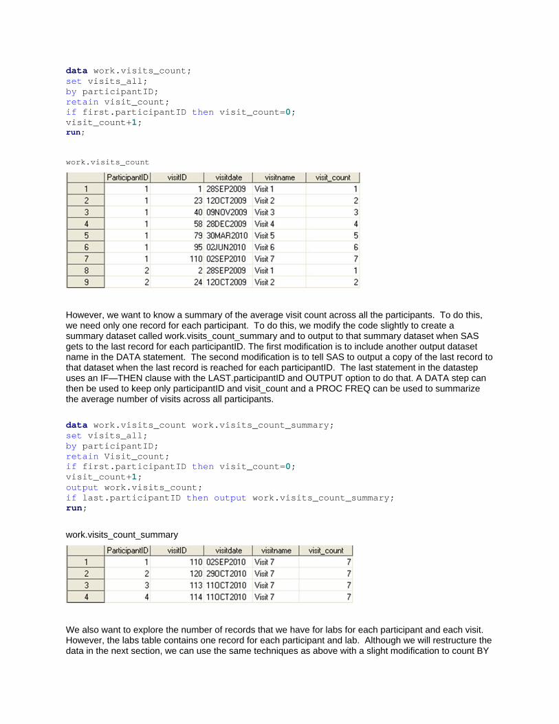
data work.visits_count; set visits_all; by participantID; retain visit_count; if first.participantID then visit_count=0; visit_count+1; run;

work.visits_count

However, we want to know a summary of the average visit count across all the participants. To do this, we need only one record for each participant. To do this, we modify the code slightly to create a summary dataset called work.visits_count_summary and to output to that summary dataset when SAS gets to the last record for each participantID. The first modification is to include another output dataset name in the DATA statement. The second modification is to tell SAS to output a copy of the last record to that dataset when the last record is reached for each participantID. The last statement in the datastep uses an IF—THEN clause with the LAST.participantID and OUTPUT option to do that. A DATA step can then be used to keep only participantID and visit_count and a PROC FREQ can be used to summarize the average number of visits across all participants.

data work.visits_count work.visits_count_summary; set visits_all; by participantID; retain Visit_count; if first.participantID then visit_count=0; visit_count+1; output work.visits_count; if last.participantID then output work.visits_count_summary; run;

work.visits_count_summary

We also want to explore the number of records that we have for labs for each participant and each visit. However, the labs table contains one record for each participant and lab. Although we will restructure the data in the next section, we can use the same techniques as above with a slight modification to count BY

participantID and exam_date. We review the PROC CONTENTS for the lab table and remember that the lab data came from a different source and has a different unique identified for the participant: ID_patient.

We do a PROC SORT to sort the data by ID_patient and exam_date. Next, we use a DATA step to create a table called work.labs_summary and use the BY statement with ID_patient and exam_date. We reset the counter variable lab_visit_count when both FIRST.ID_patient and FIRST.exam_date =1. The keep statement and the if—then—output statement can also be used to keep only the summary information. We notice that most people have fewer lab visits than other visits, and some have no data!

proc sort data=work.labs; by ID_patient exam_date; run; data work.labs_summary; set work.labs; by ID_patient exam_date; retain lab_visit_count lab_count; if first.ID_patient and first.exam_date then lab_visit_count=0; if first.exam_date then lab_visit_count=lab_visit_count+1; *keep ID_Patient lab_visit_count; *if last.ID_Patient then output;

run;

work.labs_summary with the original code

work.labs_summary with the *commented out code

RESTRUCTURING

After counting the number of visits, we move on to looking more in depth at the lab data. Our goal is to calculate the change in the lab values between visits. In preparation for transposing the data, we need to clean up the dataset a bit. We use the SAS character function SCAN to pull out the first word from the test description. This gives us a short name that can be used for the variable. At the same time, we decide to rename the variables ID_Participant and exam_date to match the other datasets. The RENAME statement easily takes care of this.

data work.labs_names; set work.labs (rename= (ID_patient=participantID exam_Date=visitdate)); test_name=scan(test,1); run;

work.labs_names

Next, we use PROC TRANSPOSE to restructure the dataset from skinny to wide. The OUT= option makes sure that we do not save over our existing dataset. We transpose BY participantID and visitdate to get one record for each visit for each participant. We tell PROC TRANSPOSE to transpose the value variable and the ID statement tells SAS to use the short description in test_name for the new variables and PREFIX=value tells SAS to put a prefix on the front of each variable name5.

proc transpose data=work.labs_names out=work.labs_transpose prefix=value_; by participantID visitdate; var value; ID test_name; run;

work.labs_transpose

Problem data.

The data appears correct for the first few participants. However, we notice that some individuals have records with no data values for the labs. We decided to delete these records to avoid causing problems in the calculations across records. :

CALCULATIONS ACROSS RECORDS

We have two calculations that we want to perform for hemoglobin values. First, we want to calculate the difference between each successive hemoglobin value. Secondly, we want to calculate the change in

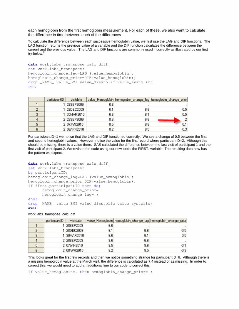
each hemoglobin from the first hemoglobin measurement. For each of these, we also want to calculate the difference in time between each of the differences

To calculate the difference between each successive hemoglobin value, we first use the LAG and DIF functions. The LAG function returns the previous value of a variable and the DIF function calculates the difference between the current and the previous value. The LAG and DIF functions are commonly used incorrectly as illustrated by our first try below.6

data work.labs_transpose_calc_diff; set work.labs_transpose; hemoglobin_change_lag=LAG (value_hemoglobin); hemoglobin_change_prior=DIF(value_hemoglobin); drop _NAME_ value_BMI value_diastolic value_systolic; run;

For participantID=1 we notice that the LAG and DIF functioned correctly. We see a change of 0.5 between the first and second hemoglobin values. However, notice the value for the first record where participantID=2. Although this should be missing, there is a value there. SAS calculated the difference between the last visit of participant 1 and the first visit of participant 2. We revised the code using our new tools: the FIRST. variable. The resulting data now has the pattern we expect.

data work.labs_transpose_calc_diff; set work.labs_transpose; by participantID; hemoglobin_change_lag=LAG (value_hemoglobin); hemoglobin_change_prior=DIF(value_hemoglobin); if first.participantID then do; hemoglobin_change_prior=.; hemoglobin_change_lag=.; end; drop _NAME_ value_BMI value_diastolic value_systolic; run;

work.labs_transpose_calc_diff

This looks great for the first few records and then we notice something strange for participantID=6. Although there is a missing hemoglobin value at the March visit, the difference is calculated as 7.4 instead of as missing. In order to correct this, we would need to add an additional line to our code to correct this.

if value_hemoglobin=. then hemoglobin_change_prior=.;

Next, we need to calculate the change between the current value of hemoglobin and a defined baseline value. For this calculation, we will use a different technique. We will create a flag for the baseline lab value and a new variable for the baseline hemoglobin that we will RETAIN across observations to perform a calculation.

data work.labs_transpose_calc_baseline; set work.labs_transpose; retain hemoglobin_baseline; by participantID visitdate; If first.participantID and first.visitdate then do; baseline_labs_flag=1; hemoglobin_baseline=value_hemoglobin; end; hemoglobin_change_baseline=value_hemoglobin-hemoglobin_baseline; drop _NAME_ value_BMI value_diastolic value_systolic; run;

work.labs_transpose_calc_baseline

Now that we have the code down, we modify it slightly to calculate the difference in the visit dates. We add visitdate_baseline to the retain statement , set it to missing in the if FIRST.participantID statement, and calculate the change by subtracting the visitdate_baseline.

data work.labs_transpose_calc_baseline; set work.labs_transpose; RETAIN hemoglobin_baseline visitdate_baseline; by participantID visitdate; If first.participantID and first.visitdate then do; baseline_labs_flag=1; hemoglobin_baseline=value_hemoglobin; visitdate_baseline=visitdate; end; hemoglobin_change_baseline=value_hemoglobin-hemoglobin_baseline; visitdate_change=visitdate-visitdate_baseline; drop _NAME_ value_BMI value_diastolic value_systolic; run;

Notice that visitdate_baseline is appearing as ‘18168’ instead of 28SEP2009. This is because there is no format for this date value. SAS represents datevalues using a reference date of January 1, 1960 as day 0 for all calculations. Thus, January 2, 1960 is day 1. The value for visitdate_change that is returned is the number of days between the two dates. If we want to see a different interval, for example, number of months, we can use Datetime function called INTCK.7 The format of INTCK is: INTCK ( interval, from, to )

We add the following line to our previous code:

visitdate_change_month=INTCK("MONTH",visitdate_baseline,visitdate);

We see that in the resulting table we have 91 days, or 3 months between the first and second visits for participantID=1. One subtle feature of the INTCK function is that the value that is returned is the number of interval boundries (|| illustrated below) that are crossed. Basically this means there is no rounding of months. For more information about this and other DATETIME fucntions, refer to the SAS User’s guide.7

Interval 1 Interval 2 Interval 3 Interval 4

September-----------|| October---------------||Novemeber----------- || December -------------|| January

Finally, we combine the techniques that we learned into one SAS datastep and add a calculation for difference in date between each visit.

data work.labs_transpose_calc; set work.labs_transpose; *retain statement suesd for calculations*; RETAIN hemoglobin_baseline visitdate_baseline; *by statement creates FIRST. and LAST. temporary variables*; by participantID visitdate; *create baseline flag and initalize baseline values and dates for RETAIN*; If first.participantID and first.visitdate then do; baseline_labs_flag=1; hemoglobin_baseline=value_hemoglobin; visitdate_baseline=visitdate; end; *calculate changes baseline using retained values*; hemoglobin_change_baseline=value_hemoglobin-hemoglobin_baseline; visitdate_change_baseline=visitdate-visitdate_baseline; visitdate_change_month=INTCK("MONTH",visitdate_baseline,visitdate); *calculate changes between current and previous using LAG and DIF*;

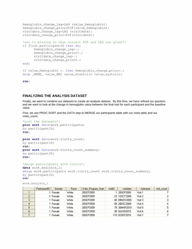
hemoglobin_change_lag=LAG (value_hemoglobin); hemoglobin_change_prior=DIF(value_hemoglobin); visitdate_change_lag=LAG (visitdate); visitdate_change_prior=DIF(visitdate); *set to missing so that correct DIF and LAG are given*; if first.participantID then do; hemoglobin_change_lag=.; hemoglobin_change_prior=.; visitdate_change_lag=.; visitdate_change_prior=.; end; if value_hemoglobin =. then hemoglobin_change_prior=.; drop _NAME_ value_BMI value_diastolic value_systolic; run;

FINALYZING THE ANALYSIS DATASET

Finally, we want to combine our datasets to create an analysis dataset. By this time, we have refined our question and we want to look at the change in hemoglobin value between the final visit for each participant and the baseline value.

First, we use PROC SORT and the DATA step to MERGE our participants table with our visits table and our visits_count.

*sort the datasets*; proc sort data=work.participants; by participantID; run; proc sort data=work.visits_count; by participantID; run; proc sort data=work.visits_count_summary; by participantID; run; *merge participants with visits*; data work.analysis_1; merge work.participants work.visits_count work.visits_count_summary; by participantID; run;

work.analysis_1

Next, we use PROC SORT and the DATA step to MERGE this table with our calculated lab values table. We want to merge by both participantID and visitdate since we have multiple visits in both datasets.

*sort the datasets*; proc sort data=work.analysis_1; by participantID visitdate; run; proc sort data=work.labs_transpose_calc; by participantID visitdate; run; *merge analysis_1 with labs data with calculations*; data work.analysis_2; merge work.analysis_1 work.labs_transpose_calc; by participantID visitdate; run;

This looks great for the first participants. And then, we notice something odd. For some participants, there is not a direct match in the visit dates between the labs and the participant visits table. If we look closely, it appears that the labs were done one day earlier than the date for the participants visits.

We have several different options that we considered here. First, we can match the participant information directly with the labs table and not worry about the visit name information. Another option is to do a fuzzy merge. A fuzzy merge is where the merge values are not exact, but may have a range. In this case, we review the records and decide that a range of 10 days will constitute a match between the clinical visit and the laboratory values. After googling and reviewing the information on support.sas.com, we decide to use PROC SQL to perform the merge.

proc sql; create table work.analysis_3 as select * from analysis_1(rename=(visitdate=visit_participants )) A, labs_transpose_calc(rename=(visitdate=visit_labs ))B Where (A.participantID=B.participantID AND ABS(visit_labs-visit_participants) <= 10); quit;

This method left us with only those visits which had a match on date within 10 days. However, this was fine for our analysis. Our analysis required us to examine the total change from baseline for the hemoglobin values. The final step to prepare our data for analysis was to select only the last data point for each participant.

We notice that not every participantID had laboratory records. This is ok, but we note it in our methods. In addition, we notice that the baseline_labs flag=1 for some participants. This indicates that these participants only had one record of labs. We update our code to remove these participants who have a FIRST.participantID=1.

data work.analysis_final; set work.analysis_3; by participantID; if LAST.participantID; if FIRST.participantID then delete; run;

CONCLUSIONS AND WHERE TO FIND MORE

This paper is the fifth in the ‘Grad Student How-To’ series1,2,3,4 and gives graduate students useful tools for working with longitudinal data. The tools included in this paper were PROC CONTENTS, LAG and DIF functions, basic DATETIME functions, the RETAIN statement, merging datasets, PROC TRANSPOSE, FIRST. and LAST. variables, and a fuzzy merge.

There are many references available to students who are interested in learning more about working with longitudinal data.. First, start at the support.sas.com website to locate papers and documentation. The SAS Language reference for version 9.2 is online at http://support.sas.com/documentation/cdl_main/index.html and allows you to search for a keyword such as ‘LAG’. In addition, you can get to sample code and notes at http://support.sas.com/notes/index.html. There are many useful code samples in this repository. One interesting Usage note that I just came upon is Usage Note 30333:FASTats: Frequently asked for statistics at http://support.sas.com/kb/30/333.html. This note lists statistics procedures and gives useful links. Finally, you can search http://support.sas.com/events/sasglobalforum/previous/online.html for many useful papers from previous SAS Global Users Group conferences.

REFERENCES

1) Priest EL. Keep it Organized- SAS tips for a research project. South Central SAS Users Group 2006 Conference, Irving, TX, October 15-18, 2006.

2) Priest EL, Adams B, Fischbach L. Easier Exploratory Analysis for Epidemiology: A Grad Student How To Paper. SAS Global Forum 2009. Paper 241-2009.

3)Priest EL, Blankenship D. A Grad Student ‘How-To’ Paper on Grant Preparation: Preliminary Data, Power Analysis, and Presentation. SAS Global Forum 2010. Paper 274-2010.

4)Priest EL, Harper JS. Intro to Arrays: A Grad Student ‘How-To’ Paper. South Central SAS Users Group 2010 Educational Forum, Austin TX,

5) Transpose Procedure. Base SAS 9.3 Procedures Guide. Accessed at:

http://support.sas.com/documentation/cdl/en/proc/63079/HTML/default/viewer.htm#n1xno5xgs39b70n0zydov0owajj8.

htm

6)The LAG and DIF Functions. SAS/ETS 9.2 Users Guide. Accessed at: http://support.sas.com/documentation/cdl/en/etsug/60372/HTML/default/viewer.htm#etsug_tsdata_sect048.htm/

7) SAS Date, Time, and Datetime Functions. SAS/ETS 9.2 Users Guide. Accessed at:

http://support.sas.com/documentation/cdl/en/etsug/60372/HTML/default/viewer.htm#etsug_intervals_sect014.htm

Other Useful References:

Working with Time Series Data. SAS/ETS 9.3 Users Guide: Accessed at:

http://support.sas.com/documentation/cdl/en/etsug/63939/HTML/default/viewer.htm#tsdata_toc.htm

Cody, R. Longitudinal Data and SAS: A Programmer’s Guide. Cary, NC: SAS Institute,Inc., 2001.

Cody, R. Longitudinal Data Techniques: Looking Across Observations. SAS Global Forum 2011 Paper 265-2011

ACKNOWLEDGMENTS Thanks to Dr. Sunni Barnes at Baylor Health Care System. All data used for these examples is simulated data.

CONTACT INFORMATION

Your comments and questions are valued and encouraged. Contact the author at:

Elisa L. Priest, MPH elisapriest@hotmail.com

SAS and all other SAS Institute Inc. product or service names are registered trademarks or trademarks of SAS Institute Inc. in the USA and other countries. ® indicates USA registration. Other brand and product names are trademarks of their respective companies.