Intro to Bayesian Methods

Rebecca C. SteortsBayesian Methods and Modern Statistics: STA 360/601

Lecture 1

1

I Course Webpage

I Syllabus

I LaTeX reference manualI R markdown reference manualI Please come to office hours for all questions.

I Office hours are not a review period if you cannot come toclass.

I Join Google groupI Graded on Labs/HWs, Exams.

I Labs/HWs and Exams .R markdown format (it must compile).I Nothing late will be accepted.I You’re lowest homework will be dropped.

I Announcements: Emails or in class.

I All your lab/homework assignments will be uploaded to Sakai.

I How to reach me and TAs – email or Google.

2

Expectations

I Class is optional but you are expected to know everythingcovered in lecture.

I Not everything will always be on the slides.

I 2 Exams: in class, timed. Closed book, closed notes. (Datesare on the syllabus).

I There are NO make up exams.

I Late assignments will not be accepted. Don’t ask.

I Final exam: during finals week.

I You should be reading the book as we go through the materialin class.

3

Expectations for Homework

I Your write ups should be clearly written.

I Proofs: show all details.

I Data analysis: clearly explain.

I For data analysis questions, don’t just turn in code.

I Code must be well documented.

I Code style: https://google.github.io/styleguide/Rguide.xml

I For all homeworks, can use Markdown or LaTex. You mustinclude all files that lead to your solutions (this includes code)!

4

Things available to you!

I Come to office hours. We want to help you learn!I Supplementary reading to go with the notes by yours truly.

(Beware of typos).I Undergrad level notesI PhD level notesI Example form of write up in .Rmd on Sakai (Module 0).I You should have your homeworks graded and returned within

one week by the TA’s!

5

I Why should we learn about Bayesian concepts?

I Natural if thinking about unknown parameters as random.

I They naturally give a full distribution when we perform anupdate.

I We automatically get uncertainty quantification.

I Drawbacks: They can be slow and inconsistent.

6

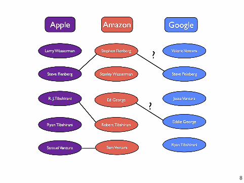
Record linkage

Record linkage is the process of merging together noisy databasesto remove duplicate entries.

7

8

9

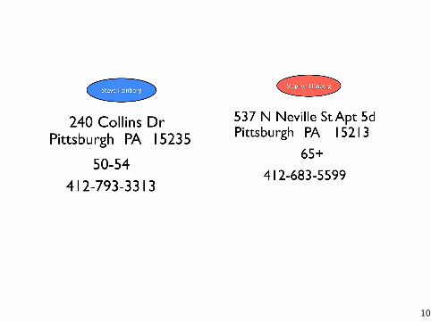
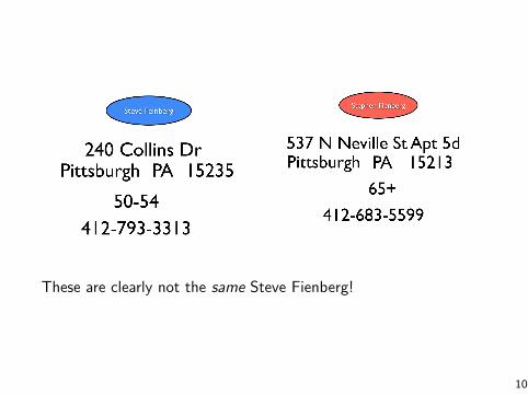
These are clearly not the same Steve Fienberg!

10

These are clearly not the same Steve Fienberg!

10

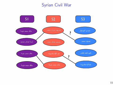
Syrian Civil War

11

Bayesian Model

I Define α`(w) = relative frequency of w in data for field `.

I G`: empirical distribution for field `.

I W ∼ F`(w0): P (W = w) ∝ α`(w) exp[−c d(w,w0)] , where d(·, ·)is a string metric and c > 0.

Xij` | λij , Yλij`, zij` ∼

δ(Yλij`) if zij` = 0

F`(Yλij`) if zij` = 1 and field ` is string-valued

G` if zij` = 1 and field ` is categorical

Yj′` ∼ G`zij` | βi` ∼ Bernoulli(βi`)

βi` ∼ Beta(a, b)

λij ∼ DiscreteUniform(1, . . . , Nmax), where Nmax =

k∑i=1

ni.

12

Bayesian Model

I Define α`(w) = relative frequency of w in data for field `.

I G`: empirical distribution for field `.

I W ∼ F`(w0): P (W = w) ∝ α`(w) exp[−c d(w,w0)] , where d(·, ·)is a string metric and c > 0.

Xij` | λij , Yλij`, zij` ∼

δ(Yλij`) if zij` = 0

F`(Yλij`) if zij` = 1 and field ` is string-valued

G` if zij` = 1 and field ` is categorical

Yj′` ∼ G`zij` | βi` ∼ Bernoulli(βi`)

βi` ∼ Beta(a, b)

λij ∼ DiscreteUniform(1, . . . , Nmax), where Nmax =

k∑i=1

ni.

12

Bayesian Model

I Define α`(w) = relative frequency of w in data for field `.

I G`: empirical distribution for field `.

I W ∼ F`(w0): P (W = w) ∝ α`(w) exp[−c d(w,w0)] , where d(·, ·)is a string metric and c > 0.

Xij` | λij , Yλij`, zij` ∼

δ(Yλij`) if zij` = 0

F`(Yλij`) if zij` = 1 and field ` is string-valued

G` if zij` = 1 and field ` is categorical

Yj′` ∼ G`zij` | βi` ∼ Bernoulli(βi`)

βi` ∼ Beta(a, b)

λij ∼ DiscreteUniform(1, . . . , Nmax), where Nmax =

k∑i=1

ni.

12

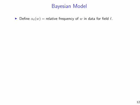
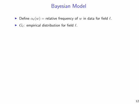
Bayesian Model

I Define α`(w) = relative frequency of w in data for field `.

I G`: empirical distribution for field `.

I W ∼ F`(w0): P (W = w) ∝ α`(w) exp[−c d(w,w0)] , where d(·, ·)is a string metric and c > 0.

Xij` | λij , Yλij`, zij` ∼

δ(Yλij`) if zij` = 0

F`(Yλij`) if zij` = 1 and field ` is string-valued

G` if zij` = 1 and field ` is categorical

Yj′` ∼ G`zij` | βi` ∼ Bernoulli(βi`)

βi` ∼ Beta(a, b)

λij ∼ DiscreteUniform(1, . . . , Nmax), where Nmax =

k∑i=1

ni.

12

The model I showed you is very complicated.

This course will give you an intro to Bayesian models and methods.

Often Bayesian models are hard to work with, so we’ll learn aboutapproximations.

The above record linkage problem is one that needs such anapproximation.

13

I “Bayesian” traces its origin to the 18th century and EnglishReverend Thomas Bayes, who along with Pierre-SimonLaplace discovered what we now call “Bayes’ Theorem”.

p(θ|x) =p(x|θ)p(θ)p(x)

∝ p(x|θ)p(θ). (1)

We can decompose Bayes’ Theorem into three principal terms:

p(θ|x) posterior

p(x|θ) likelihood

p(θ) prior

14

I “Bayesian” traces its origin to the 18th century and EnglishReverend Thomas Bayes, who along with Pierre-SimonLaplace discovered what we now call “Bayes’ Theorem”.

p(θ|x) =p(x|θ)p(θ)p(x)

∝ p(x|θ)p(θ). (1)

We can decompose Bayes’ Theorem into three principal terms:

p(θ|x) posterior

p(x|θ) likelihood

p(θ) prior

14

I “Bayesian” traces its origin to the 18th century and EnglishReverend Thomas Bayes, who along with Pierre-SimonLaplace discovered what we now call “Bayes’ Theorem”.

p(θ|x) =p(x|θ)p(θ)p(x)

∝ p(x|θ)p(θ). (1)

We can decompose Bayes’ Theorem into three principal terms:

p(θ|x) posterior

p(x|θ) likelihood

p(θ) prior

14

I “Bayesian” traces its origin to the 18th century and EnglishReverend Thomas Bayes, who along with Pierre-SimonLaplace discovered what we now call “Bayes’ Theorem”.

p(θ|x) =p(x|θ)p(θ)p(x)

∝ p(x|θ)p(θ). (1)

We can decompose Bayes’ Theorem into three principal terms:

p(θ|x) posterior

p(x|θ) likelihood

p(θ) prior

14

I “Bayesian” traces its origin to the 18th century and EnglishReverend Thomas Bayes, who along with Pierre-SimonLaplace discovered what we now call “Bayes’ Theorem”.

p(θ|x) =p(x|θ)p(θ)p(x)

∝ p(x|θ)p(θ). (1)

We can decompose Bayes’ Theorem into three principal terms:

p(θ|x) posterior

p(x|θ) likelihood

p(θ) prior

14

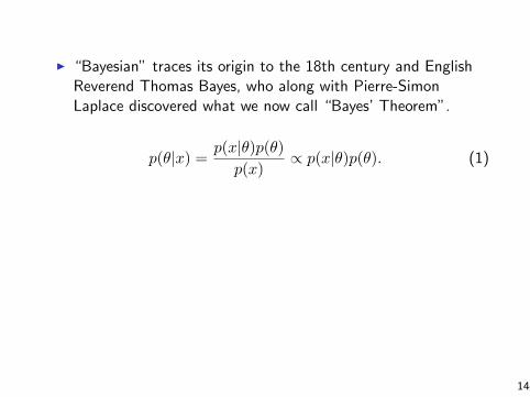
I “Bayesian” traces its origin to the 18th century and EnglishReverend Thomas Bayes, who along with Pierre-SimonLaplace discovered what we now call “Bayes’ Theorem”.

p(θ|x) =p(x|θ)p(θ)p(x)

∝ p(x|θ)p(θ). (1)

We can decompose Bayes’ Theorem into three principal terms:

p(θ|x) posterior

p(x|θ) likelihood

p(θ) prior

14

Polling Example 2012

Let’s apply this to a real example! We’re interested in theproportion of people that approve of President Obama in PA.

I We take a random sample of 10 people in PA and find that 6approve of President Obama.

I The national approval rating (Zogby poll) of President Obamain mid-December was 45%. We’ll assume that in PA hisapproval rating is approximately 50%.

I Based on this prior information, we’ll use a Beta prior for θand we’ll choose a and b. (Won’t get into this here).

I We can plot the prior and likelihood distributions in R andthen see how the two mix to form the posterior distribution.

15

Polling Example 2012

Let’s apply this to a real example! We’re interested in theproportion of people that approve of President Obama in PA.

I We take a random sample of 10 people in PA and find that 6approve of President Obama.

I The national approval rating (Zogby poll) of President Obamain mid-December was 45%. We’ll assume that in PA hisapproval rating is approximately 50%.

I Based on this prior information, we’ll use a Beta prior for θand we’ll choose a and b. (Won’t get into this here).

I We can plot the prior and likelihood distributions in R andthen see how the two mix to form the posterior distribution.

15

Polling Example 2012

Let’s apply this to a real example! We’re interested in theproportion of people that approve of President Obama in PA.

I We take a random sample of 10 people in PA and find that 6approve of President Obama.

I The national approval rating (Zogby poll) of President Obamain mid-December was 45%. We’ll assume that in PA hisapproval rating is approximately 50%.

I Based on this prior information, we’ll use a Beta prior for θand we’ll choose a and b. (Won’t get into this here).

I We can plot the prior and likelihood distributions in R andthen see how the two mix to form the posterior distribution.

15

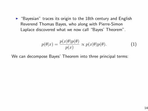
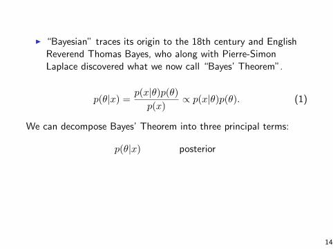
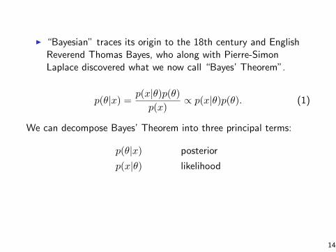
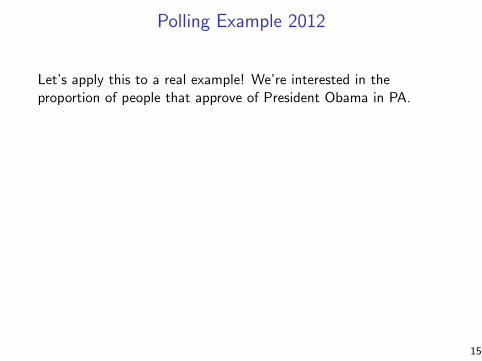
Polling Example 2012

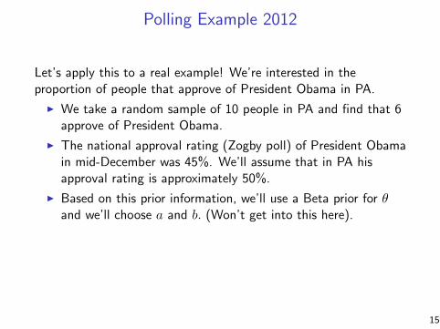
Let’s apply this to a real example! We’re interested in theproportion of people that approve of President Obama in PA.

I We take a random sample of 10 people in PA and find that 6approve of President Obama.

I The national approval rating (Zogby poll) of President Obamain mid-December was 45%. We’ll assume that in PA hisapproval rating is approximately 50%.

I Based on this prior information, we’ll use a Beta prior for θand we’ll choose a and b. (Won’t get into this here).

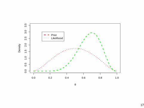
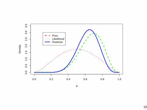
I We can plot the prior and likelihood distributions in R andthen see how the two mix to form the posterior distribution.

15

Polling Example 2012

Let’s apply this to a real example! We’re interested in theproportion of people that approve of President Obama in PA.

I We take a random sample of 10 people in PA and find that 6approve of President Obama.

I The national approval rating (Zogby poll) of President Obamain mid-December was 45%. We’ll assume that in PA hisapproval rating is approximately 50%.

I Based on this prior information, we’ll use a Beta prior for θand we’ll choose a and b. (Won’t get into this here).

I We can plot the prior and likelihood distributions in R andthen see how the two mix to form the posterior distribution.

15

0.0 0.2 0.4 0.6 0.8 1.0

0.0

0.5

1.0

1.5

2.0

2.5

3.0

3.5

θ

Den

sity

Prior

16

0.0 0.2 0.4 0.6 0.8 1.0

0.0

0.5

1.0

1.5

2.0

2.5

3.0

3.5

θ

Den

sity

PriorLikelihood

17

0.0 0.2 0.4 0.6 0.8 1.0

0.0

0.5

1.0

1.5

2.0

2.5

3.0

3.5

θ

Den

sity

PriorLikelihoodPosterior

18

The basic philosophical difference between the frequentist andBayesian paradigms is that

I Bayesians treat an unknown parameter θ as random.

I Frequentists treat θ as unknown but fixed.

19

The basic philosophical difference between the frequentist andBayesian paradigms is that

I Bayesians treat an unknown parameter θ as random.

I Frequentists treat θ as unknown but fixed.

19

Stopping Rule

Let θ be the probability of a particular coin landing on heads, andsuppose we want to test the hypotheses

H0 : θ = 1/2, H1 : θ > 1/2

at a significance level of α = 0.05. Suppose we observe thefollowing sequence of flips:

heads, heads, heads, heads, heads, tails (5 heads, 1 tails)

I To perform a frequentist hypothesis test, we must define arandom variable to describe the data.

I The proper way to do this depends on exactly which of thefollowing two experiments was actually performed:

20

Stopping Rule

Let θ be the probability of a particular coin landing on heads, andsuppose we want to test the hypotheses

H0 : θ = 1/2, H1 : θ > 1/2

at a significance level of α = 0.05. Suppose we observe thefollowing sequence of flips:

heads, heads, heads, heads, heads, tails (5 heads, 1 tails)

I To perform a frequentist hypothesis test, we must define arandom variable to describe the data.

I The proper way to do this depends on exactly which of thefollowing two experiments was actually performed:

20

Stopping Rule

Let θ be the probability of a particular coin landing on heads, andsuppose we want to test the hypotheses

H0 : θ = 1/2, H1 : θ > 1/2

at a significance level of α = 0.05. Suppose we observe thefollowing sequence of flips:

heads, heads, heads, heads, heads, tails (5 heads, 1 tails)

I To perform a frequentist hypothesis test, we must define arandom variable to describe the data.

I The proper way to do this depends on exactly which of thefollowing two experiments was actually performed:

20

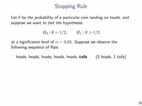
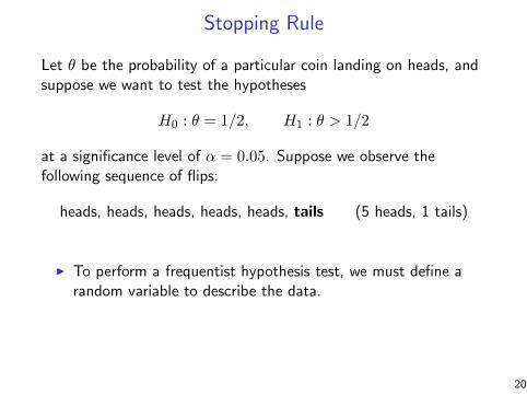
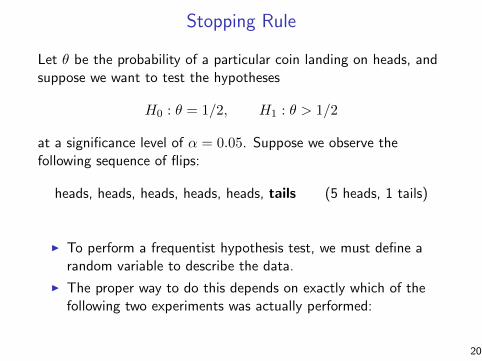
Stopping Rule

Let θ be the probability of a particular coin landing on heads, andsuppose we want to test the hypotheses

H0 : θ = 1/2, H1 : θ > 1/2

at a significance level of α = 0.05. Suppose we observe thefollowing sequence of flips:

heads, heads, heads, heads, heads, tails (5 heads, 1 tails)

I To perform a frequentist hypothesis test, we must define arandom variable to describe the data.

I The proper way to do this depends on exactly which of thefollowing two experiments was actually performed:

20

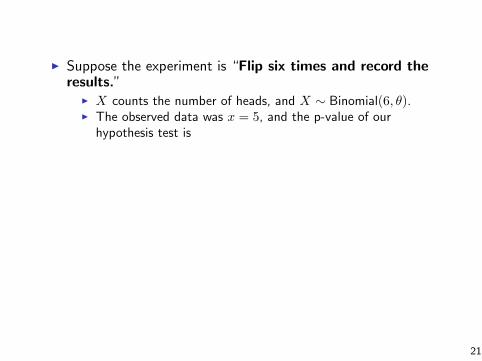
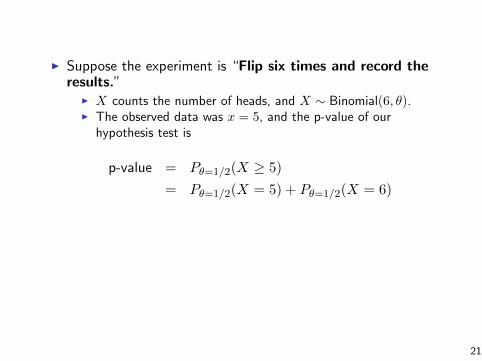
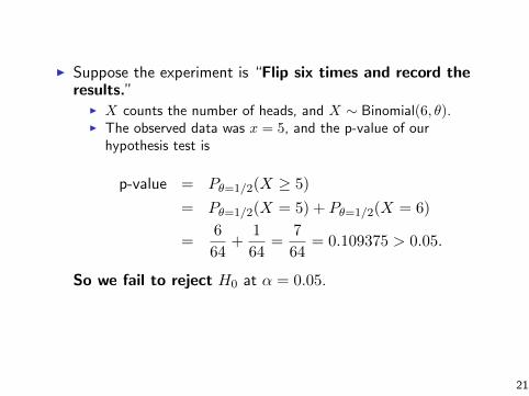
I Suppose the experiment is “Flip six times and record theresults.”

I X counts the number of heads, and X ∼ Binomial(6, θ).I The observed data was x = 5, and the p-value of our

hypothesis test is

p-value = Pθ=1/2(X ≥ 5)

= Pθ=1/2(X = 5) + Pθ=1/2(X = 6)

=6

64+

1

64=

7

64= 0.109375 > 0.05.

So we fail to reject H0 at α = 0.05.

21

I Suppose the experiment is “Flip six times and record theresults.”

I X counts the number of heads, and X ∼ Binomial(6, θ).I The observed data was x = 5, and the p-value of our

hypothesis test is

p-value = Pθ=1/2(X ≥ 5)

= Pθ=1/2(X = 5) + Pθ=1/2(X = 6)

=6

64+

1

64=

7

64= 0.109375 > 0.05.

So we fail to reject H0 at α = 0.05.

21

I Suppose the experiment is “Flip six times and record theresults.”

I X counts the number of heads, and X ∼ Binomial(6, θ).I The observed data was x = 5, and the p-value of our

hypothesis test is

p-value = Pθ=1/2(X ≥ 5)

= Pθ=1/2(X = 5) + Pθ=1/2(X = 6)

=6

64+

1

64=

7

64= 0.109375 > 0.05.

So we fail to reject H0 at α = 0.05.

21

I Suppose the experiment is “Flip six times and record theresults.”

I X counts the number of heads, and X ∼ Binomial(6, θ).I The observed data was x = 5, and the p-value of our

hypothesis test is

p-value = Pθ=1/2(X ≥ 5)

= Pθ=1/2(X = 5) + Pθ=1/2(X = 6)

=6

64+

1

64=

7

64= 0.109375 > 0.05.

So we fail to reject H0 at α = 0.05.

21

I Suppose the experiment is “Flip six times and record theresults.”

I X counts the number of heads, and X ∼ Binomial(6, θ).I The observed data was x = 5, and the p-value of our

hypothesis test is

p-value = Pθ=1/2(X ≥ 5)

= Pθ=1/2(X = 5) + Pθ=1/2(X = 6)

=6

64+

1

64=

7

64= 0.109375 > 0.05.

So we fail to reject H0 at α = 0.05.

21

I Suppose now the experiment is “Flip until we get tails.”

I X counts the number of the flip on which the first tails occurs,and X ∼ Geometric(1− θ).

I The observed data was x = 6, and the p-value of ourhypothesis test is

p-value = Pθ=1/2(X ≥ 6)

= 1− Pθ=1/2(X < 6)

= 1−5∑

x=1

Pθ=1/2(X = x)

= 1−(

1

2+

1

4+

1

8+

1

16+

1

32

)=

1

32= 0.03125 < 0.05.

So we reject H0 at α = 0.05.

22

I Suppose now the experiment is “Flip until we get tails.”

I X counts the number of the flip on which the first tails occurs,and X ∼ Geometric(1− θ).

I The observed data was x = 6, and the p-value of ourhypothesis test is

p-value = Pθ=1/2(X ≥ 6)

= 1− Pθ=1/2(X < 6)

= 1−5∑

x=1

Pθ=1/2(X = x)

= 1−(

1

2+

1

4+

1

8+

1

16+

1

32

)=

1

32= 0.03125 < 0.05.

So we reject H0 at α = 0.05.

22

I Suppose now the experiment is “Flip until we get tails.”

I X counts the number of the flip on which the first tails occurs,and X ∼ Geometric(1− θ).

I The observed data was x = 6, and the p-value of ourhypothesis test is

p-value = Pθ=1/2(X ≥ 6)

= 1− Pθ=1/2(X < 6)

= 1−5∑

x=1

Pθ=1/2(X = x)

= 1−(

1

2+

1

4+

1

8+

1

16+

1

32

)=

1

32= 0.03125 < 0.05.

So we reject H0 at α = 0.05.

22

I Suppose now the experiment is “Flip until we get tails.”

I X counts the number of the flip on which the first tails occurs,and X ∼ Geometric(1− θ).

I The observed data was x = 6, and the p-value of ourhypothesis test is

p-value = Pθ=1/2(X ≥ 6)

= 1− Pθ=1/2(X < 6)

= 1−5∑

x=1

Pθ=1/2(X = x)

= 1−(

1

2+

1

4+

1

8+

1

16+

1

32

)=

1

32= 0.03125 < 0.05.

So we reject H0 at α = 0.05.

22

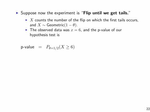
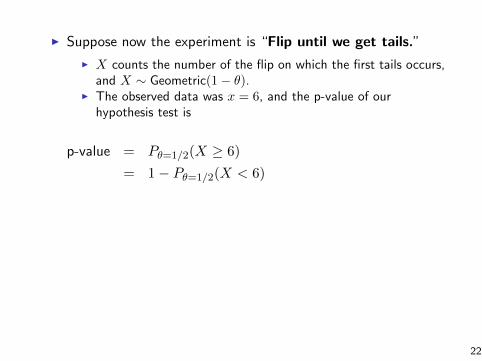
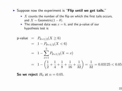
I Suppose now the experiment is “Flip until we get tails.”

I X counts the number of the flip on which the first tails occurs,and X ∼ Geometric(1− θ).

I The observed data was x = 6, and the p-value of ourhypothesis test is

p-value = Pθ=1/2(X ≥ 6)

= 1− Pθ=1/2(X < 6)

= 1−5∑

x=1

Pθ=1/2(X = x)

= 1−(

1

2+

1

4+

1

8+

1

16+

1

32

)=

1

32= 0.03125 < 0.05.

So we reject H0 at α = 0.05.

22

I The conclusions differ, which seems strikes some people asabsurd.

I P-values aren’t close—one is 3.5 times as large as the other.

I The result our hypothesis test depends on whether we wouldhave stopped flipping if we had gotten a tails sooner.

I The tests are dependent on what we call the stopping rule.

23

I The conclusions differ, which seems strikes some people asabsurd.

I P-values aren’t close—one is 3.5 times as large as the other.

I The result our hypothesis test depends on whether we wouldhave stopped flipping if we had gotten a tails sooner.

I The tests are dependent on what we call the stopping rule.

23

I The conclusions differ, which seems strikes some people asabsurd.

I P-values aren’t close—one is 3.5 times as large as the other.

I The result our hypothesis test depends on whether we wouldhave stopped flipping if we had gotten a tails sooner.

I The tests are dependent on what we call the stopping rule.

23

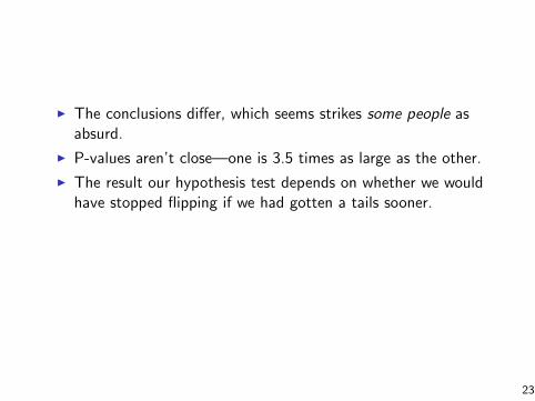
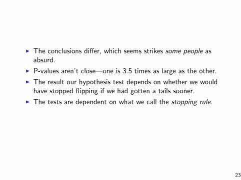
I The conclusions differ, which seems strikes some people asabsurd.

I P-values aren’t close—one is 3.5 times as large as the other.

I The result our hypothesis test depends on whether we wouldhave stopped flipping if we had gotten a tails sooner.

I The tests are dependent on what we call the stopping rule.

23

I The likelihood for the actual value of x that was observed isthe same for both experiments (up to a constant):

p(x|θ) ∝ θ5(1− θ).

I A Bayesian approach would take the data into account onlythrough this likelihood.

I This would provide the same answers regardless of whichexperiment was being performed.

The Bayesian analysis is independent of the stopping rule since itonly depends on the likelihood (show this at home!).

24

I The likelihood for the actual value of x that was observed isthe same for both experiments (up to a constant):

p(x|θ) ∝ θ5(1− θ).

I A Bayesian approach would take the data into account onlythrough this likelihood.

I This would provide the same answers regardless of whichexperiment was being performed.

The Bayesian analysis is independent of the stopping rule since itonly depends on the likelihood (show this at home!).

24

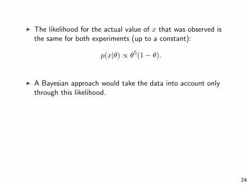
I The likelihood for the actual value of x that was observed isthe same for both experiments (up to a constant):

p(x|θ) ∝ θ5(1− θ).

I A Bayesian approach would take the data into account onlythrough this likelihood.

I This would provide the same answers regardless of whichexperiment was being performed.

The Bayesian analysis is independent of the stopping rule since itonly depends on the likelihood (show this at home!).

24

Hierarchical Bayesian Models

In a hierarchical Bayesian model, rather than specifying the priordistribution as a single function, we specify it as a hierarchy.

25

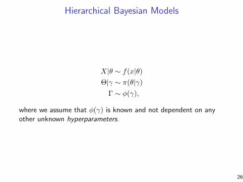
Hierarchical Bayesian Models

X|θ ∼ f(x|θ)Θ|γ ∼ π(θ|γ)

Γ ∼ φ(γ),

where we assume that φ(γ) is known and not dependent on anyother unknown hyperparameters.

26

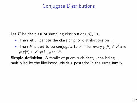
Conjugate Distributions

Let F be the class of sampling distributions p(y|θ).

I Then let P denote the class of prior distributions on θ.

I Then P is said to be conjugate to F if for every p(θ) ∈ P andp(y|θ) ∈ F, p(θ | y) ∈ P.

Simple definition: A family of priors such that, upon beingmultiplied by the likelihood, yields a posterior in the same family.

27

Conjugate Distributions

Let F be the class of sampling distributions p(y|θ).I Then let P denote the class of prior distributions on θ.

I Then P is said to be conjugate to F if for every p(θ) ∈ P andp(y|θ) ∈ F, p(θ | y) ∈ P.

Simple definition: A family of priors such that, upon beingmultiplied by the likelihood, yields a posterior in the same family.

27

Conjugate Distributions

Let F be the class of sampling distributions p(y|θ).I Then let P denote the class of prior distributions on θ.

I Then P is said to be conjugate to F if for every p(θ) ∈ P andp(y|θ) ∈ F, p(θ | y) ∈ P.

Simple definition: A family of priors such that, upon beingmultiplied by the likelihood, yields a posterior in the same family.

27

Beta-Binomial

If X|θ is distributed as binomial(n, θ), then a conjugate prior is thebeta family of distributions, where we can show that the posterioris

π(θ|x) ∝ p(x|θ)p(θ)

∝(n

x

)θx(1− θ)n−x Γ(a+ b)

Γ(a)Γ(b)θa−1(1− θ)b−1

∝ θx(1− θ)n−xθa−1(1− θ)b−1

∝ θx+a−1(1− θ)n−x+b−1 =⇒

θ|x ∼ Beta(x+ a, n− x+ b).

28

Beta-Binomial

If X|θ is distributed as binomial(n, θ), then a conjugate prior is thebeta family of distributions, where we can show that the posterioris

π(θ|x) ∝ p(x|θ)p(θ)

∝(n

x

)θx(1− θ)n−x Γ(a+ b)

Γ(a)Γ(b)θa−1(1− θ)b−1

∝ θx(1− θ)n−xθa−1(1− θ)b−1

∝ θx+a−1(1− θ)n−x+b−1 =⇒

θ|x ∼ Beta(x+ a, n− x+ b).

28

Beta-Binomial

If X|θ is distributed as binomial(n, θ), then a conjugate prior is thebeta family of distributions, where we can show that the posterioris

π(θ|x) ∝ p(x|θ)p(θ)

∝(n

x

)θx(1− θ)n−x Γ(a+ b)

Γ(a)Γ(b)θa−1(1− θ)b−1

∝ θx(1− θ)n−xθa−1(1− θ)b−1

∝ θx+a−1(1− θ)n−x+b−1 =⇒

θ|x ∼ Beta(x+ a, n− x+ b).

28

Beta-Binomial

If X|θ is distributed as binomial(n, θ), then a conjugate prior is thebeta family of distributions, where we can show that the posterioris

π(θ|x) ∝ p(x|θ)p(θ)

∝(n

x

)θx(1− θ)n−x Γ(a+ b)

Γ(a)Γ(b)θa−1(1− θ)b−1

∝ θx(1− θ)n−xθa−1(1− θ)b−1

∝ θx+a−1(1− θ)n−x+b−1 =⇒

θ|x ∼ Beta(x+ a, n− x+ b).

28

Beta-Binomial

If X|θ is distributed as binomial(n, θ), then a conjugate prior is thebeta family of distributions, where we can show that the posterioris

π(θ|x) ∝ p(x|θ)p(θ)

∝(n

x

)θx(1− θ)n−x Γ(a+ b)

Γ(a)Γ(b)θa−1(1− θ)b−1

∝ θx(1− θ)n−xθa−1(1− θ)b−1

∝ θx+a−1(1− θ)n−x+b−1 =⇒

θ|x ∼ Beta(x+ a, n− x+ b).

28

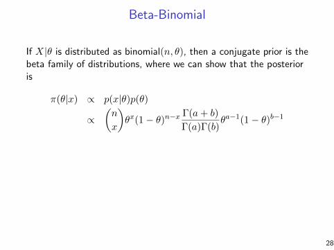
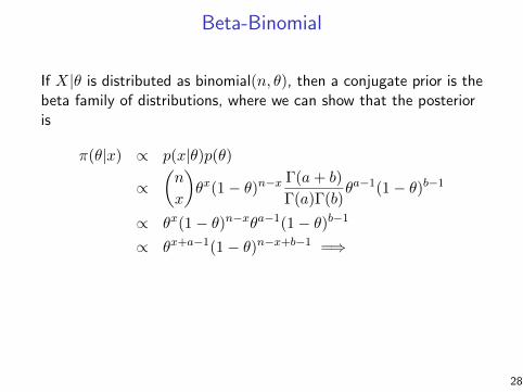
Beta-Binomial

If X|θ is distributed as binomial(n, θ), then a conjugate prior is thebeta family of distributions, where we can show that the posterioris

π(θ|x) ∝ p(x|θ)p(θ)

∝(n

x

)θx(1− θ)n−x Γ(a+ b)

Γ(a)Γ(b)θa−1(1− θ)b−1

∝ θx(1− θ)n−xθa−1(1− θ)b−1

∝ θx+a−1(1− θ)n−x+b−1 =⇒

θ|x ∼ Beta(x+ a, n− x+ b).

28