Intraday high-frequency FX trading with adaptive neuro ... · PDF fileIntraday high-frequency FX trading with ANFISs 69 studied (Murphy, 1986). This paper presents a model that tries

68 Int. J. Financial Markets and Derivatives, Vol. 2, Nos. 1/2, 2011

Copyright © 2011 Inderscience Enterprises Ltd.

Intraday high-frequency FX trading with adaptive neuro-fuzzy inference systems

Abdalla Kablan* and Wing Lon Ng Centre for Computational Finance and Economic Agents (CCFEA), University of Essex, Wivenhoe Park, Colchester, CO4 3SQ, UK E-mail: [email protected] E-mail: [email protected] *Corresponding author

Abstract: This paper introduces an adaptive neuro-fuzzy inference system (ANFIS) for financial trading, which learns to predict price movements from training data consisting of intraday tick data sampled at high frequency. The empirical data used in our investigation are five-minute mid-price time series from FX markets. The ANFIS optimisation involves back-testing as well as varying the number of epochs, and is combined with a new method of capturing volatility using an event-driven approach that takes into consideration directional changes within pre-specified thresholds. The results show that the proposed model outperforms standard strategies such as buy-and-hold or linear forecasting.

Keywords: high-frequency finance; trading; adaptive neuro-fuzzy inference system; ANFIS; foreign exchange markets; intraday seasonality.

Reference to this paper should be made as follows: Kablan, A. and Ng, W.L. (2011) ‘Intraday high-frequency FX trading with adaptive neuro-fuzzy inference systems’, Int. J. Financial Markets and Derivatives, Vol. 2, Nos. 1/2, pp.68–87.

Biographical notes: Abdalla Kablan’s research interests include artificial intelligence and its applications in financial engineering. His research also includes the applications of heuristics and neuro-fuzzy systems for financial decision making.

Wing Lon Ng is a Lecturer in High-Frequency Finance. His research interests include financial econometrics and computational finance and their applications in empirical market microstructure analysis.

1 Introduction

Financial investors and traders have always attempted to forecast the movement of stock markets (e.g., Schulmeister, 2009). Financial trading itself is embedded in a complex structure not only involving the dynamics of price formation but also the market microstructure itself. Market information, news and external factors affect the investors’ trading decisions concerning buying and selling. Usually, the price pattern is hard to recognise, notice or categorise, regardless of the type of the actual financial market

Intraday high-frequency FX trading with ANFISs 69

studied (Murphy, 1986). This paper presents a model that tries to prove that artificial intelligence and soft computing such as the adaptive neuro-fuzzy inference system (ANFIS) can provide a major solution in such tasks. The fuzzy logic approach, inspired by a model of human reasoning in which linguistic terms are used and fuzzy (as opposed to crisp) quantities are manipulated, is combined in neuro-fuzzy systems with the pattern recognition ability of neural networks (see Konstantaras et al., 2006; Sewell, 2010).

The recent escalation in computing power has led to a vast increase in the availability of data and information. Computers, sensors and information channels are developing faster, and data is easier to collect than ever before. Due to the availability of real-time order book information nowadays, the difference in decision making and risk taking among various traders represents a complicated process that affects market conditions. High-frequency trading is a new discipline in financial trading where trends are analysed in tick-by-tick fashion and buy and sell decisions are consequently taken. Therefore, implementing a system that would provide a means of capturing and forecasting the market movements on the real-time level would help to improve an investor’s financial trading record (see Dacarogna et al., 2001; Dempster and Jones, 2001). This paper proposes a new computational processing and filtration technique that has not yet been fully discussed or implemented in the existing literature [for a recent survey on algorithmic trading strategies and trading systems, see Aldridge (2009), Schulmeister (2009), Yeh et al. (2011), and the references therein].

Traditionally, most prediction algorithms presented in literature focus on data mining which is the integration of statistics, machine-learning paradigms and the analysis of dynamical systems (e.g., Hellstrom and Holmström, 1998; Kasabov and Song, 2002). Furthermore, given that financial time series are often very noisy, a filtering process should remove such noise from the signal (Sheen, 2005). An ANFIS architecture was chosen for this automated trading system as it shows very high performance in modelling non-linear functions and in identifying non-linear components (Denaï et al., 2007). The proposed financial ANFIS uses a hybrid learning algorithm and is able to construct a unique input-output mapping based on both human knowledge (fuzzy rules) and stipulation input-output data pairs (Castillo et al., 2006). It also has shown excellent results in predicting time series (see Jang, 1993; Kasabov and Song, 2002). In addition, since the trading system deals with intraday data, the data input to the system must be deseasonalised in a specific manner in order to separate the deterministic component in the times series as it otherwise would introduce spurious autocorrelation. The deseasonalisation is performed using a new event-based measure of volatility (Glattfelder et al., 2010).

The reminder of the paper is organised as follows. Section 2 introduces the methodology. Section 3 presents the empirical data and the results. Section 4 concludes.

2 Methodology

In the following, Section 2.1 first describes the design and architecture of the ANFIS originally introduced by Jang (1993). Section 2.2 then expands on the use of ANFIS for financial trading. Section 2.3 introduces an event-based measure of volatility to be fed into the ANFIS to capture the intraday seasonality and to optimise the trading schedule.

70 A. Kablan and W.L. Ng

2.1 The ANFIS framework

The ANFIS is an adaptive network of nodes and directional links with associated learning rules. The approach learns the rules and membership functions from the data (Takagi and Sugeno, 1985). It is called adaptive because some or all of the nodes have parameters that affect the output of the node. These networks identify and learn relationships between inputs and outputs, and have high learning capability and membership function definition properties. Although adaptive networks cover a number of different approaches, for our purposes, we will conduct a detailed investigation of the method proposed by Jang et al. (1997) with the architecture shown in Figure 1.

Figure 1 ANFIS architecture for a two rule Sugeno system (see online version for colours)

1w

2w

11fw

22fw2w

1w

F

Y

X

A1

A2

B1

B2

∑

Layer 1 Layer 2 Layer 3 Layer 4 Layer 5

The circular nodes have a fixed input-output relation, whereas the square nodes have parameters to be learnt. Typical fuzzy rules are defined as a conditional statement in the form:

1 1 , .If X is A then Y is B (1)

2 2 , .If X is A then Y is B (2)

X and Y are linguistic variables; Ai and Bi are linguistic values determined by fuzzy sets on the particular universes of discourse X and Y respectively. However, in ANFIS we use the first order Takagi-Sugeno system (Takagi and Sugeno, 1985), which is:

1 1 1 1 1 1 , .If X is A and Y is B then f p X q Y r= + + (3)

2 2 2 2 2 2 , .If X is A and Y is B then f p X q Y r= + + (4)

X and Y represent the universes of discourse; Ai and Bi are linguistic terms defined by their membership functions, and pi, qi and ri are the consequent parameters that are updated in the forward pass in the learning algorithm. The forward pass propagates the input vector through the network layer by layer. In the backward pass, the error is returned through the network in a similar manner to back-propagation. We briefly discuss the five layers in the following:


1 The output of each node in Layer 1 is:

2

1,

1,

( ) 1, 2

( ) 3, 4.i

i

i A

i B

O x for i

O x for i

μ

μ−

= =

= = (5)

Hence, O1,i(x) is essentially the membership grade for x and y. Although the membership functions could be very flexible, experimental results lead to the conclusion that for the task of financial data training, the bell-shaped membership function is most appropriate (see, e.g., Abonyi et al., 2001). We calculate

21( ) ,

1i

A bi

i

xx c

a

μ =−

+

(6)

where ai, bi, and ci are parameters to be learnt. These are the premise parameters.

2 In Layer 2, every node is fixed. This is where the t-norm is used to ‘AND’ the membership grades, for example, the product:

2, ( ) ( ), 1, 2.i ii i A BO w x y iμ μ= = = (7)

3 Layer 3 contains fixed nodes that calculate the ratio of the firing strengths of the rules:

3,1 2

.ii i

wO w

w w= =

+ (8)

4 The nodes in Layer 4 are adaptive and perform the consequent of the rules:

( )4, .i i i i i i iO w f w p x q y r= = + + (9)

The parameters (pi, qi, ri) in this layer are to be determined and are referred to as the consequent parameters.

5 In Layer 5, a single node computes the overall output:

5, .i i ii i i

i ii

w fO w f

w∑

= =∑∑ (10)

This is how the input vector is typically fed through the network layer by layer. We then consider how the ANFIS learns the premise and consequent parameters for the membership functions and the rules. We apply the hybrid learning algorithm proposed by Jang et al. (1997) which uses a combination of steepest descent and least-squares estimation (LSE) to calibrate the parameters in the adaptive network (see also Fontenla-Romero et al., 2003). We split the total parameter set S into two further sets S1, the set of premise (non-linear) parameters, and S2, the set of consequent (linear) parameters. In this study, ANFIS uses a two-pass learning algorithm. In the forward pass, S1 is unmodified and S2 is computed using a LSE algorithm, whereas in the backward pass, S1 is unmodified and S2 is updated using a gradient descent algorithm such as back-propagation (see also illustration in Figure 2).


Figure 2 Learning algorithm forward and backward passes (see online version for colours)

The task of the ANFIS learning algorithm for this architecture is to tune all of the modifiable parameters, namely {ai, bi, ci} and {pi, qi, ri} to make the ANFIS output match the training data. When the premise parameters ai, bi, and ci of the membership function are fixed, the output of the ANFIS model can be written as

1 21 2 1 1 2 2

1 2 1 2.

w wf f f w f w f

w w w w= = +

+ + (11)

In particular, the learning process consists of a forward pass and back-propagation, where in the forward pass, functional signals go forward until Layer 4, and the consequent parameters are identified by the least-square estimate. In the backward pass, the error rates propagate backwards and the premise parameters are updated by the gradient descent.

For given fixed values of S1, the parameters in S2 found by this approach are guaranteed to be the global optimum. Table 1 provides a summary of the learning methods. The output error is used to adapt the premise parameters by means of a standard back-propagation algorithm. Table 1 Summary of different learning methods

Forward pass Backward pass

Premise parameters Fixed Gradient descent Consequent parameters LSE Fixed Signals Node o/p Error rates

There are four methods used to update the parameters, these are:

1 Gradient descent (GD) only: all parameters are updated by gradient descent.

2 GD and one pass of LSE: LSE is applied only once at the start so as to obtain the initial values of the consequent parameters. GD then updates.

3 GD and LSE: the proposed hybrid rule (see also Jang, 1993).

4 Sequential LSE only: uses a Kalman filter to update the parameters.

In this chapter, for the purpose of using ANFIS for financial predictions, we use the third entry from the above list as this method usually represents a good compromise between computational complexity and resulting performance (see also Mitra et al., 2008).


2.2 ANFIS for financial predictions and trading

The proposed system as described above now takes the price series as input; it first takes a certain amount of m data points for training and generating the initial fuzzy inference system from the data values, and then takes the next m data points for validation. This will generate an ANFIS that has modified its parameters and membership functions and is ready to produce a prediction for the next data points, given the pattern that it has recognised. The success rate of such a system would be determined by its level of accuracy in predicting the movement of the next trading periods in seconds, minutes, hours, days, weeks or months, depending on the trading frequency. Taking the correct decisions after processing all of the inputs from other blocks is also essential to a successful system (Sheen, 2005).

In particular, the system considers the past three price observations in the market x(t – 3), x(t – 2), x(t – 1) and the current observation x(t) in order to predict the next price observation x(t + 1) using ANFIS. This is then used as a movement indicator (either up or down). In other words, to make a prediction for t + 1, the system will be fed the current price at time t plus the previous three price observations t – 1, t – 2 and t – 3, respectively. Now that a system to ‘predict’ the movement of the market has been implemented, a suitable position can be opened according to the indicator of this prediction. The pseudo-code is shown in Figure 3.

Figure 3 Introducing the hold position when prediction does not change direction

BEGIN

Train the system using the last 500 points;

check the systems accuracy using the last 500 points;

REPEAT

from now till the next 100 points;

generate prediction;

if prediction is up -> then buy

if next prediction is up -> then hold

else if prediction is down -> then sell

if next prediction is down -> then hold

END

retrain;

Figure 4 illustrates the above described strategy, where hold positions are introduced and the buy sell frequency is reduced. When the red line goes down (dummy value = 0), the system is in sell mode, remaining unchanged means that it is in hold mode, and moving back up (dummy value = 1) means that it went to buy mode. Additionally, in order to increase the return of the trading investment, a final prediction and trading strategy was introduced where a ‘trigger pointer’ value is used. Therefore, for a sequence of buy and hold positions, if the prediction of the next time sample falls below the set trigger, the position is closed; hence, a sell position is opened. The trigger pointer value is updated


after each iteration, as illustrated in the pseudo code in Figure 5. Initially this trigger is set to the first value in the dataset.

Figure 4 Positions being placed according to the prediction of the movement (see online version for colours)

Figure 5 Introducing the trigger to track the prediction and detect directional changes to adjust position

trigger = price (1)

if prediction is up and prediction > trigger

then trigger = prediction(now-1)

position = buy;

else if prediction is down and prediction < trigger

then trigger = prediction(now-1)

position = sell;

After the implementation of the above ANFIS system, further experiments had to be performed in order to optimise the results obtained from the above system. One important test that has been conducted involved varying the number of epochs and step sizes in each run on the system. In adaptive networks theory, an epoch is defined as a single pass through the entire dataset (each set of data is evaluated once). This means that the more epochs we have, the more evaluations we get. However, this also takes longer.

One epoch is one sweep through all of the records in the dataset. This does not mean that the more epochs we have, the better will be the results. Our experiments have proven


that a threshold exists at which point a system will reach saturation, and no matter how many epochs are used, the performance will not improve. In fact, a too large number of epochs would result in overtraining for the system, causing a decrease in performance (see Figure 6a and 6b). The initial setup included an 80-epoch system that took 18.4 seconds to execute during each run.1 Experiments for various numbers of epochs have been used, which in turn have caused a change in the learning rate that can be analysed in the panels in Figure 6. The step size is considered as a variable that is corrected after every fourth epoch, counting from the epoch in which the previous correction has been done. It is realised on the basis of the following rules:

1 if the error undergoes four consecutive reductions, then increase the step size by 10%

2 if the error successively goes through a combination of increases and decreases, then decrease the step size by 10%.

Finally another variable is allocated to store the last change, which stores the index of the epoch in which the variable step size has been previously changed.

In general, there is no conclusive theory to decide the number of epochs in neural networks literature. However, it is a general rule to avoid the problem of overfitting when increasing the number of epochs. Practically, it is observed that the higher the number of training epochs the better is the classification performance but this worsens the ability of the generalisation by the network hence the ability to correctly predict the future processing data not seen before. This is confirmed by the results in Table 2 in the empirical section below, hence we choose 80 as an optimal epoch size [for a brief discussion on the choice of epoch numbers, see also Yezioro et al. (2008) and Chelani and Hasan (2001)].

Figure 6 Error curves and step size update for various epochs: (a, b) 180 epochs (c, d) 100 epochs (e, f) 50 epochs (g, h) 10 epochs (see online version for colours)

0 50 100 150

3

3.5

4

4.5

Error Curves

epoch number

root

mea

n sq

uare

d er

ror

Training ErrorChecking Error

0 50 100 150 200

0

0.05

0.1

0.15

0.2

0.25

epoch number

step

siz

e

step size curve

(a) (b)

0 20 40 60 80 100

3

3.5

4

4.5

Error Curves

epoch number

root

mea

n sq

uare

d er

ror


0 20 40 60 80 1000

0.05

0.1

0.15

0.2

0.25

epoch number

step

siz

e

step size curve

(c) (d)


Figure 6 Error curves and step size update for various epochs: (a, b) 180 epochs (c, d) 100 epochs (e, f) 50 epochs (g, h) 10 epochs (continued) (see online version for colours)

0 10 20 30 40 50

3

3.5

4

4.5

Error Curves

epoch number

root

mea

n sq

uare

d er

ror


0 10 20 30 40 50

0.1

0.15

0.2

0.25

epoch number

step

siz

e

step size curve

(e) (f)

0 2 4 6 8 10

3

3.5

4

Error Curves

epoch number

root

mea

n sq

uare

d er

ror


0 2 4 6 8 10

0.1

0.105

0.11

0.115

0.12

0.125

epoch number

step

siz

e

step size curve

(g) (h)

2.3 Intraday seasonality

As trading activities are observed in real-time, common approaches to measure volatility such as the standard deviation can not be applied due to the inhomogeneous data structure of the time series. Therefore, an Intraday Seasonality Observation Model (ISOM) as an event-based concept to measure market activity will be used in this study as a proxy for volatility as it can map the times of day with their respective volatility. This is viewed from an event-based perspective, where each ‘directional change’ with a specific threshold is an event. The aim is to use the ISOM to filter and clean this data by pointing out periods of the day when the volatility has exceeded a certain range (number of events). The idea here is to take the number of observations per intraday sampling interval in order to produce a model that would estimate the number of average observations that occur for the targeted time of day window (see also Bauwens et al., 2005).

In financial trading, directional-change (dc) events are understood as price movements, where a total-price move between two extreme price levels, expressed as a relative price jump of threshold size dx(%), can be decomposed into a price reversion (i.e., the directional-change itself) and an overshoot sections (Glattfelder et al., 2010). The ISOM for a particular time of day t at a particular threshold dx is equal to the total number of directional change events that occurred at that time window tbin in the entire dataset:


( ) ( )1

,n

bin dayday

ISOM t dx N dc t t=

= ∈∑ (12)

where n is the total number of days in the dataset, and N(dc) is the number of directional changes (events). In its simple definition, the ISOM is a model that takes into consideration a certain threshold dx(%) and will observe the timings where the directional changes dc occur. It would iteratively and consecutively parse through the entire dataset of prices and save the observations into their respective time bins. This would ultimately give a horizon of seasonalities, pointing out the exact times of day when these observations were made. This indicates the times of day when the volatility was high or low. The idea is that the data will be viewed from a scaling law perspective of directional changes (events), where each up/down percentage change within a pre-specified threshold is observed, the time stamps and relative price are marked, and all data is iteratively stored in bins of time value, which will then be analysed further.

For illustration purpose, when applied with a dx = 0.05% change for 30 minutes windows for the foreign exchange (FX) pair EUR-USD observed from 04/04/2006 to 04/04/2008. The ISOM resulted in the seasonality pattern shown in Figure 7. The plot reveals that most of the directional change events occur between 12:00 and 14:00 GMT. This confirms the fact that these are the times when the announcements are made and the market’s reaction to these announcements takes place. It is also the time when the US markets open; hence, the volatility of the markets increases. Other times of high volatility occur between 7:00 and 8:00 GMT, which is usually the time before the European markets open.

Figure 7 ISOM for a threshold of dx = 0.5% price move observed every 30 minutes for the FX pair EUR/USD from 04/04/2006 to 04/04/2008 (see online version for colours)

The ISOM shows that when considering observations every 30 minutes, the period with the highest volatility is between 12:30 and 13:00 GMT, which is again the time when all of the announcements that were made at 12:00 have been absorbed by the markets and the traders have started to act on them. The period of highest trading activity occurs between 12:00 and 16:00 GMT, i.e., the times that include the announcements, the opening of the US markets until the close of the European markets. The above results have confirmed real-life events that are known to increase markets volatility. They can


also help the trader or the system to ignore the periods that experience a low number of events.

It must be noted that the ISOM can be applied to any threshold and any time frequency (daily, half daily, quarter daily, five minutes, etc.). We have taken a threshold of dx = 0.05% for the scope of this illustration; the concept can be applied freely to any threshold or time frequency (additional figures illustrating the intraday seasonality for other threshold values are shown in Figure 10 in the Appendix).

The next step is now to use ISOM to filter and clean this data by pointing out periods of the day when the volatility has exceeded a certain range (number of events). The ISOM model has been redesigned to cater to five-minute data instead of hourly or 30-minute data, as previously shown. We now have bins of five-minute data, and we will capture the directional changes as they occur within these bins, where the counter of events will increase according to the number of events and the number of times that the threshold has been exceeded. In this study, ANFIS was fed data from the times of day when the number of observations exceeded ten events. After being trained on data with higher volatility (stress training), ANFIS will perform prediction of a set of checking data. The pseudo-code is shown in Figure 8.

Figure 8 Optimising ANFIS with ISOM

Function Collect-ISOM-Times BEGIN for i = 2 to end(in-sample-data) calculate the percentage directional changes dc(i) = (price(i) - price(i-1) * 100)/ price(i-1) if abs(dc(i))> 0.05% save time bin observation (T) count number of observations for respective time bin (Tcount) Observations_Per_Day = Tcount/length(in-sample-data) if Observations_Per_Day > 5 Valid_ISOM_Time_Bin = T end if end if end for END Function Use-ISOM-for-Training-ANFIS BEGIN for k = 1 to end(out-of-sample data) if time = Valid_ISOM_Time_Bin train ANFIS perform predictions else proceed to next time bin end if end for END


3 Empirical data and results

The FX market is a 24-hour worldwide market with high liquidity and volatility, especially in the three major financial centres with international influence: New York, London and Tokyo. Volatility is highest during the early morning in New York time because exchanges in London and New York are open and simultaneously trading. Stylised facts such as gain-loss asymmetry and heavy tails are observed in FX return distributions (Bauwens et al., 2005). Commercial banks, corporate, funding and retail institutions from around the globe participate in FX trading. The price at the FX market is formed by buying and selling currencies to institutions, traders, exporters, importers, portfolio managers and tourists. Nowadays, orders are electronically matched via automated brokerage terminals. Yoon et al. (1994) state that approximately 85% of all FX trading occurs between market makers. This creates an opportunity for speculation.

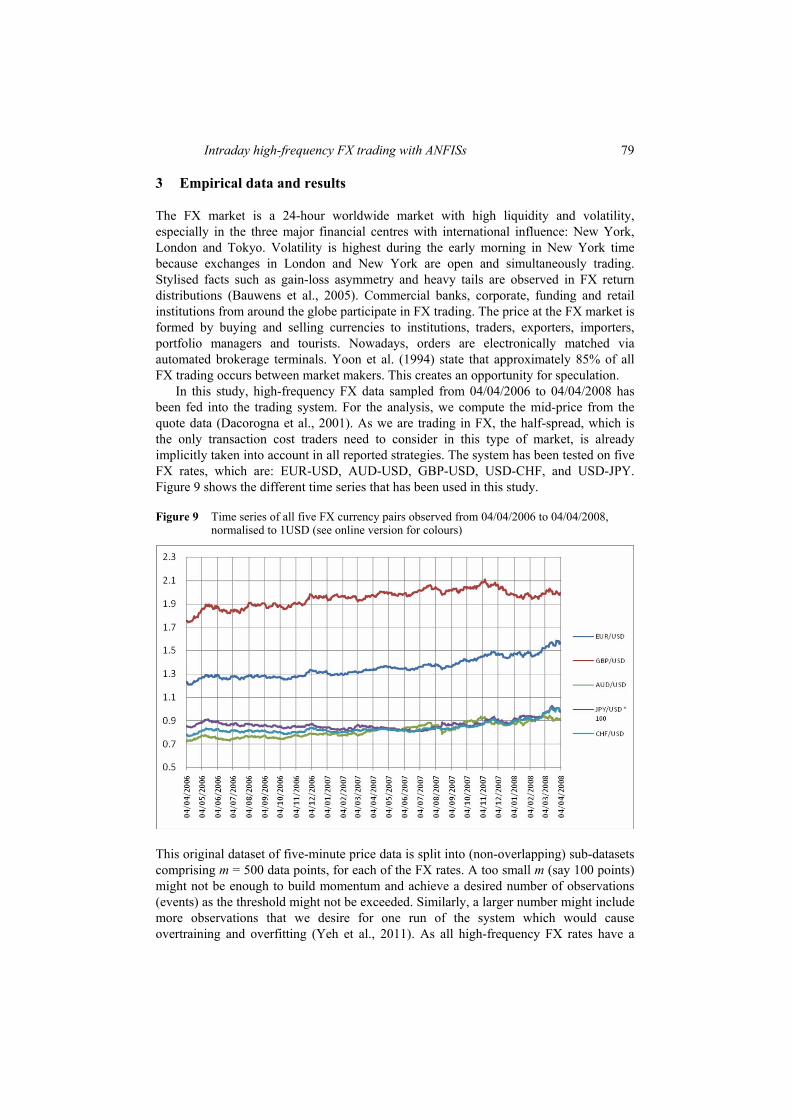
In this study, high-frequency FX data sampled from 04/04/2006 to 04/04/2008 has been fed into the trading system. For the analysis, we compute the mid-price from the quote data (Dacorogna et al., 2001). As we are trading in FX, the half-spread, which is the only transaction cost traders need to consider in this type of market, is already implicitly taken into account in all reported strategies. The system has been tested on five FX rates, which are: EUR-USD, AUD-USD, GBP-USD, USD-CHF, and USD-JPY. Figure 9 shows the different time series that has been used in this study.

Figure 9 Time series of all five FX currency pairs observed from 04/04/2006 to 04/04/2008, normalised to 1USD (see online version for colours)

This original dataset of five-minute price data is split into (non-overlapping) sub-datasets comprising m = 500 data points, for each of the FX rates. A too small m (say 100 points) might not be enough to build momentum and achieve a desired number of observations (events) as the threshold might not be exceeded. Similarly, a larger number might include more observations that we desire for one run of the system which would cause overtraining and overfitting (Yeh et al., 2011). As all high-frequency FX rates have a


different amount of data points, m was chosen such that the all series have reasonably comparable sub-datasets.

For each FX rates series, the first 500 ‘in-sample’ data points in each subset are used for system training. The subsequent 500 data points are considered as ‘out-of-sample’ and used for validating the system’s performance and updating the network structure using the output error. The 500 data points that were used for validation at one simulation can be reused for retraining the system in the next simulation, thus creating a rolling window approach for training and validating the system, making full use of all the available data.

In order to evaluate the performance of the proposed model, we will compare the ANFIS with the standard strategies that are commonly applied in the industry, such as buy and hold [e.g., Yeh et al., (2011), p.796, Section 2.2] or linear forecasting using trend following or trend reverting signals [e.g., Schulmeister (2009), pp.191–194, Section 2]. We use different measures for assessment, such as

a the wining rate

b the profit factor

c the return of investment (ROI)

d the Sharpe ratio

e the Sortino ratio.

The winning rate simply describes the number of winning trades against the overall number of trades. The profit factor mainly describes the historic profitability of a series of trades on an investment. The break-even of the profit factor is 1 meaning an investment that generates trades with a 50% chance of the gross sum of winning trades and a 50% chance of the gross sum of losing trades. Normally, investors pick investments with the profit factor higher than one. The ROI is used to evaluate the efficiency of an investment or compare returns on investments. That is, ROI is the ratio of profit gained or lost on an investment in relation to the amount of cost invested. The Sharpe ratio is used to the measure risk-adjusted return of an investment asset or a portfolio, which can tell investors how well the return of an asset compensates investors for the risk taken. The Sharpe ratio is defined as

,p f

p

R RSharpe ratio

σ−

=

where Rp denotes the expected return, Rf the risk-free interest rate and σp the portfolio volatility. Technically, this ratio measures the risk premium per each unit of total risk in an investment asset or a portfolio. Investors often pick investments with high Sharpe ratios because the higher the Sharpe ratio, the better its risk-adjusted performance has been. As there is no risk-free interest rate for intraday maturities, we use the mean return from the training sub-dataset as a substitute. Similarly, the Sortino ratio is defined as

,p f

neg

R RSortino ratio

σ−

=


where σneg denotes the standard deviation of only negative asset returns. The main difference between the Sharpe ratio and the Sortino ratio is that the Sortino ratio only penalises the downside volatility, while the Sharpe ratio penalises both upside and downside volatility. Thus, the Sortino ratio measures the risk premium per each unit of downside risk in an investment asset or a portfolio.

When training the ANFIS, it has been noticed after running initial experiments that the larger the numbers of epochs, the more stable the system will be because of damping oscillation (see Figure 6). Furthermore, the larger the size of the step, the faster the errors will decrease, although there will be more oscillations. When designing a system that will trade in high frequency, a major category that has to be satisfied along with high performance and optimum results is high speed or run-time and execution. As it can be seen from the Figure 6 and Table 2, a low (high) number of epochs results in a system that is rather fast (slow). On the other hand, a low number of epochs produces very poor results compared to a higher number of epochs, which produces a system with very high performance rates. However, it was also observed from the experiments that as the number of epochs increases, there may be a stage where the performance does not increase as much as required, whereas the time of execution increases drastically. Hence, it is a matter of compromise between speed and performance. This issue can be resolved by choosing a system with 80 epochs, where it has been found to produce the highest performance for the smallest amount of time after conducting extensive experiments (see Table 2). Furthermore, since the system trades on five-minute intervals, a time of 25.15 seconds cannot be considered a long execution time, given the complexity of the ANFIS design.

Having determined the number of epochs to be considered, ANFIS was fed data from the times of day when the number of observations exceeded ten events. After being trained on data with higher volatility (stress training), ANFIS will perform prediction of a set of checking data. Table 2 Out-of-sample evaluation of the ANFIS system using various numbers of epochs

Num. of epochs

CPU time (secs)

Winning rate

Profit factor ROI Sharpe

ratio Sortino ratio

10 3.72 0.40 1.9 0.07 0.13 0.12 50 12.53 0.55 2.1 0.15 0.14 0.19 80 25.15 0.65 2.3 0.27 0.19 0.20 100 28.31 0.65 2.3 0.27 0.19 0.21 180 50.27 0.64 2.4 0.26 0.18 0.20

As mentioned before, all sub-datasets used for validation of the implemented trading system is considered as the ‘out-of-sample’. The performance measures introduced above are computed for each validation sub-dataset. Table 3 reports the overall average performance measure for

1 the buy and hold

2 the momentum (trend following)

3 the contrarian (trend reversal)

4 the Intraday ANFIS trading strategy.


Table 3 Comparison of the average performance measures in the out-of-sample for all implemented trading strategies

FX pair Winning rate Profit factor ROI Sharpe ratio Sortino ratio

EUR-USD Buy and hold 0.42 1.1 0.09 –0.07 –0.05 Momentum 0.58 1.7 0.21 0.12 0.10 Contrarian 0.39 0.8 0.07 0.09 0.09 Intraday ANFIS 0.71 2.7 0.33 0.22 0.20 AUD-USD Buy and hold 0.51 0.9 0.11 0.03 0.01 Momentum 0.59 1.1 0.14 0.02 –0.02 Contrarian 0.53 1.2 0.18 –0.05 –0.06 Intraday ANFIS 0.56 1.4 0.17 0.01 –0.01 GBP-USD Buy and hold 0.51 1.3 0.11 0.04 0.05 Momentum 0.47 0.7 0.08 –0.01 –0.03 Contrarian 0.55 0.9 0.06 0.02 –0.02 Intraday ANFIS 0.50 0.9 0.07 –0.08 –0.09 USD-CHF Buy and hold 0.43 0.8 0.07 –0.02 –0.04 Momentum 0.57 1.3 0.10 0.09 0.04 Contrarian 0.54 1.0 0.12 0.07 –0.01 Intraday ANFIS 0.65 1.2 0.19 0.11 0.07 USD-JPY Buy and hold 0.29 0.4 0.01 –0.14 –0.17 Momentum 0.44 0.7 0.05 –0.02 –0.00 Contrarian 0.47 1.3 0.09 0.01 0.01 Intraday ANFIS 0.52 1.8 0.12 0.03 –0.01

With respect to the winning rate, Table 3 shows that in most cases, the ANFIS system outperforms the standard strategies in the overall number of wins. In terms of the profit factor, which indicates the actual profitability of a series of trades on an investment, the results show that the ANFIS system also has a profit factor higher than 1 in most cases. Table 3 also reveals that ANFIS generally obtains a higher ROI than the conventional strategies, i.e., it has a higher ratio of profit gained on a trade in relation to the amount of cost invested. Last not least, the Sharpe ratio and Sortino ratio, which measure the investment per unit of risk, also indicate a better performance of the ANFIS model, but less consistent as compared to the other benchmark values. Positive Sharpe and Sortino ratios imply that the trading strategy has not taken high risk.

Other descriptive statistics of performance measures in the ‘out-of-sample’ such as the standard deviation, skewness and kurtosis are listed in Table 4 in the Appendix. It can be seen that in general the performance measures for ANFIS have a lower standard deviation (higher accuracy), higher skewness (higher outperformance) as compared to the


benchmark models. Comparisons for the kurtosis are rather inconsistent, allowing no particular conclusion.

Finally, in order to statistically test the performance of a benchmark model (either buy and hold, momentum or contrarian) compared to the proposed ANFIS model, Table 5 in the Appendix lists the test-statistics of the (one tailed) t-test with the null-hypothesis that average measure for the benchmark is better than that for the ANFIS. A negative test-statistic with a value lower than –1.6649 indicates a rejection of the null-hypothesis at a 5% significance level, implying a statistically significant outperformance of the ANFIS strategy. Furthermore, a low positive value of the test-statistic would imply that a particular benchmark model is not significantly better than ANFIS (e.g., Sortino ratios for AUS-USD or USD-JPY).

4 Conclusions

The distinctive area of soft computing and artificial intelligence was addressed in this project by revisiting and improving the performance of the ANFIS by manipulating the number of epochs and the learning rate. It was concluded that a certain number of optimal epochs should not be exceeded, since this would not drastically improve the system. The ISOM proposed in this project has been tested on various threshold levels. The observation of a directional change within a threshold leads to taking the time stamp and its consequential addition to all of the observations that have been made during that time. The power of this method lies in the fact that any threshold can be used for any time frequency. This leads to the observation of events for the entire data series from a new perspective. The above concepts of event-driven volatility have proven to be consistent with ANFIS if sufficient data is present to perform the ISOM. A comparison of the proposed model against the standard trading strategies that are commonly applied in the industry shows an outperformance of the Intraday ANFIS.

Acknowledgements

The authors would like to thank Steve Phelps, Nikos S. Thomaidis (editor) and three anonymous referees for their valuable comments and suggestions that led to an improvement of this paper.

References Abonyi, J., Babuška, R., and Szeifert, F. (2001) ‘Fuzzy modeling with multivariate membership

functions: gray box identification and control design’, IEEE Transactions on Systems, Man, and Cybernetics – Part B, Vol. 31, No. 5, pp.755–767.

Aldridge, I. (2009) High-frequency Trading – A Practical Guide to Algorithmic Trading Strategies and Trading Systems, Wiley, NJ.

Bauwens, L., Omrane, B. and Giot, P. (2005) ‘News announcements, market activity and volatility in the euro-dollar foreign exchange market’, Journal of International Money and Finance, Vol. 24, No. 7, pp.1108–1125.


Castillo, E., Guijarro-Berdinas, B., Fontenla-Romero, O. and Alonso-Betanzos, A. (2006) ‘A very fast learning method for neural networks based on sensitivity analysis’, Journal of Machine Learning Research, Vol. 7, pp.1159–1182.

Chelani, A. and Hasan, M. (2001) ‘Forecasting nitrogene dioxide concentration in ambient air using artificial neural-networks’, International Journal of Environmental Studies, Vol. 58, No. 4, pp.487–499.

Dacarogna, M., Gençay, R., Müller, U.A., Pictet, O. and Olsen, R. (2001) An Introduction to High-Frequency Finance, Academic Press, San Diego.

Dempster, M.A.H. and Jones, C.M. (2001) ‘A real-time adaptive trading system using genetic programming’, Quantitative Finance, Vol. 1, No. 4, pp.397–413.

Denaï, M., Palis, F. and Zeghbib, A. (2007) ‘Modeling and control of non-linear systems using soft computing techniques’, Applied Soft Computing, Vol. 7, No. 3, pp.728–738.

Fontenla-Romero, O., Erdogomus, D., Principe, J.C., Alonso-Betanzos, A. and Castillo, E. (2003) ‘Linear least-squares based methods for neural networks learning’, Lecture Notes in Computer Science, Vol. 2714/2003, No. 173, pp.84–91.

Glattfelder, J.B., Dupuis, A. and Olsen, R. (2010) ‘Patterns in high-frequency FX data: discovery of 12 empirical scaling laws’, Working paper, arXiv:0809.1040v2.

Hellstrom, T. and Holmström, K. (1998) ‘Predicting the stock market’, Technical Report Ima-TOM-1997-07, Center of Mathematical Modeling, Department of Mathematics and Physics, Mälardalen University, Sweden.

Jang, J.R. (1993) ‘ANFIS: adaptive network-based fuzzy inference system’, IEEE Transactions on Systems, Man and Cybernetics, Vol. 23, No. 3, pp.665–685.

Jang, J.R., Sun, C.T. and Mizutani, E. (1997) Neuro-Fuzzy and Soft Computing, Prentice Hall, Upper Saddle River, NJ.

Kasabov, N.K. and Song, Q. (2002) ‘DENFIS: dynamic evolving neural-fuzzy inference system and its application for time-series prediction’, IEEE Transactions on Fuzzy Systems, Vol. 10, No. 2, pp.1–37.

Konstantaras, A., Varley, M.R., Vallianatos, F., Collins, G. and Holifield, P. (2006) ‘Neuro-fuzzy prediction-based adaptive filtering applied to severely distorted magnetic field recordings’, IEEE Geoscience and Remote Sensing Letters, Vol. 3, No. 4, pp.439–441.

Mitra, P., Maulik, S., Chowdhury, S.P. and Chowdhury, S. (2008) ‘ANFIS based automatic voltage regulator with hybrid learning algorithm’, International Journal of Innovations in Energy Systems and Power, Vol. 3, No. 2, pp.1–5.

Murphy, J. (1986) Technical Analysis of Futures Markets, New York Institute of Finance, New York.

Schulmeister, S. (2009) ‘Profitability of technical stock trading: has it moved from daily to intraday data?’, Review of Financial Economics, Vol. 18, No. 4, pp.190–201.

Sewell, M.V. (2010) ‘The application of intelligent systems to financial time series analysis’, PhD dissertation, Department of Computer Science, University College London, University of London.

Sheen, J.N. (2005) ‘Fuzzy financial decision-making: load management programs case study’, IEEE Transactions on Power Systems, Vol. 20, No. 4, pp.1808–1817.

Takagi, T. and Sugeno, M. (1985) ‘Fuzzy identification of systems and its application to modeling and control’, IEEE Transactions on Systems, Man and Cybernetics, Vol. 15, No. 1, pp.116–132.

Yeh, I-C., Lien, C. and Tsai, Y-C. (2011) ‘Evaluation approach to stock trading system using evolutionary computation’, Expert Systems with Applications, Vol. 38, No. 1, pp.794–803.

Yezioro, A., Dong, B. and Leite, F. (2008) ‘An applied artificial intelligence approach towards assessing building performance simulation tools’, Energy and Buildings, Vol. 40, No. 4, pp.612–620.


Yoon, Y., Guimaraes, T. and Swales, G. (1994) ‘Integrating artificial neural networks with rule-based expert systems’, Decision Support Systems, Vol. 11, No. 5, pp.497–507.

Notes 1 Simulations have been performed on a Toshiba Tecra A9-11M Laptop PC. CPU type: Intel

Core 2 Duo, CPU speed: 2.4 GHz, internal memory: 2048 MB, hard drive size: 160.0 GB.

Appendix

Figure 10 ISOM for alternative thresholds: (a) threshold = 0.2% (b) threshold = 0.4% (c) threshold = 0.6% (see online version for colours)

(a)

(b)

(c)


Table 4 Descriptive statistics for the performance measures in the out-of-sample for all implemented trading strategies


Table 5 t-tests on significance of the outperformance of the Intraday ANFIS compared to the benchmark models

Winning rate Profit factor ROI Sharpe ratio Sortino ratio

EUR-USD Buy and hold –25.1390 –87.7696 –9.1041 –5.6101 –8.0404 Momentum –25.2152 –44.1580 –9.9627 –5.0338 –3.3665 Contrarian –44.1665 –67.5499 –17.5153 –4.7709 –2.5080 AUD-USD Buy and hold –5.8162 –83.9129 –4.3898 –0.8362 0.9140 Momentum 6.5559 –41.3212 –4.3607 –0.5586 –0.3871 Contrarian –9.9370 –61.0892 1.0640 –5.0704 –1.5031 GBP-USD Buy and hold 0.6132 46.9026 1.9547 5.7761 5.6225 Momentum –4.2883 –75.8641 –0.7037 3.0029 3.5683 Contrarian 11.2452 1.9371 –1.4116 2.2437 2.5437 USD-CHF Buy and hold –18.3256 –32.8665 –8.4406 –3.5630 –7.4428 Momentum –49.3637 38.8532 –11.3662 –1.2525 –1.6518 Contrarian –32.5415 –50.9244 –9.7339 –2.1374 –7.0753 Intraday ANFIS –18.3256 –32.8665 –8.4406 –3.5630 –7.4428 USD-JPY Buy and hold –18.8390 –72.8580 –10.0507 –4.7790 –5.1781 Momentum –20.3472 –10.5751 –4.6689 –1.0293 0.3112 Contrarian –15.1101 –41.5113 –2.3427 –0.5362 0.5320

Notes: This table lists the test-statistics of the (one-tailed) t-test with the null-hypothesis that the average performance of a benchmark model (either buy and hold, momentum or contrarian) is better than that of the ANFIS model, i.e., H0: µBENCHMARK ≥ µANFIS. A negative value lower than –1.6649 indicates a rejection of the null at a 5% significance level.

Documents

Intraday high-frequency FX trading with adaptive neuro ... · PDF fileIntraday high-frequency FX trading with ANFISs 69 studied (Murphy, 1986). This paper presents a model that tries