Psychological Bulletin 1979, Vol. 86, No. 2, 420-428

I

Intraclass Correlations : Uses in Assessing Rater Reliability

Patrick E. Shrout and Joseph L. Fleiss Division of Biostatistics

Columbia University, School of Public Health

Reliability coefficients often take the form of intraclass correlation coefficients. In this article, guidelines are given for choosing among six different forms of the intraclass correlation for reliability studies in which n targets are rated by k judges. Relevant to the choice of the coefficient are the appropriate statistical model for the reliability study and the applications to be made of the reliability results. Confidence intervals for each of the forms are reviewed.

Most measurements in the behavioral sciences involve measurement error, but judgments made by humans are especially plagued by this problem. Since measurement error can seriously affect statistical analysis and interpretation, it is important to assess the amount of such error by calculating a reliability index. Many of the reliability indices available can be viewed as versions of the intraclass correlation, typically a ratio of the variance of interest over the sum of the variance of interest plus error (Bartko, 1966 ; Ebel, 1951 ; Haggard, 1958).

There are numerous versions of the intraclass correlation coefficient (ICC) that can give quite different results when applied to the same data. Unfortunately, many researchers are not aware of the differences between the forms, and those who are often fail to report which form they used. Each form is appropriate for specific situations defined by the experi- mental design and the conceptual intent of the study. Unfortunately, most textbooks (e.g., Hayes, 1973 ; Snedecor & Cochran, 1967 ; Winer, 1971) describe only one or two forms of the several possible. Making the plight of the researchers worse, some of the older

references (e.g., Haggard, 1958) contain mistakes that have been corrected in a variety of forums (Bartko, 1966; Feldt, 1965).

In this article, we attempt to give a set of guidelines for researchers who have use for intraclass correlations. Six forms of the ICC are discussed here. We discuss these forms in the context of a reliability study of the ratings of several judges. This context is a special case of the one-facet generalizability study (G study) discussed by Cronbach, Gleser, Nanda, and Rajaratnam (1972). The results we present are applicable to other one-facet studies, but we find the case of judges most compelling.

The guidelines for choosing the appropriate form of the ICC call for three decisions: (a) Is a one-way or two-way analysis of variance (ANOVA) appropriate for the analysis of the reliability study? (b) Are differences between the judges' mean ratings relevant to the reliability of interest? (c) Is the unit of analysis an individual rating or the mean of several ratings? The first and second decisions pertain to the appropriate statistical model for the reliability study, and the second and the third to the potential use of its results.

This work was supported in part by Grant 1 R01 MH 28655-01A1 PCR from the National Institute of Mental Health.

Requests for reprints should be sent to Patrick E. Shrout, Division of Biostatistics, Columbia University, School of Public Health, 600 West 168th Street, New York, New York 10032.

Models for Reliability Studies

In a typical interrater reliability study, each of a random sample of n targets is rated independently by k judges. Three different

Copyright 1979 by the American Psychological Association, Inc. 0033-2909/79/8602-0420$00.75

INTRACLASS CORRELATIONS 42 1

Table 1 Analysis of Variance and Mean Square Expectations for One- and Two- W a y Random EJects and Two- W a y Mixed Model Designs

Source of variation

One-way Two-way Two-way random random mixed model effects effects for for Case 3a

df M S for Case 1 Case 2

Between targets n - 1 B M S k u ~ ~ + aw2 k a ~ ~ + ur2 + re2 kuT2 + ue2 Within target n(k - 1 ) W M S uw2 U J ~ + vr2 + ve2 e~~ + f u ~ ~ + re2

Between judges (k - 1 ) J M S - . nu.r2 + vr2 + C T E ~ no? + fur2 + oe2 Residual ( n - 1 ) (k - 1 E M S ur2 + ug2 fur2 + .e2

1 a f = k / ( k - 1 ) for the last three entries in this column.

cases of this kind of study can be defined: 1. Each target is rated by a different set of

k judges, randomly selected from a larger population of judges.

2. A random sample of k judges is selected from a larger population, and each judge rates each target, that is, each judge rates n targets altogether.

3. Each target is rated by each of the same k judges, who are the only judges of interest.

Each kind of study requires a separately specified mathematical model to describe its results. The models each specify the decomposi- tion of a rating made by the ith judge on the jth target in terms of various effects. Among the possible effects are those for the ith judge, for the j th target, for the interaction between judge and target, for the constant level of ratings, and for a random error com- ponent. Depending on the way the study is designed, different ones of these effects are estimable, different assumptions must be made about the estimable effects, and the structure of the corresponding ANOVA will be different. The various models that result from the above cases correspond to the standard ANOVA

models, as discussed in a text such as Hayes (1973). We review these models briefly below.

Under Case 1, the effects due to judges, to the interaction between judge and target, and to random error are not separable. Let xo denote the ith rating (i = 1, . . ., k) on the j th target (j = 1, . . . , n). For Case 1, we assume the following linear model for xij:

In this equation, the component p is the overall population mean of the ratings; bj is the difference from p of the j th target's so-called true score (i.e., the mean across many repeated ratings on the jth target); and wij is a residual component equal to the sum of the inseparable effects of the judge, the Judge X Target interaction, and the error term. The component bj is assumed to vary normally with a mean of zero and a variance of ( r ~ ~ and to be independent of all other com- ponents in the model. I t is also assumed that the wij terms are distributed independently and normally with a &an of zero and a variance of (rw2. The expected mean squares in the ANOVA table appropriate to this kind of study (technically a one-way random effects layout) appear under Case 1 in Table 1.

The models for Case 2 and Case 3 differ from the model for Case 1 in that the com- ponents of wij are further specified. Since the same k judges rate all n targets, the component representing the ith judge's effect may be estimated. The equation

is appropriate for both Case 2 and Case 3. In Equation 2, the terms xij, p, and b j are ,defined as in Equation 1 ; ai is the difference from p of the mean of the ith judge's ratings; (ab)ij is the degree-.to which the ith judge departs from his or her usual rating tendencies when confronted by the j th target; and eij is the random error in the ith judge's scoring of the j th target. In both Cases 2 and 3 the target component bj is assumed to vary normally with a mean of zero and variance ( r ~ ~ (as in

PATRICK E. SHROUT P .I

Case I), and the error terms eij are assumed to be independently and normally distributed with a mean of zero and variance u,2.

Case 2 differs from Case 3, however, with regard to the assumptions made concerning ai and (ab)ij in Equation 2. Under Case 2, a; is a random variable that is assumed to be normally distributed with a mean of zero and variance (rJ2; under Case 3, it is a fixed effect subject to the constraint 2ai = 0. The parameter corre- sponding to (r J~ is OJ2 = 2ai2/ (k - 1).

In the absence of repeated ratings by each judge on each target, the components (ab)ij and eij cannot be estimated separately. Never- theless, they must be kept separate in Equation 2 because the properties of the interaction are different in the two cases being considered. Under Case 2, all the components (ab)ii, where i = 1, . . ., k ; j = 1, . . ., n, can be assumed to be mutually independent with a mean of zero and variance a12. Under Case 3, however, independence can only be assumed for inter- action components that involve different targets. For the same target, say the jth, the components are assumed to satisfy the constraint

k

C (ab)ii = 0. i=l

A consequence of this constraint is that any two interaction components for the same target, say (ab)ij and (ab)ifj, are negalively correlated (see, e.g., ScheffC, 1959, section 8.1). The reason is that because of the above constraint,

k

0 = var (ab) ij] = k var [(ab) ij] i=l

say, where c is the common covariance between interaction effects on the same target. Thus

The expected mean squares in the ANOVA

for Case 2 (technically a two-way random effects layout) and Case 3 (technically a two- way mixed effects layout) are shown in the final two columns of Table 1. The differences are that the component of variance due to the

LND JOSEPH L. FLEISS

interaction ((rr2) contributes additively to each expectation under Case 2, whereas under Case 3, it does not contribute to the expected mean square between targets, and it con- tributes additively to the other expectations after multiplication by the factor f = k/ (k- I) .

In the remainder of this article, various in traclass correlation coefficients are defined and estimated. A rigorous definition is adopted for the ICC, namely, that the ICC is the correlation be tween one measurement (either a single rating or a mean of several ratings) on a target and another measurement ob- tained on that target. The ICC is thus a bona fide correlation coefficient that, as is shown below, is of ten but not necessarily identical to the component of variance due to targets divided by the sum of it and other variance components. In fact, under Case 3, it is possible for the population value of the ICC to be negative (a phenomenon pointed out some years ago by Sitgreaves [1960]).

Decision 1 : A One- or Two-Way Analysis of Variance

In selecting the appropriate form of the ICC, the first step is the specification of the ap- propriate statistical model for the reliability study (or G study). Whether one analyzes the data using a one-way or a two-way ANOVA

depends on whether the study is designed according to Case 1, as described earlier, or according to Case 2 or 3. Under Case 1, the one-way ANOVA yields a between-targets mean square (BMS) and a within-target mean square (WMS).

From the expectations of the mean squares shown for Case 1 in Table 1, one can see that WMS is as unbiased estimate of aw2; in addition, it is possible to get an unbiased estimate of the target variance by sub- tracting WMS from BMS and dividing the difference by the number of judges per target. Since the w;j terms in the model for Case 1 (see Equation 1) are assumed to be inde- pendent, one can see that ( r ~ ~ is equal to the covariance between two ratings on a target. Using this information, one can write a formula to estimate p, the population value of the ICC for Case 1. Because the covariance of the ratings is a variance term, the index

I INTRACLASS CORRELATIONS

I in this case takes the form of a variance ratio :

The estimate, then, takes the form

I BMS - WMS

i 'CC(l' = BMS + (k - 1)WMS9

/ where k is the number of judges rating each target. I t should be borne in mind that while

( ICC(1, 1) is a consistent estimate of p, it is biased (cf. Olkin & Pratt, 1958). 1 If the reliability study has the design of Case 2 or 3, a Target X Judges two-way 1 ANOVA is the appropriate mode of analysis. This analysis partitions the within-target sum of squares into a between-judges sum of squares and a residual sum of squares. The corresponding mean squares in Table 1 are denoted J M S and EMS.

It is crucial to note that the expectation of BMS under Cases 2 and 3 is different from that under Case 1, even though the compu- tation of this term is the same. Because the effect of judges is the same for all targets under 1 Cases 2 and 3, interjudge variability does not

I affect the expectation of BMS. An important

1 practical implication is that for a given population of targets, the observed value of BMS in a Case 1 design tends to be larger than that in a Case 2 or Case 3 design.

There are important differences between the models for Case 2 and Case 3. Consider Case 2 first. From Table 1 one can see that an

( estimate of the target variance uTZ can be obtained by subtracting E M S from BMS and dividing the difference by k. Under the assump- tions of Case 2 that judges are randomly sampled, the covariance between two ratings on a target is again uT2, and the expression for

Table 2 Four Ratings on Six Targets

Target 1 2 3 4

Table 3 Analysis of Variance for Ratings

- -

Source of variance df MS

Between targets 5 11.24 Within target 18 6.26

Between judges 3 32.49 Residual 15 1.02

the parameter p is again a variance ratio:

I t is estimated by

ICC(2, 1)

- BMS- EMS -BMS+ (k- l)EMS+k (JMS- EMS)/n9

where n is the number of targets. To our knowledge, Rajaratnam (1960) and Bartko (1966) were the first to give this form. Like ICC(1, I) , ICC(2, 1) is a biased but consistent estimator of p.

As we have discussed, the statistical model for Case 3 differs from Case 2 because of the assumption that judges are fixed. As the reader can verify from Table 1, one implication of this is that no unbiased estimator of uT2 is available when U I ~ > 0. On the other hand, under Case 3, ur2 is no longer equal to the covariance between ratings on a target, because of the correlated interaction terms in Equation 2. Because the interaction terms on the same target are correlated, as shown in Equation 3, the actual covariance is equal to uT2 - -I*/

(k - 1). Another implication of the Case 3 assumption is that the total variance is equal to U T ~ + r r 2 + U E ~ , and thus the correlation is

This is estimated consistently but with bias by

BMS - EMS 'CC(3' I ) = BMS + (A - 1)EMS'

As is discussed in the next section, the interpre- tation of ICC(3, 1) is quite different from that of ICC (2, 1).

I t is not likely that ICC(2, 1) or ICC(3, 1) will ever be erroneously used in a Case 1 study, since the appropriate mean squares would not be available. The misuse of ICC(1, 1) on data .

PATRICK E. SHRQUT AND JOSEPH L. FLEISS

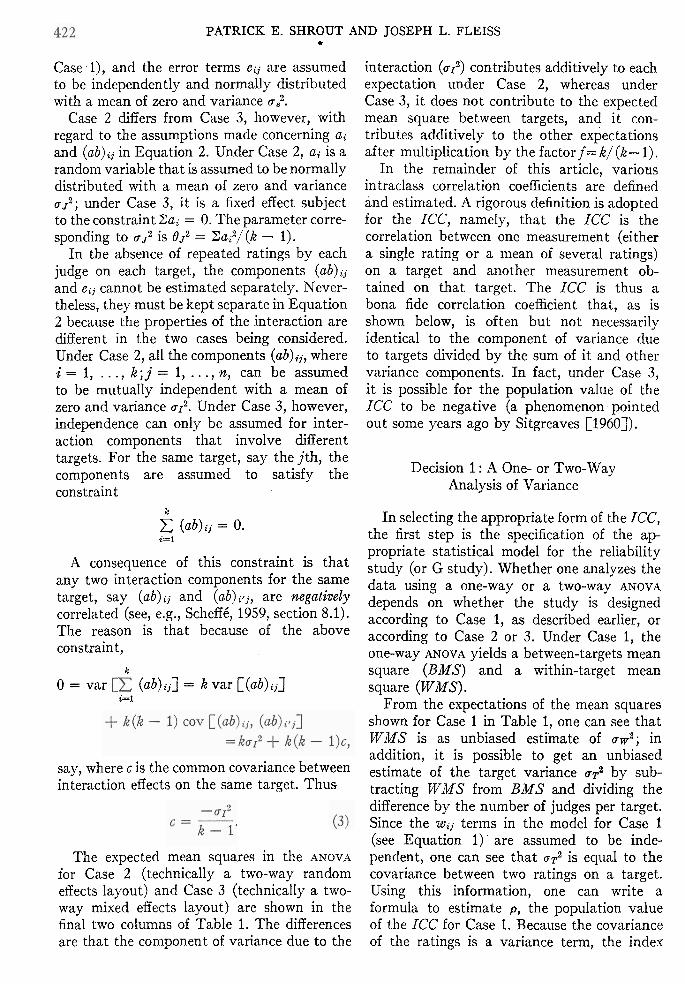
Table 4 Correlation Estimates From S i x ~ n t r a c l a s s Correlation Forms

Form Estimate

ICC (1, 1) .17 ICC (2, 1) .29 ICC (3, 1) .71 ICC (1,4) ' .44 ICC (2,4) .62 ICC (3 ,4) .91

from Case 2 or Case 3 studies is more likely. A consequence of this mistake is the under- estimation of the true correlation p. For the same set of data, ICC(1, 1) will, on the average, give smaller values than ICC (2, 1) or TCC (3,l).

To help the reader appreciate the differences among these coefficients and also among the two coefficients to be discussed later, we apply the various forms to an example. Table 2 gives four ratings on six targets, Table 3 shows the ANOVA table, and Table 4 gives the calculated correlation estimates for various cases.

Given the choice of the appropriate index, tests of the null hypothesis-that p = +can be made, and confidence intervals around the parameter can be computed. When using

ICC(1, I), the test that p is different from zero is provided by calculating Fo = BMSIWMS and testing it on (n - 1) and n(k - 1) degrees 'of freedom. A confidence interval for p can be computed as follows : Let F1-,(i, j ) denote the (1 - p) -100th percentile of the F distribution with i and j degrees of freedom, and define

FU = Fo.F1-+,[n(k - I), (n - I)] (4) and

FL = Fo/Fl-+,[(n - I), n(k - I)]. (5)

Then

FL - 1 Fu - 1 FL + (k - 1) < p < F u + (k- 1) (6)

is a (1 - a) - 100% confidence interval for p.

When ICC(2, 1) is appropriate, the signifi- cance test is again an F test, using F, = BMS/EMS on (n - 1) and (k - 1) (n - 1) degrees of freedom. The confidence interval for ICC (2, 1) is more complicated than that for ICC(1, I), since the index is a function of three independent mean squares. Following Satterthwaite (1946), Fleiss and Shrout (1978) have derived an approximate confidence interval. Let

where F J = JMS/EMS and = ICC(2, 1). If we define F* = FI-+,[(~ - I), v] and F, = F1-+u[~, (n - I)], then

n(BMS - F*EMS) n(F,BMS - EMS) F*[kJMS + (kn - k - n)EMS] + nBMS < < kJMS + (kn - k - n)EMS + nF,BMS ( 7 )

gives an approximate (1 - a ) 100% confi- dence interval around p.

Finally, when appropriate, ICC(3, 1) is tested with F, = BMSIEMS on (n - 1) and (n - 1) (k - 1) degrees of freedom. If we d e h e

then F L - 1 Fu - 1

FL + (k - 1) < < FU + (k - 1)

is a (1 - a). 100% confidence interval for p.

Decision 2: Can Effects Due to Judges Be Ignored in the Reliability Index?

In the previous section we stressed the importance of distinguishing Case 1 from Cases 2 and 3. In this section we discuss the choice between Cases 2 and 3. Most simply the choice is whether the raters are considered random effects (Case 2) or fixed effects (Case 3). Thus, under Case 2 we wish to generalize to other raters within. some population, whereas under Case 3 we are interested only in a single rater or a fixed set of k raters. Of course, once the appropriate case is identified,

INTRACLASS CORRELATIONS 425

the choice of indices is between ICC(2, 1) and ICC(3, I), as discussed before.

Most often, investigators would like to say that their rating scale can be effectively used by a variety of judges (Case 2), but there are some instances in which Case 3 is appropriate. Suppose that the reliability study (the G study) precedes a substantive study (the decision study in Cronbach et a1.k terms) in which each of the k judges is responsible for rating his or her own separate random sample of targets. If all the data in the final study are to be combined for analysis, the judges' effects will contribute to the variability of the ratings, and the random model with its associated ICC(2, 1) is appropriate. If, on the other hand, each judge's ratings are analyzed separately, and the separate results pooled, then interjudge variability will not have any effect on the final results, and the model of fixed judge effects with its associate ICC (3, 1) is appropriate.

Suppose that the substantive study involves a correlation between some reliable variable available for each target and the variable derived from the judges' ratings. One may either determine the correlation for the entire study sample or determine it separately for each judge's subsample and then pool the correlations using Fisher's z transformation. The variability of the judges' effects must be taken into account in the former case, but can be ignored in the latter.

Another example 'is a comparative study in which each judge rates a sample of targets from each of several groups. One may either compare the groups by combining the data from the k judges (in which case the component of variance due to judges contributes to variability, and the random effects model holds) or compare the groups separately for each judge and then pool the differences (in which case differences between the judges' mean levels 'of rating do not contribute to variability, and the model -of fixed judge effects holds).

When the judge variance is ignored, the correlation index can be interpreted in terms of rater consistency rather than rater agree- ment. Researchers of the rating process may choose between ICC(3, 1) and ICC(2, 1) on

the basis of which of these concepts they wish to measure. If, for example, two judges are used to rate the same n targets, the consistency of the two ratings is measured by ICC(3, I), treating the judges as fixed effects. To measure the agreement of these judges, ICC(2, 1) is used, and the judges are considered random effects; in this instance the question being asked is whether the judges are interchangeable.

Bartko (1976) advised that consistency is never an appropriate reliability concept for raters; he preferred to limit the meaning of rater reliability to agreement. Algina (1978) objected to Bartko's restriction, pointing out that generalizability theory encompasses the case of raters as fixed effects. Without directly addressing Algina's criticisms, Bartko (1978) reiterated his earlier position. The following example illustrates that Bartko's blanket restriction is not only unwarranted but can also be misleading.

Consider a correlation study in which one judge does all the ratings or one set of judges does all the ratings and their mean is taken. In these cases, judges are appropriately con- sidered fixed effects. If the investigator is interested in how much the correlations might be attenuated by lack of reliability in the ratings, the proper reliability index is ICC (3, I), since the correlations are not affected by judge mean differences in this case. In most cases the use of ICC(2, 1) will result in a lower value than when ICC(3, 1) is used. This relationship is illustrated in Tables 2, 3, and 4.

Although we have discussed the justification of using ICC(3, 1) with reference to the final analysis of a substantive study, in many cases the final analytic strategy may rest on the reliability study itself. Consider, for example, the case discussed above in which each judge rates a different subsample of targets. In this instance the investigator can either calculate 'correlations across the total sample or calculate them within subsamples and pool them. If the reliability study indicates a large dis- crepancy between ICC(2, 1) and ICC(3, I), the investigator may be forced to consider the latter analytic strategy, even though it involves a loss of degrees of freedom and a loss of computational simplicity.

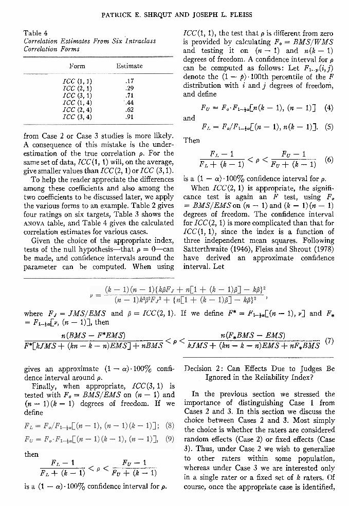
PATRICK E. SHROUT AND JOSEPH L. FLEISS .. Decision 3: What Is the Unit of Reliability? The index corresponding to ICC(1, 1) is

ICC(1, k) = (BMS - WMS)/BMS. Letting The ICC indices discussed so far give the F L and FU be defined as in Equations 4 and 5 ,

expected reliability of a single judge's ratings.' In the substantive study (D study), often it is 1 1 not the individual ratings that are used, but 1 - - < p < l - -

F L F u rather the mean of m ratings, where m need not be equal to k, the number of judges in the is a (1 - a) - 100% confidence interval for the reliability study (G study). In such a case population value of this intraclass correlation. the reliability of the mean rating is of interest; The index corresponding to IcC(~, 1) is this reliability will always be greater in magnitude than the reliability of the individual BMS - ELMS ratings, provided the latter is positive (cf. rCC(2, = BMS + (JMS - EMS),%- Lord & Novick, 1968).

Only occasionally is the choice of a mean rating as the unit of analysis based on sub- stantive grounds. An example of a substantive choice is the investigation of the decisions (ratings) of a team of physicians, as they are found in a hospital setting. More typically, an investigator decides to use a mean as a unit of analysis because the individual rating is too unreliable. In this case, the number of observations (say, m) used to form the mean should be determined by a reliability study in pilot research, for example, as follows. Given the lower bound, p ~ , on p from Inequality 6 or Inequality 7, whichever is appropriate, and given a value, say p*, for the minimum accept- able value for the reliability coefficient (e.g., p* = .75 or 30)) i t is possible to determine m as the smallest integer greater than or equal to

Once m is determined, either by a reliability study or by a choice made on substantive grounds, the reliability of the ratings averaged over m judges can be estimated using the Spearman-Brown formula and the appropriate ICC index described earlier. When data from m judges are actually collected (e.g., in the D study following the G study used to determine m), they can be used to estimate the reliabilities of the mean ratings in one step, using the formulas below. In these applications, k = m. The formulas correspond to . ICC(1, 1)) ICC(2, 1)) and ICC(3, I), and the significance test for each is the same as for their correspond- ing single-rater reliability index.

The confidence interval for this index is most easily obtained by using the confidence bounds obtained for ICC(2, 1) in the Spearman-Brown formula. For example, the lower bound for ICC(2, k) is

where PL** is the lower bound obtained for ICC(2, 1).

For ICC(3, I), the index of consistency for the mixed model case, the generalization from a single rating to a mean rating reliability is not quite as straightforward. Although the covariance between two ratings is - ur2/ (k - I) , the covariance between two means based on k judges is (rT2. AS we pointed out before, under Case 3 no estimator exists for this term.

If, however, the Judge X Target interaction can be assumed to be absent, then the ap- propriate index is

ICC(3, k) = (BMS - EMS)/BMS.

Letting F L and FU be defined as in Equations 8 and 9,

is .a (1 - a) - 100% confidence interval for the population value of this intraclass correlation. ICC(3, k) is equivalent to Cronbach's (1951) alpha; when the ratings of observers are dichotomous, it is equivalent to the Kuder- Richardson (1937) Formula 20.

INTRACLASS CORRELATIONS 42 7

Sometimes the choice of a unit of analysis causes a conflict between reliability considera- tions and substantive interpretations. A mean of k ratings might be needed for reliability, but the generalization of interest might be individuals.

For example, Bayes (1972) desired to relate ratings of interpersonal warmth to nonverbal communication variables. She reported the reliability of the warmth ratings based on the judgments of 30 observers on 15 targets. Because the rating variable that she related to the other variables was the mean rating over all 30 observers, she correctly reported the reliability of the mean ratings. With this index, she found that her mean ratings were reliable to .90. When she interpreted her findings, however, she generalized to single observers, not to other groups of 30 observers. This generalization may be problematic, since the reliability of the individual ratings was less than .30-a value the investigator did not report. In such a situation in which the unit of analysis is not the same as the unit general- ized to, i t is a good idea to report the relia- bilities of both units.

Conclusion

It is important to assess the reliability of judgments made by observers in order to know the extent that measurements are measuring anything. Unreliable measurements cannot be expected to relate to any other variables, and their use in analyses frequently violates Statistical assumptions. Intraclass correlation coefficients provide measures of reliability, but many forms exist and each is appropriate only in limited circumstances.

This article has discussed six forms of the intraclass correlation and guidelines for choos- ing among them. Important issues in the choice of an appropriate index include whether the ANOVA design should be one way or two way, whether raters are considered fixed or random effects, and whether the unit of analysis is a single rater or the mean of several raters. The discussion has been limited to a relatively pure data analysis case, k observers rating n targets with no missing data (i.e..

each of the n targets is rated by exactly k observers). Although we have implicitly limited the discussion to continuous rating scales, Feldt (1965) has reported that for ICC(3, k) a t least, the use of dichotomous dummy variables gives acceptable results. Readers interested in agreement indices for discrete data, however, should consult the Fleiss (1975) review of a dozen coefficients or the detailed review of coefficient kappa by Hubert (1977).

References

Algina, J. cornmeit on Bartko's "On various intraclass correlation reliability coefficients." Psychological Bulletin, 1978, 85, 135-138.

Bartko, J. J. The intraclass correlation coefficient as a measure of reliability. Psychological Reports, 1966, 19, 3-11.

Bartko, J. J. On various intraclass correlation reliability coefficients. Psychological Bulletin, 1976, 83, 762-765.

Bartko, J. J. Reply to Algina. Psychological Bulletin, 1978,85,139-140.

Bayes, M. A. Behavioral cues of interpersonal warmth. Journal of Consulting and Clinical Psyclzology, 1972, 39, 333-339.

Cronbach, L. J. Coefficient alpha and the internal structure of tests. Psyclzometrika, 1951, 16, 297-334.

Cronbach, L. J., Gleser, G. C., Nanda, H., & Rajarat- nam, N. The dependability of behavioral measurements. New York : Wiley, 1972.

Ebel, R. L. Estimation of the reliability of ratings. Psychometrika, 1951, 16, 407-424.

Feldt, L. S. The approximate sampling distribution of Kuder-Richardson reliability coefficient twenty. Psychometrika, 1965, 30, 357-370.

Fleiss, J. L. Measuring the agreement between two raters on the presence or absence of a trait. Bw- metrics, 1975, 31, 651-659.

Fleiss, J. L., & Shrout, P. E. Approximate interval estimation for a certain intraclass correlation coefficient. Psychonzetrika, 1978, 43, 259-262.

Haggard, E. A. Intraclass correlation and the analysis oj variance. New York: Dryden Press, 1958.

Hayes, W. L. Statistics for the social sciences. New York: Holt, Rinehart & Winston, 1973.

Hubert, L. Kappa revisited. Psychological Bulletin, . 1977, 84, 289-297. Kuder, G. F., & Richardson, M. W. The theory of the

estimation of test reliability. Psychometrika, 1937, 2, 151-160.

Lord, F. M., & Novick, M. R. Statistical theories of mental test scores. Reading, Mass. : Addison-Wesley 1968.

Olkin, I., & Pratt, J. W. Unbiased estimation of certain correlation coefficients. Annals of Mathe7natical Statistics, 1958, 29, 201-211.

PATRICK E. SHRQUT AND JOSEPH L. FLEISS

Rajaratnam, N. Reliability formulas for independent analysis of variance b y E. A. Haggard. Journal of the decision data when reliability data are matched. American Statistical Association, 1960, 55, 384-385. Psychonzetrika, 1960, 25, 261-271. Snedecor, G. W . , Sr Cochran, W . G. Statistical ~netltods

Satterthwaite, F. E. An approximate distribution o f (6th ed.). Ames, Iowa: State University Press, 1967. estimates of variance components. Biometries, 1946, Winer, B. J . Statistical principles i n experimental 2, 11C-114. Design (2nd ed.). New York : McGraw-Hill, 1971.

Scheff6, H. The analysis of variance. New York : Wiley, 1959.

Sitgreaves, R. Review of Intraclass correlation and the Received January 9 , 1978 m

lcek Ajzen E. James Anthony Barry C. Arnold Harold P. Bechtoldt Arthur L. Benton Carl Bereiter Allen E. Bergln R. Darrell Bock Robert C. Bolles Thomas D. Borkovec James H. Bryan Robert Cancro John A. Carpenter C. Richard Chapman Moncrieff Cochran Jacob Cohen Richard Darlington Robyn M. Dawes Arthur Dempster E. F. Diener Rlchard L. Doty Marvin D. Dunnette Phoebe C. Ellsworth Dorls R. Entwisle Albert Erlebacher Norman L. Farberow Donald W. Flske John H. Fiavell Joseph L. Flelss Bennett G. Gaief, Jr. Paul A. Games Goldlne C. Gleser

Editorial Consultants for This Issue

Lewls R. Goldberg Quinn McNemar Harrison G. Gough Ivan W. Mlller Ill James E. Grizzle James S. Myer J. Richard Hackman Jerome L. Myers Marshall M. Haith Theodore Munsat Richard J. Harrls John R. Nesselroade James B. Heltler Bernice L. Neugarten Jullan Hochberg Jum C. Nunnally Jerry A. Hogan Ellis Page Eric W. Holman Morrls B. Parloff Philip Holzman Robert M. Pruzek Lawrence J. Hubert J. 0. Ramsay Janet Hyde Samuel H. Revusky Douglas R. Jackson Robert Rosenthal H. Royden Jones, Jr. William W. Rozeboom James W. Kalat Robert T. Rubln Anthony Kales Herman C. Salzberg Daniel P. Keating Davld J. Schnelder H. J. Keselman Gerard Schnelder Helena Chmura Kraemer Lee Sechrest Michael J. Larnbert Dean Keith Simonton Edward E. Lawler 111 Barbara Sommer Paul R. Lawrence Richard M. Sorrentlno Kenneth J. Levy Donald P. Spence James C. Lingoes Hans Strupp Robert L. Linn Robert L. Thorndike John C. Loehlln George E. Vaillant Frederick J. Manning Rebecca Warner Leonard A. Marascullo Bernard Welner Ellen Markman Leland Wllkinson Steven W. Matthysse Arthur J. Woodward David McNelll Paul M. Wortman