1

Interval Estimation for Conditional Failure Rates ofTransmission Lines with Limited Samples

Ming Yang, Member, IEEE, Jianhui Wang, Senior Member, IEEE, Haoran Diao, Student Member, IEEE,Junjian Qi, Member, IEEE, and Xueshan Han

Abstract—The estimation of the conditional failure rate (CFR)of an overhead transmission line (OTL) is essential for powersystem operational reliability assessment. It is hard to predictthe CFR precisely, although great efforts have been made toimprove the estimation accuracy. One significant difficulty is thelack of available outage samples, due to which the law of largenumbers is no longer applicable and no convincing statisticalresult can be obtained. To address this problem, in this paper anovel imprecise probabilistic approach is proposed to estimate theCFR of an OTL. The imprecise Dirichlet model (IDM) is appliedto establish the imprecise probabilistic relation between a singleconditional variable and the failure rate of an OTL. Then a credalnetwork is constructed to integrate the IDM estimation resultscorresponding to different conditional variables and infer theCFR. Instead of providing a single-valued estimation result, theproposed approach predicts the possible interval of the CFR inorder to explicitly indicate the uncertainty of the estimation andmore objectively represent the available knowledge. The proposedapproach is illustrated by estimating the CFRs of two LGJ-300transmission lines located in the same region; the test resultsvalidate its effectiveness.

Index Terms—Credal network, failure rate estimation, impre-cise Dirichlet model, imprecise probability, overhead transmissionline, reliability.

I. INTRODUCTION

ESTIMATION of the failure rates of overhead transmissionlines (OTLs) is crucial for power system reliability as-

sessment, maintenance scheduling, and operational risk control[1], [2]. The failure rates of OTLs are usually assumed to beconstant and are estimated using the long-term mean values.However, in reality they can be significantly influenced byboth external and internal operational conditions [3]. Thepredominant influential factors include the aging of the OTL,the loading level, and external environmental conditions.

Over the last few decades, substantial work has been doneon the conditional failure rate (CFR) estimation with respect tovarious operational conditions. In [4], the weather conditionsare divided into three classes, i.e., normal, adverse and major

This work was supported in part by the National Science Foundation ofChina under Grant 51007047 and Grant 51477091 and in part by the NationalBasic Research Program of China (973 Program) under Grant 2013CB228205.

M. Yang is with Key Laboratory of Power System Intelligent Dispatchand Control, Shandong University, Jinan, Shandong 250061 China. He is alsoworking as a research assistant with Argonne National Laboratory, Argonne,IL 60439 USA (e-mail: myang@sdu.edu.cn).

J. Wang and J. Qi are with the Energy Systems Division, ArgonneNational Laboratory, Argonne, IL 60439 USA (e-mail: jianhui.wang@anl.gov;jqi@anl.gov).

H. Diao and X. Han are both with Key Laboratory of Power SystemIntelligent Dispatch and Control, Shandong University, Jinan, Shandong250061 China (e-mail: shanda10dhr@gmail.com; xshan@sdu.edu.cn).

adverse, in order to count the failures occurring under differentweather conditions. The influences of multiple weather regionson the failure rate and repair rate of a single transmissionline are modeled in [5]. In [6], the Poisson regression modeland Bayesian network model are applied to estimate theunconditional and conditional failure rates of overhead dis-tribution lines. Weather-related fuzzy models of failure rate,repair time and unavailability of OTLs are established in[7]. The failure rate under both normal and adverse weatherconditions is expressed by a fuzzy number in this paper.It is pointed out in [8] that systems with aged componentsmight experience higher than average incidence of failures.By using the data collected from Electricity of France, theeffects of aging and weather conditions on transmission linefailure rates are analyzed in [9], where the influences of thewind speed, temperature, humidity, and lightning intensity areexamined. In [10], the time-varying failure rates are discussedby considering the effects of adverse weather and componentaging, and data collection efforts for non-constant failure rateestimation are suggested. In [11], the failure rates are modeledfor different loading levels and the occurrence of variousloading levels is represented by a two-stage renewal process.

Although great efforts have been made to improve the CFRestimation accuracy, it is still difficult if not impossible toget convincing CFR estimation results. The major barrier isthe lack of historical outage observations under the relevantoperational conditions. In this situation, the law of largenumbers is no longer applicable and a precise estimation ofthe failure rate cannot be obtained. This data-deficient problemmight be trivial for the constant failure rate estimation, butis crucial for the condition-related failure rate prediction.In fact, the uncertainty of the failure rate estimation withlimited samples has already been recognized, and the mostrepresentative approach to solving this problem is the fuzzymodel proposed by Li et al. [7]. However, this instructiveapproach still relies on a precise Chi-square distribution, whichcan hardly be obtained in practice, to set up the fuzzy outagemodel. It has to be admitted that the data-deficient problem ofthe CFR estimation has not been well addressed till now.

In this paper, a novel imprecise probabilistic approach isproposed to estimate the CFR of an OTL. The failure in aspecified time interval is represented by a random variablefollowing the binomial distribution. Instead of providing asingle-valued CFR estimation result, the proposed approachpredicts the possible interval of the CFR with limited historicalobservations, and thus can reflect the available estimationinformation more objectively. An imprecise statistical algo-

arX

iv:1

601.

0634

4v1

[st

at.A

P] 2

4 Ja

n 20

16

2

rithm called imprecise Dirichlet model (IDM) is adoptedto estimate the imprecise probabilistic relation between thefailure rate of an OTL and one kind of operational condition.Then a credal network that can perform imprecise probabilisticreasoning is established to integrate the IDM estimation resultscorresponding to different operational conditions and to obtainthe interval of the CFR. The advantages of the proposedapproach include the following:

1) IDM is an efficient statistical approach for drawing outimprecise probabilities from available data. By usingIDM, the uncertainty of the probabilistic dependencyrelation between an operational condition and the failurerate can be quantitatively reflected by the width of theprobability interval.

2) The credal network is a flexible probabilistic inferenceapproach based on imprecise probabilities. Various oper-ational conditions that have either precise or impreciseprobabilistic relations with the failure rate can be si-multaneously considered in the network. Moreover, theoccurrence probabilities of these conditions can also berepresented conveniently.

3) The proposed approach can truthfully reflect the infor-mation contained in the data. By combining IDM andthe credal network, the approach explicitly models theuncertainty of the estimated CFR. When sufficient fail-ure observations are available, the uncertainty intervalof the CFR may shrink to a single point, in which casea single-valued CFR estimation result will be obtained.

The rest of this paper is organized as follows: In SectionII a binomial failure rate estimation model is introduced.Section III discusses mathematical foundations of the proposedapproach. Details of CFR estimation are provided in SectionIV. Case studies are presented in Section V and conclusionsare drawn in Section VI.

II. MODEL OF FAILURE RATE ESTIMATION

A. Failure Rate Basics

Failure rate is a widely applied reliability parameter thatrepresents the frequency of component failures [12]. Mathe-matically, the failure rate at time t can be expressed as

λ(t) = lim∆t→0

Prt < Tf ≤ t+ ∆t|Tf > t

∆t

= lim∆t→0

F (t+ ∆t)− F (t)(1− F (t)

)·∆t

(1)

where λ(t) is the failure rate at time t, PrA|B is theconditional probability of event A given event B, Tf is thefailure time, F (t) = Pr0 ≤ Tf ≤ t is the cumulative failuredistribution, and ∆t is a small time interval.

As expressed in Eq. (1), the failure rate indicates an in-stantaneous probability that a normally operating componentbreaks down at time t. In practice, the failure rate is usuallyapproximated by the average failure probability within a smalltime interval (t, t+∆t]. This approximation will have sufficientaccuracy when ∆t is so small that the failure rate can beconsidered as constant within the time interval. In this paper,hourly OTL failure rates are investigated and thus ∆t is

correspondingly set to 1 hour. Since the time scale is verysmall compared with the whole life of OTLs, the hourly failurerate of an OTL can be approximately represented by

λ(t) ≈ Prt < Tf ≤ t+ 1|Tf > t

(2)

where λ(t) is the failure rate in the tth hour and Prt < Tf ≤t+ 1|Tf > t is the probability that the OTL fails in the timeinterval (t, t+ 1].

B. Binomial Model for the Failure Rate Estimation

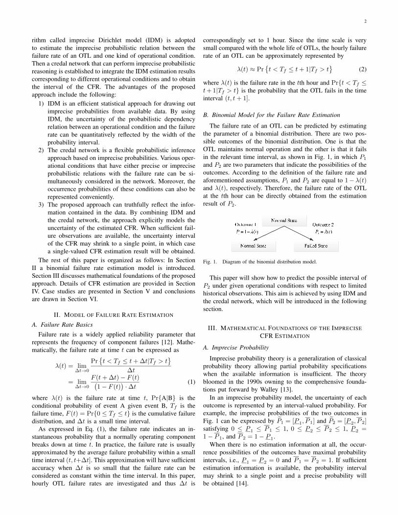
The failure rate of an OTL can be predicted by estimatingthe parameter of a binomial distribution. There are two pos-sible outcomes of the binomial distribution. One is that theOTL maintains normal operation and the other is that it failsin the relevant time interval, as shown in Fig. 1, in which P1

and P2 are two parameters that indicate the possibilities of theoutcomes. According to the definition of the failure rate andaforementioned assumptions, P1 and P2 are equal to 1−λ(t)and λ(t), respectively. Therefore, the failure rate of the OTLat the tth hour can be directly obtained from the estimationresult of P2.

Fig. 1. Diagram of the binomial distribution model.

This paper will show how to predict the possible interval ofP2 under given operational conditions with respect to limitedhistorical observations. This aim is achieved by using IDM andthe credal network, which will be introduced in the followingsection.

III. MATHEMATICAL FOUNDATIONS OF THE IMPRECISECFR ESTIMATION

A. Imprecise Probability

Imprecise probability theory is a generalization of classicalprobability theory allowing partial probability specificationswhen the available information is insufficient. The theorybloomed in the 1990s owning to the comprehensive founda-tions put forward by Walley [13].

In an imprecise probability model, the uncertainty of eachoutcome is represented by an interval-valued probability. Forexample, the imprecise probabilities of the two outcomes inFig. 1 can be expressed by P1 = [P 1, P 1] and P2 = [P 2, P 2]satisfying 0 ≤ P 1 ≤ P 1 ≤ 1, 0 ≤ P 2 ≤ P 2 ≤ 1, P 2 =1− P 1, and P 2 = 1− P 1.

When there is no estimation information at all, the occur-rence possibilities of the outcomes have maximal probabilityintervals, i.e., P 1 = P 2 = 0 and P 1 = P 2 = 1. If sufficientestimation information is available, the probability intervalmay shrink to a single point and a precise probability willbe obtained [14].

3

B. Imprecise Dirichlet Model

IDM is an efficient method for imprecise probability cal-culation with multinomial data [15]. It is an extension of thedeterministic Dirichlet model.

Consider a multinomial distribution which has M typesof outcomes. To estimate the occurrence probabilities of theoutcomes, the deterministic Dirichlet model uses a Dirichletdistribution as the prior distribution, which is

f(P1, · · · , PM ) =Γ(∑M

m=1 am

)∏M

m=1 Γ(am)

M∏m=1

P am−1m (3)

where P1, P2, · · · , PM are the probabilities of the outcomes,a1, a2, · · · , aM are the positive parameters of the Dirichletdistribution and Γ is the gamma function.

Since the Dirichlet distribution is a conjugate prior ofthe multinomial distribution, the posterior of P1, P2, · · · , PM

with respect to the observations also belongs to a Dirichletdistribution, which can be represented as

f(P1, · · · , PM )

=Γ(∑M

m=1 am

)+∑M

m=1 nm∏Mm=1 Γ(am + nm)

M∏m=1

P am+nm−1m (4)

where nm, m = 1, 2, . . . ,M , is the number of times that themth outcome is observed.

Therefore, the parameters of the multinomial distributioncan be estimated by the expected values of the posteriordistribution, as

Pm =nm + am∑M

m=1 nm +∑M

m=1 amm = 1, 2, . . . ,M. (5)

By analyzing the estimation results of the determinis-tic Dirichlet model, it can be found that Pm will beam/

∑Mm=1 am if no available observations exist. This value

is the prior estimation of the occurrence possibility of the mthoutcome. Here the parameter am is called the prior weight ofthe outcome, and

∑Mm=1 am is usually denoted by s, which is

called the equivalent sample size. In the parameter estimationprocess, s implies the influence of the prior on the posterior.The larger s is, the more observations are needed to tune theparameters assigned by the prior distribution.

Equation (5) provides a feasible approach for the multino-mial parameter estimation. However, in practice the availableobservations may be scarce (like the OTL outage obser-vations). In this case, the prior weights will significantlyinfluence the parameter estimation results, which will be toosubjective to be useful.

To avoid the shortcomings of the deterministic Dirichletmodel, IDM uses a set of prior density functions instead of asingle density function [16], which can be described as

f(P1, · · · , PM ) =Γ(s)∏M

m=1 Γ(s · rm)

M∏m=1

P s·rm−1m

∀rm ∈ [0, 1],

M∑m=1

rm = 1 (6)

where rm, m = 1, 2, . . . ,M , is the mth prior weight factor.

In (6), s · rm plays the same role as am in Eq. (3). Whenrm varies in the interval [0, 1], the set will contain all of thepossible priors given a predetermined s and the prejudice ofthe prior can thus be avoided.

Then the corresponding posterior density function set canbe calculated according to Bayesian rules, as

f(P1, · · · , PM ) =Γ(s+ n)∏M

m=1 Γ(s · rm + nm)

M∏m=1

P s·rm+nm−1m

∀rm ∈ [0, 1],

M∑m=1

rm = 1 (7)

where n =∑M

m=1 nm is the number of total observations.Therefore, the imprecise parameters of the multinomial dis-

tribution can be estimated from the posterior density functionset as

Pm = [Pm, Pm] =

[nmn+ s

,nm + s

n+ s

]m = 1, 2, . . . ,M.

(8)

The bounds of the probability intervals in Eq. (8) arecalculated with respect to the bounds of rm, m = 1, 2, . . . ,M ;and more theoretical details can be found in [13].

In (8), s is the only exogenous parameter to be specified,and it is set to 1 in our model as suggested by [14].

C. Credal Network

The credal network is developed from the Bayesian network,which is a popular graphical model representing the probabilis-tic relations among the variables of interest [17], [18].

In a Bayesian network, each node stands for a categoricalvariable while arcs indicate the dependency relations amongthe variables. During the modeling process of a Bayesiannetwork, a conditional mass function P (Xi|πi) should bespecified for each Xi ∈ X and πi ∈ ΩΠi

, where X standsfor all of the categorical variables of the network, Xi is the ithcategorical variable, Πi stands for the parent variables of Xi,ΩΠi

is the value space of Πi, and πi is the joint observationvalue of Πi.

A simple credal network with four nodes and three arcsis shown in Fig. 2, in which the uppercase characters standfor the two-state categorical variables while the lowercasecharacters stand for the observation values of the variables.All of the necessary conditional mass functions for inferencehave been provided in the figure.

Fig. 2. Diagram of a simple Bayesian network.

4

Because all of the marginal and conditional mass functionshave been included, a Bayesian network can be essentiallyregarded as a joint mass function over X which can befactorized as P (x) =

∏Ii=1 P (xi|πi) for each x ∈ ΩX , where

I is the number of nodes in the network, xi is an observationof Xi, x is a joint observation value of X and ΩX is thevalues space of X .

Therefore, with given evidences XE = xE , the conditionalprobability of an outcome of the queried variable Xq can beestimated according to Bayesian rules as

P (xq|xE) =P (xq,xE)

P (xE)=

∑XM

∏Ii=1 P (xi|πn)∑

XM ,Xq

∏Ii=1 P (xi|πn)

(9)

where XM ≡X \ (XE ∪Xq) and∑

XMmeans calculating

the total probability with XM [18].For instance, consider the network shown in Fig. 2. With

the evidences G = g, H = h and R = r, the probability ofQ = q can be calculated as

P (q|g, h, r) =P (q, g, h, r)

P (g, h, r)

=P (g)P (h)P (r|h)P (q|g, h)

P (g)P (h)P (r|h)P (q|g, h) + P (g)P (h)P (r|h)P (qc|g, h)

=P (g)P (h)P (r|h)P (q|g, h)

P (g)P (h)P (r|h)= 0.5.

The credal network relaxes the Bayesian network by ac-cepting imprecise probabilistic representations [19], [20]. Thedifferences between the credal network and the Bayesiannetwork lie in the following three levels:

1) The probability corresponding to each outcome: In aBayesian network, each outcome of a categorical variable has asingle-valued probability. On the contrary, in a credal network,the occurrence chance for each outcome can be represented byan interval-valued probability.

2) The mass function of each categorical variable: Acategorical variable described by imprecise probabilities hasa set of mass functions instead of just one. The convex hullof the mass function set is defined as a credal set [20], [21],which can be expressed as

K(Xi) = CHP (Xi) : for each xi ∈ ΩXi

,

P (xi) ∈[P (xi), P (xi)

]and

∑ΩXi

P (xi) = 1

(10)

where K(Xi) is the credal set of Xi, CH means the followingset is a convex hull, P (Xi): Descriptions is a set ofprobability mass functions specified by the descriptions, ΩXi

is the value space of Xi, and∑

ΩXiP (xi) = 1 means the sum

of the probabilities for all outcomes should be equal to 1.Although the credal set contains an infinite number of

mass functions, it only has a finite number of extrememass functions, which are denoted by EXT[K(Xi)]. Theseextreme mass functions correspond to the vertexes of theconvex hull and can be obtained by combining the endpointsof the probability intervals. For instance, assume P (g) andP (gc) in Fig. 2 are imprecise, i.e., P (g) ∈ [0.2, 0.4] andP (gc) ∈ [0.6, 0.8]. In this case, the mass function P (G) can beany combination of P (g) and P (gc) satisfying the constraint

P (g) + P (gc) = 1. However, P (G) only has two extrememass functions, which are P (g) = 0.2, P (gc) = 0.8 andP (g) = 0.4, P (gc) = 0.6.

The inference over a credal network is based on theconditional credal set K(Xi|πi), i = 1, 2, . . . , I . And it isequivalent to an inference based only on the extreme massfunctions of the conditional credal sets.

3) The joint mass function of the network: While aBayesian network defines a joint mass function, a credalnetwork defines a joint credal set that contains a collection ofjoint mass functions [22]. The convex hull of these joint massfunctions is called a strong extension of the credal network,and can be formulated as

K(X) = CHP (X) : for each x ∈ ΩX ,

P (x) =∏I

i=1P (xi|πi), P (Xi|πi) ∈ K(Xi|πi)

(11)

where K(X) is the strong extension of the credal network,P (X): Descriptions is a set of joint mass functions specifiedby the descriptions, and P (Xi|πi) ∈ K(Xi|πi) indicates thatthe conditional mass function P (Xi|πi) should be selectedfrom the conditional credal set K(Xi|πi).

Observe from Eq. (11) that the joint probability P (x) is im-precise since each P (xi|πi), whose mass function P (Xi|πi)can be arbitrarily selected from the credal set K(Xi|πi),is imprecise. For this reason, K(X) contains a set of jointmass functions. On the other hand, when the mass functionP (Xi|πi), i = 1, 2, . . . , I , is selected, the joint probability ofP (x) for each x ∈ ΩX will be determined, and hence onedeterministic joint mass function P (X) will be obtained. Itis easy to imagine that each joint mass function of a strongextension corresponds to a Bayesian network.

If P (Xi|πi) can only be selected from the extreme massfunctions of K(Xi|πi), then the resulting joint mass functionsare called the extreme joint mass functions, and they corre-spond to the vertexes of the strong extension. The extremejoint mass functions EXT[K(X)] can be obtained by

EXT[K(X)] =P (X) : for each x ∈ ΩX ,

P (x) =∏I

i=1P (xi|πi)

P (Xi|πi) ∈ EXT[K(Xi|πi)]. (12)

On the basis of the aforementioned features, it can beseen that the credal network has a significant association withthe Bayesian network. The intent of inference over a credalnetwork is to compute the bounds of the imprecise probabilityfor each outcome of Xq respecting XE = xE . And thisaim can be achieved by inferring over the Bayesian networkscorresponding to the extreme joint mass functions of the strongextension, as

P (Xq = xq|XE = xE)

= maxP (X)∈EXT[K(X)]

P (Xq = xq,XE = xE)

P (XE = xE)

P (Xq = xq|XE = xE)

= minP (X)∈EXT[K(X)]

P (Xq = xq,XE = xE)

P (XE = xE)(13)

5

where P (X) ∈ EXT[K(X)] indicates that P (X) should beselected from the extreme joint mass functions of K(X).

It can be clearly seen from Eq. (13) that when an extremejoint mass function is selected, Eq. (13) will become aBayesian network inference problem which can be conve-niently solved by Eq. (9). Therefore, the inference over acredal network can be executed by performing the followingfour steps:

1) For each categorical variable Xi with given πi,calculate its extreme conditional mass functionsEXT[K(Xi|πi)] by combining the probability intervalendpoints P (xi|πi) and P (xi|πi) of each xi ∈ ΩXi .

2) Form the extreme joint mass functions EXT[K(X)]with respect to the extreme conditional mass functionsEXT[K(Xi|πi)], i = 1, 2, . . . , I , πi ∈ ΩΠi

, accordingto Eq. (12).

3) Infer on each extreme joint mass function inEXT[K(X)] with given evidences XE = xE and ob-tain the conditional probability P (Xq = xq|XE = xE)according to Eq. (9).

4) Find the maximum and minimum probabilities ofP (Xq = xq|XE = xE) with respect to the inferenceresults of all the extreme joint mass functions.

IV. DETAILS OF THE IMPRECISE CFR ESTIMATION

A. Imprecise CFR Estimation Model

The failure rate of an OTL has a close relationship withsurrounding weather conditions. An OTL is more likely tobreak down in adverse weather conditions, e.g., high ambientair temperature, strong wind, heavy rains, or lightning storms.The loading condition can also influence the failure rate ofan OTL. When carrying heavy load, an OTL may suffer froma higher probability of a short-circuit fault [11]. Moreover,the failure rate may change gradually with the age of anOTL. Aged transmission lines usually have a relatively higherfailure rate under the same weather and loading conditions.Taking these observations into account, a credal network isestablished for estimating the CFR of an OTL, as shown inFig. 3. In the figure, the operational conditions are denoted bythe categorical variables E1, E2, · · · , E5, and the operationalsituation of the OTL is indicated by the binary variable H .

Fig. 3. Credal network for imprecise CFR estimation.

The dependency relations between the OTL situation and theoperational conditions are reflected by the conditional credalsets K(Ei|H) for i = 1, 2, 3, 5 and K(E4|H,E3). It shouldbe emphasized that the relation between the rain and lightning

is also reflected in the network, since lightning is more likelyto occur on a rainy day.

The aging of the OTL is not explicitly included in thenetwork but is reflected by the long-term average failure rate,which will serve as a prior probability in the proposed model.The states of the categorical variables are listed in Table I, inwhich T is the hourly average temperature, W is the hourlyaverage wind speed, and L is the hourly average loading rate.

TABLE ISTATES OF THE CATEGORICAL VARIABLES

Variables State 1 State 2 State 3

E1T ≤4°C

(e1,1)4°C< T ≤26°C

(e1,2)T >26°C

(e1,3)

E2W ≤12km/h

(e2,1)12km/h< W ≤40km/h

(e2,2)T >40km/h

(e2,3)

E3Rain

(e3,1)No Rain

(e3,2)N/A

E4Lightning

(e4,1)No Lightning

(e4,2)N/A

E5L ≤ 80%

(e5,1)L > 80%

(e5,2)N/A

HNormal Operation

(h1)Breaking Down

(h2)N/A

B. Estimation of the Extreme Mass Functions

Estimating the extreme mass functions of the credal setsK(Ei|H) for i = 1, 2, 3, 5 and K(E4|H,E3) is the first stepfor the CFR inference. To achieve this purpose, the endpointsof the conditional probabilities corresponding to the outcomesof P (Ei|H) for i = 1, 2, 3, 5 and P (E4|H,E3) have to firstbe calculated using IDM, as expressed in Eq. (8).

For instance, to estimate the extreme mass functions ofthe conditional credal set K(E5|h2), which describes theuncertainty of the loading condition when the transmission linefails, the endpoints of the probability intervals correspondingto P (e5,1|h2) and P (e5,2|h2) have to be calculated via Eq.(8), as

P (e5,1|h2) =ne,(5,1)(h,2)

nh,2 + s, P (e5,1|h, 2) =

ne,(5,1)(h,2) + s

nh,2 + s

P (e5,2|h2) =ne,(5,2)(h,2)

nh,2 + s, P (e5,2|h, 2) =

ne,(5,2)(h,2) + s

nh,2 + s

where ne,(5,1)(h,2) and ne,(5,2)(h,2) are the numbers of samplesfor which the OTL breaks down in the relevant time intervalwith a normal and high loading level, respectively, and nh,2 =ne,(5,1)(h,2) +ne,(5,2)(h,2) is the number of samples for whichthe OTL breaks down in the relevant time interval.

Then the conditional credal set K(E5|h2) can be obtainedfrom Eq. (10) as

K(E5|h2) = CHP (E5|h2) :

P (e5,1|h2) ∈ [P (e5,1|h2), P (e5,1|h2)],

P (e5,2|h2) ∈ [P (e5,2|h2), P (e5,2|h2)],

P (e5,1|h2) + P (e5,2|h2) = 1.

Also, the extreme mass functions of the credal set canbe obtained by combining the endpoints of the probability

6

intervals as

EXT[K(E5|h2)] =P (e5,1|h2) = P (e5,1|h2), P (e5,2|h2) = P (e5,2|h2)

and

P (e5,1|h2) = P (e5,1|h2), P (e5,2|h2) = P (e5,2|h2)

.

Other conditional credal sets and corresponding extrememass functions can be calculated in the same way.

C. Imprecise CFR Inference with the Credal Network

With respect to the credal network mentioned above, thebounds of CFR under specified operational conditions can becalculated according to Eqs. (9), (12) and (13), as

λ = P (h2|e)

= max

∏j=1,2,3,5

P (ej,kj |h2) · P (e4,k4 |h2, e3,k3) · P (h2)∑i=1,2

∏j=1,2,3,5

P (ej,kj|hi) · P (e4,k4

|hi, e3,k3) · P (hi)

λ = P (h2|e)

= min

∏j=1,2,3,5

P (ej,kj|h2) · P (e4,k4

|h2, e3,k3) · P (h2)∑

i=1,2

∏j=1,2,3,5

P (ej,kj|hi) · P (e4,k4

|hi, e3,k3) · P (hi)

P (Ej |hi) ∈ EXT[K(Ej |hi)],P (E4|hi, e3,k3) ∈ EXT[K(E4|hi, e3,k3)];

i = 1, 2; j = 1, 2, 3, 4, 5;

when j = 1, 2, kj = 1, 2, 3;

when j = 3, 4, 5, kj = 1, 2 (14)

where i is the index of the states of OTL, j is the index ofthe evidence variables, kj is the index of the states of the jthevidence variable. P (h2) is the prior probability of h2, whichcan be estimated using the average failure rate of OTLs atspecified age, P (h1) = 1−P (h2), P (ej,kj

|hi) means the con-ditional probability of the observation ej,kj

given hi with re-spect to the conditional mass function P (Ej |hi), P (Ej |hi) ∈EXT[K(Ej |hi)] indicates that the conditional mass functionP (Ej |hi) should be selected from the extreme mass func-tions of the credal set K(Ej|hi), P (e4,k4|hi, e3,k3) meansthe conditional probability of the observation e4,k4 givenhi and e3,k3 with respect to the conditional mass functionP (E4|hi, e3,k3), and P (E4|hi, e3,k3) ∈ EXT[K(E4|hi, e3,k3)]indicates that the conditional mass function P (E4|hi, e3,k3)should be selected from the extreme mass functions of thecredal set K(E4|hi, e3,k3).

In (14), P (ej,kj |h2) is the occurrence probability of thecondition ej,kj , e.g., high temperature e1,3, given OTL failureis observed. Considering the deficiency of the failure samples,the probability should be represented in an imprecise form,which can be obtained by using IDM. On the other hand,P (ej,kj

|h1) is the occurrence probability of the conditiongiven no OTL failure happens. In this case, abundant samplesare available since no failure is a large probability event.Therefore, this probability can be represented in a preciseform, which can be approximated using the average occurrenceprobability of the condition, e.g., P (e1,3|h1) ≈ P (e1,3) can

be approximated using the average high temperature rate inthe region. The conditional probabilities P (e4,k4|h1, e3,k3) andP (e4,k4|h2, e3,k3) can be obtained in the same way. Obviously,since the precise probability is a special case of the impreciseprobability, the CFR can still be estimated using Eq. (14) underthis circumstance.

V. CASE STUDIES

The proposed approach is tested by estimating the CFRs oftwo LGJ-300 transmission lines located in the same region.One of the transmission lines, which is denoted as TL1,has been in operation for 5 years. The recent three-yearaverage failure rate is 0.00027 times per hour. As a result,the parameters P (h1) and P (h2) of TL1 are 0.99973 and0.00027, respectively. The other transmission line, denoted asTL2, has been in operation for 10 years, and its three-yearaverage failure rate is 0.00042 times per hour. Therefore, theparameters P (h1) and P (h2) of TL2 are 0.99958 and 0.00042,respectively.

A. CFR Estimation by the Deterministic Inference Approach

With historical records, deterministic CFR estimation can beperformed by using the classical Bayesian network expressedby Eq. (9). On the basis of the samples collected from TL1

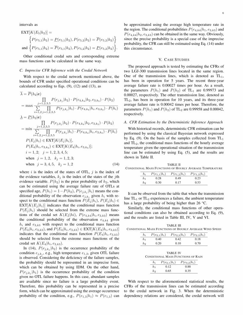
and TL2, the conditional mass functions of the hourly averagetemperature given the operational situation of the transmissionline can be estimated by using Eq. (5), and the results areshown in Table II.

TABLE IICONDITIONAL MASS FUNCTIONS OF HOURLY AVERAGE TEMPERATURE

hi P (e1,1|hi) P (e1,2|hi) P (e1,3|hi)

h1 0.28 0.49 0.23h2 0.30 0.17 0.53

It can be observed from the table that when the transmissionline TL1 or TL2 experiences a failure, the ambient temperaturehas a large probability of being higher than 26 °C.

Similarly, the conditional mass functions of other opera-tional conditions can also be obtained according to Eq. (9),and the results are listed in Table III, IV, V and VI.

TABLE IIICONDITIONAL MASS FUNCTIONS OF HOURLY AVERAGE WIND SPEED

hi P (e2,1|hi) P (e2,2|hi) P (e2,3|hi)

h1 0.40 0.42 0.18h2 0.20 0.10 0.70

TABLE IVCONDITIONAL MASS FUNCTIONS OF RAIN

hi P (e3,1|hi) P (e3,2|hi)

h1 0.12 0.88h2 0.65 0.35

With respect to the aforementioned statistical results, theCFRs of the transmission lines can be estimated accordingto the credal network in Fig. 3. When the deterministicdependency relations are considered, the credal network will

7

TABLE VCONDITIONAL MASS FUNCTIONS OF LIGHTNING

hi e3,k3P (e4,1|hi, e3,k3

) P (e4,2|hi, e3,k3)

h1 e3,1 0.33 0.67h2 e3,1 0.63 0.37h1 e3,2 0.02 0.98h2 e3,2 0.11 0.89

TABLE VICONDITIONAL MASS FUNCTIONS OF HOURLY AVERAGE LOADING RATE

hi P (e5,1|hi) P (e5,2|hi)

h1 0.67 0.33h2 0.55 0.45

be simplified to a Bayesian network. To illustrate this esti-mation approach, three scenarios under different operationalconditions are tested.

Scenario I: The transmission line TL1 is operating normallynow. Its average loading rate will be 95% in the next hour. Atthe same time, according to the short-term weather forecast,a thunderstorm will come in the next hour. During the storm,the average air temperature will be 30°C and the wind speedwill reach up to 48 km/h. Find the CFR of TL1 for the cominghour.

Scenario II: The transmission line TL1 is operating nor-mally now. In the next hour the temperature will be 15°C,the wind speed will be 10 km/h and the loading rate of thetransmission line will be less than 45%. Find the CFR of TL1

for the coming hour.Scenario III: The transmission line TL2 is operating nor-

mally now. All the operational conditions are the same asScenario I. Estimate the CFR of TL2 under this scenario.

The CFRs estimated according to the Bayesian network areshown in Table VII.

TABLE VIIESTIMATION RESULTS OF THE BAYESIAN NETWORK

Scenario I Scenario II Scenario III3.3E−2 1.4E−5 5.0E−2

It can be observed from the estimation results that theCFR of TL1 under Scenario I is much higher than that underScenario II. This is because all the operational conditions ofScenario I are adverse to the power transmission comparedwith that of Scenario II. On the other hand, it can be foundfrom the results of Scenario I and Scenario III that the CFR ofTL2 is much higher than that of TL1 under the same weatherand loading conditions. TL2 has a higher CFR because it hasbeen in service longer.

B. CFR Estimation by the Proposed Approach

Because the failure samples are scarce in practice, the con-ditional mass functions of the operational conditions countedwith respect to the failure samples may be unreliable. There-fore, IDM is applied here to estimate these imprecise condi-tional mass functions to quantitatively reflect the uncertaintyof the estimation results.

Using the historical observations, the imprecise conditionalmass functions given OTL failures can be obtained using Eq.(8), and the results are listed in Table VIII, IX, X, XI and XII.

TABLE VIIIIMPRECISE CONDITIONAL MASS FUNCTIONS OF HOURLY AVERAGE

TEMPERATURE

hi P (e1,1|hi) P (e1,2|hi) P (e1,3|hi)

h2 [0.29, 0.32] [0.17, 0.20] [0.51, 0.54]

TABLE IXIMPRECISE CONDITIONAL MASS FUNCTIONS OF HOURLY AVERAGE

WIND SPEED

hi P (e2,1|hi) P (e2,2|hi) P (e2,3|hi)

h2 [0.19, 0.22] [0.10, 0.13] [0.68, 0.71]

TABLE XIMPRECISE CONDITIONAL MASS FUNCTIONS OF RAIN

hi P (e3,1|hi) P (e3,2|hi)

h2 [0.63, 0.66] [0.34, 0.37]

TABLE XIIMPRECISE CONDITIONAL MASS FUNCTIONS OF LIGHTNING

hi e3,k3P (e4,1|hi, e3,k3

) P (e4,2|hi, e3,k3)

h2 e3,1 [0.59, 0.63] [0.37, 0.41]h2 e3,2 [0.08, 0.15] [0.85, 0.92]

TABLE XIIIMPRECISE CONDITIONAL MASS FUNCTIONS OF HOURLY AVERAGE

LOADING RATE

hi P (e5,1|hi) P (e5,2|hi)

h1 [0.54, 0.56] [0.44, 0.46]

It can be observed from the tables that the probabilitiesestimated by the deterministic approach of Eq. (5) are allincluded in the corresponding probability intervals estimatedby the IDM. The results verify that the estimated probabilityintervals can properly reflect the uncertainty of the estimatedprobabilities.

Respecting the estimation results of the imprecise condi-tional mass functions, the imprecise CFR corresponding tothe three scenarios can be calculated according to Eq. (14),and the results are listed in Table XIII.

TABLE XIIIESTIMATION RESULTS OF THE CREDAL NETWORK

Scenario I Scenario II Scenario III[2.8E−2, 3.5E−2] [1.2E−5, 2.0E−5] [4.2E−2, 5.4E−2]

It can be found that the estimation results of the Bayesiannetwork are all included in the probability intervals estimatedby the credal network. This phenomenon verifies that theproposed approach can predict the uncertainty of the CFRestimation results properly. Furthermore, it can be found bycomparing the estimation results corresponding to differentscenarios that the effects of the weather, loading and agingconditions on the CFRs can also be reflected in the estimationresults of the credal network.

8

C. Extended Tests for the Imprecise CFR Estimation

Sometimes, the operational conditions are uncertain. Forinstance, it is difficult to exactly predict the air temperaturein the coming hour. The proposed approach can handle suchuncertainty in the operational conditions conveniently by usingthe law of total probability, as illustrated by the followingexample.

Scenario IV: The transmission line TL2 is operating nor-mally now. All the operational conditions are the same as inScenario I except that the wind speed has a 70% probabilityof being faster than 40 km/h and a 30% probability of rangingfrom 12 km/h to 40 km/h.

Under this scenario, the CFR is estimated to be within[3.0 × 10−2, 3.9 × 10−2] by using the proposed approach.Comparing this result with the imprecise CFR estimation resultof Scenario III, it can be found that the CFR is lower underScenario IV. This is because the wind speed has a considerableprobability of being slow in Scenario IV, which is beneficialfor the power transmission.

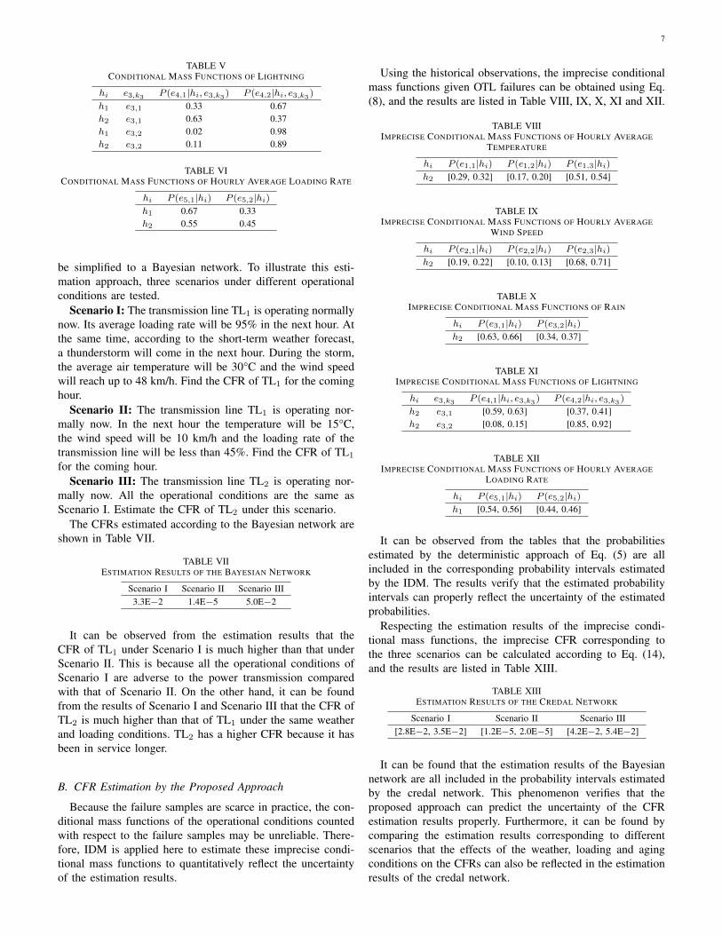
Moreover, to further test the proposed approach, the CFRsof TL2 in six successive time intervals were calculated. Thecorresponding operational conditions are listed in Table XIV.The estimation results are shown in Fig. 4.

VI. CONCLUSION

Because of the deficiency of the OTL failure samples, theCFR estimation result for the OTL may be unreliable in prac-tice. Under this circumstance, a novel imprecise probabilisticapproach for the CFR estimation, based on IDM and the credalnetwork, is proposed. According to this approach, the IDMis adopted to estimate the imprecise probabilistic dependencyrelations among the failure rate and the operational conditions,and the credal network is established to integrate the IDMestimation results and infer the imprecise CFR of the OTL.The proposed approach is tested by estimating the CFRs of

TABLE XIVOPERATIONAL CONDITIONS OF TL2 IN SUCCESSIVE TIME INTERVALS

Time Interval E1 E2 E3 E4 E5

1 e1,3 e2,2 e3,2 e4,2 e5,12 e1,3 e2,2 e3,2 e4,2 e5,23 e1,3 e2,3 e3,2 e4,2 e5,24 e1,3 e2,3 e3,2 e4,2 e5,15 e1,2 e2,3 e3,2 e4,2 e5,26 e1,2 e2,2 e3,1 e4,2 e5,2

Fig. 4. CFRs of TL2 in 6 successive time intervals.

two transmission lines located in the same region. The testresults illustrate that: a) the proposed approach can evaluatethe uncertainty of the CFR estimation result reasonably, b)the influences of the operational conditions on the CFR canbe reflected in the estimation result properly, and c) theuncertainty of the operational conditions can be handled bythe proposed approach conveniently.

REFERENCES

[1] R. Billinton and P. Wang, “Teaching distribution system reliabilityevaluation using Monte Carlo simulation,” IEEE Trans. Power Syst.,vol. 14, no. 2, pp. 397–403, 1999.

[2] D. Koval and A. Chowdhury, “Assessment of transmission-line common-mode, station-originated, and fault-type forced-outage rates,” IEEETrans. Ind. Appl., vol. 46, no. 1, pp. 313–318, Jan 2010.

[3] C. Williams, “Weather normalization of power system reliability in-dices,” in IEEE Power Eng. Soc. General Meeting. Tampa, FL, USA,2007, pp. 1–5.

[4] R. Billinton and G. Singh, “Application of adverse and extreme adverseweather: modelling in transmission and distribution system reliabilityevaluation,” Proc. Inst. Elect. Eng., Gen., Transm. Distrib., vol. 153,no. 1, pp. 115–120, 2006.

[5] R. Billinton and W. Li, “A novel method for incorporating weathereffects in composite system adequacy evaluation,” IEEE Trans. PowerSyst., vol. 6, no. 3, pp. 1154–1160, 1991.

[6] Y. Zhou, A. Pahwa, and S. S. Yang, “Modeling weather-related failuresof overhead distribution lines,” IEEE Trans. Power Syst., vol. 21, no. 4,pp. 1683–1690, 2006.

[7] W. Li, J. Zhou, and X. Xiong, “Fuzzy models of overhead power lineweather-related outages,” IEEE Trans. Power Syst., vol. 3, no. 23, pp.1529–1531, 2008.

[8] H. L. Willis, “Panel session on: aging t&d infrastructures and customerservice reliability,” in IEEE Power Eng. Soc. Summer Meeting, vol. 3.Seattle, WA, USA, 2000, pp. 1494–1496.

[9] P. Carer and C. Briend, “Weather impact on components reliability: Amodel for mv electrical networks,” in Proc. the 10th Int. Conf. PMAPS,.Rincon, Puerto Rico, USA, 2008, pp. 1–7.

[10] M. Bollen, “Effects of adverse weather and aging on power systemreliability,” IEEE Trans. Ind. Appl., vol. 37, no. 2, pp. 452–457, Mar2001.

[11] W. Christiaanse, “Reliability calculations including the effects of over-loads and maintenance,” IEEE Trans. Power Appa. & Syst., no. 4, pp.1664–1677, 1971.

[12] M. Finkelstein, Failure Rate Modelling for Reliability and Risk.Springer, 2008.

[13] P. Walley, Statistical Reasoning with Imprecise Probabilities. Chapman& Hall, 1991.

[14] J. M. Bernard, “An introduction to the imprecise Dirichlet model formultinomial data,” Int. J. Approx. Reason., vol. 39, no. 2, pp. 123–150,2005.

[15] A. R. Masegosa and S. Moral, “Imprecise probability models forlearning multinomial distributions from data. Applications to learningcredal networks,” Int. J. Approx. Reason., vol. 55, no. 7, pp. 1548–1569,2014.

[16] F. Coolen, “An imprecise Dirichlet model for Bayesian analysis of failuredata including right-censored observations,” Reliab. Eng. Syst. Safe.,vol. 56, no. 1, pp. 61–68, 1997.

[17] A. Antonucci, A. Piatti, and M. Zaffalon, “Credal networks for op-erational risk measurement and management,” in Knowledge-BasedIntelligent Information and Engineering Systems. Springer, 2007, pp.604–611.

[18] D. Heckerman, A Tutorial on Learning with Bayesian Networks.Springer, 1998.

[19] F. G. Cozman, “Credal networks,” Artif. Intell., vol. 120, no. 2, pp.199–233, 2000.

[20] F. G. Cozman, “Graphical models for imprecise probabilities,” Int. J.Approx. Reason., vol. 39, no. 2, pp. 167–184, 2005.

[21] J. Abellan and M. Gomez, “Measures of divergence on credal sets,”Fuzzy Set. Syst., vol. 157, no. 11, pp. 1514–1531, 2006.

[22] G. Corani, A. Antonucci, and M. Zaffalon, “Bayesian networks withimprecise probabilities: Theory and application to classification,” in DataMining: Foundations and Intelligent Paradigms. Springer, 2012, pp.49–93.