Interval Estimates for Predictive Values in Diagnostic Testing with

Interval Estimates for Predictive Values in Diagnostic Testing with Three Outcomes

Scott Clark, Lauren Mondin, Courtney Weber and Jessica Winborn

Advisor: Melinda Miller Holt

Abstract: In disease testing, patients and doctors are interested in estimates for positive

predictive value (PPV) and negative predictive value (NPV). The PPV of a test is the probability

that a patient actually has the disease, given a positive test result. The NPV is the probability that

a patient actually does not have the disease, given a negative test result. Here we consider

diagnostic tests in which the disease state remains uncertain, so the uncertain predictive value

(UPV) is also of interest. UPV is the probability that, given an uncertain test result, follow-up

testing will remain inconclusive. We derive classical Wald-type and Bayesian interval estimates

of PPV, NPV, and UPV. Performance of these intervals is compared through simulation studies

of interval coverage and width.

1. Introduction

The positive predictive value (PPV) and negative predictive value (NPV) of a diagnostic

test are important to both patients and doctors. The PPV of a test is the probability that, given a

positive test result, the patient actually has the disease. Similarly, the NPV of a test is the

probability that, given a negative test result, the patient is actually disease-free. Mercaldo et al.

(2007) derived Wald-type interval estimates of both PPV and NPV for binary diagnostic tests in

case-control studies where the true disease prevalence is assumed known. Stamey and Holt

(2010) derived analogous Bayesian interval estimates that allow for uncertainty relative to

disease prevalence. Here we consider studies in which both the diagnostic test under

consideration and the best test available may both provide inconclusive results, such as those

134Copyright © SIAM Unauthorized reproduction of this article is prohibited

reported in Khatami et al. (2007). We extend the results of Mercaldo et al. (2007) and Stamey

and Holt (2010) to diagnostic tests with three possible outcomes: positive, negative, and

uncertain. To address the possibility of inconclusive results, we derive an estimator for what we

call the uncertain predictive value (UPV). This is the probability that, given an uncertain initial

diagnostic result, the truth would remain unknown under the best test available, which we call

the “gold standard” for clarity. Because such follow-up procedures can be invasive and costly,

the UPV may be helpful in determining whether the patient should undergo more testing.

Other authors have considered similar situations, such as Feinstein (1990), which

considers a similar design with three results of the surrogate, or diagnostic, test but only two for

the gold standard test. As far as we know, there is no other work associated with three possible

outcomes for both the diagnostic test and the gold standard, as experienced by Khatami et al.

(2007).

To begin, Section 2 describes the experimental design and associated estimators

developed by Mercaldo et al. (2007) and Stamey and Holt (2010). Wald-type interval estimators

for PPV, NPV, and UPV are derived under an expanded design in Section 3.1. Section 3.2

presents analogous Bayesian interval estimators. In Section 4, we provide a performance analysis

comparing coverage and width of these intervals. Conclusions are offered in Section 5.

2. Binary Response Studies

2.1 Design

Consider first the study design described in Table 1. Let i = 1 represent the existence of

disease and i = 2 represent absence of disease. Similarly, let j = 1 represent a positive test result

and j = 2 represent a negative result. Thus xij represents the number of patients in disease state i


and test result j. Likewise ni represents the total number of people in disease state i. Mercaldo et

al. (2007) and Stamey and Holt (2010) described studies of this type that were not designed to

reflect the true disease prevalence in the target population. The same situation is considered here.

Thus, we assume that these values are available from sources external to the current study and

that p1 represents the known population probability of disease and p2 = 1 − p1 reflects the known

probability that a person is disease-free.

Test + Test − Total

Disease + x11 x12 n1 Disease − x21 x22 n2

Table 1: Binary Response Study Design

For such studies, researchers and clinicians are interested in estimating the sensitivity

(Se) of the test,

Se (Test | Disease )P= + +

and the specificity (Sp),

Sp (Test | Disease )P= − − .

Through Bayes Theorem, the sensitivity and specificity then lead to evaluation of the positive

predictive value

1

1 2

SePPV = (Disease | Test )Se (1 Sp)

pPp p

⋅+ + =

⋅ + −

and the negative predictive value

2

2 1

SpNPV (Disease | Test )Sp (1 Se)

pPp p

⋅= − − =

⋅ + −.

The data in Table 1 yield the following maximum likelihood estimators (MLE):

11

1

Se xn

= and 22

2

Sp xn

= .


Similarly, the false positive (Fp) and false negative (Fn) rates are estimated by

21

2

Fp xn

= and 12

1

Fn xn

= .

Based on the known prevalence values and the estimators above, estimators for the PPV and

NPV become

1

1 2

SePPVSe Fpp

p p⋅

=⋅ + ⋅

(1)

2

1 2

SpNPVFn Spp

p p⋅

=⋅ + ⋅

. (2)

Mercaldo et al. (2007) derived Wald-type interval estimators for both PPV and NPV, based on

equations (1) and (2). Likewise, Stamey and Holt (2010) derived analogous Bayesian estimators.

These will be discussed in Sections 2.2 and 2.3, respectively.

2.2 Wald-Type Intervals

Mercaldo et al. (2007) developed Wald-type interval estimators for PPV and NPV by

employing the delta method to determine the variances of PPV and NPV. Assuming that the

responses follow a binomial distribution and based on the asymptotic normality of the MLEs, the

authors proposed an approximate interval for PPV of the form

( ) ( )1 /2PPV PPVz varα−± ,

where is the (1-α/2)th quantile of the standard normal distribution and (1 /2z α− )

( )( )

2 21 2 1 2

1 24

1 2

( ) Se Fn ( Se) Sp Fp4

Fp

PPFp

4VSe

p p p pn nvar

p p

⋅ ⋅ ⋅ ⋅ ⋅ ⋅ ⋅ ⋅+

+ +=

⋅ ⋅ ⋅.


Similary, the estimator for NPV was

( ) ( )1 /2NPV NPVz varα−±,

where is the (1-α/2)th quantile of the standard normal distribution and (1 /2z α− )

( )( )

2 21 2 1 2

1 24

1 2

( ) Se Fn ( Fn) Sp Fp4

Sp

NPFn

4VSp

p p p pn nvar

p p

⋅ ⋅ ⋅ ⋅ ⋅ ⋅ ⋅ ⋅+

+ +=

⋅ ⋅ ⋅.

Mercaldo et al. (2007) also proposed alternate intervals based on an Agresti-type

adjustment (Agresti and Caffo, 2000). Here the adjusted estimates of Se and Sp became

2

1

1

Se2Se

kn

n

⋅ +=

and

2

2

2

Sp2Sp ,

kn

n

⋅ +=

so that the adjusted PPV and adjusted NPV calculations become

1

1 2

SePPVSe Fpp

p p⋅

=⋅ + ⋅

(3)

and

2

1 2

SpNPV ,Fn Spp

p p⋅

=⋅ + ⋅

(4)

respectively.


Mercaldo et al. (2007) compared the performance of these proposed interval methods, as

well as intervals based on their logit transformations, using simulations of confidence interval

width and coverage probability. They concluded that, when it provided a solution, the unadjusted

logit transformation performed best. Otherwise, they recommended the adjusted standard

interval. Stamey and Holt (2010) found, however, that the logit transformed solution often does

not exist. Thus, the research herein focuses on adjusted standard Wald-type intervals.

2.3 Bayesian Intervals

Stamey and Holt (2010) derived Bayesian interval estimates of PPV and NPV for case-

control studies described in Table 1. Because such designs require a priori knowledge of disease

prevalence, the authors considered two Bayesian models: one that took disease prevalence to be

known and one that placed a prior distribution on prevalence.

Like Mercaldo et al. (2007), Stamey and Holt (2010) assumed binomial data so that

( )11 1~ ,x binomial n Se and ( )22 2~ ,x binomial n Sp .

They assumed conjugate beta priors so that

Se SeSe ~ ( , )beta α β and Sp SpSp ~ ( , )beta α β ,

which yielded posterior distributions for Se and Sp of

11 Se 1 11 SeSe | ~ ( , )beta x n xα β+ − +d and 22 Sp 2 22 SpSp | ~ ( , )beta x n xα β+ − +d , (5)

where 11 22 1 2( , , , )x x n n=d .

Taking p1 and p2 to be known, Monte Carlo sampling from the posteriors in (5) provided

estimates of Se and Sp. Plugging these values into equations (1) and (2) yielded estimates of the

posterior distribution for the unadjusted estimates of PPV and NPV. Adjusted estimates of PPV

and NPV were similarly obtained, using equations (3) and (4).


The second model assumed that p1 is in fact estimated from previous survey data or

expert opinion. In this case, the value of p1 in (1) and (2) follows the posterior distribution

1 11 | ~ ( , )p pp beta y n yα β+ − +d

where the data vector is now 11 22 1 2( , , , , , )x x y n n n=d and y represents the number of patients with

the disease in a previous survey of n patients. Here Se, Sp, and p1 (and thus p2) are each obtained

through Monte Carlo sampling in order to estimate PPV and NPV.

The authors compared the interval width and true coverage probability of both Bayesian

intervals to that of the adjusted standard interval and the unadjusted logit interval of Mercaldo et

al. (2007) through simulation studies. They found that the Bayesian intervals maintained

coverage close to the nominal level, while the adjusted Wald-type interval dipped far below

nominal for large values of Sp. Widths were generally comparable for the methods that assumed

known prevalence, with the exception of large values of Sp. In that case, the Bayesian interval

was wider because it maintained coverage closer to nominal. The Bayesian procedure that

assumed unknown prevalence produced intervals that were generally wider than the other

methods, but maintained coverage quite close to nominal for all parameter values.

3. Multinomial Response Studies

3.1 Design

Now consider studies with the design described below in Table 2. Patients either have the

disease, do not have the disease, or their true state remains inconclusive, as determined by a gold

standard test. The diagnostic test under consideration may return results that are positive,

negative, or uncertain. Let i = 1 represent the existence of disease, i = 2 represent absence of


disease, and i = 3 represent true uncertainty. Similarly, let j = 1 represent a positive test result, j =

2 represent a negative test result, and j = 3 represent an inconclusive test result. Thus xij

represents the number of patients in disease state i and test result j. Likewise ni represents the

total number of people in disease state i.

Test + Test − Test 0 Total Disease + x11 x12 x13 n1 Disease − x21 x22 x23 n2 Disease 0 x31 x32 x33 n3

Table 2. Multinomial Response Study Design

The data in Table 2 yield the following maximum likelihood estimators (MLE) of

sensitivity (Se), specificity (Sp), and uncertainty (U):

11

1

Se xn

= , 22

2

Sp xn

= , and 33

3

U xn

= .

Similarly, the false positive (Fp) and false negative (Fn) rates are

21

2

Fp xn

= and 12

1

Fn xn

= .

Using this design, we must also consider the probability of an uncertain test result among

patients with the disease (Yu), the probability of an uncertain test result among patients without

the disease (Nu), the probability of a positive test that cannot be confirmed or refuted by the gold

standard (U1), and the probability of a negative test that cannot be confirmed or refuted by the

gold standard (U2). These values are estimated by the following:

13

1

Yu xn

= , 23

2

Nu xn

= , 311

3

U xn

= , and 322

3

U xn

=


Again we assume that p1 represents the known population probability of disease; p2

reflects the known probability that a person is disease-free; and p3 is equal to the known

probability of undeterminable results. Just as Mercaldo et al. (2007) and Stamey and Holt (2010)

assumed a binomial distribution, we assume that 1 11 12 13( , , )x x x x= , 2 21 22 23( , , )x x x x= , and

3 31 32 33( , , )x x x x= are independent and follow a multinomial distribution. Thus, the probability

mass function for x1 is

( ) 1311 12111 12 13

11 12 13

!, , Se Fn Yu! ! !

xx xnf x x xx x x

= .

We let t1 = (Se, Fn, Yu), and write x1 ~ M (n1, t1). Similarly, t2 = (Fp, Sp, Nu) and t3 = (U1, U2,

U) so that x2 ~ M (n2, t2), and x3 ~ M (n3, t3).

Applying Bayes Theorem produces the following estimators for PPV, NPV, and UPV:

1

1 2 3

SePPVSe Fp U

pp p p

⋅=

1⋅ + ⋅ + ⋅ (6)

2

1 2 3

SpNPVFn Sp U

pp p p

⋅=

2⋅ + ⋅ + ⋅ (7)

1 2

3

3

UUPVYu Nu U

pp p p

⋅=

⋅ + ⋅ + ⋅ (8)

Based on the equations (6) through (8), we extend the results of Mercaldo et al. (2007) and

Stamey and Holt (2010) to situations in which both the diagnostic test being evaluated and the

gold standard produce inconclusive results.


3.2 Wald-type Intervals

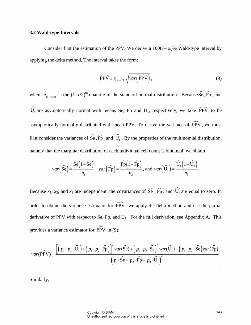
Consider first the estimation of the PPV. We derive a 100(1− α)% Wald-type interval by

applying the delta method. The interval takes the form:

( ) ( )1 /2PPV PPVz varα−± , (9)

where is the (1-α/2)th quantile of the standard normal distribution. Because , , and (1 /2z α− ) Se Fp

1U are asymptotically normal with means Se, Fp and U1, respectively, we take to be

asymptotically normally distributed with mean PPV. To derive the variance of , we must

first consider the variances of , , and

PPV

PPV

Se Fp 1U . By the properties of the multinomial distribution,

namely that the marginal distribution of each individual cell count is binomial, we obtain

( ) ( )1

Se 1 SeSevar

n

−= , ( ) ( )

2

Fp 1 FpFpvar

n

−= , and ( ) ( )1 1

13

U 1 UUvar

n

−= .

Because x1, x2, and x3 are independent, the covariances of , , and Se Fp 1U are equal to zero. In

order to obtain the variance estimator for , we apply the delta method and use the partial

derivative of PPV with respect to Se, Fp, and U1. For the full derivation, see Appendix A. This

provides a variance estimator for in (9):

PPV

PPV

( ) ( ) ( ) ( )( )

2 2

1 3 1 1 2 1 3 1 1 2

4

1 2 3 1

U Fp (Se) Se (U ) Se (Fp)(PPV)

Se Fp U

p p p p var p p var p p varvar

p p p

⎡ ⎤⋅ ⋅ + ⋅ ⋅ + ⋅ ⋅ + ⋅ ⋅⎣ ⎦=⋅ + ⋅ + ⋅

.

Similarly,


( ) ( )1

Sp 1 SpSpvar

n

−= , ( ) ( )

2

Fn 1 FnFnvar

n

−= , and ( ) ( )2 2

23

U 1 UUvar

n

−= ,

which lead to

( ) ( ) ( ) ( ) ( )( )

2 2

2 3 2 1 2 2 3 2

4

2 2 2

2

3

1U Fn (Sp) SNPV

Fn

p (U ) Sp (Fn

Sp U

p p p p var p p vvar

p p p

ar p p var⎡ ⎤⋅ ⋅ + ⋅ ⋅ + ⋅ ⋅ + ⋅ ⋅=

⋅ + ⋅ + ⋅

⎣ ⎦ )

and the interval estimator

( )(1 /2)NPV NPVz varα−± . (10)

Lastly,

( ) ( )1

Yu 1 YuYuvar

n

−= , ( ) ( )

2

Nu 1 NuNuvar

n

−= , and ( ) ( )

3

U 1 UUvar

n

−= ,

which lead to

( ) ( ) ( ) ( ) ( ) ( ) ( ) ( )( )

2 2 2

1 3 2 3 2 3 1 3

4

1 2 3

Yu Nu U U Nu U YuUPV

Yu Nu U

p p p p var p p var p p varvar

p p p

⎡ ⎤⋅ ⋅ + ⋅ ⋅ + ⋅ ⋅ + ⋅ ⋅⎣ ⎦=

⋅ + ⋅ + ⋅

and the interval estimator

( )(1 /2)UPV UPVz varα−± . (11)

As do Mercaldo et al. (2007), we consider an Agresti type adjustment (2000) to improve

performance of the estimators for proportions near 0 or 1. To do so, the data in Table 2 is

adapted to become those presented below in Table 3.


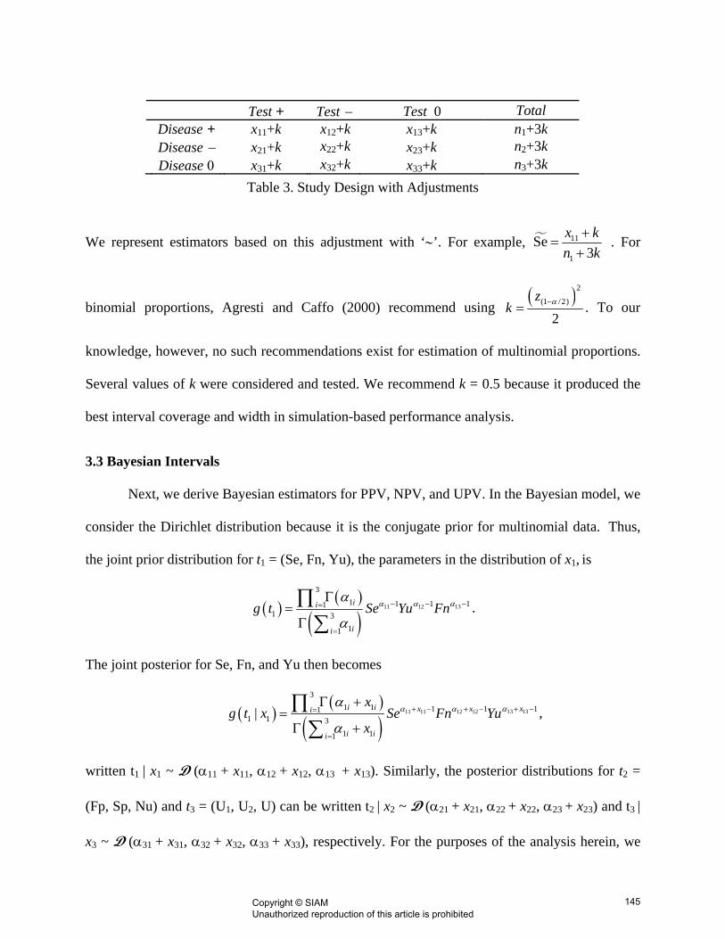
Test + Test − Test 0 Total Disease + x11+k x12+k x13+k n1+3k Disease − x21+k x22+k x23+k n2+3k Disease 0 x31+k x32+k x33+k n3+3k

Table 3. Study Design with Adjustments

We represent estimators based on this adjustment with ‘∼’. For example, 11

1

Se3

x kn k

+=

+ . For

binomial proportions, Agresti and Caffo (2000) recommend using ( )2

(1 /2)

2z

k α−= . To our

knowledge, however, no such recommendations exist for estimation of multinomial proportions.

Several values of k were considered and tested. We recommend k = 0.5 because it produced the

best interval coverage and width in simulation-based performance analysis.

3.3 Bayesian Intervals

Next, we derive Bayesian estimators for PPV, NPV, and UPV. In the Bayesian model, we

consider the Dirichlet distribution because it is the conjugate prior for multinomial data. Thus,

the joint prior distribution for t1 = (Se, Fn, Yu), the parameters in the distribution of x1, is

( )( )

( )1311 12

31 1

13

1111

1

ii

ii

g t Se Yu Fn −− −=

=

Γ=

Γ

∏∑

αα αα

α.

The joint posterior for Se, Fn, and Yu then becomes

( )( )

( )13 1311 1 1211 2

31 1 11 11

1 1 31 11

| i i xx xi

i ii

xg t x Se Fn Yu

x+ −+ − + −=

=

Γ +=

Γ +

∏∑

αα αα

α,

written t1 | x1 ~ D (α11 + x11, α12 + x12, α13 + x13). Similarly, the posterior distributions for t2 =

(Fp, Sp, Nu) and t3 = (U1, U2, U) can be written t2 | x2 ~ D (α21 + x21, α22 + x22, α23 + x23) and t3 |

x3 ~ D (α31 + x31, α32 + x32, α33 + x33), respectively. For the purposes of the analysis herein, we


consider noninformative Dirichlet priors with parameter values equal to 0.5. This makes the

Bayesian analysis analogous to the Wald-type analysis in that no information is available relative

to t1, t2, and t3 beyond that in Table 3.

Here again, the prevalence vector, p = (p1, p2, p3), is assumed known, so the posterior

distributions for PPV, NPV, and UPV can be approximated via Monte Carlo sampling by B

values from the posteriors of t1, t2, and t3. At each iteration, the generated values of Se(j), Fn(j),

Yu(j), Fp(j), Sp(j), Nu(j), U1(j), U2

(j), and U(j) are plugged into

( )( ) 1

( ) ( ) ( )1 2 3

SePPVSe Fp U

jj

1j j

pp p p

⋅=

⋅ + ⋅ + ⋅ j , (12)

( )

( ) 2( ) ( ) ( )

1 2 3

SpNPVFn Sp U

jj

2j j j

pp p p

⋅=

⋅ + ⋅ + ⋅ , (13)

and

( )( )

( ) ( ) ( )1

3

2 3

UUPVYu Nu U

jj

j j

pp p p

⋅=

⋅ + ⋅ + ⋅ j , (14)

where the superscript (j) denotes that this is the jth iteration in the Monte Carlo approximation.

The posteriors for PPV, NPV, and UPV are then approximated using these B values. The 2.5th

and 95.5th percentiles of the distribution then provide the 95% Bayesian credible sets.

4. Performance Analysis

This section provides a simulation-based comparison of the 95% adjusted Wald-type and

Bayesian interval estimates of PPV through both coverage probability and interval width.

Consider n1 = n2 = n3 = 25, Sp = 0.5, and let Se vary from 0.5 to 0.80 by 0.10. For this analysis,

Yu = Nu = 0.1, U1 = 0.8, U = U2 = 0.1, Fp = 0.4, and Fn varies with Se. In each boxplot, values


of p1 vary from 0.50 to 0.85 by 0.05, while fixing p3 = 0.10 so that p2 varies from 0.05 to 0.40 by

0.05. For each set of parameter values, 10,000 samples were simulated leading to 10,000 Wald

(W) and Bayesian (B) intervals. Coverage probability and width are estimated by averaging over

the 10,000 samples. Figure 1 compares resulting estimates of coverage probability, while Figure

2 compares interval width.

Figure 1. PPV Coverage Probability Comparison for Sp = 0.5, Se = 0.5, 0.6, 0.7, 0.8

Figure 2. PPV Width Comparison for Sp = 0.5, Se = 0.5, 0.6, 0.7, 0.8


Figure 1 indicates that the Bayesian coverage probability remains closer to the nominal

0.95 when estimating PPV than that of the Wald-type interval for the parameters considered

here, while Figure 2 suggests that the Bayesian interval is slightly narrower. Figures 3 and 4

provide the coverage and width, respectively, for estimating NPV at the same parameter values.

These plots indicate generally the same performance pattern, with the Bayesian interval coverage

closer to nominal and its width narrower. The behavior exhibited here by the Wald-type intervals

is similar to that observed in Stamey and Holt (2010), because coverage deviates further from

nominal as Se increases. Likewise, the width of the Bayesian interval increases, while coverage

remains close to nominal.

Figure 3. NPV Coverage Probability Comparison for Sp = 0.5, Se = 0.5, 0.6, 0.7, 0.8


Figure 4. NPV Width Comparison for Sp = 0.5, Se = 0.5, 0.6, 0.7, 0.8

Figures 5 and 6 below indicate that the Bayesian coverage probabilities are much closer

to nominal than those of the Wald-type interval when estimating UPV, although generally the

Bayesian interval is slightly wider.

Figure 5. UPV Coverage Probability Comparison for Sp = 0.5, Se = 0.5, 0.6, 0.7, 0.8


Figure 6. UPV Width Comparison for Sp = 0.5, Se = 0.5, 0.6, 0.7, 0.8

Several other sets of parameter values were considered, varying Sp and sample size.

Those simulation results are not included for the sake of space. For varying values of Sp the

behavior demonstrated above remains consistent. At sample sizes of 50 and above, the two

procedures maintained very similar coverage and width. Further details about simulation results

are available from the authors.

5. Example

The research herein was motivated by the work of Khatami et al. (2007). Khatami and

co-authors developed a prediction model, combining the results of various blood and tissue

markers, to determine whether or not a cancer originated in the ovaries. The model designated

the cancer origin as ovaries, not ovaries, or uncertain. To determine its effectiveness, they

compared its diagnoses against the standard histologic assessment. Table 4 describes the data

obtained in their experiment:


Test + Test - Test 0 Total Disease + 118 6 6 130 Disease - 6 15 11 32 Disease 0 23 4 9 36

Table 4. Ovarian Cancer Data (Khatami et al., 2007)

In order to calculate the interval estimates of PPV, NPV, and UPV, the values of p1, p2, and p3

must be determined. We take these to be known but base them on calculations in Khatami et al.

(2007), we take p1 to be 0.66. We take p2 and p3 to be 0.16 and 0.18, respectively. For the

adjusted Wald-type interval, we take a = 0.5. For the Bayesian credible sets, t1, t2, and t3 are each

given noninformative Dirichlet (0.5, 0.5, 0.5) distributions. The resulting interval estimates are

presented in Table 5.

Table 5. Interval Estimates of PPV, NPV and UPV from Khatami et al. (2007)

Method PPV

Estimate 95%

Interval NPV

Estimate95%

Interval UPV

Estimate 95%

Interval Wald 0.805 0.767-0.844 0.599 0.435-0.770 0.345 0.187-0.505

Adjusted Wald 0.805 0.768-0.847 0.599 0.415-0.748 0.345 0.186-0.499 Bayes 0.801 0.779-0.823 0.595 0.473-0.717 0.302 0.216-0.398

Evaluating Table 5, we see that the interval estimates are very similar. The main difference is in

the different interpretations of a confidence interval and a credible set. A confidence interval

states that there is a 95% chance that the true proportion is in the interval, while the credible set

states that if we run the test an infinite number of times, 95% of the time the true proportion will

be in the interval.


6. Conclusion

In this paper, we derive both Wald-type and Bayesian interval estimates of PPV, NPV,

and UPV for diagnostic procedures with three possible outcomes. We considered prevalence to

be known for both the Wald-type and Bayesian analysis. Both of these methods require

knowledge of the outcome of the gold standard. Simulation studies indicate that the Bayesian

approach using noninformative priors typically provides better coverage and smaller width than

that of the Wald-type interval with a 0.5 Agresti type adjustment. It is, therefore, our conclusion

that the Bayesian method is preferred. Future research will consider Bayesian analyses that

incorporate informative Dirichlet priors to reflect any available prior information on values such

as the sensitivity and specificity in order to further improve performance of the Bayesian method

and Bayesian methods for estimating PPV, NPV, and UPV for unknown prevalence. Additional

work will also expand the second model in Stamey and Holt (2010) to account for possible

uncertainty about disease prevalence values.

ACKNOWLEDGEMENTS

We wish to thank the anonymous referees for their comments that significantly improved the

paper. Also, we wish to thank Dr. Ken Smith and the National Science Foundation for their

support through grant #DMS-0636528.


References:

Agresti, A. and Caffo, B. (2000). “Simple and Effective Confidence Intervals for Proportions and Differences of Proportions.” The American Statistician 54: 20-88. Feinstein, A. (1990). “The Inadequacy of Binary Models for the Clinical Reality of Three-Zone Diagnostic Decisions.” J Clin Epidemiol 43: 109-113. Khatami, Z. Cross P., Stevenson M.R., Naik R. (2007). “Design of a bio-mathematical prediction model using serum tumor markers and immunohistochemistry in peritoneal carcinomatosis with ovarian involvement: a pilot study.” International Journal of Gynecological Cancer 17:1258-1263.

Mercaldo, N. D. Lau, K. G., Zhou, X. H. (2007). “Confidence Intervals for predictive values with an emphasis to case-control studies.” Statistics in Medicine 26:2170-2183.

Stamey, J. Holt, M. A. (2010) “Bayesian interval estimation for predictive values from case-control studies.” Communications in Statistics - Simulation and Computation 39: 101-110.


Appendix A

To derive var(PPV) we employ the delta method, so that ,

where

(PPV) = ( PPV)' ( PPV)var ∇ Σ ∇

[ ]1PPV (PPV) (Se), (PPV) (U ), (PPV) (Fp)∇ = ∂ ∂ ∂ ∂ ∂ ∂ and Σ is the variance/covariance

matrix of v = (Se, U1, Fp). Recall that

( ) ( ) ( )1

1 2 3

SePPVSe Fp U

pp p p 1

⋅=

⋅ + ⋅ + ⋅.

Thus,

( )1

1 1

(PPV) (PPV)(Se) (Se)(Se) 0 0

(PPV) (PPV)PPV 0 (Fp) 0(Fp) (Fp)

0 0 (U )(PPV) (PPV)(U ) (U )

T

varvar var

var

⎡ ⎤ ⎡ ⎤∂ ∂⎢ ⎥ ⎢ ⎥∂ ∂⎢ ⎥ ⎢ ⎥⎡ ⎤⎢ ⎥ ⎢ ⎥∂ ∂⎢ ⎥= ⎢ ⎥ ⎢ ⎥⎢ ⎥∂ ∂⎢ ⎥ ⎢ ⎥⎢ ⎥⎣ ⎦⎢ ⎥ ⎢ ⎥∂ ∂⎢ ⎥ ⎢ ⎥∂ ∂⎣ ⎦ ⎣ ⎦

( ) ( )( ) ( ) ( ) ( ) ( ) ( ) ( ) ( ) ( )

1 2 1 3 1 1 31 22 2

1 2 3 1 1 2 3 1 1 2 3 1

Fp U SeSeSe Fp U Se Fp U Se Fp U

p p p p p pp pp p p p p p p p p

⎡ ⎤⋅ ⋅ + ⋅ ⋅ − ⋅ ⋅− ⋅ ⋅⎢ ⎥=⎢ ⎥⋅ + ⋅ + ⋅ ⋅ + ⋅ + ⋅ ⋅ + ⋅ + ⋅⎡ ⎤ ⎡ ⎤ ⎡ ⎤⎣ ⎦ ⎣ ⎦ ⎣ ⎦⎣ ⎦

2

( )

( )

( )

( ) ( )( ) ( ) ( )

( ) ( ) ( )

( ) ( ) ( )

1 2 1 3 12

1 2 3 11

1 22

2 1 2 3 1

1 1 1 32

31 2 3 1

Fp USe 1 Se0 0

Se Fp UFp 1 Fp Se0 0

Se Fp UU 1 U Se0 0

Se Fp U

p p p p

p p pn

p pn p p p

p pn p p p

⎡ ⎤⋅ ⋅ + ⋅ ⋅−⎡ ⎤ ⎢ ⎥⎢ ⎥ ⎢ ⎥⋅ + ⋅ + ⋅⎡ ⎤⎣ ⎦⎢ ⎥ ⎢ ⎥⎢ ⎥− − ⋅ ⋅⎢ ⎥⎢ ⎥ ⎢ ⎥⎢ ⎥ ⋅ + ⋅ + ⋅⎡ ⎤⎣ ⎦⎢ ⎥⎢ ⎥ ⎢ ⎥− − ⋅ ⋅⎢ ⎥ ⎢ ⎥⎢ ⎥⎣ ⎦ ⎢ ⎥⋅ + ⋅ + ⋅⎡ ⎤⎣ ⎦⎣ ⎦


( ) ( ) ( ) ( ) ( ) ( ) ( )

( ) ( ) ( )

2 2 2 1 11 2 1 3 1 1 2 1 3

1 24

1 2 3 1

Se 1 Se Fp 1 Fp U 1 UFp U Se Se

.Se Fp U

p p p p p p p pn n

p p p

− −⎛ ⎞ ⎛ ⎞ ⎛⋅ ⋅ + ⋅ ⋅ + − ⋅ ⋅ + − ⋅ ⋅⎡ ⎤ ⎜ ⎟ ⎜ ⎟ ⎜⎣ ⎦

⎝ ⎠ ⎝ ⎠ ⎝=⋅ + ⋅ + ⋅⎡ ⎤⎣ ⎦

3n− ⎞

⎟⎠

Substituting the estimators , , and Se Fp 1U , yields the estimator for ( )PPV .var The values of

( )UPVvar and are derived using the same method and thus omitted. (NPVvar )


Documents

Interval Estimates for Predictive Values in Diagnostic Testing with