Embed Size (px)
Citation preview
2006.11.21
Interval-Based Hybrid Dynamical Systemfor Modeling Dynamic Events g yand Structures
Hiroaki KawashimaHiroaki Kawashima
2007.2.7
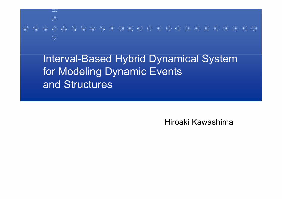
Event Recognitiong
Sensor (ex. camera, microphone)
Real world
Time-varying signals
Feature Extraction(signal processing)(signal processing)
D namic Feat re Seq ence of Static or D namic Feat reDynamic Feature Sequence of Static or Dynamic Feature
Static Pattern Recognition(ex Nearest Neighbor)
Trajectory Matching(ex DP matching method)
State-Transition Model (ex. HMM, Dynamical System,(ex. Nearest Neighbor) (ex. DP matching method) ( y y
Automaton)
2007.2.7
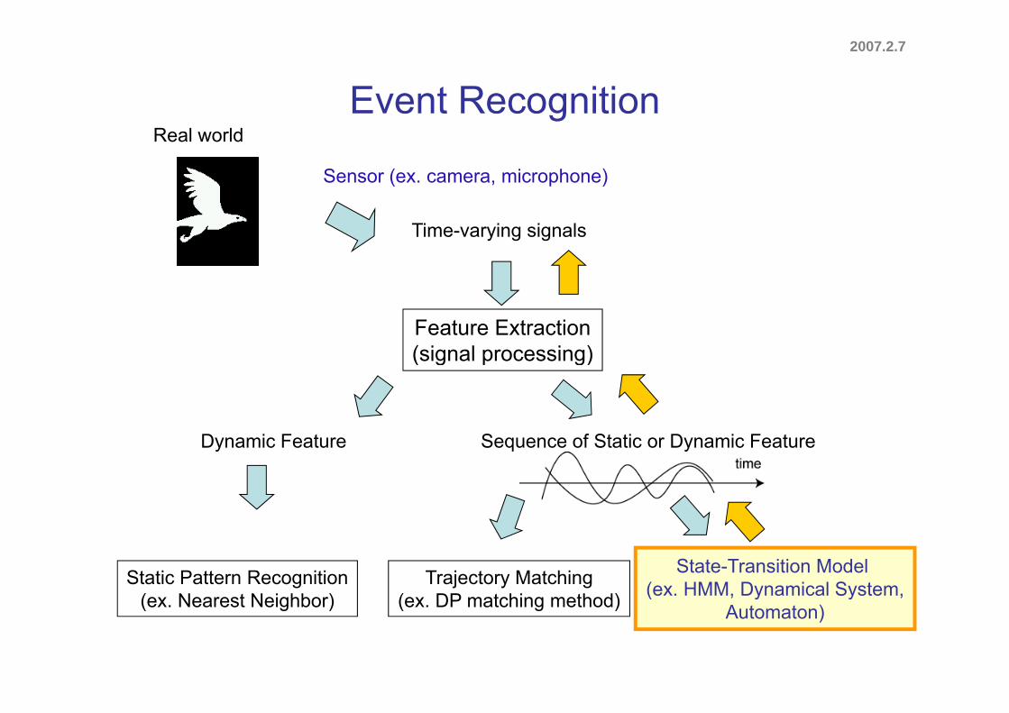
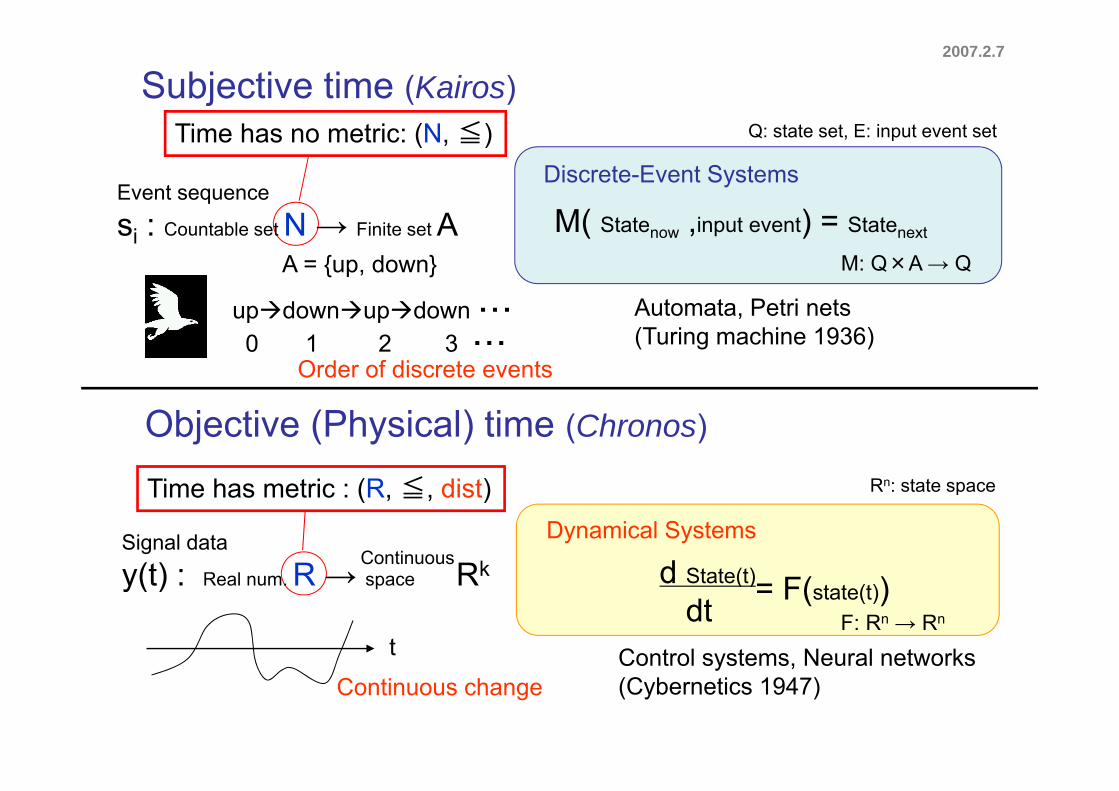
T C t f TiTwo Concepts of Time
Time flies faster than it
used to…
?
2007.2.7
Subjective time (Kairos)Ti h t i (N ≦) Q t t t E i t t t
Discrete-Event Systems
M( ) =
Time has no metric: (N, ≦)
Event sequence
N A
Q: state set, E: input event set
M( Statenow ,input event) = Statenext
M: Q×A → Q
Automata Petri nets
si : Countable set N → Finite set AA = {up, down}
pdo n pdo n Automata, Petri nets(Turing machine 1936)
updownupdown ・・・
0 1 2 3 ・・・Order of discrete events
Objective (Physical) time (Chronos)
Time has metric : (R ≦ dist) Rn: state space
d State(t)
Dynamical Systems
Time has metric : (R, ≦, dist)
Signal data
y(t) : R l R → RkContinuous
Rn: state space
d State(t)
dt= F(state(t))
F: Rn → Rn
Control systems, Neural networkst
y(t) : Real num. R → space Rk
Control systems, Neural networks(Cybernetics 1947)Continuous change
2007.2.7
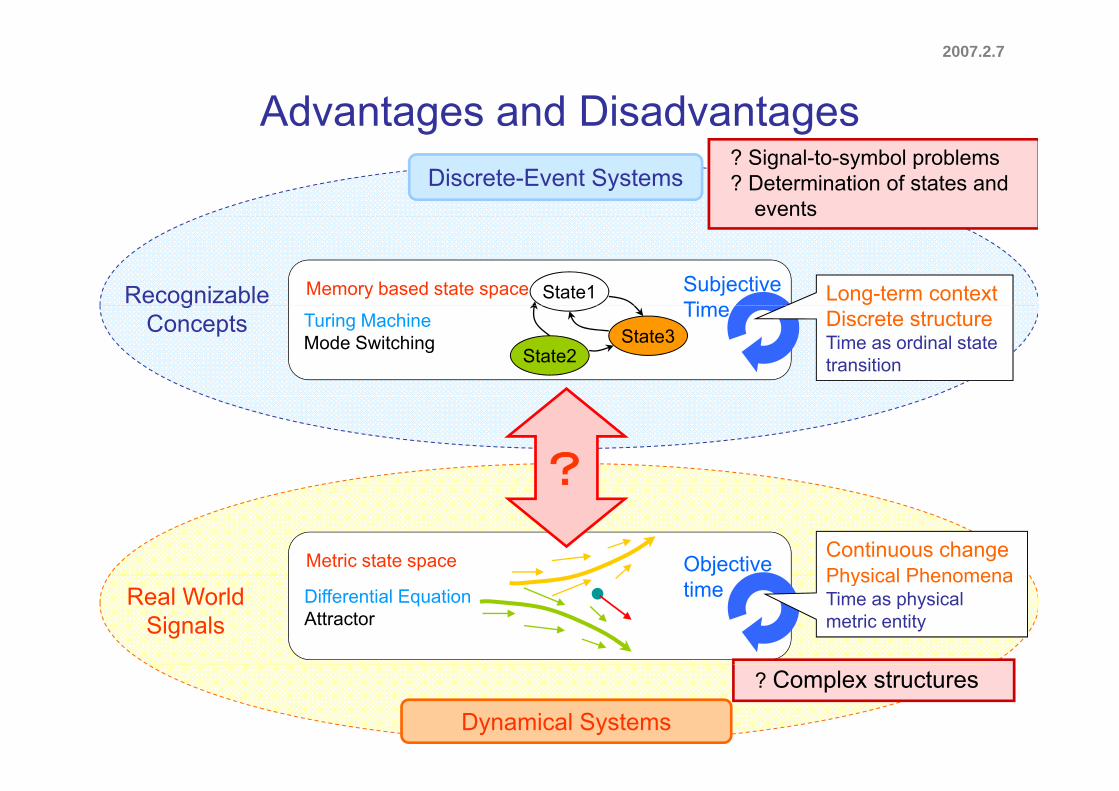
Advantages and DisadvantagesDiscrete-Event Systems
? Signal-to-symbol problems? Determination of states and
events
g g
Recognizable Memory based state space State1 SubjectiveTime
Long-term context
e e s
gConcepts Turing Machine
Mode SwitchingState2
State3Time Discrete structure
Time as ordinal state transition
?
Metric state space ObjectiveContinuous changePhysical Phenomena
Real World Signals
Differential EquationAttractor
jtime
Physical PhenomenaTime as physical metric entity
Dynamical Systems
? Complex structures
2007.2.7
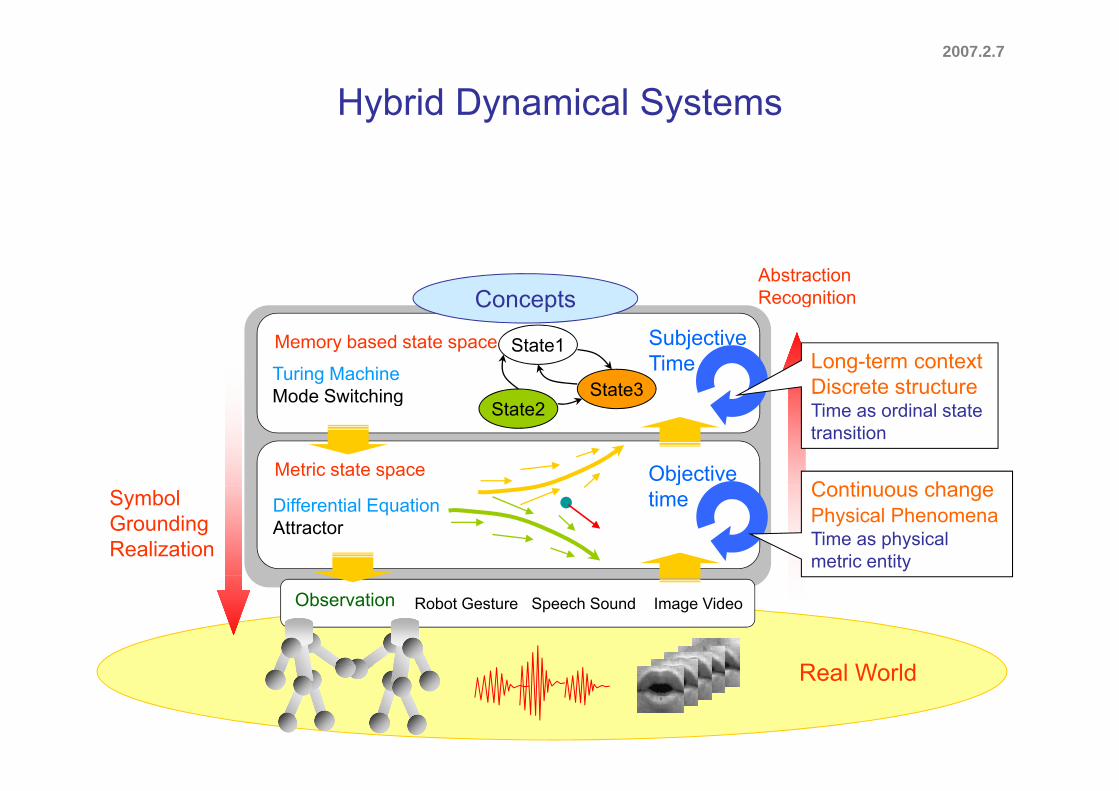
Hybrid Dynamical Systems
AbstractionRecognitionConcepts g
Turing MachineMode Switching
Memory based state space State1
State3
SubjectiveTime
Concepts
Long-term contextDiscrete structure
Metric state space
Mode SwitchingState2
State3
Objective
Time as ordinal state transition
Contin o s changeDifferential EquationAttractor
timeSymbol GroundingRealization
Continuous changePhysical PhenomenaTime as physical metric entity
Robot Gesture Speech Sound Image VideoObservation
R l W ldReal World
2007.2.7
Existing Studies• Computer vision
– Hybrid dynamical models [C. Bregrler 1997]– Multi-class condensation [B North A Blake M Isard and J Rittscher 2000]
g
Multi-class condensation [B. North, A. Blake, M. Isard and J. Rittscher, 2000]– Switching linear dynamical systems [K.P. Murphy 1998, V. Pavlovic 1999]
• Speech recognition– Segment models [M. Ostendorf 1996]
• Computer graphicsM ti t t [Y Li T W H Y Sh 2002]– Motion textures [Y. Li, T. Wang, H.Y. Shum 2002]
• Neural networks, Control theory, etc.Piecewise linear models [R Batruni 1991]– Piecewise linear models [R. Batruni 1991]
– Switching space models [Z. Ghahramani 1996]– Piecewise affine maps [L. Breiman 1993]
– Hybridautomata [R. Alur 1993]
Integration of “subjective time” and “objective time”?
2007.2.7
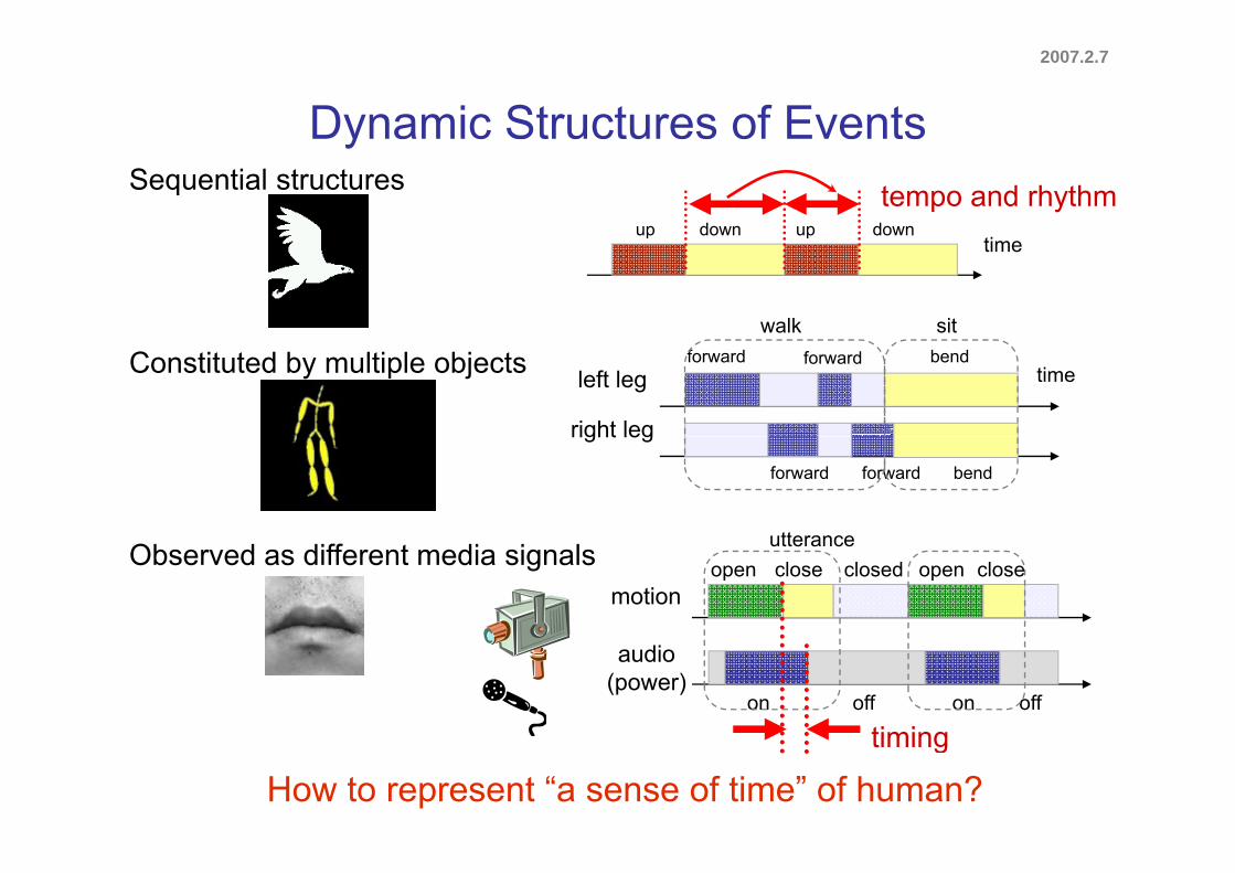
Dynamic Structures of EventsySequential structures
tiup down downup
tempo and rhythmtime
p p
walk sit
Constituted by multiple objects left leg
right leg
timeforward forward bend
right leg
forward forward bend
utteranceObserved as different media signals open close closeopenclosedmotion
utterance
audio(power)
on off on off
timing
How to represent “a sense of time” of human?timing
2007.2.7
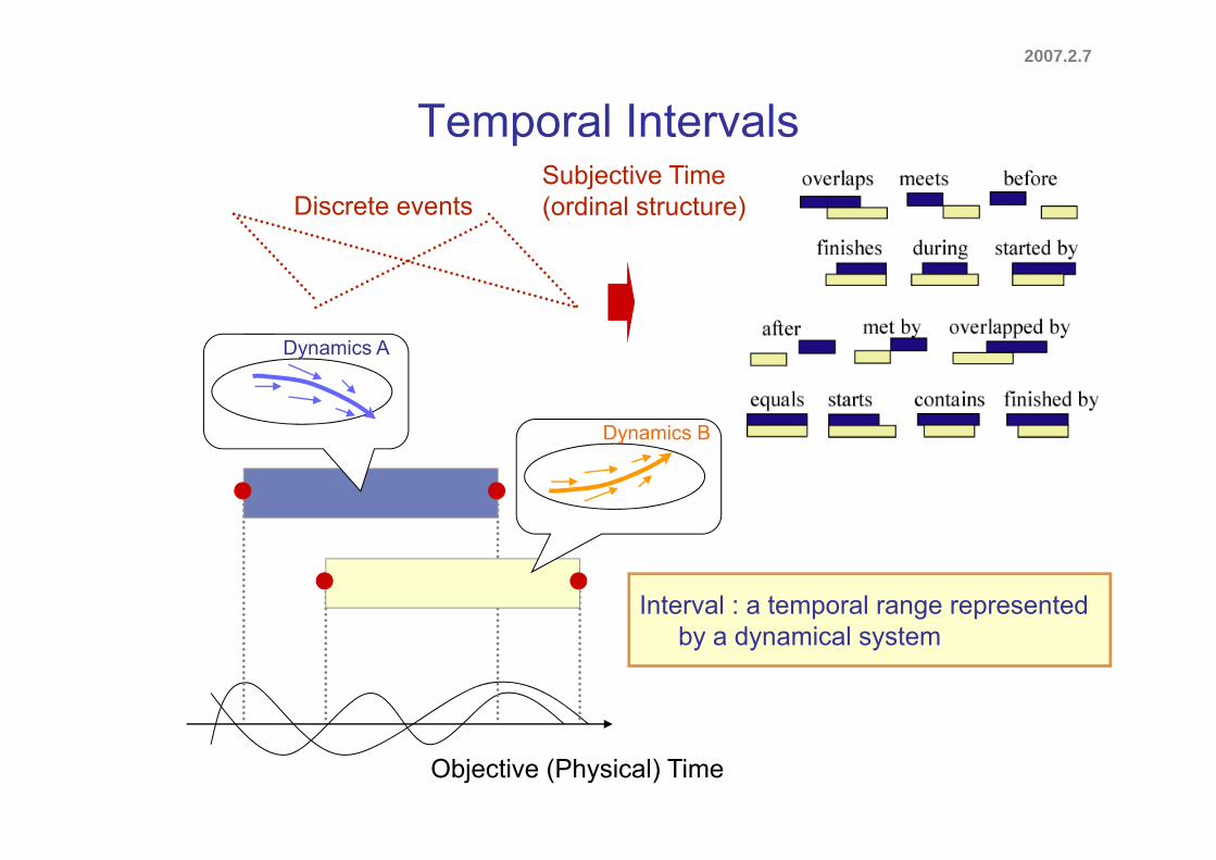
Temporal Intervalsp
Discrete eventsSubjective Time(ordinal structure)
Dynamics A
Dynamics BDynamics B
Interval : a temporal range represented by a dynamical system
Objective (Physical) Time
2007.2.7
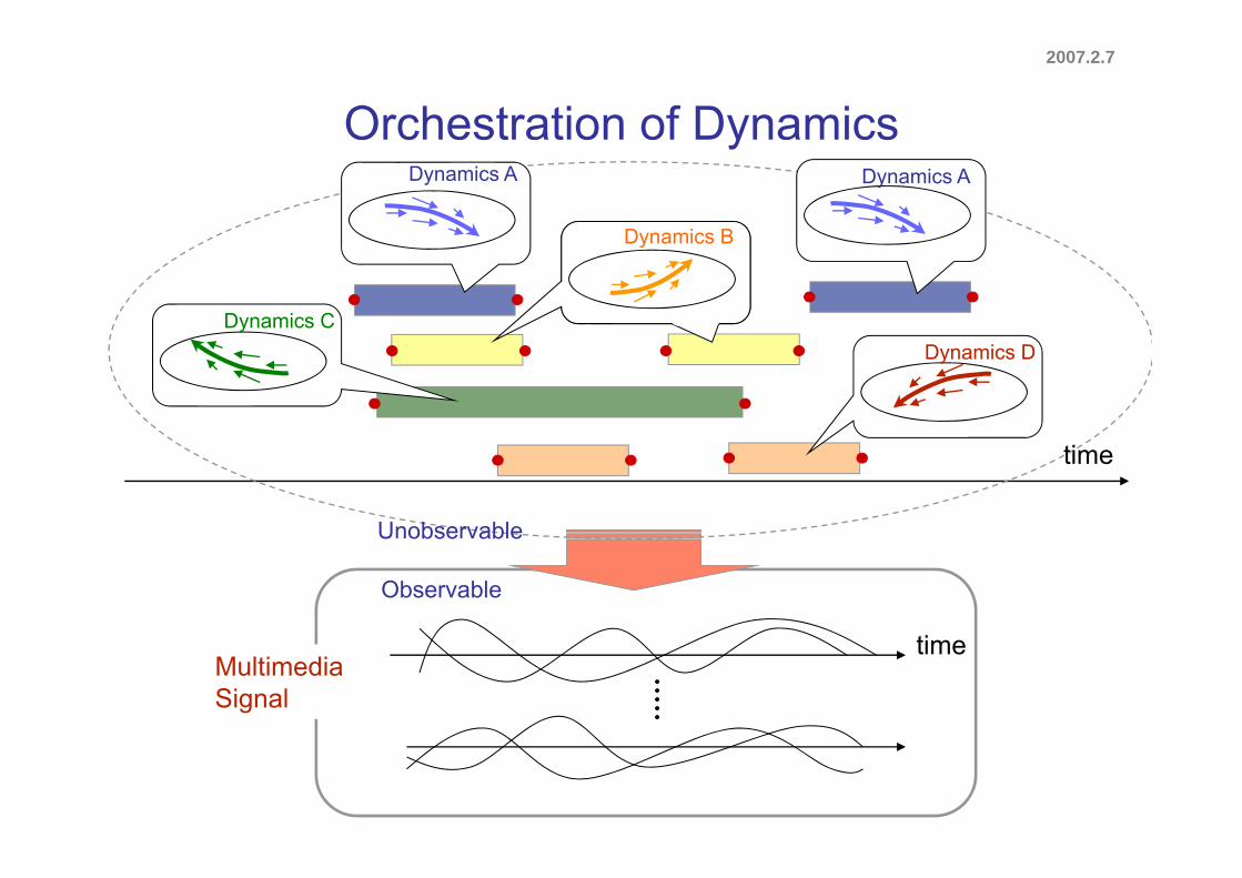
Orchestration of DynamicsyDynamics A Dynamics A
Dynamics B
Dynamics C
Dynamics B
Dynamics D
Unobservable
time
ti
Observable
U obse ab e
timeMultimediaSignal
2007.2.7
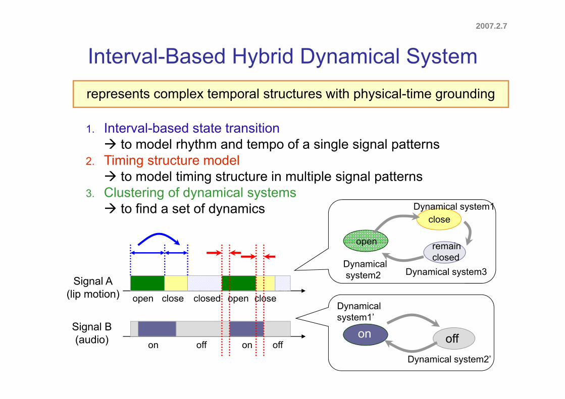
Interval-Based Hybrid Dynamical Systemy y yrepresents complex temporal structures with physical-time grounding
1. Interval-based state transition to model rhythm and tempo of a single signal patterns
2. Timing structure model to model timing structure in multiple signal patterns
3. Clustering of dynamical systems
remainopen
close
g y y to find a set of dynamics Dynamical system1
Signal A(li ti )
remainclosed
p
Dynamicalsystem2 Dynamical system3
open close closeopenclosed(lip motion)
Signal B( ) ffon
Dynamical system1’
(audio) on off on off offon
Dynamical system2’
2007.2.7
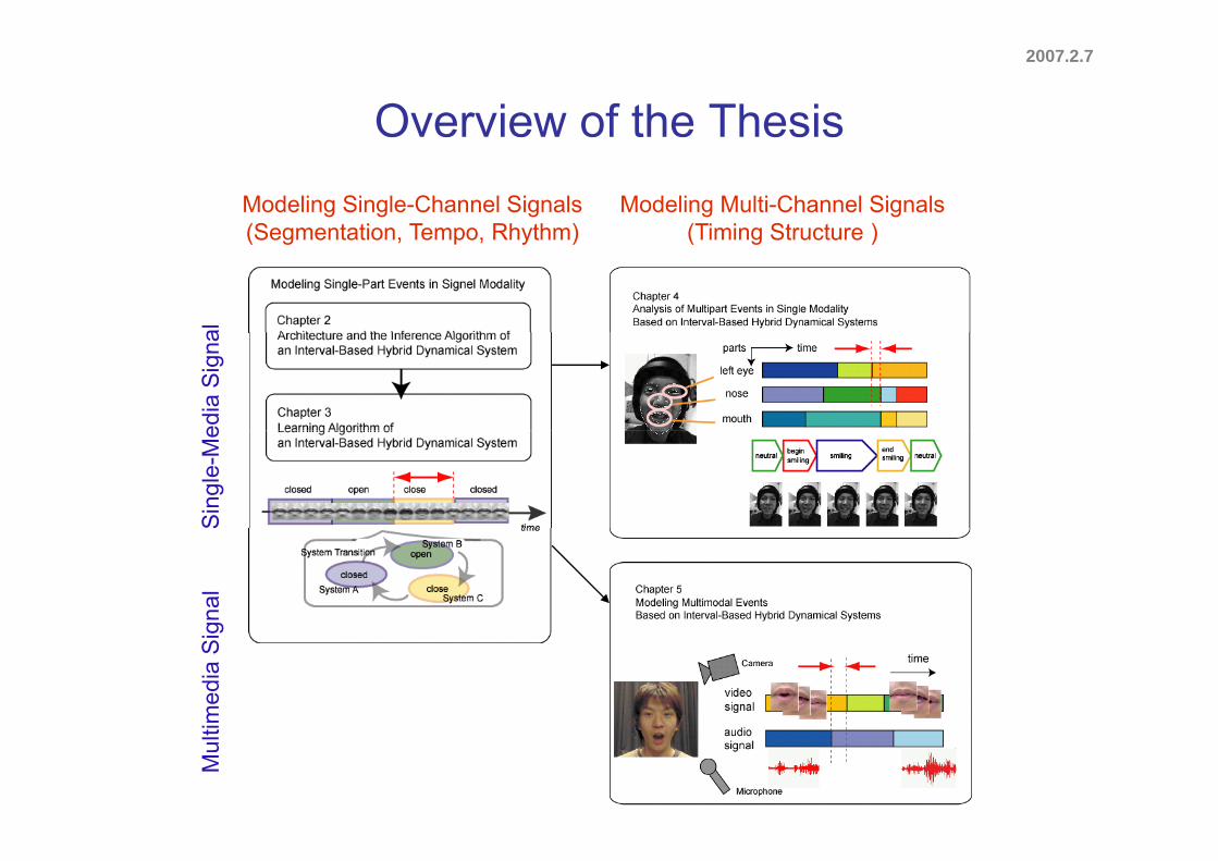
Overview of the ThesisModeling Single-Channel Signals(Segmentation Tempo Rhythm)
Modeling Multi-Channel Signals(Timing Structure )(Segmentation, Tempo, Rhythm) (Timing Structure )
aled
ia S
igna
Sin
gle-
Me
gnal
med
ia S
igM
ulti
2006.11.21
Chapter 2
Interval-Based Hybrid Dynamical Systemy y y
2007.2.7
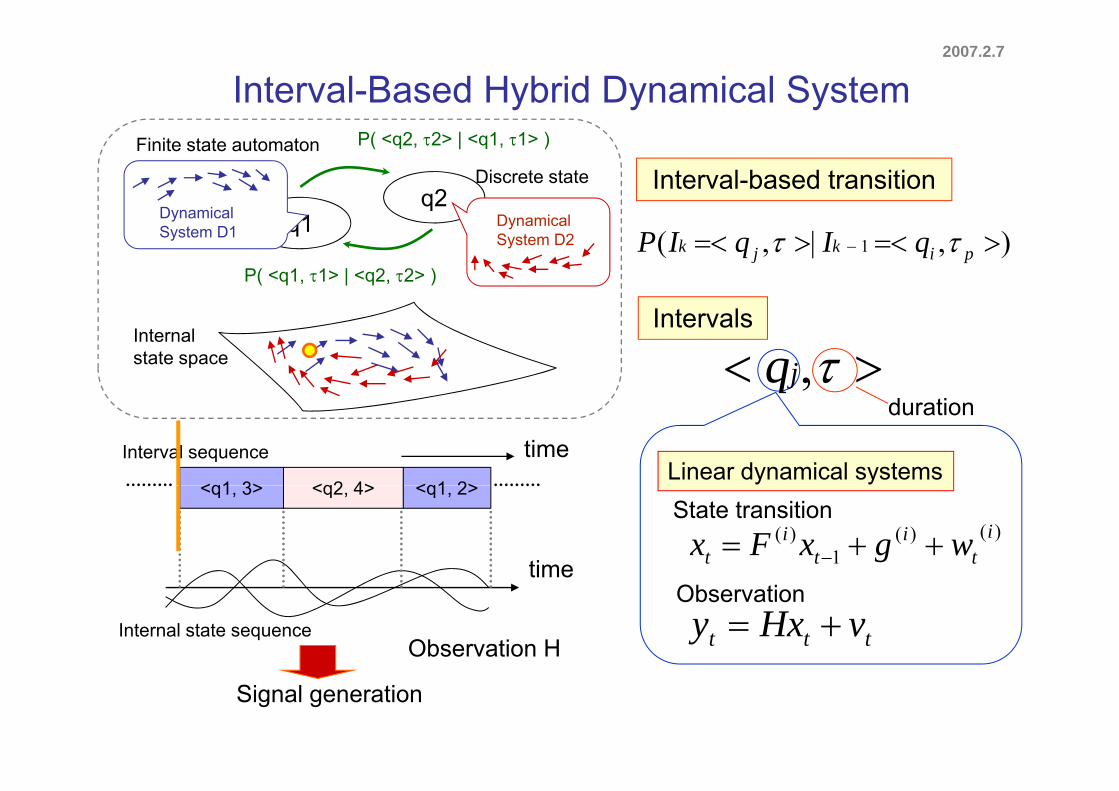
Interval-Based Hybrid Dynamical System
1q2
Finite state automaton P( <q2, 2> | <q1, 1> )
D i lDynamical
Interval-based transitionDiscrete state
),|,( 1 pikjk qIqIP q1
P( <q1, 1> | <q2, 2> )
DynamicalSystem D2
DynamicalSystem D1
,jqIntervals
Internalstate space
Linear dynamical systems
duration
time<q1 3> <q1 2><q2 4>
Interval sequence
)()(1
)( it
it
it wgxFx
State transition<q1, 3> <q1, 2><q2, 4>
time
ttt vHxy Observation
time
Internal state sequenceObservation H
Signal generation
2007.2.7
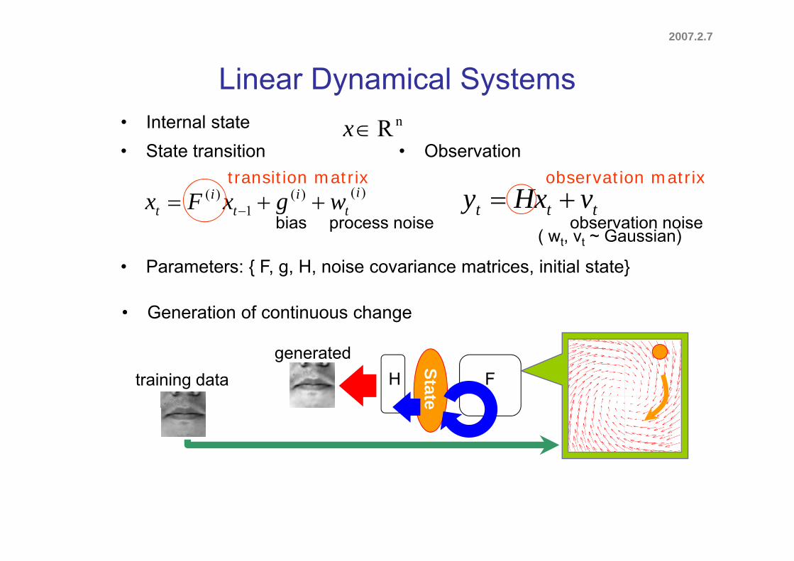
Linear Dynamical Systems• Internal state nRx• State transition • Observation
y y
)()(1
)( it
it
it wgxFx
State transition
ttt vHxy
Observationtransition matrix observation matrix
bi i b ti i
• Parameters: { F, g, H, noise covariance matrices, initial state}
bias process noise observation noise( wt, vt ~ Gaussian)
• Generation of continuous change
FHState
generatedtraining data
e
2007.2.7
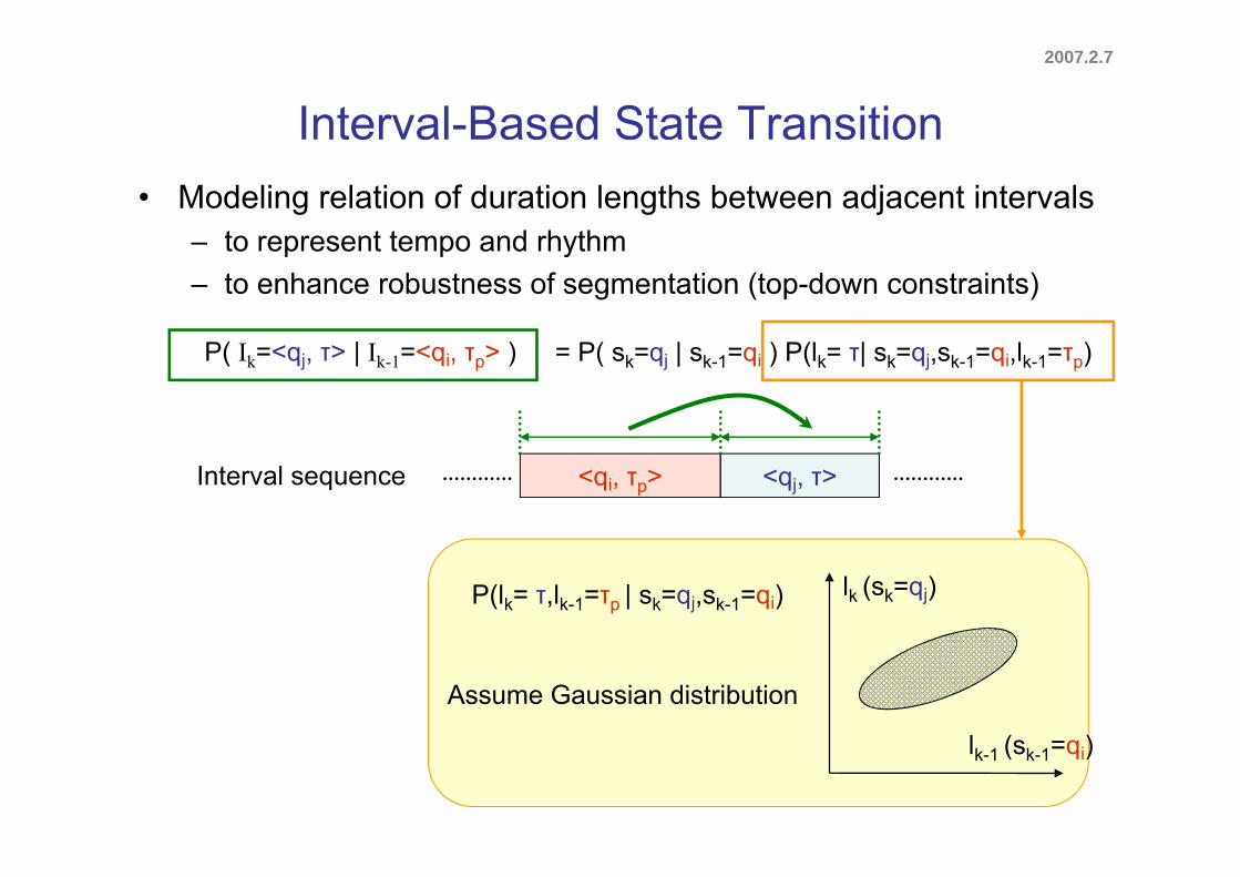
Interval-Based State Transition• Modeling relation of duration lengths between adjacent intervals
to represent tempo and rhythm– to represent tempo and rhythm– to enhance robustness of segmentation (top-down constraints)
P( Ik=<qj, τ> | Ik-1=<qi, τp> ) = P( sk=qj | sk-1=qi ) P(lk= τ| sk=qj,sk-1=qi,lk-1=τp)
<qi, τp> <qj, τ>Interval sequence
P(lk= τ,lk-1=τp | sk=qj,sk-1=qi) lk (sk=qj)
l ( )
Assume Gaussian distribution
lk-1 (sk-1=qi)
2007.2.7
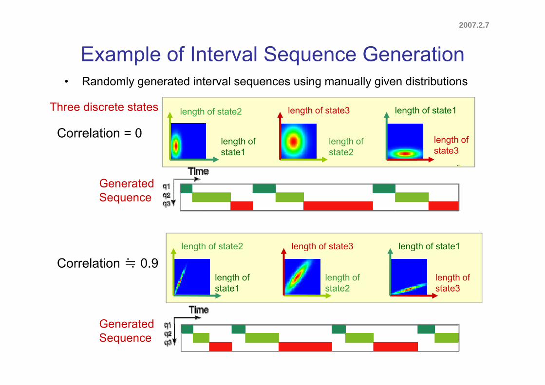
Example of Interval Sequence Generationp q• Randomly generated interval sequences using manually given distributions
Three discrete states
Correlation = 0length oft t 1
length of state2
length oft t 2
length of state3
length ofstate3
length of state1Three discrete states
state1 state2 state3
GeneratedSequence
Correlation ≒ 0.9length of
length of state2
length of
length of state3
length of
length of state1
length ofstate1
length ofstate2
length ofstate3
GeneratedGeneratedSequence
2006.11.21
Chapter 3
Learning Method for the Interval-Based Hybrid Dynamical System
2007.2.7
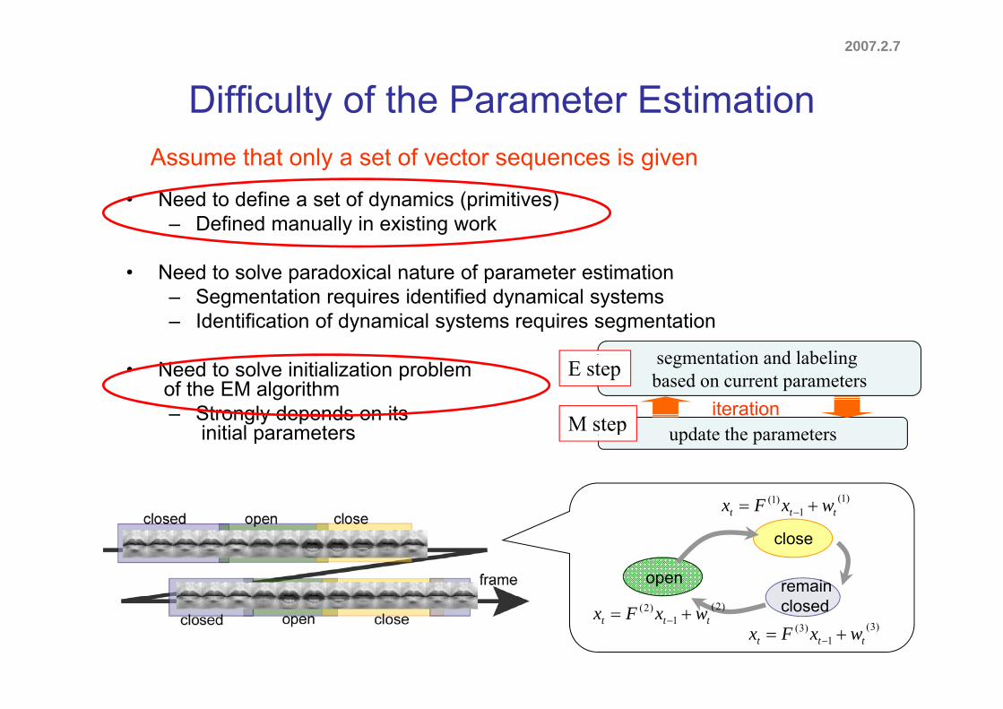
Difficulty of the Parameter Estimationy
N d t d fi t f d i ( i iti )
Assume that only a set of vector sequences is given
• Need to define a set of dynamics (primitives)– Defined manually in existing work
• Need to solve paradoxical nature of parameter estimation• Need to solve paradoxical nature of parameter estimation– Segmentation requires identified dynamical systems – Identification of dynamical systems requires segmentation
t ti d l b li• Need to solve initialization problemof the EM algorithm – Strongly depends on its
initial parameters
segmentation and labeling based on current parameters
update the parameters
E step
M stepiteration
initial parameters update the parametersp
)1(1
)1(ttt wxFx
remainopen
close
1 ttt
closed)2(1
)2(ttt wxFx )3(
1)3(
ttt wxFx
2007.2.7
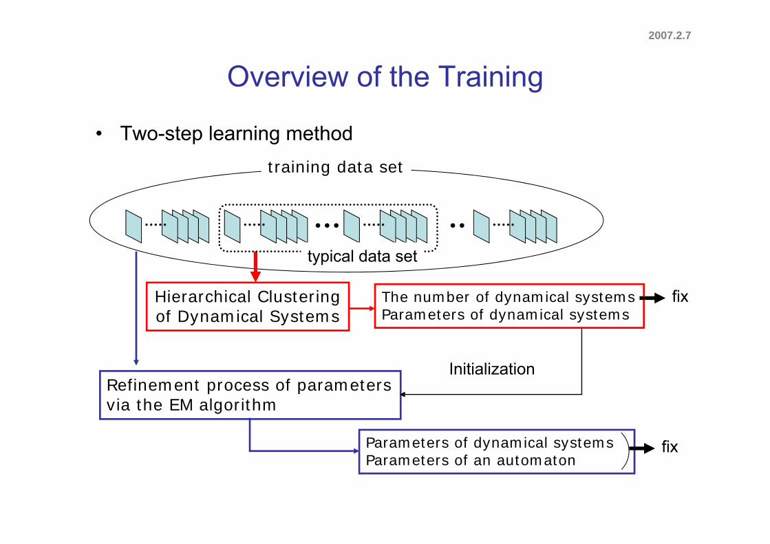
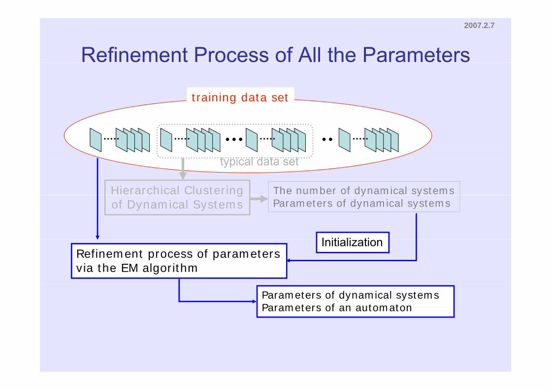
Overview of the Trainingg
• Two-step learning methodtraining data set
typical data set
The number of dynamical systemsParameters of dynamical systems
Hierarchical Clustering of Dynamical Systems
fix
Refinement process of parametersInitialization
Parameters of dynamical systemsParameters of an automaton
via the EM algorithm
fixParameters of an automaton
2007.2.7
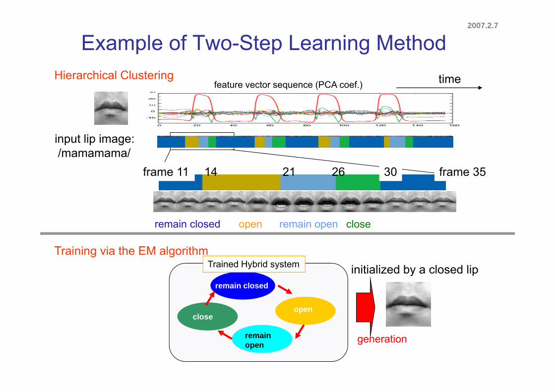
Example of Two-Step Learning MethodtimeHierarchical Clustering
feature vector sequence (PCA coef.)
input lip image:/mamamama//mamamama/
frame 11 frame 3514 21 26 30
remain closed open remain open close
remain closed
Trained Hybrid system initialized by a closed lipTraining via the EM algorithm
remain closed
openclose
remainopen generation
2007.2.7
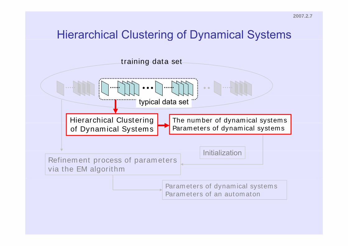
Hierarchical Clustering of Dynamical Systems
training data set
g y y
typical data set
The number of dynamical systemsHierarchical Clustering y yParameters of dynamical systems
I iti li ti
gof Dynamical Systems
Refinement process of parametersvia the EM algorithm
Initialization
Parameters of dynamical systemsParameters of an automaton
2007.2.7
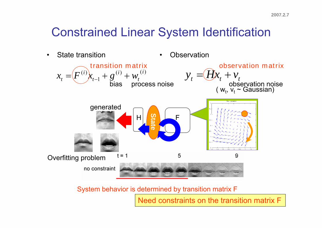
Constrained Linear System Identification
• State transition • Observation
y
)()(1
)( it
it
it wgxFx ttt vHxy
transition matrix observation matrix
bias process noise observation noise( w v Gaussian)
Sgenerated
( wt, vt ~ Gaussian)
FH
StateOverfitting problem
System behavior is determined by transition matrix F
Need constraints on the transition matrix Fy y
2007.2.7
Class of Linear Dynamical Systemsy y
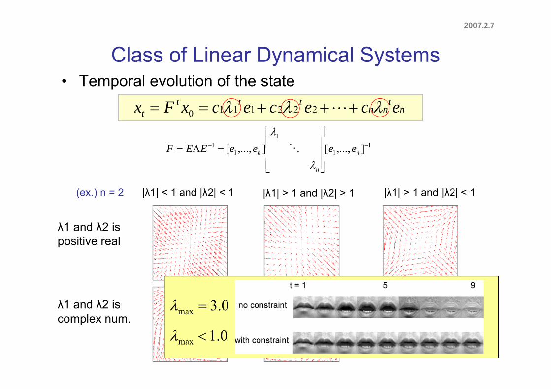
tttt ecececxFx 222111
• Temporal evolution of the state
nnnt ecececxFx 2221110
11
1 ][][
eeeeEEF
|λ1| > 1 and |λ2| > 1|λ1| < 1 and |λ2| < 1 |λ1| > 1 and |λ2| < 1
11 ],...,[],...,[
n
n
n eeeeEEF
(ex ) n = 2 |λ1| > 1 and |λ2| > 1|λ1| < 1 and |λ2| < 1 |λ1| > 1 and |λ2| < 1
λ1 and λ2 is iti l
(ex.) n 2
positive real
λ1 and λ2 iscomplex num. NA0.3max
0.1max
2007.2.7
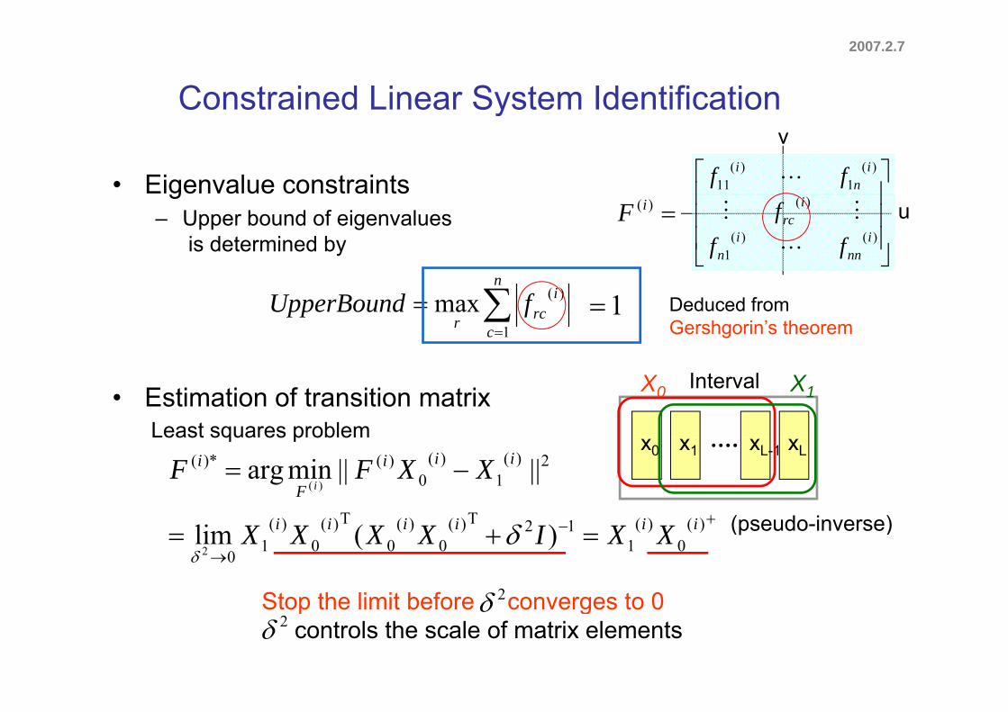
Constrained Linear System Identificationy
• Eigenvalue constraints
v
)(
1)(
11i
ni ff g
– Upper bound of eigenvaluesis determined by
u
)()(
1
)(
inn
in
irc
fff
)(iF
n
c
ircr
fUpperBound1
)(max Deduced fromGershgorin’s theorem
1
• Estimation of transition matrix X0 X1
Least squares problem
Interval
TT
2)(1
)(0
)()*( ||||minarg)(
iii
F
i XXFFi
x0 x1 xLxL-1
( d i )
Least squares problem
)(
0)(
112T)(
0)(
0
T)(0
)(1
0)(lim
2
iiiiii XXIXXXX
2Stop the limit before converges to 0
(pseudo-inverse)
22
Stop the limit before converges to 0controls the scale of matrix elements
2007.2.7
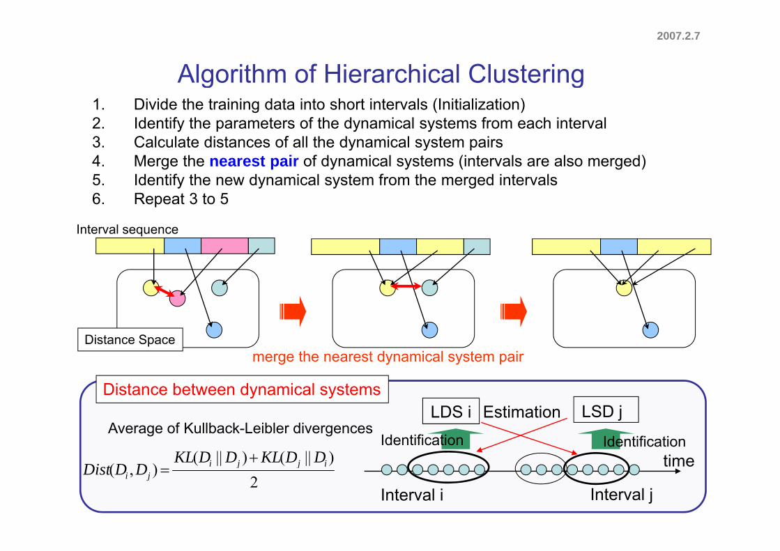
Algorithm of Hierarchical Clusteringg g1. Divide the training data into short intervals (Initialization)2. Identify the parameters of the dynamical systems from each interval3. Calculate distances of all the dynamical system pairsy y p4. Merge the nearest pair of dynamical systems (intervals are also merged)5. Identify the new dynamical system from the merged intervals6. Repeat 3 to 5
Interval sequence
Distance Spacemerge the nearest dynamical system pair
Distance Space
Distance between dynamical systems
time
LDS i LSD j
Identification Identification
EstimationAverage of Kullback-Leibler divergences
)||()||( ijji DDKLDDKL time
Interval i Interval j2
)||()||(),( ijji
ji DDDist
2007.2.7
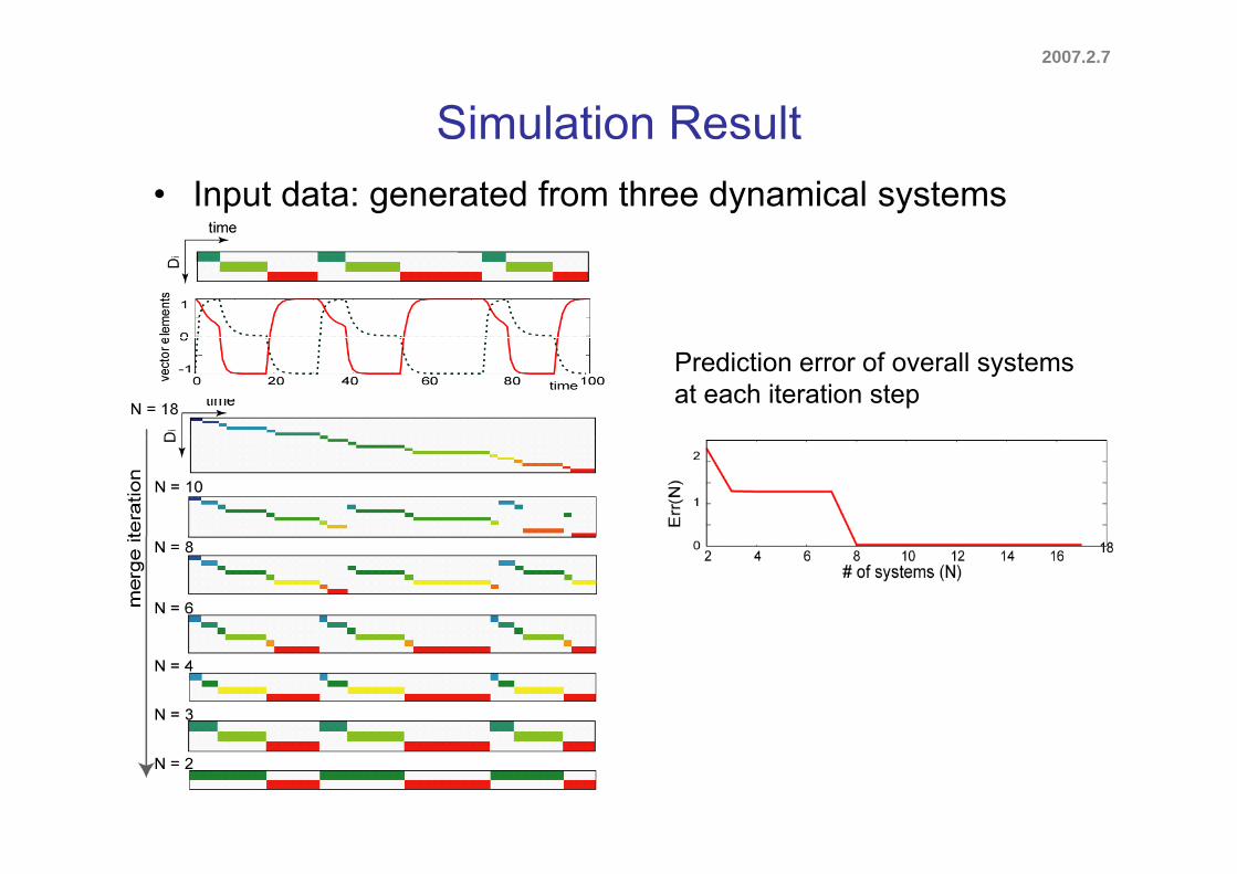
Simulation Result• Input data: generated from three dynamical systems
Prediction error of overall systems at each iteration step
2007.2.7
Refinement Process of All the Parameters
training data set
The number of dynamical systemsHierarchical Clustering
typical data set
y yParameters of dynamical systems
I iti li ti
gof Dynamical Systems
Refinement process of parametersvia the EM algorithm
Initialization
Parameters of dynamical systemsParameters of an automaton
2007.2.7
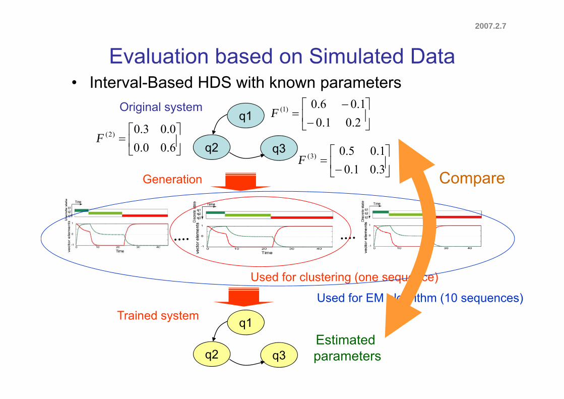
Evaluation based on Simulated Data• Interval-Based HDS with known parameters
1.06.0)1(FOriginal system
q2
q1
q3
2.01.0
)1(F
1.05.0)3(
6.00.00.03.0)2(F
Original system
q
3.01.01.05.0)3(F
CompareGeneration
Used for clustering (one sequence)
Used for EM algorithm (10 sequences)
q1Trained system
E ti t dq2 q3
Estimatedparameters
2007.2.7
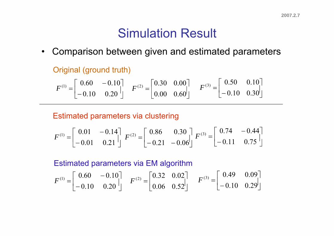
Simulation Result• Comparison between given and estimated parameters
10.060.0)1(F
30010010.050.0)3(F
00.030.0)2(F
Original (ground truth)
20.010.0
30.010.0
60.000.0
Estimated parameters via clustering
21.001.014.001.0)1(F
75.011.044.074.0)3(F
06.021.0
30.086.0)2(F
Estimated parameters via clustering
21.001.0 06.021.0
Estimated parameters via EM algorithm
20.010.010.060.0)1(F
29.010.009.049.0)3(F
52.006.002.032.0)2(F
2007.2.7
Discussion
• Interval-based hybrid dynamical systemInterval based state transition to model tempo and rhythm– Interval-based state transition to model tempo and rhythm
– Linear dynamics to model continuously changing patterns
• Two-step learning method for the interval-based– Clustering of dynamical systems + EM algorithm
Constrained system identification based on eigenvalues– Constrained system identification based on eigenvalues
2006.11.21
Chapter 4
Analysis of Timing Structures in Multipart Motion of Facial Expression
2007.2.7
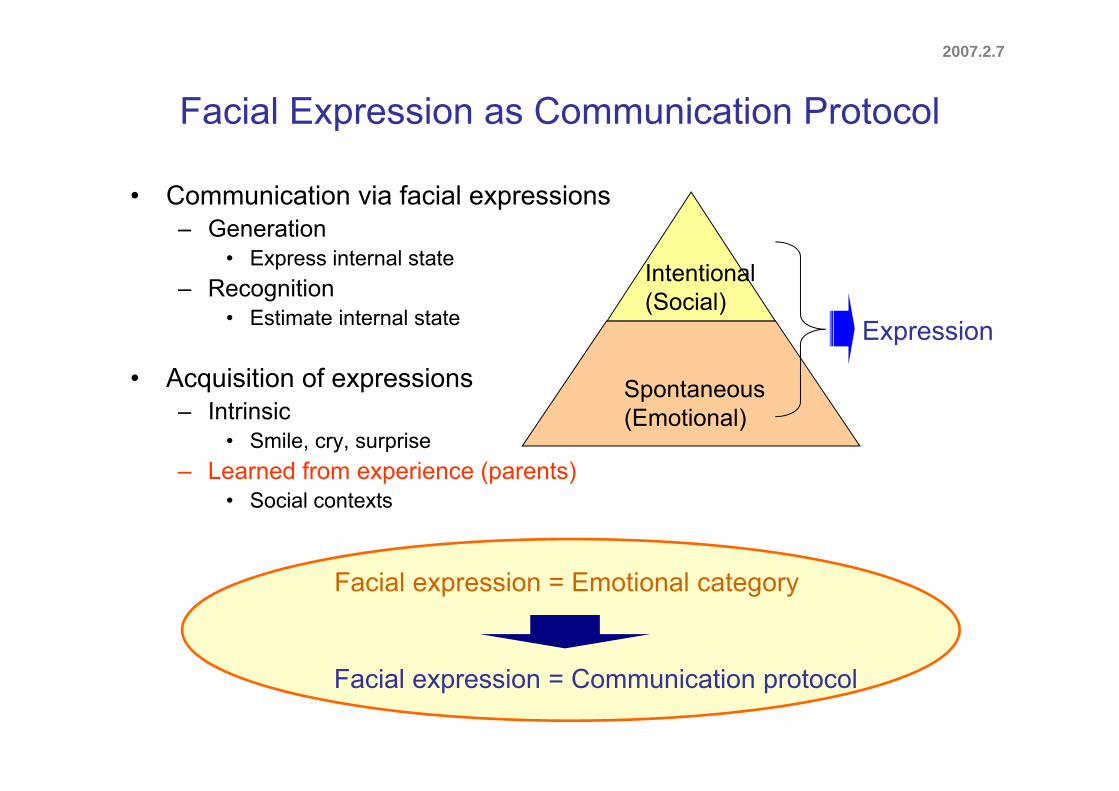
Facial Expression as Communication Protocolp
• Communication via facial expressions– Generation
• Express internal state– Recognition Intentional
(Social)• Estimate internal state
• Acquisition of expressions
Expression
Spontaneous
(Social)
– Intrinsic• Smile, cry, surprise
– Learned from experience (parents)
Spontaneous(Emotional)
• Social contexts
F i l i E ti l tFacial expression = Emotional category
Facial expression = Communication protocol
2007.2.7
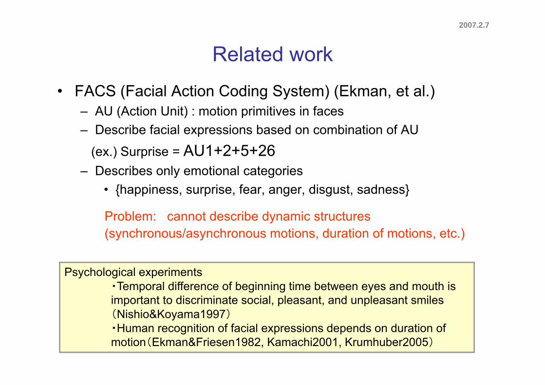
Related work
• FACS (Facial Action Coding System) (Ekman, et al.)– AU (Action Unit) : motion primitives in faces– Describe facial expressions based on combination of AU
( ) S i AU1+2+5+26(ex.) Surprise = AU1+2+5+26– Describes only emotional categories
• {happiness, surprise, fear, anger, disgust, sadness}{happiness, surprise, fear, anger, disgust, sadness}
Problem: cannot describe dynamic structures (synchronous/asynchronous motions duration of motions etc )
Psychological experiments
(synchronous/asynchronous motions, duration of motions, etc.)
・Temporal difference of beginning time between eyes and mouth is important to discriminate social, pleasant, and unpleasant smiles(Nishio&Koyama1997)
f f f・Human recognition of facial expressions depends on duration of motion(Ekman&Friesen1982, Kamachi2001, Krumhuber2005)
2007.2.7
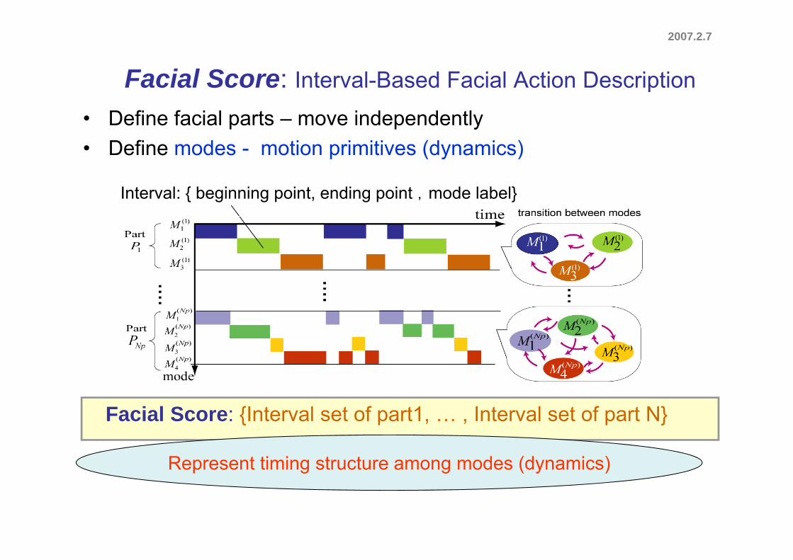
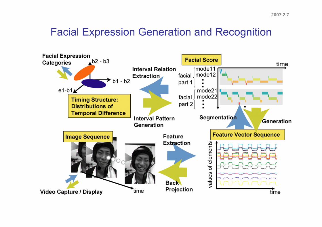
Facial Score: Interval-Based Facial Action Descriptionp
• Define facial parts – move independently• Define modes - motion primitives (dynamics)Define modes motion primitives (dynamics)
Interval: { beginning point, ending point ,mode label}
F i l S {I t l t f t1 I t l t f t N}Facial Score: {Interval set of part1, … , Interval set of part N}
Represent timing structure among modes (dynamics)p g g ( y )
2007.2.7
Facial Expression Generation and Recognitionp g
2007.2.7
1 Definition of Facial Scores1. Definition of Facial Scores2. Automatic Acquisition of Facial Scores3 Evaluation3. Evaluation
Definition of partsDefinition of partsDefinition of modes
2007.2.7
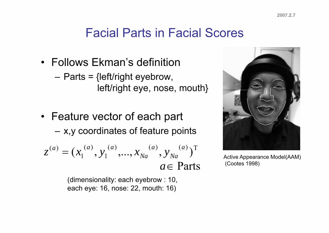
Facial Parts in Facial Scores
• Follows Ekman’s definitionFollows Ekman s definition– Parts = {left/right eyebrow,
left/right eye nose mouth}left/right eye, nose, mouth}
• Feature vector of each part• Feature vector of each part– x,y coordinates of feature points
Τ)()()(1
)(1
)( ),,...,,( aNa
aNa
aaa yxyxz Active Appearance Model(AAM)(Cootes 1998)Partsa
(dimensionality: each eyebrow : 10, each eye: 16, nose: 22, mouth: 16)
Partsa
2007.2.7
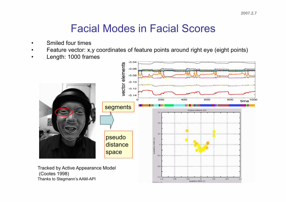
Facial Modes in Facial Scores• Smiled four times• Feature vector: x,y coordinates of feature points around right eye (eight points)
L th 1000 f• Length: 1000 frames
segments
pseudodistance
Tracked by Active Appearance Model
space
y pp(Cootes 1998)
Thanks to Stegmann’s AAM-API
2007.2.7
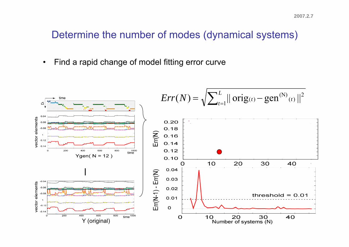
Determine the number of modes (dynamical systems)( y y )
• Find a rapid change of model fitting error curve
LNE 2(N) ||i||)(
tttNErr
12
)((N)
)( ||genorig||)(
Y (original)
2007.2.7
1 Definition of Facial Scores1. Definition of Facial Scores2. Automatic Acquisition of Facial Scores3 Evaluation3. Evaluation
Generation of expressions Generation of expressions Discrimination of expressions
2007.2.7
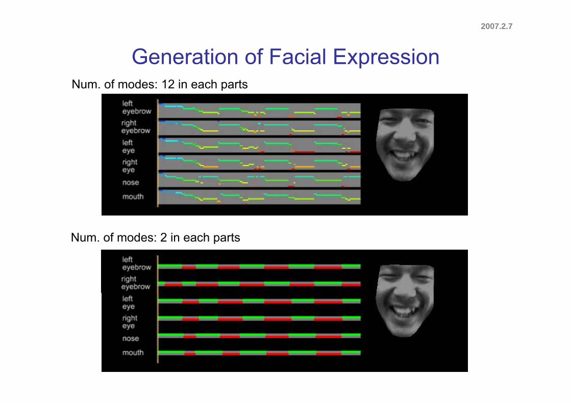
Generation of Facial ExpressionpNum. of modes: 12 in each parts
Num. of modes: 2 in each parts
2007.2.7
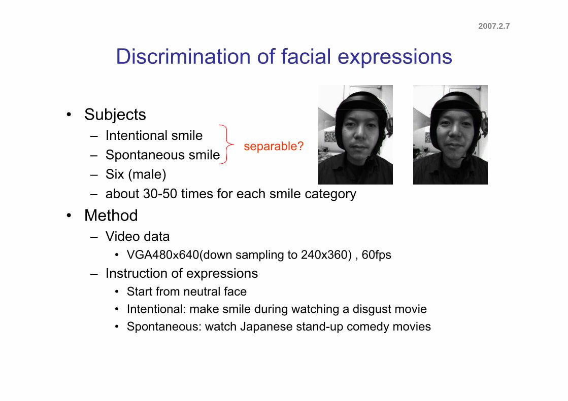
Discrimination of facial expressionsp
S bj t• Subjects– Intentional smile
Spontaneous smileseparable?
– Spontaneous smile– Six (male)– about 30-50 times for each smile categoryg y
• Method– Video data
• VGA480x640(down sampling to 240x360) , 60fps– Instruction of expressions
• Start from neutral face• Start from neutral face• Intentional: make smile during watching a disgust movie• Spontaneous: watch Japanese stand-up comedy movies
2007.2.7
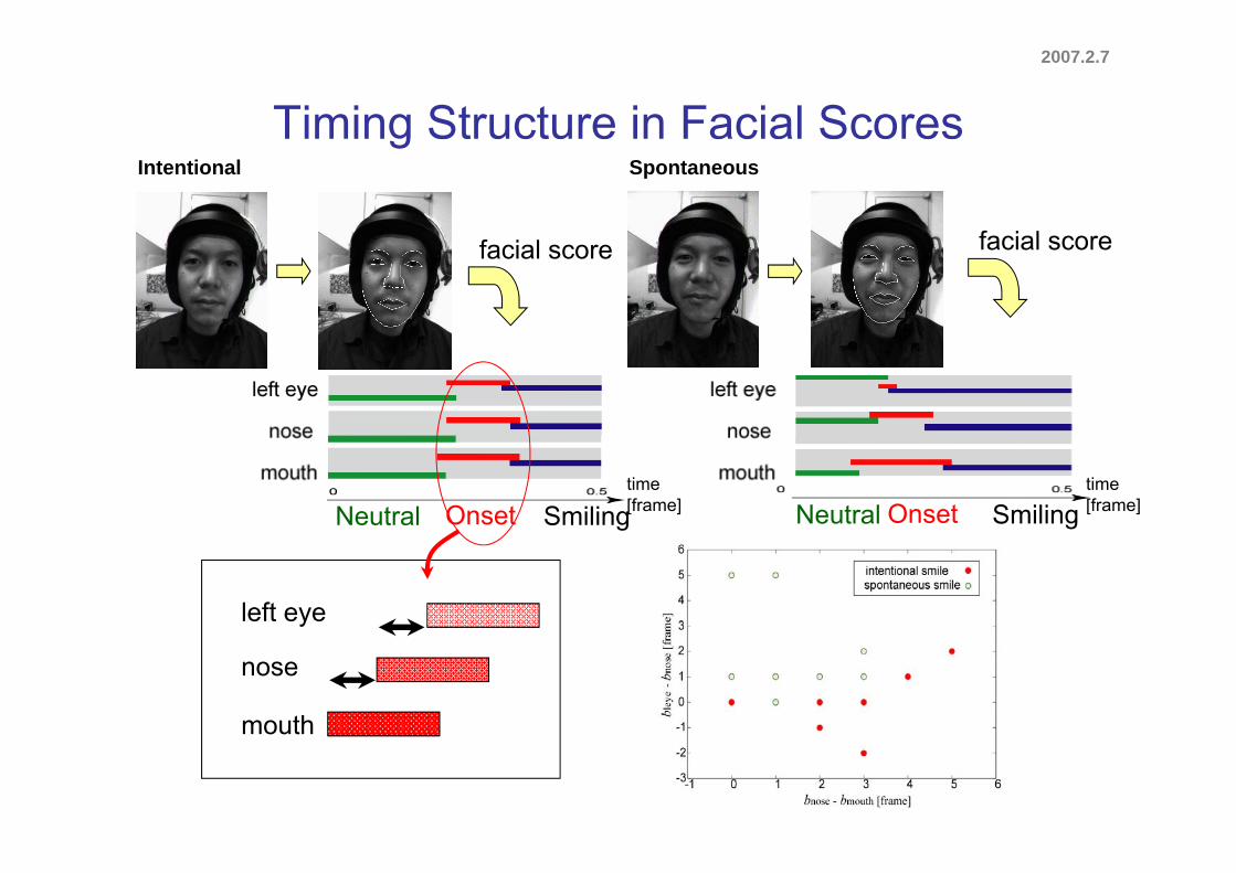
Timing Structure in Facial ScoresIntentional Spontaneous
facial score
g
facial score facial score
Neutral Onset Smiling Neutral Onset Smilingtime[frame]
time[frame]
left eye
nose
mouthmouth
2007.2.7
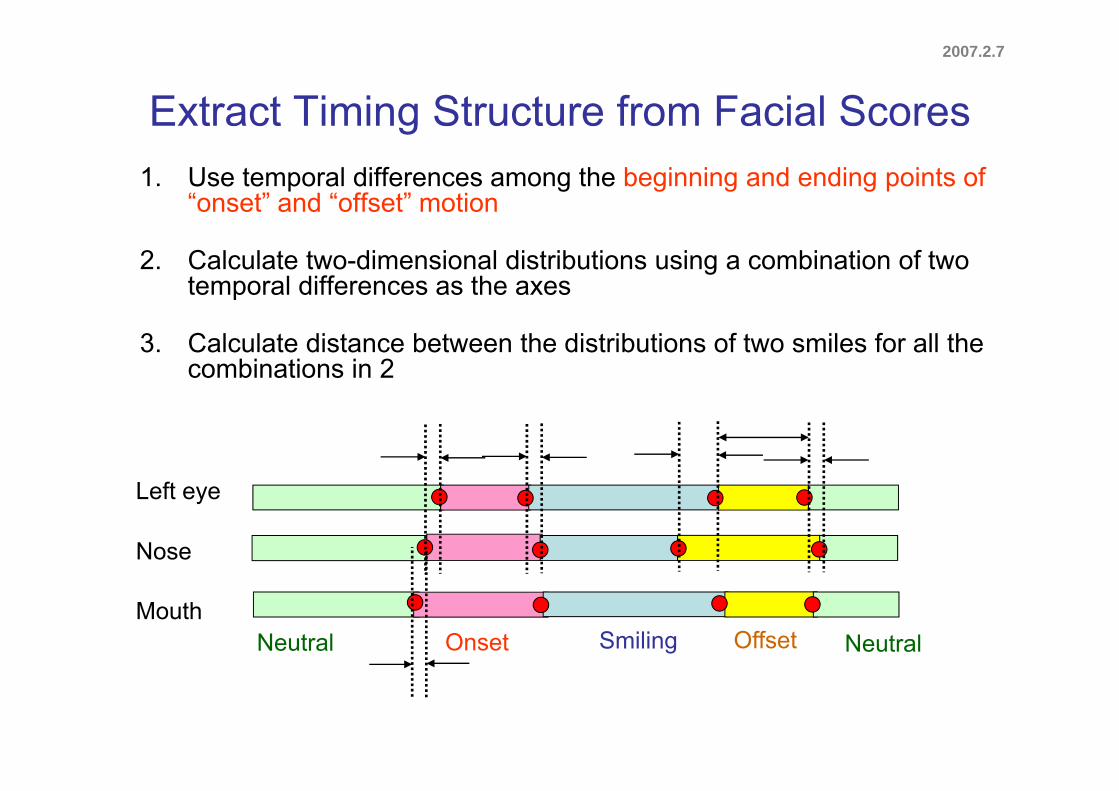
Extract Timing Structure from Facial Scoresg1. Use temporal differences among the beginning and ending points of
“onset” and “offset” motion
2. Calculate two-dimensional distributions using a combination of two temporal differences as the axes
3. Calculate distance between the distributions of two smiles for all the combinations in 2
L ftLeft eye
Nose
Neutral NeutralSmilingOnset OffsetMouth
2007.2.7
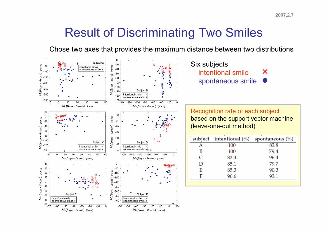
Result of Discriminating Two SmilesgChose two axes that provides the maximum distance between two distributions
Six subjectsSix subjectsintentional smilespontaneous smile
Recognition rate of each subjectbased on the support vector machine(leave-one-out method)
2007.2.7
Discussion• Analysis of timing structure in multipart motion of
facial expressionfacial expression– Successfully discriminated and recognized intentional and
spontaneous smiles
1 L t b ti ( id t i )Future Work
1. Long term observation (video capturing) Find expression categories in a bottom-up manner
2 Expression in a context2. Expression in a context conversation, singing, watching movies relation among multiple subjects relation among multiple subjects
3. Personality Common structure and modes Specific structure and modes
2006.11.21
Chapter 5
Modeling Timing Structures in Multimedia Signalsg g g
2007.2.7
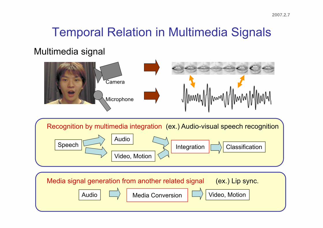
Temporal Relation in Multimedia Signalsp gMultimedia signal
Camera
Microphone
Recognition by multimedia integration (ex.) Audio-visual speech recognition
AudioClassificationSpeech Integration
Audio
Video, Motion
Media signal generation from another related signal (ex.) Lip sync.
Audio Video, MotionMedia Conversion
2007.2.7
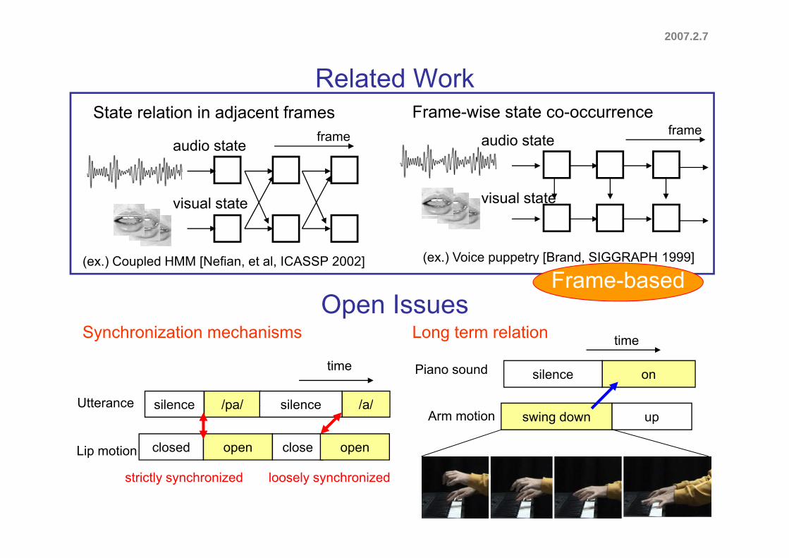
Related WorkState relation in adjacent frames
frame
Frame-wise state co-occurrence frame
audio state audio state
visual state visual state
(ex.) Coupled HMM [Nefian, et al, ICASSP 2002] (ex.) Voice puppetry [Brand, SIGGRAPH 1999]
Frame based
time
Open IssuesSynchronization mechanisms Long term relation
Frame-based
onsilencePiano sound
time
/pa/silence silence /a/Utterance
time
swing down upArm motion/pa/silence silence /a/Utterance
closed open close openLip motion
strictly synchronized loosely synchronized
2007.2.7
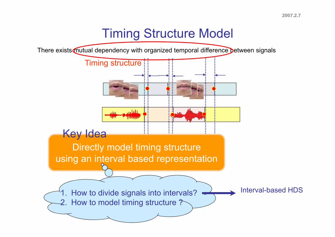
Timing Structure ModelgThere exists mutual dependency with organized temporal difference between signals
Timing structureTiming structure
Directly model timing structureKey Idea
Directly model timing structureusing an interval based representation
1. How to divide signals into intervals? Interval-based HDS
2. How to model timing structure ?
2007.2.7
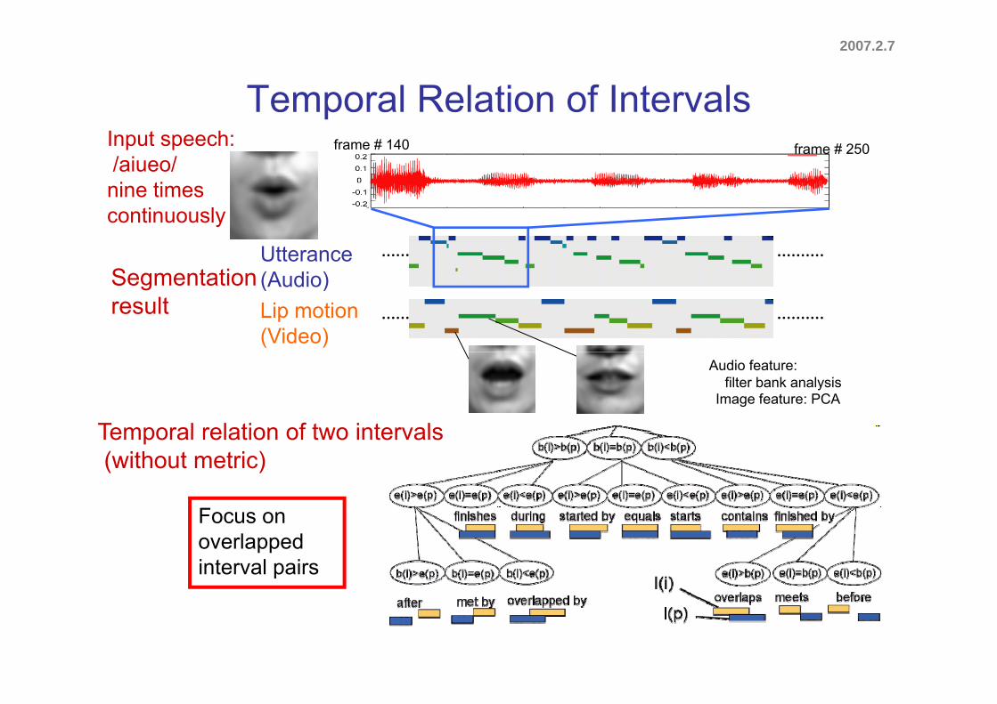
Temporal Relation of Intervalspframe # 140 frame # 250Input speech:
/aiueo/nine times
Utterance(A di )S t ti
nine timescontinuously
(Audio)Lip motion(Video)
Segmentationresult
Temporal relation of two intervalsImage feature: PCA
Audio feature:filter bank analysis
Foc s on
Temporal relation of two intervals(without metric)
Focus on overlappedinterval pairs
2007.2.7
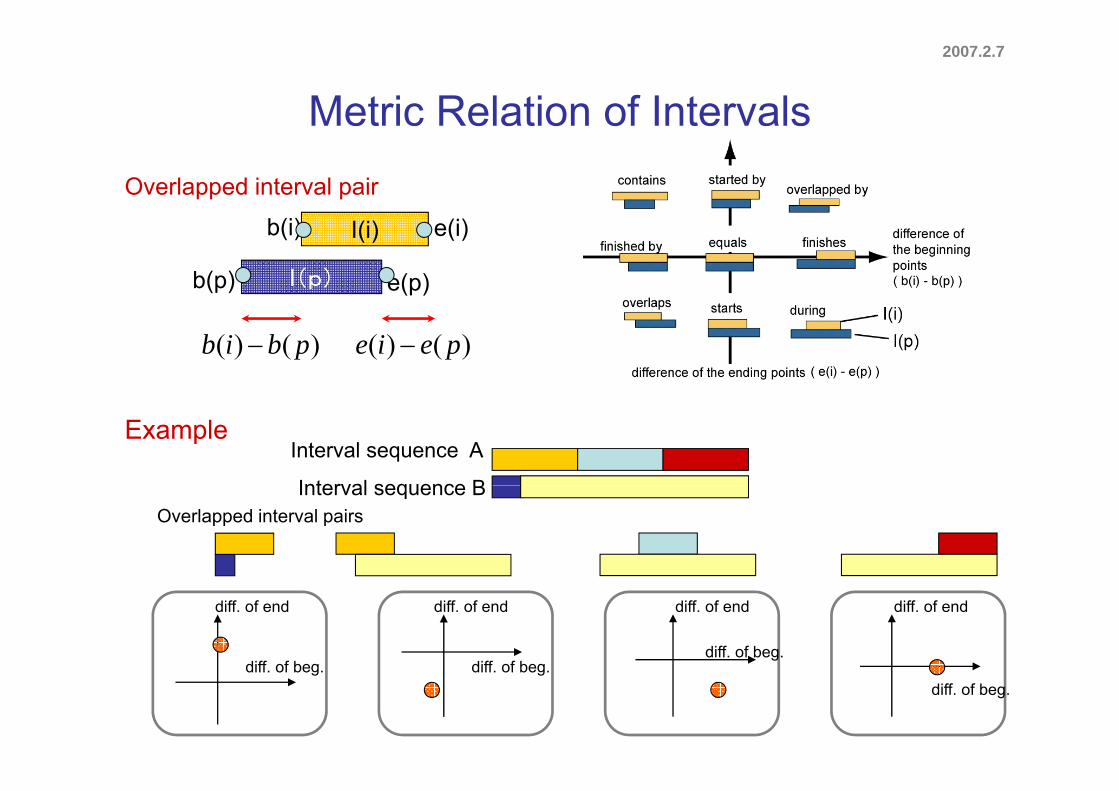
Metric Relation of IntervalsOverlapped interval pair
I(i)
I(p)
b(i) e(i)
b(p) e(p)
)()( pbib )()( peie
Interval sequence A
Interval sequence B
Example
Overlapped interval pairsInterval sequence B
diff of beg diff of begdiff. of beg.
diff. of end diff. of end diff. of end diff. of end
diff. of beg. diff. of beg.diff. of beg.
2007.2.7
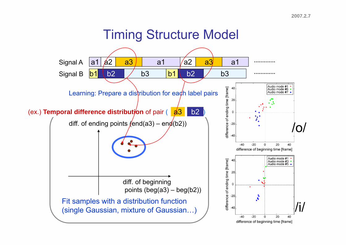
Timing Structure Modelg
a2 a3 a1Signal A a2 a3 a1a1b1 b2Signal B b3 b1 b2 b3
Learning: Prepare a distribution for each label pairs
diff of ending points (end(a3) end(b2))
Learning: Prepare a distribution for each label pairs
(ex.) Temporal difference distribution of pair ( )a3 b2
/ /diff. of ending points (end(a3) – end(b2)) /o/
Fit samples with a distribution function
diff. of beginningpoints (beg(a3) – beg(b2))
/i/(single Gaussian, mixture of Gaussian…) /i/
2007.2.7
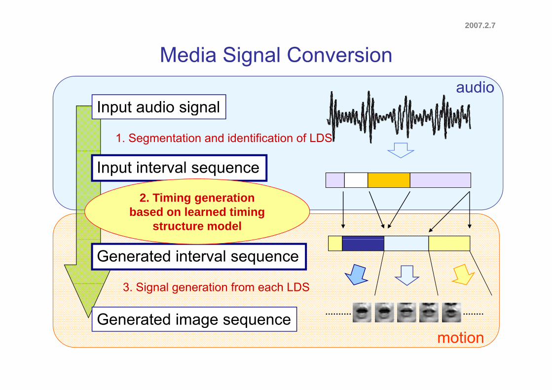
Media Signal Conversiong
Input audio signalaudio
Input audio signal
1. Segmentation and identification of LDS
Input interval sequence
2 Ti i ti2. Timing generation based on learned timing
structure model
Generated interval sequence
3 Si l ti f h LDS
Generated image sequence
3. Signal generation from each LDS
gmotion
2007.2.7
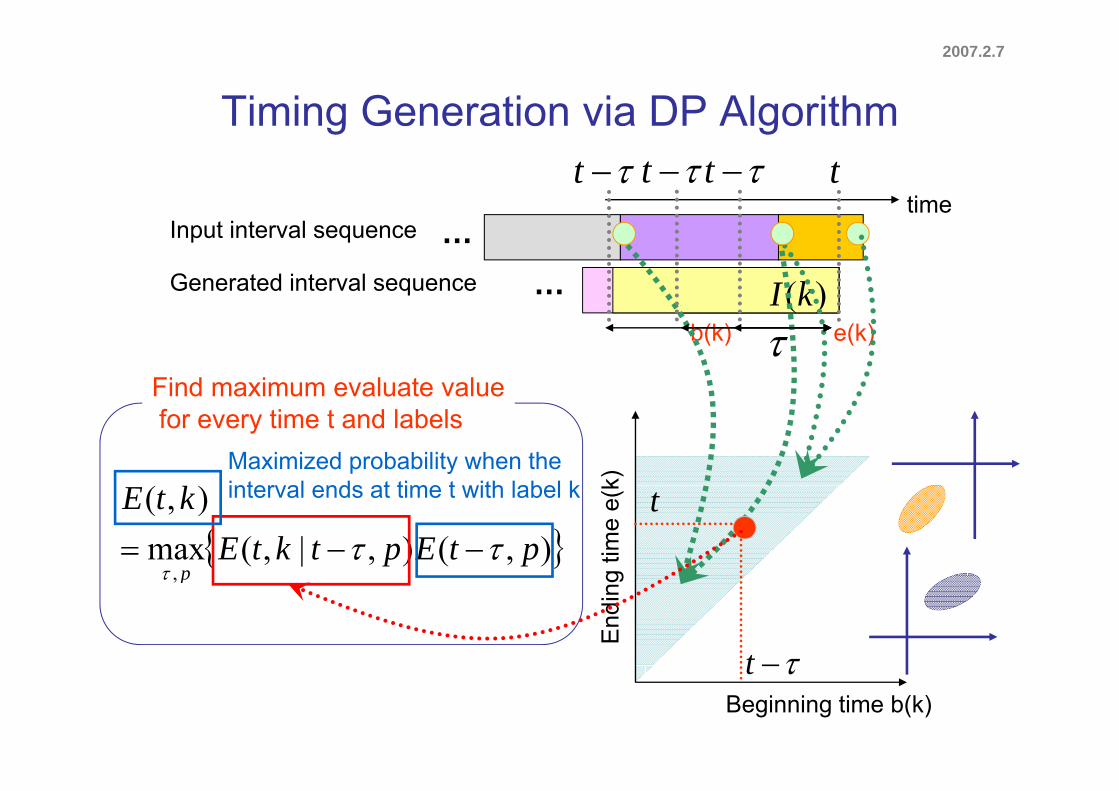
Timing Generation via DP Algorithmg gt
timettt
Input interval sequence
Generated interval sequence
…… )(kI
b(k) e(k)
Find maximum evaluate value
)(k
k)
Find maximum evaluate valuefor every time t and labels
Maximized probability when theinterval ends at time t with label k
g tim
e e(
k
),(),|,(max),(
ptEptktEktE
p
interval ends at time t with label k t
End
ing, p
tBeginning time b(k)
t
2007.2.7
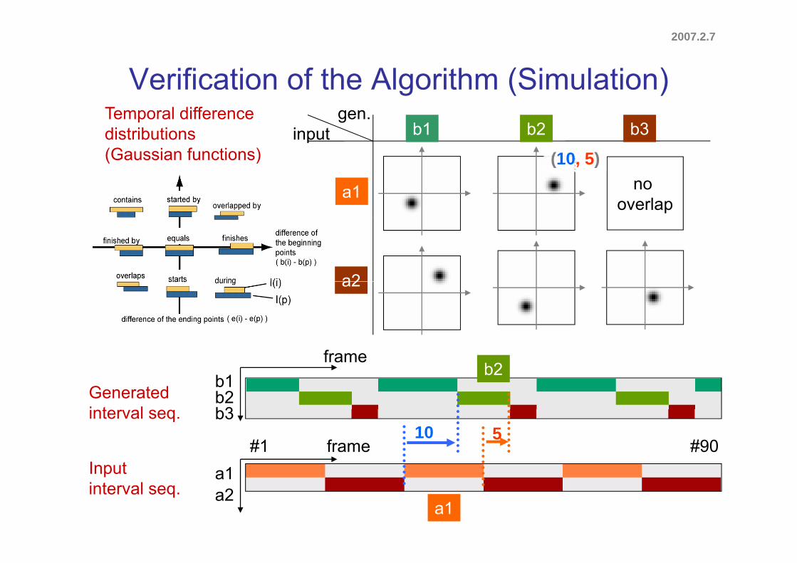
Verification of the Algorithm (Simulation)g ( )Temporal difference distributions (Gaussian functions)
b1 b2 b3inputgen.
(10 5)(Gaussian functions)
no overlap
a1
(10, 5)
a2a2
Generatedi t l
b1b2
frame
b3
b2
Input
interval seq.
a1frame
b310 5
#90#1Inputinterval seq.
a1a2
a1
2007.2.7
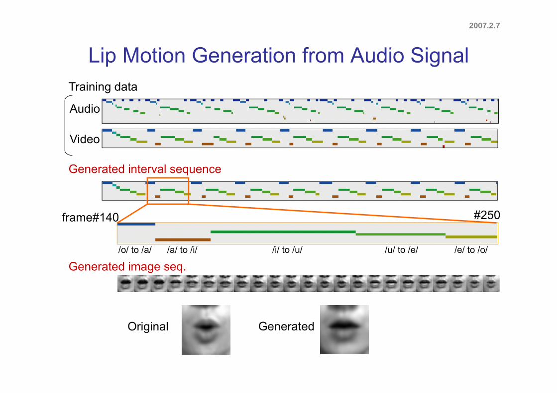
Lip Motion Generation from Audio Signalp gTraining data
AudioAudio
Video
Generated interval sequence
#250frame#140
Generated image seq./i/ to /u/ /u/ to /e/ /e/ to /o//a/ to /i//o/ to /a/
GeneratedOriginal Ge e atedOriginal
2007.2.7
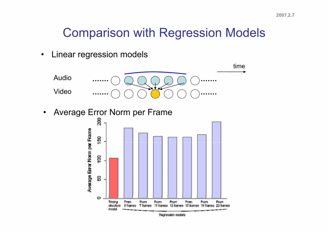
Comparison with Regression Modelsp g• Linear regression models
time
Audio
Vid
• Average Error Norm per Frame
Video
g p
2007.2.7
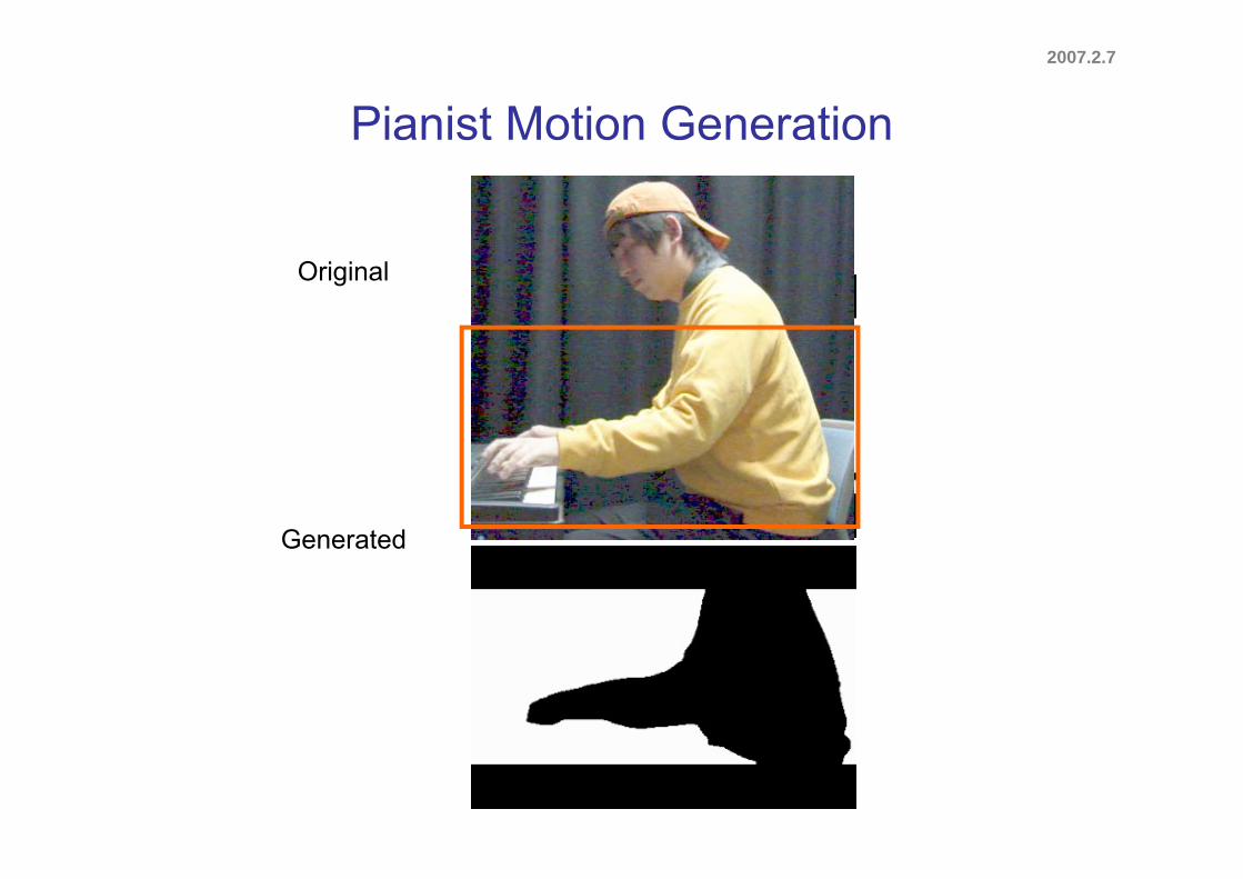
Pianist Motion Generation
Original
GeneratedGenerated
2007.2.7
Discussion
• Timing structure model– Explicitly represents temporal metric relation between media signals
• Media conversion based on the timing structure model– Generates timing of one signal from other related media signals
• Apply to human-computer interaction
Future workApply to human computer interaction(ex.)– audio-visual speech recognitiong– facial expression analysis– speaker detection in noisy environment– utterance timing generation for speech dialog system
2006.11.21
Chapter 6
ConclusionConclusion
2007.2.7
Summaryy
• Interval-based hybrid dynamical systemsi t t di t t t ( bj ti ti ) d– integrate discrete-event systems (subjective time) anddynamical systems (objective (physical) time)
– explicitly model temporal relations such ast d h th i i l• tempo and rhythm in a signal
• timing structure among different media signalsbased on temporal intervals
• Two-step learning method– Clustering of dynamical systems based on eigenvalue constraintsClustering of dynamical systems based on eigenvalue constraints– Refinement of parameters via the EM algorithm
2007.2.7
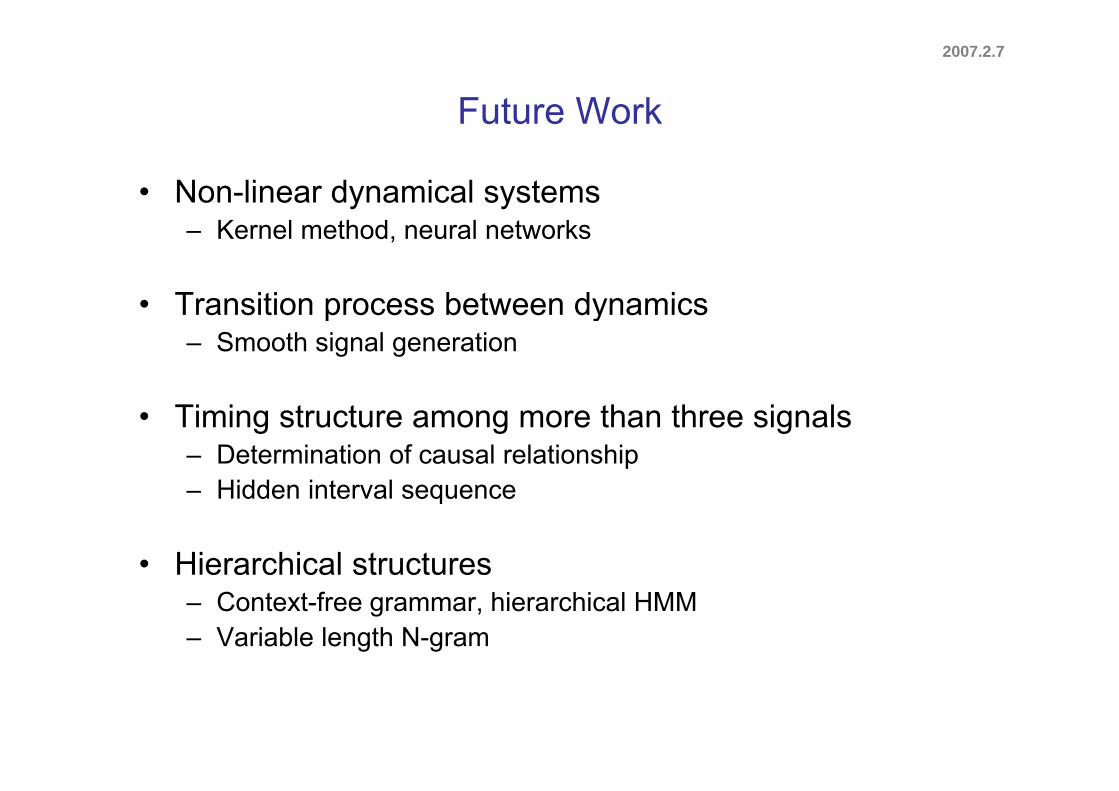
Future Work
• Non-linear dynamical systems– Kernel method, neural networks
• Transition process between dynamics• Transition process between dynamics– Smooth signal generation
• Timing structure among more than three signals– Determination of causal relationship
Hidden interval sequence– Hidden interval sequence
• Hierarchical structures– Context-free grammar, hierarchical HMM– Variable length N-gram
2007.2.7
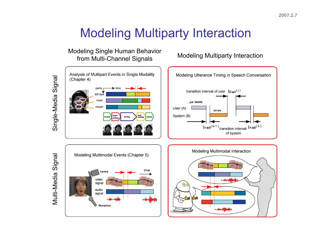
Modeling Multiparty Interactiong p yModeling Single Human Behavior
from Multi-Channel Signals Modeling Multiparty InteractionS
igna
le-
Med
ia S
Sin
glS
igna
lul
ti-M
edia
SM
u


![Logics of Dynamical Systems - cs.cmu.eduaplatzer/pub/lds-lics.pdf · ical systems described by differential equations [44], and hybrid dynamical systems alias hybrid systems combining](https://img.dokumen.tips/doc/110x75/5f06b1f57e708231d4194613/logics-of-dynamical-systems-cscmu-aplatzerpublds-licspdf-ical-systems-described.jpg)