Interrelationships among International StockMarket Indices: Europe, Asia and the

Americas.

Adel Sharkasi, Heather J. Ruskin and Martin Crane

School of Computing, Dublin City University, Dublin 9, IRELANDEmail: asharkasi, hruskin and mcrane@computing.dcu.ie

June 28, 2004

Abstract

In this paper, we investigate the price interdependence betweenseven international stock markets, namely Irish, UK, Portuguese, US,Brazilian, Japanese and Hong Kong, using a new testing method,based on the wavelet transform to reconstruct the data series, assuggested by Lee (2002). We find evidence of intra-European (Irish,UK and Portuguese) market co-movements with the US market alsoweakly influencing the Irish market. We also find co-movement be-tween the US and Brazilian markets and similar intra-Asian co-movements(Japanese and Hong Kong). Finally, we conclude that the circle of im-pact is that of the European markets (Irish, UK and Portuguese) onboth American markets (US and Brazilian), with these in turn im-pacting on the Asian markets (Japanese and Hong Kong) which inturn influence the European markets. In summary, we find evidencefor intra-continental relationships and an increase in importance ofinternational spillover effects since the mid 1990’s, while the impor-tance of historical transmissions has decreased since the beginning ofthis century.

keywords: Simple Regression, Volatility and Wavelet Analysis

1 Introduction

The relationships between international stock markets have been investigatedin several articles, especially after “Black Monday” (October 1987). These

1

studies indicated that co-movements among stock markets have increasedthe possibilities for national markets to be influenced by changes in for-eign ones. For example, Eun and Shim (1989) investigated the relationshipsamong nine major stock markets (Australia, Canada, France, Germany, HongKong, Japan, Switzerland, the UK and the US) using the Vector Autoregres-sive (VAR) model and reported that news beginning in the US market hasthe most influence on the other markets. Lin at el (1994) studied the inter-dependence between the returns and volatility of Japan and the US marketindices using daytime and overnight returns. The results indicated that day-time returns in each market (US or Japan) are linked with the overnightreturns in the other.

In addition, Kim and Rogers (1995) used GARCH1 to study the co-movements between the stock markets of Korea, Japan, and the US andtheir result indicated that the spillovers from Japan and the US have in-creased since the Korean market became open for outsiders to own shares.Further, Booths et al. (1997) reported that there are significant spillovereffects among Scandinavian stock markets (Danish, Norwegian, Swedish andFinnish) applying EGARCH2. Additionally, CVM3 (1998) investigated thelink between the Asian and Brazilian markets as representative of the LatinAmerican region during 1997. They found that the spillover effect startedon July 15th with the Thailand currency crisis. However, this spillover wasnot clearly observed until after October 23rd (the Hong Kong crash). In arecent study, Ng (2000) found significant spillover effects from Japan andthe US stock market on six Pacific-Basin markets, namely those of HongKong, Korea, Malaysia, Singapore, Taiwan and Thailand. In order to studyinternational transmission effects of this type, a new testing technique basedon the wavelet transform, was developed by Lee (2002) and applied to threedeveloped markets (US, Germany and Japan) and two emerging markets inthe MENA4 region, namely Egypt and Turkey. The author reported thatmovements from the developed markets affected the developing markets butnot vice versa.

In addition, Bessler and Yang (2003) employed an error correlation modeland Directed Acyclic Graphs (DAG) to investigate the interdependence amongnine mature markets, namely Japan, US, UK, France, Switzerland, HongKong, Germany, Canada and Australia. Their results showed that bothchanges in European and Hong Kong markets influenced the US market,while this was also affected by internal events. Moreover, Brooks and Ne-

1Generalized Autoregressive Conditionally Heteroskedastic, Bollerslev (1986)2Exponential Generalized Autoregressive Conditionally Heteroskedastic, Nelson (1991)3CVM is the Securities and Exchange Commission of Brazil4MENA stands for the Middle East and North Africa

2

gro (2003) studied the relationship between market co-integration and thedegree to which companies operate internationally. They considered threefactors (global, country-specific and industry-specific) and found that theimportance of the international factor has increased since the 1980’s whilethat of the country-specific factor has decreased on all markets.

Strong evidence of international transmission from the US and Japanesemarkets to Korean and Thai markets during the late 1990’s was presentedby Wongswan (2003), while most recently, Antoniou et al (2003) applied aVAR-EGARCH model to study the relationships among three EU marketsnamely Germany, France and the UK and the results showed some evidenceof co-integration among those countries.

Our goal in this article is to study the evidence of global co-movementsamong seven stock markets, three in Europe (namely Irish, UK, and Por-tuguese), two in the Americas (namely US, and Brazil) and two in Asia(namely Japan and Hong Kong). In particular, we are interested in whetherco-movements are direct (clockwise only) or indirect, impacting of nearest-neighbour (continental grouping) and whether there is global absorption ofmajor events or large changes in worldwide markets.

The remainder of this paper is organized as follows: The method due toLee (2002) and based on the wavelet transform is described below (Section2), with data and results presented in Section 3. Conclusions and remarksform the final section.

2 Wavelet Analysis

The wavelet transform was introduced to solve problems associated with theFourier transform, when dealing with non-stationary signals, or when dealingwith signals which are localized in time or space as well as frequency. TheWavelet Transform (WT) has been explained in more detail, particularlyin [Hijmans (1993), Bruce and Gao (1996), Gonghui et al (1999) and Lee(2002)], and we give a brief outline only in the following.

2.1 Definition of Wavelet Transform

The wavelet transform (WT) is a mathematical tool that can be applied tomany applications such as image analysis, and signal processing. In partic-ular, the discrete wavelet transform (DWT) is useful in dividing the dataseries into components of different frequency, so that each component can bestudied separately to investigate the data series in depth. The wavelets have

3

two types, father wavelets φ and mother wavelets ψ where∫φ(t)dt = 1 and

∫ψ(t)dt = 0

The smooth and low-frequency parts of a signal are described by using the fa-ther wavelets, while the detail and high-frequency components are describedby the mother wavelets. The orthogonal wavelet families have four differ-ent types which are typically applied in practical analysis, namely, the haar,daublets, symmlets and coiflets.The following is a brief synopsis of their features:

• The haar has compact support and is symmetric but, unlike the others, isnot continuous.

• The daublets are continuous orthogonal wavelets with compact support.

• The symmlets have compact support and were built to be as nearly sym-metric as possible.

• The coiflets were built to be nearly symmetric.

A two-scale dilation equation used to calculate the wavelets, father φ(t)and mother ψ(t), is defined respectively by

φ(t) =√

2∑k

�kφ(2t− k) (1)

ψ(t) =√

2∑k

h̄kφ(2t− k) (2)

where �k and h̄k are the low-pass and high-pass coefficients given by

�k =1√2

∫φ(t)φ(2t− k)dt (3)

h̄k =1√2

∫ψ(t)φ(2t− k)dt (4)

The orthogonal wavelet series approximation to a signal f(t) is definedby

f(t) =∑k

sJ,kφJ,k(t) +∑k

dJ,kψJ,k(t) + . . .+∑k

d1,kψ1,k(t) (5)

where J is the number of multiresolution levels (or scales) and k ranges from1 to the number of coefficients in the specified components (or crystals). Thecoefficient sJ,k,dJ,k,. . .,d1,k are the wavelet transform coefficients given by

sJ,k =∫φJ,k(t)f(t)dt (6)

dj,k =∫ψj,k(t)f(t)dt (j = 1, 2, . . . , J) (7)

4

Their magnitude gives a measure of the contribution of the correspond-ing wavelet function to the signal. The functions φJ,k(t) and ψj,k(t) [j =1, 2, . . . , J ] are the approximating wavelet functions generated from φ and ψthrough scaling and translation as follows

φJ,k(t) = 2−J2 φ(2−Jt− k) = 2

−J2 φ[(t− 2Jk)/2J ] (8)

ψJ,k(t) = 2−J2 ψ(2−Jt− k) = 2

−J2 ψ[(t− 2Jk)/2J ] j = 1, 2, . . . , J (9)

2.2 The Discrete Wavelet Transform (DWT)

The discrete wavelet transform is used to compute the coefficient of thewavelet series approximation in Equation(5) for a discrete signal f1, . . . , fn

of finite extent. The DWT maps the vector f = (f1, f2, . . . , fn)′ to a vec-tor of n wavelet coefficients w = (w1, w2, . . . , wn)′ which contains both thesmooth coefficient sJ,k and the detail coefficients dj,k [j = 1, 2, . . . , J ]. ThesJ,k describe the underlying smooth behaviour of the signal at coarse scale 2J

while dJ,k describe the coarse scale deviations from the smooth behaviour anddJ−1,k, . . . , d1,k provide progressively finer scale deviations from the smoothbehaviour.

In the case when n divisible by 2J ; there are n/2 observations in d1,k atthe finest scale 21 = 2 and n/4 observations in d2,k at the second finest scale22 = 4. Likewise, there are n/2J observations in each of dJ,k and sJ,k where

n = n/2 + n/4 + . . .+ n/2J−1 + n/2J + n/2J .

3 Data and Results

3.1 Data Description

The data used in the following analysis consists of the daily prices of stockmarket indices for seven markets, [Irish (IRL), UK, Portuguese (P), US,Brazilian (BR), Japanese (JP) and Hong Kong (HK)], during the period fromMay 1993 to September 2003. We considered the indices ISEQ Overall (IRL),FTSE All Share (UK), PSI20 (P), S&P500 (US), Bovespa (BR), Nikkei 225(JP) and Hang Seng (HK) to be representative of these markets.

As each market uses its local currency for presenting the index values,we use the daily returns instead of using the daily prices where the followingformula applies:

Daily Return = Ln(Pt/Pt−1)

where

5

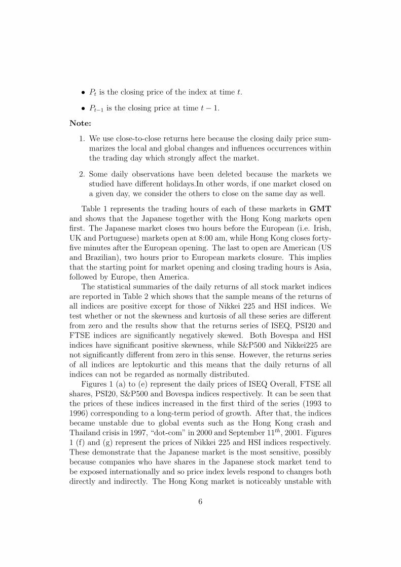
• Pt is the closing price of the index at time t.

• Pt−1 is the closing price at time t− 1.

Note:

1. We use close-to-close returns here because the closing daily price sum-marizes the local and global changes and influences occurrences withinthe trading day which strongly affect the market.

2. Some daily observations have been deleted because the markets westudied have different holidays.In other words, if one market closed ona given day, we consider the others to close on the same day as well.

Table 1 represents the trading hours of each of these markets in GMTand shows that the Japanese together with the Hong Kong markets openfirst. The Japanese market closes two hours before the European (i.e. Irish,UK and Portuguese) markets open at 8:00 am, while Hong Kong closes forty-five minutes after the European opening. The last to open are American (USand Brazilian), two hours prior to European markets closure. This impliesthat the starting point for market opening and closing trading hours is Asia,followed by Europe, then America.

The statistical summaries of the daily returns of all stock market indicesare reported in Table 2 which shows that the sample means of the returns ofall indices are positive except for those of Nikkei 225 and HSI indices. Wetest whether or not the skewness and kurtosis of all these series are differentfrom zero and the results show that the returns series of ISEQ, PSI20 andFTSE indices are significantly negatively skewed. Both Bovespa and HSIindices have significant positive skewness, while S&P500 and Nikkei225 arenot significantly different from zero in this sense. However, the returns seriesof all indices are leptokurtic and this means that the daily returns of allindices can not be regarded as normally distributed.

Figures 1 (a) to (e) represent the daily prices of ISEQ Overall, FTSE allshares, PSI20, S&P500 and Bovespa indices respectively. It can be seen thatthe prices of these indices increased in the first third of the series (1993 to1996) corresponding to a long-term period of growth. After that, the indicesbecame unstable due to global events such as the Hong Kong crash andThailand crisis in 1997, “dot-com” in 2000 and September 11th, 2001. Figures1 (f) and (g) represent the prices of Nikkei 225 and HSI indices respectively.These demonstrate that the Japanese market is the most sensitive, possiblybecause companies who have shares in the Japanese stock market tend tobe exposed internationally and so price index levels respond to changes bothdirectly and indirectly. The Hong Kong market is noticeably unstable with

6

a disproportionately large number of regionwide crashes (possible due toserial crises: Bird Flu, SARS, etc). The Asian financial crisis had strongdirect effects on the Hong Kong market but it affected Japan’s economy onlyweakly because only 40 % of Japan’s exports go to Asia. In addition, Japanwas going through its own ongoing long-term economic difficulties.

From the above, there are clear indications of effects from regionwidemarkets as well as from worldwide markets and this picture is more detailedwhen we look at the results of the wavelet analysis. The energy percentagesdescribed by each wavelet component for the daily returns of seven marketindices are given in Table 3 which shows that the first two high frequencycrystals (d1 & d2) explain more than 65% of the energy of these series, imply-ing that movements are mainly caused by short-term fluctuations. Figures 2(a) to (g) represent the discrete wavelet transform (DWT) for the daily re-turns of Irish, UK, Portuguese, US, Brazilian, Japanese and the Hong Kongstock market indices respectively. As mentioned, it can be seen that the firstand the second wavelet components (d1 & d2) together account for most ofthe variations in the returns series.

3.2 Empirical Results

Traditionally, we might expect strong co-movements between nearest-neighbourmarkets. International stock markets such as those of Ireland and the UKare closely related, while there are strong historical links between Brazilianand Portuguese markets, for example.

To investigate the inter-relationships among all seven stock markets, weestimate simple regression and reverse regression models between each pair,using three different scales. These scales are row-returns series, where theseare reconstructed from the first wavelet component (d1) and the returns se-ries, which are rebuilt from the first two wavelet crystals (d1 and d2) together.Conversely, we can not apply multiple regression (using forward or backwardstepwise) to study the co-movements between the stock markets directly fortwo main reasons: firstly, multicollinearity problems are to be expected dueto the relationships between the markets, secondly, we do not know the di-rection or order of the spillover effects.

From the results [R2 and P -values of slopes] in Table 4, it can be seenthat there are strong co-movements between each two of the Irish, UK andPortuguese markets, while the Irish market is also influenced by the US,Japan and Hong Kong. The UK and Portuguese markets are affected byboth Japan and Hong Kong, while these are impacted upon by the US andBrazilian markets. Further, the UK and Portuguese markets influence theUS and Brazil. Table 4 also shows that there is co-movement between US and

7

Brazilian and also between the Japanese and Hong Kong markets (nearest-neighbours). No inter-relationships apparently exist between the Brazilianand either the Irish or Japanese markets, but the Brazilian market itself issignificantly affected by that of Hong Kong. This implies that there is also aninner loop of “spillover effects” between Asian and American markets withinthe global circle, (southeast Asia to the Latin Americas). In other words,the US market affects those of Asian (Japanese and Hong Kong), which inturn impact on Brazil.

In order to get a clear picture of the historical linkage between Portugueseand Brazilian markets, we divided the whole period into three sub-periods(1993-1996, 1997-2000 and 2001-2003) and estimated the regression modelsbetween these markets using three different scales. The results are givenin Table 5 and show no co-movement between Portugal and Brazil in thefirst period while there is significant evidence of co-movement between thesemarkets from 1997 to 2000. However, in the third period, the results showthat there are spillover effects from the Portuguese market on to the Brazilianmarket, but not vice versa. This appears to provide supporting evidencefor an increase in the international transmission mechanism among stockmarkets.

Finally, it seems clear from the values of the coefficients for each pairof regressions that directional influence is globally clockwise starting withAsian markets influencing European, European impacting on the Americasand the circle completing with American market changes impacting on thoseof Asian. Interestingly, only the Japanese market demonstrates mixed influ-ences. Possible explanations can be put forward for these findings on globalinter-dependence and circular spillover effects between the stock markets indifferent Continents as follow:

• Many firms with shares in these stock market indices are internationalinvestors.

• Different time-zones mean that trading is concluded in Asia prior toopening in Europe and similarly for Europe to America and back againto Asia. These spillover effects are noticeable on the markets whichopen next, but these effects become less-marked for the next globalcohort.

• Global investment may imply similar actions on prices throughout.

8

4 Conclusion

The aim of this work was to investigate the inter-relationships between seveninternational stock markets namely the Irish, UK, Portuguese, US, Brazil-ian, Japanese and Hong Kong based on daily returns. A new testing methodsuggested by Lee (2002) has been applied and our results show that thereare significant co-movements between each European pair separately, betweenthe US and Brazilian markets and also between the Japanese and Hong Kongmarkets. In addition, the indications are that there are significant spillovereffects from the UK and Portuguese markets onto the US and Brazilian mar-kets which in turn, themselves influence the Asian markets. In turn, Japanand Hong Kong impact the Europe. Finally, we can summarize our resultsin the following:

1. There are co-movements between regionwide markets (nearest-neighbouror intra-continental relationships).

2. There are clockwise transmissions between worldwide markets.

3. There is an increase in importance of global co-movements amongworldwide stock markets, in particular since the end of the 20th century.

4. The effect of the advent of modern communications can be seen sincethe mid 1990’s in term of more rapid response and/or damping of effectson global patterns..

REFERENCES

1. Antoniou, A, Pescetto, G. and Violaris, A. (2003) “Modelling Inter-national Price Relationships and Interdependencies Between the StockIndex and Stock Index Futures Markets of Three EU Countries: AMultivariate Analysis”, Journal of Business Finance, 30(5)& (6), pp645–67.

2. Bessler, D. A and Yang, J. (2003) “The Structure of Interdependencein International Stock Markets”, Journal of International Money andFinance, 22, pp 261–87.

3. Brook, R. and Negro, M. D (2003)“Firm-Level Evidence on Interna-tional Stock Market Comovement”, International Monetary Fund, IMFWorking Papers, No: 03/55, Washington, DC, USA

9

4. Bruce, A. and Gao, H. Y (1996)“Applied Wavelet Analysis with S-Plus”, New York: Springer-Verlag.

5. CVM (1998) “International Transmission of Stock Market Volatility-Spillover Effect on Latin American Markets”, the IOSCOs EmergingMarkets Annual Meeting, the meeting a Conference on Management ofVolatility in Turbulent Markets, Kuala Lumpur, Malaysia, May 1998.

6. Eun, C. S. and Shim, S. (1989) “International Transmission of StockMarket Movements”, Journal of Finance and Quantitative Analysis,24(2), pp 241–56.

7. Francis, B. B. and Leachman, L. L. (1998) “Superexogeneity and theDynamic Linkages among International Equity Markets”, Journal ofInternational Money and Finance, 17, pp 475–92.

8. Gonghui, Z., Starck, J. L., Campbell, J. and Murtagh, F. (1999)“TheWavelet Transform for Filtering Financial Dtat Stream”,(available fromstrule.cs.qub.ac.uk/~gzheng/financial-engineering/finpapermay99.html).

9. Hijmans, H. E. (1993)“Discrete Wavelet and Multiresolution Analy-sis”, Wavelets: An Elementery Treatment of Theory and Application,Tom, H. Koornwinder(ed.), (Singapore: World Scientific PublishingCo. Pte.Ltd), 49-79.

10. Kim, S. W. and Rogers, J. H. (1995) “International Stock Price Spilloversand Market Liberalization: Evidence From Korea, Japan, and theUnited States”, Journal of Empirical Finance, 2, pp 117–33.

11. Lee, H. S(2002) “International Transmission of Stock Market Move-ments: A Wavelet Analysis on MENA Stock Market”, Economic Re-search Forum, ERF Eighth Annual Conference, Cairo, Egypt, January2002.

12. Lin, W, Engle, R. F. and Ito, T. (1994) “Do Bulls and Bears MoveAcross Borders? International Transmission of Stock Returns andVolatility”, The Review of Financial Studies, 7(3), pp 507–38.

13. Ng, A. (2000) “ Volatility Spillover Effect from Japan and the US tothe Pacific-Basin”, Journal of International Money nad Finance, 19,pp 207–33.

14. Wongswan, J. (2003) “Transmission of Information Across Interna-tional Equity Markets”, International Finance Discussion Papers, 759,Board of Governors of the Federal Reserve System.

10

Table 1: Trading Hours for each markets in GMT.Continental ↓ Markets ↓ Open CloseAsia

Japanese 0:00 am 6:00 amHong Kong 1:45 am 8:45 am

EuropeUK 8:00 am 4:30 pmIrish 7:50 am 4:30 pmPortuguese 8:00 am 4:30 pm

AmericaUS 2:30 pm 9:15 pmBrazilian 2:00 pm 8:45 pm

Table 2: Descriptive statistics of the daily returns of the stock markets indicesseries.Index→ ISEQ PSI20 FTSE S&P500 Bovespa Nikkei225 HSIMeasure↓Mean 0.0004 0.0001 0.0003 0.0003 0.0024 -0.0003 -0.0001Std.Dev 0.0102 0.0099 0.0109 0.0112 0.02823 0.0147 0.0179Min -0.0757 -0.051 -0.071 -0.070 -0.172 -0.072 -0.147Max 0.0483 0.0509 0.0694 0.0557 0.2883 0.0765 0.1725Skewness -0.549** -0.226** -0.355** -0.073 0.5780** 0.078 0.176**Kurtosis 4.465** 2.816** 5.061** 3.072** 8.631** 2.053** 9.242**

Note:** denotes the statistically significant at 1% level.

Table 3: Percentages of energy by wavelet crystals for the daily returns ofindices series.

Index → ISEQ FTSE PSI20 S&P500 Bovespa Nikkei225 HSIW.Crystals↓

d1 0.443 0.467 0.440 0.448 0.476 0.534 0.515d2 0.246 0.260 0.262 0.241 0.234 0.240 0.230d3 0.145 0.161 0.122 0.161 0.143 0.117 0.133d4 0.072 0.048 0.081 0.053 0.046 0.051 0.055d5 0.040 0.032 0.034 0.032 0.025 0.031 0.038d6 0.031 0.018 0.026 0.013 0.019 0.015 0.016s6 0.022 0.014 0.035 0.012 0.057 0.013 0.014

11

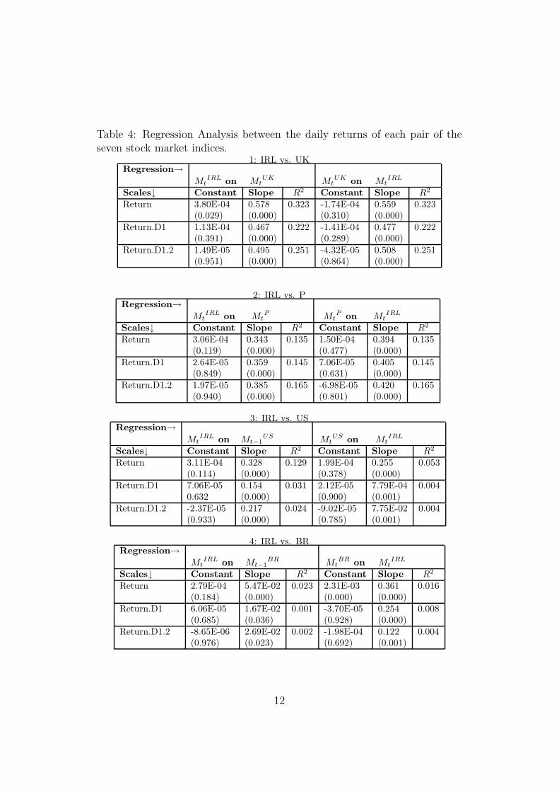
Table 4: Regression Analysis between the daily returns of each pair of theseven stock market indices.

1: IRL vs. UKRegression→

MtIRL on Mt

UK MtUK on Mt

IRL

Scales↓ Constant Slope R2 Constant Slope R2

Return 3.80E-04 0.578 0.323 -1.74E-04 0.559 0.323(0.029) (0.000) (0.310) (0.000)

Return.D1 1.13E-04 0.467 0.222 -1.41E-04 0.477 0.222(0.391) (0.000) (0.289) (0.000)

Return.D1.2 1.49E-05 0.495 0.251 -4.32E-05 0.508 0.251(0.951) (0.000) (0.864) (0.000)

2: IRL vs. PRegression→

MtIRL on Mt

P MtP on Mt

IRL

Scales↓ Constant Slope R2 Constant Slope R2

Return 3.06E-04 0.343 0.135 1.50E-04 0.394 0.135(0.119) (0.000) (0.477) (0.000)

Return.D1 2.64E-05 0.359 0.145 7.06E-05 0.405 0.145(0.849) (0.000) (0.631) (0.000)

Return.D1.2 1.97E-05 0.385 0.165 -6.98E-05 0.420 0.165(0.940) (0.000) (0.801) (0.000)

3: IRL vs. USRegression→

MtIRL on Mt−1

US MtUS on Mt

IRL

Scales↓ Constant Slope R2 Constant Slope R2

Return 3.11E-04 0.328 0.129 1.99E-04 0.255 0.053(0.114) (0.000) (0.378) (0.000)

Return.D1 7.06E-05 0.154 0.031 2.12E-05 7.79E-04 0.0040.632 (0.000) (0.900) (0.001)

Return.D1.2 -2.37E-05 0.217 0.024 -9.02E-05 7.75E-02 0.004(0.933) (0.000) (0.785) (0.001)

4: IRL vs. BRRegression→

MtIRL on Mt−1

BR MtBR on Mt

IRL

Scales↓ Constant Slope R2 Constant Slope R2

Return 2.79E-04 5.47E-02 0.023 2.31E-03 0.361 0.016(0.184) (0.000) (0.000) (0.000)

Return.D1 6.06E-05 1.67E-02 0.001 -3.70E-05 0.254 0.008(0.685) (0.036) (0.928) (0.000)

Return.D1.2 -8.65E-06 2.69E-02 0.002 -1.98E-04 0.122 0.004(0.976) (0.023) (0.692) (0.001)

12

5: IRL vs. JPRegression→

MtIRL on Mt

JP MtJP on Mt−1

IRL

Scales↓ Constant Slope R2 Constant Slope R2

Return 4.77E-04 0.181 0.068 -4.06E-04 0.127 0.007(0.019) (0.000) (0.183) (0.000)

Return.D1 5.16E-05 0.147 0.052 6.76E-05 -8.18E-02 0.002(0.723) (0.000) (0.771) (0.010)

Return.D1.2 -1.18E-05 0.147 0.054 2.61E-05 -0.115 0.002(0.996) (0.000) (0.954) (0.024)

6: IRL vs. HKRegression→

MtIRL on Mt

HK MtHK on Mt−1

IRL

Scales↓ Constant Slope R2 Constant Slope R2

Return 4.19E-04 0.183 0.104 -4.91E-05 3.86E-02 0.000(0.036) (0.000) (0.895) (0.292)

Return.D1 4.88E-05 0.170 0.097 9.54E-05 -0.302 0.028(0.731) (0.000) (0.724) (0.000)

Return.D1.2 -3.13E-06 0.182 0.117 -1.48E-05 -0.396 0.018(0.991) (0.000) (0.978) (0.000)

7: UK vs. PRegression→

MtUK on Mt

P MtP on Mt

UK

Scales↓ Constant Slope R2 Constant Slope R2

Return -7.95E-05 0.438 0.228 2.83E-04 0.521 0.228(0.663) (0.000) (0.155) (0.000)

Return.D1 -1.55E-04 0.451 0.224 1.51E-04 0.498 0.224(0.243) (0.000) (0.280) (0.000)

Return.D1.2 -1.22E-05 0.481 0.252 -4.86E-05 0.524 0.252(0.961) (0.000) (0.853) (0.000)

8: UK vs. USRegression→

MtUK on Mt−1

US MtUS on Mt

UK

Scales↓ Constant Slope R2 Constant Slope R2

Return -2.03E-05 0.251 0.078 2.78E-04 0.473 0.178(0.919) (0.000) (0.188) (0.000)

Return.D1 -1.12E-04 1.13E-02 0.000 5.54E-05 0.262 0.054(0.468) (0.537) (0.736) (0.000)

Return.D1.2 -4.73E-05 -3.46E-03 0.000 -7.70E-05 0.292 0.065(0.871) (0.906) (0.810) (0.000)

13

9: UK vs. BRRegression→

MtUK on Mt−1

BR MtBR on Mt

UK

Scales↓ Constant Slope R2 Constant Slope R2

Return -3.38E-05 3.71E-02 0.011 2.42E-03 0.659 0.054(0.870) (0.000) (0.000) (0.000)

Return.D1 -1.12E-04 -1.53E-02 0.001 3.49E-05 0.503 0.034(0.457) (0.057) (0.931) (0.000)

Return.D1.2 -4.76E-05 -1.38E-02 0.000 -1.86E-04 0.265 0.023(0.870) (0.250) (0.707) (0.000)

10: UK vs. JPRegression→

MtUK on Mt

JP MtJP on Mt−1

UK

Scales↓ Constant Slope R2 Constant Slope R2

Return 1.21E-04 0.178 0.068 -3.72E-04 0.292 0.039(0.548) (0.000) (0.214) (0.000)

Return.D1 -1.19E-04 0.113 0.030 5.73E-05 9.20E-02 0.003(0.423) (0.000) (0.805) (0.003)

Return.D1.2 -5.03E-05 0.124 0.037 2.42E-05 0.119 0.002(0.860) (0.000) (0.957) (0.018)

11: UK vs. HKRegression→

MtUK on Mt

HK MtHK on Mt−1

UK

Scales↓ Constant Slope R2 Constant Slope R2

Return 6.37E-05 0.187 0.112 -5.60E-05 0.349 0.038(0.745) (0.000) (0.879) (0.000)

Return.D1 -1.22E-04 0.133 0.058 7.07E-05 -4.37E-02 0.000(0.407) (0.000) (0.796) (0.239)

Return.D1.2 -4.39E-05 0.122 0.050 -3.17E-05 -6.80E-02 0.000(0.877) (0.000) (0.953) (0.257)

12: P vs. USRegression→

MtP on Mt−1

US MtUS on Mt

P

Scales↓ Constant Slope R2 Constant Slope R2

Return 2.59E-04 0.174 0.031 2.21E-04 0.265 0.067(0.246) (0.000) (0.323) (0.000)

Return.D1 9.76E-05 3.69E-02 0.001 9.36E-06 0.174 0.026(0.539) (0.055) (0.955) (0.000)

Return.D1.2 -7.64E-05 4.11E-02 0.000 -7.62E-05 0.199 0.033(0.801) (0.178) (0.815) (0.000)

14

13: P vs. BRRegression→

MtP on Mt−1

BR MtBR on Mt

P

Scales↓ Constant Slope R2 Constant Slope R2

Return 1.94E-04 4.94E-02 0.015 2.30E-05 0.489 0.035(0.391) (0.000) (0.000) (0.000)

Return.D1 9.52E-05 9.93E-03 0.000 -5.20E-05 0.319 0.015(0.549) (0.240) (0.899) (0.000)

Return.D1.2 -7.35E-05 6.73E-03 0.000 -1.85E-04 0.188 0.013(0.809) (0.590) (0.770) (0.000)

14: P vs. JPRegression→

MtP on Mt

JP MtJP on Mt−1

P

Scales↓ Constant Slope R2 Constant Slope R2

Return 3.60E-04 0.134 0.032 -4.00E-04 0.150 0.012(0.1060 (0.000) (0.188) (0.000)

Return.D1 8.83E-05 0.113 0.027 5.95E-05 4.06E-02 0.000(0.573) (0.000) (0.798) (0.203)

Return.D1.2 -7.62E-05 0.125 0.034 1.32E-05 6.50E-02 0.000(0.798) (0.000) (0.977) (0.174)

15: P vs. HKRegression→

MtP on Mt

HK MtHK on Mt−1

P

Scales↓ Constant Slope R2 Constant Slope R2

Return 3.19E-04 0.168 0.076 -7.77E-05 0.143 0.007(0.144) (0.0000 (0.834) (0.000)

Return.D1 8.53E-05 0.143 0.060 7.29E-05 -0.141 0.006(0.560) (0.000) (0.789) (0.000)

Return.D1.2 -6.90E-05 0.150 0.070 -1.34E-02 -0.130 0.002(0.814) (0.000) (0.980) (0.023)

16: US vs. BRRegression→

MtUS on Mt

BR MtBR on Mt

BR

Scales↓ Constant Slope R2 Constant Slope R2

Return -1.85E-05 0.132 0.110 2.20E-03 0.841 0.110(0.933) (0.000) (0.000) (0.000)

Return.D1 2.84E-05 0.114 0.076 -3.91E-05 0.674 0.077(0.861) (0.000) (0.921) (0.000)

Return.D1.2 -6.03E-05 0.154 0.054 -1.67E-04 0.351 0.054(0.852) (0.000) (0.732) (0.000)

15

17: US vs. JPRegression→

MtUS on Mt

JP MtJP on Mt−1

US

Scales↓ Constant Slope R2 Constant Slope R2

Return 3.31E-04 7.45E-02 0.009 -4.77E-04 0.401 0.092(0.152) (0.000) (0.101) (0.000)

Return.D1 2.92E-05 -5.37E-02 0.005 8.15E-05 0.322 0.056(0.862) (0.000) (0.718) (0.000)

Return.D1.2 -8.97E-05 -5.10E-02 0.004 -8.93E-06 0.441 0.041(0.991) (0.786) (0.994) (0.000)

18: US vs. HKRegression→

MtUS on Mt

HK MtHK on Mt−1

US

Scales↓ Constant Slope R2 Constant Slope R2

Return 3.07E-04 6.78E-02 0.011 -2.01E-04 0.541 0.114(0.184) (0.000) (0.566) (0.000)

Return.D1 2.97E-05 -5.50E-02 0.007 9.62E-05 0.401 0.063(0.860) (0.000) (0.719) (0.000)

Return.D1.2 -9.25E-05 -5.50E-02 0.008 -7.39E-05 0.630 0.058(0.779) (0.000) (0.888) (0.000)

19: BR vs. JPRegression→

MtBR on Mt

JP MtJP on Mt−1

BR

Scales↓ Constant Slope R2 Constant Slope R2

Return -5.34E-04 7.33E-02 0.019 2.51E-03 0.154 0.006(0.079) (0.000) (0.000) (0.000)

Return.D1 6.06E-05 5.79E-02 0.009 -2.31E-05 2.49E-02 0.000(0.794) (0.000) (0.955) (0.498)

Return.D1.2 2.16E-05 7.22E-02 0.006 -1.99E-04 4.43E-03 0.000(0.962) (0.000) (0.691) (0.848)

20: BR vs. HKRegression→

MtBR on Mt

HK MtHK on Mt−1

BR

Scales↓ Constant Slope R2 Constant Slope R2

Return -3.30E-04 0.121 0.036 2.46E-03 0.142 0.008(0.396) (0.000) (0.000) (0.000)

Return.D1 6.92E-05 9.99E-02 0.020 -2.03E-5 -1.85E-2 0.000(0.798) (0.000) (0.961) (0.554)

Return.D1.2 -3.03E-05 0.126 0.014 -1.99E-04 -9.94E-03 0.000(0.955) (0.000) (0.691) (0.609)

16

21: JP vs. HKRegression→

MtJP on Mt

HK MtHK on Mt

JP

Scales↓ Constant Slope R2 Constant Slope R2

Return -3.44E-04 0.283 0.119 1.16E-04 0.421 0.119(0.231) (0.000) (0.741) (0.000)

Return.D1 4.09E-05 0.284 0.111 4.54E-05 0.393 0.111(0.852) (0.000) (0.860) (0.000)

Return.D1.2 3.06E-05 0.297 0.126 -3.94E-05 0.424 0.126(0.942) (0.000) (0.938) (0.000)

Table 5: Regression Analysis between Portuguese and Brazilian Marketsusing three different scales

A: From 1993 To 1996Regression→

MtP on Mt−1

BR MtBR on Mt

P

Scales↓ Constant Slope R2 Constant Slope R2

Return 5.31E-04 1.36E-02 0.001 2.75E-03 5.54E-02 0.001(0.000) (0.401) (0.000) (0.430)

Return.D1 2.04E-07 -4.42E-02 0.010 -4.14E-07 0.139 0.003(0.999) (0.003) (0.999) (0.088)

Return.D1.2 7.95E-07 -6.37E-03 0.001 1.12E-07 -1.84E-02 0.001(0.996) (0.669) (1.000) (0.812)

B: From 1997 to 2000Regression→

MtP on Mt−1

BR MtBR on Mt

P

Scales↓ Constant Slope R2 Constant Slope R2

Return 5.28E-04 0.272 0.062 1.91E-04 0.270 0.085(0.222) (0.000)

Return.D1 7.95E-07 9.23E-02 0.010 -4.77E-07 0.136 0.016(0.998) (0.002) (0.999) (0.000)

Return.D1.2 1.87E-06 0.181 0.032 -7.47E-07 0.224 0.054(0.996) (0.000) (0.998) (0.000)

C: From 2001 To 2003Regression→

MtP on Mt−1

BR MtBR on Mt

P

Scales↓ Constant Slope R2 Constant Slope R2

Return -7.35E-04 0.259 0.041 2.40E-04 0.212 0.070(0.072) (0.000) (0.455) (0.001)

Return.D1 -2.16E-06 -1.95E-02 0.000 -4.42E-06 0.148 0.032(0.994) (0.677) (0.984) (0.000)

Return.D1.2 1.80E-06 0.164 0.016 -2.10E-06 0.184 0.048(0.996) (0.001) (0.994) (0.000)

17

where

• P-values of t-tests are given in parentheses.

• M IRL, MUK , MP , MUS , MBR, MJP and MHK are indicators of Irish, UK,Portuguese, US, Brazilian, Japanese and the Hong Kong market indices respectively.

• Return is an indicator of the row daily returns series.

• Return.D1 is an indicator of the returns series reconstructed by using the firstwavelet crystal.

• Return.D1+D2 is an indicator of the returns series reconstructed by using the firstand the second wavelet crystals together.

18

0 500 1000 1500 2000 2500

2000

3000

4000

5000

6000

Time

Pric

es

(a) ISEQ Overall index.

0 500 1000 1500 2000 2500

1500

2000

2500

3000

Pric

es

Time

Pric

es

(b) FTSE all share index.

0 500 1000 1500 2000 2500

4000

6000

8000

1000

012

000

1400

0

Time

Pric

es

(c) PSI20 index.

0 500 1000 1500 2000 2500

400

600

800

1000

1200

1400

Time

Pric

es

(d) S&P500 index.

19

0 500 1000 1500 2000 2500

050

0010

000

1500

0

Time

Pric

es

(e) Bovespa index.

0 500 1000 1500 2000 2500

1000

015

000

2000

0

Time

Pric

es

(f) Nikkei 225 index.

0 500 1000 1500 2000 2500

8000

1000

012

000

1400

016

000

1800

0

Time

Pric

es

(g) HSI index.

Figure 1: The daily prices from May 1st, 1993 to Septemeber 30th, 2003.

20

0 500 1000 1500 2000

s6

d6

d5

d4

d3

d2

d1

idwt

(a) ISEQ Overall index.

0 500 1000 1500 2000

s6

d6

d5

d4

d3

d2

d1

idwt

(b) FTSE all share index.

0 500 1000 1500 2000

s6

d6

d5

d4

d3

d2

d1

idwt

(c) PSI20 index.

0 500 1000 1500 2000

s6

d6

d5

d4

d3

d2

d1

idwt

(d) S&P500 index.

21

0 500 1000 1500 2000

s6

d6

d5

d4

d3

d2

d1

idwt

(e) Bovespa index.

0 500 1000 1500 2000

s6

d6

d5

d4

d3

d2

d1

idwt

(f) Nikkei 225 index.

0 500 1000 1500 2000

s6

d6

d5

d4

d3

d2

d1

idwt

(g) HSI index.

Figure 2: The discrete wavelet transform (DWT) of daily returns vs. Time.

22