Embed Size (px)
Citation preview

Interpreting neural population activity during feedback motor control
Submitted in partial fulfillment of the requirements for
the degree of
Doctor of Philosophy
in
Electrical and Computer Engineering
Matthew D. Golub
B.S., Electrical Engineering, Stanford University
M.S., Electrical Engineering, Stanford University
Carnegie Mellon University
Pittsburgh, PA
May, 2015

Thesis Committee:
Byron M. Yu, co-chair
Steven M. Chase, co-chair
Robert E. Kass
Tom M. Mitchell
ii

Abstract
The motor system routinely generates a multitude of fast, accurate, and elegant movements.
In large part, this capacity is enabled by closed-loop feedback control systems in the brain.
Brain-machine interfaces (BMIs), which translate neural activity into control signals for driv-
ing prosthetic devices, also engage the brain’s feedback control systems and offer a promising
experimental paradigm for studying the neural basis of feedback motor control. Here, we address
both the engineering challenges facing current BMI systems and the basic science opportunities
afforded by them.
Previous studies have demonstrated reliable control of the direction of movement in cursor-
based BMI systems. However, control of movement speed has been notably deficient. We pro-
vide an explanation for these observed difficulties based on neurophysiological studies of arm
reaching. These findings inspired our design of a novel BMI decoding algorithm, the speed-
dampening Kalman filter (SDKF) that automatically slows the cursor upon detecting changes
in decoded movement direction. SDKF improved success rates by a factor of 1.7 relative to a
standard Kalman filter in a closed-loop BMI task requiring stable stops at targets.
Next, we transition toward leveraging the BMI paradigm for basic scientific studies of feed-
back motor control. It is widely believed that the brain employs internal models to describe our
prior beliefs about how an effector responds to motor commands. We developed a statistical
framework for extracting a subject’s internal model from neural population activity. We discov-
ered that a mismatch between the actual BMI and the subjects internal model of the BMI explains
roughly 65% of movement errors. We also show that this internal model mismatch limits move-
ment speed dynamic range and may contribute toward the aforementioned known difficulties in
control of BMI movement speed.
iii

Acknowledgments
During my first visit to Carnegie Mellon, I was surprised to run into Byron Yu, who was
visiting as a faculty candidate. Although I had been working in the same Stanford lab where
Byron completed his graduate work and was wrapping up his post-doctoral work, neither of us
were aware the other’s travel plans that week. Over the next few years, I would joke that Byron
accepted Carnegie Mellon’s offer so that he could work with me. The truth, however, is that I
could not been more fortunate than to have the opportunity to work with Byron over the years to
come.
While I was eager to acquire the powerful repertoire of machine learning skills that Byron
brought to the world of neuroscience, Byron encouraged me to also learn the ways of experimen-
talists. This led me to meet Steve Chase, a post-doc at the time, who over the coming months
would mentor me in performing animal experiments, collecting neural data, and understanding
the limitations facing the brain-machine interfaces that we were working to improve. Steve,
Byron and I continued meeting regularly, developing the core ideas that would serve as the foun-
dation for my dissertation. Steve soon accepted a faculty position at Carnegie Mellon, which
meant I would have the privilege of having him officially co-advise me with Byron.
I am deeply thankful to Byron and Steve for their nurturing guidance over these past years.
They have taught me to ask impactful questions and to pursue elegant solutions. They have
inspired the design of powerful algorithms for data analysis, and they have coached me toward
effectively communicating our discoveries to audiences across a broad range of fields. I am
also grateful to Aaron Batista for welcoming me to participate in animal experiments within his
lab and for his passionate and insightful comments on manuscript drafts and practice talks; to
Rob Kass for his thoughtful advice and support throughout my years at Carnegie Mellon; and to
Andy Schwartz for inviting me to perform experiments in his lab and for collaborating through
our publication of that work. I also wish to thank Rob Kass and Tom Mitchell for their thought-
provoking questions as they served on my thesis committee along with Byron and Steve.
It has been a pleasure to work closely with a number of students and post-docs: Patrick
Sadtler, Kristen Quick, Will Bishop, Ben Cowley, Karthik Lakshmanan, Joao Semedo and Pete
Lund. I have also greatly enjoyed participating in our weekly Chase/Batista/Yu lab journal club,
iv

with its jovial crew of students and post-docs. I have received generous financial support from
the National Science Foundation’s Integrative Graduate Education and Research Traineeship
(IGERT) and from Carnegie Mellon’s Carnegie Institute of Technology through the Dean’s Fel-
lowship and the John and Claire Bertucci Graduate Fellowship. Byron has provided generous
support through his National Institute of Health (NIH) Collaborative Research in Computational
Neuroscience (CRCNS) grant from the National Institute of Child Health and Human Develop-
ment, and Steve has provided generous support through his Pennsylvania Department of Health
Commonwealth Universal Research Enhancement grant. Finally, none of this work would be
possible without the support of my family. Thank you Mom, Dad and Sarah for encouraging me
to follow my dreams with creativity and perseverance.
v

vi

Contents
1 Introduction 1
2 Previous work 5
2.1 Brain-machine interfaces . . . . . . . . . . . . . . . . . . . . . . . . . . . . . . 5
2.1.1 Neural recording systems . . . . . . . . . . . . . . . . . . . . . . . . . . 5
2.1.2 Prosthetic devices . . . . . . . . . . . . . . . . . . . . . . . . . . . . . . 6
2.1.3 Decoding algorithms . . . . . . . . . . . . . . . . . . . . . . . . . . . . 7
2.1.4 Current limitations . . . . . . . . . . . . . . . . . . . . . . . . . . . . . 9
2.2 BMIs for investigating the neural basis of feedback motor control . . . . . . . . . 10
2.3 Internal models . . . . . . . . . . . . . . . . . . . . . . . . . . . . . . . . . . . 11
2.3.1 Psychophysical studies of motor internal models . . . . . . . . . . . . . 12
2.3.2 Mechanistic studies of motor internal models . . . . . . . . . . . . . . . 13
2.3.3 Further neural correlates of motor internal models . . . . . . . . . . . . . 14
2.3.4 Internal models beyond the motor system . . . . . . . . . . . . . . . . . 14
3 Motor cortical control of movement speed with implications for brain-machine in-
terface control 17
3.1 Motivation . . . . . . . . . . . . . . . . . . . . . . . . . . . . . . . . . . . . . . 17
3.2 Results . . . . . . . . . . . . . . . . . . . . . . . . . . . . . . . . . . . . . . . . 18
3.2.1 Single-unit activity carries more information about direction than speed . 18
3.2.2 Population activity enables better predictions of direction than of speed . 25
3.2.3 Difficulties extracting speed may explain deficiencies in BMI control . . 31
vii
3.2.4 SDKF restores stopping ability during closed-loop BMI control . . . . . 33
3.3 Discussion . . . . . . . . . . . . . . . . . . . . . . . . . . . . . . . . . . . . . . 36
3.3.1 Information and prediction analyses: sensitivity to modeling choices . . . 37
3.3.2 Movement representations in motor cortex . . . . . . . . . . . . . . . . 38
3.3.3 Implications for brain-machine interface control . . . . . . . . . . . . . 41
3.4 Methods . . . . . . . . . . . . . . . . . . . . . . . . . . . . . . . . . . . . . . . 44
3.4.1 Neural recordings and behavioral tasks . . . . . . . . . . . . . . . . . . 44
3.4.2 Data discretization . . . . . . . . . . . . . . . . . . . . . . . . . . . . . 46
3.4.3 Optimization for direction discretization . . . . . . . . . . . . . . . . . . 47
3.4.4 Information analysis . . . . . . . . . . . . . . . . . . . . . . . . . . . . 48
3.4.5 Simulated neural populations . . . . . . . . . . . . . . . . . . . . . . . . 50
3.4.6 Linear regression analysis . . . . . . . . . . . . . . . . . . . . . . . . . 51
3.4.7 Neural decoding for arm reaching . . . . . . . . . . . . . . . . . . . . . 52
3.4.8 Neural decoding for BMI control . . . . . . . . . . . . . . . . . . . . . 54
3.4.9 Simulated closed-loop control of movement . . . . . . . . . . . . . . . . 58
4 Internal models for interpreting neural population activity during sensorimotor
control 61
4.1 Motivation . . . . . . . . . . . . . . . . . . . . . . . . . . . . . . . . . . . . . . 61
4.2 Results . . . . . . . . . . . . . . . . . . . . . . . . . . . . . . . . . . . . . . . . 62
4.2.1 Internal models underlie BMI Control . . . . . . . . . . . . . . . . . . . 64
4.2.2 Internal model mismatch explains the majority of subjects’ control errors 67
4.2.3 Internal model mismatch explains limitations in speed dynamic range . . 76
4.2.4 Perturbations drive internal model adaptation . . . . . . . . . . . . . . . 79
4.2.5 Controls for validation of the IME framework . . . . . . . . . . . . . . . 82
4.3 Discussion . . . . . . . . . . . . . . . . . . . . . . . . . . . . . . . . . . . . . . 87
4.4 Methods . . . . . . . . . . . . . . . . . . . . . . . . . . . . . . . . . . . . . . . 90
4.4.1 Neural recordings . . . . . . . . . . . . . . . . . . . . . . . . . . . . . . 90
4.4.2 Behavioral task . . . . . . . . . . . . . . . . . . . . . . . . . . . . . . . 90
4.4.3 The BMI mapping . . . . . . . . . . . . . . . . . . . . . . . . . . . . . 92
viii

4.4.4 Calibration of the BMI mapping . . . . . . . . . . . . . . . . . . . . . . 93
4.4.5 Error metrics for assessing estimates of movement intent . . . . . . . . . 94
4.4.6 Characterizing inherent visuomotor latencies . . . . . . . . . . . . . . . 95
4.4.7 Assessing feedback delay compensation . . . . . . . . . . . . . . . . . . 97
4.4.8 Framework for internal model estimation . . . . . . . . . . . . . . . . . 98
4.4.9 Variants on the IME framework . . . . . . . . . . . . . . . . . . . . . . 102
4.4.10 Parameter fitting for the IME framework . . . . . . . . . . . . . . . . . 104
4.4.11 Internal model estimation as an inverse optimal control problem . . . . . 106
4.4.12 Comparing predictions between the internal model and the BMI mapping 114
4.4.13 Visualizing an extracted internal model . . . . . . . . . . . . . . . . . . 114
4.4.14 Evaluating the speed bias resulting from internal model mismatch . . . . 115
5 Summary and future directions 117
6 Appendix A. Collaborative work 121
Bibliography 123
ix

x

List of Figures
3.1 Information curves for 40 representative units . . . . . . . . . . . . . . . . . . . 20
3.2 Information maximizing lags for speed and direction . . . . . . . . . . . . . . . 22
3.3 MDI and MSI for a representative dataset . . . . . . . . . . . . . . . . . . . . . 23
3.4 Within-unit MDI vs MSI for simulated datasets . . . . . . . . . . . . . . . . . . 24
3.5 Linear regression analysis of the same 40 units from Fig. 3.1 . . . . . . . . . . . 26
3.6 Evaluation of PNB predictions . . . . . . . . . . . . . . . . . . . . . . . . . . . 27
3.7 PNB prediction accuracy as a function of the number of units . . . . . . . . . . . 30
3.8 Example BMI cursor trajectories from successful trials . . . . . . . . . . . . . . 32
3.9 Cursor speed under VKF control as a function of distance to target center . . . . 32
3.10 Success rate as a function of target hold requirement for BMI experiments . . . . 33
3.11 Comparison of BMI control under SDKF and VKF . . . . . . . . . . . . . . . . 34
3.12 Angular velocity as a function of cursor-to-target distance for SDKF and VKF . . 35
3.13 RMSE for offline SDKF- and VKF-based decoding of arm movements . . . . . . 36
3.14 Discretization of movement kinematics . . . . . . . . . . . . . . . . . . . . . . 47
3.15 Speed-dampening as a function of the most recent angular velocity . . . . . . . . 59
4.1 Schematic view of the brain-machine interface . . . . . . . . . . . . . . . . . . . 63
4.2 Closed-loop control of a BMI cursor . . . . . . . . . . . . . . . . . . . . . . . . 63
4.3 Proficient control of the BMI . . . . . . . . . . . . . . . . . . . . . . . . . . . . 64
4.4 Subjects compensate for sensory feedback delays while controlling a BMI . . . . 66
4.5 Evidence of an internal model revealed through perturbation of the BMI mapping 67
4.6 Internal model mismatch explains the majority of cursor movement errors . . . . 70
4.7 Neural activity is consistently correct through the internal model . . . . . . . . . 71
xi

4.8 IME whiskers consistently point to the target: additional example trials . . . . . . 71
4.9 Errors from trials in Figure 4.8 highlighted on the distribution of errors across trials 73
4.10 Low-dimensional illustration comparing an internal model to the BMI mapping . 74
4.11 Internal models explain cursor errors across all types of trials . . . . . . . . . . . 75
4.12 A comparison of the subject’s internal model and the BMI mapping . . . . . . . 76
4.13 Internal model mismatch limits the dynamic range of BMI cursor speeds . . . . . 78
4.14 An example of internal model mismatch limiting cursor speed dynamic range . . 79
4.15 Extracted internal models capture adaptation to perturbations . . . . . . . . . . . 83
4.16 IME’s explanatory power comes primarily from structure in the neural activity . . 84
4.17 IME does not identify structure in the high-dimensional neural activity when no
such structure exists . . . . . . . . . . . . . . . . . . . . . . . . . . . . . . . . . 85
4.18 A simplified alternative internal model is not consistent with the data . . . . . . . 86
4.19 Error metrics for assessing estimates of movement intent . . . . . . . . . . . . . 96
4.20 Full probabilistic graphical model for the IME framework . . . . . . . . . . . . . 101
4.21 Example trials overlaid with pIME whiskers . . . . . . . . . . . . . . . . . . . . 103
4.22 Model selection in for determining the feedback delay, τ . . . . . . . . . . . . . . 105
4.23 gIME graphical model with a single timestep feedback delay (τ = 1). . . . . . . 110
xii

List of Tables
3.1 Numbers of units with significant MDI and MSI . . . . . . . . . . . . . . . . . . 21
3.2 Frequencies of units with significantly greater MDI than MSI and vice versa . . . 23
3.3 PNB classification accuracies for speed and direction across all datasets . . . . . 28
xiii

xiv

Chapter 1
Introduction
The motor system routinely generates a multitude of fast, accurate, and elegant movements. In
large part, this capacity is enabled by closed-loop feedback control systems in the brain. These
systems continuously integrate multiple modalities of sensory information to form internal rep-
resentations of the dynamic state of the body. Task demands combine with these feedback-
mediated body representations to generate motor output from the brain. Although much is known
about how sensory information is encoded and how motor commands drive movements, rela-
tively little is known about how these sensory and motor systems coordinate to give rise to a
robust feedback control system.
It has been difficult to directly study the neurophysiology of feedback motor control due to
the massive numbers of neurons participating in control, the nonlinear dynamics in much of the
musculoskeletal system, the multiple contributing modalities of sensory feedback, and the lack of
an appropriate statistical framework for reconciling these complexities. Brain-machine interfaces
(BMIs) provide a simplified feedback control system, within which it becomes tractable to more
directly study the neural basis of closed-loop motor control. In particular, in a BMI, all neural
activity that directly drives the device is recorded, the dynamics of the device can be chosen by
the experimenter, and feedback can be limited to a single modality (e.g., vision). These features
of the BMI paradigm provide the experimenter with unprecedented access to the motor system
and facilitate novel studies of feedback motor control and motor learning.
Brain-machine interfaces (BMIs) have traditionally been developed for assisting disabled
1

patients by translating neural activity into control signals for driving prosthetic devices, such as
a robotic limb or a computer cursor. In Chapter 2, we provide a literature survey of previous
work related to BMI systems and feedback motor control. We then present the contributions of
this dissertation, which address both the engineering challenges facing current BMI systems and
the basic science opportunities afforded by BMI systems. On the engineering side, we develop
solutions for understanding and advancing the performance of intracortical BMI systems. For
the purposes of basic neuroscience, we develop novel statistical tools and analyses of neural
population activity underlying feedback motor control.
The first contribution of this dissertation addresses a longstanding limitation to BMI perfor-
mance. The clinical viability of BMI systems depends critically on achievable performance.
While previous studies have demonstrated reliable control of the direction of movement in
cursor-based BMI systems, control of movement speed has been notably deficient. In Chap-
ter 3, we examine the motor cortical coding of movement speed in an effort to determine the
bottleneck underlying this deficiency in BMI speed control. We then develop a novel BMI de-
coding algorithm using a radical approach informed by our study of the motor cortical code.
Finally, we describe a series of closed-loop BMI experiments that I conducted to validate this
decoding algorithm.
Next, we transition toward leveraging the BMI paradigm for basic scientific studies of feed-
back motor control. During control of limb movements, the brain continuously takes in sensory
information about the limb, internally tracks the state of the limb, and produces appropriate mo-
tor commands. It is widely believed that this process is enabled by an internal model, which
describes our prior beliefs about how the limb responds to motor commands. We begin Chapter
4 with a validation of BMI as a paradigm for studying internal models by demonstrating that
BMI movements engage internal models, just as reaching movements do. With this evidence
that internal models underlie BMI control, we continue to extract a rich representation of an in-
ternal model. Most previous studies of internal models have been based upon low-dimensional
behavioral measurements or recordings from individual neurons. As such, it has been difficult to
identify a rich internal model that accounts for both observed behavior and neural activity. We
propose a novel statistical framework for extracting a subject’s internal model in unprecedented
2

detail from high-dimensional neural population activity. Specifically, we consider the inverse
optimal control problem of learning a subject’s internal model from demonstrations of control
and knowledge of task goals. We develop a probabilistic framework and exact EM algorithm
to jointly estimate the subject’s internal model, the subject’s internal predictions about the BMI
cursor state, and the subject’s visual feedback delay. In the main results of Chapter 4, we harness
extracted internal models as a lens through which to interpret neural population activity.
Finally, in Chapter 5, we summarize the main contributions of this dissertation and propose
research directions that may be enabled by the contributions of this dissertation. The contribu-
tions of this dissertation have been published or submitted for publication as follows:
Chapter 3
Golub, M. D., Yu, B. M., Schwartz, A. B., and Chase, S. M. (2014). Motor cortical control of
movement speed with implications for brain-machine interface control. Journal of neurophysi-
ology, 11:(411-429).
Chapter 4
Golub, M. D., Yu, B. M., and Chase, S. M. (2012). Internal models engaged by brain-computer
interface control. In 34th International Conf. of the IEEE Engineering in Medicine and Biology
Society, pages 1327-1330.
Golub, M. D., Chase, S. M., and Yu, B. M. (2013). Learning an internal dynamics model from
control demonstration. In Proceedings of The 30th International Conference on Machine Learn-
ing, pages 606-614 (24% acceptance rate).
Golub M. D., Yu B. M., and Chase S. M. (2015). Internal models for interpreting neural popula-
tion activity during sensorimotor control. Under review.
3

Appendix A
In addition to these contributions, Appendx A briefly describes a collaborative project that has
been published as follows:
Sadtler P. T., Quick K. M., Golub M. D., Chase S. M., Ryu S. I., Tyler-Kabara E. C., Yu B. M.,
and Batista A. P. (2014). Neural constraints on learning. Nature, 512:(423-426).
4

Chapter 2
Previous work
2.1 Brain-machine interfaces
Brain-machine interfaces (BMIs) translate neural activity into control signals for driving pros-
thetic devices. In doing so, BMIs aim to restore the capacity for movement and communication
in patients with neurodegenerative diseases, spinal cord injuries, or limb amputations. A BMI
is composed of i) a system for recording neural activity from the brain, ii) a prosthetic device
to be controlled by the recorded neural activity, and iii) a decoder to map the recorded neural
activity into commands that drive the prosthetic device. In the following section, we provide a
brief literature survey for each of these components of the BMI system.
2.1.1 Neural recording systems
BMIs rely on extracting signals related to movement intent from the brain (Andersen et al., 2004;
Waldert et al., 2009). Neural activity can be monitored using a number of technologies, from
the minimally invasive functional magnetic resonance imaging (Lee et al., 2009), magnetoen-
cephalography (Georgopoulos et al., 2005), and electroencephalography (McFarland et al., 1997;
Millan et al., 2004), to the more-invasive electrocorticography (Schalk and Leuthardt, 2011) and
intracortical electrode recordings. Intracortical recordings made extracellularly can resolve neu-
ronal spiking activities with a high signal-to-noise ratio, and as such, this is the recording tech-
nology underlying state-of-the-art BMI systems. Olds (1965) and Fetz (1969) demonstrated the
5

earliest proofs-of-concept that modulation of single neuron responses could be operantly condi-
tioned through rewards that were tied to feedback of neural firing. Current BMI systems rely
on volitional modulation of many neurons recorded simultaneously using chronically implanted
arrays of extracellular electrodes.
To extract movement-related signals, recording electrodes in BMI systems most often target
the primary motor cortex (M1). Activity in M1 has been shown to encode information about
many kinematic variables, including movement direction (Georgopoulos et al., 1982; Schwartz
et al., 1988; Ashe and Georgopoulos, 1994) and movement speed (Schwartz, 1992, 1994; Moran
and Schwartz, 1999b; Churchland et al., 2006). The parietal reach region (PRR) of posterior
parietal cortex and the dorsal premotor cortex (PMd) have been shown to encode high-level
movement goals (Batista et al., 1999; Messier and Kalaska, 2000). BMIs have also been demon-
strated based on recordings from these areas (Musallam et al., 2004; Santhanam et al., 2006).
The cerebellum and subcortical regions, such as the thalamus and the basal ganglia, also partici-
pate in the generation of movement (Alexander et al., 1986), but are more difficult to access and
thus are not typically considered for BMI applications.
2.1.2 Prosthetic devices
Intracortical BMIs have been designed to drive a range of prosthetic devices. In arguably the
earliest demonstration of a motor cortical BMI, Fetz (1969) conditioned monkeys to modulate the
activity of single neurons in the primary motor cortex (M1) by reinforcing particular firing rates
with food rewards and by providing feedback in the form of audible clicks or visual deflections
of a voltage meter. In this case, the prosthetic devices are the reward and feedback systems.
Prosthetic control of a robotic arm was introduced by Chapin et al. (1999), who trained rats
to drive movement of a simple robotic arm by modulating the activity of recorded neurons in M1
and ventrolateral thalamus. Wessberg et al. (2000) and Carmena et al. (2003) demonstrated that
monkeys could learn BMI control of robotic arms with 2-3 degrees-of-freedom (DOF). Velliste
et al. (2008) then demonstrated that monkeys could modulate neural activity to drive 4 DOFs of
a robotic arm in a self-feeding task involving interaction of the robot with both the food rewards
and the subjects themselves. Studies with human subjects have begun to translate progress from
6

these rat and monkey studies into demonstrations of clinical viability of intracortical BMIs for
driving robotic limbs (Hochberg et al., 2006, 2012; Collinger et al., 2013).
In addition to driving robotic limbs, BMIs have been used to drive continuous movements
of computer cursors (Serruya et al., 2002; Taylor et al., 2002; Mulliken et al., 2008a; Suminski
et al., 2010; Gilja et al., 2012) and to select from a discrete set of targets (Musallam et al., 2004;
Santhanam et al., 2006). Functional electrical stimulation of intact limb muscles has also been
driven by a recent BMI in monkeys (Ethier et al., 2012). Progress has also been made toward
locomotion-based BMIs in studies of rats (Song et al., 2009) and monkeys (Fitzsimmons et al.,
2009).
2.1.3 Decoding algorithms
A decoding algorithm provides the critical link between the neural recordings and the prosthetic
device (Brockmeier and Prıncipe, 2013). Its purpose is to predict the intended state of the pros-
thetic device based on the available neural recordings. In the case of a prosthetic cursor, the
state typically includes the current cursor position, and may also include higher-order kinematic
derivatives (e.g., velocity, acceleration). In the case of a robotic arm, the state must include a
sufficient set of variables to specify the arm configuration. For discrete communications BMIs,
the state is an element from a pre-specified set (e.g., a letter on a keyboard or an icon from a
computer desktop). Decoding algorithms make different assumptions about how neural activity
relates to the intended state of the prosthesis, and these assumptions in turn specify the form and
parameterization of the prediction.
One approach to decoder design is to impose minimal assumptions about the neural activ-
ity and to directly learn a mapping from neural activity to prosthetic commands. Wiener filters
(WFs) (Carmena et al., 2003; Serruya et al., 2002) and artificial neural networks (Chapin et al.,
1999) fall into this category. An alternative approach is to assume that firing rates systematically
reflect specific parameters of a movement and can be described by an encoding or observation
model. Once fit, this model can then be mathematically inverted into a decoding model. A
prominent example is the cosine tuning model, which is inverted to define the population vector
algorithm (PVA) (Georgopoulos et al., 1982). Here, each neuron is modeled as firing maximally
7

when movement is in a particular preferred direction, and firing rate decreases (following a co-
sine curve) as the angle increases between the direction of movement and the preferred direction.
When the recorded neurons’ preferred directions are not uniformly distributed, PVA leads to a
biased estimate of movement direction, which is compensated by instead using the optimal linear
estimator (OLE) to invert the tuning curves (Salinas and Abbott, 1994).
Movements tend to have statistical regularities, which are not reflected by the algorithms
described thus far. For example, movement velocity tends to change smoothly across time. This
notion can be captured by a probabilistic trajectory or state-transition model, describing how
the state is expected to evolve from one timestep to the next. When the trajectory model is
Markov (i.e., the current state depends only on the previous tilmestep’s state), and when both the
observation and trajectory models are linear-Gaussian, an optimal state estimate is given by the
Kalman filter (KF) (Kalman, 1960). Kalman filters have been used extensively in BMI systems
(Wu et al., 2006; Kim et al., 2008; Mulliken et al., 2008a; Gilja et al., 2012; Orsborn et al., 2014).
Collectively, the WF, PVA, OLE and KF are referred to as linear estimators because the estimated
movement state, or “decode,” can be expressed as a linear function of the neural activity and (in
the case of the KF) the previous estimates.
More sophisticated decoding algorithms are required when modeling assumptions include
nonlinear relationships or non-Gaussian noise. An example of a nonlinear observation model is
one that models the expected observed firing rate of a neuron using independent contributions
from both intended scalar speed and intended vector velocity (Li et al., 2009b). Because speed
is the magnitude (a nonlinear transformation) of velocity, no linear model can express such a
relationship. An important example of a non-Gaussian noise model is the Poisson noise model,
which is particularly well-suited for modeling spike counts because its support is the set of non-
negative integers (i.e., it models a distribution of counts) and because it models noise variance as
being tied to mean firing rate (i.e., matching empirical observations in recorded spiking activity).
A number of estimation algorithms have been developed to allow for decoding under these less-
restrictive modeling assumptions. The particle filter (Brockwell et al., 2004) uses a stochastic
sampling approach toward inferring a desired movement state, whereas the Laplace-Gaussian
filter (Koyama et al., 2010a) and unscented Kalman filter (Li et al., 2009a) perform inference
8

using deterministic approximations. These filters are collectively referred to as nonlinear estima-
tors because their estimates cannot be expressed as linear functions. Although their underlying
model assumptions often better match the statistics of recorded neural and behavioral data, it is
not clear that they offer higher-performance relative to linear methods when incorporated into
closed-loop BMI systems (Koyama et al., 2010b).
2.1.4 Current limitations
Despite impressive advances in BMI technologies in recent years, BMI control of cursors and
robotic limbs is still inferior to able-bodied control of natural limbs and physical pointing devices,
especially with respect to the stability of stopping, as pointed out in previous studies (Carmena
et al., 2003; Hochberg et al., 2006; Kim et al., 2008; Ganguly and Carmena, 2009; Gilja et al.,
2012). One possible performance bottleneck might be that current BMI systems can only record
from relatively small populations of neurons. With access to larger populations, decoding algo-
rithms might better dissociate movement-related signals from noise. Another possibility is that
current decoding algorithms might not be maximally utilizing the available neural populations.
Most decoding algorithms solve some type of estimation problem. While an algorithm may be
optimal in the estimation sense (i.e., it may minimize error when reconstructing movements of-
fline), it might not be optimal for closed-loop control. Chase et al. (2009) showed that, despite the
fact that PVA is known to produce biased directional estimates, subjects are able to compensate
in a closed-loop setting such that, for each BMI cursor target, the direction of cursor movements
under the PVA appears nearly identical to the direction of movements decoded in closed-loop by
the unbiased OLE.
Several recent studies have begun to address the discrepancy between offline estimation and
closed-loop control. Gilja et al. (2012) designed a modified Kalman filter that incorporates the
assumption that the subject knows the current BMI cursor position (e.g., from available visual
feedback and possible use of an internal model), and that applies closed-loop decoder adapta-
tion under the assumption that the subject intends to drive the BMI cursor straight toward the
target from that cursor position. In a related study, Orsborn et al. (2014) showed that neural
adaptation can occur simultaneously with closed-loop decoder adaptation to yield improved task
9

performance across days. It may be possible to further improve BMI performance by designing
systems that align synergistically with subjects’ abilities to adapt (Sadtler et al., 2014; Shenoy
and Carmena, 2014).
2.2 BMIs for investigating the neural basis of feedback motor
control
In addition to their promising clinical applications, BMIs offer a simplified and well-defined
feedback control system, which facilitates the study of the neural basis of feedback motor control.
In particular, the BMI system offers substantial simplifications to several key complexities of
native limb control. First, native limb control involves effectors with non-linear dynamics, and
the causal relationship between the recorded neural activity and limb movements is not fully
specified in the experiment. In contrast, the causal relationship between recorded neural activity
and BMI cursor movements is completely specified by the experimenter and can be chosen to
be linear. Second, native limb control involves multiple modalities of sensory feedback (e.g.,
proprioception and vision), which makes it difficult for the experimenter to know exactly what
information is known to the subject and at what time. In the BMI, task-relevant sensory feedback
is limited to a single modality (vision), and its content and timing are completely specified by
the experimenter. Finally, the neural activity that drives the BMI is completely specified by the
recorded population activity, whereas typically only a subset of neurons driving limb movements
is recorded.
These features of BMI systems have led experimenters toward adopting BMI as a paradigm
for exploring the neural substrates of feedback motor control. Early BMI studies, despite fo-
cusing on technological development, found that BMI control is a skill that improves with ex-
perience (Taylor et al., 2002; Carmena et al., 2003). Ganguly and Carmena (2009) designed a
study in which subjects controlled a BMI cursor across many days using a single decoder and
a stable population of recorded M1 cells. They found that patterns of neural activation became
increasingly stereotyped across days, suggesting that subjects had developed and refined an in-
ternal model of the BMI system. Ganguly et al. (2011) followed-up with a comparison between
10

recorded cells that were directly linked to the BMI and other “indirect” cells that were simultane-
ously recorded, but did not directly contribute to BMI cursor movements. This analysis revealed
that firing rates of the indirect cells decreased their depths of modulation to cursor movements
relative to those of the direct cells, suggesting that, over many days, an internal model can be
learned for specific subpopulations of cells.
2.3 Internal models
A substantial portion of this dissertation is dedicated toward identifying and studying internal
models of the BMI. Here we provide a brief survey of the literature surrounding internal models.
An internal model can be defined loosely to be as a set of prior beliefs encoded in the brain
that mediates perception of sensory events or guides motor actions. Internal models have been
widely studied across a wide range of species, including electric fish (Requarth and Sawtell,
2014; Requarth et al., 2014; Kennedy et al., 2014), insects (Webb, 2004; Mischiati et al., 2015),
songbirds (Keller and Hahnloser, 2009), monkeys (Sommer and Wurtz, 2002; Komatsu, 2006;
Ghasia et al., 2008; Mulliken et al., 2008b; Laurens et al., 2013), and humans (Wolpert et al.,
1995; Komatsu, 2006; Shadmehr and Krakauer, 2008; Shadmehr et al., 2010). These studies
address internal models across multiple sensory systems, including electrosensory (Requarth
and Sawtell, 2014; Requarth et al., 2014; Kennedy et al., 2014), visual (Komatsu, 2006; Berkes
et al., 2011), and vestibular (Laurens et al., 2013) systems, and across multiple motor systems,
including flight (Mischiati et al., 2015), vocalization (Keller and Hahnloser, 2009), oculomotor
(Sommer and Wurtz, 2002; Green et al., 2007; Ghasia et al., 2008) and skeletomotor (Shadmehr
and Mussa-Ivaldi, 1994; Wolpert et al., 1995; Mulliken et al., 2008b; Shadmehr and Krakauer,
2008) systems.
In the motor system, an internal forward model contains those prior beliefs necessary for pre-
dicting the sensory consequences of a motor command (Jordan and Rumelhart, 1992; Wolpert
et al., 1995; Miall and Wolpert, 1996; Desmurget and Grafton, 2000; Mehta and Schaal, 2002;
Frens and Donchin, 2009). In an arm reaching context, a forward model could predict the up-
coming arm configuration given the previous arm configuration and internal copies of recently
11

issued motor commands. An internal inverse model is typically defined as a mapping from a de-
sired movement into a motor command (or sequence of motor commands) that would implement
the desired movement (Kawato et al., 1987; Wolpert and Kawato, 1998; Mussa-Ivaldi and Bizzi,
2000; Sabes, 2000). Both types of motor internal models incorporate one’s inner conceptions
about the physics of the effector and how neural commands drive movements of the effector. For
successful motor control, the forward and inverse models should be well-tuned to each other and
to the effector being controlled.
Why do we need internal models? Even simple movements, like reaching to grasp a glass
of water, require dozens of muscles to be activated with precise coordination. This precision
is especially impressive in light of sensory feedback delays inherent to neural transmission and
processing: when we make a swift arm movement, the brain only knows where the arm was a split
second ago, not where it currently is. The latency between visual stimuli and neural responses
in M1 is on the order of 100 ms in primates (Schwartz et al., 1988). For rapid online error
correction, a forward model is essential in that it enables an internal prediction of the current
effector state before the corresponding sensory feedback becomes available, thus facilitating
compensation for sensorimotor delays. From a computational standpoint, it should be noted
that these internal state predictions need not be explicitly computed to produce output motor
commands that compensate for system delays. Rather, compensatory motor commands could be
directly computed from sensory feedback and internal copies of previous motor commands.
2.3.1 Psychophysical studies of motor internal models
Much evidence supporting the brain’s use of internal models comes from human psychophysi-
cal studies demonstrating behavioral correlates of internal models. Wolpert et al. (1995) asked
subjects to estimate the endpoint of perturbed and visually obscured hand movements. They
found that localization errors were well-described by a framework that incorporated both pro-
prioceptive sensory inflow as well as internal state estimation via an internal forward model
that integrates motor outflow. Shadmehr and Mussa-Ivaldi (1994) showed that, when arm move-
ments are perturbed by a viscous force field, subjects adapt with experience until arm movements
appear nearly identical to those prior to the perturbation. When the perturbation was removed,
12

aftereffects in the arm movements indicated that compensation for the perturbation was mediated
by an adaptive and persistent internal model, rather than by compensatory increases in muscle
stiffness. Thoroughman and Shadmehr (2000) further investigated adaptation to viscous force
fields in arm reaching movements and found that removal of the force field for just a single trial
resulted in predictable “unlearning” in subjects’ internal models.
The cerebellum is believed to subserve computations of an internal forward model for mo-
tor control. Behavioral evidence comes from cerebellar patients who present reaching deficits
consistent with an inability to internally predict the outcome of motor commands and thus to
compensate for sensory feedback delays (Shadmehr and Krakauer, 2008; Bhanpuri et al., 2013).
In healthy subjects, Miall et al. (2007) applied transcranial magnetic stimulation to the cere-
bellum during sequential arm reaches and found that movements became biased in a manner
consistent with a disrupted ability to internally track the arm.
2.3.2 Mechanistic studies of motor internal models
In parallel to these psychophysical studies, mechanistic studies have made important progress
toward identifying the neural circuits that implement internal models. As a motor command is
issued from the brain to the muscles, it is believed than an internal copy of the command, often
referred to as efference copy or corollary discharge, is sent in parallel to an internal forward
model, which predicts the command’s sensory consequences. Sommer and Wurtz (2002) identi-
fied this internal copy pathway in the macaque saccadic eye movement system, in a relay from
the superior colliculus to the frontal eye field through mediodorsal thalamus. When the thalamic
relay was reversibly inactivated, sequential eye movements exhibited biases consistent with an
inability to internally track the initial eye movement in the sequence (similar to the behavioral
effect reported by Miall et al. (2007)). Also studying macaque eye movements, Ghasia et al.
(2008) suggested that eye-head (EH) neurons in the brainstem carry a forward prediction signal,
and nearby burst tonic (BT) cells carry an internal copy of the eye movement command. The crit-
ical distinction was that EH cells represented the torsional component of eye movements, which
is a consequence of the mechanics of the extraocular muscles and is not directly driven by ocular
motor neurons. BT cells represented eye motion, but not its torsional component. For reach-
13

ing movements, recent evidence suggests that cervical propriospinal neurons (CPNs) may carry
the analogous internal copy command. This class of neurons carries projections downstream to
motor neurons that innervate forelimb muscles and upstream to the cerebellum via the lateral
reticular nucleus (LRN) (Alstermark and Ekerot, 2013). Azim et al. (2014) found that reach-
ing was impaired in mice when optical stimulation disrupted the internally directed upstream
pathway from CPNs to LRN.
2.3.3 Further neural correlates of motor internal models
In addition to these mechanistic studies, which largely focus on the inputs to a forward model, a
limited number of studies have taken the complementary approach of investigating neurophysio-
logical links between behavior and putative outputs of an internal model. Mulliken et al. (2008a)
found that individual neurons in posterial parietal cortex represented movements of a joystick,
but at lags too soon to represent motor outflow but too late to represent sensory inflow. They
claimed that these neurons represented the internal predictions of a forward model. Gribble and
Scott (2002) studied monkeys making reaching movements with external loads introduced at var-
ious positions on the arm. From recordings of individual neurons in M1, they found that neural
activity from multiple-load movements could be predicted from neural activity during move-
ments with each individual load, suggesting that internal models subserving simple movements
can be combined to form a basis for driving complex movements.
2.3.4 Internal models beyond the motor system
Although we have focused on reviewing the literature surrounding internal models for the motor
system, much related work has been done in identifying internal models across various sensory
systems. Rather than guiding movement, these internal models drive perception by integrating
sensory stimuli with prior beliefs about the statistics of sensory events. In the vestibular sys-
tem, cerebellar Purkinje cells have been shown to resolve ambiguities in bodily accelerations
(Green et al., 2005; Laurens et al., 2013). In the visual system, internal models are believed to
subserve perceptual filling-in (Komatsu, 2006). During development, internal models driving
14

visual cortical activity are believed to adapt to the statistical properties of the visual environment
(Berkes et al., 2011). In the electrosensory system of weakly electric fish, internal models have
been shown to compensate for self-induced electric fields (Requarth and Sawtell, 2014; Requarth
et al., 2014; Kennedy et al., 2014). In the mouse auditory system, internal models are believed to
inform auditory-guided behaviors by driving movement-related modulation of auditory process-
ing (Schneider et al., 2014).
15

16

Chapter 3
Motor cortical control of movement speed
with implications for brain-machine
interface control
3.1 Motivation
Previous studies have investigated the extent to which motor cortex encodes kinematic vari-
ables, including movement direction (Georgopoulos et al., 1982; Schwartz et al., 1988; Ashe and
Georgopoulos, 1994) and movement speed (Schwartz, 1992, 1994; Moran and Schwartz, 1999b;
Churchland et al., 2006). The ability to accurately read out direction and speed from motor cortex
takes particular importance in the context of brain-machine interfaces (BMIs), which translate
neural activity into control signals for driving prosthetic devices, such as robotic limbs (Chapin
et al., 1999; Wessberg et al., 2000; Carmena et al., 2003; Velliste et al., 2008) or computer cur-
sors (Serruya et al., 2002; Taylor et al., 2002; Mulliken et al., 2008a; Suminski et al., 2010; Gilja
et al., 2012). Despite impressive advances in BMI technologies in recent years, BMI control of
cursors and robotic limbs is still inferior to able-bodied control of natural limbs and physical
pointing devices, especially with respect to the stability of stopping, as pointed out in previous
studies (Carmena et al., 2003; Hochberg et al., 2006; Kim et al., 2008; Ganguly and Carmena,
2009; Gilja et al., 2012). To better understand the origin of this poor control of BMI movement
17

speed, we looked for signatures of a robust representation of instantaneous movement speed in
single-trial reaching movements.
We analyzed spike trains recorded simultaneously across primary and premotor cortices
of rhesus monkeys during a 3D center-out reaching task. Using standard information theo-
retic and population decoding techniques, we found substantially less speed-related informa-
tion than direction-related information in neural activity at the levels of both single units and
simultaneously-recorded populations. We also performed a unit-dropping analysis, which sug-
gests that our ability to decode movement speed might not improve substantially with access to
larger numbers of neurons. None of our analyses revealed a substantial representation of the
moment-by-moment details of movement speed on single-trial bases.
The finding that speed information is difficult to extract from motor cortical population ac-
tivity informed a novel approach to implementing movement speed when driving BMI devices.
This decoder, termed the speed-dampening Kalman filter (SDKF), incorporates the assumption
that movement speed and angular velocity should be inversely related. Rather than relying on
neural activity to provide the complete details of movement speed, which may be difficult to
extract in the real-time setting of BMI, SDKF enhances control of movement speed using direc-
tional signals, which are more easily extracted from neural activity. Since movement direction
can be reliably inferred from motor cortical population responses, angular velocity (the temporal
derivative of direction) can be extracted reliably as well. SDKF uses angular velocity of the de-
coded cursor trajectory to modulate cursor speed, thus reducing the system’s reliance on cortical
activity to directly provide the moment-by-moment details of movement speed.
3.2 Results
3.2.1 Single-unit activity carries more information about direction than
about speed
To characterize the speed-related and direction-related information carried by spike trains from
individual neural units, we computed the mutual information between neural activity and move-
18

ment kinematics. Mutual information is a statistic describing the extent of dependence between
two random variables. In contrast to correlation coefficients determined from linear regression,
mutual information does not require specifying a form for the relationship between two variables,
allowing it to capture arbitrary nonlinear relationships if they are indeed present in the data.
Movement speed and direction are continuous-valued quantities expressed using different
units and numbers of degrees-of-freedom. To enable an unbiased comparison of the relationships
between neural activity and these two kinematic quantities, we discretized movement speed and
direction such that their statistical properties were matched (see Section 3.4.2).
For each unit we determined the lag at which mutual information was maximized between
spike counts and lagged discretized direction, τdirection, and lagged discretized speed, τspeed,
where positive lags correspond to causal relationships between neural activity and movement
kinematics. Henceforth we refer to the mutual information at these optimal lags as maximal
direction information (MDI) and maximal speed information (MSI).
Spike trains from single units contained speed- and direction-related information in a variety
of forms. Figure 3.1 shows speed and direction information as a function of lag for a number of
representative units. Direction information curves were unimodal for nearly every recorded unit,
whereas it was not uncommon for speed information curves to be bimodal. These bimodal speed
information curves are likely a reflection of task-induced autocorrelation in movement speed
(e.g., through bell-shaped speed profiles). Most units’ maximal direction information (MDI) and
maximal speed information (MSI) were significant relative to null information levels, although
some units were exceptions, as detailed in Table 3.1. The number of units with significant MDI
was larger than the number of units with significant MSI for all 9 experiments.
Figure 3.2 shows the lags at which each unit achieved its MDI and MSI. Optimal lags for
direction information were most often causal, meaning information-carrying spikes tended to
lead movement direction. Optimal lags for speed-related information were casual and acausal in
roughly equal frequencies. Many units thus had substantial discrepancies between their optimal
direction and speed lags, and, on average, optimal direction lags were more positive (i.e., causal)
than optimal speed lags within individual units.
Perhaps most striking, however, were the differences between MDI and MSI values within
19

▽▽
**▽
▽ ▽▽
**▽
▽
▽
**▽▽ ▽▽ ▽▽
**▽
▽
**
▽ ▽ ▽▽
▽▽ **▽
▽
**▽
▽
**
▽
▽**
▽ ▽▽**
▽▽
▽
**▽
▽
**▽▽
**▽
▽▽
▽ ▽ ▽
**▽
▽ ▽▽ ▽ ▽
▽▽**
▽▽
**▽
**
▽▽ ▽▽
−300 0 3000
0.15
0.3
▽▽
acausal causal
lag, τ (ms)
info
rmat
ion
(b
its)
▽▽
acausal causal
▽▽
**▽▽
**▽
▽
**▽▽
**▽
▽
Figure 3.1: Information curves for 40 representative units from a single experiment (F081909).
Mutual information between spike counts and movement direction (blue) or movement speed
(red) was computed as a function of time lag between neural activity and kinematics. Triangles
indicate lags at which maximal direction information (MDI) and maximal speed information
(MSI) were achieved and were omitted if those information values were not significantly greater
than expected by chance (permutation test, p < 0.001). For positive lags, neural activity led
kinematics in the information calculation. Shaded regions represent 95% confidence intervals
(bootstrap). At top right of each panel, ** denotes MDI>MSI (blue) or MSI>MDI (red) (boot-
strap, p < 0.001).
20
Dataset speed and direction direction only speed only neither total units
F081309 99 (83) 10 (8) 5 (4) 5 (4) 119
F081709 98 (82) 10 (8) 6 (5) 5 (4) 119
F081809 95 (80) 11 (9) 5 (4) 8 (7) 119
F081909 95 (80) 14 (12) 8 (7) 2 (2) 119
T110410 43 (66) 10 (15) 1 (2) 11 (17) 65
T110510 53 (69) 15 (19) 1 (1) 8 (10) 77
T110910 50 (61) 18 (22) 3 (4) 11 (13) 82
T111010 38 (58) 16 (24) 1 (2) 11 (17) 66
T111210 34 (69) 5 (10) 4 (8) 6 (12) 49
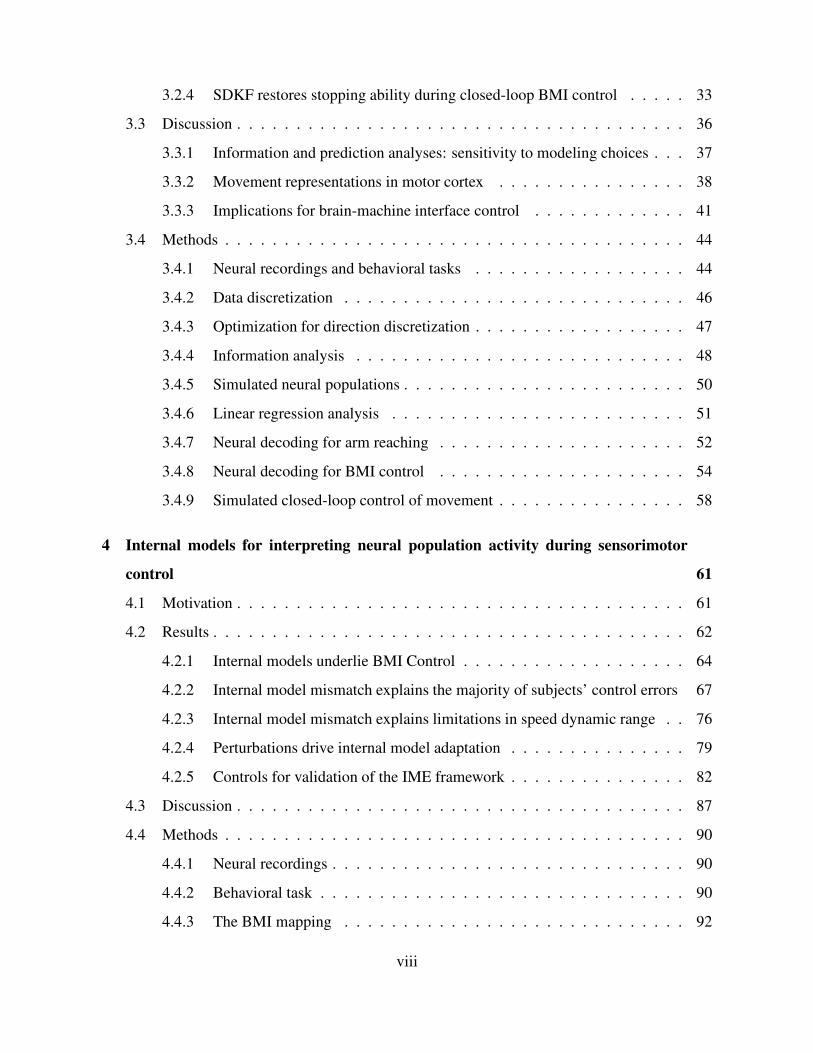
Table 3.1: Numbers of units with significant maximal direction information (MDI) and speed
information (MSI) across all recorded units from each experiment. Percentages of total units are
given in parentheses.
individual units. Of 119 units from a representative dataset (F081809), 45 (38%) had MDI values
that were significantly greater than their MSI values, while only 12 (10%) showed the opposite
relation (Fig. 3.3A). Consistent with this breakdown, we found significantly more direction-
related information than speed-related information on average across all recorded units with
significant differences in MDI and MSI from this dataset (Fig. 3.3B). This breakdown of unit-
types was consistent across datasets from both subjects, with 3.01±0.63 times as many direction-
dominated cells as speed-dominated cells (see Table 3.2). For all Monkey F datasets, average
MDI was significantly greater than average MSI (p < 0.001, right-tailed t-test). For Monkey T
datasets, average MDI was always greater than average MSI, but due to lower unit counts, these
differences were statistically significant for only 3 of 5 datasets (p < 0.05, right-tailed t-test).
To aid in interpreting this uneven breakdown of direction- versus speed-encoding units, we
simulated spike counts from four relevant encoding models: direction-only; speed-only; veloc-
ity (i.e., ); and independent speed and direction. We fit each model to the neural activity and
raw movement kinematics (non-discretized) from the representative dataset (F081909) and then
simulated spike counts using the same real kinematics. As expected, when simulating from the
direction-only encoding model, no units were identified with MSI significantly greater than MDI
(Fig. 3.4A), and similarly, when simulating from the speed-only encoding model, no units were
identified with MDI significantly greater than MSI (Fig. 3.4B). The information pattern from the
velocity-encoding population (Fig. 3.4C) resembled that from the direction-only population, but
21

since speed is a fundamental component of velocity, MSI values were slightly larger in the veloc-
ity encoding population. Even so, none of these simulated units had an MSI that was significantly
larger than its corresponding MDI.
The information signature from the simulated speed-and-direction encoding population (Fig. 3.4D)
best resembled that of the real data (Fig. 3.3A), with a large number of units with significantly
greater MDI than MSI in addition to a small number of units showing the opposite trend. This
similar breakdown of direction- versus speed-dominated units should be expected since the data
were generated from a model fit to the real data. The direction-only, speed-only and velocity
encoding models result in theoretically prescribed distributions of MDI and MSI values. This
−300 −200 −100 0 100 200 300
−300
−200
−100
0
100
200
300
τspeed
(ms)
τ dir
ecti
on (
ms)
0
10
20
30 causalacausal
τspeed
(ms)
# u
nit
s
causal
acausal
# units
τd
irection (m
s)
0 10 20 30
Figure 3.2: Information maximizing lags for speed and direction from a representative dataset
(F081909). Positive lags correspond to neural activity leading kinematics (i.e., causal). Fre-
quency histograms of optimal lags for speed and direction are shown in top and right panels,
respectively. Units were omitted if either their speed or direction information was not statisti-
cally significant.
22

A
0 0.1 0.2 0.3
0
0.1
0.2
0.3
MSI (bits)
MD
I (b
its)
B
−0.2 −0.1 0 0.1 0.2
0
10
20
30**
MDI − MSI (bits)
# u
nit
s
Figure 3.3: MDI and MSI for a representative dataset (F081909). (A) Within-unit MDI vs MSI.
Units with significantly different MDI and MSI values (bootstrap, p < 0.001) are shown in blue
(MDI greater) and red (MSI greater). Units with no significant difference between MDI and
MSI are shown in black. (B) Frequency histogram of within-unit differences between MDI and
MSI for units with significantly different MDI and MSI (i.e., excluding units from (A) denoted
in black). On average (dashed line), MDI was significantly larger than MSI (p = 5.2 × 10⁻⁶,
one-sided t-test).
Dataset MDI > MSI MSI > MDI total units
F081309 41 (34) 11 (9) 119
F081709 40 (34) 13 (11) 119
F081809 40 (34) 15 (13) 119
F081909 45 (38) 12 (10) 119
T110410 15 (23) 7 (11) 65
T110510 26 (34) 7 (9) 77
T110910 29 (35) 9 (11) 82
T111010 25 (38) 9 (14) 66
T111210 12 (24) 6 (12) 49
Table 3.2: Frequencies of units with significantly greater MDI than MSI and vice versa (p <0.001, bootstrap). Percentages of total units are given in parenthesis.
distribution for the independent speed and direction model, however, can favor either direction
or speed unit types, depending on the data. Also, note that the distributions of MDI and MSI
values from these simulations are biased toward slightly smaller values than those from the real
data in Fig. 3.3A. These differences speak to the fact that the real neural activity contains move-
ment information not captured by the parametric tuning models used in these simulations (as
23

A
0 0.1 0.2 0.3
0
0.1
0.2
0.3
MSI (bits)
MD
I (b
its)
Simulated dataDirection−only model
B
0 0.1 0.2 0.3
0
0.1
0.2
0.3
MSI (bits)
MD
I (b
its)
Simulated dataSpeed−only model
C
0 0.1 0.2 0.3
0
0.1
0.2
0.3
MSI (bits)
MD
I (b
its)
Simulated dataVelocity model
D
0 0.1 0.2 0.3
0
0.1
0.2
0.3
MSI (bits)
MD
I (b
its)
Simulated dataIndep. speed anddirection model
Figure 3.4: Within-unit MDI vs MSI for datasets simulated from (A) direction-only, (B) speed-
only, (C) velocity, and (D) independent speed and direction encoding models. Same format and
scale as Fig. 3.3A.
observeded, for example, by Churchland and Shenoy (2007)), yet this information is captured by
the mutual information computations employed over the real neural data in this analysis.
To establish a link between this information analysis motor cortical tuning, we also performed
a linear regression analysis (Georgopoulos et al., 1982; Schwartz, 1992; Ashe and Georgopoulos,
1994; Lebedev et al., 2005; Perel et al., 2013). We fit regression models that assumed recorded
spike counts encoded kinematics through direction-only tuning, speed-only tuning, or velocity
tuning. Tuning indices (TI), defined as√R2 from fits to these regression models, are shown
in Fig. 3.5 as a function of lag between kinematics and neural activity. Direction TI curves
closely matched the direction information curves of Fig. 3.1, and similarly speed TI curves
24

closely matched the speed information curves. Velocity TI curves typically had maxima that
exceeded both the corresponding speed and direction TI maxima (although a few exceptions can
be found). These velocity TI curves were more closely matched to the TI and information curves
of direction than of speed, but did not appear to be a simple function of one or the other. We
note that TI values for direction and velocity are not directly comparable to those for speed due
to differences in numbers of parameters between models and because TI values were computed
over the same data used to fit the models. Rather, this analysis was motivated to 1) help carry
over intuition from previous studies framed from a regression perspective, and 2) to demon-
strate that the appearance of velocity tuning does not necessarily predict the quantity of speed-
or direction-related information that may be extracted from a population.
3.2.2 Population activity enables better predictions of direction than of
speed
Results from the information analysis suggests that, at least in single-unit activity, the encod-
ing of movement speed is substantially weaker than that of movement direction. To determine
whether this finding holds true when considering the joint population activity, we applied a series
of Poisson naıve Bayes classifiers toward predicting kinematics from simultaneously recorded
population responses. Classifiers were trained to predict discretized kinematics based on (i) a
single 30 ms spike count aligned in time with movement kinematics (instantaneous), or (ii) the
entire causal history of non-overlapping 30 ms spike counts beginning 300 ms before the move-
ment kinematics (history). Direction predictions were significantly more accurate than speed
predictions under both the instantaneous and history conditions and across all datasets. For the
representative dataset detailed in previous sections (F081909), instantaneous direction accuracy
was 26.0%, while speed accuracy was only 9.8%, as shown in Figs. 3.6A and 3.6G. Incorporat-
ing spike count history into predictions for this dataset increased direction accuracy to 38.7%,
while speed accuracy only increased to 13.1%. While these prediction accuracies may seem low
on an absolute scale, they are actually relatively high given that predictors had to choose from
26 possible labels for both speed and direction, and as such, chance prediction accuracy was
only 3.8%. These trends were consistent across all datasets, with direction accuracy 2.34± 0.25
25

−300 0 3000
0.3
0.6 acausal causal
lag, τ (ms)
tun
ing
in
dex
Figure 3.5: Linear regression analysis of the same 40 units from Fig. 3.1. Tuning indices, de-
fined as√R2 from linear regressions, are shown for direction-only (blue), speed-only (red) and
velocity (black) tuning models (Eqs. 3.10, 3.11, and 3.12, respectively).
times higher than speed accuracy for instantaneous predictions and 2.80± 0.23 times higher for
predictions based on spike count history. Prediction accuracies for all datasets are tabulated in
Table 3.3.
To summarize the full distribution of predictions, we also computed mutual information be-
tween predicted and actual discretized kinematics. As shown in Figs. 3.6B and 3.6H, direction
predictions carried more information than did speed predictions. As a performance metric, infor-
mation complements prediction accuracy in that information provides a summary of the structure
of predictions, including both the predictions that matched the actual kinematics as well as those
26

A
0
15
30
45
**p
red
icti
on
acc
ura
cy (
%)
direction speed
G
0
15
30
45**
pre
dic
tio
n a
ccu
racy
(%
)
direction speed
B
0
0.5
1
1.5
2
info
rmat
ion
(b
its)
direction speed
H
0
0.5
1
1.5
2
info
rmat
ion
(b
its)
direction speed
C
pre
dic
ted
actual direction
D
pre
dic
ted
actual speed
I
pre
dic
ted
actual direction
J
pre
dic
ted
actual speed
E
pre
dic
ted
(reo
rder
ed)
actual direction
F
pre
dic
ted
(reo
rder
ed)
actual speed
K
pre
dic
ted
(reo
rder
ed)
actual direction
L
pre
dic
ted
(reo
rder
ed)
actual speed
fraction
of p
redictio
ns (%
)
45
0
fraction
of p
redictio
ns (%
)
65
0
Figure 3.6: Evaluation of PNB predictions on dataset F081909. (A)-(F) evaluate predictions
based on a single 30 ms spike count aligned in time with kinematics. (A) Prediction accuracy.
Error bars indicate 95% confidence intervals (Bernoulli process, ** denotes p < 0.001), and
dashed line indicates chance prediction accuracy. (B) Information between predicted and ac-
tual kinematics labels. Dashed lines indicate null information computed as mean information
between actual labels and 200 shuffled sets of actual labels. (C)-(D) Confusion matrices for di-
rection and speed predictions, respectively. The jth column gives the distribution of predicted
kinematics given that the actual kinematics had label j. Each column is normalized to sum to
100%. (E)-(F) Confusion matrices from (C)-(D) with the rows of each column sorted by angle
(direction) or absolute difference (speed) between kinematics corresponding to actual and pre-
dicted labels. Correct predictions are shown along the diagonal in (C)-(D) and as the top row in
(E)-(F). (G)-(L) evaluate predictions based on causal history of spike counts in the same format
as (A)-(F).
that did not. Specifically, if two sets of predictions have the same fraction of correct predictions,
information will be higher for the set whose incorrect predictions are less uniformly distributed
across labels. In this regard, information can appropriately account for near misses, for example,
if a classifier frequently predicts an incorrect label corresponding to a speed that is only slightly
27

Instantaneous History
Monkey Dataset # unitsDir. acc. Speed acc. Dir. acc.
Speed acc.
Dir. acc. Speed acc. Dir. acc.Speed acc.(%) (%) (%) (%)
F 081309 119 26.3 10.5 2.5 38.8 11.4 3.4
F 081709 119 25.8 9.2 2.8 35.8 11.5 3.1
F 081809 119 24.9 9.3 2.7 36.0 12.8 2.8
F 081909 119 26.0 9.8 2.7 38.7 13.1 3.0
T 110410 65 17.3 7.5 2.3 29.8 10.0 3.0
T 110510 77 17.1 6.8 2.5 28.0 11.0 2.5
T 110910 82 17.2 6.8 2.5 29.2 10.7 2.7
T 111010 66 15.2 7.1 2.1 27.4 9.8 2.8
T 111210 49 13.2 7.0 1.9 24.8 10.1 2.5
Table 3.3: PNB classification accuracies for speed and direction across all datasets. Instantaneous
predictions are based on 30 ms spike counts time-aligned with kinematics. History predictions
are based on a 300 ms causal history of spike counts in non-overlapping 30 ms bins. Chance
prediction accuracy is 3.8% for instantaneous and history predictions of both speed and direction.
higher than the speed corresponding to the true label.
Confusion matrices are shown in Fig. 3.6c,d and Fig. 3.6i,j. While adjacent speed labels
correspond to adjacent speed ranges, no such natural ordering exists for three-dimensional di-
rections. To compensate, we provide column-reordered confusion matrices in Fig. 3.6e,f and
Fig. 3.6k,l, whereby the rows in each column have been sorted by angle (direction) or absolute
difference (speed) between kinematics corresponding to actual and predicted labels. The confu-
sion matrices show that incorrect prediction labels typically clustered around the correct label for
both speed and direction. These distributions were tighter for direction than for speed, resulting
in greater information values for direction than for speed.
We chose to include causal neural activity as the input to classifiers to mimic the real-time
prediction problem that a BMI is required to solve. However, the information analysis revealed
maximal speed information at acausal lags for many units (Fig. 3.2). When repeating the decod-
ing analysis using both the causal and acausal histories of neural activity, we found prediction
accuracies were largely unchanged as compared to the corresponding accuracies using only ca-
sual neural activity.
To ensure that our discretization procedure is not responsible for these discrepancies between
direction and speed prediction accuracies, we analyzed speed prediction accuracies as a function
28

of speed bin widths used for discretization. For predictions based on instantaneous spike counts,
there was never a significant effect of bin width on prediction accuracy. For predictions based
on spike count history, bin width had a small, but significant effect on 2 of 9 analyzed datasets;
however, these 2 experiments had low unit counts relative to the other experiments.
To determine the effect of population size on prediction accuracy, we performed a unit-
dropping analysis. As expected, predictions become more accurate with increased population
size for both movement speed and movement direction (Fig. 3.7A). We note that the confidence
intervals in the latter portion of the neuron-dropping curves (i.e., for numbers of units approach-
ing the actual recorded population size) will be biased to be smaller than they actually are due
to the similarity across draws from the actual population. However, even when accounting for
this, extrapolation of these accuracy curves beyond the numbers of units we recorded suggests
that, had we recorded a larger sample of neurons, speed prediction accuracy would likely remain
substantially lower than that of direction predictions (data not shown).
We also computed PNB prediction accuracy as a function of the number of contributing units
for simulated population recordings (Figs. 3.7B–3.7E). Consistent with the single-unit informa-
tion analyses, the independent speed and direction encoding model resulted in a population with
PNB prediction accuracies best matched to those of the real data. The key corresponding fea-
tures are (i) the ratio of direction-to-speed prediction accuracy across population size, and (ii)
the nearly saturated speed prediction accuracy when all units are incorporated into predictions.
However, this simulated population gives systematically lower prediction accuracies for both
speed and direction relative to those given by the real recorded data. This discrepancy again
speaks to the fact that the real recorded neural data contains movement information not captured
by the parametric tuning models used for these simulations, and that PNB classifiers are capable
of extracting this information from neural activity.
As described, the information and prediction analyses have treated speed and direction sep-
arately, characterizing each kinematic variable’s relationship to neural activity independent of
the other variable. We also performed the prediction analysis using a joint discretization scheme
whereby classifiers were trained to jointly predict speed and direction from each of 262 possible
pairs of discretized speeds and directions. Because these classifiers required learning many more
29

A
0 50 100
0
5
10
15
20
25
30
# units
pre
dic
tio
n a
ccu
racy
Real dataB
0 50 100
0
5
10
15
20
25
30
# units
pre
dic
tio
n a
ccu
racy
Simulated dataDirection−only model
C
0 50 100
0
5
10
15
20
25
30
# units
pre
dic
tio
n a
ccu
racy
Simulated dataSpeed−only model
D
0 50 100
0
5
10
15
20
25
30
# units
pre
dic
tio
n a
ccu
racy
Simulated dataVelocity model
E
0 50 100
0
5
10
15
20
25
30
# units
pre
dic
tio
n a
ccu
racy
Simulated dataIndep. speed anddirection model
Figure 3.7: PNB prediction accuracy for speed (red) and direction (blue) as a function of the
number of units contributing to predictions. For the 119-unit case, there is only one unique
combination of all 119 units. For the one-unit and 118-unit case, there are 119 unique unit
combinations. In these cases, prediction accuracies were computed for all possible unit combi-
nations. For each intermediate number of units, 1000 randomly selected unit combinations were
assessed. Colored lines and shaded regions represent median accuracies and 95% of accuracies
thereabout, respectively. Black lines indicate chance prediction accuracies. (A) Real data from
experiment F081909. (B) Simulated data from the direction-only encoding model. (C) Simulated
data, speed-only model. (D) Simulated data, velocity model. (E) Simulated data, independent
speed and direction model.
parameters, some datasets were not large enough to support the analysis. For the datasets that
were large enough, marginal prediction accuracies for direction were again significantly greater
than those for speed, although overfitting of the increased numbers of parameters produced abso-
lute accuracies that were slightly lower than those reported in our main results (data not shown).
To mitigate overfitting, we restricted the analysis to in-plane trials and decreased the number
of speed and direction bins to 8 each. This joint decoding analysis was well defined for all
datasets and produced similar results to an analogous analysis where speed and direction were
30

each decoded independently (data not shown).
3.2.3 Difficulties extracting speed may explain deficiencies in BMI control
Previous BMI studies have noted subjects’ difficulties in controlling BMI cursor speeds, espe-
cially with respect to stopping and holding a cursor at a desired target location (Carmena et al.,
2003; Hochberg et al., 2006; Kim et al., 2008; Ganguly and Carmena, 2009; Gilja et al., 2012).
To align with these studies, we implemented a BMI cursor control task using a velocity-only
Kalman filter (VKF), a state-of-the-art neural decoder for BMI applications. Example cursor
trajectories under VKF are shown in Fig. 3.8, as well as in Suppl. Video 1. During experimental
sessions when all trials had minimal target hold requirements (50 ms), cursor trajectories were
swift and straight into the targets (Fig. 3.8A). To quantify the subject’s ability to crisply stop at
targets, we introduced substantial hold requirements, such that trial success required the cursor
to overlap the target for a randomized hold time (0-600 ms), and a trial was failed if the cur-
sor exited this acceptance region during the hold time. During these experimental sessions with
substantial target hold requirements, the subject demonstrated poor control of movement speed
under VKF, as evidenced by frequent trial failures due to overshooting through the target (Suppl.
Video 1). Successful trials often involved meandering trajectories (Fig. 3.8B), such that cursor
speed was relatively low upon initial acquisition of the target. When target hold requirements
were minimal, this meandering behavior was not observed, and cursor speeds were substantially
higher upon target acquisition (Fig. 3.9), suggesting that the subject adopted a VKF-specific
strategy whereby stable stops were replaced by slow movements over the target. Consistent with
this strategy, the subject’s performance under VKF decreased substantially as target hold time
requirements increased (Fig. 3.11A).
We have shown that (i) in single-trial arm reaches, speed information is relatively deficient in
motor cortical activity compared to the abundant levels of direction information, and (ii) motor
cortical activity alone cannot support precise control of BMI cursor stability under VKF. Several
studies have highlighted the differences between closed-loop BMI control and offline analyses
of arm control (Lebedev et al., 2005; Chase et al., 2009). To establish a link between the ap-
parent deficiency of speed information offline and deficient speed control online, we simulated
31

VKF50 ms hold req.
A
VKF300−600 ms hold req.
B
SDKF300−600 ms hold req.
C
Figure 3.8: Example BMI cursor trajectories from successful trials. Dark circles show target
sizes as displayed during experiments. Light circles denote cursor-target overlap zones that take
into account the cursor radius (not shown). (A) VKF control with minimal target hold require-
ments (dataset F072310). (B) VKF control with target hold requirements between 300-600 ms
(dataset F062810). (C) SDKF control with target hold requirements between 300-600 ms (dataset
F062810).
50 ms hold req.
300−600 ms hold req.
0 20 40 60 80
0
50
100
150
200
distance to target (mm)
spee
d (
mm
/s)
Figure 3.9: Cursor speed under VKF control as a function of distance to target center when target
hold requirements were 50 ms (dashed gray line) and during separate sessions when target hold
requirements were 300-600 ms (solid gray line). Target acquisition began 14 mm from target
center (dashed black line). Data shown for successful trials only.
closed-loop BMI control as decoded by VKF. The underlying simulated neural population had
log-linear tuning to the independent speed and direction model (Eq. 3.8), which was fit to real
recorded neural activity from the arm reaching experiments. Thus the simulated population en-
coded substantially more information about desired direction than about desired speed. As shown
in Fig. 3.10, simulated control was consistent with the real VKF BMI behavioral data in that suc-
32

0 100 200 300 400 500 600
0
50
100
succ
ess
rate
(%
)
hold requirement (ms)
Figure 3.10: Success rate as a function of target hold requirement for real BMI experiments
under VKF control (solid line) and for simulated BMI control (dashed line). Error bars indicate
95% confidence intervals (Bernoulli process).
cess rates decreased rapidly as target hold requirements increased. This result suggests that the
amount of speed information found during arm movements is consistent with the subject’s de-
ficient ability to hold at targets, and further, that the amount of speed information required for
stable stopping under VKF BMI control exceeds the amounts that we found in recorded motor
cortical activity.
3.2.4 SDKF restores stopping ability during closed-loop BMI control
From the information and prediction analyses, we found our ability to extract speed-related infor-
mation from motor cortical activity to be relatively poor, despite using methods that require only
mild assumptions about how movement speed might be encoded in neural activity. The resulting
implication for BMI is that, even if it were possible to perfectly extract the limited speed infor-
mation available in recorded neural activity, this may never enable reliable closed-loop control
of BMI cursor speed because the encoding for movement speed is simply not that strong.
We designed the speed-dampening Kalman filter (SDKF) to overcome this limitation in the
decodability of movement speed. SDKF leverages the subject’s reliable control of movement
direction to improve control of movement speed by implementing a tradeoff between speed and
angular velocity in the decoded velocity signal. When cursor trajectories exhibit large absolute
angular velocities, SDKF constrains decoded speeds to be closer to zero in a graded fashion
depending on the magnitude of the angular velocity. In this manner, straight movements can be
fast, and curved or corrective movements can be used to slow the cursor.
33

A
0 100 200 300 400 500 600
0
50
100
succ
ess
rate
(%
)
* ** ****
**
VKF
SDKF
B
0 100 200 300 400 500 600
0
0.5
1
1.5
hold requirement (ms)
mo
vem
ent
tim
e (s
) *
Figure 3.11: Comparison of BMI control under SDKF (black) and VKF (gray). (A) Success
rate as a function of target hold requirement for all trials where an initial target acquisition was
achieved. VKF data are replicated from Fig. 3.10. Trials were deemed failures and terminated if
the cursor exited the target region before the hold requirement was satisfied. Error bars indicate
95% confidence intervals (Bernoulli process; ** denotes p < 0.001; * denotes p < 0.01). (B)
Movement times, defined as the elapsed time between target onset and initiating the target hold
period, as a function of target hold requirement for all successful trials. Error bars denote ± one
standard error (* denotes p < 0.01, Wilcoxon test).
Example cursor trajectories under SDKF are shown in Fig. 3.8C, as well as in Suppl. Video 2.
SDKF significantly enhanced the subject’s ability to stop and hold for the duration of target hold
requirements, as shown in Fig. 3.11A. For target hold times between 300-600 ms, success rates
were 1.7 times higher under SDKF control than under VKF control. Cursor movements under
SDKF were typically straight toward the target, rather than meandering (Fig. 3.8), indicating that
the subject could instruct a crisp stop upon acquiring the target. We applied a constant speed
gain to decoded SDKF velocities such that movement times were matched between VKF and
SDKF trials (Fig. 3.11B). In this setting, SDKF achieved improved cursor stability at targets
with movement times that were not significantly different from VKF movement times for hold
requirements longer than 100 ms (for hold requirements under 100 ms, movements did not need
to slow down substantially at targets to achieve task success).
SDKF improves BMI performance by leveraging natural features of goal-directed move-
34

ments, as well as by potentially encouraging strategies specific to the feedback equations defin-
ing SDKF. Goal-directed movements, in both natural reaching and BMI settings, tend to begin
with a high-speed, straight ballistic phase and tend to end with low-speed corrective movements
relying heavily on sensory feedback. SDKF detects these corrective movements in the form of
increased angular velocity, and correspondingly slows or stops the BMI cursor. This feature of
SDKF is akin to a “hockey stop,” whereby a fast moving hockey player makes a quick rotation
of his skates to bring about a crisp stop upon the ice. For SDKF, the result is a BMI cursor
that automatically slows down near the target in response to corrective movements, in contrast to
the overshooting behavior typically produced by standard BMI decoders. Figure 3.12 shows de-
coded angular velocity for SDKF and VKF as a function of distance to target. For both decoders,
angular velocities are low during the ballistic phase when the cursor is far from the target, and
as the cursor approaches the target, angular velocities increase. Interestingly, SDKF trajectories
showed larger angular velocities near the target compared to VKF, suggesting that the subject
may have adopted a strategy of exaggerating turns near the target because doing so would be
decoded by SDKF as a crisp “hockey stop.”
SDKF was designed to improve online BMI control of cursor speed. However, SDKF’s per-
formance benefits for online control, especially those that may be attributable to SDKF-specific
0204060
0
90
180
270
360
450**
**
*
distance to target (mm)
abso
lute an
gu
lar velo
city (d
egrees/
s)
Figure 3.12: Absolute angular velocity, |ωt|, as a function of cursor-to-target distance for SDKF
(black) and VKF (gray). Error bars denote ± one standard error (** denotes p < 0.001; * denotes
p < 0.01, Wilcoxon test). For each distance value, absolute angular velocities were first averaged
within each trial, and then a mean and standard error were computed across trials.
35
0
20
40
60
80**
dec
od
ing
err
or
(mm
/s)
SDKF VKF
Figure 3.13: Root-mean-squared errors for offline SDKF- and VKF-based decoding of arm
movements. Errors were first averaged within each trial, and then a mean and standard error
were computed across trials. Error bars denote ± one standard error. SDKF-decoding error was
significantly greater than VKF-decoding error (p = 3.2−20, one-sided t-test).
control strategies, need not result in improved performance when reconstructing arm movements
offline. We applied both SDKF and VKF toward offline reconstruction of arm velocity, and found
root-mean-squared reconstruction error to be nearly twice as large for SDKF relative to VKF
(Fig. 3.13). This result highlights the fact that decoding algorithms with superior performance
in online cursor control do not necessarily achieve superior performance in offline reconstruc-
tion, and as such, optimizing neural decoders offline cannot always be expected to yield the best
decoders for online BMI applications (Chase et al., 2009).
3.3 Discussion
We asked whether the moment-by-moment details of movement speed could be extracted from
motor cortical activity, and although we did find significant speed-related activity, our ability to
extract movement speed was substantially worse than our ability to extract movement direction.
In single-unit information analyses, we found roughly threefold higher frequencies of direction-
dominated units compared to speed-dominated units. In population decoding analyses, we were
able to predict movement direction with more than double the accuracy of corresponding speed
predictions. These results are problematic for BMI systems, which depend on the ability to
extract kinematic variables, including movement speed, from population activity on a moment-
36

by-moment basis. To address this problem, we designed a BMI decoding algorithm, SDKF,
which increased the ability to stop and hold the BMI cursor at instructed targets by 70.8%.
3.3.1 Information and prediction analyses: sensitivity to modeling choices
The information and prediction analyses required specific data processing to ensure a fair com-
parison of the extractability of speed versus direction from neural activity. Because speed and
direction are continuous-valued quantities expressed in different units and with differing numbers
of degrees-of-freedom, we discretized speed and direction such that their discretized distributions
had matched marginal statistics. We chose a discretization that resulted in roughly equal numbers
of data points assigned to each of 26 speed labels and each of 26 direction labels.
With 26 discretization labels, chance prediction accuracy is 1
26= 3.8% for both speed and
direction, i.e., the accuracy of the best predictor that does not have access to the underlying
neural activity. We chose to use 26 labels because there were 26 targets in the reaching task.
Movement speeds lie in a continuum with no natural set of boundaries, and thus the number of
speed labels must be arbitrary. When repeating the prediction analysis with different numbers of
discretization labels, {10, 15, 20, 40}, the results were consistent with those that we report when
using 26 discretization labels. The numbers of units with significantly greater MDI than MSI
remained consistent across all datasets, as did the numbers of units showing the opposite trend.
Similarly, direction prediction accuracy was significantly higher than speed prediction accuracy
for all datasets.
A logical alternative binning scheme is to discretize movement speeds using bins of con-
stant width, which would result in substantially different numbers of data points across speed
labels. With this alternative discretization scheme, we found that a single low-speed label can
account for up to 20% of data points. Here, a chance predictor that always predicts the most
frequent speed label will have an accuracy of 20% without considering the neural activity, thus
complicating the ability to compare speed predictability with direction predictability. Even so,
we found that speed prediction accuracy under this alternative discretization scheme was only a
few percent better than chance.
Finally, for simplicity, the information and prediction analyses ignore temporal autocorrela-
37

tion in the kinematics data. For the center-out reaching task, movement direction tends to be
very similar across timesteps in a single trial. Movement speed tends to have more temporal
variability, as speeds tend to have bell-shaped profiles throughout each trial. Incorporating such
structure ought to improve direction prediction accuracy by more than it would improve speed
prediction accuracy, thus only conservatively biasing our findings.
3.3.2 Movement representations in motor cortex
Previous studies have identified speed-related information in the activity of single motor corti-
cal neurons (Schwartz, 1992, 1994; Moran and Schwartz, 1999b; Churchland et al., 2006; Ifft
et al., 2011), as well as in motor cortical signals recorded from intracortical local field potentials
(Heldman et al., 2006), electrocorticography (Anderson et al., 2012), magnetoencephalography
(Jerbi et al., 2007), positron emission tomography (Turner et al., 2003), and functional magnetic
resonance imaging (Rao et al., 1996). We found speed-related information as well, but when
quantified relative to direction-related information, the extracted speed signals appear surpris-
ingly weak. We can think of three potential interpretations of these results. The first is that
instantaneous speed is robustly represented in motor cortex, but our analysis techniques were
incompatible with the details of the neural encoding. The second is that the motor cortical rep-
resentation of instantaneous speed, though weak relative to direction, is strong enough to enable
robust control of movement speed. The third is that instantaneous speed is not robustly rep-
resented in motor cortex, and other factors which we did not consider combine to implement
movement speed. We discuss each of these possibilities in turn below.
If motor cortex does encode the fine-timescale details of movement speed, why did our anal-
yses not reveal a robust speed signal? One possibility is that the subset of units carrying reliable
speed information might change depending on other kinematic parameters, such that the pop-
ulation of neurons actually controlling movement speed dynamically changes. For example, it
has been demonstrated that there is an interaction between direction and speed, such that speed
modulations are only apparent in the firing rates of a neuron during movements in the neurons
preferred direction (Schwartz, 1992; Moran and Schwartz, 1999b). Decoding techniques that
explicitly account for such dependencies might enable a more robust extraction of movement
38

speed. Another possibility is that speed may be encoded more broadly across motor cortical
populations that are substantially larger than those recorded in this study. Our unit-dropping
analysis in Fig. 3.7A shows a shallow slope in the speed accuracy curve as more neurons were
added to the decoder, suggesting that even if we had recorded from greater numbers of neurons,
speed predictions might still be substantially less accurate than direction predictions. However,
array recordings are typically biased towards monitoring populations of neurons located on cor-
tical gyri, and it may be that speed information can be more readily extracted from neurons in
the less-accessible banks of cortical sulci. A third possibility is that speed is carried through a
different neural code than we assumed. We applied methods to identify kinematic information in
spike counts of motor cortical neurons. While suggestive, our results leave open the possibility
that movement speed is encoded in patterns of spike timing rather than spike counts. Spike tim-
ing information has been found in other systems, such as the rat whisker system (Panzeri et al.,
2001), the mouse visual system (Jacobs et al., 2009), and the primate auditory system (Chase
and Young, 2008). However, reports of spike timing codes in the motor system have been lim-
ited (although, see Hatsopoulos et al. (1998)). Finally, we note that the center-out task does not
impose explicit requirements on movement speed throughout a reach, and it might be possible to
design a reaching task that better modulates population activity with respect to movement speed.
Could the amount of speed information we found be enough to support precise control of arm
speed? It is difficult to know how much information is necessary to enable the degree of speed
control that our subjects exhibited during arm reaching. Further, control over the moment-by-
moment details of speed was not an explicit requirement in the arm reaching task. Rather, our
subjects simply had to move to the target within a specified amount of time, and maintain sta-
bility in the target for a specified hold period. Further experiments will be required to determine
how much information is necessary to enable to precise control of speed in arm movements. In
simulation, however, we found that populations of neurons carrying the amounts of speed infor-
mation that we measured in real neurons demonstrated deficiencies in cursor stability at targets
similar to those demonstrated in real BMI control by a monkey (Fig. 3.10). While the simulation
analysis was framed in the context of BMI, we believe it also has implications for natural move-
ment control. Since the simulated neural encoding was fit to real neural activity underlying arm
39

movements, these results suggest that arm movements rely on more than a readout of movement
kinematics from motor cortical activity.
A third interpretation is that motor cortex is not the sole arbiter of movement speed, but
may coordinate with other brain areas that contribute toward movement speed control (Tan et al.,
2009). The role of M1 in driving movements has been extensively debated (for reviews, see Scott
(2003); Schwartz (2007)). While much evidence has been presented in support of M1 encoding
instantaneous movement details (Georgopoulos et al., 1982; Scott and Kalaska, 1997; Morrow
and Miller, 2003), several studies have suggested a more dynamics-based encoding (Aflalo and
Graziano, 2007; Churchland et al., 2012). For example, it may be that M1 specifies a desired peak
speed for a particular movement, and that the motor periphery is responsible for generating the
fine-timescale dynamics of movement speed. More generally, the speed signal in cortical activity
may not be isomorphic with arm speed. The signal from motor cortex must be understood as only
one factor combined with additional neural processing in the many other neural structures with
speed-dependent activity, transformed by musculo-skeletal action to produce arm movement. A
better understanding of motor cortical operations and their contribution to arm movement will
make it possible to develop more accurate extraction algorithms for decoding the details of this
behavior.
An important distinction in the present study is that we sought to quantify the informa-
tion in single-trial, simultaneously-recorded population neural activity about kinematics dur-
ing a single 30 ms timestep, as this is the relevant timescale for online BMI decoding. Moran
and Schwartz (1999b) identified a robust speed representation in trial-averaged data generated
from sequentially-recorded units whose responses were combined as a population. We repeated
that analysis with the data from the current study and also found a robust speed representation
(not shown). This correspondence suggests that although speed is encoded across sequentially-
recorded populations, it is difficult to extract from populations of simultaneously-recorded units
in the real-time setting of BMI, possibly due to correlated noise in single-trials that can be sup-
pressed when averaging across trials.
40

3.3.3 Implications for brain-machine interface control
Similar to natural reaching movements, BMI cursor movements require precise speed control.
Typical approaches to decoding BMI movements assume a relatively simple encoding of speed
(e.g., linear through a velocity tuning model as in VKF). We found that an independent speed
and direction model matched the neural data better than direction-only, speed-only, and velocity-
only models. However, the information and prediction analyses in this study imply that adjusting
these modeling assumptions, e.g., by using a non-linear encoding model, may still result in
limited BMI performance with respect to decoded speed because the moment-by-moment details
of neural firing do not appear to carry requisite levels of speed information.
To overcome the apparent limitation in available speed information, we designed SDKF using
a novel approach toward achieving high-fidelity control of speed in a BMI. SDKF incorporates
a well-controlled neural signal, that of movement angular velocity, to improve upon the low-
fidelity speed signal present in neural activity. By incorporating a tradeoff between movement
speed and angular velocity, speed accuracy is improved without requiring neural activity to sup-
ply an accurate speed signal. This SDKF design feature was informed in part by natural arm
movements. First, as previously mentioned, natural arm movement speeds are influenced by the
dynamics of the muscles and spinal cord, which may possibly alleviate the need for M1 to spec-
ify the moment-by-moment details of movement speed. In this sense, SDKF has a biomimetic
interpretation in that the history dependent trajectory model (Eq. 3.29) imposes speed dynamics
that are not directly specified by the neural activity. Second, natural arm movements have been
shown to demonstrate a tradeoff between speed and curvature, often referred to as the two-thirds
power law (Lacquaniti et al., 1983). Neural correlates of this relationship have been reported in
previous studies of motor cortical activity underlying arm movements (Schwartz, 1994; Moran
and Schwartz, 1999a). We used angular velocity (the temporal derivative of direction) as a proxy
for curvature (the spatial derivative of direction) to simplify the BMI implementation.
While the implemented tradeoff between speed and angular velocity enables SDKF to apply
speed information not directly specified by the neural activity, the tradeoff alone is not sufficient
to supply all of the requisite speed information. For example, changes in movement speed may be
desired when changes in direction are not, especially for straight movements typical in a center-
41

out task. For this reason, we incorporate the tradeoff between speed and angular velocity as
an additional mechanism to complement the speed control implicit in SDKF’s velocity encoding
model. Future work will be needed to determine how well the SDKF trajectory model generalizes
to tasks requiring curved movements (e.g., pursuit, circle drawing). It remains to be seen whether
speed dampening is assistive or restrictive in these tasks.
A trivial means of improving cursor stability at targets is to simply slow down the decoded
cursor movement. A slower cursor provides the subject with more time to instruct corrective
movements to avoid inadvertent overshoot upon target acquisition. However, this approach in-
creases movement times and decreases the overall throughput of the BMI. We applied a con-
stant speed gain to SDKF such that movement times were matched between SDKF and VKF.
With higher success rates for the same movement time, SDKF achieves a substantially higher
throughput than does VKF. Rather than choose speed gains to match movement times, we could
have matched mean movement speeds (VKF speeds were slightly faster on average than SDKF
speeds). In this case, we would expect SDKF movement times to be shorter than those for VKF,
but potentially at the expense of success rates for longer hold times. BMI decoders are inherently
subject to this speed-accuracy tradeoff (Gowda et al., 2012), and in future experiments it may
be worthwhile to specifically probe this tradeoff by evaluating decoders across a range of speed
gains.
Previous BMI studies have proposed alternative approaches to solving the “cursor-stopping
problem.” One approach is to directly decode a discrete target variable, such as movement end-
point (Yu et al., 2007; Srinivasan et al., 2006; Shanechi et al., 2013), which could then be used
to either constrain a subsequent trajectory estimate or to generate automatic control signals for
acquiring the target. Additional approaches are to decode using a nonlinear neural tuning model
that directly incorporates intended movement speed (Li et al., 2009b) or to decode a binary stop
signal (Hwang and Andersen, 2009; Velliste et al., 2010; Kim et al., 2011; Nuyujukian et al.,
2012). Taking an alternative approach, Gilja et al. (2012) recently demonstrated improved cursor
stopping by applying assumptions based on feedback control. Finally, providing other modalities
of sensory feedback (in addition to visual feedback) might help the subject better control BMI
movement speed (ODoherty et al., 2011). SDKF offers a complementary solution that enables
42

the user to continuously guide and stop the cursor, while relying relatively little on the capacity
for neural activity to directly specify movement speed.
Gilja et al. (2012) provide a comparison across studies in terms of Fitt’s throughput, as com-
puted by:
Index of Difficulty = log2Distance + Window
Window(3.1)
Throughput =Index of Difficulty
Acquire time(3.2)
In the present study, the distance between workspace center and target center was 85 mm, and
cursor and target radii were each 7 mm. Because target acquisition was defined by cursor-target
overlap, the effective window size was 14 mm. For SDKF trials with required holds between
0-600 ms (expected hold time was 300 ms) and without cursor recentering, mean acquire time
was 1.24 s, resulting in a throughput of 2.28 bits/s. The algorithm of Gilja et al. (2012) achieved
throughputs of 1.48 bits/s and 1.81 bits/s in a task requiring 500 ms holds and without cur-
sor recentering. We provide these numbers to approximately align between studies, however
differences between subjects and differences in trial structure may make exact comparisons im-
possible. Another important distinction is that in our task, trials were failed if target acquisition
was lost at any time before the hold requirement was satisfied, whereas Gilja et al. (2012) con-
tinued trials until the hold requirement was satisfied while keeping track of the “dial-in” time
between the initial target acquisition and completion of the target hold. For our study, success
rate summarizes the subject’s ability to stop and hold, whereas “dial-in” time is the analogous
metric used by Gilja et al. (2012). Neither of these statistics factor into Fitt’s throughput, and as
such, Fitt’s throughput cannot be used in this form to summarize stopping ability. A more direct
comparison between SDKF and the aforementioned approaches might prove insightful in future
work, and we believe that a combination approach leveraging the innovations presented across
these studies is likely to yield the best results.
The general design principles underlying SDKF demonstrate the potential for performance
gains when highly-controllable neural modulations, previously used to drive one subset of con-
trol dimensions in the BMI task space (e.g., movement direction), are tapped to improve control
43

across other dimensions of the BMI task space (e.g., movement speed). Importantly, these per-
formance gains may be enhanced through subjects’ adoption of cognitive control strategies that
are effective in an online setting when paired with a decoder designed to be compatible with
these strategies (e.g., instruct a sharp turn when a crisp stop is desired).
3.4 Methods
3.4.1 Neural recordings and behavioral tasks
Monkeys performed two tasks: an arm reaching task, and a BMI cursor control task. All animal
procedures were performed with the approval of the Institutional Animal Care and Use Commit-
tee of the University of Pittsburgh.
Neural recordings I: arm reaching
Two male rhesus macaques (Macaca mulatta) were implanted with 96-channel microelectrode
arrays (Blackrock Systems, Salt Lake City, Utah) in motor cortex contralateral to the reaching
arm used in the behavioral task. Neuronal activities were manually sorted (Plexon, Dallas, Texas)
from single- and multi-neuron units, and spike times were recorded throughout the behavioral
tasks. Monkey F arm reaching data has been previously described in Fraser and Schwartz (2012).
Briefly, monkey F had two arrays: one array targeted proximal arm area of primary motor cortex,
and a second array targeted ventral premotor cortex. Across both arrays, 119 units were identified
and tracked across four experimental sessions using techniques described in Fraser and Schwartz
(2012). Monkey T had a single array targeting arm proximal area of primary motor cortex.
Across five experimental sessions, 67.8 ± 11.4 units were identified.
Behavioral task I: arm reaching
Both monkeys were trained to perform 3D arm reaching movements. Arm movements were
tracked at 60 Hz using an infrared marker (Northern Digital, Waterloo, Ontario) taped to the
wrist of the reaching hand. Tracked positions were displayed to the subjects as a spherical vir-
44

tual cursor (radius 8 mm) on a stereoscopic display (Dimension Technologies, Rochester, NY).
Movements were either from a workspace-centered virtual target to one of 26 virtual periph-
eral targets (center-out), or from a peripheral target to the central target (out-center). All targets
were displayed as spheres (radius, 8 mm), and peripheral targets were distributed roughly evenly
about the surface of a virtual sphere (radius: 66 mm, monkey F; 75 mm, monkey T). A trial
was initiated by the subject acquiring visible overlap of the cursor with the start target for 400-
600 ms. Next, a virtual target was presented, and the subject was required to acquire that target
with the virtual cursor within 800 ms of presentation and hold with visible overlap for another
400-600 ms. Trials were deemed successful upon completing this sequence and were followed
by a water reward of 60 µL (monkey F) or 150 − 190 µL (monkey T). Failed trials were not
rewarded.
We analyzed 1,040 successful trials from monkey F and 1,316 successful trials from monkey
T. All analyses were performed on data recorded during the period between completion of the
start hold and beginning of the target hold.
Neural Recordings and Behavioral Task II: BMI Control
Monkey F also performed an eight-target 2D center-out BMI cursor task, whereby recorded
neural activity was translated in real-time into movements of a BMI cursor. The cursor (radius,
7 mm) and targets (radius, 7 mm) were displayed to the subject on a fronto-parallel display.
Target directions were chosen pseudorandomly from one of eight directions spaced uniformly
about the perimeter of a workspace-centered circle (radius, 85 mm), and unless noted otherwise,
target hold times were randomly drawn from a uniform distribution (range, 0-600 ms). The
subject initiated a new trial by modulating neural activity to drive the cursor to visibly overlap
a workspace-centered target for 150 ms. After this initial hold, a peripheral target appeared,
instructing the subject to acquire the target with the BMI cursor. A trial was deemed successful
if the subject acquired and maintained target acquisition for the trial-specific hold period. A trial
was deemed failed if the cursor left the target within the hold period following target acquisition,
or if the target was not acquired within 3 s after target onset. The subject was naıve to each
trial’s target hold requirement until trial completion. Successful trials were rewarded with 150-
45

180 µL of water. To initiate the next trial, the subject needed to return the cursor to again visibly
overlap a workspace-centered target for 150 ms. The cursor was automatically returned to the
workspace center only following trials that the subject failed by exceeding the 3 s time limit on
target acquisition.
Two dimensional cursor velocity was decoded from recorded neural population activity using
either a novel speed-dampening Kalman filter (SDKF) or a standard velocity-only Kalman filter
(VKF). Each experimental session consisted of alternating blocks of trials under SDKF control
and blocks of trials under VKF control. The decoder applied during the first block was selected
randomly at the beginning of each session. Across six experimental sessions, neural responses
from 86.1± 12.2 single- and multi-units were sorted, and spike counts were recorded in 33 ms
non-overlapping bins. In total, the subject performed 1,216 successful trials with each decoder.
During four additional experimental sessions, target hold requirements were relaxed to 50 ms.
In these sessions, cursor movements were decoded by VKF only, using 95.3 ± 9.7 units. All
other experimental methods match those described above with the exception that in two of these
sessions, the cursor automatically snapped back to the workspace center following trial success.
The subject performed 2,352 trials under this 50 ms hold condition.
3.4.2 Data discretization
Arm movements were segmented into non-overlapping 30 ms intervals, and average movement
speed and movement direction were computed across each 30 ms interval. We labeled each
30 ms interval with one of 26 candidate speed labels and one of 26 candidate direction labels.
For a given movement speed, the applied speed label corresponded to the nearest of 26 candidate
speed centroids. This set of speed centroids was chosen for each experimental session such that
each label was applied to approximately the same number of data points (Fig. 3.14B). For a
given movement direction, the applied direction label corresponded to the direction centroid, of
26 candidate centroids, whose angle with the actual movement direction was smallest. Direction
centroids were optimized such that each of the 26 direction labels was applied to approximately
the same number of data points (Fig. 3.14C). This discretization procedure results in a uniform
prior distribution of movement speed and a matched uniform prior distribution of movement
46

A
0 0.1 0.2 0.3 0.4
0
0.1
0.2
0.3
spee
d (
m/
s)
time (s)
B
0 0.1 0.2 0.3 0.4
speed (m/s)
his
tog
ram
co
un
t
CFigure 3.14: Discretization of movement kinematics from rep-
resentative dataset F081909. (A) The trial-averaged speed
profile (black) and several speed profiles from example tri-
als (gray). (B) Speeds were discretized using thresholds
(gray lines) resulting in a uniform distribution across 26
speed labels (i.e., the area of the black curve is constant be-
tween any two consecutive gray lines). (C) Movement di-
rections were discretized according to the 26 shaded patches
on the sphere. A given 3D movement direction (corre-
sponding to a point on the sphere) was labeled accord-
ing to the direction centroid, of 26 candidate centroids,
whose angle with the given movement direction was the smallest. Direction centroids were
chosen such that each of the 26 labels were applied with approximately the same frequency (i.e.,
the same number of direction points fall within each of the 26 patches shaded on the sphere).
directions. By matching these distributions, chance prediction accuracy is thus also matched
between the two kinematic quantities. The following section details the optimization procedure
for discretizing movement directions.
3.4.3 Optimization for direction discretization
To discretize movement direction, we labeled each timestep in a dataset according to the direc-
tion centroid, of 26 candidate centroids, whose angle with the measured movement direction was
smallest. We designed the following optimization procedure to choose the set of direction cen-
troids such that the discretization would result in approximately the same number of data points
for each discretization label.
Given a set of direction centroids, we discretized the actual movement directions and com-
puted the entropy of the resulting discretization:
47

−∑
x∈X
p(x) log2 p(x) (3.3)
where X is the initialized set of direction labels and p(x) is the fraction of data points whose
minimum angle direction label was x. Next, we selected one direction centroid and applied a
small random rotation. We recomputed the entropy after discretizing the data using this perturbed
direction label and the remaining 25 unperturbed labels. If this entropy was greater than the
entropy prior to the random rotation, the rotated direction label was accepted. Otherwise, the
rotation was rejected, and set of direction centroids reverted back to the set prior to this random
rotation. This process was repeated over 5 million iterations.
We initialized the procedure with the set of 26 target directions from the arm reaching task.
In each iteration, we randomly selected the direction centroid to perturb to be either the centroid
that labeled the most number of data points or the centroid that labeled the least number of
data points. If the entropy had not increased after 1,000 consecutive iterations (i.e., no random
rotations were accepted), the centroid to perturb was selected at random from the full set of 26
centroids. Random rotations were applied by (i) defining a 3D unit vector in the direction of the
unperturbed centroid, (ii) perturbing this unit vector by adding to each coordinate an independent
draw from a Gaussian distribution with standard deviation 1 × 10⁻⁴, and (iii) projecting the
perturbed unit vector back onto a unit sphere.
By construction, this procedure is guaranteed to produce a sequence of non-decreasing en-
tropies, and is thus guaranteed to converge to either a local or global maximum. The theoretical
maximum entropy is log2(26) ≈ 4.7 when the p(x) are equal for all direction labels. If the
number of data points, n, in a dataset does not divide evenly into 26, this theoretical maximum
is achieved when the p(x) differ by at most 1
n. In practice, optimized discretizations resulted in
entropies that were within 4× 10⁻⁵ of the theoretical maximum entropies.
3.4.4 Information analysis
Over a series of time lags, τ ∈ [−300 ms, 300 ms], we assembled tuples of kinematic and neural
measurements, {st, dt,yt−τ}, where st ∈ {s1, ..., s26} is the discretized speed for the 30 ms
48

interval beginning at time t, dt ∈ {d1, ..., d26} is the discretized direction for the 30 ms interval
beginning at time t, and yt−τ ∈ Zq is a vector containing the spike counts across the q units during
the 30 ms interval beginning at time t − τ . For unit j and time lag τ , the mutual information
between spike counts and discretized kinematics is:
Ij,τ =∑
x∈Xτ
∑
y∈Yj
p(x, y) log2
(
p(x, y)
p(x)p(y)
)
(3.4)
where Yj is the set of unique, non-overlapping 30 ms spike counts observed for unit j (e.g.,
Yj = {0, 1, 2} for a neuron that spiked at most twice during any 30 ms bin), and Xτ is the
set of kinematics labels for time intervals that lag the spike counts in Yj by τ ms. The labels
in Xτ correspond to discretized movement speeds, {s1, ..., s26}, when movement speed is the
kinematics variable of interest, and similarly to discretized movement directions, {d1, ..., d26},
when movement direction is the kinematics variable of interest. The terms p(x), p(y) and p(x, y)
are the normalized frequencies of kinematics label x, spike count y, and joint pair (x, y), respec-
tively. In the event that the pair (x, y) does not appear in a dataset (i.e., p(x, y) = 0), we evaluate
the summand in Eq. 3.4 to be 0.
Significance testing for information analysis
Information measures are known to be biased such that one can measure positive values of in-
formation when in fact the variables are independent (Treves and Panzeri, 1995). To determine
whether a unit’s MDI and MSI values were greater than expected by chance, we performed the
following permutation test. To determine a null information value, we shuffled the correspon-
dence between spike counts and discretized kinematics, and then computed mutual information.
This shuffle preserves the marginal distributions of spike counts and kinematics, but destroys
any relationship between the quantities. To obtain a distribution of null information values, we
repeated this procedure 10,000 times using speed as the kinematic variable, and similarly using
direction as the kinematic variable. We determined a p-value for each kinematic variable to be
the fraction of null information values that were larger than the single mutual information value
determined from the non-shuffled data.
49

To determine whether a unit’s MDI and MSI values were significantly different from each
other, we performed the following bootstrap procedure (Efron and Tibshirani, 1993). For a
dataset consisting of n timesteps, we generated a resampled dataset by randomly drawing n
timesteps with replacement from the original dataset and then computed mutual information val-
ues across all lags for speed and direction. We repeated this computation 20,000 times, and de-
termined p-values by computing the fraction of resampled computations resulting in MDI greater
than MSI or MSI greater than MDI.
3.4.5 Simulated neural populations
To provide intuition for the information and prediction analyses, we simulated neural population
activity under four parametric encoding models. For each model, we fit parameters to actual
recorded neural activity and arm kinematics from a representative dataset (F081909). We then
generated spike counts from each encoding model, again using the actual recorded kinematics
from the example dataset. This procedure provides simulated datasets that exactly match the
example real dataset with respect to the number of units, number of reaches, duration of reaches,
and statistics of kinematics.
We simulated positive firing rates according the following encoding models.
Direction-only tuning:
log(rt−τ ) = b1vt,1||vt||
+ b2vt,2||vt||
+ b3vt,3||vt||
+ b0 (3.5)
Speed-only tuning:
log(rt−τ ) = bs||vt||+ b0 (3.6)
Velocity tuning:
log(rt−τ ) = b1vt,1 + b2vt,2 + b3vt,3 + b0 (3.7)
50

Independent speed and direction tuning:
log(rt−τ ) = b1vt,1||vt||
+ b2vt,2||vt||
+ b3vt,3||vt||
+ bs||vt||+ b0 (3.8)
where rt is the firing rate at timestep t, vt = [vt,1 vt,2 vt,3] is a three-dimensional reach velocity,
and ||vt|| is the corresponding reach speed. The {b} are coefficients fit to data. For a given unit,
the time lags, τ , in the direction-only and speed-only models were chosen to be the lags at which
that unit achieved its MDI and MSI, respectively, from the information analysis over the real
data. In the velocity and independent speed and direction models, the time lags were chosen to
be the lag associated with the larger quantity between that unit’s MDI and MSI. After simulating
these firing rates, we then generated noisy spike counts, yt, according to:
yt−τ | vt ∼ Poisson(rt−τ ·∆t) (3.9)
where ∆t = 30 ms matched the binning used in the information and decoding analyses.
3.4.6 Linear regression analysis
In the regression analysis, we fit the following direction-only, speed-only, and velocity tuning
models:
Direction-only tuning:
yt−τ = b1vt,1||vt||
+ b2vt,2||vt||
+ b3vt,3||vt||
+ b0 (3.10)
Speed-only tuning:
yt−τ = bs||vt||+ b0 (3.11)
51

Velocity tuning:
yt−τ = b1vt,1 + b2vt,2 + b3vt,3 + b0 (3.12)
where yt is the spike count during timestep t, vt = [vt,1 vt,2 vt,3] is a three-dimensional reach
velocity, and ||vt|| is the corresponding reach speed. The {b} are coefficients fit to data. Each
model was fit separately across a range of time lags, τ ∈ [−300 ms, 300 ms].
3.4.7 Neural decoding for arm reaching
To characterize the kinematic information carried by simultaneously-recorded population activ-
ity, we performed a population-decoding analysis. We trained Poisson naıve Bayes (PNB) clas-
sifiers (Shenoy et al., 2003) to independently predict discretized movement speed and movement
direction from a 30 ms population spike count vector. In the current analysis, PNB assumes that
(i) each neuron fires at a characteristic rate determined by the current kinematics (either move-
ment direction or movement speed), (ii) given these kinematics, each neuron fires independently,
and (iii) observed spike counts are Poisson noise-corrupted instantiations of the characteristic
rates. PNB, while explicitly specifying the structure of the relationship between neural activity
and kinematics, can capture nonlinear tuning effects and Poisson-like signal-dependent noise.
The probabilistic model for PNB is given by:
P (xt = k) = pk (3.13)
P (yt,j | xt = k) =γyt,jj,k exp(−γj,k)
yt,j!(3.14)
P (yt | xt = k) =
q∏
j=1
P (yt,j | xt = k) (3.15)
where Eq. 3.13 defines the the prior probability of kinematics xt, Eq. 3.14 is the probability of the
observed spike count yt,j for unit j given the current kinematics, and Eq. 3.15 is the probability
of the observed population spike count vector, yt = [yt,1, . . . , yt,q]′, across q simultaneously-
52

recorded units, given the current kinematics. The parameters of the PNB model are the pk for
k ∈ {1, . . . , 26}, representing the prior probability of kinematics label k, and the firing rate
parameters {γj,k} for each neuron j given kinematics label k. These model parameters were
determined via maximum likelihood over the training data. By design of the kinematics dis-
cretization, pk ≈ 126
for both speed and direction, where the correspondence is approximate
rather than exact due to the fact that training data were chosen randomly from each dataset (see
description of cross-validation below). To predict movement kinematics given an observed spike
count vector, we compute:
xt = argmaxk
P (xt = k | yt)
= argmaxk
P (xt = k)P (yt | xt = k) (3.16)
Spike counts and discretized kinematics used in this analysis were identical to those used in the
information analysis.
As described, PNB enables a prediction of the current kinematics given the current neural
activity. To predict kinematics based on a history of neural activity, we used an augmented
PNB model that incorporates the entire causal history of non-overlapping 30 ms spike counts
beginning 300 ms before the corresponding movement kinematics. The probabilistic model for
this history-based PNB includes the prior from Eq. 3.13, and replaces Eqs. 3.14 and 3.15 with:
P (yt−τ,j | xt = k) =γyt−τ,j
j,k,τ exp(−γj,k,τ)
yt−τ,j!(3.17)
P (yt−300,yt−270, . . . ,yt | xt = k) =∏
τ∈T
q∏
j=1
P (yt−τ,j | xt = k) (3.18)
where Eq. 3.17 gives the the probability having observed yt−τ,j spikes from unit j at time t − τ
given the current kinematics, and Eq. 3.18 is the joint probability of having observed the history
of spike counts over the past 300 ms across the q recorded units, given the current kinematics.
The parameters {γj,k,τ} are now indexed for each neuron j, kinematics label k, and time lag
53

τ ∈ T , where T is the set of lags from 0-300 ms in 30 ms intervals. To predict movement
kinematics given the spike count history, we compute
xt = argmaxk
P (xt = k | yt−300, . . . ,yt)
= argmaxk
P (xt = k)P (yt−300, . . . ,yt | xt = k) (3.19)
To assess how well the speed- and direction-based PNB models would generalize to unseen
data, we performed 2-fold cross validation. Data were randomly partitioned into two subsets.
First, we trained PNB models on the first subset and evaluated predictions using the second
subset. Next, we reversed this process, training PNB models on the second subset and evaluating
predictions on the first subset. In this fashion, each model was evaluated using data not seen
during model fitting.
3.4.8 Neural decoding for BMI control
Two-dimensional cursor velocity was decoded from binned spike counts using either a velocity-
only Kalman filter or a novel speed-dampening Kalman filter. For both decoders, two-dimensional
cursor positions were computed by integrating the corresponding decoded velocity.
Velocity-only Kalman filter (VKF)
For BMI control, we implemented a Kalman filter (Kalman, 1960) to predict intended movement
velocity given a sequence of recorded neural activity. Kalman filter predictions combine knowl-
edge from a trajectory model describing the relationship between velocities from one timestep
to the next, and from an encoding model describing the relationship between spike counts and
intended velocity. When trajectory and encoding models are linear-Gaussian, the Kalman filter
velocity predictions are optimal with respect to mean-square error of predicted velocities.
The trajectory model underlying the Kalman filter takes the form:
54

vt | vt−1 ∼ N (Avt−1,Q) (3.20)
where vt ∈ R2 is the velocity intention at timestep t, A ∈ R
2×2 maps beliefs about the velocity
at timestep t− 1 into beliefs for timestep t, and Q ∈ R2×2 is a covariance matrix describing the
uncertainty corresponding to this mapping. The encoding model is defined as:
yt | vt ∼ N (Cvt + d,R) (3.21)
where yt ∈ Rq is the vector of spike counts simultaneously recorded across q units at timestep t,
C ∈ Rq×2 maps intended velocity to expected spike counts, d ∈ R
q accounts for baseline firing
rates, and R ∈ Rq×q is the observation noise covariance. We fixed A = I and estimated Q,C,d,
and R (constrained to be diagonal) via linear regression over data collected from a calibration
session (described below). In every session, these estimated parameters resulted in a stable VKF
decoder.
The Kalman filter predicts the subject’s intended movement velocity given all recorded neural
activity up to the current timestep. The Kalman filter prediction is a distribution over intended
velocities, which takes the form of a multivariate normal distribution, i.e., P (vt | y1, ...,yt) =
N (vt,Σt). At each timestep, t, the Kalman filter algorithm estimates the expected velocity, vt,
and a corresponding uncertainty, Σt, given all neural activity up to the current timestep.
Kalman filter predictions are computed recursively, such that the prediction at a given timestep
is computed using the prediction from the previous timestep. First, the trajectory model from
Eq. 3.20 is used to project previous predictions through a one-step update (Eqs. 3.24 and 3.25).
To determine the relative contributions of this trajectory-only update and the current neural activ-
ity, the Kalman gain is computed (Eq. 3.26) by integrating the uncertainties due to the trajectory
and encoding models. This gain term is then used to incorporate the current neural activity into
the current prediction (Eq. 3.27). Finally, the uncertainty of this prediction is computed based on
the uncertainty from the one-step update, but reduced to reflect the information gained from the
55

current neural activity (Eq. 3.28). VKF provides a stable decoding system (residual velocities
will decay to zero if neural inputs remain constant at baseline) when the maximal eigenvalue of
At −KtCAt, from Eq. 3.27, is less than one.
VKF algorithm
initialize:
v0 = 0, Σ0 = 0 (3.22)
for t ∈ {1, . . . , T}
At = A (3.23)
v−t = Atvt−1 (3.24)
Σ−
t = AtΣt−1A′
t +Q (3.25)
Kt = Σ−
t C′(CΣ−
t C′ +R)−1 (3.26)
vt = v−
t +Kt(yt −Cv−
t − d) (3.27)
= (At −KtCAt)vt−1 +Kt(yt − d)
Σt = Σ−
t −KtCΣ−
t (3.28)
Kalman filters have been applied effectively toward decoding movement kinematics from
neural activity in the context of both offline reconstruction of natural arm movements (Wu et al.,
2006) and online control of a BMI (Wu et al., 2004; Kim et al., 2008; Koyama et al., 2010b; Li
et al., 2011; Hochberg et al., 2012; Orsborn et al., 2012; Gilja et al., 2012). When implementing
a Kalman filter, one must select the state variables to be modeled by the trajectory and encoding
models. Previous studies have shown that Kalman filters with a velocity-only state representation
provide superior online BMI control compared to a position-only state representations (Kim
et al., 2008). Thus, as a baseline for comparison, we implemented a velocity-only Kalman filter
(VKF).
Training data for building the VKF decoder were collected during a closed-loop calibration
session prior to each experiment (Velliste et al., 2008; Chase et al., 2012). Calibration sessions
consisted of center-out trials with decreasing levels of assistance, whereby cursor velocities or-
thogonal to the center-to-target direction were automatically attenuated. In an initial block of 8
trials, model parameters were chosen randomly, and complete error reduction was applied, re-
56

sulting in straight-to-target cursor trajectories. VKF parameters were fit to the recorded neural
activity and velocity intentions, which were assumed to be in the center-to-target direction with
constant speed. For this initial fitting step, each trial contributed roughly 30 timesteps of both
intended velocity and spike count vectors (recorded in 33 ms non-overlapping bins). This initial
quantity of data appears to be sufficient for determining an initial set of VKF parameters. In
the second block of 8 trials, these VKF parameters were implemented, and error attenuation was
decreased slightly. We repeated this cycle for typically 5 blocks (40 trials), fitting new VKF
parameters after each block using all previous trials. All error attenuation was eliminated by the
last calibration block such that the subject operated the BMI under complete neural control.
A speed-dampening Kalman filter for closed-loop BMI control
The speed-dampening Kalman filter (SDKF) extends the velocity-only Kalman filter by enforc-
ing a tradeoff between movement speed and magnitude of angular velocity. SDKF implements
this tradeoff through an adaptive trajectory model
vt | vt−1 ∼ N (λtAvt−1,Q) (3.29)
where λt ∈ [0, 1] is a time-varying speed-dampening factor that is given values near 1 when the
cursor trajectory has been straight and shrinks toward 0 as angular velocity increases. In a given
experimental session, the remaining decoding parameters for SDKF, A,Q,C,d, and R, were
identical to those used for VKF.
To incorporate a tradeoff between speed and angular velocity, SDKF dampens the decoded
speed when the recently-decoded cursor trajectory exhibits a large absolute angular velocity.
Since angular velocity is ill-defined at near-zero speed, speed dampening is reduced when cursor
speeds are low, enabling the cursor to accelerate from stops. These design features are imple-
mented through an extension to VKF, whereby SDKF incorporates the adaptive trajectory model
described in Eq. 3.29. At each timestep, SDKF computes the direction of the most-recently
decoded velocity (Eq. 3.30) and the change in direction since the previous timestep (Eq. 3.31),
57

wrapped to remain between -180 and 180 degrees. Next, the mean angular velocity is defined
as the average change in direction over the most recent three timesteps, which corresponds to
100ms (Eq. 3.32). Angular velocity-based speed dampening (Eq. 3.33) and speed-based speed
dampening (Eq. 3.34) are combined using Eq. 3.35, where λt ∈ [0, 1] is a time-varying speed-
dampening factor. SDKF exactly reproduces VKF decoding when λt = 1. For 0 ≤ λt < 1, the
one-step update in Eqs. 3.24 and 3.25 effectively shrinks the velocity prior toward 0, dampening
the decoded speed relative to the corresponding VKF decode.
SDKF algorithm
Same as VKF algorithm, but replace Eq. 3.23 with:
Θt = tan−1(vt,2vt,1
), Θt ∈ [−180, 180] (3.30)
Φt = mod (Θt −Θt−1 + 180, 360)− 180 (3.31)
ωt =1
3
t∑
k=t−2
Φk
∆t(3.32)
λωt = max(0, 1− α|ωt−1|) (3.33)
λst = max(0, 1− β||vt−1||) (3.34)
λt = min(1, λωt + λs
t ) (3.35)
At = λtA (3.36)
We manually selected α = 1
3and β = 8 to achieve the desired speed dampening during
preliminary experiments and fixed the parameters during all analyzed experiments. Speed-
dampening is shown as a function of speed and angular velocity in Fig. 3.15. As defined, SDKF’s
speed dampening can decrease decoded speeds, but cannot increase them. To match movement
times between VKF and SDKF, we multiplied SDKF-decoded velocities by a constant speed
gain factor of 3.
3.4.9 Simulated closed-loop control of movement
To establish a link between the information analyses and the closed-loop BMI control experi-
ments, we simulated closed-loop BMI control. Two-dimensional control of a cursor was driven
by a simulated population of neurons with log-linear tuning curves parametrized by the indepen-
dent speed and direction model of Eq. 3.8. Parameters of these tuning curves were fit to neural
58

0
0.2
0.4720
3600
360720
0
0.5
1
λt
speed (m/s) angular velocity(degrees/s)
Figure 3.15: Speed-dampening, λt, as a function of the most recent angular velocity, ωt−1, and
speed, ||vt−1||, as defined by Eqs. 3.33–3.35. For straight movements, angular velocity is nearly
zero, resulting in λt near 1 and thus relatively little speed dampening. For curved movements,
angular velocity is larger, resulting in smaller λt and thus substantial speed dampening is applied.
Exceptions to these rules occur when movement speed is nearly 0, when λt are set to 1 regardless
of angular velocity so that the cursor may be accelerated with ease from rest.
and kinematics data recorded in the arm reaching task (dataset F081909) between target onset
and target acquisition. Speed and direction data were not discretized, and movement directions
were truncated from 3D to 2D to match the 2D BMI task. Simulated BMI movements were de-
coded using VKF, which was trained on these same arm reaching kinematics and corresponding
simulated spike counts. The simulated task was matched to the real BMI behavioral paradigm
with respect to target positions, target hold requirements, and conditions for task success.
At each simulated timestep, desired kinematics were chosen based on target position and the
most recent cursor position. Desired movement direction was straight from the most recent sim-
ulated cursor position to the target position. Desired movement speed depended on the distance
between the target and the most recent simulated cursor position. Desired speed was zero if the
cursor and target visibly overlapped by at least one half of the cursor radius. Otherwise, desired
speed was drawn from a normal distribution whose mean and standard deviation were matched
to real arm movement data for similar cursor-to-target distances. Simulated spike counts were
drawn from Poisson distributions with rates determined by these desired kinematics and the log-
linear tuning curves. Finally, a cursor update was decoded from the simulated spike counts using
VKF.
59

60

Chapter 4
Internal models for interpreting neural
population activity during sensorimotor
control
4.1 Motivation
In this Chapter, we transition to leveraging the BMI paradigm for basic scientific studies of
internal models in the brain. Internal models are presumably rich entities that reflect the multi-
dimensional neural processes observed in many brain areas (Cunningham and Yu, 2014) and
can drive moment-by-moment decisions and motor output. However, to date, most studies have
viewed internal models through a restricted lens of individual neurons or low-dimensional be-
havioral measurements, which by definition cannot resolve multi-dimensional neural processes
(although see Berkes et al. (2011)). Here, we address these limitations by extracting a rich inter-
nal model from simultaneously recorded population activity in the primary motor cortex (M1) of
rhesus monkeys. Interpreting the high-dimensional neural activity through the lens of extracted
internal models provides an unprecedented view into the subjects’ motor control decisions on the
timescale of tens of milliseconds.
During proficient BMI control, as with other behavioral tasks, subjects make movement er-
rors from time to time. One possible explanation for these errors is that they arise due to sensory
61

or motor “noise” that varies randomly from one trial to the next (Harris and Wolpert, 1998; Os-
borne et al., 2005; Faisal et al., 2008). Another possibility, which is the central hypothesis in this
study, is that a substantial component of movement errors is structured and can be explained by
a mismatch between the subject’s internal model of the BMI and the actual BMI mapping.
Testing this hypothesis required the development of a novel statistical method for estimating
the subject’s internal model from the recorded M1 activity, BMI cursor movements, and behav-
ioral task goals. The internal model represents the subject’s prior beliefs about the physics of
the BMI cursor, as well as how the subject’s neural activity drives the cursor. To justify the
study of internal models in a BMI context, we first asked whether subjects show evidence of
internal prediction during BMI control. Next, we asked whether interpreting M1 activity through
extracted internal models could explain movement errors that are present throughout proficient
BMI control and long-standing deficiencies in control of BMI movement speed. Finally, because
a key feature of internal models is their ability to adapt, we altered the BMI mapping and asked
whether the internal model adapted in a manner consistent with the new BMI mapping.
4.2 Results
We trained two rhesus monkeys to modulate neural activity to drive movements of a computer
cursor to hit targets in a two-dimensional workspace (Fig. 4.1). The family of BMI mappings
that we used is represented by:
xt = Axt−1 +But + b (4.1)
where xt is the cursor state (position and velocity), ut comprises the recorded M1 activity, and
A, B, and b are the parameters of the BMI mapping. All experiments began with a closed-loop
calibration of an intuitive BMI mapping, which was designed to provide proficient control as in
previous studies (Velliste et al., 2008; Chase et al., 2009; Koyama et al., 2010b). Subjects indeed
demonstrated proficient and stable control of the BMI (Fig. 4.2), with success rates of nearly
100%, and movement times on average faster than one second (Fig. 4.3).
62

BMI
mapping
neuron 1
neuron N
visual feedback
BMI cursor
Figure 4.1: Schematic view of the brain-machine interface. Subjects produce neural commands
to drive a cursor to hit visual targets under visual feedback.
monkey Asession A080108
monkey Csession C052209
Figure 4.2: Closed-loop control of a brain-machine interface (BMI) cursor. Cursor trajectories
under the intuitive BMI mapping from the first 10 successful trials to each of 16 instructed targets
(filled circles) in representative data sets. Target acquisition was initiated when the cursor visibly
overlapped the target, or equivalently when the cursor center entered the cursor-target acceptance
zone (dashed circles). Trajectories shown begin at the workspace center and proceed until target
acquisition. Data are not shown during target holds.
63

a
90 92 94 96 98 100
0
5
10
15
20
25
success rate (%)
# o
f se
ssio
ns
monkey A
90 92 94 96 98 100
0
5
10
15
20
25
success rate (%)
# o
f se
ssio
ns
monkey C
b
0.7 0.8 0.9 1 1.1 1.2 1.3
0
5
10
15
20
25
movement time (s)
# o
f se
ssio
ns
monkey A
0.7 0.8 0.9 1 1.1 1.2 1.3
0
5
10
15
20
25
movement time (s)#
of
sess
ion
s
monkey C
Figure 4.3: Proficient control of the brain-machine interface (BMI). (a) Histograms of within-
session averaged success rates and (b) movement times across all sessions and both monkeys.
Red lines denote averages across sessions, and triangles indicate the within-session averages for
the example sessions from Fig. 4.2. Movement times were calculated as the time elapsed between
target onset and target acquisition (i.e., excluding all hold times, but including reaction times)
4.2.1 Internal models underlie BMI Control
Subjects compensate for sensory feedback delays while controlling a BMI
Because internal models have not previously been studied in a BMI context, we sought evidence
of internal prediction. A hallmark of internal prediction is compensation for sensory feedback
delays (Shadmehr et al., 2010; Miall et al., 2007; Farshchiansadegh et al., 2015). To assess
the visuomotor latency experienced by a subject in our BMI system, we measured the elapsed
time between target onset and the appearance of target-related activity in the recorded neural
population (Fig. 4.4a). The delays we measured (τ = 3 timesteps ≈ 100 ms, monkey A; τ =
4 timesteps ≈ 133 ms, monkey C) are consistent with visuomotor latencies reported in arm
reaching studies of single-neurons in primary motor cortex (Schwartz et al., 1988). Next, we
asked whether subjects produced motor commands consistent with the current cursor position,
64

which was not known to the subject due to visual feedback delay, or whether motor commands
were more consistent with a previous, perceived position (Fig. 4.4b,c and Fig. 4.19). If subjects
did not compensate for visual feedback delays and aimed from the most recently available visual
feedback of cursor position, we would expect errors to be smallest at lags of 100 ms and 133 ms
relative to the current cursor position for monkeys A and C, respectively (dashed red lines in
Fig. 4.4c). Rather, we found that these error curves had minima at lags close to 0 ms (dashed
black lines in Fig. 4.4c), indicating that motor commands through the BMI mapping pointed
closer to the targets when originating from the current cursor position than from any previous
position. This finding suggests that subjects use an internal model to internally predict the cursor
position.
Internal models initially persist upon perturbation of the BMI mapping
In Monkey A experiments, an initial block of trials under an intuitive BMI mapping was followed
by a block of trials under a perturbed BMI mapping. The perturbed BMI mapping effectively
rotated the pushing directions in B (Eq. 4.1) of a subset of the recorded units, such that the global
effect resembled a visuomotor rotation. If subjects form an internal model of the BMI mapping,
we should expect a systematic bias in movement errors immediately following application of the
perturbation. In Fig. 4.5a,b, we show the first trial following perturbation of the BMI mapping,
along with a set of “whiskers” illustrating how the same recorded neural activity would have
driven the cursor under the intuitive (i.e., unperturbed) BMI mapping. A particular whisker can
be interpreted as the subject’s internal prediction of how the cursor position evolved from the
last available feedback of cursor position, under the assumption that the subject’s internal model
is consistent with the intuitive BMI mapping. Interestingly, these whiskers all point toward the
target, even when the actual cursor velocity does not. These systematic differences suggest that
the subject maintains an internal model of the intuitive BMI mapping and that this internal model
persists in influencing neural activity immediately following perturbation to the BMI mapping.
Maintenance of an accurate internal model requires adaptation to the internal model when
faced with perturbations. We computed the angular errors of the perturbed cursor trajectory rela-
tive to cursor-to-target directions, as well as the angular errors of the intuitive-mapping whiskers
65

Figure 4.4: Subjects compensate for sen-
sory feedback delays while controlling a
BMI. (a) The visuomotor latency expe-
rienced by a subject in our BMI system
was assessed by measuring the elapsed
time between target onset and the first
significant (p < 0.05) decrease in angu-
lar error. If that first decrease was de-
tected τ + 1 timesteps following target
onset, we concluded that the visuomo-
tor latency was at least τ timesteps (red
dashed lines). For both subjects, the first
significant difference was highly signifi-
cant (**: p < 10−5, one-sided Wilcoxon
test with Holm-Bonferroni correction for
multiple comparisons; n=5,908 trials;
monkey C: n=4,578 trials). (b) Concep-
tual illustration of a single motor com-
mand (black arrows) shifted to originate
from positions lagged relative to the cur-
rent cursor position (open circle). In
this example, the command points far-
ther from the target as it is shifted to orig-
inate from earlier cursor positions. (c)
Motor commands pointed closer to the
target when originating from the current
cursor position (zero lag) than from out-
dated (positive lag) cursor positions that
a
−100 0 100 200 3000
30
60
90
time rel. target onset (ms)
abso
lute
an
gu
lar
erro
r(d
egre
es)
Monkey A
**
−100 0 100 200 3000
30
60
90
time rel. target onset (ms)
abso
lute
an
gu
lar
erro
r(d
egre
es)
Monkey C
**
b
start
current cursor position(zero lag)
previous cursor positions(positive lag)
target
c
−100 0 100 200 30018
20
22
24
lag (ms)
abso
lute
an
gu
lar
erro
r(d
egre
es)
Monkey A
**
−100 0 100 200 30018
20
22
24
lag (ms)
abso
lute
an
gu
lar
erro
r(d
egre
es)
Monkey C
**
could be known from visual feedback alone (**: p < 10−5, one-sided Wilcoxon test; monkey
A: n=33,660 timesteps across 4,489 trials; monkey C: n=31,214 timesteps across 3,639 trials).
Red lines indicate subjects’ inherent visual feedback delays from a. Shaded regions in a and c
(barely visible) indicate ± SEM.
on the same trials (Fig. 4.5b). Throughout the perturbation experiments, cursor errors decreased,
representative of behavioral improvements and an internal model that adapts to compensate for
the perturbation (Fig. 4.5c, black trace). In parallel, the intuitive-mapping whiskers, which had
relatively low angular errors at perturbation onset, increased in error throughout experiments
(Fig. 4.5c, red trace). This finding suggests an adaptive internal model that gradually becomes
inconsistent with the intuitive BMI mapping.
66

Figure 4.5: Evidence of an in-
ternal model revealed through
perturbation of the BMI map-
ping (a) The first trial follow-
ing perturbation onset from
a representative. The cur-
sor trajectory (black line) was
displayed to the subject on-
line. “Whiskers” (red lines)
show how the cursor would
have progressed under the in-
tuitive BMI mapping. (b)
Aiming errors assessed at a
single timestep from the trial
in a. According to the intu-
itive BMI mapping (red), the
cursor would have hit the tar-
get and thus the error assessed
at this timestep is 0◦. Un-
der the perturbed BMI map-
ping, the cursor (black) would
have missed the target by 51◦.(c) Angular errors through the
intuitive (red) and perturbed
a
c
intuitive BMI mapping
perturbed BMI mapping
trial number
angula
r er
ror
(deg
rees
)
0 50 100 150 2004
6
8
10
12
b
0o
51o
pt
pt-4
(black) BMI mappings, averaged across perturbation experiments. Angular errors through the
intuitive mapping were computed using the last segment of each whisker, as in b. Angular errors
were averaged within a trial, then averaged in non-overlapping blocks of 16 trials. Trial numbers
correspond to the last trial included when averaging across trials. Shaded regions indicate +/-
SEM (n = 20 experiments).
4.2.2 Internal model mismatch explains the majority of subjects’ control
errors
The BMI mapping provides one relevant, low-dimensional projection of the high-dimensional
neural activity, which gives the cursor movements displayed to the subject. With evidence that
subjects use an internal model during closed-loop BMI control (Sections 4.2.1 and 4.2.1), we
asked whether mismatch between an internal model and the actual BMI mapping could explain
the subject’s moment-by-moment aiming errors. This requires identifying the subject’s internal
model, which could reveal a different projection of the high-dimensional neural activity, repre-
67

senting the subject’s internal beliefs about the cursor state. Because of the closed-loop nature
of the BMI paradigm, the subject continually updates motor control decisions as new visual
feedback of the cursor becomes available. To resolve these effects, the internal model needs to
operate on a timescale of tens of milliseconds (in this case, a single timestep of the BMI system)
on individual experimental trials. The extraction of such a rich internal model has been difficult
prior to this study due to the lack of an appropriate statistical framework.
To overcome this limitation, we developed an internal model estimation (IME) framework in
(see Section 4.4.8), which extracts, from recorded population activity, a fully parameterized inter-
nal model along with a moment-by-moment account of the internal prediction process (Fig. 4.6a).
In the IME framework, the subject internally predicts the cursor state according to:
xt = Axt−1 + But + b (4.2)
where xt is the subject’s internal prediction about the cursor state (position and velocity), ut
is a vector of recorded neural activity, and A, B, and b are the parameters of the subject’s
internal model. This form of the internal model was chosen to be analogous to the BMI mapping
from Eq. 4.1 so that the actual BMI mapping lies within the family of internal models that we
consider. Additionally, this formulation aligns with recent studies of skeletomotor (Shadmehr
and Krakauer, 2008) and oculomotor (Frens and Donchin, 2009) control, and a vast literature of
control theory (Anderson and Moore, 1990).
The primary concept of the IME framework is that, at each timestep, the subject internally
predicts the current cursor state by recursively applying Eq. 4.2 (starting from the most recently
available sensory feedback) and generates neural activity consistent with aiming straight to the
target relative to this internal prediction (see Section 4.4.8 and Fig. 4.20). At each timestep, t,
IME extracts the entire time-evolution of the subject’s internal state prediction using Eq. 4.2 as
an internal forward model. This evolution can be visualized in the form of a whisker (Fig. 4.6b)
that begins at the cursor position of the most recently available feedback and unfolds according
to the extracted internal model. At each new timestep, the subject forms a new whisker that
incorporates newly received visual feedback. If the internal model exactly matches the BMI
mapping, the subject’s whiskers would exactly match the cursor trajectory.
68

The central hypothesis in this study is that movement errors arise from a mismatch between
the subject’s internal model of the BMI and the actual BMI mapping. The alternative to this hy-
pothesis is that the subject’s internal model is well-matched to the BMI mapping, and movement
errors result from other factors, such as “noise” in the sensorimotor system or subjects disen-
gaging from the task. Our key finding is that recorded neural commands were markedly more
consistent with the task goals when interpreted through subjects’ internal models than when
viewed through the BMI mapping (Fig. 4.6c). Subjects’ internal models deviated from the actual
BMI mappings such that control errors computed through extracted internal models were sub-
stantially smaller than actual cursor errors: extracted internal models explained 70% and 59% of
cursor movement errors for monkeys A and C, respectively.
To avoid circularity, extracted internal models were evaluated only on trials that were held
out during model fitting (see Section 4.4.10). In particular, when the neural command ut is used
to compute the movement error at timestep t, that neural command had not been seen previously
(i.e., it was not used when fitting the internal model, when estimating the subject’s internal cursor
state prediction, when calibrating the BMI mapping, nor when determining the current position
of the actual BMI cursor). Although this finding does not preclude other factors (e.g., spiking
noise or subject disengagement) from contributing toward movement errors, it does suggest their
contribution is substantially smaller than previously thought, due to the large effect of internal
model mismatch.
That a majority of cursor errors can be explained by mismatch of the internal model is not
to say that control through the BMI mapping was poor–in fact control was proficient and stable
(Fig. 4.2and Fig. 4.3). Rather, extracted internal models predicted movements that consistently
pointed straight to the target, regardless of whether the actual cursor movements did (Fig. 4.7a)
or did not (Fig. 4.7b and Fig. 4.8). On most trials, BMI cursor trajectories proceeded roughly
straight to the target (Fig. 4.7a). On these trials, IME whiskers aligned with actual cursor move-
ments, resulting in small errors through both the BMI mapping and the extracted internal model.
In a smaller subset of trials, actual cursor movements were more circuitous and thus had rel-
atively large errors. Previously, the reason behind these seemingly incorrect movements was
unknown, and one possibility was that the subject simply disengaged from the task. When in-
69

Figure 4.6: Mismatch between the internal
model and the BMI mapping explains the
majority of the subjects’ cursor movement
errors.(a) At each timestep, the subject’s in-
ternal state predictions (xt−2, xt−1, xt) are
formed by integrating the visual feedback
(xt−3) with the recently issued neural com-
mands (ut−2,ut−1,ut) using the internal
model (A, B, b). We defined cursor states
and internal state predictions to include
components for position and velocity (i.e.,
xt = [pt;vt], xt = [pt; vt]). (b) Cursor
trajectory (black line) from a BMI trial that
was not used in model fitting. Red whisker
shows the subject’s internal predictions of
cursor state as extracted by IME. The crit-
ical comparison is between the actual cur-
sor velocity (vt; black arrow) and the sub-
ject’s internal prediction of cursor velocity
(vt; red arrow). (c) Cross-validated angular
aiming errors based on IME-extracted in-
ternal models are significantly smaller than
cursor errors from the BMI mapping (**:
p < 10−5, one-sided Wilcoxon test; mon-
key A: n= 5,908 trials; monkey C: n=4,577
trials). Errors in b are from a single timestep
within a single trial. Errors in c are averaged
a
ut-1
ut
xt-3visual
feedback
past currentneural commands
internal state predictions
A~
B~B~
ut-2
A~
B~
A~ xt-2
~
high-dimensional
low-dimensional
}
}xt-1
~ xt
~
b
start
target
pt
pt−3
pt v
t
vt
~ ~
0 angular erroro
40 angular erroro
c
0
2
4
6
8
cursor internalmodel
Monkey Aab
solu
te a
ng
ula
r er
ror
(deg
rees
)
**
0
2
4
6
8
cursor internalmodel
Monkey C
abso
lute
an
gu
lar
erro
r (d
egre
es) **
across timesteps and trials. Errors in b and c incorporate temporal smoothing through the defi-
nition of the BMI mapping and the internal model, and are thus not directly comparable to the
errors shown in Fig. 4.4c, which are based on single-timestep velocity commands needed for
additional temporal resolution (see Section 4.4.12). Error bars (barely visible) indicate ± SEM.
terpreted through the extracted internal model, however, neural activity during these circuitous
trials appears correct, suggesting that the subject was engaged but was acting under an internal
model that was mismatched to the BMI mapping (Fig. 4.7b and Fig. 4.8). In other words, when
armed with knowledge of the subject’s internal model, outwardly irrational behavior (i.e., cir-
cuitous cursor movements) appears remarkably rational. Across all trials, the majority of neural
activity patterns had low or zero error as evaluated through extracted internal models, regardless
of whether errors of the actual cursor movements (i.e., through the BMI mapping) were large or
small (Fig. 4.7c and Fig. 4.9).
70

a b
target A070708:111
start
target
A081308:28
start
Figure 4.7: Neural activity appears
correct through the internal model,
regardless of how the actual cursor
moved. (a) Typical trial in which
the cursor followed a direct path
(black) to the target. IME whiskers
(red) also point straight to the tar-
get. (b) Trial with a circuitous cur-
sor trajectory. IME whiskers point
straight to the target throughout
the trial, regardless of the cursor
ccu
rso
r er
rors
(d
egre
es)
Monkey A
0 45 90 135 180
0
45
90
135
180
Monkey C
0 45 90 135 180
0
10
102
103
104
105
# ti
mes
tep
s
internal model errors (degrees)
movement direction (same color conventions as in a). (c) Timestep-by-timestep distribution of
BMI cursor and internal model errors. Neural activity at most timesteps produced near-zero
error through the internal model, despite having a range of errors through the BMI mapping.
Figure 4.8: IME whiskers consistently point to the target regardless of cursor movement direc-
tion. Additional example cursor trajectories (black) are overlaid with cross-validated predictions
from extracted internal models (red whiskers), as in Fig. 4.7a,b. Each trial was held-out when
fitting the internal model used to generate its whiskers. Each whisker shows the subject’s inter-
nal belief of how the cursor trajectory evolved, beginning from the most recently available visual
feedback of cursor position (black dots) to the subject’s up-to-date prediction of the current cur-
sor position (red dots). The final whisker segments (red line beyond each red dot) represent the
subject’s intended velocity command. Trials were selected to highlight differences between ex-
tracted internal models and the BMI mappings. In these trials, black cursor trajectories at times
appear irrational with respect to targets, yet internal models reveal whiskers that consistently
point toward the targets. Averaged cursor and internal model errors within each of these trials
are shown in Fig. 4.9.
71

a A121708:80 b A011409:80 c A081308:28 d A081508:22
e A072208:167 f A081808:104 g A121708:19 h A081408:31
i A010809:87 j A071108:72 k A010509:102 l A121708:49
m A011209:100 n A121808:32 o A081508:7 p A121808:70
q A071008:148 r A011209:161 s A071008:174 t A011209:60
Figure 4.8
72

a
e
i
m
q
b
f
j
n
r
c
g
k
o
s
d
hl
p
t
curs
or
erro
rs (
deg
rees
)
internal model errors (degrees)
0 15 30 45
0
15
30
45
# trials
0 10 10^2 10^3
Figure 4.9: Errors from trials in Figure 4.8 highlighted on the distribution of errors across trials.
Letters correspond to trials from Figure 4.8. Format is similar to that of Fig. 4.7c, but there
histograms were constructed from single-timestep errors. Here, errors were averaged across all
timesteps within each trial, allowing for direct correspondence to the trials shown in Figure 4.8.
Data are from monkey A only. Monkey C data are qualitatively similar (data not shown).
73

Given a single internal model, how can some patterns of neural activity result in whiskers
aligned to the cursor trajectory, while others patterns produce whiskers that deviate from the
cursor trajectory? This phenomenon is a mathematical consequence of the mapping from high-
dimensional neural activity patterns to low-dimensional cursor states (Fig. 4.10). Given a mis-
matched BMI mapping (black lines) and internal model (red lines), a subset of activity patterns
(gray line) will produce identical movements through both the BMI mapping and the internal
model. Other activity patterns will produce different movements through the BMI mapping and
the internal model. When cursor trajectories were circuitous, it was not uncommon for some
whiskers to match the actual cursor movement while others did not, even within the same trial
(Fig. 4.7b). In trials with neural activity patterns resulting in large discrepancies between internal
model and BMI mapping outputs, internal models explained 88% and 71% of cursor movement
errors for monkeys A and C, respectively (Fig. 4.11). Even in trials with neural activity patterns
resulting in similar outputs through the internal model and the BMI mapping, internal models
still explained 27% and 35% of errors for monkeys A and C, respectively.
To gain more intuition into the mismatch between the internal model and the BMI mapping,
we visualized the manner in which each translates neural activity into cursor movement. Both
the internal model and the BMI mapping can be visualized as a collection of pushing vectors.
For the BMI mapping, each pushing vector describes how a recorded spike from a particular unit
will drive the BMI cursor (Fig. 4.12a). Mathematically, each BMI mapping pushing vector is
the velocity component of a particular column of the B matrix from Eq. 4.1. For the internal
Figure 4.10: Low-dimensional illustration comparing an in-
ternal model to the BMI mapping. A hypothetical internal
model (red) and BMI mapping (black) relate 2D neural ac-
tivity to a 1D velocity output. Each contour represents ac-
tivity patterns producing the same velocity, v, through the
internal model (red) or BMI mapping (black). Because of
internal model mismatch, many patterns result in different
outputs through the internal model and the BMI. However,
some patterns result in the same output through both the in-
ternal model and the BMI (gray line). Here we illustrate us-
ing a 2D neural space and 1D velocity space. In experiments
v=1v=2
v=−2
v=−1
v=0
v=
2
v=
-2
v=
-1
v=
0
v=
1
neuron 1 firing rate
neu
ron
2 f
irin
g r
ate
internal modelBMI mapping (cursor)
with q-dimensional neural activity and 2D velocity, activity patterns producing identical veloci-
ties through both the internal model and the cursor span a (q − 4)-dimensional space.
74

internal model mismatch (degrees)
0 10 20 30 40 50 60
per
cent e
rrors
expla
ined
0
10
20
30
40
50
60
70
80
90
100Monkey A
internal model mismatch (degrees)
0 10 20 30 40 50 60
per
cent e
rrors
expla
ined
0
10
20
30
40
50
60
70
80
90
100Monkey C
Figure 4.11: Internal models explain cursor errors across all types of trials. Using the same data
as in Fig. 4.7c, we computed the timestep-by-timestep angles between velocities resulting from
the BMI mapping and cross-validated velocities predicted from the internal model. We then
defined a within-trial internal model mismatch to be the average of these angular differences.
Trials were binned across the range of these mismatch values, and across the trials in each bin we
computed the percentage of errors explained by the internal model to be (average BMI mapping
error - average internal model error)/(average BMI mapping error). Shaded regions indicate SEM
(Bootstrap).
model, each pushing vector describes how the subject internally believes a single spike from
a particular unit will drive the BMI cursor (Fig. 4.12b). Each internal model pushing vector
is the velocity component of a column of the extracted B matrix from Eq. 4.2. When looking
across all units, there was no consistent structure in the differences between pushing vectors
through the internal model versus through the BMI mapping (Fig. 4.12c). Some units’ pushing
vectors were similar through the BMI mapping and the subject’s internal model, whereas other
units’ pushing vectors showed substantial differences. Despite these differences, some patterns
of neural activity resulted in similar velocities through the internal model and the BMI mapping
(Fig. 4.7a), whereas other patterns resulted in different velocities (Fig. 4.7b). Analyzing the high-
dimensional population activity enabled the identification of these effects, which could not have
been revealed by analyzing the low-dimensional behavior or individual units in isolation.
75

4.2.3 Internal model mismatch explains limitations in speed dynamic range
A major limitation in BMI performance is the ability to control cursor speed (Gilja et al., 2012;
Golub et al., 2014). Gilja et al. (2012) and Golub et al. (2014) have proposed solutions to improve
control of BMI speed (in particular, with respect to stopping the BMI cursor at targets). However,
it is still an open question as to why BMI speed control is deficient in the first place. In addition to
explaining the subjects’ aiming errors, we asked whether mismatch between the internal model
and BMI mapping could also explain subjects’ difficulty in controlling cursor speed. Using
the extracted internal model, we could compare the subject’s intended speed (from the internal
model) to the speed of the actual BMI cursor at each timestep. We found that low intended speeds
were systematically overestimated, and high intended speeds were systematically underestimated
by the BMI mapping (Fig. 4.13a). Furthermore, we discovered that the subjects intended to hold
the cursor steadier during the initial hold period and move the cursor faster during the movement
than what occurred during experiments (Fig. 4.13b). Note that we make no assumptions about
movement speed when extracting the internal model or when assessing the intended speed. These
systematic differences between intended and actual cursor speeds indicate that internal model
mismatch limits realizable dynamic range of BMI movement speeds.
To gain insight into this speed mismatch, we can use extracted internal models to examine
the discrepancies between intended and actual speeds at the level of individual units and on the
timescale of a single 33-ms timestep (Fig. 4.14). The actual and intended cursor velocities at a
particular timestep result from interpreting a recorded spike count vector (Fig. 4.14a) through the
Figure 4.12: A unit-by-unit comparison of the subject’s internal model and the BMI mapping.
(a) The BMI mapping parameter B from Eq. 4.1 describes how each neuronal unit actually drove
the BMI cursor. Each 2D column in the velocity portion (lower two rows) of B corresponds to a
particular unit and can be visualized as a pushing vector describing the direction and magnitude
by which a single spike from that unit would push the cursor according to the BMI mapping. Each
unit’s pushing vector is given a unique color. (b) The internal model parameter B from Eq. 4.2
describes how the subject believes each neuronal unit drives the cursor. As in a, each 2D column
of the velocity portion of B corresponds to a particular unit. Pushing vectors corresponding to
the same unit in a and b are given the same color. (c) Unit-by-unit comparison of pushing vectors
from the BMI mapping (circles) and internal model (squares) from a. Parameters visualized in
a-c were taken from representative session A010609.
76

a
−20 0 20
−20
0
20
x−velocity per spike ([mm/s]/spike)
y−
vel
oci
ty p
er s
pik
e ([
mm
/s]
/sp
ike)
BMI mapping
b
−20 0 20
−20
0
20
x−velocity per spike ([mm/s]/spike)
y−
vel
oci
ty p
er s
pik
e ([
mm
/s]
/sp
ike)
internal model
c
0x−velocity per spike
([mm/s]/spike)
0
y−
vel
oci
ty p
er s
pik
e([
mm
/s]
/sp
ike)
20−20
−20
20
Figure 4.12
77

BMI mapping and through the subject’s internal model, respectively. The effect of the recorded
spike counts on the actual velocity is computed by first rescaling each BMI mapping pushing
vector (Fig. 4.12a) by the number of spikes recorded from the corresponding unit (Fig. 4.14a)
and then summing these spike-count-weighted pushing vectors (Fig. 4.14b,c, left). The pushing
vectors from the subject’s internal model (Fig. 4.12b), when rescaled by the same recorded spike
a
0 50 100 150 200 2500
50
100
150
200
250
internal model speed (mm/s)
curs
or
spee
d (
mm
/s)
monkey A
0 50 100 150 200 2500
50
100
150
200
250
internal model speed (mm/s)
curs
or
spee
d (
mm
/s)
monkey C
b
**
**
center hold
movement
−10
−5
0
5
10
15
spee
d d
iffe
ren
ce (
mm
/s)
(in
tern
al m
od
el −
cu
rso
r)
**
**
center hold
movement
−10
−5
0
5
10
15
spee
d d
iffe
ren
ce (
mm
/s)
(in
tern
al m
od
el −
cu
rso
r)
Figure 4.13: Internal model mismatch limits the dynamic range of BMI cursor speeds. (a) BMI
cursor speeds across the range of intended (i.e., internal model) speeds. At low intended speeds,
BMI speeds were higher than intended, whereas for mid-to-high intended speeds, BMI speeds
were lower than intended. Shaded regions indicate ± SEM. (b) During the hold period prior
to target onset, intended speeds were significantly lower than those produced through the BMI
mapping. During movement, intended speeds were significantly higher than those produced
through the BMI. Error bars indicate ± SEM (**: p < 10−5, one-sided Wilcoxon test; monkey
A: n = {5,006, 5,908} trials; monkey C: n = {3,008, 4,578} trials). In a and b internal models
were used to predict intended speed on trials not used during model fitting.
78

counts and summed, represent the subject’s intended movement velocity (Fig. 4.14b,c, right).
The example spike count vector in Fig. 4.14 was recorded mid-movement, when intended
speed is expected to peak. Here, intended speed (i.e., the magnitude of intended velocity) is
greater than the actual speed through the BMI mapping (Fig. 4.14c), consistent with our finding
that the BMI mapping tends to underestimate high intended speeds (Fig. 4.13a, right half of each
panel; Fig. 4.13b, “movement” bars). This difference between intended and actual speed arises
because the pattern of activated units in the example spike count vector had similar pushing
directions through the internal model, resulting in a coordinated push. Through the BMI map-
ping, however, the same spike count activated a more diffuse set of pushing directions, resulting
in a “co-contraction” of units that push against each other more than they did through the in-
ternal model. This single-timestep example and our aggregate findings from Fig. 4.13 suggest
that the longstanding deficiencies in BMI speed control may be a consequence of internal model
mismatch.
4.2.4 Perturbations drive internal model adaptation
A key feature of an internal model is its ability to adapt. Arm reaching studies have demonstrated
behavioral evidence of internal model adaptation (Shadmehr and Mussa-Ivaldi, 1994; Thorough-
Figure 4.14: A unit-by-unit example of internal model mismatch limiting cursor speed dynamic
range. (a) Spike counts during a single example timestep across 22 units. Circles indicate a zero
spike count. This example timestep was recorded mid-movement, when intended speed should
be at its maximum. (b) Pushing vectors from Fig. 4.12 scaled by the spike counts shown in a.
Dashed arrows indicate the direction and magnitude of the velocity components of offset vectors
b (left) and b (right), which are meant to effectively zero-out the velocity expected when neu-
rons fire at their baseline rates. Straight-to-target directions (green stars) are shown relative to
the current cursor position (left) or the internal-model predicted current cursor position (right).
(c) Each resultant pushing vector (arrows) is the sum of the offset term and all weighted pushing
vectors. This vector represents the contribution of the single-timestep spike count from a toward
the cursor (left) or internal model-predicted (right) velocity, i.e., without considering smooth-
ing across previous time steps. Consistent with aggregate findings in Fig. 4.13b (“movement”
bars), internal-model predicted speed (red arrow in right panel) is higher than the speed pro-
duced through the BMI mapping (black arrow in left panel). Consistent with aggregate findings
in (Fig. 4.6c), the internal-model predicted velocity (red arrow in right panel) points closer in
direction to the target (green star) than does the actual cursor velocity (black arrow in left panel).
79

a
012345
neuronal unit
# sp
ikes
rec
orde
d
b
−100 0 100
−100
0
100
x−velocity (mm/s)
y−
vel
oci
ty (
mm
/s)
BMI mapping
−100 0 100
−100
0
100
x−velocity (mm/s)
y−
vel
oci
ty (
mm
/s)
internal model
c
−200 0 200
−200
0
200
x−velocity (mm/s)
y−
vel
oci
ty (
mm
/s)
BMI mapping
−200 0 200
−200
0
200
x−velocity (mm/s)
y−
vel
oci
ty (
mm
/s)
internal model
Figure 4.14
man and Shadmehr, 2000; Joiner and Smith, 2008; Taylor et al., 2014). Behavioral learning
has also been demonstrated in the context of BMIs (Taylor et al., 2002; Carmena et al., 2003;
80

Jarosiewicz et al., 2008; Ganguly and Carmena, 2009; Chase et al., 2012; Sadtler et al., 2014).
While these BMI studies suggest that subjects adapt their internal model to better match the BMI
mapping, a direct assessment has been difficult without access to the subject’s internal model.
With the ability to extract a subject’s internal model, here we asked whether extracted internal
models adapt in accordance with perturbations to the BMI mapping (Fig. 4.15). In Monkey A
experiments, an initial block of trials under an intuitive BMI mapping was followed by a block
of trials under a perturbed BMI mapping (all data analyzed prior to this section was recorded
during intuitive blocks). The perturbed BMI mapping effectively rotated the pushing directions
of a subset of the recorded units, such that the global effect resembled a visuomotor rotation.
Previous studies have shown that perturbations of this type can be learned by monkeys (Chase
et al., 2012; Wise et al., 1998; Paz et al., 2005).
For each experiment, we interpreted recorded population activity through the intuitive and
perturbed BMI mappings, as well as through two instances of the subject’s internal model: one
extracted from trials late in the intuitive block and a second extracted from trials late in the per-
turbation block (Fig. 4.15a). We could then quantify changes in the extracted internal models
and assess which BMI mapping or internal model was most consistent with the neural activity,
relative to task goals. To avoid circularity, trials used to evaluate the BMI mappings and internal
models were not used when extracting the internal models nor when calibrating the BMI map-
pings. Specifically, a late intuitive (LI) and late perturbation (LP) internal model was extracted
from the 48 trials preceding the last 16 trials of each intuitive and perturbation block, respec-
tively. Angular errors for the BMI mappings and internal models were computed over the last 16
(held-out) trials from the intuitive and perturbation blocks (referred to as LI trials and LP trials,
respectively). In the following comparisons, note that we distinguish between LI internal model
and LI trials (i.e., the LI internal model was not fit to the LI trials, but rather it was fit to the 48
preceding trials). Similarly, we distinguish between LP internal model and LP trials.
Intuitive BMI mapping errors describe the actual cursor performance during LI trials (solid
blue bar; analogous to cursor errors in Fig. 4.6c), and how that mapping would have performed
had it been in effect during the LP trials (hatched blue bar). Similarly, perturbed BMI mapping
errors describe the actual cursor performance during LP trials (hatched red bar), and how that
81

mapping would have performed had it been in effect during the LI trials (solid red bar; i.e., the
expected performance under the perturbed BMI mapping if the subject does not learn). Behav-
ioral learning was evident in that errors through the perturbed BMI mapping were relatively large
in LI trials (solid red bar) and decreased substantially by LP trials (hatched red bar; Fig. 4.15b).
A detailed characterization of this behavioral learning can be found in Chase et al. (2012). Con-
sistent with our central hypothesis, mismatch between the internal model and the BMI mapping
explained a majority of movement errors (Fig. 4.15c), both in LI trials (solid blue vs solid green
bars; analogous to Fig. 4.6c) and in LP trials (hatched red vs hatched purple bars).
Our key finding in this analysis is that extracted internal models did in fact adapt in a manner
consistent with the BMI perturbations (Fig. 4.15d). Specifically, the neural activity on LI trials
(held-out) had relatively small errors when interpreted through the LI internal model (solid green
bar), but significantly larger errors when interpreted through the LP internal model (solid purple
bar). Similarly, the neural activity on LP trials (also held-out) had relatively large errors when
interpreted through the LI internal model (hatched green bar), but significantly smaller errors
when interpreted through the LP internal model (hatched purple bar). Had the subject’s internal
model not adapted, or if the adaptation was not reflected in the extracted internal model, we
would expect the LI and LP internal models to produce similar errors on a given set of neural
activity. Thus we found that, rather than being static entities, the extracted internal models were
dynamic, and their changes were consistent with the perturbations to the BMI mapping.
4.2.5 Controls for validation of the IME framework
The explanatory power of extracted internal models can be decomposed into (i) temporal struc-
ture in the low-dimensional kinematics (vt) that is captured by A from Eq. 4.2, and (ii) hidden
structure in the high-dimensional neural activity (ut) that is captured by B and b from Eq. 4.2.
Temporal structure in kinematics (i) can explain errors in that internal predictions of cursor state
can be informed by velocity feedback and temporal smoothness can be learned across internal
velocity predictions within a single whisker to mitigate the effects of spiking noise. Hidden struc-
ture in the high-dimensional neural activity (ii) can explain errors if there is a particular mapping
from neural activity to kinematics (B) that reveals straight-to-target aiming that is not apparent
82

Figure 4.15: Extracted internal
models capture adaptation to per-
turbations. (a) Held-out neural
activity from late intuitive (LI)
and late perturbation (LP) trials
(solid and hatched bars, respec-
tively) was interpreted through
the intuitive (blue) and pertur-
bation (red) BMI mappings, and
through the LI (green) and LP
(purple) internal models. Error
bars indicate ± SEM (n = 576trials). Data are replicated in b-d
to highlight key comparisons (**:
p < 10−5, two-sided Wilcoxon
test). (b) Behavioral learning
is evident in the difference be-
tween the expected errors due
to the perturbations (LI trials)
and the actual errors after learn-
ing (LP trials). (c) Consistent
with our main result in Fig. 4.6c,
the subject’s neural activity is
more appropriate under the cur-
rent internal model than under
a
block of trialslate intuitive (LI) late perturbation (LP)
ab
so
lute
an
gu
lar
err
or
(de
gre
es)
0
5
10
15
20
25
intuitive BMI mappingperturbation BMI mappingLI internal modelLP internal model
b
LI LP
ab
so
lute
an
gu
lar
err
or
(de
gre
es)
0
5
10
15
20
25 **
c
LI LP
** **
d
LI LP
** **
the current BMI mapping, both during LI and LP trials. (d) The subject’s internal model adapts
in a manner consistent with the applied perturbation. During LI trials, errors are significantly
smaller through the LI internal model, relative to the LP internal model. During LP trials, this
trend is reversed, and errors are significantly smaller through the LP internal model.
through the BMI mapping (B). We devised an IME variant, termed “neural-only” IME, which
extracts internal models that are constrained to ignore temporal structure (i) while still capturing
structure in the high-dimensional neural activity (ii) (see Section 4.4.9).
“Neural-only” internal models explain 54% and 46% of unsmoothed cursor errors in monkeys
A and C, respectively (Fig. 4.16), demonstrating that the explanatory power of IME-extracted in-
ternal models comes primarily from structure in the high-dimensional neural activity. The large
difference between cursor errors and neural-only internal model errors (solid arrow in Fig. 4.16)
represents the explanatory power of the structured high-dimensional neural activity without ap-
plying any temporal smoothing and without leveraging visual feedback of cursor velocity. The
83

smaller difference between errors through the neural-only internal model and the unconstrained
internal model (dashed arrow in Fig. 4.16) demonstrates the additional explanatory power gained
by incorporating velocity feedback and temporal smoothing.
To ensure that the effects we identified in the high-dimensional neural activity were real, we
performed a control analysis by shuffling the neural activity to destroy high-dimensional struc-
ture, but in a manner that preserved the cursor movements through the BMI mapping. Extracted
internal models could no longer explain cursor errors in these shuffled datasets, indicating that
IME does not identify effects when they do not exist in the data (Fig. 4.17). We applied neural-
only IME to datasets in which we shuffled the neural activity in the null-space of B from the
0
2
4
6
8
10
12
cursor(unsmoothed)
internal model(neural only)
internal model(neural + dynamics)
Monkey A
abso
lute
an
gu
lar
erro
r (d
egre
es)
** **
cursor(unsmoothed)
internal model(neural only)
internal model(neural + dynamics)
Monkey C
** **
Figure 4.16: IME’s explanatory power comes primarily from structure in the neural activity.
To determine the relative contribution of structure in the high-dimensional neural data toward
the explanatory power of IME, we devised a constrained variant of IME that relies entirely on
the high-dimensional neural activity to generate whiskers. Because neural-only IME does not
incorporate temporal smoothing of velocity predictions, it cannot be directly compared to the
BMI mapping via the cursor error presented in Fig. 4.6c, which was computed using smoothed
cursor velocities. To enable fair comparison with the BMI mapping, we computed cursor errors
using single-timestep (unsmoothed) velocity commands (see Section 4.4.9). For reference, we
also include the error from unconstrained IME (“neural + dynamics”; replicated from Fig. 4.6c).
Error bars indicate ± SEM (**: p < 10−5, one-sided Wilcoxon test; monkey A: n=5,908 trials;
monkey C: n=4,577 trials)
84

0
2
4
6
8
10
12
cursor(unsmoothed)
internal model(neural only)
Monkey ASHUFFLED
abso
lute
an
gu
lar
erro
r (d
egre
es)
cursor(unsmoothed)
internal model(neural only)
Monkey CSHUFFLED
Figure 4.17: IME does not identify structure in the high-dimensional neural activity when no
such structure exists. “Neural-only” internal models extracted from shuffled datasets result in
errors similar to or even larger than those from the BMI cursor. Error bars indicate ± SEM (**:
p < 10−5, one-sided Wilcoxon test; monkey A: n=5,908 trials; monkey C: n=4,577 trials).
BMI mapping in Eq. 4.1, while preserving the neural activity in its row-space. By design, these
shuffled datasets result in exactly the same velocities through the BMI mapping (“unsmoothed
cursor” bars here exactly match those in Fig. 4.16). However, any remaining structure in the
high-dimensional neural activity is scrambled and as such cannot be leveraged by IME to ex-
plain errors. This result further shows that the explanatory power of neural-only IME (as shown
in Fig. 4.16) comes entirely from structure in the high-dimensional neural activity.
We also explored a variety of approaches to modeling the subject’s internal tracking process
and found that models demonstrated similarly high degrees of explanatory power as long as
they could capture high-dimensional structure in the neural activity. The central principles of
the IME framework are that the subject internally predicts the current cursor position based
on an internal model, and the subject aims straight to the target from that predicted position
through the internal model. We asked whether we could account for the data using a simpler form
of the internal model, which incorporates straight-to-target aiming without internal prediction.
In this alternative model, the subject aims straight to the target from the most recent cursor
85

position available from visual feedback, rather than from an internal forward prediction of cursor
position. As in IME, this “aim-from-feedback” approach involves an internal model that need
not match the BMI mapping. We fit this model via linear regression using the same feedback
delays determined from the BMI behavior (τ from Fig. 4.4a). At timestep t, the intended aiming
direction was assumed to be straight to the target center from the feedback cursor position, pt−τ ,
and intended speed was taken to match that of the single-timestep velocity command through
the BMI mapping, vrawt . These aiming directions were regressed against single-timestep spike
counts to yield an internal model.
If subjects intend to drive the cursor from the position given by the most recent visual feed-
back, internal models fit according to this aim-from-feedback principle should predict intended
velocities that point closest to targets when originating from feedback cursor positions (i.e.,
cursor positions that lag the recorded neural activity by τ timesteps). This was not the case.
We found that internal models fit according to the aim-from-feedback principle result in cross-
validated velocity commands that point closest to targets when originating from cursor positions
more recent than those from the most recently available visual feedback (Fig. 4.18). This finding
is consistent with subjects aiming straight to the target from an up-to-date internal prediction of
the current cursor position.
Given this evidence that subjects perform some sort of internal tracking, we implemented a
number of different internal models to dissect the exact form of that tracking process. Specifi-
−100 0 100 200 300
8
10
12
14
lag (ms)
abso
lute
an
gu
lar
erro
r(d
egre
es)
Monkey A
−100 0 100 200 300
8
10
12
14
lag (ms)
abso
lute
an
gu
lar
erro
r(d
egre
es)
Monkey C
Figure 4.18: A simplified alternative internal model that incorporates straight-to-target aiming
without internal tracking is not consistent with the data. Shaded regions (barely visible) indicate
± SEM (monkey A: n=33,660 timesteps across 4,489 trials; monkey C: n=31,214 timesteps
across 3,639 trials).
86

cally, we implemented internal models that perform no tracking (aim-from-feedback, presented
here), tracking without previously issued motor commands (data not shown), and tracking with
previously issued motor commands (main results), among others. Empirically, these internal
models all yield similar cross-validated errors. The explanation for this similarity is that the
different formulations identify similar high-to-low dimensional mappings that capture the sub-
ject’s intent to move straight to the target, and the direction of these intended commands tends
to dominate any effect of the position from which those commands originate. This reasoning
is consistent with our finding that cursor errors are better explained by structure in the high-
dimensional neural activity than by temporal structure in the cursor kinematics (Fig. 4.16). We
ultimately chose to incorporate tracking with previously issued motor commands into the main
IME framework because doing so results in internal models that perform as well as any internal
model we tested and, and because this formulation is consistent with a number of prominent
studies evidencing the use of internally copied motor commands for forward-model based motor
control (Sommer and Wurtz, 2002; Scott, 2004; Miall et al., 2007; Crapse and Sommer, 2008;
Shadmehr and Krakauer, 2008; Sommer and Wurtz, 2008; Azim et al., 2014).
4.3 Discussion
In this work, we asked what gives rise to behavioral errors during feedback motor control. In
a BMI paradigm, we hypothesized that a mismatch between the subject’s internal model and
the actual BMI mapping could explain errors in BMI cursor movement. To assess this, we first
found evidence that subjects compensate for sensory feedback delays. Then, we reinterpreted
the neural population activity recorded during closed-loop BMI control in terms of a rich in-
ternal model that operates on a timescale of tens of milliseconds. We found (i) that subjects’
neural activity was often correct according to the internal model even when cursor movements
were circuitous (thereby explaining 65% of cursor errors), and (ii) that subjects intended to hold
the cursor steadier during initial hold periods and to drive the cursor faster during movements,
relative to observed behavior. Furthermore, when the BMI mapping was perturbed, the subject’s
internal model changed in a manner consistent with the new BMI mapping.
87

We chose to capture the subject’s internal model using a forward model framework (Fig. 4.6a)
because it is both highly interpretable and consistent with a large body of behavioral and com-
putational studies (Shadmehr and Krakauer, 2008; Frens and Donchin, 2009). Our results do not
preclude the use of other types of internal models (e.g., inverse models (Ghasia et al., 2008)),
nor do they imply that internal model computations are necessarily carried out in M1. Studies
have suggested that motor internal models might be stored in one or more brain areas, including
possibly posterior parietal cortex (Mulliken et al., 2008b; Shadmehr and Holcomb, 1997), dorsal
premotor cortex (Shadmehr and Holcomb, 1997) or the cerebellum (Shadmehr and Holcomb,
1997; Pasalar et al., 2006; Miall et al., 2007; Lisberger, 2009). As a motor command is issued
to the muscles, it is believed that an internal copy of the command, often referred to as effer-
ence copy or corollary discharge, is sent in parallel to an internal forward model, which predicts
the command’s sensory consequences (Crapse and Sommer, 2008; Schneider et al., 2014; Azim
et al., 2014). We do not claim to have direct access to the efference copy signal in this study.
Rather, the IME framework treats the recent history of M1 activity as a proxy for the subject’s
efference copy signals. This is reasonable because the actual efference copy signals and the cor-
responding M1 activity both represent the same intended motor commands. We directly observe
the population activity in M1, and thus if that activity was shaped by an upstream internal model,
we can use the M1 activity to infer that internal model.
The insights gained in this study were made possible because we monitored the subject’s
high-dimensional neural activity. Differences between the high-to-low dimensional mappings in
the subject’s internal model (Eq. 4.2) and the BMI mapping (Eq. 4.1) meant that neural activity
that was consistently correct under the internal model sometimes resulted in aberrant behav-
ior through the BMI. We would not have been able to observe or explain this phenomenon by
analyzing the BMI cursor movements in isolation. For example, had we repeated this study re-
placing all instances of neural activity (i.e., the ut in Eq. 4.2) with actual cursor velocities (or
analogously, with actual hand velocities from an arm reaching task), IME would be limited to
predicting the subject’s velocity intent to be a scaled and rotated (in two-dimensions) version
of the actual velocity. Access to the high-dimensional neural activity enabled the identification
of the subject’s intended movements without constraining them to have a consistent relationship
88

with actual movements.
Although internal models can adapt to better match the BMI mapping (Fig. 4.15d), there was
substantial mismatch between the subject’s internal model and the BMI mapping, even when
control was proficient during the intuitive blocks (Fig. 4.6c and Fig. 4.15c, solid bars). A way to
reconcile these two findings is that, in contrast to the frequent movement errors experienced after
the BMI mapping was perturbed, there was a relative paucity of errors during the intuitive blocks.
As a result, there may not have been sufficient pressure to improve upon a “good enough” internal
model (Loeb, 2012). Had the subject been given more experience with the same BMI mapping
across multiple days (Ganguly and Carmena, 2009), the internal model may have converged to
the BMI mapping. Nevertheless, our findings indicate that the subject’s learning process may
be a key limitation in BMI performance (Sadtler et al., 2014). It may be possible to overcome
these limitations in the subject’s neural adaptation process through complementary innovations
in designing BMI mapping (Shenoy and Carmena, 2014). Calibration procedures that better
capture the subject’s internal model during closed-loop control could lead to higher-performance
BMI systems and might explain recent advances demonstrated by (Gilja et al., 2012). Further
improvements in performance might be possible by setting the BMI mapping to the subject’s
internal model.
Prior beliefs, and their role in sensation and behavior, have been the focus of many studies,
including those on visual perception (Komatsu, 2006; Berkes et al., 2011; Kersten et al., 2004),
perceptual decision-making (Ma and Jazayeri, 2014), and sensorimotor learning (Kording and
Wolpert, 2004; Turnham et al., 2011). Our work provides a means for extracting a rich rep-
resentation of prior beliefs (i.e., the internal model) that can combine past sensory input with
multi-dimensional neural processes to drive moment-by-moment motor control decisions. We
found that outwardly aberrant behavior and behavioral limitations could be explained by taking
into account the subject’s prior beliefs. By recording simultaneously from multiple neurons and
developing the appropriate statistical algorithms, it may be possible to extract similarly rich prior
beliefs in other systems.
89

4.4 Methods
4.4.1 Neural recordings
Two male rhesus macaques (Maccaca mulatta) were each implanted with a 96-channel micro-
electrode array (Blackrock Microsystems, Salt Lake City, UT) targeting proximal arm area of
primary motor cortex. Signals were amplified, bandpass filtered (250 Hz - 8 kHz) and manually
sorted (Plexon Sort Client, box sort) with a 96-channel Plexon MAP system (Plexon, Dallas,
TX). Recorded neuronal units were either well-isolated single cells or multiple cells that could
not be well separated but as a group were tuned to intended movement direction. In each ses-
sion, we recorded 26.0 ± 3.4 (monkey A) and 39.2 ± 3.9 (monkey C) neuronal units (mean ±one standard deviation) . Spike counts were taken in nonoverlapping 33-ms bins throughout the
behavioral task (see section 4.4.2). All animal procedures were approved by the Institutional
Animal Care and Use Committee of the University of Pittsburgh.
4.4.2 Behavioral task
Subjects modulated neural activity to drive movements of a virtual cursor in a 2D brain-machine
interface (BMI) task. The cursor (radius: 7-8 mm, monkey A; 6 mm monkey C) and targets (same
radii as cursor) were displayed to the subject on a frontoparallel stereoscopic display (Dimension
Technologies, Rochester, NY) with a refresh rate of 60 Hz. Display updates were subject to a
latency of up to 2 refresh cycles (0-33.3 ms). Target positions were chosen pseudorandomly from
a set of 16 evenly-spaced radial targets (center-to-target distance: 85 mm, monkey A; 72-73mm,
monkey C). Each trial began with the cursor at the workspace center, where the subject was
required to hold the cursor to visibly overlap a central target (center hold requirement randomly
selected for each trial: 50-350 ms, monkey A; 50-150 ms, monkey C). Following completion of
the initial hold, a peripheral target appeared, instructing the subject to initiate a cursor movement.
Target acquisition was recorded as the first timestep during which the cursor visibly overlapped
the peripheral target. Following target acquisition, the subject was required to hold the cursor
steady without losing visible overlap between the cursor and target (target hold requirement
randomly selected for each trial: 50-100 ms, monkey A; 50 ms, monkey C). A limit was placed
90

on the time between target onset and target acquisition (1.5-2 s, monkey A; 1.2-2 s, monkey
C). A trial was deemed failed and terminated if visible overlap between cursor and target was
lost before satisfying either hold requirement. If all requirements were met, a trial was deemed
successful, and the subject was provided with a water reward (120 µl, monkey A; 120-130 µl,
monkey C). Arms were restrained, and little to no hand movements were observed (although
hand positions were not recorded).
The analyzed data were subsets of data from larger experiments. The experimental details
for monkey A have been described previously (all no invisible zone conditions from Chase, et.
al. (2012) (Chase et al., 2012)). Briefly, each experiment began with roughly 40 trials that were
used to calibrate the intuitive BMI mapping (see section 4.4.4). Following calibration was a block
of 169 ± 8.1 successful trials under this intuitive BMI mapping. Next, the BMI mapping was
systematically perturbed and held constant for 365 ± 126 successful trials. Each perturbation
effectively rotated a random subset of recorded units’ decoded pushing directions (DPDs), as
in Fig. 4.12b, by a particular angle (5 experiments with 25% of units’ DPDs rotated 90◦; 20
experiments with 50% of units’ DPDs rotated 60◦; 11 experiments with 100% of units’ DPDs
rotated 30◦). In 33 of 36 experiments, perturbation trials were followed by 360 ± 237 successful
washout trials, during which the perturbation was removed, and the BMI mapping was restored
to the intuitive mapping. Unless noted otherwise, analyses of monkey A data refer to intuitive
trials. Data from the perturbation trials are shown only in Fig. 4.15, and we did not analyze data
from the washout trials. Each of the 36 experiments comprising these data took place on a unique
day.
Monkey C data were from days during which BMI cursor control alternated between the 2D
task (described above) and a 3D task (described below). All monkey C trials analyzed in this
work came from the 2D task. Each day began with roughly 40-50 trials to calibrate an intuitive
BMI mapping. Following calibration, subsequent blocks alternated between the 2D task and the
3D task, with the first of these tasks chosen randomly each day. The 3D task was similar to the
2D task, except that the cursor was allowed to move in 3D, and targets were distributed about the
surface of a workspace-centered sphere. Blocks with the 2D task consisted of 277 ± 70.4 trials,
and blocks with the 3D task consisted of 527 ± 252 trials. Each day consisted of either 3 or 4
91

blocks. Monkey C experiments did not include trials under a perturbed BMI mapping. The 18
2D blocks analyzed in this work took place on 12 unique days.
4.4.3 The BMI mapping
BMI cursor position and velocity were determined from recorded spike counts according to a
BMI mapping:
pt = pt−1 + vt−1∆ (4.3)
vt = Bvut + bv (4.4)
where at timestep t, pt ∈ R2 is the cursor position, vt ∈ R
2 is the cursor velocity, ∆ = 33 ms
is the timestep duration, ut ∈ Rq is the mean spike count vector recorded simultaneously across
q neuronal units over the past 5 timesteps (167 ms), and Bv and bv are the parameters that map
neural activity to cursor velocity. Note that the BMI mapping (Eqs. 4.3 and 4.4) can be written
equivalently in the form of Eq. 4.1:
xt = Axt−1 +But + b =
pt
vt
=
I I ·∆0 0
pt−1
vt−1
+
0
Bv
ut +
0
bv
(4.5)
where the cursor state, xt, concatenates cursor position and velocity.
In some of the following analyses, we required more precise time resolution than could be
achieved by analyzing the 5-timestep smoothed velocity commands that drove the BMI cursor
(Eq. 4.4). For fine-timescale analyses, we defined single-timestep (i.e., unsmoothed) velocity
commands as:
vrawt = Bvut + bv (4.6)
92

where ut is the vector of recorded spike counts during the single timestep t, and Bv and bv are
the decoding parameters that were applied online, as in Eq. 4.4. Note that vt in Eq. 4.4 is the
average of single-timestep velocity commands, vrawt−4 , ...,v
rawt .
4.4.4 Calibration of the BMI mapping
Calibration of parameters Bv and bv of the intuitive BMI mapping was done in closed-loop and
followed the population vector algorithm (Georgopoulos et al., 1983). Details on this closed-
loop calibration have been published previously in Chase, et. al. (2012) (Chase et al., 2012).
For monkey A, an initial sequence of 8 evenly-spaced radial targets was presented to the sub-
ject while the cursor remained stationary at the workspace center. Then, an initial set of BMI
parameters was determined by regressing the average spike rates for each trial in this sequence
against the corresponding target directions. A second sequence of 8 trials followed, with cursor
movements determined by the initial parameter set, but with assistance provided by attenuating
velocities perpendicular to target directions. Following this second sequence of trials, new de-
coding parameters were determined by regressing spike rates from all previous trials against the
corresponding target directions. This process was repeated for typically 5 sequences (40 trials),
with less assistance in each subsequent sequence until no assistance was provided. The schedule
of assistance was determined on an ad-hoc basis. The intuitive BMI mapping calibrated from
these trials was then used for the subsequent block of analyzed trials (see section 4.4.2).
For monkey C, the first task of each day was randomly selected between the 2D and 3D tasks.
If the first task was 2D, calibration followed the same procedure as with monkey A. If the first
task was 3D, each calibration sequence consisted of 10 targets equidistant from the workspace
center. Eight of these targets were on the corners of a workspace-centered cube. The remaining
2 targets were nearly straight out and straight in along the z-direction, but slightly offset so that
the cursor was not visually obscured at the central start position. Because these target directions
were specified in 3D, calibration regressions resulted in parameters B3Dv ∈ R
3×q and b3Dv ∈ R
3
that could map neural activity to 3D velocity. When the task switched to 2D, the parameters Bv
and bv were set to the first two rows of B3Dv and b3D
v , respectively, corresponding to mapped
velocities in the frontoparallel plane only. These 3D calibrations typically spanned five 10-trial
93

sequences (50 trials).
4.4.5 Error metrics for assessing estimates of movement intent
The primary error metric we used was the angle by which a velocity command would have missed
the target, taking into account the cursor and target radii. Because task success requires hitting
the target (i.e., cursor-target overlap), we define all commands that would result in cursor-target
overlap as having zero angular error. Mathematically, this corresponds to any velocity command
that points within ΘZ = sin−1((RC + RT )/D) degrees from the target center, where D is the
distance between target center and the position from which the velocity command originates,
and RC and RT are the cursor and target radii, respectively. A velocity command that would not
hit the target is given an error, ΘP , equal to the angle by which the cursor would have missed
the target. Equivalently, we can consider the cursor-target overlap zone defined by a target-
concentric circle with radius RT + RC , and define angular error, ΘP , to be the smallest angle
between the velocity command and the perimeter of the cursor-target overlap zone.
Consider the example in Fig. 4.19a, in which we assess the error of velocity commands (blue
and green arrows) originating from a position D = 85 mm from the target center (the distance
between workspace center and target center in a typical experiment). Here, the cursor radius,
RC , and the target radius, RT , are both 7mm (typical values from experiments). Any velocity
command that points within ΘZ = sin−1((RC + RT )/D) = 9.48o of the target center would
result in cursor-target overlap and thus would be evaluated as having zero angular error. The
green arrow points in the direction farthest from the target center such that movement of the
cursor (dashed blue circle) in this direction would result in cursor-target overlap. A velocity
command (blue arrow) pointing ΘC = 30o from the target center would miss the cursor-target
overlap zone by ΘP = ΘC −ΘZ = 20.52o.
In Fig. 4.19b, we present a similar example, but with the velocity command originating from
a position D = 60 mm from the target center. Because the cursor-target distance has decreased,
the zero error window increases to ΘZ = 13.49o. As a result, a velocity command that points
ΘC = 30o from the target center (blue arrow; same ΘC as in a), is now evaluated as having a
smaller error, ΘP = 16.51o.
94

The ΘP metric was used extensively throughout this work (Fig. 4.4, Fig. 4.5, Fig. 4.6b,c,
Fig. 4.7c, Fig. 4.9, Fig. 4.11, Fig. 4.15, Fig. 4.16, Fig. 4.17, Fig. 4.18). We repeated those
analyses using ΘC as the error metric (i.e., ignoring the distance to the target, cursor radius,
and target radius) and found qualitatively similar results. In Fig. 4.4c and Fig. 4.18, velocity
commands were evaluated as originating from a range of lagged cursor positions. Since cursor
positions later in a trial tend to be closer to the target than earlier positions, velocity commands
will tend to have smaller ΘP when originating from these later cursor positions. We controlled
for this distance-to-target effect to ensure that it did not influence our results (see section 4.4.7).
4.4.6 Characterizing inherent visuomotor latencies
BMI subjects experience an inherent visual feedback delay. To assess the visuomotor latency
experienced by a subject in our BMI system, we measured the elapsed time between target on-
set and the appearance of target-related activity in the recorded neural population (Fig. 4.4a).
To determine the first timestep at which neural activity contained target information, we found
the first significant decrease in angular error relative to baseline error. For each trial, baseline
error was defined to be the average of absolute angular errors prior to target onset. Here, the
angular error at timestep t was defined to be the angle by which the cursor would have missed
the target had it continued from its current position, pt, in the direction of the single-timestep
velocity command, vrawt , from Eq. 4.6. Single-timestep commands (vraw
t ) were analyzed here (as
opposed to smoothed cursor velocities, vt) for improved temporal resolution. Because absolute
angular errors range from 0 − 180◦, one might reasonably expect baseline error to be roughly
90◦. Baseline errors shown are less than 90◦ because angular errors were computed relative to the
cursor-target overlap zone (i.e., taking into account cursor and target radii; see Fig. 4.19). When
errors were instead computed relative to the target center, baseline errors were roughly 90◦, and
identified latencies were unaffected (data not shown). Had we introduced an arbitrary additional
delay to the display updates (Willett et al., 2013), we would expect a commensurate increase in
the identified feedback delay.
95

a
b
cursor target
cursor−targetoverlap zone
ΘC
=30oΘ
P=20.52o
ΘZ=9.48o
RT=7mm
RC
=7mm
D=85mm
cursor target
cursor−targetoverlap zone
ΘC
=30oΘ
P=16.51o
ΘZ=13.49o
RT=7mm
RC
=7mm
D=60mm
Figure 4.19: Error metrics for assessing estimates of movement intent. (a) Example calculation
of angular error when the velocity command originates from a position with distance D = 85 mm
from the target center. RT , target radius; RC , cursor radius; ΘZ , the maximum angle by which
a velocity command can point away from the target center and still incur zero angular error (if
the cursor continued at that angle, it would still hit the target due to the cursor and target radii);
ΘP , angular error of the velocity command, calculated by determining the angle by which that
command would miss the perimeter of the cursor-target overlap zone; ΘC , angle between the
velocity command and the target center. (b) Angular error of the same velocity command as
in a, but with the velocity command originating from D = 60 mm from the target center. The
difference between the error angles, ΘP , in a and b, reflects the task goals, because a wider range
of velocity commands would result in task success in b compared to a, and thus the same velocity
command is more task-appropriate in b than in a.
96

4.4.7 Assessing feedback delay compensation
Because of the visual feedback delay (Fig. 4.4a), at timestep t the subject cannot yet directly
access the timestep t cursor position. To determine whether subjects compensated for the visual
feedback delay, we asked whether neural activity recorded at timestep t was more appropriate for
the timestep t cursor position or for a previous cursor position. Across a range of lags, d = [−100
ms, ..., 300 ms], we computed the angular errors of single-timestep velocity commands, vrawt (as
in Eq. 4.6), as if they had originated at lagged positions pt−d (Fig. 4.4b).
Here, angular errors were defined to be the angle by which the cursor would have missed
the target had it originated at position pt−d and continued in the direction of the single-timestep
velocity command vrawt , taking into account the radii of the cursor and the target (i.e., ΘP in
Fig. 4.19). This error metric was chosen because it reflects the task goal, that to succeed in a
trial, the subject had to to acquire visible overlap between the cursor and the target (Fig. 4.19).
By taking into account cursor and target radii, this error metric is influenced by cursor-to-
target distance. Specifically, velocity commands originating from positions close to the target
will have smaller errors under this definition than the same velocity commands originating far
from the target (Fig. 4.19). Without accounting for this distance-to-target bias, absolute angular
errors might appear smaller for lags that are less positive because these lagged cursor positions
will tend to be closer to the targets than cursor positions with more positive lags (e.g., pt−d
tends to be closer to the target when d = 0 ms than when d = 300 ms). To ensure that this
distance-to-target bias did not influence our conclusions about feedback delay compensation,
errors were computed for the same exact subset of cursor positions across lags. This selection
process preserves cursor-to-target distances across lags and thus ensures that the same exact error
bias is applied at each lag. To this end, we included in this analysis only cursor positions for
which all required lags of neural activity were recorded within the corresponding trial. Further,
we only considered cursor positions that were presented at least 100 ms following target onset to
ensure that recorded neural activity could plausibly reflect target position given a feedback delay
of 100 ms. To determine the error value for a particular lag along the curves in Fig. 4.4c, we first
averaged all absolute angular errors for that lag within each trial, and then averaged across trials.
A preliminary version of this analysis using different experiments has appeared in conference
97

form (Golub et al., 2012).
4.4.8 Framework for internal model estimation (IME)
The IME framework is a statistical tool we developed to extract from neural population activity i)
a subject’s internal model of the BMI mapping, and ii) the subject’s timestep-by-timestep internal
predictions about the cursor state. The central concept underlying the IME framework is that at
each timestep, the subject internally predicts the current cursor position using outdated visual
feedback and a recollection of previously-issued neural commands (representative of efference
copy or corollary discharge (Crapse and Sommer, 2008)), and issues the next neural command
with the intention of driving the cursor straight toward the target from the up-to-date prediction
of the current cursor position (Fig. 4.6b).
Formally, the IME framework is a probabilistic model defined by Eqs. 4.7–4.12. The sub-
ject’s internal model, as introduced in Fig. 4.6a, is is represented as follows:
for k = {t− τ + 1, ..., t} :
ptk = pt
k−1 + vtk−1∆ (4.7)
vtk = Avv
tk−1 + Bvuk + bv +wt
k (4.8)
where ptk ∈ R
2 and vtk ∈ R
2 are the subject’s internal predictions of the timestep k cursor posi-
tion and velocity when the subject is sitting at timestep t, ∆ is the timestep of the BMI system
(33 ms), uk ∈ Rq is a vector of the spike counts recorded simultaneously across the q neuronal
units at timestep k, Av ∈ R2×2, Bv ∈ R
2×q, and bv ∈ R2 are parameters capturing the subject’s
internal model, and wtk ∈ R
2 is a Gaussian random variable (with isotropic noise variance, w)
representing internal predictions not captured by the internal model. More specifically, A repre-
sents the subject’s internal conception of the physical properties of the cursor, and B represents
the subject’s internal conception of how neural activity drives movement of the cursor. Note that
98

the subject’s internal model in Eqs. 4.7 and 4.8 can be written in the form of Eq. 4.2:
xtk = Axt
k−1 + Buk + b+ noise =
ptk
vtk
=
I I ·∆0 Av
ptk−1
vtk−1
+
0
Bv
uk +
0
bv
+
0
wtk
(4.9)
where the subject’s internal state prediction, xkt , includes the internal prediction of cursor posi-
tion, ptk, and velocity, vt
k. For simplicity in Eq. 4.2, we omitted the noise term, the superscript
notation, and the distinction between spike count vectors recorded at a single timestep, ut, and
average spike count vectors across 5 timesteps, ut (more details on smoothing are given below).
Visual feedback grounds the subject’s internal predictions with reality. At timestep t, the sub-
ject’s internal prediction of the cursor position and velocity at the feedback delay (τ , as discussed
in section 4.2.1) match the most recently available cursor position and velocity from visual feed-
back:
ptt−τ = pt−τ (4.10)
vtt−τ = vt−τ (4.11)
The internal model in Eqs. 4.7 and 4.8 is then applied recursively (i.e., across k ∈ {t − τ +
1, ..., t}) to arrive at up-to-date predictions, ptt and vt
t, about the current cursor state. The re-
sulting set of internal predictions corresponds to the whiskers shown in Fig. 4.6, Fig. 4.7, and
Fig. 4.8.
Finally, we incorporate the notion of straight-to-target aiming intention with:
Gt = ptt + αtv
tt + rt (4.12)
where Gt ∈ R2 is the target position, αt ∈ R
+ is a non-negative distance scale parameter, and
rt ∈ R2 is a Gaussian random variable (with isotropic noise variance, r) representing internal
99

velocity predictions that do not point straight to the target. Since the target was held constant
within each BMI trial, Gt took on the same value for all timesteps corresponding to a particular
trial. Intuitively, Eq. 4.12 says that when the subject internally believed the cursor to be at posi-
tion ptt, the intended velocity command, vt
t, ought to point in the direction of the target, Gt. The
distance scale parameters, αt, are included to allow the data to determine the velocity magnitude
(i.e., to avoid making a-priori assumptions about the subject’s intended velocity magnitude). Ad-
ditionally, the linear form of Eq. 4.12 was chosen so all latent variables, {p, v}, and observed
variables, {G, u}, are jointly Gaussian.
Throughout control, new visual feedback continues to arrive, and new neural commands
are issued at each timestep. IME captures this progression by including a new set of internal
predictions (i.e., a new whisker) at each timestep. For example, at timestep t + 1, the subject
receives new feedback about the cursor state, pt−τ+1 and vt−τ+1, and accordingly forms a new
set of internal predictions {pt+1k , vt+1
k } for k ∈ {t− τ + 2, ..., t+ 1}. The full IME probabilistic
graphical model is drawn in Fig. 4.20 to visually depict this instantiation of Eqs. 4.7–4.12 at each
timestep during control.
Through Eq. 4.12 we assume that the subject attempts to move the cursor straight to the
target from an internal estimate of the current position. We believe that straight-to-target aiming
is a reasonable first-order assumption because the BMI cursor, on average, moves straight to the
target during proficient control (see Fig. 4.2). It may be possible to incorporate other movement
objectives, such as minimizing endpoint error (Harris and Wolpert, 1998) or movement jerk
(Flash and Hogan, 1985), in the IME framework, which may yield even greater explanatory
power. However, at present, there is not clear evidence that these other movement objectives
underlie BMI cursor control, so we apply only the basic straight-to-target movement objective in
this work.
Both the BMI mapping (Eqs. 4.3–4.5) and the internal model representation (Eqs. 4.7–4.9)
implement smoothness across BMI cursor velocities and internal velocity predictions, respec-
tively. The details of this smoothing are subtly different between the BMI and the IME frame-
work. To mitigate the effects of neural spiking noise, the BMI mapping smooths cursor velocities
by incorporating neural activity at each timestep through the 5-timestep boxcar filter, as described
100

ut-2
ut-1
ut
ut+1
ut+2
xt
xt
xt
xt
xtG
t
xtt-1
xtt-2
xtt
. . .
. . .
xt-3
~~~
xt+2t+1
xt+2t
xt+2t+2
xt-1
Gt+2
~~~
Gt+1
xt+1t
xt+1t-1
xt+1t+1
xt-2 ~~~
ut+3
xt+3t+2
xt+3t+1
xt+3t+3
xt
Gt+3
~~~
. . .~ ~ ~ ~ ~ ~
Figure 4.20: Full probabilistic graphical model for the internal model estimation (IME) frame-
work. At timestep t, the subject generates a set of internal state predictions (row of xt variables
in the solid box) based on the most recently available visual feedback (xt−3) and recently issued
neural commands (ut−2, ..., ut). Because the subject aims straight to the target from the subject’s
up-to-date prediction of cursor position, the target position (Gt) should lie along the line defined
by subject’s up-to-date position and velocity predictions (ptt and vt
t, included in xtt). At the next
timestep (t + 1), the subject generates a revised set of internal predictions (row of xt+1 vari-
ables) based on newly received visual feedback (xt−2), the most recently issued neural command
(ut+1), and previously issued neural commands (ut−1 and ut).
A column of internal state predictions represents the subject’s internal predictions of the cursor
position given more and more recent visual feedback (e.g., the xkt variables in the dashed box
represent the subject’s internal predictions of the timestep t cursor state xt given visual feedback
available through timestep k). Once a neural command is issued, it cannot be revised, and as
such, the same neural command continues to influence internal predictions until visual feedback
becomes available from the corresponding timestep (ut affects the xt, xt+1 and xt+2 variables,
but not the xt+3 variables as xt has become available, rendering ut irrelevant). The target po-
sition Gt took on the same value for all timesteps within the same trial. Shaded nodes indicate
observed data, and unshaded nodes represent latent variables. Red nodes represent the subject’s
internal state predictions.
following Eq. 4.4. Temporal smoothing in internal velocity predictions is achieved through the
subject’s internal prior belief about how the internal velocity prediction at one timestep influences
the prediction at the next timestep, as encoded by Av.
101

4.4.9 Variants on the IME framework
Position-only IME (pIME)
In a preliminary IME formulation, we modeled the subject’s internal state prediction using posi-
tion only, rather than using both position and velocity. We refer to this this preliminary frame-
work as pIME. The pIME probabilistic model is fully specified as follows:
ptt−τ = pt−τ (4.13)
ptk = Apt
k−1 + (Buk−1 + b)∆ +wtk, for k = {t− τ + 1, ..., t+ 1} (4.14)
Gt = ptt+1 + αt(p
tt+1 − pt
t) + rt (4.15)
where ptk ∈ R
2 is the subject’s internal predictions of the timestep k cursor position when the
subject is sitting at timestep t, ∆ is the timestep of the BMI system (33 ms), uk ∈ Rq is a
vector of the spike counts recorded simultaneously across the q neuronal units at timestep k,
A ∈ R2×2, B ∈ R
2×q, and b ∈ R2 are parameters capturing the subject’s internal model,
wtk ∈ R
2 is a Gaussian random variable (with isotropic noise variance, w) representing internal
predictions not captured by the internal model, Gt ∈ R2 is the target position, αt ∈ R
+ is a non-
negative distance scale parameter, and rt ∈ R2 is a Gaussian random variable (with isotropic
noise variance, r) representing internal position predictions that do not align with the straight-to-
target direction.
Figure 4.21 shows two example cursor trajectories with pIME whiskers overlaid. The inclu-
sion of velocity in the IME framework has several important advantages over the preliminary
pIME framework. First, it allows the model to capture the subject using feedback about cursor
velocity to internally predict cursor position and velocities. Second, including velocity in the
state enables IME to automatically determine the degree of temporal smoothness in internal ve-
locity predictions, based on the data, by fitting an appropriate Av. To produce temporally smooth
internal velocity predictions with pIME, the experimenter must pre-smooth the neural activity be-
fore using pIME for model fitting and evaluation. If neural activity is not pre-smoothed, pIME
whiskers appear jagged (Fig. 4.21). This lack of smoothness in pIME whiskers results because
102

pIME has no explicit representation of internal velocity predictions. Rather, internal velocity
predictions are implicitly represented in the first-order differences between internal position pre-
dictions.
Figure 4.21: Example trials overlaid with
pIME whiskers. (a) Typical trial in which
the cursor followed a direct path (black)
to the target. (b) Trial with a circuitous
cursor trajectory. In both a and b, pIME
whiskers (red) point straight toward the
a b
target, even when the cursor trajectory does not. Temporal smoothing was not applied to the
neural activity before generating these whiskers, and thus they appear jagged relative to the
cursor trajectories (which are smoothed by the BMI mapping) and relative to the IME whiskers
in Fig. 4.7a,b and Fig. 4.8.
“Neural-only” IME
To determine the relative explanatory power of (i) temporal structure in the low-dimensional
kinematics and (ii) hidden structure in the high-dimensional neural activity, we devised “neural-
only IME.” In the internal model of Eq. 4.8, Av summarizes temporal dynamics in the low-
dimensional velocity predictions, Intended velocity tends to be similar from one timestep to the
next, and whiskers with the appropriate temporal structure (as determined by fitting Av to the
data) can explain a portion of cursor movement errors. The internal model parameters Bv and bv
reveal features in the high-dimensional neural activity that are consistent with straight-to-target
movement intent and that are often not reflected in the BMI cursor movements.
In “neural-only” IME, we constrained Av = 0 in Eq. 4.4, removing IME’s ability to lever-
age velocity dynamics within its whiskers while preserving its ability to identify structure in
the high-dimensional neural activity (since no constraints are placed on Bv). Equivalently, this
neural-only IME variant can also be described as a constrained pIME model with A = I (see
Eqs. 4.13–4.15 in Section 4.4.8). In this constrained neural-only IME variant, the subject’s in-
ternal prediction of the velocity resulting from neural command ut is simply vtt = Bvut + bv .
Results from “neural-only” internal models are presented in Fig. 4.16. The fair comparison
is between the angular errors of the vtt (“neural only”) and the vraw
t (“unsmoothed cursor”). For
103

reference, Fig. 4.16 also shows the error from unconstrained IME (i“neural + dynamics”), in
which Av was fit to the data.
4.4.10 Parameter fitting for the IME framework
We fit IME models using expectation maximization (EM) (Dempster et al., 1977), a maximum
likelihood estimation technique for latent variable models. Training data for each trial con-
sisted of recorded spike counts and actual cursor positions for timesteps beginning at movement
onset and ending at target acquisition, as well as the target position for that trial. Movement
onset for a given trial was defined as the first timestep at which the cursor speed, projected
in the center-to-target direction, exceeded 15% of its maximum from that trial. During the E-
step, posterior distributions, P({x} | {x,u,G}), are computed over the internal states given a
set of model parameters. Intuitively, these posteriors are distributions over whiskers that com-
promise between satisfying the internal model (Eqs. 4.7 and 4.8) and straight-to-target aiming
(Eq. 4.12). During the M-step, these posterior distributions are used to update the model pa-
rameters, A, B, b, w, {αt}, and r. We typically ran EM for 5,000 iterations, but allowed fewer
iterations if model parameters converged sooner.
To determine the feedback delay, τ , we fit pIME models for τ ∈ {0, ..., 9} and assessed
model fit by examining the data likelihood, P({Gt}|{xt}, {ut}). As τ increases, the number
of parameters remains fixed, and thus increasing τ does not lead to overfitting. Figure 4.22a
shows the training data log-likelihood for a single BMI session across all evaluated choices of
τ , and Fig. 4.22b gives the values of τ that maximized each training fold’s data log-likelihood.
A feedback delay of 3 timesteps (100 ms) most often gave the best model fit. This result agrees
with reaction times we measured from BMI cursor trajectories (Fig. 4.4a) and previously reported
motor-cortical latencies to visual stimuli (Schwartz et al., 1988). For simplicity and to remain
consistent with our experimental characterization of the visuomotor latency from Fig. 4.4a, we
fixed this parameter (τ = 3 ≈ 100 ms, monkey A; τ = 4 ≈ 133 ms, monkey C) in all analyses
within this chapter.
Throughout our results, if a whisker points toward the target, it is not trivially due to our
inclusion of straight-to-target aiming into IME (Eq. 4.12). Rather, whiskers that point toward
104

targets are evidence of real structure in the data. We ensure that whiskers do not trivially point
toward targets by using cross-validation techniques whenever evaluating or visualizing extracted
internal models and their corresponding internal state predictions (whiskers). For a given exper-
imental session, trials were randomly assigned to folds such that each fold consisted of one trial
to each unique target. We employed K-fold cross-validation, where K was the number of folds
in a given experimental session. Internal models were fit to the data in K − 1 folds (training
data), and the data from the held-out fold (test data) were used when evaluating the extracted
internal model.
Although target positions were used to incorporate the notion of straight-to-target aiming
during model fitting (through Eq. 4.12), neither targets nor Eq. 4.12 were used when evaluat-
ing extracted internal models on held-out data. Rather, whiskers were defined as the expected
value of the internal state predictions given only available visual feedback and previously issued
neural activity (i.e., E({xtt−τ , ..., x
tt} | xt−τ , ut−τ+1, ..., ut) according to the probabilistic model,
using only Eqs. 4.7–4.11 and not Eq. 4.12). We found that cross-validated whiskers consistently
pointed straight to targets. This result did not trivially need to be the case, as those targets were
not used to construct the whiskers. Rather, given internal models extracted from the training data,
the statistical structure underlying the recorded neural activity in the test data was consistent with
aiming straight to targets from internal predictions of cursor position.
Figure 4.22: Model selection in pIME for de-
termining the feedback delay, τ . (a) Log-
likelihood as a function of τ over training data
from a single BMI experiment. For this repre-
sentative experiment, the feedback delay that
maximized the data likelihood was τML = 3timesteps (100 ms). (b) Histogram of τML val-
ues across 36 monkey A experiments (10 folds
each).0 2 4 6 8
1.42
1.44
1.46
1.48
x 104
τML
= 3
τ
log
P({
Gt}|
{ x
t},{
ut})
a b
0 1 2 3 4 5 6 7 8 90
50
100
150
τML
Fre
qu
ency
105

4.4.11 Internal model estimation as an inverse optimal control problem
In this section, we frame internal model estimation as a novel computational problem at the
interface between machine learning and control theory: learning an internal dynamics model
from control demonstration. Much work in optimal control and inverse control has assumed that
the controller has perfect knowledge of plant dynamics. However, if the controller is a human or
animal subject, the subject’s internal dynamics model may differ from the true plant dynamics.
Here, we consider the problem of learning the subject’s internal model from demonstrations of
control and knowledge of task goals. Due to sensory feedback delay, the subject uses an internal
model to generate an internal prediction of the current plant state, which may differ from the
actual plant state. We develop a general probabilistic framework and exact EM algorithm to
jointly estimate the internal dynamics model, internal state trajectories, and feedback delay.
Inverse optimal control (IOC) and inverse reinforcement learning (IRL) aim to identify a
cost function from demonstrations of successful control (Boyd et al., 1994; Schaal, 1999; Ng
and Russell, 2000; Abbeel and Ng, 2004; Ratliff et al., 2006; Coates et al., 2008; Ziebart et al.,
2008). These approaches typically require a model of the plant dynamics, which enables pre-
diction of future states given the current state and control input. In previous work, it has been
assumed that the controller’s internal belief about the plant dynamics matches the actual plant
dynamics. However, when the controller is a human or animal subject, this internal belief may
differ from the actual plant dynamics (Crapse and Sommer, 2008), especially if the subject has
limited experience driving the plant. This mismatch can exist even when demonstrated control
is proficient (e.g., the implemented control strategy may be only locally optimal). Because the
plant dynamics and cost function jointly determine the optimal control policy, an incorrect as-
sumption about the dynamics model can lead to misestimation of the cost function via IOC or
IRL.
Ideally, we would like to use demonstrated control to learn both the subject’s internal model
of the plant dynamics and the cost function together. This joint estimation is difficult, so previous
work has focused on learning the cost function while assuming known plant dynamics. Here, we
present and solve the complementary problem of learning the subject’s internal model of the plant
dynamics while assuming knowledge of the task goals. This problem is challenging because at
106

each control decision, the subject must generate an internal estimate of the current plant state
based on delayed sensory feedback (Miall and Wolpert, 1996), and we cannot directly observe
these internal state estimates.
We introduce a generalized version of the IME framework, termed gIME, through which
inference and learning provide a solution to the current problem in the setting of linear-Gaussian
internal model dynamics and quadratic cost functions. In gIME, the subject’s internal model of
the plant dynamics defines trajectories of latent variables representing the subject’s moment-by-
moment internal estimates of the plant state. We assume knowledge of the control signals sent
by the subject, the plant state feedback available to the subject, and target states to which the
subject intends to drive the plant during control. Importantly, we make no assumption that the
subject’s internal dynamics model should match the true plant dynamics.
Beyond the algorithmic advance, the ability to extract a subject’s internal model has many
potential applications in neuroscience and human-in-the-loop control. Access to a subject’s in-
ternal model could provide a means for tracking and encouraging skill acquisition in complex
tasks, including brain-machine interface (BMI) control, telerobotic surgery or remote control of
unmanned-aerial vehicles. In this work we apply the developed methods toward demonstrations
of BMI cursor control. BMIs have been developed to assist disabled patients by translating neural
activity into control signals for a prosthetic limb or computer cursor (Green and Kalaska, 2011).
BMI control is an acquired skill, akin to driving a car or helicopter. Previous studies have shown
that subjects improve BMI control performance over time (Taylor et al., 2002; Ganguly et al.,
2011). This improvement is likely a result of the subject refining an internal model of the BMI
plant dynamics through experience. Access to the subject’s internal model of the BMI, through
the methods we develop here, may inform the design of future BMI systems and may provide
neuroscientists with novel tools for investigating the neural basis of feedback motor control and
motor learning.
107
Problem Formulation
A standard control model takes the following form:
Dynamics: xt+1 = f(xt,ut) (4.16)
Cost: J({xt}, {ut}) (4.17)
where f represents the subject’s belief about the plant dynamics, xt ∈ Rn is the subject’s belief
of the plant state at timestep t, ut ∈ Rm is the control input issued at timestep t, and J is the cost
function that encodes task goals and control effort. We distinguish the subject’s internal model
of the plant dynamics, f , from the actual plant dynamics, f :
xt+1 = f(xt,ut) (4.18)
where xt ∈ Rp is the actual plant state at timestep t.
Due to sensory feedback delay, the feedback available at timestep t represents the plant state
at timestep t−τ , where τ is the feedback delay. To predict the current plant state, the subject can
use f as a forward model, propagating xt−τ (or a noise-corrupted function of it) forward in time
using knowledge of the plant dynamics and previously issued controls ut−τ , ...,ut−1. In general,
the subject’s internal beliefs {xt} may be inconsistent with the actual plant states {xt} due to
differences between f and f and due to sensory noise.
The problem we seek to solve is:
Given: {xt}, {ut}, J
Estimate: f , {xt}, τ
That is, given trajectories of actual plant state and control input, and assuming a cost function,
we seek to estimate the subject’s internal model of the plant dynamics, the subject’s internal
estimates of plant state, and the sensory feedback delay.
In the remainder of this section, we focus on the case where f is linear-Gaussian and J
is quadratic over the internal states, in analogy to the well-studied linear-quadratic regulator
108

(Anderson and Moore, 1990). These choices allow us to derive an approximation-free algorithm
to solve the internal model estimation problem.
Generalized probabilistic framework for internal model estimation
The gIME probabilistic model is as follows:
xtt−τ | xt−τ ∼ N (Hxt−τ ,W0) (4.19)
xtk+1 | xt
k,uk ∼ N(
Axtk + Buk + b,W
)
(4.20)
Gt | xtt+1 ∼ N
(
Ctxtt+1,V
)
(4.21)
At timestep t ∈ {1, ..., T}, xt ∈ Rp is the actual plant state, xt
k ∈ Rn is the subject’s internal
estimate of the timestep k ∈ {t − τ, ..., t + 1} plant state (see below for detailed explanation),
ut ∈ Rm is the subject’s control input, and Gt ∈ R
q represents control goals. The parameters
are the feedback matrix H ∈ Rn×p, the subject’s internal model parameters {A ∈ R
n×n, B ∈R
n×m, b ∈ Rn}, the cost matrices Ct ∈ R
q×n, noise covariance matrices {W0 ∈ Rn×n,W ∈
Rn×n,V ∈ R
q×q}, and the sensory feedback delay τ ∈ Z+. The gIME graphical model for a
single timestep feedback delay (τ = 1) is shown in Fig. 4.23.
Due to sensory delays, the plant state feedback available at timestep t is outdated by τ
timesteps. Accordingly, Eq. 4.19 defines the subject’s noisy, partial observation of delayed plant
state feedback. Sitting at timestep t, the subject uses this feedback, xt−τ , to form an internal
estimate, xtt−τ , of the timestep t − τ plant state. The noise covariance W0 accounts for sensory
noise.
We define the subject’s internal dynamics model in Eq. 4.20 to be a Gaussian linear-dynamical
system that propagates the subject’s internal estimates of plant state given control input. At
timestep t, the subject makes internal estimates, xtk, of the past (k = t − τ, . . . , t − 1), current
(k = t), and future (k = t + 1) plant states. This timestep t internal state chain (Fig. 4.23a) cor-
responds to a row of latent states in the gIME graphical model (Fig. 4.23b). The state chain
begins with xtt−τ , the subject’s internal belief about the plant state feedback, xt−τ . Subse-
quent internal state estimates, {xtt−τ+1, . . . , x
tt+1}, may be inconsistent with the true plant states,
109

{xt−τ+1, . . . ,xt+1}, because i) sensory feedback is not yet available for these timesteps, and ii)
there may be mismatch between the subject’s internal model (Eq. 4.20) and the true plant dynam-
ics (Eq. 4.18). Internal state transitions not explained by the internal model are accounted for by
the noise covariance, W. At timestep t+1, the subject receives new plant feedback, xt−τ+1, and
generates revised internal estimates, {xt+1t−τ+1, . . . , x
t+1t+2}, corresponding to a new row of latent
states in the graphical model. The variables, xtk, where we fix k and vary t ∈ {k− 1, . . . , k+ τ},
correspond to a column of latent states in the graphical model and represent successive revisions
of the subject’s beliefs about the timestep k plant state, given the sensory feedback available at
timestep t. Note that Eq. 4.20 is the gIME instantiation of Eq. 4.16.
In Eq. 4.21, we encode the subject’s cost function. At timestep t, the subject determines the
next control signal to send, ut, which the subject’s internal model predicts will drive the plant to
state xtt+1. The cost matrix, Ct, relates this internal state estimate to the given control goals, Gt.
Depending on the application, Ct may be fully specified in advance, or may contain parameters
to be learned. For example, in a trajectory tracking task, the Gt might encode the (known)
desired trajectory, and Ct might simply extract appropriate components of the subject’s internal
estimate of the upcoming plant state, xtt+1. Alternatively, Ct might compute linear functions of
Figure 4.23: gIME graphical model with
a single timestep feedback delay (τ = 1).
Observed variables are indicated as shaded
nodes, and unshaded nodes are latent vari-
ables. (a) Timestep t slice of gIME.
Delayed sensory feedback of plant state,
xt−1, and previously issued control input,
ut−1, propagate through the subject’s in-
ternal dynamics model to generate inter-
nal estimates of plant state, xtt−1 and xt
t.
With belief xtt of the current plant state,
the subject generates a new control signal,
ut. The internal model predicts the result-
ing future state, xtt+1, which should agree
with the current task goal, Gt. (b) The
full gIME graphical model. The timestep tslice from a is embedded in the upper left
corner.
ut-1
ut
xt
xt
xt
xt
xtG
t
xtt
xtt-1
xtt+1
xt-1
ut-1
ut
ut+1
ut+2
xt+2t+2
xt+2t+1
xt+2t+3
xt
xt
xt
xt
xtG
t
xtt
xtt-1
xtt+1
xt+1t+1
xt+1t
xt+1t+2
. . .
. . .
xt-1
xt-1
xt
Gt+1
Gt+2
a
b
~ ~ ~
~ ~ ~
~ ~ ~
~ ~ ~
110

feature counts (Ng and Russell, 2000; Abbeel and Ng, 2004) from the subject’s internal state
estimates. In the earlier sections of this chapter, we describe and apply specialized variants of
gIME in which the Gt are constant across timesteps and represent a control goal to be attained by
some arbitrary time in the future. In this application, we use Ct to extract the extent to which the
subject is on track to achieve the goal state. Note that Eq. 4.21 relates to Eq. 4.17, but does not
incorporate control effort. As a result, we focus the application of this framework to problems
where either i) the cost function is dominated by the state cost, or ii) we can structure the Ct in
Eq. 4.21 to account for an unknown control cost.
Model Fitting
In model fitting, we treat actual plant states, {xt}, control inputs, {ut}, and task goals, {Gt},
as observed variables. We treat the internal state estimates, {xtt−τ , ..., x
tt+1}, as unobserved la-
tent variables. We seek the model parameters, H,W0, A, B, b,W, {Ct},V, and τ , that maxi-
mize P({Gt}|{xt}, {ut}), the likelihood of the control goals under the distribution induced by
Eqs. 4.19–4.21. In some applications Ct may be known a priori rather than learned.
We derived an exact expectation-maximization (EM) algorithm (Dempster et al., 1977) for a
specified feedback delay, τ (see below). In the E-step, we infer posterior distributions over the la-
tent variables, P({xtt−τ , ..., x
tt+1} | {xt}, {ut}, {Gt}), using the current parameter estimates. In
the M-step, we update model parameters given the posterior latent variable distributions. Since
the relationships in Eqs. 4.19–4.21 are linear-Gaussian, all latent and observed variables are
jointly Gaussian. Additionally, given all control inputs, an internal state chain for one timestep
is conditionally independent of the internal state chains for all other timesteps
xt1t1−τ , ..., x
t1t1+1 ⊥ xt2
t2−τ , ..., xt2t2+1 | {ut} (4.22)
where t1 6= t2. These properties of gIME enable an exact and efficient E-step update to the
posterior latent variable distributions, and closed-form M-step parameter updates.
To identify the feedback delay, τ , we fit gIME across a sequence of τ values. As τ increases,
the number of parameters remains fixed, and thus increasing τ does not lead to overfitting. For
111

this reason we can simply choose τML to be the τ whose corresponding gIME fit gives the highest
training data likelihood, P({Gt}|{xt}, {ut}).
EM algorithm for the gIME probabilistic framework:
Expectation Step
µtt−τ = Hxt−τ
µtk+1 = Aµ
tk + Buk + b
Σxtt−τ ,x
tt−τ
= W0
Σxtk+1
,xtk+1
= AΣxtk,xt
kA′ +W
Σxtk,xt
k+d+1= Σxt
k,xt
k+dA′
Σx =
Σxtt−τ ,x
tt−τ
. . . Σxtt−τ ,x
tt+1
.... . .
...
Σxtt+1
,xtt−τ
. . . Σxtt+1
,xtt+1
µt =
µtt−τ
...
µtt+1
Γt = Ctµtt+1
ΣGt= CtΣxt
t+1,xt
t+1Ct
′ +V
Σx,Gt=
Σxtt−τ ,x
tt+1
...
Σxtt+1
,xtt+1
Ct′
112

µt = µt +Σx,GtΣ−1
Gt(Gt − Γt)
Σx = Σx −Σx,GtΣ−1
GtΣ′
x,Gt
Maximization Step
H =
(
T∑
t=1
µtt−τ (xt−τ )
′
)(
T∑
t=1
xt−τ (xt−τ )′
)−1
W0 =1
T
T∑
t=1
(
Σxtt−τ ,x
tt−τ
+ µtt−τ (µ
tt−τ )
′ −Hxt−τ (µtt−τ )
′)
Ptk =
[
Σxtk+1
,xtk+ µ
tk+1(µ
tk)
′µtk+1uk
′µtk+1
]
Qtk =
Σxtk,xt
k+ µ
tk(µ
tk)
′µtkuk
′µtk
uk(µtk)
′ ukuk′ uk
(µtk)
′ uk′ 1
M =[
A B b
]
=
(
T∑
t=1
T∑
k=t−τ
Ptk
)(
T∑
t=1
T∑
k=t−τ
Qtk
)−1
W =1
τ × T
T∑
t=1
T∑
k=t−τ
(
Σxtk,xt
k+ µ
tk(µ
tk)
′ −MPtk
′)
C =
(
T∑
t=1
Gt(µtt+1)
′
)(
T∑
t=1
(
Σxtk+1
,xtk+1
+ µtt+1(µ
tt+1)
′)
)−1
V =1
T
T∑
t=1
(
GtGt′ −Ctµ
tt+1Gt
′)
Minor algorithmic changes are required to fit the specific IME and pIME models, which were
used to generate the results throughout this chapter.
113

4.4.12 Comparison of motor commands predicted by the internal model to
those produced by the BMI mapping
Comparisons of the appropriateness of the recorded neural activity through the BMI mapping
versus through extracted internal models are shown as angular errors in Fig. 4.6b,c, Fig. 4.7c,
Fig. 4.9, Fig. 4.15, Fig. 4.16, and Fig. 4.17. For a particular timestep, t, we computed the angular
error of the neural activity through the BMI mapping as the angle by which the cursor would have
missed the target had it continued from cursor position pt in the direction of the cursor velocity,
vt (i.e., ΘP in Fig. 4.19). Similarly, we computed the angular error of the neural activity through
the subject’s internal model as the angle by which the cursor would have missed the target had
it continued from the subject’s internal position prediction, ptt, in the direction of the subject’s
internal velocity prediction, vtt. Internal model errors were computed from whiskers that could
be constructed given cursor feedback and recorded spike counts beginning at movement onset
and through target acquisition. Whiskers were extracted using the cross-validation techniques
described in Section 4.4.10. In Fig. 4.6c, Fig. 4.15, Fig. 4.16, and Fig. 4.17, absolute angular
errors were first averaged within each trial, then averaged across all trials.
4.4.13 Visualizing an extracted internal model
In Fig. 4.12 we visualize the parameters of an extracted internal model as “pushing vectors”,
and interpret them relative to the corresponding parameters of the BMI mapping. Because of
differences in how temporal smoothing is implemented through the BMI mapping and the inter-
nal model, magnitudes of pushing vectors are not directly comparable between the BMI mapping
and the internal model. In the BMI mapping, temporal smoothing comes from averaging the neu-
ral activity across 5 timesteps, as in Eq. 4.4. In the internal model, temporal smoothing comes
from the specification that each velocity prediction includes a contribution from the previous
velocity prediction through Av, as in Eq. 4.8. To provide visually comparable pushing vectors,
we factored out the influence of temporal smoothing by visualizing the pushing vectors from
Bv and Bv as follows. Pushing vectors in Fig. 4.12a show how the cursor would have moved
given a single smoothed spike count from each unit. Analogously in Fig. 4.12b, we rescaled the
114

pushing vectors in Bv by 1/(1− 1
2trace(Av)), approximately normalizing by the fraction of the
internal velocity prediction that comes from the previous velocity prediction rather than from the
current neural activity. The 12trace(Av) in the scaling factor gives the average value along the
diagonal of the 2× 2 matrix, Av. This normalization was only required because of the particular
manner by which cursor velocities were smoothed during BMI experiments. If we had instead
used a Kalman filter as the BMI mapping during experiments, pushing vectors would be directly
comparable without normalization.
In Fig. 4.14, we visually interpret an example spike count vector through the internal model
shown in Fig. 4.12. This example spike count vector contributed to the monkey A “movement”
bar in Fig. 4.13b, as it was the timestep at which cursor-to-target distance first decreased below
50% of the center-to-target distance. The example spike count vector is from the same session as
the BMI mapping and internal model parameters shown in Fig. 4.12, and the spike count vector
is from a held-out trial not used to fit that internal model. Fig. 4.14b,c reflect rescaled Bv and
bv, as described above.
4.4.14 Evaluating the speed bias resulting from internal model mismatch
In Fig. 4.13 we compared the timestep-by-timestep speeds of the actual cursor to the subject’s
intended cursor speed, as determined by extracted internal models. At timestep t, actual cursor
speed was taken to be the magnitude of cursor velocity vt from Eq. 4.4, and intended cursor
speed was taken to be the magnitude of the subject’s velocity belief, vtt. To form the curves
in Fig. 4.13a, we selected all timesteps when intended cursor speed was s and computed the
distribution of actual cursor speeds at those same timesteps. Curves show the mean actual cursor
speed (and S.E.M.) as a function of intended cursor speed, s. In Fig. 4.13b, we included all
timesteps preceding target onset to form the speed difference bars labeled “center hold” . To
form the “movement” bars, we included for each trial the single timestep at which cursor-to-
target distance first decreased below 50% of the center-to-target distance.
115

116

Chapter 5
Summary and future directions
List of contributions
In this dissertation, we leveraged a closed-loop BMI paradigm toward investigating the neural
basis of feedback motor control. The specific contributions of this dissertation are as follows:
1. Explanation of deficient control of BMI speed from the perspective of neural coding during
arm reaching (Chapter 3)
2. Design and experimental validation of the SDKF decoding algorithm as an engineering
solution to the BMI speed problem (Chapter 3)
3. Introduction of the BMI paradigm as a testbed for studying internal models (Chapter 4)
4. Identification of evidence that internal models underly BMI control (Chapter 4)
5. Development of IME as a novel statistical framework for extracting a subject’s internal
model from neural population activity (Chapter 4)
6. Explanation of movement errors due to internal model mismatch (Chapter 4)
Summary
In Chapter 3, we provided evidence from rhesus monkeys that the motor cortical coding of move-
ment speed may be substantially weaker than that of movement direction and may contribute to
the observed difficulties in BMI speed control. These findings inspired our design of a novel
117

BMI decoding algorithm, the speed-dampening Kalman filter (SDKF) that automatically slows
the cursor upon detecting changes in decoded movement direction. Effectively, SDKF enhances
speed control using prevalent directional signals, rather than requiring speed to be directly de-
coded from neural activity. SDKF improved success rates by a factor of 1.7 relative to a standard
Kalman filter in a closed-loop BMI task requiring stable stops at targets. Further, SDKF offers
the first proof-of-concept of a control algorithm designed to outperform during online decoding
relative to a standard Kalman filter algorithm that offers superior performance during offline de-
coding. This demonstration highlights the fact that optimizing neural decoders offline cannot
always be expected to yield the best decoders for online BMI applications.
In Chapter 4, we leveraged the BMI system as a paradigm for basic scientific studies of
internal models for sensorimotor control. We began by providing evidence that internal models
are engaged by BMI control. In particular, we made two key observations. First, subjects’ neural
activity compensates for natural sensory feedback delays during BMI control, suggesting that
an internal model is used to predict the outcome of a movement before visual feedback of that
outcome becomes available. Second, when the BMI is perturbed by the experimenter, neural
activity is initially consistent with the pre-perturbation BMI, suggesting that an internal model
of that BMI persists in influencing neural commands.
With this evidence that internal models underlie BMI control, we continued in Chapter 4
with the development of a statistical framework for extracting a rich representation of an internal
model from simultaneously recorded neural population activity. By examining these extracted
internal models, we discovered that a mismatch between subjects’ internal models and the ac-
tual BMI explains roughly 65% of movement errors. We also showed that this internal model
mismatch limits subjects’ available dynamic range of movement speeds and may contribute to-
ward the difficulties in controlling BMI movement speed from Chapter 3. Further, we perturbed
the mapping from neural activity to BMI movements and found that extracted internal models
adapted in a manner consistent with the perturbation.
118

Future directions
In Chapter 3 we proposed the SDKF decoding algorithm, which relies on the typically strong
directional signals in M1 to improve control of BMI speed. We evaluated SDKF in a center-
out task, which does not explicitly require curved movements. Future work will be required
to determine whether SDKF’s built-in tradeoff between speed and angular velocity will help or
hurt when generalizing to a task that encourages curved movements, such as a target-pursuit task
(O’Doherty et al., 2009; Flint et al., 2012), an obstacle-avoidance task (Gilja et al., 2012), or an
instructed-path task (Sadtler et al., 2015).
Our development of SDKF serves primarily as a proof-of-concept that speed control need
not rely solely on the extraction of speed-related activity in M1, and future design iterations
might further improve the performance of SDKF-based BMI systems. In particular, we chose
the speed-dampening parameters by hand using an ad-hoc method. An automatic calibration of
these parameters would enable clinical SDKF systems to operate with less reliance on a BMI
engineer and might result in more robust and higher performance systems. Additionally, the
speed-dampening concept could be combined with other recent advances in BMI decoder design
(e.g., Gilja et al. (2012); Orsborn et al. (2014)) toward a hybrid system that incorporates the
benefits of each approach. Finally, since BMI systems can be trivially designed to be slow
and accurate or fast and inaccurate, future systems and task-generalization experiments should
directly measure speed-accuracy tradeoffs. The ability to shift the speed-accuracy operating
point of a BMI in real time might enhance a user’s ability to use the same BMI across many tasks
and contexts.
In Chapter 4 we developed IME as a statistical framework for extracting the subject’s internal
model of the BMI. An intriguing question is whether higher-performance BMI systems might be
enabled by designing a BMI decoder based on knowledge of the subject’s internal model. One
possible design would be to simply set the BMI mapping to be the extracted internal model.
It is currently unclear what effect such a perturbation to the BMI mapping might have on the
adaptive processes in the motor system. Future studies could be directed toward resolving how
manipulations to the BMI mapping can be most synergistic with neural plasticity in the brain.
We focused on interpreting neural population through a static internal model extracted from
119

trials where BMI performance was proficient and stable. During these trials, the internal model
is relatively stable, compared to trials immediately following a perturbation, when the internal
model is likely undergoing substantial adaptation. Future studies could consider the identification
of a time-varying internal model during motor adaptation. Extracted internal models provide
a window into the subject’s sensory prediction errors (i.e., the difference between internally
predicted and actual movements), which are believed to drive motor adaptation. Corresponding
modifications of the subject’s internal model to the subject’s perceived sensory prediction errors
might reveal fine-timescale error-based adaptation mechanisms and limitations. Estimation of a
time-varying internal model could simply leverage the existing IME framework over a sliding
window of trials. However, methodological developments might be required to enable robust
estimation with limited trial counts. A more elegant solution might be to take advantage of
the time-series nature of the BMI data by incorporating an explicit trajectory model over internal
models. Further work along these lines could help to elucidate the neural mechanisms underlying
i) motor learning, and ii) the ability to rapidly switch between BMI mappings (Ganguly and
Carmena, 2009).
At a higher level, it will be important to address whether similar computational and scien-
tific principles can be applied toward studying internal models in other systems throughout the
brain. Although we studied internal models in the motor system, we did so using ideas that could
generalize to the sensory internal models that relate sensory stimuli to perception, and perhaps
even the internal models that drive cognitive decision making. In particular, we sought repre-
sentations of an internal model that could capture one’s prior beliefs about the world (i.e., how
the BMI system works) and relate those prior beliefs to task goals (i.e., drive the BMI cursor
to the target). To capture these prior beliefs, we identified task-related, predictive, statistical
regularities in the recorded population activity. In higher-order cognitive processes (e.g., verbal
communication), statistical regularities in the system’s input (e.g., word choices) likely arise due
to an internal model that captures one’s prior beliefs (e.g., about grammar, how meaning results
from combinations of words, how this meaning will be interpreted during conversation). Mov-
ing forward, we hope researchers will take the next step toward generalizing similar approaches
toward studying internal models and the prior beliefs they encode throughout the brain.
120

Chapter 6
Appendix A. Collaborative work
While leading the research described in the previous chapters, I also contributed toward a study
led by Patrick Sadtler. In that work, brain-machine interfaces (BMIs) were used to test the hy-
pothesis that some patterns of neural activity may be easier to generate than others (Sadtler et al.,
2014). Rhesus monkeys were given BMI control of a 2D cursor via an intuitive BMI mapping
that was designed to be easy for the subjects to control. The subjects’ neural activity during this
intuitive control session was used to determine a low-dimensional subspace, or intrinsic mani-
fold, that best describes the observed patterns of neural activity. The primary result of the study
was that, on a timescale of hours, subjects could readily learn to control the BMI when the BMI
mapping aligned with the intrinsic manifold, but could not so easily learn when the BMI mapping
was misaligned to the intrinsic manifold. My contributions toward this work were i) building a
computational toolbox for designing and selecting hypothesis-based BMI mappings from neural
activity recorded during the intuitive control sessions, ii) discussing the experiments and analyses
throughout the project, and iii) revising the manuscript.
121

122

Bibliography
Abbeel, P. and Ng, A. (2004). Apprenticeship learning via inverse reinforcement learning. In
Proc. 21st International Conf. on Machine Learning, pages 1–8. 4.4.11, 4.2.3
Aflalo, T. N. and Graziano, M. S. A. (2007). Relationship between unconstrained arm move-
ments and single-neuron firing in the macaque motor cortex. The Journal of Neuroscience,
27(11):2760–2780. 3.3.2
Alexander, G. E., DeLong, M. R., and Strick, P. L. (1986). Parallel organization of functionally
segregated circuits linking basal ganglia and cortex. Annual review of neuroscience, 9(1):357–
381. 2.1.1
Alstermark, B. and Ekerot, C.-F. (2013). The lateral reticular nucleus: a precerebellar centre
providing the cerebellum with overview and integration of motor functions at systems level. a
new hypothesis. The Journal of physiology, 591(22):5453–5458. 2.3.2
Andersen, R. A., Musallam, S., and Pesaran, B. (2004). Selecting the signals for a brain–machine
interface. Current opinion in neurobiology, 14(6):720–726. 2.1.1
Anderson, B. and Moore, J. (1990). Optimal control: linear quadratic methods. Prentice-Hall,
Inc., Upper Saddle River, NJ, USA. 4.2.2, 4.4.11
Anderson, N. R., Blakely, T., Schalk, G., Leuthardt, E. C., and Moran, D. W. (2012). Elec-
trocorticographic (ecog) correlates of human arm movements. Experimental Brain Research,
223(1):1–10. 3.3.2
Ashe, J. and Georgopoulos, A. P. (1994). Movement parameters and neural activity in motor
cortex and area 5. Cereb. Cortex, 4(6):590–600. 2.1.1, 3.1, 3.2.1
Azim, E., Jiang, J., Alstermark, B., and Jessell, T. M. (2014). Skilled reaching relies on a v2a
123

propriospinal internal copy circuit. Nature, 508(7496):357–363. 2.3.2, 4.2.5, 4.3
Batista, A. P., Buneo, C. A., Snyder, L. H., and Andersen, R. A. (1999). Reach plans in eye-
centered coordinates. Science, 285(5425):257–260. 2.1.1
Berkes, P., Orban, G., Lengyel, M., and Fiser, J. (2011). Spontaneous cortical activity reveals
hallmarks of an optimal internal model of the environment. Science, 331(6013):83–87. 2.3,
2.3.4, 4.1, 4.3
Bhanpuri, N. H., Okamura, A. M., and Bastian, A. J. (2013). Predictive modeling by the cere-
bellum improves proprioception. The Journal of Neuroscience, 33(36):14301–14306. 2.3.1
Boyd, S., El Ghaoui, L., Feron, E., and Balakrishnan, V. (1994). Linear Matrix Inequalities in
System and Control Theory. Studies in Applied Mathematics, Philadelphia, PA. 4.4.11
Brockmeier, A. J. and Prıncipe, J. C. (2013). Decoding algorithms for brain–machine interfaces.
In Neural Engineering, pages 223–257. Springer. 2.1.3
Brockwell, A. E., Rojas, A. L., and Kass, R. (2004). Recursive bayesian decoding of motor
cortical signals by particle filtering. Journal of Neurophysiology, 91(4):1899–1907. 2.1.3
Carmena, J. M., Lebedev, M. A., Crist, R. E., O’Doherty, J. E., Santucci, D. M., Dimitrov, D. F.,
Patil, P. G., Henriquez, C. S., and Nicolelis, M. A. (2003). Learning to control a brain–machine
interface for reaching and grasping by primates. PLoS biology, 1(2):e42. 2.1.2, 2.1.3, 2.1.4,
2.2, 3.1, 3.2.3, 4.2.4
Chapin, J. K., Moxon, K. A., Markowitz, R. S., and Nicolelis, M. A. (1999). Real-time control
of a robot arm using simultaneously recorded neurons in the motor cortex. Nat. Neurosci.,
2(7):664–670. 2.1.2, 2.1.3, 3.1
Chase, S. M., Kass, R. E., and Schwartz, A. B. (2012). Behavioral and neural correlates of
visuomotor adaptation observed through a brain-computer interface in primary motor cortex.
Journal of neurophysiology, 108(2):624. 3.4.8, 4.2.4, 4.4.2, 4.4.4
Chase, S. M., Schwartz, A. B., and Kass, R. E. (2009). Bias, optimal linear estimation, and
the differences between open-loop simulation and closed-loop performance of spiking-based
brain–computer interface algorithms. Neural Networks, 22(9):1203–1213. 2.1.4, 3.2.3, 3.2.4,
124

4.2
Chase, S. M. and Young, E. D. (2008). Cues for sound localization are encoded in multiple
aspects of spike trains in the inferior colliculus. Journal of neurophysiology, 99(4):1672–
1682. 3.3.2
Churchland, M. M., Cunningham, J. P., Kaufman, M. T., Foster, J. D., Nuyujukian, P., Ryu,
S. I., and Shenoy, K. V. (2012). Neural population dynamics during reaching. Nature,
487(7405):51–56. 3.3.2
Churchland, M. M., Santhanam, G., and Shenoy, K. V. (2006). Preparatory Activity in Premotor
and Motor Cortex Reflects the Speed of the Upcoming Reach. J. Neurophysiol., 96:3130–
3146. 2.1.1, 3.1, 3.3.2
Churchland, M. M. and Shenoy, K. V. (2007). Temporal complexity and heterogeneity of single-
neuron activity in premotor and motor cortex. J. Neurophysiol., 97(6):4235–4257. 3.2.1
Coates, A., Abbeel, P., and Y. Ng, A. (2008). Learning for control from multiple demonstrations.
In Proc. 25th International Conf. on Machine Learning, pages 144–151. 4.4.11
Collinger, J. L., Wodlinger, B., Downey, J. E., Wang, W., Tyler-Kabara, E. C., Weber, D. J., Mc-
Morland, A. J., Velliste, M., Boninger, M. L., and Schwartz, A. B. (2013). High-performance
neuroprosthetic control by an individual with tetraplegia. The Lancet, 381(9866):557–564.
2.1.2
Crapse, T. B. and Sommer, M. A. (2008). Corollary discharge across the animal kingdom. Nature
Reviews Neuroscience, 9(8):587–600. 4.2.5, 4.3, 4.4.8, 4.4.11
Cunningham, J. P. and Yu, B. M. (2014). Dimensionality reduction for large-scale neural record-
ings. Nature neuroscience. 4.1
Dempster, A. P., Laird, N. M., Rubin, D. B., et al. (1977). Maximum likelihood from incomplete
data via the em algorithm. Journal of the Royal statistical Society, 39(1):1–38. 4.4.10, 4.2.3
Desmurget, M. and Grafton, S. (2000). Forward modeling allows feedback control for fast reach-
ing movements. Trends in cognitive sciences, 4(11):423–431. 2.3
Efron, B. and Tibshirani, R. (1993). An introduction to the bootstrap, volume 57. Chapman &
125

Hall/CRC. 3.4.4
Ethier, C., Oby, E. R., Bauman, M., and Miller, L. E. (2012). Restoration of grasp following
paralysis through brain-controlled stimulation of muscles. Nature, 485(7398):368–371. 2.1.2
Faisal, A. A., Selen, L. P., and Wolpert, D. M. (2008). Noise in the nervous system. Nature
Reviews Neuroscience, 9(4):292–303. 4.1
Farshchiansadegh, A., Ranganathan, R., Casadio, M., and Mussa-Ivaldi, F. A. (2015). Adaptation
to visual feedback delay in a redundant motor task. Journal of neurophysiology, 113(2):426–
433. 4.2.1
Fetz, E. E. (1969). Operant conditioning of cortical unit activity. Science, 163(3870):955–958.
2.1.1, 2.1.2
Fitzsimmons, N. A., Lebedev, M. A., Peikon, I. D., and Nicolelis, M. A. (2009). Extracting
kinematic parameters for monkey bipedal walking from cortical neuronal ensemble activity.
Frontiers in integrative neuroscience, 3. 2.1.2
Flash, T. and Hogan, N. (1985). The coordination of arm movements: an experimentally con-
firmed mathematical model. The journal of Neuroscience, 5(7):1688–1703. 4.4.8
Flint, R. D., Wright, Z. A., and Slutzky, M. W. (2012). Control of a biomimetic brain machine
interface with local field potentials: Performance and stability of a static decoder over 200
days. In Engineering in Medicine and Biology Society (EMBC), 2012 Annual International
Conference of the IEEE, pages 6719–6722. IEEE. 5
Fraser, G. W. and Schwartz, A. B. (2012). Recording from the same neurons chronically in motor
cortex. Journal of Neurophysiology, 107(7):1970–1978. 3.4.1
Frens, M. A. and Donchin, O. (2009). Forward models and state estimation in compensatory eye
movements. Frontiers in cellular neuroscience, 3. 2.3, 4.2.2, 4.3
Ganguly, K. and Carmena, J. M. (2009). Emergence of a stable cortical map for neuroprosthetic
control. PLoS biology, 7(7):e1000153. 2.1.4, 2.2, 3.1, 3.2.3, 4.2.4, 4.3, 5
Ganguly, K., Dimitrov, D. F., Wallis, J. D., and Carmena, J. M. (2011). Reversible large-
scale modification of cortical networks during neuroprosthetic control. Nature neuroscience,
126

14(5):662–667. 2.2, 4.4.11
Georgopoulos, A. P., Caminiti, R., Kalaska, J. F., and Massey, J. T. (1983). Spatial coding
of movement: a hypothesis concerning the coding of movement direction by motor cortical
populations. Exp Brain Res Suppl, 7(32):336. 4.4.4
Georgopoulos, A. P., Kalaska, J. F., Caminiti, R., and Massey, J. T. (1982). On the relations
between the direction of two-dimensional arm movements and cell discharge in primate motor
cortex. J. Neurosci., 2(11):1527–1537. 2.1.1, 2.1.3, 3.1, 3.2.1, 3.3.2
Georgopoulos, A. P., Langheim, F. J., Leuthold, A. C., and Merkle, A. N. (2005). Magnetoen-
cephalographic signals predict movement trajectory in space. Experimental brain research,
167(1):132–135. 2.1.1
Ghasia, F. F., Meng, H., and Angelaki, D. E. (2008). Neural correlates of forward and inverse
models for eye movements: evidence from three-dimensional kinematics. The Journal of
Neuroscience, 28(19):5082–5087. 2.3, 2.3.2, 4.3
Gilja, V., Nuyujukian, P., Chestek, C. A., Cunningham, J. P., Yu, B. M., Fan, J. M., Churchland,
M. M., Kaufman, M. T., Kao, J. C., Ryu, S. I., et al. (2012). A high-performance neural pros-
thesis enabled by control algorithm design. Nature neuroscience, 15(12):1752–1757. 2.1.2,
2.1.3, 2.1.4, 3.1, 3.2.3, 3.3.3, 3.3.3, 3.4.8, 4.2.3, 4.3, 5
Golub, M. D., Yu, B. M., and Chase, S. M. (2012). Internal models engaged by brain-computer
interface control. In Engineering in Medicine and Biology Society (EMBC), 2012 Annual
International Conference of the IEEE, pages 1327–1330. IEEE. 4.4.7
Golub, M. D., Yu, B. M., Schwartz, A. B., and Chase, S. M. (2014). Motor cortical control of
movement speed with implications for brain-machine interface control. Journal of neurophys-
iology, 11:411–429. 4.2.3
Gowda, S., Orsborn, A. L., and Carmena, J. M. (2012). Parameter estimation for maximizing
controllability of linear brain-machine interfaces. In Engineering in Medicine and Biology
Society (EMBC), 2012 Annual International Conference of the IEEE, pages 1314–1317. IEEE.
3.3.3
Green, A. M. and Kalaska, J. F. (2011). Learning to move machines with the mind. Trends in
127

neurosciences, 34(2):61–75. 4.4.11
Green, A. M., Meng, H., and Angelaki, D. E. (2007). A reevaluation of the inverse dynamic
model for eye movements. The Journal of neuroscience, 27(6):1346–1355. 2.3
Green, A. M., Shaikh, A. G., and Angelaki, D. E. (2005). Sensory vestibular contributions to
constructing internal models of self-motion. Journal of neural engineering, 2(3):S164. 2.3.4
Gribble, P. L. and Scott, S. H. (2002). Overlap of internal models in motor cortex for mechanical
loads during reaching. Nature, 417(6892):938–941. 2.3.3
Harris, C. M. and Wolpert, D. M. (1998). Signal-dependent noise determines motor planning.
Nature, 394(6695):780–784. 4.1, 4.4.8
Hatsopoulos, N. G., Ojakangas, C. L., Paninski, L., and Donoghue, J. P. (1998). Information
about movement direction obtained from synchronous activity of motor cortical neurons. Pro-
ceedings of the National Academy of Sciences, 95(26):15706–15711. 3.3.2
Heldman, D. A., Wang, W., Chan, S. S., and Moran, D. W. (2006). Local field potential spectral
tuning in motor cortex during reaching. Neural Systems and Rehabilitation Engineering, IEEE
Transactions on, 14(2):180–183. 3.3.2
Hochberg, L. R., Bacher, D., Jarosiewicz, B., Masse, N. Y., Simeral, J. D., Vogel, J., Haddadin,
S., Liu, J., Cash, S. S., van der Smagt, P., and Donoghue, J. P. (2012). Reach and grasp by
people with tetraplegia using a neurally controlled robotic arm. Nature, 485(7398):372–375.
2.1.2, 3.4.8
Hochberg, L. R., Serruya, M. D., Friehs, G. M., Mukand, J. A., Saleh, M., Caplan, A. H.,
Branner, A., Chen, D., Penn, R. D., and Donoghue, J. P. (2006). Neuronal ensemble control
of prosthetic devices by a human with tetraplegia. Nature, 442(7099):164–171. 2.1.2, 2.1.4,
3.1, 3.2.3
Hwang, E. J. and Andersen, R. A. (2009). Brain control of movement execution onset using
local field potentials in posterior parietal cortex. The Journal of Neuroscience, 29(45):14363–
14370. 3.3.3
Ifft, P. J., Lebedev, M. A., and Nicolelis, M. A. (2011). Cortical correlates of fitts law. Frontiers
128

in integrative neuroscience, 5. 3.3.2
Jacobs, A. L., Fridman, G., Douglas, R. M., Alam, N. M., Latham, P. E., Prusky, G. T., and
Nirenberg, S. (2009). Ruling out and ruling in neural codes. Proceedings of the National
Academy of Sciences, 106(14):5936–5941. 3.3.2
Jarosiewicz, B., Chase, S. M., Fraser, G. W., Velliste, M., Kass, R. E., and Schwartz, A. B.
(2008). Functional network reorganization during learning in a brain-computer interface
paradigm. Proceedings of the National Academy of Sciences, 105(49):19486–19491. 4.2.4
Jerbi, K., Lachaux, J.-P., Karim, N., Pantazis, D., Leahy, R. M., Garnero, L., Baillet, S., et al.
(2007). Coherent neural representation of hand speed in humans revealed by meg imaging.
Proceedings of the National Academy of Sciences, 104(18):7676–7681. 3.3.2
Joiner, W. M. and Smith, M. A. (2008). Long-term retention explained by a model of short-term
learning in the adaptive control of reaching. Journal of neurophysiology, 100(5):2948–2955.
4.2.4
Jordan, M. I. and Rumelhart, D. E. (1992). Forward models: Supervised learning with a distal
teacher. Cognitive science, 16(3):307–354. 2.3
Kalman, R. (1960). A new approach to linear filtering and prediction problems. Journal of basic
Engineering, 82(1):35–45. 2.1.3, 3.4.8
Kawato, M., Furukawa, K., and Suzuki, R. (1987). A hierarchical neural-network model for
control and learning of voluntary movement. Biological cybernetics, 57(3):169–185. 2.3
Keller, G. B. and Hahnloser, R. H. (2009). Neural processing of auditory feedback during vocal
practice in a songbird. Nature, 457(7226):187–190. 2.3
Kennedy, A., Wayne, G., Kaifosh, P., Alvina, K., Abbott, L., and Sawtell, N. B. (2014). A
temporal basis for predicting the sensory consequences of motor commands in an electric fish.
Nature Neuroscience, 17(3):416–422. 2.3, 2.3.4
Kersten, D., Mamassian, P., and Yuille, A. (2004). Object perception as bayesian inference.
Annu. Rev. Psychol., 55:271–304. 4.3
Kim, S. P., Simeral, J. D., Hochberg, L. R., Donoghue, J. P., and Black, M. J. (2008). Neural
129

control of computer cursor velocity by decoding motor cortical spiking activity in humans
with tetraplegia. J Neural Eng, 5(4):455–476. 2.1.3, 2.1.4, 3.1, 3.2.3, 3.4.8
Kim, S. P., Simeral, J. D., Hochberg, L. R., Donoghue, J. P., Friehs, G. M., and Black, M. J.
(2011). Point-and-click cursor control with an intracortical neural interface system by humans
with tetraplegia. IEEE Trans Neural Syst Rehabil Eng, 19(2):193–203. 3.3.3
Komatsu, H. (2006). The neural mechanisms of perceptual filling-in. Nature reviews neuro-
science, 7(3):220–231. 2.3, 2.3.4, 4.3
Kording, K. P. and Wolpert, D. M. (2004). Bayesian integration in sensorimotor learning. Nature,
427(6971):244–247. 4.3
Koyama, S., Castellanos Perez-Bolde, L., Shalizi, C. R., and Kass, R. E. (2010a). Approx-
imate methods for state-space models. Journal of the American Statistical Association,
105(489):170–180. 2.1.3
Koyama, S., Chase, S. M., Whitford, A. S., Velliste, M., Schwartz, A. B., and Kass, R. E.
(2010b). Comparison of brain–computer interface decoding algorithms in open-loop and
closed-loop control. Journal of computational neuroscience, 29(1-2):73–87. 2.1.3, 3.4.8,
4.2
Lacquaniti, F., Terzuolo, C., and Viviani, P. (1983). The law relating the kinematic and figural
aspects of drawing movements. Acta psychologica, 54(1):115–130. 3.3.3
Laurens, J., Meng, H., and Angelaki, D. E. (2013). Computation of linear acceleration through
an internal model in the macaque cerebellum. Nature neuroscience. 2.3, 2.3.4
Lebedev, M. A., Carmena, J. M., O’Doherty, J. E., Zacksenhouse, M., Henriquez, C. S., Principe,
J. C., and Nicolelis, M. A. L. (2005). Cortical ensemble adaptation to represent velocity of
an artificial actuator controlled by a brain-machine interface. The Journal of neuroscience,
25(19):4681–4693. 3.2.1, 3.2.3
Lee, J.-H., Ryu, J., Jolesz, F. A., Cho, Z.-H., and Yoo, S.-S. (2009). Brain–machine interface
via real-time fmri: preliminary study on thought-controlled robotic arm. Neuroscience letters,
450(1):1–6. 2.1.1
130

Li, Z., O’Doherty, J. E., Hanson, T. L., Lebedev, M. A., Henriquez, C. S., and Nicolelis, M. A.
(2009a). Unscented kalman filter for brain-machine interfaces. PloS one, 4(7):e6243. 2.1.3
Li, Z., O’Doherty, J. E., Hanson, T. L., Lebedev, M. A., Henriquez, C. S., and Nicolelis, M. A. L.
(2009b). Unscented kalman filter for brain-machine interfaces. PLoS One, 4(7):e6243. 2.1.3,
3.3.3
Li, Z., O’Doherty, J. E., Lebedev, M. A., and Nicolelis, M. A. L. (2011). Adaptive decod-
ing for brain-machine interfaces through bayesian parameter updates. Neural computation,
23(12):3162–3204. 3.4.8
Lisberger, S. G. (2009). Internal models of eye movement in the floccular complex of the monkey
cerebellum. Neuroscience, 162(3):763–776. 4.3
Loeb, G. E. (2012). Optimal isnt good enough. Biological cybernetics, 106(11-12):757–765. 4.3
Ma, W. J. and Jazayeri, M. (2014). Neural coding of uncertainty and probability. Nature Reviews
Neuroscience, 37:205–220. 4.3
McFarland, D. J., McCane, L. M., David, S. V., and Wolpaw, J. R. (1997). Spatial filter se-
lection for eeg-based communication. Electroencephalography and clinical Neurophysiology,
103(3):386–394. 2.1.1
Mehta, B. and Schaal, S. (2002). Forward models in visuomotor control. Journal of Neurophys-
iology, 88:942–953. 2.3
Messier, J. and Kalaska, J. F. (2000). Covariation of primate dorsal premotor cell activity with
direction and amplitude during a memorized-delay reaching task. Journal of Neurophysiology,
84(1):152–165. 2.1.1
Miall, R. and Wolpert, D. (1996). Forward models for physiological motor control. Neural
Networks, 9(8):1265–1279. 2.3, 4.4.11
Miall, R. C., Christensen, L. O., Cain, O., and Stanley, J. (2007). Disruption of state estimation
in the human lateral cerebellum. PLoS biology, 5(11):e316. 2.3.1, 2.3.2, 4.2.1, 4.2.5, 4.3
Millan, J. R., Renkens, F., Mourino, J., and Gerstner, W. (2004). Noninvasive brain-actuated
control of a mobile robot by human eeg. Biomedical Engineering, IEEE Transactions on,
131
51(6):1026–1033. 2.1.1
Mischiati, M., Lin, H.-T., Herold, P., Imler, E., Olberg, R., and Leonardo, A. (2015). Internal
models direct dragonfly interception steering. Nature, 517(7534):333–338. 2.3
Moran, D. and Schwartz, A. (1999a). Motor cortical activity during drawing movements: pop-
ulation representation during spiral tracing. Journal of neurophysiology, 82(5):2693–2704.
3.3.3
Moran, D. W. and Schwartz, A. B. (1999b). Motor cortical representation of speed and direction
during reaching. J. Neurophysiol., 82(5):2676–2692. 2.1.1, 3.1, 3.3.2
Morrow, M. M. and Miller, L. E. (2003). Prediction of muscle activity by populations of sequen-
tially recorded primary motor cortex neurons. Journal of neurophysiology, 89(4):2279–2288.
3.3.2
Mulliken, G. H., Musallam, S., and Andersen, R. A. (2008a). Decoding trajectories from pos-
terior parietal cortex ensembles. the Journal of Neuroscience, 28(48):12913–12926. 2.1.2,
2.1.3, 2.3.3, 3.1
Mulliken, G. H., Musallam, S., and Andersen, R. A. (2008b). Forward estimation of move-
ment state in posterior parietal cortex. Proceedings of the National Academy of Sciences,
105(24):8170–8177. 2.3, 4.3
Musallam, S., Corneil, B., Greger, B., Scherberger, H., and Andersen, R. (2004). Cognitive
control signals for neural prosthetics. Science, 305(5681):258–262. 2.1.1, 2.1.2
Mussa-Ivaldi, F. A. and Bizzi, E. (2000). Motor learning through the combination of primitives.
Philosophical Transactions of the Royal Society B: Biological Sciences, 355(1404):1755–
1769. 2.3
Ng, A. and Russell, S. (2000). Algorithms for inverse reinforcement learning. In Proc. 17th
International Conf. on Machine Learning, pages 663–670. 4.4.11, 4.2.3
Nuyujukian, P., Kao, J. C., Ryu, S. I., and Shenoy, K. V. (2012). State decoding using hid-
den markov models for continuous brain-machine interfaces. Program No. 583.01. In 2012
Neuroscience Meeting Planner. Society for Neuroscience. 3.3.3
132

O’Doherty, J. E., Lebedev, M. A., Hanson, T. L., Fitzsimmons, N. A., and Nicolelis, M. A.
(2009). A brain-machine interface instructed by direct intracortical microstimulation. Fron-
tiers in integrative neuroscience, 3. 5
Olds, J. (1965). Operant conditioning of single unit responses. Excerpta Med Int Cong Series,
87:372–380. 2.1.1
Orsborn, A. L., Dangi, S., Moorman, H. G., and Carmena, J. M. (2012). Closed-loop decoder
adaptation on intermediate time-scales facilitates rapid bmi performance improvements inde-
pendent of decoder initialization conditions. Neural Systems and Rehabilitation Engineering,
IEEE Transactions on, 20(4):468–477. 3.4.8
Orsborn, A. L., Moorman, H. G., Overduin, S. A., Shanechi, M. M., Dimitrov, D. F., and Car-
mena, J. M. (2014). Closed-loop decoder adaptation shapes neural plasticity for skillful neu-
roprosthetic control. Neuron, 82(6):1380–1393. 2.1.3, 2.1.4, 5
Osborne, L. C., Lisberger, S. G., and Bialek, W. (2005). A sensory source for motor variation.
Nature, 437(7057):412–416. 4.1
ODoherty, J. E., Lebedev, M. A., Ifft, P. J., Zhuang, K. Z., Shokur, S., Bleuler, H., and Nicolelis,
M. A. L. (2011). Active tactile exploration using a brain-machine-brain interface. Nature,
479(7372):228–231. 3.3.3
Panzeri, S., Petersen, R. S., Schultz, S. R., Lebedev, M., Diamond, M. E., et al. (2001). The
role of spike timing in the coding of stimulus location in rat somatosensory cortex. NEURON,
29(3):769–777. 3.3.2
Pasalar, S., Roitman, A., Durfee, W., and Ebner, T. (2006). Force field effects on cerebellar purk-
inje cell discharge with implications for internal models. Nature neuroscience, 9(11):1404–
1411. 4.3
Paz, R., Nathan, C., Boraud, T., Bergman, H., and Vaadia, E. (2005). Acquisition and general-
ization of visuomotor transformations by nonhuman primates. Experimental brain research,
161(2):209–219. 4.2.4
Perel, S., Sadtler, P. T., Godlove, J. M., Ryu, S. I., Wang, W., Batista, A. P., and Chase, S. M.
(2013). Direction and speed tuning of motor-cortex multi-unit activity and local field potentials
133

during reaching movements. In Engineering in Medicine and Biology Society (EMBC), 2013
35th Annual International Conference of the IEEE, pages 299–302. IEEE. 3.2.1
Rao, S., Bandettini, P., Binder, J., Bobholz, J., Hammeke, T., Stein, E., and Hyde, J. (1996).
Relationship between finger movement rate and functional magnetic resonance signal change
in human primary motor cortex. Journal of Cerebral Blood Flow & Metabolism, 16(6):1250–
1254. 3.3.2
Ratliff, N., Bagnell, J., and Zinkevich, M. (2006). Maximum margin planning. In Proc. 23rd
International Conf. on Machine Learning, pages 729–736. 4.4.11
Requarth, T., Kaifosh, P., and Sawtell, N. B. (2014). A role for mixed corollary discharge and
proprioceptive signals in predicting the sensory consequences of movements. The Journal of
Neuroscience, 34(48):16103–16116. 2.3, 2.3.4
Requarth, T. and Sawtell, N. B. (2014). Plastic corollary discharge predicts sensory consequences
of movements in a cerebellum-like circuit. Neuron, 82(4):896–907. 2.3, 2.3.4
Sabes, P. N. (2000). The planning and control of reaching movements. Current opinion in
neurobiology, 10(6):740–746. 2.3
Sadtler, P. T., Quick, K. M., Golub, M. D., Chase, S. M., Ryu, S. I., Tyler-Kabara, E. C., Yu,
B. M., and Batista, A. P. (2014). Neural constraints on learning. Nature, 512:423–426. 2.1.4,
4.2.4, 4.3, 6
Sadtler, P. T., Ryu, S. I., Tyler-Kabara, E. C., Yu, B. M., and Batista, A. P. (2015). Brain-computer
interface control along instructed paths. Journal of Neural Engineering, 12(1):016015. 5
Salinas, E. and Abbott, L. (1994). Vector reconstruction from firing rates. Journal of computa-
tional neuroscience, 1(1):89–107. 2.1.3
Santhanam, G., Ryu, S. I., Byron, M. Y., Afshar, A., and Shenoy, K. V. (2006). A high-
performance brain–computer interface. nature, 442(7099):195–198. 2.1.1, 2.1.2
Schaal, S. (1999). Is imitation learning the route to humanoid robots? Trends in Cognitive
Sciences, 3(6):233–242. 4.4.11
Schalk, G. and Leuthardt, E. C. (2011). Brain-computer interfaces using electrocorticographic
134

signals. Biomedical Engineering, IEEE Reviews in, 4:140–154. 2.1.1
Schneider, D. M., Nelson, A., and Mooney, R. (2014). A synaptic and circuit basis for corollary
discharge in the auditory cortex. Nature, 513(7517):189–194. 2.3.4, 4.3
Schwartz, A. B. (1992). Motor cortical activity during drawing movements: single-unit activity
during sinusoid tracing. J. Neurophysiol., 68(2):528–541. 2.1.1, 3.1, 3.2.1, 3.3.2
Schwartz, A. B. (1994). Direct cortical representation of drawing. Science, 265(5171):540–542.
2.1.1, 3.1, 3.3.2, 3.3.3
Schwartz, A. B. (2007). Useful signals from motor cortex. The Journal of Physiology,
579(3):581–601. 3.3.2
Schwartz, A. B., Kettner, R. E., and Georgopoulos, A. P. (1988). Primate motor cortex and free
arm movements to visual targets in three-dimensional space. i. relations between single cell
discharge and direction of movement. The Journal of Neuroscience, 8(8):2913–2927. 2.1.1,
2.3, 3.1, 4.2.1, 4.4.10
Scott, S. and Kalaska, J. (1997). Reaching movements with similar hand paths but different
arm orientations. i. activity of individual cells in motor cortex. Journal of Neurophysiology,
77(2):826–852. 3.3.2
Scott, S. H. (2003). The role of primary motor cortex in goal-directed movements: insights
from neurophysiological studies on non-human primates. Current opinion in neurobiology,
13(6):671–677. 3.3.2
Scott, S. H. (2004). Optimal feedback control and the neural basis of volitional motor control.
Nature Reviews Neuroscience, 5(7):532–546. 4.2.5
Serruya, M. D., Hatsopoulos, N. G., Paninski, L., Fellows, M. R., and Donoghue, J. P. (2002).
Instant neural control of a movement signal. Nature, 416(6877):141–142. 2.1.2, 2.1.3, 3.1
Shadmehr, R. and Holcomb, H. H. (1997). Neural correlates of motor memory consolidation.
Science, 277(5327):821–825. 4.3
Shadmehr, R. and Krakauer, J. W. (2008). A computational neuroanatomy for motor control.
Experimental Brain Research, 185(3):359–381. 2.3, 2.3.1, 4.2.2, 4.2.5, 4.3
135

Shadmehr, R. and Mussa-Ivaldi, F. A. (1994). Adaptive representation of dynamics during learn-
ing of a motor task. The Journal of Neuroscience, 14(5):3208–3224. 2.3, 2.3.1, 4.2.4
Shadmehr, R., Smith, M. A., and Krakauer, J. W. (2010). Error correction, sensory prediction,
and adaptation in motor control. Annual review of neuroscience, 33:89–108. 2.3, 4.2.1
Shanechi, M. M., Williams, Z. M., Wornell, G. W., Hu, R. C., Powers, M., and Brown, E. N.
(2013). A real-time brain-machine interface combining motor target and trajectory intent using
an optimal feedback control design. PloS one, 8(4):e59049. 3.3.3
Shenoy, K. V. and Carmena, J. M. (2014). Combining decoder design and neural adaptation in
brain-machine interfaces. Neuron, 84(4):665–680. 2.1.4, 4.3
Shenoy, K. V., Meeker, D., Cao, S., Kureshi, S. A., Pesaran, B., Buneo, C. A., Batista, A. P.,
Mitra, P. P., Burdick, J. W., and Andersen, R. A. (2003). Neural prosthetic control signals
from plan activity. Neuroreport, 14(4):591–596. 3.4.7
Sommer, M. A. and Wurtz, R. H. (2002). A pathway in primate brain for internal monitoring of
movements. Science, 296(5572):1480–1482. 2.3, 2.3.2, 4.2.5
Sommer, M. A. and Wurtz, R. H. (2008). Brain circuits for the internal monitoring of movements.
Annual review of neuroscience, 31:317. 4.2.5
Song, W., Ramakrishnan, A., Udoekwere, U. I., and Giszter, S. F. (2009). Multiple types of
movement-related information encoded in hindlimb/trunk cortex in rats and potentially avail-
able for brain–machine interface controls. Biomedical Engineering, IEEE Transactions on,
56(11):2712–2716. 2.1.2
Srinivasan, L., Eden, U. T., Willsky, A. S., and Brown, E. N. (2006). A state-space analysis for re-
construction of goal-directed movements using neural signals. Neural Comput, 18(10):2465–
2494. 3.3.3
Suminski, A. J., Tkach, D. C., Fagg, A. H., and Hatsopoulos, N. G. (2010). Incorporating
feedback from multiple sensory modalities enhances brain–machine interface control. The
Journal of neuroscience, 30(50):16777–16787. 2.1.2, 3.1
Tan, H., Leuthold, A., Lee, D., Lynch, J., and Georgopoulos, A. (2009). Neural mechanisms
136

of movement speed and tau as revealed by magnetoencephalography. Experimental brain
research, 195(4):541–552. 3.3.2
Taylor, D. M., Tillery, S. I. H., and Schwartz, A. B. (2002). Direct cortical control of 3d neuro-
prosthetic devices. Science, 296(5574):1829–1832. 2.1.2, 2.2, 3.1, 4.2.4, 4.4.11
Taylor, J. A., Krakauer, J. W., and Ivry, R. B. (2014). Explicit and implicit contributions to
learning in a sensorimotor adaptation task. The Journal of Neuroscience, 34(8):3023–3032.
4.2.4
Thoroughman, K. A. and Shadmehr, R. (2000). Learning of action through adaptive combination
of motor primitives. Nature, 407(6805):742–747. 2.3.1, 4.2.4
Treves, A. and Panzeri, S. (1995). The upward bias in measures of information derived from
limited data samples. Neural Computation, 7(2):399–407. 3.4.4
Turner, R. S., Desmurget, M., Grethe, J., Crutcher, M. D., and Grafton, S. T. (2003). Motor
subcircuits mediating the control of movement extent and speed. Journal of neurophysiology,
90(6):3958–3966. 3.3.2
Turnham, E. J., Braun, D. A., and Wolpert, D. M. (2011). Inferring visuomotor priors for senso-
rimotor learning. PLoS computational biology, 7(3):e1001112. 4.3
Velliste, M., Perel, S., Spalding, M. C., Whitford, A. S., and Schwartz, A. B. (2008). Cortical
control of a prosthetic arm for self-feeding. Nature, 453(7198):1098–1101. 2.1.2, 3.1, 3.4.8,
4.2
Velliste, M., Zohny, Z., Clanton, S. T., Jeffries, S. M., McMorland, A. J. C., Sohn, J.-W., Fraser,
G. W., and Schwartz, A. B. (2010). Toward robust continuous decoding for prosthetic arm
control. Program No. 20.9. In 2010 Neuroscience Meeting Planner. Society for Neuroscience.
3.3.3
Waldert, S., Pistohl, T., Braun, C., Ball, T., Aertsen, A., and Mehring, C. (2009). A review on
directional information in neural signals for brain-machine interfaces. Journal of Physiology-
Paris, 103(3):244–254. 2.1.1
Webb, B. (2004). Neural mechanisms for prediction: do insects have forward models? Trends
137

in neurosciences, 27(5):278–282. 2.3
Wessberg, J., Stambaugh, C. R., Kralik, J. D., Beck, P. D., Laubach, M., Chapin, J. K., Kim,
J., Biggs, S. J., Srinivasan, M. A., and Nicolelis, M. A. (2000). Real-time prediction of hand
trajectory by ensembles of cortical neurons in primates. Nature, 408(6810):361–365. 2.1.2,
3.1
Willett, F. R., Suminski, A. J., Fagg, A. H., and Hatsopoulos, N. G. (2013). Improving brain–
machine interface performance by decoding intended future movements. Journal of neural
engineering, 10(2):026011. 4.4.6
Wise, S., Moody, S., Blomstrom, K., and Mitz, A. (1998). Changes in motor cortical activity
during visuomotor adaptation. Experimental Brain Research, 121(3):285–299. 4.2.4
Wolpert, D. M., Ghahramani, Z., and Jordan, M. I. (1995). An internal model for sensorimotor
integration. Science, pages 1880–1880. 2.3, 2.3.1
Wolpert, D. M. and Kawato, M. (1998). Multiple paired forward and inverse models for motor
control. Neural Networks, 11(7):1317–1329. 2.3
Wu, W., Gao, Y., Bienenstock, E., Donoghue, J. P., and Black, M. J. (2006). Bayesian population
decoding of motor cortical activity using a Kalman filter. Neural Comput, 18(1):80–118. 2.1.3,
3.4.8
Wu, W., Shaikhouni, A., Donoghue, J. P., and Black, M. J. (2004). Closed-loop neural control of
cursor motion using a Kalman filter. Conf Proc IEEE Eng Med Biol Soc, 6:4126–4129. 3.4.8
Yu, B. M., Kemere, C., Santhanam, G., Afshar, A., Ryu, S. I., Meng, T. H., Sahani, M., and
Shenoy, K. V. (2007). Mixture of trajectory models for neural decoding of goal-directed move-
ments. J. Neurophysiol., 97(5):3763–3780. 3.3.3
Ziebart, B., Maas, A., Bagnell, J., and Dey, A. (2008). Maximum entropy inverse reinforcement
learning. In Proc. 23rd AAAI Conf. on Artificial Intelligence, pages 1433–1438. 4.4.11
138