Interpolation - University of Utah - · PDF fileMATLAB Implementation: 7 Interpolation.key - September 8, 2014 −1 −0.5 0 0.5 1 0.2 0.4 0.6 0.8 x f(x) f(x) Interpolating Points

InterpolationChEn 2450

Given (xi,yi), find a function f(x) to interpolate these points.

1 Interpolation.key - September 8, 2014

Motivation & ConceptMotivation: • Often we have discrete data (tabulated,

from experiments, etc) that we need to interpolate.

• Interpolating functions form the basis for numerical integration and differentiation techniques ‣Used for solving ODEs & PDEs

‣we will cover this later

Concept: • Choose a polynomial function to fit to

the data (connect the dots) • Solve for the coefficients of the

polynomial • Evaluate the polynomial wherever you

want (interpolation)

T rho lambda viscosity!K kg/m3 W/(m K) N s/m2!

----------------------------------------! 100 3.5562 0.0093 7.110e-06! 150 2.3364 0.0138 1.034e-05! 200 1.7458 0.0181 1.325e-05! 250 1.3947 0.0223 1.596e-05! 300 1.1614 0.0263 1.846e-05! 350 0.9950 0.0300 2.082e-05! 400 0.8711 0.0338 2.301e-05! 450 0.7750 0.0373 2.507e-05! 500 0.6864 0.0407 2.701e-05! 550 0.6329 0.0439 2.884e-05! 600 0.5804 0.0469 3.058e-05! 650 0.5356 0.0497 3.225e-05! 700 0.4975 0.0524 3.388e-05! 750 0.4643 0.0549 3.546e-05! 800 0.4354 0.0573 3.698e-05! 850 0.4097 0.0596 3.843e-05! 900 0.3868 0.0620 3.981e-05! 950 0.3666 0.0643 4.113e-05!1000 0.3482 0.0667 4.244e-05

Properties of air at atmospheric pressure

Incropera & DeWitt, Fundamentals of Heat and Mass Transfer, 4th ed.


0 0.5 1 1.5 20

0.5

1

1.5

2

2.5

3

3.5

4

x

y

linear interpy=x2

Linear Interpolationy = mx + b

y =�

y2 � y1

x2 � x1

⇥(x� x1) + y1

x

y

x1

y1

x2

y2

Advantages: • Easy to use (homework, exams)

Disadvantages: • Not very accurate for

nonlinear functions

y1 = mx1 + b

y2 = mx2 + b

Program this into your calculator.

yi=interp1(x,y,xi,’linear’) • x - independent variable entries (vector)

• y - dependent variable entries (vector)

• xi - value(s) where you want to interpolate

• yi - interpolated value(s) at xi.

In MATLAB:

⇤x1 1x2 1

⌅�mb

⇥=

�y1

y2

⇥

solve for m, b and substitute into the original equation...


Polynomial Interpolation

Given n+1 data points, we can fit an nth-degree polynomial.

Two steps: 1. Obtain polynomial

coefficients by solving the set of linear equations.

2. Evaluate the value of the polynomial at the desired location (xi)

In MATLAB:!• p=polyfit(x,y,n) ‣ Forms & solves the above system. ‣ requires at least n+1 points ‣ NOTE: if you supply more than n+1 points, then

regression will be performed (more later). • yi=polyval(p,xi) ‣ evaluates polynomial at point(s) given by xi.

Hoffman §4.3

p(x) =np�

k=0

akxk

Given: (xi,yi), solve for ai

⇤

⌥⌥⌥⇧

1 x1 x21 · · · xn

1

1 x2 x22 · · · xn

2...

...... · · ·

...1 xn+1 x2

n+1 · · · xnn+1

⌅

��⌃

�

↵↵↵

a0

a1...

an

⇥

��⌦=

�

↵↵↵

y1

y2...

yn+1

⇥

��⌦


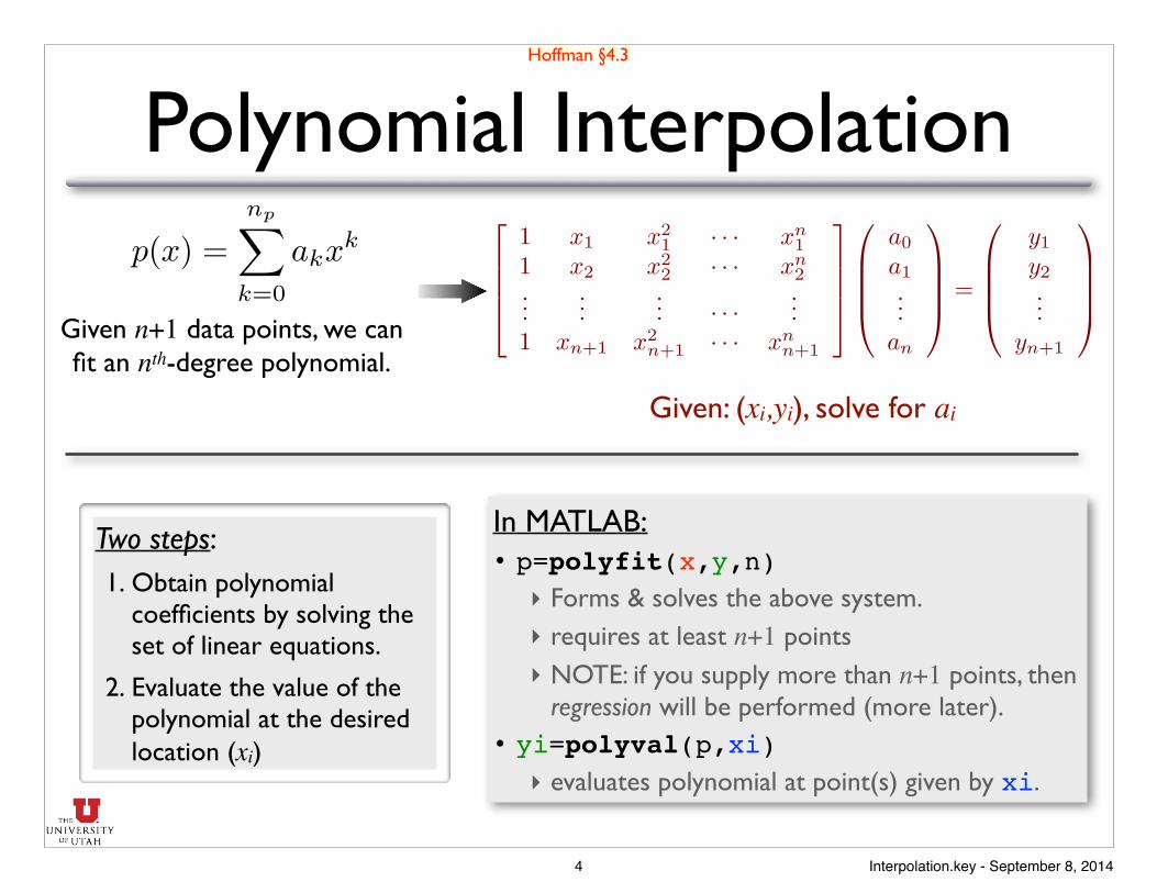
T rho lambda viscosity!K kg/m3 W/(m K) N s/m2!

----------------------------------------! 100 3.5562 0.0093 7.110e-06! 150 2.3364 0.0138 1.034e-05! 200 1.7458 0.0181 1.325e-05! 250 1.3947 0.0223 1.596e-05! 300 1.1614 0.0263 1.846e-05! 350 0.9950 0.0300 2.082e-05! 400 0.8711 0.0338 2.301e-05! 450 0.7750 0.0373 2.507e-05! 500 0.6864 0.0407 2.701e-05! 550 0.6329 0.0439 2.884e-05! 600 0.5804 0.0469 3.058e-05! 650 0.5356 0.0497 3.225e-05! 700 0.4975 0.0524 3.388e-05! 750 0.4643 0.0549 3.546e-05! 800 0.4354 0.0573 3.698e-05! 850 0.4097 0.0596 3.843e-05! 900 0.3868 0.0620 3.981e-05! 950 0.3666 0.0643 4.113e-05!1000 0.3482 0.0667 4.244e-05

Properties of air at atmospheric pressure

Incropera & DeWitt, Fundamentals of Heat and Mass Transfer, 4th ed.

What is the value of the viscosity at

T=412 K?

p(x) =np�

k=0

akxk

Can Apply Polynomial Interpolation “Globally” or “Locally”

Linear interpolation (n=1)

Polynomial interpolation, n=2Polynomial interpolation, n=3


(x1,y1)

(x2,y2)(x3,y3)

Cubic Spline Interpolation

f3(x) = a3x3 + b3x

2 + c3x + d3

1. At each data point, the values of adjacent splines must be the same. This applies to all interior points (where two functions meet) ⇒ 2(n-1) constraints.

2. At each point, the first derivatives of adjacent splines must be equal (applies to all interior points) ⇒ (n-1) constraints.

3. At each point, the second derivative of adjacent splines must be equal (applies to all interior points) ⇒ (n-1) constraints.

4. The first and last splines must pass through the first and last points, respectively ⇒ 2 constraints.

5. The curvature (d2f / dx2) must be specified at the end points ⇒ 2 constraints.

• d2f / dx2 = 0 ⇒ “natural spline”

4n constraints

f1(x) = a1x3 + b1x

2 + c1x + d1

For n+1 points, we form n splines. We must specify 4 variables per spline

⇒ we need 4n equations.

Concept: use cubic polynomial and “hook” them together over a wide range of data...

f2(x) = a2x3 + b2x

2 + c2x + d2

Hoffman §4.9


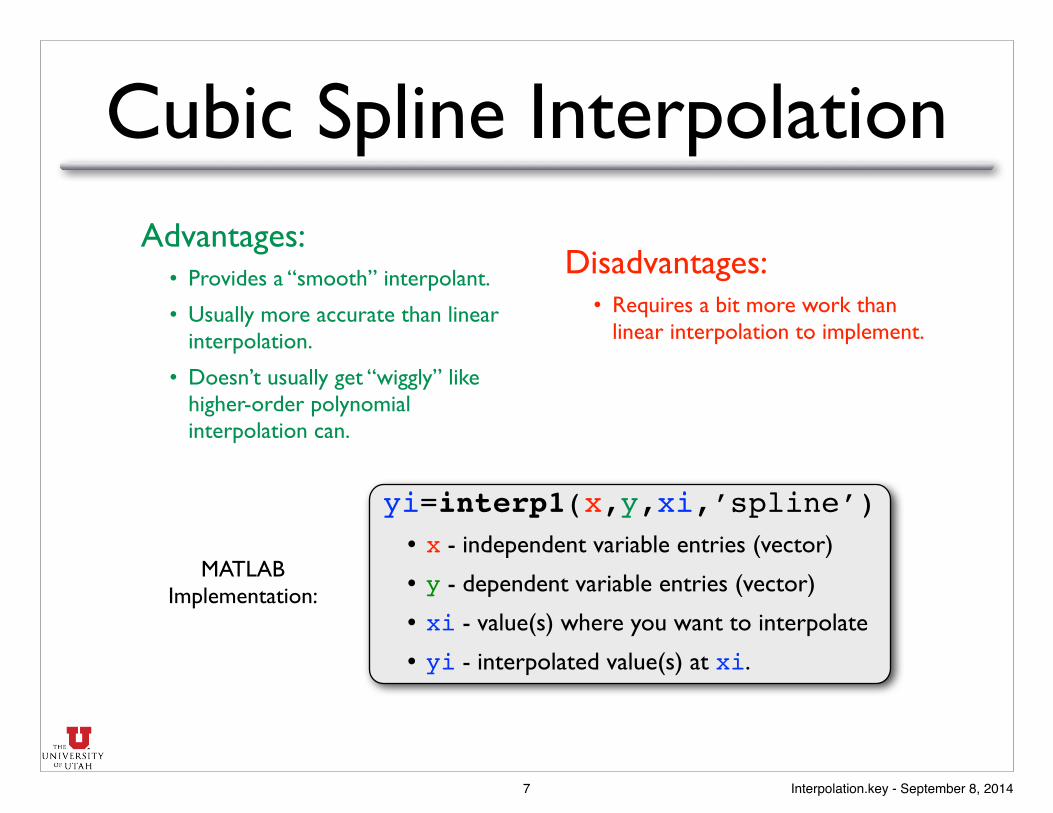
Cubic Spline InterpolationAdvantages:

• Provides a “smooth” interpolant.

• Usually more accurate than linear interpolation.

• Doesn’t usually get “wiggly” like higher-order polynomial interpolation can.

Disadvantages: • Requires a bit more work than

linear interpolation to implement.

yi=interp1(x,y,xi,’spline’) • x - independent variable entries (vector)

• y - dependent variable entries (vector)

• xi - value(s) where you want to interpolate

• yi - interpolated value(s) at xi.

MATLAB Implementation:


−1 −0.5 0 0.5 1

0.2

0.4

0.6

0.8

x

f(x)

f(x)Interpolating PointsPolynomialCubic SplineLinear

−1 −0.5 0 0.5 1

0.2

0.4

0.6

0.8

x

f(x)


Comparison Between Linear, Spline, & Polynomial Interpolation

f(x) = exp�� (x + b)2

c

⇥

Spline & polynomial are indistinguishable on this plot.

Increase number of data points.


−3 −2 −1 0 1 2 3−1

−0.5

0

0.5

1

x

f(x)

f(x)Interpolating PointsPolynomial, L2=2.6e+03Cubic Spline, L2=9.3e−01Linear, L2=7.9e−01

Polynomial interpolation can be bad if we use high-order polynomials

f(x) = tanh�x

a

⇥+ exp

⇤� (x + b)2

c

⌅Data points follow


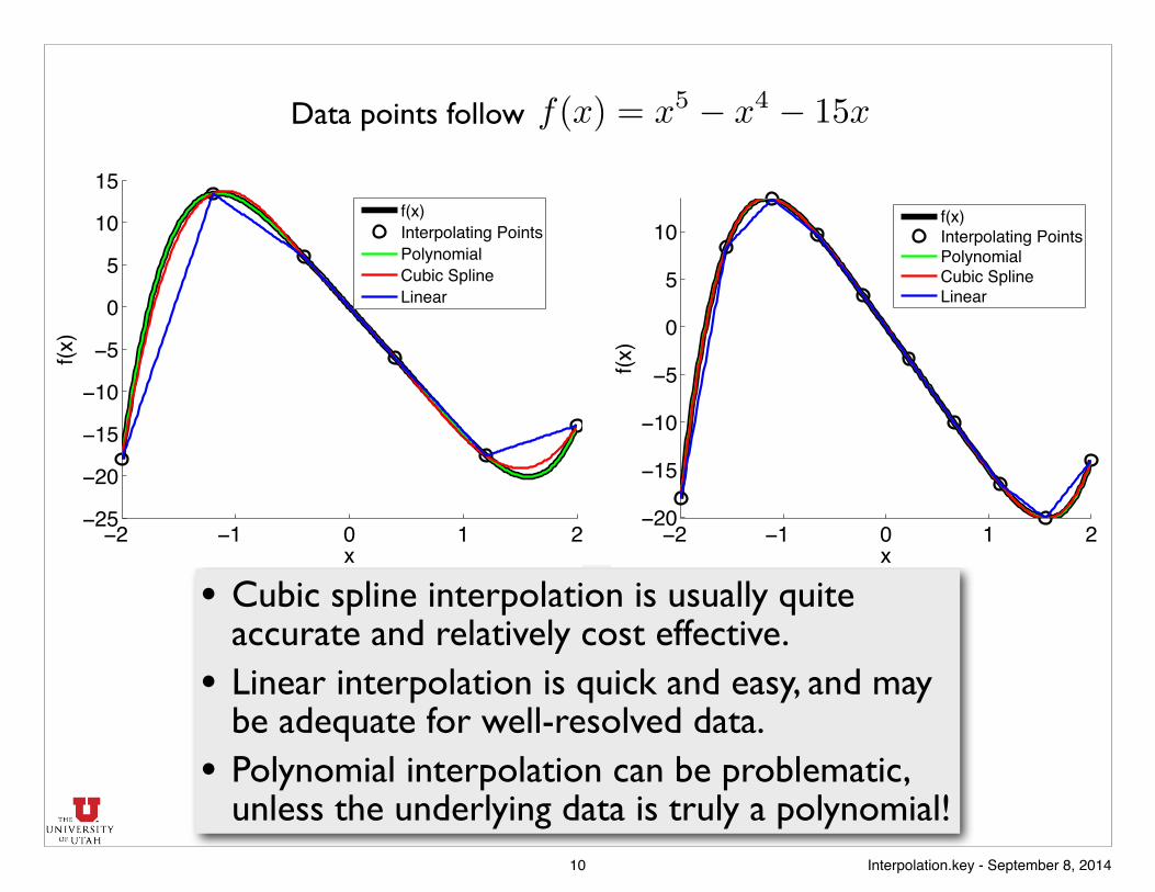
• Cubic spline interpolation is usually quite accurate and relatively cost effective.

• Linear interpolation is quick and easy, and may be adequate for well-resolved data.

• Polynomial interpolation can be problematic, unless the underlying data is truly a polynomial!

−2 −1 0 1 2−20

−15

−10

−5

0

5

10

x

f(x)


−2 −1 0 1 2−25

−20

−15

−10

−5

0

5

10

15

x

f(x)


f(x) = x5 � x4 � 15xData points follow


2-D Linear InterpolationIf you have “structured” (tabular) data:

1. Interpolate in one direction (two 1-D interpolations)

2. Interpolate in second direction.

Use this for simple homework assignments, in-class exams, etc.

ϕ=interp2(x,y,ϕ,xi,yi,’method’) • ‘linear’ - 2D linear interpolation (default) • ‘spline’ - 2D spline interpolation

Interpolate y firstInterpolate x first

�

�

x

y

x1

y1

x2

y2

�2,1

�2,2�1,2

�1,1

x

y

x1

y1

x2

y2

�2,1

�2,2�1,2

�1,1

Bilin

ear

inte

rpol

atio

n

x,y may be vectors (matlab assumes tabular form) ϕ must be a matrix (unique ϕ for each x-y pair)

Hoffman §4.8.1

�(x, y) ⇡ �1,1(x2 � x)(y2 � y)

(x2 � x1)(y2 � y1)

+ �2,1(x� x1)(y2 � y)

(x2 � x1)(y2 � y1)

+ �1,2(x2 � x)(y � y1)

(x2 � x1)(y2 � y1)

+ �2,2(x� x1)(y � y1)

(x2 � x1)(y2 � y1)


General 2-D Linear Interpolation� = ax + by + c

x

y�1 = ax1 + by1 + c

�2 = ax2 + by2 + c

�3 = ax3 + by3 + c

a =�3 (y1 � y2) + �2 (y3 � y1) + �1 (y2 � y3)x3 (y1 � y2) + x2 (y3 � y1) + x1 (y2 � y3)

,

b =�3 (x2 � x1) + �2 (x1 � x3) + �1 (x3 � x2)y3 (x2 � x1) + y2 (x1 � x3) + y1 (x3 � x2)

,

c =�3 (x1y2 � x2y1) + �2 (x3y1 � x1y3) + �1 (x2y3 � x3y2)

x1 (y2 � y3) + x2 (y3 � y1) + x3 (y1 � y2)

�1

�2

�3�

ϕ=interp2(x,y,ϕ,xi,yi,’method’) • ‘linear’ - linear interpolation

• ‘spline’ - spline interpolation

x, y, ϕ are matrices (unique x,y for each ϕ).

Data is NOT “structured”

Note: multidimensional higher-order interpolation methods exist (e.g. computer graphics industry)

Hoffman §4.8.2

Equation of a plane:

Solve 3 equations for 3 unknowns:


Documents

Interpolation - University of Utah - · PDF fileMATLAB Implementation: 7 Interpolation.key - September 8, 2014 −1 −0.5 0 0.5 1 0.2 0.4 0.6 0.8 x f(x) f(x) Interpolating Points