Internet-Based Teaching and Learning in Calculus Across All Dimensions

Thomas Banchoff

Brown University Thomas_Banchoff@brown.edu

New developments in visualization and communication software make it possible to present the calculus of functions of two variables in ways that reinforce topics in one-variable calculus while pointing forward to calculus in three and more variables. This paper surveys recent progress in this area with specific attention to the current course in Honors Multivariable Calculus taught by the author at Brown University, based on materials and programs developed over several years in collaboration with undergraduate student assistants. Highlighted examples include a geometric characterization of continuity, as well as explicit investigation of key examples involving the Intermediate Value Theorem and Clairaut’s Theorem on equality of mixed partial derivatives.

The author’s current course includes 66 students, all but two of them first-year students, many of them international students from China, Korea, India, and Thailand. With their permission, we will refer specifically to the work of two students from Thailand, Soravit Changpinyo and Thunwa Theerakarn, both of whom are graduates of Mahidol Wittayanusorn School, the first science school in Thailand.

In Soravit’s Mathematical Autobiography, written the first day of the course, he states: “There are three things I expect from this class. The first thing is challenging stuff. Math that’s too easy isn’t fun. Another thing is a strong foundation in calculus that will ease my learning in computer science. Lastly, I would like to learn about math not only from the instructors, but also from my peers. I know everyone is exceptionally talented.” He indicated in his questionnaire that my course had been recommended to him by Saran Ahuja, a member of the Thai Mathematical Olympiad team when he was a student at the Montford School in Chiangmai, and one of the top students in my course in Honors Linear Algebra during his first semester at Brown three years ago.

Thunwa writes “At the end of my high school years, I won a Thai Government scholarship to study in the United States from undergrad to Ph.D. The scholarship requires me to earn degree on Applied Mathematics and I will have to work in a university in Thailand for twice as time I will have spent here. This course will be hard - I know. Somebody told me I should not start first year in college with a hard course. But... there's so much to learn, and I'm willing to learn it. As always, it will be challenging, fun, and beautiful.”

Soravit’s comments refer to several features of this Internet-based course, including the procedure for submitting homework online and that fact that everyone in the class ultimately sees the work of all other students. Because the course is larger than usual, there has been more emphasis on group work this year, and students work together to a greater degree than previously. Groups are based in the various dormitories so it is easy for students to share ideas face to face as well as electronically.

Having students learn from one another is one of the best aspects of sharing documents on the Internet.

Other features of the course are contained in paragraphs written for a Brown University committee that selected this software for and award for teaching with technology:

Course Documentation is a file in the Resources menu that lists a number of tutorials, written by student assistants, giving shortcuts for entering mathematical symbols into typed responses that are treated as html code. A typical shortcut is x{^2} which prints as x2. The basic idea is that students don’t have to spend time learning a new computer language, and exponents and the square root sign, given by {sqrt} which prints as √, are the only mathematical typesetting they need for the first few assignments. After that, there is a more elaborate set of symbols that can be cut and pasted from a table. For students who want to upload their handwritten documents or pictures, there is an Upload Tutorial. There is also a tutorial on basic use of the Java applets that form the basis of the Laboratories for the course. For students who happen to know another system, like Mathematics, Maple, Mathcad, or The Geometer’s Sketchpad, or LaTeX, there are other tutorials, but from the beginning it is made clear that no exposure to these advanced systems is expected.

Interactive Laboratories: Under the Resources Menu in the course webpage, there is a link to the interactive laboratories developed using the senior thesis of David Eigen, a math-CS concentrator who devised the program for generating Java applets for use in a variety of mathematics courses at Brown. The Math 35 page includes a basic tutorial for using the Java demos. Each section of the labs starts with a labeled picture and a plus sign that can be selected to see more information about the concept illustrated in the demo. as well as a button that opens a Java applet. The student can explore a particular phenomenon, entering in new data and manipulating the images. In order to share what he or she has discovered or created, the student can save the applet tag and enter it into a homework answer or a discussion. Anyone who opens the button that appears in the document will enter the program exactly where the student left off. The instructor or another student can then make comments, sometimes illustrated by a modification of the given applet.

Each topic listed in the two-dimensional table of contents is in a column according to its dimension. At any time, a student can move “leftward” from a laboratory demonstration on two-variable calculus to the corresponding demonstration for one-variable calculus, or “rightward” to see how the notion will be extended to functions of three or more variables.

We illustrate this setup with two examples. The first involves continuity, a notion that many students understand only imperfectly after a first course in calculus, especially from a geometric point of view that can be particularly helpful in calculus of two variables. We interpret continuity as a challenge-response situation, and in any number of variables, the process is the same. Given a function f(x) of one variable and a point x0 of the domain, the challenger chooses a pair of horizontal lines at distance ε from y = f(x0) and asks if the domain can be restricted to points with distance less than δ from x0 so that the graph over that restricted domain lies between the two horizontal lines. If every challenge can be met, then the function is continuous at x0. In the case of a function of two variables, the challenge is the same, except that there are two horizontal planes at distance ε from the plane z = f(x0,y0) and the responder has to choose δ so small that the graph over the disc of radius δ centered at (x0,y0) lies between the planes.

[2 DEMOS]

Another example refers to the author’s paper in Volume 2, Number 2 of eJMT [B]. Critical points of a function of one variable can be visualized by coloring the graph of a function f(x) red if the derivative f’(x) is positive. Similarly critical points of a function of two variables can be visualized by coloring the graph of a function f(x,y) red if fx(x,y) is positive, blue if fy(x.y) is positive, and purple if both are positive.

[2 DEMOS]

Threaded Discussions: The Discussions menu item leads to a fairly standard sort of threaded discussion group moderated by the instructors. All students in all sections were able to participate in some open-ended questions, like the Height-Weight problem which was:

Was there a time since your birth when your height in inches was precisely equal to your weight in pounds?

Other discussions introduced new applets to go along with lectures and homework or provided additional hints for scanning.

Weekly Assignments: The Assignments menu gives the assignments for the course, in most cases along with a Solution Key developed each week. Solutions were largely compilations of answers submitted by students, often showing multiple approaches for solving the same problem. When an assignment is composed, it includes a time when it is open to the student, usually Thursday evening, and a time when the assignment is due, usually 3 a.m. on Monday morning. Up to that time only the student can see what he or she has submitted, and the comments of the instructor. After that time, everyone can see the responses of every other student in that section, together with comments, unless a student or the instructor has checked the box that designates a particular submission as "private". (Students routinely consider this sharing aspect of the software to be its most valuable feature.)

The Tensor: The Tensor is where all the responses are collected. By default only the last five assignments are presented in a matrix, and selecting "Show All Assignments" will present all the entries of all students over the course of the semester. Selecting a week or other heading in the leftmost column with open a matrix for that assignment, with problems listed on the leftmost column and student user id initials across the top. Selecting any entry shows the students response and the comment of the instructor. A square in the matrix is red if the most recent response came from the student and green if the most recent activity is a comment from the instructor. Mathematical autobiographies are automatically private, so they can only be read by the instructors for the class.

Students in this course meet for an hour and twenty minutes on Tuesdays and Thursdays. They hand in homework twice a week, a shorter assignment given after class on Tuesday, due by

Wednesday evening, and a longer assignment given after the Thursday class due by Monday morning at 3 a.m. Students receive responses for their work before the next class, so that by Monday evening there will be a Solution Key available online, primarily composed of interesting responses from students in the class, together with comments from me, or from my undergraduate assistant, Tan Van Nguyen, a third year student from Hanoi, Viet Nam, concentrating in Applied Mathematics/Economics, who helps to respond to the more standard questions in the assignments.

One (unintended) consequence of the ability to respond to comments is that some students engage in a dialogue until they get all the aspects of a problem correct. While this is certainly beneficial to the student, it involves extra time on the part of the instructor. Even without such back-and-forth online discussion, the practice of providing responses before the beginning of the next class involves a serious time commitment on the part of the instructor.

An illustration of this process came in the first assignment, where Thunwa typed in his answer to the following problem:

Problem: What is the range of the function f(x,y) = x2 + 2bxy + y2, defined for all (x,y)? (The answer will depend on b. Try to cover all possible cases.)

Thunwa Theerakarn at 2008-09-07 17:07:43.0

To find the range of the function f(x,y) = x2 + 2bxy + y2, for any y, we can choose t = x + by. Then f(x,y) = t2 + (1- b2) y2 Case |b| ≤ 1 : Since t2 ≥ 0 and (1- b2) y2 ≥ 0, we have f(x,y) ≥ 0. Range is all positive real numbers and zero. Case |b| < 1 : Since t2 can be any positive real number and (1- b2) y2 can be any negative real number, range of f(x,y) is all real numbers.

In the first assignment, students were required to type their answers using ordinary text together with simplified html shortcuts for exponents and the square root symbol. In the second assignment, students were required to include either a embedded link to and outside source or to an uploaded page, or a button for opening a Java applet using the visualization software demonstrated in class (and described in the Resources menu on the website).

Soravit’s entry for the second week includes material using the course software as well as other programs like Mathematics and Maple and MathCad, all available by site licenses at Brown. Here is his response to two of the problems assigned that week:

Problem: A function of one variable f(x) defined for all real x is said to have the Intermediate Value Property (IVP) if, for any a and b in the domain, if C is between f(a) and f(b), then there is a c between a and b such that f(c) = C.

a) Show that the function f(x) = sin(1/x) for x ≠ 0 and f(0) = 1/2 has the IVP (Note that this function is not continuous, so the IVP is not the same condition as continuity).

b) Find two functions f and g with the IVP so that f-g does not have the IVP, where (f-g)(x) is defined to be f(x) - g(x). (This is quite different from the situation for continuity, where the difference of two continuous functions will necessarily be continuous. We'll discuss this further in class.)

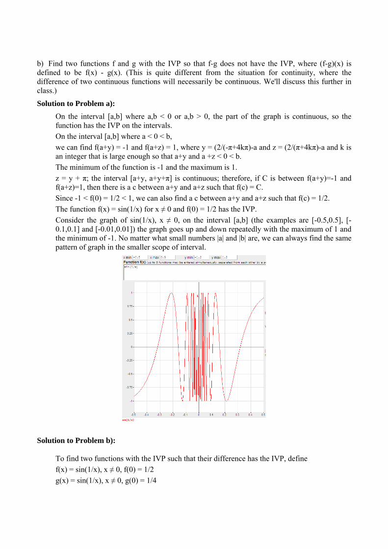
Solution to Problem a): On the interval [a,b] where a,b < 0 or a,b > 0, the part of the graph is continuous, so the function has the IVP on the intervals. On the interval [a,b] where a < 0 < b, we can find f(a+y) = -1 and f(a+z) = 1, where y = (2/(-π+4kπ)-a and z = (2/(π+4kπ)-a and k is an integer that is large enough so that a+y and a +z < 0 < b. The minimum of the function is -1 and the maximum is 1. z = y + π; the interval [a+y, a+y+π] is continuous; therefore, if C is between f(a+y)=-1 and f(a+z)=1, then there is a c between a+y and a+z such that f(c) = C. Since -1 < f(0) = 1/2 < 1, we can also find a c between a+y and a+z such that f(c) = 1/2. The function f(x) = sin(1/x) for x ≠ 0 and f(0) = 1/2 has the IVP. Consider the graph of sin(1/x), x ≠ 0, on the interval [a,b] (the examples are [-0.5,0.5], [-0.1,0.1] and [-0.01,0.01]) the graph goes up and down repeatedly with the maximum of 1 and the minimum of -1. No matter what small numbers |a| and |b| are, we can always find the same pattern of graph in the smaller scope of interval.

Solution to Problem b):

To find two functions with the IVP such that their difference has the IVP, define f(x) = sin(1/x), x ≠ 0, f(0) = 1/2 g(x) = sin(1/x), x ≠ 0, g(0) = 1/4

(Both are non-continuous functions with the IVP ; this makes it possible that the difference of them will not result in a continuous function that guarantees the IVP.) (f-g)(x) = 0, x ≠ 0, f(0) = 1/4. The difference function does not have the IVP. It is similar to the Dirac delta function, with f(x) = 0 for x ≠ 0 and f(0) = 1.

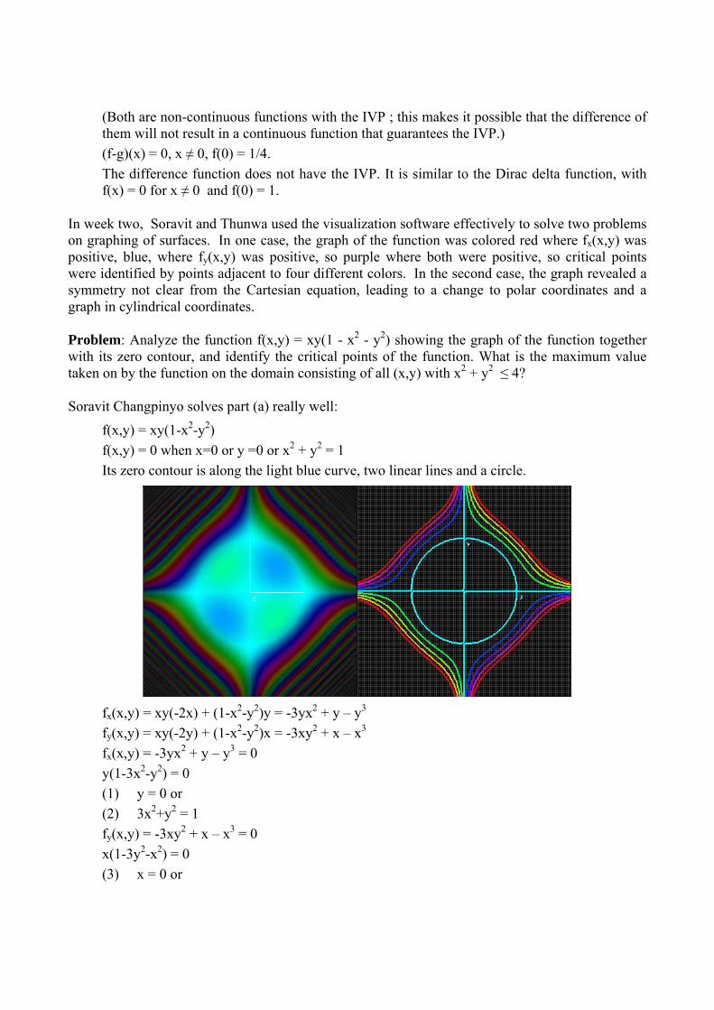
In week two, Soravit and Thunwa used the visualization software effectively to solve two problems on graphing of surfaces. In one case, the graph of the function was colored red where fx(x,y) was positive, blue, where fy(x,y) was positive, so purple where both were positive, so critical points were identified by points adjacent to four different colors. In the second case, the graph revealed a symmetry not clear from the Cartesian equation, leading to a change to polar coordinates and a graph in cylindrical coordinates.

Problem: Analyze the function f(x,y) = xy(1 - x2 - y2) showing the graph of the function together with its zero contour, and identify the critical points of the function. What is the maximum value taken on by the function on the domain consisting of all (x,y) with x2 + y2 ≤ 4?

Soravit Changpinyo solves part (a) really well:

f(x,y) = xy(1-x2-y2) f(x,y) = 0 when x=0 or y =0 or x2 + y2 = 1 Its zero contour is along the light blue curve, two linear lines and a circle.

fx(x,y) = xy(-2x) + (1-x2-y2)y = -3yx2 + y – y3 fy(x,y) = xy(-2y) + (1-x2-y2)x = -3xy2 + x – x3 fx(x,y) = -3yx2 + y – y3 = 0 y(1-3x2-y2) = 0 (1) y = 0 or (2) 3x2+y2 = 1 fy(x,y) = -3xy2 + x – x3 = 0 x(1-3y2-x2) = 0 (3) x = 0 or

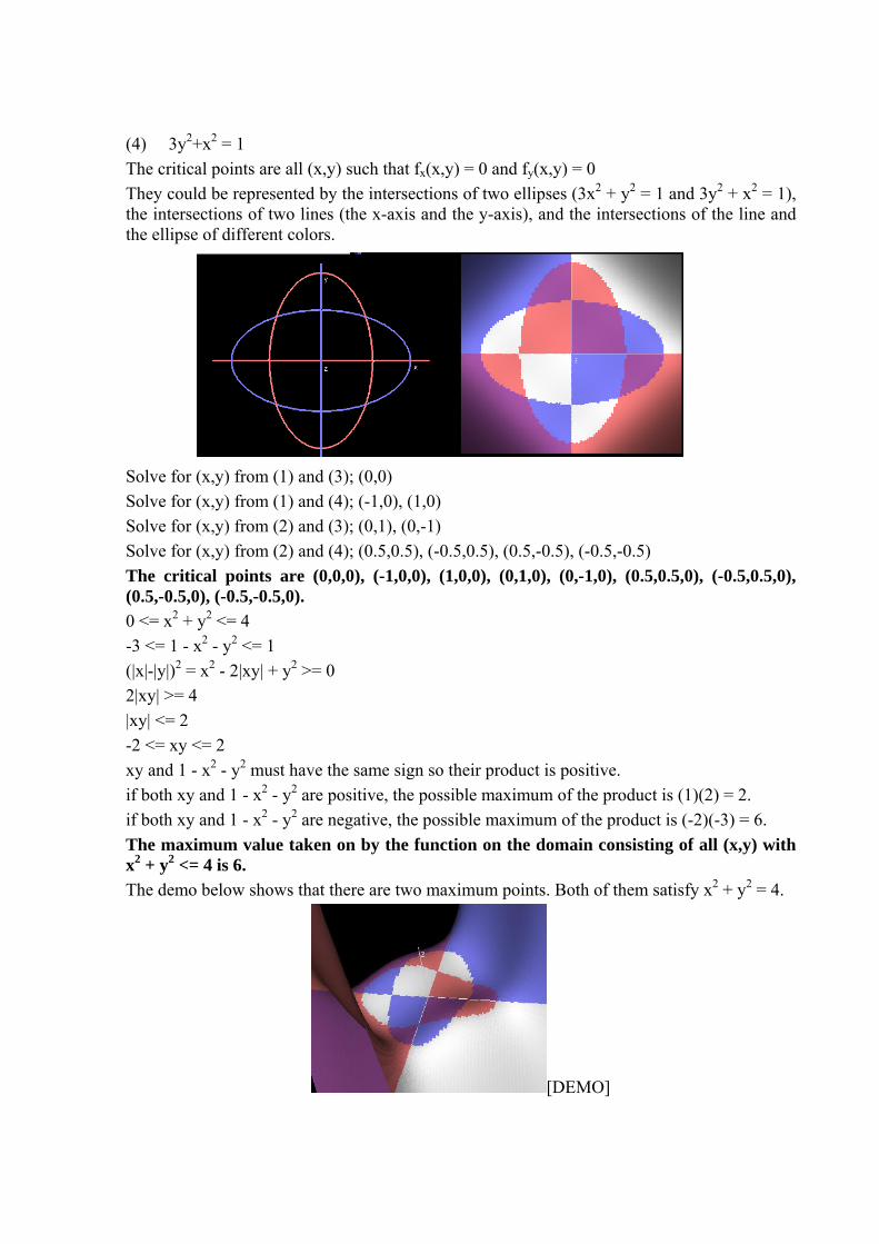
(4) 3y2+x2 = 1 The critical points are all (x,y) such that fx(x,y) = 0 and fy(x,y) = 0 They could be represented by the intersections of two ellipses (3x2 + y2 = 1 and 3y2 + x2 = 1), the intersections of two lines (the x-axis and the y-axis), and the intersections of the line and the ellipse of different colors.

Solve for (x,y) from (1) and (3); (0,0) Solve for (x,y) from (1) and (4); (-1,0), (1,0) Solve for (x,y) from (2) and (3); (0,1), (0,-1) Solve for (x,y) from (2) and (4); (0.5,0.5), (-0.5,0.5), (0.5,-0.5), (-0.5,-0.5) The critical points are (0,0,0), (-1,0,0), (1,0,0), (0,1,0), (0,-1,0), (0.5,0.5,0), (-0.5,0.5,0), (0.5,-0.5,0), (-0.5,-0.5,0). 0 <= x2 + y2 <= 4 -3 <= 1 - x2 - y2 <= 1 (|x|-|y|)2 = x2 - 2|xy| + y2 >= 0 2|xy| >= 4 |xy| <= 2 -2 <= xy <= 2 xy and 1 - x2 - y2 must have the same sign so their product is positive. if both xy and 1 - x2 - y2 are positive, the possible maximum of the product is (1)(2) = 2. if both xy and 1 - x2 - y2 are negative, the possible maximum of the product is (-2)(-3) = 6. The maximum value taken on by the function on the domain consisting of all (x,y) with x2 + y2 <= 4 is 6. The demo below shows that there are two maximum points. Both of them satisfy x2 + y2 = 4.

[DEMO]

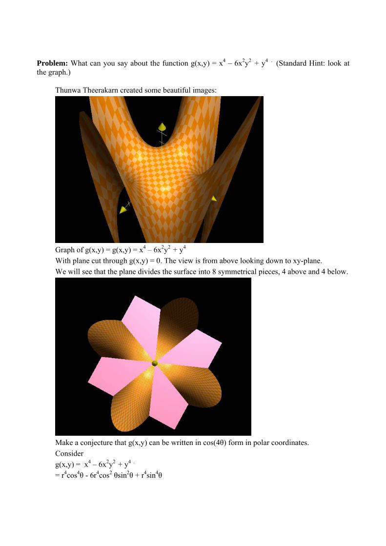
Problem: What can you say about the function g(x,y) = x4 – 6x2y2 + y4 . (Standard Hint: look at the graph.)

Thunwa Theerakarn created some beautiful images:

Graph of g(x,y) = g(x,y) = x4 – 6x2y2 + y4 With plane cut through g(x,y) = 0. The view is from above looking down to xy-plane. We will see that the plane divides the surface into 8 symmetrical pieces, 4 above and 4 below.

Make a conjecture that g(x,y) can be written in cos(4θ) form in polar coordinates. Consider g(x,y) = x4 – 6x2y2 + y4 . = r4cos4θ - 6r4cos2 θsin2θ + r4sin4θ

= [r4cos4θ - 2r4cos2θsin2θ + r4sin4θ] - 4r4cos2 θsin2θ = [r4[cos2θ -sin2θ]2] - r4sin2 (2θ) = r4[cos2 (2θ)2 - r4sin2 (2θ) = r4cos(4θ) Therefore, zero contour level is lines cos(4θ) = 0, that is, the lines θ = π/8 , 3π/8 , 5π/8 , 7π/8, 9π/8, 11π/8, 13π/8, 15π/8.

An example of Thunwa’s work from the assignment in the fourth week is:

Problem: Find the points of the ellipse x2 + xy + y2 = 1 closest to the origin and furthest from the origin by finding the critical points of f(x,y) = x2 + y2 on the ellipse. (See the Hint to recall the procedure for Lagrange multipliers.)

Solution to Problem:

Let g(x,y) = x2 + xy + y2 f(x,y) = x2 + y2 Consider the minimum and maximum of f(x,y) on level curve g(x,y) = 1 Using Lagrange multipliers, ∇ f(x,y) = λ∇ g(x,y) ∇ f(x,y) = (2x,2y) ∇ g(x,y) = (2x+y,2y+x) 2x = λ(2x+y) and 2y = λ(2y+x) That is 2x/(2x + y) = 2y/(2y + x) that is x2 = y2 Case x = y from g(x,y) we get that x2 + x(x) + x2 = 1 That is 3x2 = 1 x = 1/√3 (x,y) = (1/√3,1/√3) , (-1/√3,-1/√3) f(x,y) = x2 + y2 = 2/3 Case x = -y From g(x,y) = 1, we get that x2 = 1 That is x = ±1 (x,y) = (1,-1) , (-1,1) f(x,y) = x2 + y2 = 2 Therefore, g(x,y) closest to the origin at (x,y) = (1/√3,1/√3) , (-1/√3,-1/√3) and furthest at (x,y) = (1,-1) , (-1,1).

Problem: Find the critical points of the function f(x,y,z) = x2 + y2 + z2 on the ellipsoid x2 + y2/4+ z2/9 = 1 and indicate whether they are maxima or minima or other.

Here is a demo intended to give some inspiration. Changing r will alter the radius of an expanding sphere, representing the contour surfaces of f(x,y,z). What happens when the sphere and the ellipsoid intersect?

[DEMO]

Solution to Problem:

f(x,y,z) = x2 + y2 + z2 Let g(x,y,z) = x2 + y2/4 + x2/9 Consider the critical points of f(x,y,z) on the level set of g(x,y,z) = 1 Using Lagrange multipliers ∇ f(x,y,z) = λ∇ g(x,y,z) That is (2x+2y+2z) = λ(2x+y/2+2z/9) implies 2x = λ2x 2y = λy/2 2z = λ2z/9 That is x = 0 or λ = 1 y = 0 or λ = 4 z = 0 or λ = 9 Consider that in each case, λ cannot be the same constant. Therefore, two of {x,y,z} have to equal zero in each case. When x=0, z=0, y=±2 f(x,y,z) = 4 When x=0,y=0 , z=±3 f(x,y,z) = 9

When y=0, z=0 , x=±1 f(x,y,z) = 1 Therefore, (0,0,±3) are maxima, (±1,0,0) are minima and (0,±2,0) are critical points but not maxima or minima. At the critical points, the gradient vectors of f and g are parallel

Critical Points at Level f(x,y,z) = 2

The Midterm Examination

We take our final illustration from one of the problems on the midterm examination. The first examination in the course took place four weeks after the start of the semester. The Midterm Examination was a take-home test over a period of six days. It consisted of ten problems, each with two or three parts, and students were permitted to use notes and books and computers, as well as all the material on the class website, but they all agreed that no one would consult anyone else, either in person or electronically.

The first problem required students to identify the critical points of a polynomial function f(x,y) = x4 – 2x2 – y2 and to find the maximum and minimum values on a disc of radius R centered at the origin, where the result depended on R.

The last part of the problem was subtle enough to test the ingenuity of most students. William Fallon devised a demonstration that was particularly useful in seeing how the image of a disk of radius R changed with R,

Gili Kriger was able to construct a two-dimensional graphic showing five different functions of R on the same diagram, from which it was possible to read off the required maxima and minima, and to provide algebraic justification for the listing of results.

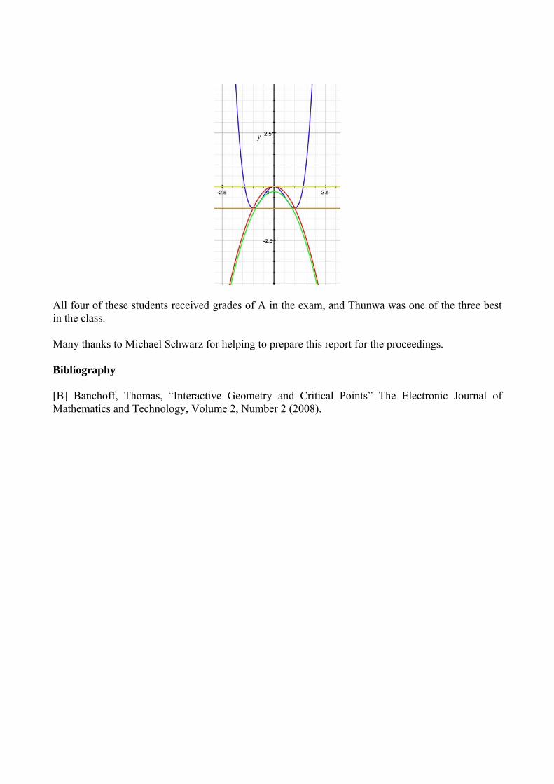
All four of these students received grades of A in the exam, and Thunwa was one of the three best in the class.

Many thanks to Michael Schwarz for helping to prepare this report for the proceedings.

Bibliography

[B] Banchoff, Thomas, “Interactive Geometry and Critical Points” The Electronic Journal of Mathematics and Technology, Volume 2, Number 2 (2008).