International Workshop - arxiv.org · 6 Victor P. Maslov It was was impossible at the time to implement this e ect in practice, which would have allowed to obtain a unimode laser,

Independent University of MoscowFrench–Russian Laboratory “J.-V. Poncelet”

International Workshop

IDEMPOTENT AND TROPICAL MATHEMATICSAND PROBLEMS OF MATHEMATICAL PHYSICS

G.L. Litvinov, V.P. Maslov, S.N. Sergeev (Eds.)

Organizing committee: G.L. Litvinov, V.P. Maslov,S.N. Sergeev, A.N. Sobolevskiı

Web-site: http://www.mccme.ru/tropical07

E-mail: [email protected]

Moscow, August 25–30, 2007

Volume II

Moscow, 2007

arX

iv:0

709.

4119

v1 [

mat

h.R

A]

26

Sep

2007

Litvinov G.L., Maslov V.P., Sergeev S.N. (Eds.)Idempotent and tropical mathematics and problems ofmathematical physics (Vol. II) – M.: 2007 – 116 pages

This volume contains the proceedings of an InternationalWorkshop on Idempotent and Tropical Mathematics andProblems of Mathematical Physics, held at the IndependentUniversity of Moscow, Russia, on August 25-30, 2007.

2000 Mathematics Subject Classification: 00B10,81Q20, 06F07, 35Q99, 49L90, 46S99, 81S99, 52B20,52A41, 14P99

c© 2007 by the Independent University of Moscow. All rights reserved.

CONTENTS

Ultrasecond quantization of a classical version ofsuperfluidity in nanotubes

Victor P. Maslov . . . . . . . . . . . . . . . . . . . . . . . . . . . . . . . . . . . . . . . . . . . . . . . . . . . . . .5

Policy iteration and max-plus finite element method

David McCaffrey . . . . . . . . . . . . . . . . . . . . . . . . . . . . . . . . . . . . . . . . . . . . . . . . . . . . . 11

Using max-plus convolution to obtain fundamental solutionsfor differential equations with quadratic nonlinearities

William M. McEneaney . . . . . . . . . . . . . . . . . . . . . . . . . . . . . . . . . . . . . . . . . . . . . . 21

Polynomial quantization on para-hermitian symmetric spacesfrom the viewpoint of overgroups: an example

Vladimir F. Molchanov . . . . . . . . . . . . . . . . . . . . . . . . . . . . . . . . . . . . . . . . . . . . . . 30

The structure of max-plus hyperplanes

V. Nitica and I. Singer . . . . . . . . . . . . . . . . . . . . . . . . . . . . . . . . . . . . . . . . . . . . . . 37

Image processing based on a partial differential equation sat-isfying the pseudo-linear superposition principle

E. Pap and M. Strboja . . . . . . . . . . . . . . . . . . . . . . . . . . . . . . . . . . . . . . . . . . . . . . . 38

Tropical analysis on plurisubharmonic singularities

Alexander Rashkovskii . . . . . . . . . . . . . . . . . . . . . . . . . . . . . . . . . . . . . . . . . . . . . . . 43

Minimal elements and cellular closures over the max-plussemiring

Sergeı Sergeev . . . . . . . . . . . . . . . . . . . . . . . . . . . . . . . . . . . . . . . . . . . . . . . . . . . . . . . .49

Semiclassical quantization of field theories

Oleg Yu. Shvedov . . . . . . . . . . . . . . . . . . . . . . . . . . . . . . . . . . . . . . . . . . . . . . . . . . . . 52

Convex analysis, transportation and reconstruction of pecu-liar velocities of galaxies

Andreı Sobolevskiı . . . . . . . . . . . . . . . . . . . . . . . . . . . . . . . . . . . . . . . . . . . . . . . . . . . .57

The Weyl algebra and quantization of fields

Alexander V. Stoyanovsky . . . . . . . . . . . . . . . . . . . . . . . . . . . . . . . . . . . . . . . . . . . .58

Polynomial quantization on para-hermitian spaces withpseudo-orthogonal group of translations

Svetlana V. Tsykina . . . . . . . . . . . . . . . . . . . . . . . . . . . . . . . . . . . . . . . . . . . . . . . . . 63

The horofunction boundary

Cormac Walsh . . . . . . . . . . . . . . . . . . . . . . . . . . . . . . . . . . . . . . . . . . . . . . . . . . . . . . . 71

Quantization as approximate description of a diffusion process

(in Russian)

Evgeny M. Beniaminov . . . . . . . . . . . . . . . . . . . . . . . . . . . . . . . . . . . . . . . . . . . . . . 78

Idempotent systems of nonlinear equations and computational

problems arising in electroenergetic networks (in Russian)

A.M. Gel’fand and B.Kh. Kirshteyn . . . . . . . . . . . . . . . . . . . . . . . . . . . . . . . . . .84

Classical and nonarchimedean amoebas in extensions of fields

(in Russian)

Oksana V. Znamenskaya . . . . . . . . . . . . . . . . . . . . . . . . . . . . . . . . . . . . . . . . . . . . . 88

Generalization of ultra second quantization for fermions at

non-zero temperature (in Russian)

G.V. Koval and V.P. Maslov . . . . . . . . . . . . . . . . . . . . . . . . . . . . . . . . . . . . . . . . .92

Contact classification of Monge-Ampere equations

(in Russian)

Alexey G. Kushner . . . . . . . . . . . . . . . . . . . . . . . . . . . . . . . . . . . . . . . . . . . . . . . . . . .99

On amoeba of discriminant of algebraic equation (in Russian)

Evgeny N. Mikhalkin . . . . . . . . . . . . . . . . . . . . . . . . . . . . . . . . . . . . . . . . . . . . . . . .104

Universal algorithms solving discrete Bellman systems of

equations over semirings (a computer demonstration)

(in Russian)

A.V. Chourkin and S.N. Sergeev . . . . . . . . . . . . . . . . . . . . . . . . . . . . . . . . . . . 107

The curves in C2 whose amoebas determine the fundamental

group of complement (in Russian)

Roman Ulvert . . . . . . . . . . . . . . . . . . . . . . . . . . . . . . . . . . . . . . . . . . . . . . . . . . . . . . .110

List of participants and authors. . . . . . . . . . . . . . . . . . . . . . . . . . . .112

Ultrasecond quantization 5

Ultrasecond quantization of a classical version ofsuperfluidity in nanotubes1

Victor P. Maslov

1. In order to distinguish the classical theory in its modern under-standing from the quantum theory, it is necessary to modify (somewhat)the ideology habitual to physicists, for whom the classical theory is sim-ply the whole body of physics as it existed in the 19th century before theappearance of quantum theory. Actually, the correct meaning is that theclassical theory is the limit of the quantum one as h→ 0.

Thus, Feynman correctly understood that spin is a notion of classicalmechanics. Indeed, it is obtained via a rigorous passage from quantummechanics to classical mechanics [1]. In a similar same way, the polariza-tion of light does not disappear when the frequency is increased, and istherefore a property of geometric rather than wave optics, contrary to thegenerally accepted belief, which arose because the polarization of light wasdiscovered as the result of the appearance of wave optics.

Consider a “Lifshits hole”, i.e. a one-dimensional Schrodinger equationwith potential symmetric with respect to the origin of coordinates with twotroughs. Its eigenfunctions are symmetric or antisymmetric with respectto the origin. As h → 0 this symmetry remains, and since the squareof the modulus of the eigenfunction corresponds to the probability of theparticle to remain in the troughs, it follows that in the limit as h→ 0, i.e.,in the “classical theory”, for energies less than those required to pass overthe barrier, the particle is simultaneously located in two troughs, althougha classical particle cannot pass through the barrier. Nevertheless, thissimple example shows how the ideology of the “classical theory” must bemodified.

To understand this paradox, one must take into consideration the factthat the symmetry must be very precise, up to “atomic precision”, andthat stationary state means a state that arises in the limit for “infinitelylong” time.

When we deal with nanotubes whose width is characterized by “atomic”or “quantum” dimensions, then new unexpected effects occur in the “clas-sical” theory. Thus, already in 1958 [2], I discovered a strange effect of thestanding longitudinal wave type in a slightly bent infinite narrow tube, forthe case in which its radius is the same everywhere with atomic precision.

1The work has been supported by the joint RFBR/CNRS grant 05-01-02807 and

by the RFBR grant 05-01-00824.

6 Victor P. Maslov

It was was impossible at the time to implement this effect in practice, whichwould have allowed to obtain a unimode laser, despite A.M.Prokhorov’sgreat interest in the effect.

2. Now let us discuss the notion known as “collective oscillations” inclassical physics and as “quasiparticles” in quantum physics. In classicalphysics, it is described by the Vlasov equation for selfcompatible (or mean)fields, in quantum physics, by the Hartrey (or the Hartrey-Fock) equation.

(1) Variational equations depend on where (i.e., near what solutions ofthe original equation) we consider the variations. For example, in [3, 4, 5]we considered variations near a microcanonical distribution in an ergodicconstruction, while in [7, 8, 9, 10] this was done near a nanocanonicaldistribution concentrated on an invariant manifold of lesser dimension, i.e.,not on a manifold of constant energy but, for example, on a Lagrangianmanifold of dimension coinciding with that of the configuration space.

(2) Let us note the following crucial circumstance. The solution ofthe variational equation for the Vlasov equation does not coincide withthe classical limit for variational equations for the mean field equations inquantum theory.

Consider the mean field equation in the form

ih∂

∂tϕt(x) =

(− h2

2m∆ +Wt(x)

)ϕt(x),

Wt(x) = U(x) +∫V (x, y)|ϕt(y)|2dy,

(1)

with the initial condition ϕ|t=0 = ϕ0, where ϕ0 belongs to W∞2 (Rν) andsatisfies

∫dx|ϕ0(x)|2 = 1.

In order to obtain asymptotics of the complex germ type [11] one mustwrite out the system consisting of the Hartrey equation and its dual, thenconsider the corresponding variational equation, and, finally, replace thevariations δϕ and δϕ∗ by the independent functions F and G. For thefunctions F and G, we obtain the following system of equations:

i∂F t(x)∂t

=∫dy

(δ2H

δϕ∗(x)δϕ(y)F t(y) +

δ2H

δϕ∗(x)δ∗ϕ(y)Gt(y)

);

− i∂Gt(x)∂t

=∫dy

(δ2H

δϕ(x)δϕ(y)F t(y) +

δ2H

δϕ(x)δ∗ϕ(y)Gt(y)

).

(2)

The classical equations are obtained from the quantum ones, roughlyspeaking, by means of a substitution of the form ϕ = χe

ihS (the VKB


method), ϕ∗ = χ∗eihS∗, where S = S∗, χ = χ(x, t) ∈ C∞, S = S(x, t) ∈

C∞.To obtain the variational equations, it is natural to take the variation

not only of the limit equation for χ and χ∗, but also for the functions Sand S∗. This yields a new important term of the equation for collectiveoscillations.

Let us describe this fact for the simplest example, which was studied inN.N.Bogolyubov’s famous paper concerning “weakly ideal Bose gas” [12].

Suppose U = 0 in equation (1) in a three-dimensional cubical box ofedge L, the wave functions satisfying the periodicity condition (i.e., theproblem being defined on the 3-torus with generators of lengths L,L,L).Then the function

(3) ϕ(x) = L−3/2ei/h(px−Ωt),

where p = 2πn/L, n is an integer, satisfies the equation (1) for

(4) Ω =p2

2m+ L−3

∫dxV (x).

For λ = 2πn/L, n a nonzero integer, consider the functions F (λ)(x)and G(λ)(x) given by

F (λ)t(x) = L−3/2ρλeih |(p+λ)x+(β−Ω)t|,

G(λ)t(x) = L−3/2σλeih |(−p+λ)x+(β+Ω)t|;

(5)

here

− βλρλ =(

(p+ λ)2

2m− p2

2m+ Vλ

)ρλ + Vλσλ,

βλρλ =(

(p− λ)2

2m− p2

2m+ Vλ

)σλ + Vλρλ,

|σλ|2 − |ρλ|2 = 1, Vλ = L−3

∫dxV (x)e

ihλx.

(6)

From the system (6), we find

(7) βλ = −pλ+

√(λ2

2m+ Vλ

)2

− V 2λ .

In this example u = eih s(x,t), u∗ = e−

s(x,t)h , where s(x, t) = px + βt,

while the variation of the action for the vector(δu, δu∗

)equals λx± Ωt.

8 Victor P. Maslov

Under a more accurate passage to the limit, we obtain

Vλ → V0 = L−3

∫dxV (x)

.Thus, in the classical limit, we have obtained the famous Bogolyubov

relation (7). In the case under consideration u(x) = 0 and, as in thelinear Schrodinger equation, the exact solution coincides with the quasi-classical one. In the paper [10], the case u(x) 6= 0 is investigated, and itturns out that the relation similar to (7) is the classical limit as h → 0of the variational equation in this general case. The curve showing thedependence of βλ on λ is known as the Landau curve and determines thesuperfluid state. The value λcr for which superfluidity disappears is calledthe Landau critical level. Bogolyubov explains the superfluidity phenome-non in the following terms: “the ‘degenerate condensate’ can move withoutfriction relatively to elementary perturbations with any sufficiently smallvelocity” [10, p. 210].

However, there is no Bose-Einstein condensate whatever in these math-ematical considerations, it is just that the spectrum defined for λ < λcr

is a positive spectrum of quasiparticles. This means it is metastable (see[13]). The Bose-Einstein condensate is not involved here, it is only neededonly to show that it would be wrong to believe that this argument worksfor a classical liquid, as one might think from the considerations above.

Indeed, for example, the molecules of a classical nondischarged liquidare, as a rule, Bose particles. For such a liquid, one can write out the N -particle equation, having in mind that each particle (molecule) is neutraland consists of an even number l of neutrons. Thus each ith particle is apoint in 3(2k + l)-dimensional space, where k is the number of electrons,xi ∈ R6k+3l, depends on the potential u(xi), xi ∈ R6k+3l and we can con-sider the N -particle equation for xi, i = 1, . . . , N , with pairwise interactionV (xi − xj).

3. However, there is a purely mathematical explanation of this para-dox. The thing is that Bogolyubov found only one series of points in thespectrum of the many particle problem. Landau wrote “N.N.Bogolyubovrecently succeeded, by means of a clever application of second quantiza-tion, in finding the general form of the energy spectrum of a Bose-Einsteingas with weak interaction between the particles” ([14, p. 43]). But thisseries is not unique, i.e., the entire energy spectrum was not obtained.

In 2001, the author proposed the method of ultra second quantization[15]; see also [16], [17], [18], [19], [20], The ultra second quantization ofthe Schrodinger equation, as well as its ordinary second quantization, is


a representation of the N -particle Schrodinger equation, and this meansthat basically the ultra second quantization of the equation is the same asthe original N -particle equation: they coincide in 3N -dimensional space.However, the replacement of the creation and annihilation operators by c-numbers, in contrast with the case of second quantization, does not yieldthe correct asymptotics, but it turns out that it coincides with the result ofapplying the Schroeder variational principle or the Bogolyubov variationalmethod.

For the exotic Bardin potential, the correct asymptotic solution co-incides with the one obtained by applying the ultra second quantizationmethod described above. In the case of general potentials, in particularfor pairwise interaction potentials, the answer is not the same. Specifi-cally, the ultra second quantization method gives other asymptotic seriesof eigenvalues corresponding to the N -particle Schrodinger equation, andthese eigenvalues, unlike the Bogolyubov ones (7), are not metastable.

It turns out that the main point is not related to the Bose-Einsteincondensate, but has to do with the width of the capillary (the nanotube)through which the liquid flows. If we consider a liquid in a capillaryor a nanotube of sufficiently small radius the velocity corresponding tometastable states is not small. Hence at smaller velocities the flow will bewithout friction.

The condition that the liquid does not flow through the boundary ofthe nanotube is a Dirichlet condition. It yields a standing wave, whichcan be regarded as a pair particle–antiparticle: a particle with momen-tum p orthogonal to the boundary of the tube, and an antiparticle withmomentum −p.

We consider a short action pairwise potential V (xi − xj). This meansthat as the number of particles tends to infinity, N → ∞, interaction ispossible for only a finite number of particles. Therefore, the potentialdepends on N in the following way:

VN = V ((xi − xj)N1/3).

If V (y) is finite with support ΩV , then as N → ∞ the support engulfs afinite number of particles, and this number does not depend on N .

As the result, it turns out that for velocities less than min(λcr,h

2mR ),where λcr is the critical Landau velocity and R is the radius of the nan-otube, superfluidity occurs.

Now let me present my own considerations, which are not related tothe mathematical exposition. Viscosity is due to the collision of particles:the higher the temperature, the greater the number of collisions. In a

10 Victor P. Maslov

nanotube, there are few collisions, and only with the walls, and those aretaken into account by the author’s series. It is precisely this circumstance,and not the Bose-Einstein condensate, which leads to the weakening ofviscosity and so to superfluidity. What I am saying is that the mainfactor in the superfluidity phenomenon, even for liquid helium 4, is notthe condensate, but the presence of an extremely thin capillary [21], [22].It seems to me that a neutral gas like argon could be used for a crucialexperiment.

Bibliography

[1] V. P. Maslov, Perturbation Theory and Asymptotic Methods. Nauka, Moscow, 1978(in Russian).

[2] V. P. Maslov, Doklady AN SSSR ,1958, 123(4), 631–633 (in Russian).

[3] V. P. Maslov, Quasi-Particles Associated with Lagrangian Manifolds and (in theErgodic Case) with Constant Energy Manifolds Corresponding to Semiclassical

Self- Consistent Fields. V. Russian J. Math. Phys., 1996, 3 (4), 529-534.

[4] V. P. Maslov. Russian J. Math. Phys., 1996, 4(1), 117-122[5] V. P. Maslov. Russian J. Math. Phys., 1996, 4(2), 266-270

[6] V. P. Maslov, A. S. Mishchenko, Quasi-classical asymptotics of quasi-particles.

Sbornik: Mathematics, 1998, 189(6), 901–930.[7] V. P. Maslov. Russian J. Math. Phys., 1995, 2(4), 527-534.

[8] V. P. Maslov. Russian J. Math. Phys., 1995, 3(1), 123-132.[9] V. P. Maslov. Russian J. Math. Phys., 1995, 3(2), 271-276.

[10] V. P. Maslov. Russian J. Math. Phys., 1995, 3(3), 401-406.

[11] V. P. Maslov, The Complex-VKB Method for Nonlinear Equations. Moscow,Nauka, 1977 (in Russian).

[12] N. N. Bogolyubov, On the theory of superfluidity. – In: Selected Works of N.N. Bo-

goliubov, Kiev, Naukova dumka, 1970, vol. 2, pages 210–224 (in Russian).[13] V. P. Maslov, O. Yu. Shvedov, The Complex Germ Method for Multiparticle and

Quantum Field Theory Problems, Moscow, Editorial URSS, 2000 (in Russian).

[14] L. D. Landau, On the theory of superfluidity.– In: Collected Papers of L.D. Landau,Moscow, Nauka, 1969, vol.2, pages 42–46 (in Russian). See also: Phys Rev., 75,884, 1949.

[15] V. P. Maslov, Quantization of Thermodynamics and Ultrasecond Quantization.Moscow, Institute of Computer Sciences, 2001 (in Russian).

[16] V. P. Maslov, Generalization of the Second Quantization Method to the Case of

Special Tensor Products of Fock Spaces and Quantization of Free Energy. Func-tional Analysis and Its Applications, Oct. 2000, 34(4), 265–275.

[17] V. P. Maslov, Super-second quantisation and entropy quantisation with chargeconservation. Russian Math. Surveys, 2000, 55 (6), 1157-1158.

[18] V. P. Maslov, Some Identities for Ultrasecond-Quantized Operators. Russian J.

Math. Phys., 2001, 8(3), 309-321.[19] V. P. Maslov, Quantization of Thermodynamics, Ultrasecondary Quantization and

a New Variational Principle. Russian J. Math. Phys., 2001, 8(1), 55–82

Policy Iteration & Max-Plus FEM 11

[20] V. P. Maslov, Ultratertiary quantization of thermodynamics. Theor. and Math.

Phys., 2002, 132(3), 1222–1232.

[21] V. P. Maslov, Dependence of the Superfluidity Criterion on the Capillary Radus.Theor. and Math. Phys., 2005, 143(3), 741–759.

[22] V. P. Maslov, Resonance between One-Particle (Bogoliubov) and Two-Particle

Series in a Superfluid Liquid in a Capillary. Russian J. Math. Phys., 2005, 12(3),369–379

Policy iteration and max-plus finite element method

David McCaffrey

1. Introduction

We consider the finite horizon differential game

(1.1) v(x, T ) = infa(.)

supb(.)

∫ T

0

12x(s)2 +

12a(s)2 − γ2

2b(s)2

ds+ φ(x(T ))

over trajectories (x(.), a(.), b(.)) satisfying x(s) = f(x(s)) + g(x(s))a(s) +h(x(s))b(s), x(0) = x, where x(s) ∈ X ⊆ Rn, a(s) ∈ U ⊆ Rm, b(s) ∈W ⊆ Rr.This problem arises, for example, as the differential game formu-lation of a well-known class of non-linear affine H∞ control problems - see[5, 6, 7, 4] for details. In particular it is known that the value functionv(x, t) for the finite horizon problem is a (possibly non-smooth) solutionto the Hamilton-Jacobi-Isaacs equation

(1.2) H(x, ∂v/∂x) = ∂v/∂t

with initial condition v(x, 0) = φ(x) for (x, t) ∈ X × (0, T ], where theHamiltonian is defined as

H(x, p) = mina

maxb

p (f(x) + g(x)a+ h(x)b) +

12x2 +

12a2 − γ2

2b2.

Note this Hamiltonian is non-convex in p.Suppose we choose some feedback function a(x) and, on any solution

trajectory (x(.), a(.), b(.)), define the control input a(s) = a(x(s)) for alls. We can then define fa(x, b) = f(x) + g(x)a(x) + h(x)b and la(x, b) =12x

2+ 12 a(x)2−γ

2

2 b2, and consider the finite horizon optimal control problem

(1.3) va(x, T ) = supb(.)

∫ T

0

la(x(s), b(s))ds+ φ(x(T ))

12 David McCaffrey

over trajectories (x(.), b(.)) satisfying x(s) = fa(x(s), b(s)), x(0) = x. Inthis case, the value function va(x, t) satisfies the Hamilton-Jacobi equation

(1.4) Ha(x, ∂va/∂x) = ∂va/∂t

with initial condition va(x, 0) = φ(x) for (x, t) ∈ X × (0, T ], where theHamiltonian is defined as Ha(x, p) = maxb pfa(x, b) + la(x, b) . Note thatthis Hamiltonian is convex in p for all x.

A max-plus analogue of the finite element method (FEM) is set outin [1] for the numerical computation of the value function va solving thisconvex optimal control problem (1.3). In this note, we set out a policyiteration algorithm for the solution of the non-convex differential game(1.1). This involves the use of the max-plus FEM to solve (1.4) for agiven fixed control feedback a(x) in the value determination step of thealgorithm, and then a QP to improve the control feedback in the policyimprovement step.We show here that the algorithm converges. It can alsobe shown that the approximation error on the converged solution is oforder

√∆t + ∆x(∆t)−1, the same order as that obtained in [1] for the

errors associated with the max-plus FEM. We do not give details of thisresult here, due to limited space.

2. The Max-Plus Finite Element Method

In the following, let St denote the evolution semi-group of the PDE (1.2).This associates to any function φ, the function vt = v(., t) where v is thevalue function of the differential game (1.1). Similarly, let Sta denote theevolution semi-group of the PDE (1.4) for some fixed feedback functiona(.). This associates to any function φ, the function vta = va(., t) whereva is the value function of the otimal control problem (1.3). Maslov [3]observed that the semi-group Sta is max-plus linear. We now briefly reviewthe max-plus finite element method (FEM) set out in [1] for the numericalcomputation of va

Let Rmax denote the idempotent semi-ring obtained from R, with itsusual order ≤, by defining idempotent addition as a⊕ b := max(a, b) andmultiplication as ab := a + b. Then let Rmax := Rmax ∪ +∞, with theconvention that −∞ is absorbing for the mutiplication.

For X a set, we consider the set RXmax of Rmax valued functions on X.This is a semimodule over Rmax with respect to componentwise addition(u, v) 7−→ u⊕ v, defined by (u⊕ v)(x) = u(x)⊕ v(x), and componentwisescalar multiplication (λ, u) 7−→ uλ, defined by (uλ)(x) = u(x)λ, whereu, v ∈ RXmax, λ ∈ Rmax and x ∈ X. Note that the natural order on RXmax

arising from the idempotent addition, i.e. the order defined by u ≤ v ⇐⇒


u ⊕ v = v, corresponds to the componentwise partial order u ≤ v ⇐⇒u(x) ≤ v(x) for all x ∈ X.

Now let X and Y be sets and consider an operator A : RYmax → RXmax

from Rmax valued functions on Y to Rmax valued functions on X. Suchan operator is called linear if , for all u1, u2 ∈ RYmax and λ1, λ2 ∈ Rmax,A(u1λ1 ⊕ u2λ2) = A(u1)λ1 ⊕ A(u2)λ2. Given some Rmax valued functiona ∈ RX×Ymax on X × Y, we are then interested in the linear operator A :RYmax → RXmax with kernel a which maps any function u ∈ RYmax to thefunction Au ∈ RXmaxdefined, in terms of the normal arithmetic operationson R, by

(2.1) Au(x) = supy∈Ya(x, y) + u(y)

Then, as shown in the references cited in [1], this kernel operator A isresiduated, i.e. for any v ∈ RXmax, the set u ∈ RYmax : Au ≤ v has amaximal element. The residual map A# : RXmax → RYmax then takes anyv ∈ RXmax to this maximal element in RYmax defined, again in terms of thenormal arithmetic operations on R, as the function

(2.2) (A#v)(y) = infx∈X−a(x, y) + v(x)

The next notion to be introduced, for a kernel operator B : RYmax →RXmax, is that of projection on the image imB of B. The projector is denotedPimB and is a map RXmax → RXmax defined for all v ∈ RXmax by PimB(v) =maxw ∈imB : w ≤ v. Again as shown in the references cited in [1], thisprojector on the subsemimodule imB can be expressed as a compositionPimB = B B# of B and its residual B#. If b(x, y) denotes the kernel ofB, then this formula can be expressed in the normal arithmetic of R, as

(2.3) B B#(v)(x) = supy∈Y

(b(x, y) + inf

ξ∈X(−b(ξ, y) + v(ξ))

)Given a kernel operator C : RXmax → RZmax with kernel c(z, x), we can

consider the transposed operator C∗ : RZmax → RXmax with kernel c∗(x, z) =c(z, x). We can then define a dual projector on the Rmin-subsemimodule−imC∗ in terms of P−imC∗(v) = minw ∈ −imC∗ : w ≥ v for all v ∈RXmax. Then, as above, this projector can be expressed as a compositionP−imC∗ = C# C which, in the normal arithmetic of R, has the form

(2.4) C# C(v)(x) = infz∈Z

(−c(z, x) + sup

ξ∈X(c(z, ξ) + v(ξ))

)Now we can define the max-plus FEM for approximating the value

function vta = va(., t) for the optimal control problem (1.3). Let Y =

14 David McCaffrey

1, . . . , I, X = Rn and Z = 1, . . . , J. Consider a family w1, . . . , wIof finite element functions wi : X → Rmax, and a family z1, . . . , zJ oftest functions zj : X → Rmax. The vectors λ = (λi)i=1,...,I ∈ RImax andµ = (µj)j=1,...,J ∈ RJmaxcan be considered as Rmax valued functions on Yand Z respectively. So, as above in equation (2.1), we can define max-pluskernel operators W : RYmax → RXmax and Z∗ : RZmax → RXmax with kernelsW =col(wi)1≤i≤I and Z∗ =col(zj)1≤j≤J . The action of W, which plays therole of operator B above, is as follows

Wλ(x) = supi∈Ywi(x) + λi

while Z∗ gives rise to the transposed operator Z : RXmax → RZmax whichplays the role of operator C above, and acts as follows

(Zv)j = supx∈Xzj(x) + v(x) = 〈zj |v〉

where 〈.|.〉 denotes the max-plus scalar product. Then from equations (2.3)and (2.4), we can give the specific form of the corresponding two projectors

PimW (v)(x) = supi∈Y

(wi(x) + inf

ξ∈X(−wi(ξ) + v(ξ))

)(2.5)

P−imZ∗(v)(x) = infj∈Z

(−zj(x) + sup

ξ∈X(zj(ξ) + v(ξ))

)(2.6)

To start the algorithm off, we approximate the initial data v0a = φ

with the maximal element ≤ v0a in the space imW spanned by the finite

element functions. The approximation of v0a is denoted with a subscript h

and takes the form

v0ah(x) = (Wλ0)(x) = sup

i∈Y

(wi(x) + λ0

i

)where the coefficients λ0

i are determined from the residuation of W givenin formula (2.2) as

(2.7) λ0i = inf

x∈X(−wi(x) + φ(x)) .

As an induction assumption, suppose that at time step q∆t we have avector of coefficients λq∆ti giving an approximation

vq∆tah (x) = supi∈Y

(wi(x) + λq∆ti

)of vq∆ta by the maximal element ≤ vq∆ta in the space imW . Then theapproximation v(q+1)∆t

ah of v(q+1)∆ta at the next time step can be calculated


asv

(q+1)∆tah (.) = PimW P−imZ∗ S∆t

a vq∆tah (.)

The coefficients of this approximation are given, from equations (2.5) and(2.6), by

λ(q+1)∆ti = inf

ξ∈X

(−wi(ξ) + inf

j∈Z

(−zj(ξ) + sup

η∈X

(zj(η) + S∆t

a vq∆tah (η)

)))It is shown in [1] that v(q+1)∆t

ah is the maximal element in the space imWspanned by the finite element functions which satisfies⟨

zj |v(q+1)∆tah

⟩≤⟨zj |S∆t

a vq∆tah

⟩for each test function zj . So v(q+1)∆t

ah is the maximal solution to a max-plusvariational formulation of the semi-group equation.

If (see Section 3.3 of [1]) we further approximate the semi-group actionS∆ta vq∆tah by(

S∆ta vq∆tah

)(x) = sup

i∈Y

(wi(x) + λq∆ti + ∆tHa(x, ∂wi/∂x)

)then λ

(q+1)∆ti can be written explicitly as

λ(q+1)∆ti = inf

ξ∈X

(−wi(ξ) + inf

j∈Z

(−zj(ξ) + sup

η∈X(zj(η)(2.8)

+ supk∈Y

(wk(η) + λq∆tk + ∆tHa (η, ∂wk/∂x|η)

))))Finally, choose two sets (xi)i∈Y and (xj)j∈Z of discretisation points,

and take the finite element functions to be wi(x) = − c2 ‖x− xi‖

22 , for some

fixed Hessian c, and test functions to be zj(x) = −a ‖x− xj‖1 , for somefixed constant a. Then it is shown in Theorem 22 of [1] that the error∥∥vTah − vTa ∥∥∞ = O(∆t + ∆x(∆t)−1), where ∆x is the maximal radius ofthe cells of the two Voronoi tessellations centred on the points (xi)i∈Y and(xj)j∈Z respectively.

3. Policy Iteration with Max-Plus FEM in the Value Determi-nation Step

Now let p denote the cycle index within the policy iteration algorithm, andlet q ∈ 0, . . . , N − 1 denote the time step index, so that the full timehorizon T is divided into N equal steps of length ∆t, i.e. T = N∆t, withthe qth step running from q∆t to (q + 1)∆t. We restrict considerationof time-dependent feedback control policies a(x, t) to those in the form of

16 David McCaffrey

sequences of N constant-in-time policy components(a0(x), . . . , aN−1(x)

),

and we then further restrict our choice of the individual policy componentsto functions aq(.) chosen from the set A = a(.) : X → U of functionswhich are locally constant with respect to x on cells of the Voronoi tes-sellation VY centred on the origins (xi)i∈Y of the finite element functionswi.

So suppose, as an induction hypothesis, that on iteration p, we have aset of constants aqip for q ∈ 0, . . . , N − 1 and i ∈ Y. These give rise to a

fixed policy ap which, for a given q, takes the form aqp(x) = aqµ(x)p , where

µ(x) ∈ Y is the index of the cell of the Voronoi tessellation VY containingx. Note, the process can be initiated, for p = 0, by choosing some fixedvalue ai (say zero) such that aq0(x) = ai for all q ∈ 0, . . . , N − 1 and forall x ∈ cell i of VY , where cell i is the one centred on the origin xi of finiteelement wi.

3.1. Value Determination Step. The max-plus FEM outlined abovecan be applied to approximate the value function vtap solving the optimalcontrol problem (1.3) with fixed strategy ap. The coefficients of the ex-pansion of this approximation, with respect to the finite elements wi, areobtained as follows. For q = 0 and i ∈ Y, the coefficients λ0

pi = λ0i defined

in (2.7) above. Then, using (2.8), for q ∈ 0, . . . , N − 1 and i ∈ Y we get

λ(q+1)∆tpi = inf

ξ∈X

(−wi(ξ) + inf

j∈Z

(−zj(ξ) + sup

η∈X(zj(η)

+ supk∈Y

(wk(η) + λq∆tpk + ∆tHaqp (η, ∂wk/∂x|η)

))))Note that in the Hamiltonian Hapq we apply the policy aqp(η) = a

qµ(η)p where

µ(η) ∈ Y is the index of the cell of the Voronoi tessellation VY containingη. The above can be re-arranged to give

λ(q+1)∆tpi = inf

j∈Z

(−〈wi|zj〉+ sup

k∈Y

(λq∆tpk + sup

η∈X(zj(η)

+wk(η) + ∆tHaqp (η, ∂wk/∂x|η))))

For a given policy a, let

Tjka = supη∈X

(zj(η) + wk(η) + ∆tHa (η, ∂wk/∂x|η))


In the normal max-plus FEM, the Tjka terms can be calculated offline.This would be difficult in the application of max-plus FEM to policy itera-tion, since we don’t know the policies a in advance. The relevant a for eachp iteration is known at the start of that iteration and so, in principle, thenext set of Tjka terms for a given a could be calculated at the start of thatiteration. However, this would be slow. An alternative is to approximatethe Tjka online by

Tjka = 〈zj |wk〉+ ∆tHa

(ηoptjk , ∂wk/∂x|ηoptjk

)where ηoptjk = arg sup 〈zj |wk〉 = arg sup (zj(η) + wk(η)) . Note, this approx-imation T is presented in [1], where it is shown in Theorem 22 that the re-sulting error estimate on the max-plus FEM deteriorates to

∥∥vTah − vTa ∥∥∞ =O(√

∆t + ∆x(∆t)−1). So, finally, the coefficients of the expansion of theapproximation to the value function vtap for fixed strategy ap are given by

(3.1) λ(q+1)∆tpi = inf

j∈Z


k∈Y

(λq∆tpk + Tjkaqp

))

3.2. Policy Improvement Step. For each i and q, there exists j(iq) ∈Z which achieves the inf in (3.1), so that

(3.2) λ(q+1)∆tpi = −

⟨wi|zj

⟩+ supk∈Y

(λq∆tpk + Tjkaqp

)For each k, the Hamiltonian within Tjkapq is evaluated at ηopt

jk, and so the

strategy aqp applied in the Hamiltonian term takes the value aqµ(jk)p , where

µ(jk) ∈ Y is the index of the cell of the Voronoi tessellation VY containingηoptjk.

The policy improvement can be formulated for test functions given byzj(x) = −a ‖x− xj‖1 for some constant a. Here, due to lack of space, weconsider only the special case where the constant term a→∞ in the testfunctions zj(x), so that they are therefore defined as

(3.3) zj =

0 at x = xj−∞ otherwise

Then we have ηoptjk

= xj for all k ∈ Y and µ(jk) = µ(j) ∈ Y is theindex of the cell of the Voronoi tessellation VY containing xj . It follows

that aqp(xj) = aqµ(j)p is the policy value applied in the Hamiltonian term

in Tjkaqp for all k. So every term Tjkaqp uses the same policy value aqµ(j)p

for all k ∈ Y within the supk∈Y operation in (3.2).

18 David McCaffrey

Now let k(iq) = arg supk∈Y in (3.2), so that

λ(q+1)∆tpi = −

⟨wi|zj

⟩+ λq∆t

pk+ Tjkaqp

Then we can improve the policy aqp in cell µ(j) of VY by taking

(3.4) mina∈U

Tjka

subject to

(3.5) λq∆tpk

+ Tjka ≥ λq∆tpk + Tjka

for all k ∈ Y. This optimisation is feasible since the current policy valueaqµ(j)p satisfies

λq∆tpk

+ Tjka

qµ(j)p

≥ λq∆tpk + Tjka

qµ(j)p

for all k ∈ Y.Let a = arg mina∈U Tjka subject to the constraints (3.5). In cell with

index µ(j) of the Voronoi tessellation VY , take new policy

aqp+1(x) = aqµ(j)p+1 := a

for all x ∈ cell with index µ(j). Note that for each q, there may be someremaining cells of VY whose indices 6= µ(j(iq)) for any i ∈ Y. In these cellswe leave the policy at time step q unchanged, i.e. if µ∗ is the index of sucha cell, then for all x ∈ cell with index µ∗

aqp+1(x) = aqµ∗

p

Then the resulting new policy ap+1 = aqip+1 is an improvement on the oldone ap = aqip in the sense that the corresponding vq∆taph

and vq∆ta(p+1)h, i.e.

the approximations to the value functions which solve the optimal controlproblem (1.3) with fixed policies ap+1 and ap respectively, satisfy

(3.6) vq∆ta(p+1)h≤ vq∆taph

for all q ∈ 0, . . . , N .To see this, note first that the policy improvement is unique. If, for

a given q, there are two i giving rise to the same j(iq), then these bothresult in the same policy improvement aqp+1(x) = a in cell µ(j) since theterm Tjkaqp in (3.2) does not depend on i.


Next, suppose with a view to induction on q, that λq∆t(p+1)i ≤ λq∆tpi forall i. Then

λ(q+1)∆tpi = −

⟨wi|zj

⟩+ λq∆t

pk+ Tjkaqp

= −⟨wi|zj

⟩+ λq∆t

pk+ T

jkaqµ(j)p

≥ −⟨wi|zj

⟩+ λq∆t

pk+ Tjka

= −⟨wi|zj

⟩+ supk∈Y

(λq∆tpk + Tjka

)≥ −

⟨wi|zj

⟩+ supk∈Y

(λq∆t(p+1)k + Tjka

)= −

⟨wi|zj

⟩+ supk∈Y

(λq∆t(p+1)k + Tjkaqp+1

)since every term Tjkaqp+1

uses the same policy value in the same cell µ(j).So

λ(q+1)∆tpi ≥ inf

j


k∈Y

(λq∆t(p+1)k + Tjkaqp+1

))= λ

(q+1)∆t(p+1)i

Since this holds for all i, then it follows that for any x ∈ X

supi

(λ

(q+1)∆t(p+1)i + wi(x)

)≤ sup

i

(λ

(q+1)∆tpi + wi(x)

)i.e. v

(q+1)∆ta(p+1)h

(x) ≤ v(q+1)∆taph

(x). So by induction, after noting that from(2.7), the coefficients at the initial time step q = 0 satisfy λ0

(p+1)i = λ0pi =

λ0i , it follows that λq∆t(p+1)i ≤ λ

q∆tpi and vq∆ta(p+1)h

(x) ≤ vq∆taph(x) for all q.

Finally by taking b = 0 in (1.3), and by restricting our choice ofinitial data to functions φ ≥ 0, we can see that vtap ≥ 0 for all p. Since∥∥∥vtaph − vtap∥∥∥∞ = O(

√∆t+ ∆x(∆t)−1), it follows that

(3.7) vtaph ≥ −K(√

∆t+ ∆x(∆t)−1)

for some K > 0.Hence, the above policy iteration algorithm converges to a time-dis-

cretised finite element approximation vth(.) =v∆th (.), . . . , vN∆t

h (.)

to thevalue function vt of the differential game (1.1).

20 David McCaffrey

3.3. QP Optimisation. The Hamiltonian appearing in (1.4) has theform

Ha(x, p) = maxbpfa(x, b) + la(x, b)

= p(f + ga) +12x2 +

12a2 − 1

2γ2phhT p

and for zj given by (3.3), Tjka has the specific form

Tjka = wk(xj) + ∆tHa

(xj , ∂wk/∂x|xj

)The policy improvement optimisation set out in (3.4) and (3.5) can thenbe formulated as

mina∈U

∆tHa

(xj , ∂wk/∂x|xj

)subject to

∆tHa

(xj , ∂wk/∂x|xj

)≥ λq∆tpk − λ

q∆t

pk+ wk(xj)−

−wk(xj) + ∆tHa

(xj , ∂wk/∂x|xj

)for all k ∈ Y. This can be simplified down to the following QP

mina∈U

(∂wk∂x

ga+12a2

)subject to(

∂wk∂x− ∂wk

∂x

)ga ≥ 1

∆t(wk − wk) +

1∆t

(λq∆tpk − λ

q∆t

pk

)+

12γ2

(∂wk∂x− ∂wk

∂x

)ThhT

(∂wk∂x− ∂wk

∂x

)+(∂wk∂x− ∂wk

∂x

)f

for all k ∈ Y, and evaluated at xj .

Bibliography

[1] M. Akian, S. Gaubert and A. Lakhoua, “The Max-Plus Finite Element Method

for Solving Deterministic Optimal Control Problems: Basic Properties andConvergence Analysis”, to appear in SIAM J. Contr. & Opt., preprint atarXiv:math.OC/0603619, March 2006.

[2] A.J. Hoffman and R.M. Karp, “On Nonterminating Stochastic Games”, Manage-ment Sci., 12, 359-370,1966.

[3] V.P. Maslov, “On a new principle of superposition for optimisation problems”, Russ.

Math. Surveys, 42(3), 43–54, 1987.


[4] D. McCaffrey, “Geometric existence theory for the control-affine H∞ problem”, J.

Math. Anal. & Applic., 324, 682-695, 2006.

[5] P. Soravia, “H∞ control of nonlinear systems: differential games and viscosity so-lutions”, SIAM J. Contr. & Opt., 34(3), 1071–1097, 1996.

[6] A.J. van der Schaft, “On a state space approach to nonlinear H∞ control”, Syst. &

Contr. Lett., 16, 1–8, 1991.[7] A.J. van der Schaft, “L2 gain analysis of nonlinear systems and nonlinear state

feedback H∞ control”, IEEE Trans. Autom. Control , 37(6), 770–784, 1992.

Using max-plus convolution to obtain fundamentalsolutions for differential equations with quadratic

nonlinearities1

William M. McEneaney

1. Introduction

We first consider time-invariant differential Riccati equations (DREs) ofthe form

(1.1) Pt = F (Pt).= A′Pt + PtA+ C + PtΣPt

where C is symmetric and Σ = σσ′ is symmetric, nonnegative definitewith at least one positive eigenvalue. Throughout, we assume that allof the matrices are n × n. We suppose one has initial condition, P0 = p0

where p0 is also symmetric. The Daivson-Maki approach uses the Bernoullisubstitution to create a linear system of two matrices, each of the samesize as Pt, thus leading to a fundamental solution. We obtain a completelydifferent form of fundamental solution, with a particularly clear control-theoretic motivation. The new approach will be constructed through afinite-dimensional semigroup defined by this fundamental solution. Theforward propagation of the fundamental solution is naturally defined bythis operation through the semigroup property.

We will consider linear/quadratic control problems parameterized byz ∈ IRn, and the value functions associated with these control problems arepropagated forward by a max-plus linear semigroup, which we denote asSτ . The space of semiconvex functions is a max-plus vector space (modu-loid) [10], [4], [2], [3], [7]. Working in the semiconvex-dual space, Sτ has a

1Research partially supported by NSF grant DMS-0307229

and AFOSR grant FA9550-06-1-0238.

22 William M. McEneaney

semiconvex-dual operator, Bτ which takes the form of a max-plus integraloperator with kernel, Bτ (x, y), taking the form of a quadratic function.The matrix, βτ , defining this quadratic kernel function will be the fun-damental solution of the DRE. We will define a multiplication operation(~-multiplication) with the semigroup property, specifically βt+τ = βt~βτ ,where the ~ operation involves inverse, multiplication and addition n×n-matrix operations (in the standard algebra). We will also define an expo-nentiation operation (~-exponentiation) such that βt = β~t

1 . The solutionof (1.1) will be obtained by Pt = D−1

ψ βtDψp0 where the Dψ and D−1ψ

operators are descended from the semiconvex dual and its inverse. It isimportant to note that the fundamental solution approach has the benefitthat one only solves once for βt, even if one wishes to solve the DRE for avariety of initial conditions.

This approach may be extended to a class of quasilinear, first-orderPDEs, yielding a fundamental solution for a class of such PDEs. Morespecifically, we consider PDEs

(1.2) 0 = −Pt +A′P −BPλ + 12PΣP

on the domain [0, T ] × L where L .= [0, L]. For simplicity, we considerthe scalar case, and so A,B,Σ ∈ IR, Σ > 0, where we specifically requireB 6= 0 (otherwise this reduces to an ODE problem).

We again create a linear/quadratic control problem, where in this case,the state takes values in L2(L). The above PDE is essentially the “Riccati”equation for this virtual control problem. We again apply semiconvex du-ality, and max-plus vector space concepts. This leads to an extension of the~ operator to this infinite-dimensional context, and finally, a fundamentalsolution for this class of PDEs.

2. The linear-quadratic control problem and semigroups

The proofs of the results in the sections on the DRE may be found in [9].As indicated above, the fundamental solution to the DRE will be ob-

tained through an associated optimal control problem. Recall that we areconsidering the DRE given by (1.1). Since we will be employing semi-convex duality (see below and [4, 10]), we will choose some (duality-parametrizing) symmetric matrix, Q, such that F (Q) > 0, where we notethat, for any square matrix D, we will use the notation D > 0 to indicatethat matrix D is positive definite throughout. We will need to considerthe specific solution of DRE (1.1) with initial condition

(2.1) P0 = Q.

Max-plus convolution and fundamental solution 23

We assume:There exists a solution of DRE (1.1), Pt, with initial condition(2.1), satisfying Pt > Q (i.e., Pt − Q positive-definite) fort ∈ (0, T ) with T > 0, and we note specifically, that we mayhave T = +∞.

(A.e)

We will be obtaining the fundamental solution βt for solutions with initialconditions, P0 = p0 > Q. Note that we do not assume stability of the DRE,and finite-time blow-up is possible. We will let T = T (p0) = supt ≥0 | Pt exists, and Pt > Q, and we let T = T (p0) .= T ∧ T where ∧indicates the minimum operation.

Remark 2.1. Note that with Σ ≥ 0 and at least one positive eigenvalue,we may take Q = −kI for arbitrarily large k, so that one can ensureF (Q) > 0 (as well as for any p0 > Q).

We will be using a control value function to motivate and developthe fundamental solution. Consider the Hamilton-Jacobi-Bellman partialdifferential equation (HJB PDE) problems on [0, T ) × IRn, indexed byz ∈ IRn, given by

V zt = H(x,∇V z) = (Ax)′∇V z + 12x′Cx+ (∇V z)′Σ∇V z(2.2)

V z(0, x) = ψ(z, x) = 12 (x− z)′Q(x− z).(2.3)

Theorem 2.2. For any z ∈ IRn, there exists a solution to (2.2),(2.3) inC∞([0, T )× IRn) ∩ C([0, T )× IRn), and this is given by

(2.4) V z = 12 (x− Λtz)′Pt(x− Λtz) + z′Rtz

where P satisfies (1.1),(2.1), and Λ, r satisfy Λ0 = I, R0 = 0,

(2.5) Λ =[P−1C −A

]Λ and R = Λ′CΛ.

For φ : IRn → IR given by φ(x) = 12 (x− z)′p0(x− z) (and actually for

a much larger set of functions), we define the max-plus linear semigroup,Sτ , by

(2.6) Sτ [φ](x) = V z(τ, x) = 12 (x− Λτz)′Pτ (x− Λτz) + z′Rτz.

We let ⊕,⊗ denote the max-plus addition and multiplication opera-tions. We say that φ is uniformly semiconvex with (symmetric matrix)constant K if φ(x) + 1

2x′Kx is convex on IRn, and we denote this space as

SK(IRn). Recall that SK is a max-plus vector space.We will use the quadratic ψ given in (2.3) to define our semiconvex

duality. The main duality result (c.f., [10], [4], where proofs may be found)is


Theorem 2.3. Let φ ∈ SK(IRn) where −K > Q. Then, for all x, z ∈ IRn,

φ(x) = maxz∈IRn

[ψ(x, z) + a(z)] .=∫ ⊕IRn

ψ(x, z)⊗ a(z) dz

.= ψ(x, ·) a(·) .= D−1ψ [a]

(2.7)

a(z) = −∫ ⊕IRn

ψ(x, z)⊗ [−φ(x)] dx

= −ψ(·, z) [−φ(·)] .= Dψ[φ].(2.8)

Using Theorem 2.3 and some technical arguments, for all t ∈ (0, T )and all x, z ∈ IRn

St[ψ(·, z)](x) =∫ ⊕IRn

ψ(x, y)⊗Bt(y, z) dy

= ψ(x, ·)Bt(·, z),(2.9)

where for all y ∈ IRn

Bt(y, z) = −∫ ⊕IRn

ψ(x, y)⊗−St[ψ(·, z)](x)

dx

=ψ(·, y) [St[ψ(·, z)](·)]−

−.

(2.10)

We define the time-indexed max-plus linear operators Bt by

(2.11) Bt[a](z) .= Bt(·, z) a(·) =∫ ⊕IRn

Bt(y, z)⊗ a(y) dy,

and one easily sees that these satisfy the semigroup property. (We mayuse a space of uniformly semiconcave functions as the domain.) We saythat Bt is the kernel of max-plus integral operator Bt.

Theorem 2.4. Let φ(x) .= 12x′p0x and a(z) = Dψ[φ]. Then, for t ∈ (0, T ),

x ∈ IRn,

(2.12) St[φ](x) = ψ(x, ·) Bt[a](·) = D−1ψ Bt[a](x) = D−1

ψ BtDψ[φ](x).

Now, note that by (2.6) and (2.10),(2.13)

Bt(x, y) = − maxx∈IRn

12 (x−y)′Q(x−y)−

[12 (x− Λtz)′Pt(x− Λz) + 1

2z′Rtz

]where t < T guarantees strict concavity of the argument of the maximum.


Lemma 2.5. Let η and α be 2n× 2n matrices with block structure givenby

(2.14) η =[η1,1 η1,2

η1,2′ η2,2

]and α =

[α1,1 α1,2

α1,2′ α2,2

],

Let

F (x, z) .= maxz∈IRn

12

(xz

)′η

(xz

)+ 1

2

(zy

)′α

(zy

).

Then,

F (x, y) = 12

(xy

)′γ

(xy

)where γ has identical block structure to η and α, and is given by γ = η~αwhere the ~ operation is defined as

γ1,1 = η1,1 − η1,2S−1η1,2′, γ1,2 = −η1,2S−1α1,2,

γ2,1 = γ1,2′, γ2,2 = α2,2 − α1,2′S−1α1,2,

and S .= η2,2 + α1,1.

Combining (2.13) and Lemma 2.5, one obtains the following.

Theorem 2.6.

(2.15) Bt(x, y) = 12

(xy

)′βt

(xy

)where βt has the same block structure as η above.

3. The DRE fundamental solution semigroup

Now we will use the semigroup nature of the St operators to obtain thesemigroup nature of the Bt operators, and consequently the propagationof the Bt and βt. The propagation of βt = (β1)~t will be the dynamics ofthe fundamental solution of the DRE.

Lemma 3.1. Let a(z) = 12 (z − z)′qa(z − z) + ra with qa < −Q, and

φ = D−1ψ a. Then,

(3.1) φ(x) = 12 (x− z)′

[QU−1qa

](x− z) + ra

where U = Q+ qa. Alternatively, let φ(x) = 12 (x− x)′qp(x− x) + rp with

qp > Q, and let a = Dψφ. Then, with ∆ .= Q− qp(3.2) a(z) = 1

2 (z − x)′[Q∆−1qp

](z − x) + rp.


Based on this lemma, it is natural to make the following definitions,which inherit notation from Dψ and D−1

ψ . For symmetric qp > Q, defineDψ[qp]

.= Q(Q − qp)−1qp, and for symmetric qa < −Q, define D−1ψ [qa] =

Q(Q+ qa)−1qa. One may show (see [9]):

Theorem 3.2. For all t1, t2 ≥ 0 such that t1 + t2 < T ,

Bt1+t2(ζ, x) =∫ ⊕IRn

Bt1(ζ, z)⊗Bt2(z, x) dz ∀x, ζ ∈ IRn.

Theorem 3.3. The forward propagation of semigroup βt is given by

(3.3) βt1+t2 = βt1 ~ βt2

where the ~ operation is given in Lemma 2.5.

To summarize, suppose one wishes to obtain the solution of (1.1) attime t with initial condition P0 = p0. Then, one performs the followingsteps:

• Obtain q0 from p0 via q0 = Dψp0 = Q(Q− p0)−1p0.

• Obtain qt from βt and q0 via qt = β1,1t −β

1,2t

(β2,2t + q0

)−1

β1,2t

′ .=βt ~′ q0.

• Obtain Pt from from qt via Pt = D−1ψ qt = Q(Q+ qt)−1qt.

4. Exponentiation and a Semiring

Recall that for a standard-algebra linear system, one views the fundamen-tal solution as eAt = (eA)t. We would like some similar exponential-typerepresentation here. Naturally, we define ~-exponentiation for positiveinteger powers through β~2 = β ~ β, β~3 = [β~2] ~ β, et cetera. UsingTheorem 3.3, this immediately yields βnt = β~n

t . However, this only worksfor integer powers. We will extend this to positive real powers so that wemay simply write βt = (β1)~t for any t > 0.

Let Q denote the set of rationals. Given any t ∈ (0,∞), let et.=

s ∈ (0,∞) | ∃p ∈ Q such that s = pt. As is well-known, the collectionof such et forms an uncountable set of equivalence classes covering (0,∞).Suppose s ∈ et. Then, there exists p = m/n with m,n ∈ N such thats = pt. Let τ = t/n. Then, t = nτ and s = mτ . Consequently, byTheorem 3.3, βs = β~m

τ and βt = β~nτ . With this in mind, we make the

following extension of ~-exponentiation.

Definition 4.1. Let s = pt with p = m/n, m,n ∈ N . We define β~pt

.=β~mτ where τ = t/n.


We need to demonstrate that the definition is independent of the choiceof m,n ∈ N . That is, suppose p = m0/n0 = m1/n1. Let τ0 = t/n0 andτ1 = t/n1. We must show β~m0

τ0 = β~m1τ1 . We will use the following,

trivially-verified result.

Lemma 4.2.[β~nt

]~m= β

~(nm)t .

With this lemma, the above independence is easily proven. Lastly, oneextends the ~-exponentiation definition to exponents which may not berational using continuity.

There are underlying semirings with the ⊕,~ operations, and thisseems to be quite interesting. These semirings are related to the con-volution semiring of [5]. We only touch on the matter here. Let a, b ∈[0,+∞)∪ +∞ .=W+. Then define a~ b

.= ab/(a+ b) which defines the~ operation on W+. Also, define ⊕ on W+ by a⊕ b = maxa, b.

Theorem 4.3. 〈W+,⊕,~〉 is a commutative idempotent semiring.

5. First-Order Quasilinear PDE

The same approach, which was used above in the case of the DRE, canbe applied to a first-order, quasilinear PDE with a quadratic nonlinearity.This PDE will take the form of a Riccati equation, and we will refer to itas the fully-first-order Riccati PDE (the FFOR PDE). The FFOR PDEwill be

(5.1) 0 = −Pt +AP −BPλ + 12PΣP

where the domain will be [0, T ] × L where L .= [0, L]. For simplicity, weconsider the scalar case, and so A,B,Σ ∈ IR, Σ > 0, where we specificallyrequire B 6= 0 (otherwise this reduces to an ODE problem). We let

EBP =

(0, T ]× 0 if B > 0(0, T ]× L if B < 0.

The initial and boundary conditions will be

P (0, λ) = p0(λ) ∀λ ∈ L(5.2)

P (t, λ) = 0 ∀ (t, λ) ∈ EBP .(5.3)

We will obtain a fundamental solution for (5.1)–(5.3) using technologyanalogous to that used for the DRE. In order to do so, we must devise avirtual control problem for which the time-reversed version of (5.1) is theassociated Riccati equation.


We begin by defining the dynamics of the virtual control problem.The state will take values in X = L2(L; IR). The control will take valuesin W = L2(L; IR). In particular, we consider the control space Ws =L2([−T, 0],W). The domain for the dynamics will be [−T, 0]×L, and fort ∈ [−T, 0], we will have state, ξ(t, ·) ∈ X . Let

EBX =

(−T, 0]× L if B > 0(−T, 0]× 0 if B < 0.

The virtual control problem dynamics is given by first-order PDE, initialcondition and boundary condition

ξt(t, λ) = Aξ(t, λ) +Bξλ(t, λ) + σw(t, λ),(5.4)ξ(−T, ·) = x0(·) ∈ X(5.5)

ξ(t, λ) = 0 ∀ (t, λ) ∈ EBX .(5.6)

Let the inner product and norm on X ,W be denoted by 〈x, y〉 and‖x‖, respectively. Let C,Q > 0. The payoff and value are given by

Jz(−T, x, w) =∫ 0

−T

12 〈ξ(t, ·), Cξ(t, ·)〉 −

12‖w(t, ·)‖2 dt+ ψ(ξ(0, ·), z)(5.7)

W z(−T, x) = supw∈Ws

Jz(−T, x, w)(5.8)

where ψ(x, z) .= 12 〈ξ(0, ·)− z,Q(ξ(0, ·)− z)〉.

The first step is to obtain the verification result.

Theorem 5.1. Suppose V z ∈ C([0, T ]×X ) ∩ C1((0, T ]×X ) satisfies

0 = −V zt + 〈(∇xV z, Ax〉 − 〈(∇xv)λ, Bx〉+

+ 12‖σ

′∇xV z‖2 + 12 〈x,Cx〉,

(5.9)

V z(0, x) = ψ(x, z),(5.10)

∇xV z(t, λ, x(λ)) = 0 ∀ (t, λ) ∈ EBP , x ∈ H1(L).(5.11)

Then, V z(T, x) ≥ Jz(−T, x, w) for all w ∈ W, for all x ∈ H1(L). Further,if there exists a solution, ξ∗ to (5.4)–(5.6) with w∗(t, λ, ξ∗(t, λ)), then let-ting w∗(t, λ) = w∗(t, λ, ξ∗(t, λ)), one has V z(T, x) = Jz(−T, x, w∗), andconsequently V z(T, x) = W z(−T, x).

The next step is to note that the solution for this problem has a simpleform.


Theorem 5.2. For any z ∈ X , there is a solution to (5.9)–(5.11) inV z ∈ C([0, T ]×X ) ∩ C1((0, T ]×X ) of the form(5.12)V z(t, x) = 1

2 〈(x− Z(t, ·)), P (t, ·)(x− Z(t, ·))〉+ 12 〈Z(t, ·), R(t)Z(t, ·)〉,

where P satisfies (5.1)–(5.3) with

p0(λ) = Q ∀λ ∈ L,(5.13)

Z ∈ C1([0, T ]× L) satisfies

0 = PZt + [AP + C]Z +BPZλ,(5.14)

Z(0, λ) = z(λ) ∀λ ∈ L,(5.15)

Z(t, λ) = 0 ∀ (t, λ) ∈ EBX ,(5.16)

and R ∈ C1([0, T ]) satisfies

Rt = C, R(0) = 0.(5.17)

Note that in the case where C = 0, the Z PDE takes the simpler form

(5.18) 0 = Zt +AZ +BZλ.

Note also that Z(t, ·) is given by a linear operator acting on z, denoted as

(5.19) Z(t, ·) =M(t)[z](·) .=∫LM(t; ·, η)z(η) dη.

Using this in (5.12), one has(5.20)V z(t, x) = 1

2 〈(x−M(t)z), P (t, ·)(x−M(t)z)〉+ 12 〈M(t)z,R(t)M(t)z〉.

We may think of V z(t, ·) as given by the max-plus linear semigroupV z(t, x) = St[ψ(·, z)](x). Introducing the semiconvex dual, one may prop-agate instead in the dual space. The dual-space semigroup operator isnaturally found in the form of a max-plus integral operator with some ker-nel, which we denote by B(t;x, z) for t ∈ [0, T ] and x, z ∈ X . One obtainsB(t;x, z) from

B(t; y, z) = −maxx∈X

12 〈(y − x), Q(y − x)〉

−[

12 〈(x−M(t)[z], P (x−M(t)[z]〉+ 1

2 〈M(t)z,R(t)M(t)z〉].

Further details will appear in the full paper.

30 Vladimir F. Molchanov

Bibliography

[1] M. Akian, S. Gaubert and A. Lakhoua, The max-plus finite element method for

optimal control problems: further approximation results, Proc. joint 44th IEEE

Conf. on Decision and Control and European Control Conf. (2005).[2] F.L. Baccelli, G. Cohen, G.J. Olsder and J.-P. Quadrat, Synchronization and Lin-

earity, John Wiley, New York, 1992.[3] G. Cohen, S. Gaubert and J.-P. Quadrat, Duality and Separation Theorems in

Idempotent Semimodules, Linear Algebra and Applications, 379 (2004), pp. 395–

422.[4] W.H. Fleming and W.M. McEneaney, A max-plus based algorithm for an HJB

equation of nonlinear filtering, SIAM J. Control and Optim., 38 (2000), pp. 683–

710.[5] V.N. Kolokoltsov and V.P. Maslov, Idempotent Analysis and Its Applications,

Kluwer, 1997.

[6] G.L. Litvinov, and V.P. Maslov (eds.), Idempotent Mathematics and MathematicalPhysics, Contemporary Math. 377, Amer. Math. Society, Providence, 2005.

[7] G.L. Litvinov, V.P. Maslov and G.B. Shpiz, Idempotent Functional Analysis: An

Algebraic Approach, Mathematical Notes, 69 (2001), pp. 696–729.[8] V.P. Maslov, On a new principle of superposition for optimization problems, Rus-

sian Math. Surveys, 42 (1987), pp. 43–54.[9] W.M. McEneaney, A New Fundamental Solution for Differential Riccati Equations

Arising in Control, Submitted to Automatica.

[10] W.M. McEneaney, Max-Plus Methods for Nonlinear Control and Estimation, Birk-hauser, Boston, 2006.

Polynomial quantization on para-hermitian symmetricspaces from the viewpoint of overgroups: an example1

Vladimir F. Molchanov

Quantization in the spirit of Berezin on para-Hermitian symmetric spacesG/H was constructed by the author in [2]. One of the variants of quanti-zation is the so-called polynomial quantization (here for the initial algebraof operators, one has to take a representation of the universal envelopingalgebra). A construction of polynomial quantization on para-Hermitiansymmetric spaces G/H was presented in [4]. For rank one, explicit for-mulas were given in [3]. In this paper we consider a new approach tothe polynomial quantization using the notion of an ”overgroup”. This

1Supported by the Russian Foundation for Basic Research: grants No. 05-01-

00074a, No. 05-01-00001a and 07-01-91209 YaF a, the Netherlands Organization forScientific Research (NWO): grant 047-017-015, the Scientific Program ”Devel. Sci.

Potent. High. School”: project RNP.2.1.1.351 and Templan No. 1.2.02.

Polynomial quantization on para-hermitian spaces 31

approach gives the Berezin covariant and contravariant symbols and theBerezin transform in a highly natural and transparent way. In the paperwe restrict ourselves to a simple but crucial example: G = SL(2,R) withthe diagonal subgroup H and G = G×G.

1. Groups, subgroups, a cone, sections

The group G = SL(2,R) consists of real matrices

g =(α βγ δ

), αδ − βγ = 1.

Its subgroups H, Z, N of G consist of matrices

h =(α 00 α−1

), zξ =

(1 0ξ 1

), nη =

(1 η0 1

),

respectively. The Gauss and ”anti-Gauss” decompositions of G are definedby G = NHZ and G = ZHN . The group G acts on Z and N by fractionallinear transformations:

ξ 7→ ξ · g =αξ + γ

βξ + δ, η 7→ η g =

δη + β

γη + α.

These actions are obtained when we decompose zξg ”by Gauss” and nηg”by anti-Gauss”. We can reduce the second action to the first one: η g =η · g where

g =(

δ γβ α

).

We assume that the groups act from the right, in accordance with this wewill write vectors in the row form.

Let us take the following bilinear form in the space R4:

[x, y] = −x1y1 − x2y2 + x3y3 + x4y4.

Realize R4 as the space Mat(2,R) of real 2× 2 matrices:

x =12

(x1 − x4 −x2 + x3

x2 + x3 x1 + x4

).

Denote the matrix corresponding to the vector xJ , J = diag1,−1,−1,−1,by x\. Then the form [x, y] can be written in terms of matrices: [x, y] =−2 tr

(x\y).

As an overgroup for G, we take the direct product G = G×G. It actson Mat(2,R) as follows: to a pair (g1, g2) ∈ G we assign the transformation

(1.1) x 7→ g−11 xg2.


This action preserves det x = −(1/4)[x, x]. Therefore G covers the groupSO0(2, 2) with multiplicity 2, and the kernel of the homomorphism consistsof two pairs: (e, e) and (−e,−e), e being the unit matrix in G.

Let C be the cone in R4 defined by [x, x] = 0, x 6= 0 (or det x = 0, x 6=0). Let us take the following two points in C:

s− = (1, 0, 0,−1) =(

1 00 0

), s+ = (1, 0, 0, 1) =

(0 00 1

),

and two parabolic sections Γ− = [x, s+] = −2 and Γ+ = [x, s−] = −2containing s− and s+ respectively.

Consider in G two unipotent subgroups Q− and Q+ consisting of pairs(zξ, nη) and (nη, zξ) respectively. They act simply transitively on sectionsΓ− and Γ+ respectively and transfer points s− and s+ to the points

u = u(ξ, η) = (1− ξη, −ξ − η, −ξ + η, −1− ξη),v = v(ξ, η) = (1− ξη, ξ + η, ξ − η, 1 + ξη),

respectively. Let u = u(ξ1, η1) and v = v(ξ2, η2), then

(1.2) [u, v] = −2N(ξ1, η2)N(ξ2, η1),

whereN(ξ, η) = 1− ξη.

In terms of matrices, the vectors u and v are written as follows:

u =(

1 η−ξ −ξη

)=(

1−ξ

)(1 η), v =

(−ξη −ηξ 1

)=(−η1

)(ξ 1),

The relation between u and v is given by: u = vJ or u = v\.Let X be the section of the cone C by the plane x1 = 1 (or tr x = 1).

It is a hyperboloid of one sheet: −x22 + x2

3 + x24 = 1, in R3.

Using maps of points along generating lines in C, we obtain actions ofG on sections. Let (g1, g2) ∈ G. For X we have:

(1.3) x 7→ x =g−1

1 xg2

tr(g−11 xg2)

.

For Γ− and Γ+, these actions are given by fractional linear transformationsof ξ and η:

u(ξ, η) 7→ u(ξ · g1, η g2), v(ξ, η) 7→ v(ξ · g2, η g1).

Each of the sections Γ− and Γ+ is mapped on X along the generatinglines (almost everywhere):

u 7→ x =u

u1=

u(ξ, η)N(ξ, η)

, v 7→ y =v

v1=

v(ξ, η)N(ξ, η)

.


These maps give the following two systems of coordinates ξ, η on X :

x =(

1,− ξ + η

N(ξ, η), − ξ − η

N(ξ, η), − 1 + ξη

N(ξ, η)

),

y =(

1,ξ + η

N(ξ, η),

ξ − ηN(ξ, η)

,1 + ξη

N(ξ, η)

).

Let us call these coordinates the horospherical coordinates correspondingto Γ− and Γ+ respectively. The relation between these two systems isgiven by: x = yJ or x = y\.

Let us take the following measures on the sections X , Γ− and Γ+:

dx = |x4|−1dx2 dx3, du = dξ dη, dv = dξ dη.

Under the maps mentioned above, the measures are related as follows:

dx = dy = 2N(ξ, η)−2dξ dη.

2. Representations of G = SL(2,R)

The representations Tσ,ε, σ ∈ C, ε = 0, 1, of G act on functions ϕ(ξ) on Rby:

(Tσ,ε(g)ϕ)(ξ) = ϕ(ξ · g)(βξ + δ)2σ,ε,

where we use the notation:

tλ,ν = |t|λsgnνt, λ ∈ C, ν = 0, 1, t ∈ R \ 0.

Together with these representations, we consider the representations

Tσ,ε(g) = Tσ,ε(g),

so that(Tσ,ε(g)ψ)(η) = ψ(η g)(γη + α)2σ,ε

(notice that Tσ,ε and Tσ,ε are equivalent). The operator Aσ,ε defined by

(Aσ,εϕ)(η) =∫ ∞−∞

(1− ξη)−2σ−2,εϕ(ξ) dξ,

intertwines Tσ,ε with T−σ−1,ε and also Tσ,ε with T−σ−1,ε. The productA−σ−1,εAσ,ε is a scalar operator:

A−σ−1,εAσ,ε = ω(σ, ε) · id,where

ω(σ, ε) =2π

2σ + 1tan

2σ − ε2

π.


Notice that

(2.1) ω(−σ − 1, ε) = ω(σ, ε).

3. Representations of G = G×G associated with a cone

For λ ∈ C, ν = 0, 1, let Dλ,ν(C) denote the space of functions f ∈ C∞(C)satisfying the condition:

f(tx) = tλ,νf(x), x ∈ C, t ∈ R \ 0.

Let Rλ,ν be the representation of G on Dλ,ν(C) by translations:

(Rλ,ν(g1, g2)f)(x) = f(g−11 xg2).

In fact, it is the representation of the group SO0(2, 2) associated with acone [1]. This representation can be realized on functions on sections ofthe cone C, see § 1. In the realization on X , the representation Rλ,ν isgiven by (see (1.3)):

(Rλ,ν(g1, g2)f)(x) = f(x)

tr(g−11 xg2)

λ,ν, x ∈ X .

On Γ− and on Γ+ we have respectively:

(Rλ,ν(g1, g2)f)(ξ, η) = f(ξ · g1, η g2)

(β1ξ + δ1)(γ2η + α2)λ,ν

,(3.1)

(Rλ,ν(g1, g2)f)(ξ, η) = f(ξ · g2, η g1)

(β2ξ + δ2)(γ1η + α1)λ,ν

.(3.2)

Formulas (3.1) and (3.2) show that Rλ,ν(g1, g2) is the tensor productTσ,ε(g1)⊗ Tσ,ε(g2) and Tσ,ε(g2)⊗ Tσ,ε(g1) respectively with σ = λ/2.

Define the operator Bλ, ν in the X -realization by

(3.3) (Bλ, νf)(x) =∫X

[x, y]−λ−2,νf(y) dy, x ∈ X .

It intertwines Rλ,ν with R−λ−2,ν . It acts from Γ− to Γ+ by

(Bλ, νf)(u) = 2∫

Γ+[u, v]−λ−2,νf(v) dv, u ∈ Γ−,

and similarly from Γ− to Γ+. By (1.2) it can be written as

(Bλ, νf)(ξ1, η1) =

(−1)ν2−λ−1

∫Γ+

[N(ξ1, η2)N(ξ2, η1)

]−λ−2,ν

f(ξ2, η2) dξ2dη2.

It shows that

Bλ, ν = (−1)ν2−λ−1Aσ,ν ⊗Aσ,ν , σ = λ/2.


Therefore

(3.4) Bλ, νB−λ−2, ν =[ω(λ/2, ν)

]2 · id.Let us go back to the X -realization and use the both horospherical coordi-nate systems. Then

(3.5) (Bλ, νf)(x) = (−1)ν2−λ−2

∫X

[N(ξ1, η2)N(ξ2, η1)N(ξ1, η1)N(ξ2, η2)

]−λ−2,ν

f(y) dy,

where x and y have coordinates ξ1, η1 and ξ2, η2 in the horospherical co-ordinate systems corresponding to Γ− and Γ+, respectively.

4. The Berezin symbols and the Berezin transform

The group G contains three subgroups isomorphic to G. The first one isthe diagonal consisting of (g, g), g ∈ G. It preserves X under the action(1.1), hence X = G/H. The measure dx is invariant. The representationRλ,ν is the representation by translations:

Rλ,ν(g, g)f(x) = f(g−1xg).

Other two subgroups G1 and G2 consist of pairs (g, e) and (e, g), g ∈ G,respectively. By (3.2) we have on Γ+:

(Rλ,ν(e, g)f)(ξ, η) = f(ξ · g, η)(βξ + δ)λ,ν .

Therefore, in the horospherical coordinates on X corresponding to Γ+, wehave that

(4.1) (Rλ,ν(e, g)f)(ξ, η) =[ 1N(ξ, η)

]λ,νf(ξ · g, η)N(ξ · g, η)λ,ν(βξ+ δ)λ,ν .

This equation can be rewritten as follows. Denote

Φλ,ν(ξ, η) = N(ξ, η)λ,ν .

It is the kernel of the intertwining operator for G (see Sect. 1) and it is ananalogue of the Berezin supercomplete system. Then (4.1) is

(Rλ,ν(e, g)f)(ξ, η) =1

Φλ,ν(ξ, η)(Tλ/2,ν(g)⊗ 1)

[f(ξ, η)Φλ,ν(ξ, η)

].

Similarly, in the horospherical coordinates on X corresponding to Γ−, weobtain that

(Rλ,ν(e, g)f)(ξ, η) =1

Φλ,ν(ξ, η)(1⊗ Tλ/2,ν(g))

[f(ξ, η)Φλ,ν(ξ, η)

].

(and similar formulas for (g, e)). Let us go from the group G to its universalenveloping algebra Env(g) and retain symbols for representations. Then


the dependence of representations on ν disappears and we omit ν for them.Now take for f the function f0 equal to 1 identically, then for X ∈ Env(g)we obtain that

(Rλ(0, X)f0)(ξ, η) =1

Φλ,ν(ξ, η)(Tλ/2(X)⊗ 1)Φλ,ν(ξ, η),

(R−λ−2(0, X)f0)(ξ, η) =1

Φ−λ−2,ν(ξ, η)(1⊗ T−λ/2−1(X))Φ−λ−2,ν(ξ, η).

The right hand sides of these formulas are just the covariant and con-travariant symbols of the operator Tλ/2(X) in the polynomial quantization.

We can normalize the operator B−λ−2,ν so that the normalized oper-ator Qλ,ν will satisfy the condition

Qλ,νQ−λ−2,ν = id.

Namely,

(4.2) (Qλ, νf)(x) = c(λ, ν)∫X

[ (1− ξ1η2)(1− ξ2η1)(1− ξ1η1)(1− ξ2η2)

]λ,νf(y) dy,

where x and y have coordinates ξ1, η1 and ξ2, η2 as in (3.5) and

(4.3) c(λ, ν)−1 = 2ω(λ/2, ν),

see (2.1), (3.4), (3.5). The kernel in (4.2) (with the factor c(λ, ν)) isnothing but the Berezin kernel. Therefore, the operator Qλ,ν is the Berezintransform. It transfers contravariant symbols to covariant ones. Note thatif we want to write the Berezin transform using only one coordinate system,then we will have to change the operator (3.3), namely, we will have towrite [x, yJ ] instead of [x, y].

Bibliography

[1] V. F. Molchanov, Representations of the pseudo-orthogonal group associated witha cone. Mat. Sb., 1970, vol. 81, No. 3, 358–375 (in Russian). Engl. transl.: Math.

USSR Sb., 1970, vol. 10, 333–347.[2] V. F. Molchanov, Quantization on para-Hermitian symmetric spaces. Amer. Math.

Soc. Transl., Ser. 2, 1996, vol. 175 (Adv. in Math. Sci.–31), 81–95.

[3] V. F. Molchanov, N. B. Volotova. Polynomial quantization on rank one para-Hermitian symmetric spaces. Acta Appl. Math., 2004, vol. 81, Nos. 1–3, 215–222.

[4] V. F. Molchanov, N. B. Volotova. Polynomial quantization on para-Hermitian sym-

metric spaces. Vestnik Tambov Univ., 2005, vol. 10, No. 4, 412–424.

The structure of max-plus hyperplanes 37

The structure of max-plus hyperplanes1

V. Nitica and I. Singer

A max-plus hyperplane (briefly, a hyperplane) is the set of all points x =(x1, ..., xn) in Rnmax satisfying an equation of the form

a1x1 ⊕ ...⊕ anxn ⊕ an+1 = b1x1 ⊕ ...⊕ bnxn ⊕ bn+1,

that is,

max(a1 + x1, ..., an + xn, an+1) = max(b1 + x1, ..., bn + xn, bn+1),

with ai, bi ∈ Rmax (i = 1, ...n + 1), where each side contains at leastone term, and where ai 6= bi for at least one index i. We show that thecomplements of (max-plus) semispaces at finite points z ∈ Rn are “buildingblocks” for the hyperplanes in Rnmax (recall that a semispace at z is amaximal –with respect to inclusion– max-plus convex subset of Rnmax\z).Namely, observing that, up to a permutation of indices, we may write theequation of any hyperplane H in one of the following two forms:

a1x1 ⊕ ...⊕ apxp ⊕ ap+1xp+1 ⊕ ...⊕ aqxq= a1x1 ⊕ ...⊕ apxp ⊕ aq+1xq+1 ⊕ ...⊕ amxm ⊕ an+1,

where 0 ≤ p ≤ q ≤ m ≤ n and all ai (i = 1, ...,m, n+ 1) are finite, or,

a1x1 ⊕ ...⊕ apxp ⊕ ap+1xp+1 ⊕ ...⊕ aqxq ⊕ an+1

= a1x1 ⊕ ...⊕ apxp ⊕ aq+1xq+1 ⊕ ...⊕ amxm ⊕ an+1,

where 0 ≤ p ≤ q ≤ m ≤ n, and all ai (i = 1, ...,m) are finite (and an+1

is either finite or −∞), we give a formula that expresses a nondegener-ate strictly affine hyperplane (i.e., with m = n and an+1 > −∞) as aunion of complements of semispaces at a point z ∈ Rn, called the “center”of H, with the boundary of a union of complements of other semispacesat z. Using this formula, we obtain characterizations of nondegeneratestrictly affine hyperplanes with empty interior. We give a description ofthe boundary of a nondegenerate strictly affine hyperplane with the aid ofcomplements of semispaces at its center, and we characterize the cases inwhich the boundary bd H of a nondegenerate strictly affine hyperplane His also a hyperplane. Next, we give the relations between nondegeneratestrictly affine hyperplanes H, their centers z, and their coefficients ai. Inthe converse direction we show that any union of complements of semis-paces at a point z ∈ Rn with the boundary of any union of complements

1Partially supported by NSF grant DMS-0500832 and by grant nr. 2-CEx06-11-

34/2006.

38 V. Nitica and I. Singer

of some other semispaces at that point z, is a nondegenerate strictly affinehyperplane. We obtain a formula for the total number of strictly affine hy-perplanes. We give complete lists of all strictly affine hyperplanes for thecases n = 1 and n = 2. We show that each linear hyperplane H in Rnmax

(i. e., with an+1 = −∞) can be decomposed as the union of four parts,where each part is easy to describe in terms of complements of semispaces,some of them in a lower dimensional space.

The paper in extenso will appear in Linear Algebra and its Applica-tions.

Image processing based on a partial differential equationsatisfying the pseudo-linear superposition principle1

E. Pap and M. Strboja

We consider a general form of PDE-based methods for image restoration,and give a short overview of the underlying models. In these models, theoriginal image is transformed through a process that can be represented bya second-order partial differential equation. Typically, this role is playedby some nonlinear generalization of the heat equation, and it is possibleto analyse the solutions from the viewpoint of pseudo-linear (idempotent)analysis. Our main result is that the generalization of the heat equationproposed by Perona and Malik satisfies the pseudo-linear superpositionprinciple.

1. Introduction

The approach based on partial differential equations is well-known in im-age processing ([A, C, T]). In this approach, a restored image canbe seen as a version of the initial image at a special scale. Image uis an instance of an evolution process, denoted by u (t, ·). The origi-nal image is taken at time t = 0, u (0, ·) = u0 (·) . The original imageis then transformed, and this process can be described by the equation∂u∂t (t, x) + F

(x, u(t, x),∇u (t, x) ,∇2u (t, x)

)= 0, where x ∈ Ω. Some pos-

sibilities for F to restore an image are considered in [A].

1Partially supported by the Project MNZZSS 144012, grant of MTA HTMT,

French-Serbian project ”Pavle Savic”, and by the project ”Mathematical Models forDecision Making under Uncertain Conditions and Their Applications” of Academy of

Sciences and Arts of Vojvodina supported by Provincial Secretariat for Science andTechnological Development of Vojvodina.

Image processing based on PDE 39

Pseudo-linear superposition principle means the following. Instead ofthe field of real numbers, think of a semiring defined on a real interval[a, b] ⊂ [−∞,∞]. This is a structure equipped with pseudo-addition ⊕,which is typically idempotent (x⊕x = x), and with pseudo-multiplication. The pseudo-linear superposition principle says that some nonlinearequations (ODE, PDE, difference equations, etc.) turn out to be linearover such structures, meaning that if u1 and u2 are two solutions of theconsidered equation, then a1 u1 ⊕ a2 u2 is also a solution for anyconstants a1 and a2 from [a, b].

By pseudo-analysis we mean analysis over such semirings, in the frame-work of [L, M, N, O, P, Q, R]. One of its key ideas is the pseudo-linear superposition principle stated above. This (pseudo-) linear intuitionleads to the concepts of ⊕-measure, pseudo-integral, pseudo-convolution,pseudo-Laplace transform, etc.

Similar ideas were developed independently by Maslov and his collab-orators in the framework of idempotent analysis and idempotent math-ematics, with some applications [G, H, J, K]. In particular, idempo-tent analysis is fundamental for the theory of weak solutions to Hamilton-Jacobi equations with non-smooth Hamiltonians, see [G, H, K] and also[Q, R] (which use the language of pseudo-analysis). In some cases, thistheory enables one to obtain exact solutions in the similar form as for thelinear equations. Some further developments relate more general pseudo-operations with applications to nonlinear partial differential equations, see[S]. Recently, these applications have become important in the field of im-age processing [Q, R].

Our report is organized as follows. In Sect. 2 we consider a generalform of PDE for image restoration. The starting PDE in image restorationis the heat equation. Because of its oversmoothing property (edges getsmeared), it is necessary to introduce some nonlinearity. We consider thenthe following model ([A, T])

∂u

∂t= div

(c(|∇u|2

)∇u),

where we choose the function c such that the equation remains to be ofthe parabolic type. We take c(s) ≈ 1/

√s as s → ∞, because we want to

preserve the discontinuities [A]. Because of this behavior, it is not possibleto apply general results from parabolic equations theory. An appropriateframework to study this equation is nonlinear semigroup theory ([A, B,D]). In Sect. 3 we show that Perona and Malik equation satisfies thepseudo-linear superposition principle.

40 E. Pap, M. Strboja

2. PDE-based method in image processing

PDE-methods for restoration can be written in the following general form:∂u∂t (t, x) + F

(x, u(t, x),∇u (t, x) ,∇2u (t, x)

)= 0 in (0, T )× Ω,

∂u∂N (t, x) = 0 on (0, T )× ∂Ω (Neumann boundary condition),u (0, x) = u0 (x) (initial condition),

where u (t, x) is the restored version of the initial degraded image u0 (x).The idea is to construct a family of functions u (t, x)t>0 representingsuccessive versions of u0 (x). As t increases, the image u (t, x) becomesmore and more simplified. We would like to attain two goals. The first isthat u (t, x) should represent a smooth version of u0 (x), where the noisehas been removed. The second, u (t, x) should be able to preserve somefeatures such as edges, corners, which may be viewed as singularities.

The heat equation is the basic PDE for image restoration:∂u∂t (t, x)−∆u (t, x) = 0, t ≥ 0, x ∈ R2,

u (0, x) = u0 (x) .

The heat equation has been successfully applied in image processing butit has some drawback. It is too smoothing and because of that edgescan be lost or severely blurred. In [A] authors consider models that aregeneralizations of the heat equation. Suppose that the domain image is abounded open set Ω of R2. The following equation was initially proposedby Perona and Malik [T]:

(2.1)

∂u∂t = div

(c(|∇u|2

)∇u)

in (0, T )× Ω,∂u∂N = 0 on (0, T )× ∂Ω,u (0, x) = u0 (x) in Ω

where c : [0,∞) → (0,∞) . If we choose c ≡ 1, then it is reduced to theheat equation. If we assume that c (s) is a decreasing function satisfyingc (0) = 1 and lim

s→∞c (s) = 0, then inside the regions where the magnitude

of the gradient of u is weak, equation (2.1) acts like the heat equation andthe edges are preserved.

For each point x where |∇u| 6= 0 we can define the vectors N = ∇u|∇u|

and T with T·N = 0, |T| = 1. For the first and second partial derivatives ofu we use the usual notation ux1 , ux2 , ux1x1,... We denote by uNN and uTT


the second derivatives of u in the N-direction and T-direction, respectively:

uNN = Nt ∇2u N =1|∇u|2

(u2xuxx + u2

yuyy + 2uxuyuxy),

uTT = Tt ∇2u T =1|∇u|2

(u2xuyy + u2

yuxx − 2uxuyuxy).

The first equation in (2.1) can be written as

(2.2)∂u

∂t(t, x) = c

(|∇u (t, x)|2

)uTT + b

(|∇u (t, x)|2

)uNN,

where b(s) = c(s) + 2sc′(s). Therefore, (2.2) is a sum of a diffusion inthe T-direction and a diffusion in the N-direction. The functions c andb act as weighting coefficients. Since N is normal to the edges, it wouldbe preferable to smooth more in the tangential direction T than in thenormal direction. Because of that we impose

(2.3) lims→∞

b(s)c(s)

= 0 or lims→∞

sc′(s)c(s)

= −12

If c(s) > 0 with power growth, then (2.3) implies that c(s) ≈ 1/√s as

s→∞. The equation (2.1) is parabolic if b(s) > 0.The assumptions imposed on c (s) are

(2.4)

c : [0,∞)→ (0,∞) decreasing,c(0) = 1, c(s) ≈ 1√

sas s→∞,

b(s) = c(s) + 2sc′(s) > 0.

Consider c(s) = 1√1+s

, an often used function satisfying (2.4). Because ofthe behavior c(s) ≈ 1/

√s as s → ∞, it is not possible to apply general

results from parabolic equations theory. An appropriate framework tostudy this equation is nonlinear semigroup theory (see [A, B, D]).

3. Pseudo-linear superposition principle for Perona and Malikequation

Let [a, b] be a closed (in some cases semiclosed) subinterval of [−∞,+∞].We consider here the total order ≤ on [a, b]. The operation ⊕ (pseudo-addition) is a commutative, non-decreasing, associative function ⊕ : [a, b]×[a, b]→ [a, b] with a zero (neutral) element denoted by 0. Denote [a, b]+ =x : x ∈ [a, b] , x ≥ 0. The operation (pseudo-multiplication) is afunction : [a, b] × [a, b] → [a, b] which is commutative, positively non-decreasing, i.e., x ≤ y implies x z ≤ y z, z ∈ [a, b]+ ,associative and for

42 E. Pap, M. Strboja

which there exist a unit element 1 ∈ [a, b] , i.e., for each x ∈ [a, b] , 1x = x.We assume 0 x = 0 and that is distributive over ⊕, i.e.,

x (y ⊕ z) = (x y)⊕ (x z)

The structure ([a, b] ,⊕,) is called a semiring (see [I, O]). In this paperwe shall consider only the min-plus (or tropical) semiring. It is definedon the interval (−∞,+∞] and has the following continuous operations:x ⊕ y = min x, y , x y = x + y. Note that the pseudo-addition isidempotent, while the pseudo-multiplication is not. We have 0 = −∞ and1 = 0.

We show that the pseudo-linear superposition principle holds for Per-ona and Malik equation.

Theorem 3.1. If u1 = u1 (t, x) and u2 = u2 (t, x) are solutions of theequation

(3.1)∂u

∂t− div

(c(|∇u|2

)∇u)

= 0,

then (λ1 u1)⊕ (λ2 u2) is also a solution of (3.1) on the set

D = (t, x) |t ∈ (0, T ) , x ∈ R2, u1 (t, x) 6= u2 (t, x),

with respect to the operations ⊕ = min and = +.

The obtained results will serve for further investigation of the weaksolutions of the equation (3.1) in the sense of Maslov [G, H] and Gondran[E, F], as well as some important applications.

Bibliography

[A] G. Aubert, P. Kornprobst, Mathematical Problems in Image Processing, Springer-Verlag, 2002.

[B] H. Breyis, Operateurs Maximaux Monotones et Semi-Groupes de Contractions dansles Espaces de Hilbert, North-Holland Publishing Comp, Amsterdam-London, 1973.

[C] F. Catte, P.L. Lions, J.M. Morel, T. Coll, Image selective smoothing and edgedetection by nonlinear diffusion, SIAM Journal of Numerical Analysis, 29(1):182-193, 1992.

[D] T. Cazenave, A. Haraux, Introduction aux Problemes d’Evolution Semi-Lineares,(Introduction to Semilinear Evolution Problems), Mathematiques & Apllications,

Ellipses, 1990.[E] M. Gondran, Analyse MINPLUS, Analyse fonctionnelle/Functional Analysis, C. R.

Acad. Sci. Paris, t. 323, Serie I, p. 371-375, 1996.[F] M. Gondran, M. Minoux, Graphes, dioides et semi-anneaux, Editions TEC & DOC,

Londres- Paris- New York, 2001.[G] V. N. Kolokoltsov, V. P. Maslov, Idempotent calculus as the apparatus of optimiza-

tion theory. I, Functional. Anal. i Prilozhen 23, no. 1, (1989), 1-14.


[H] V. N. Kolokoltsov, V. P. Maslov, Idempotent Analysis and Its Applications, Kluwer

Academic Publishers, Dordrecht, Boston, London, 1997.

[I] W. Kuich: Semirings, Automata, Languages, Berlin, Springer-Verlag, 1986.[J] G. L. Litvinov, The Maslov Dequantization, Idempotent and Tropical Mathematics:

a very Brief Introduction, Cont. Mathematics 377, AMS, (2005), 1-17.

[K] V. P. Maslov, S.N. Samborskij (eds.), Idempotent Analysis, Advances in SovietMathematics 13, Providence, Rhode Island, Amer. Math. Soc.., 1992.

[L] E. Pap, An integral generated by decomposable measure, Univ. u Novom Sadu Zb.

Rad. Prirod.-Mat. Fak. Ser. Mat. 20 (1) (1990), 135-144.[M] E. Pap, g-calculus, Univ. u Novom Sadu Zb. Rad. Prirod.-Mat. Fak. Ser. Mat. 23

(1) (1993), 145-156.[N] E. Pap, Applications of decomposable measures, in Handbook Mathematics of Fuzzy

Sets-Logic, Topology and Measure Theory (Ed. U. Hohle, R.S. Rodabaugh), Kluwer

Academic Publishers, 1999, 675-700.[O] E. Pap, Null-Additive Set Functions, Kluwer Academic Publishers, Dordrecht-

Boston-London, 1995.

[P] E. Pap, Decomposable measures and nonlinear equations, Fuzzy Sets and Systems92 (1997) 205-222.

[Q] E. Pap, Pseudo-Additive Measures and Their Aplications, Handbook of Measure

Theory (Ed. E. Pap), Elsevier, Amsterdam, 2002, 1403-1465,[R] E. Pap, N. Ralevic, Pseudo-Laplace transform, Nonlinear Analysis 33 (1998) 553-

560.

[S] E. Pap, D. Vivona, Non-commutative and associative pseudo-analysis and its ap-plications on nonlinear partial differential equations, J. Math. Anal. Appl. 246 (2)

(2000) 390-408.[T] P. Peron, J. Malik, Scale-space and edge detection using anisotropic diffusion, IEEE

Transactions on Pattern Analysis and Machine Intelligence, 12(7): 629-639, 1990.

Tropical analysis on plurisubharmonic singularities

Alexander Rashkovskii

1. Plurisubharmonic singularities

Recall that an upper semicontinuous, real-valued function on an open setin Cn is called plurisubharmonic (psh) if its restriction to every complexline is a subharmonic function. A basic example is log |f | for an analyticfunction f . Moreover, by Bremermann’s theorem [1], every psh functionu can be written as

u(z) = lim supy→z

lim supm→∞

1m

log |fm(y)|.

44 Alexander Rashkovskii

Let ′0 denote the ring of germs of analytic functions f at 0 ∈ Cn, andlet m0 = f ∈ ′0 : f(0) = 0 be its maximal ideal. The log-transformationf 7→ log |f | maps ′0 into the collection of germs of psh functions at 0.

We will say that a psh germ u has singularity at 0 if u(0) = −∞. Forfunctions u = log |f | this means f ∈ m0; asymptotic behaviour of arbitrarypsh functions can be much more complicated. By PSHG0 we denote thecollections of all psh germs singular at 0.

The operations on ′0 induce a natural tropical structure on PSHG0

with the addition u⊕ v := maxu, v (which is based on Maslov’s dequan-tization: f + g 7→ 1

N log |fN + gN | → log |f | ⊕ log |g| as N → ∞) andmultiplication u⊗ v := u+ v (simply by fg 7→ log |fg| = log |f | ⊗ log |g|).Thus PSHG0 becomes a tropical semiring, closed under (usual) multipli-cation by positive constants.

A partial order on PSHG0 is given as follows: u v if u(z) ≤ v(z) +O(1) as z → 0, which leads to the equivalence relation u ∼ v if u(z) =v(z)+O(1). The equivalence class cl(u) of u is called the plurisubharmonicsingularity of the germ u. The collection of psh singularities PSHS0 =PSHG0/ ∼ has the same tropical structure ⊕,⊗ and the partial order:cl(u) ≤ cl(v) if u v. It is endowed with the following topology: cl(uj)→cl(u) if there exists a neighbourhood ω of 0 and psh functions vj ∈ cl(uj),v ∈ cl(u) in ω such that vj → v in L1(ω).

By abusing the notation, we will right occasionally u for cl(u).

2. Characteristics of singularities

The main characteristic of an analytic germ f ∈ m0 is its multiplicity (van-ishing order) mf : if f =

∑Pj is the Taylor expansion of f in homogeneous

polynomials, Pj(tz) = tjP (z), then mf = minj : Pj 6≡ 0.The basic characteristic of singularity of u ∈ PSHG0 is its Lelong

number

ν(u) = limt→−∞

1tM(u, t) = lim inf

z→0

u(z)log |z|

= ddcu ∧ (ddc log |z|)n−1(0);

here M(u, t) is the mean value of u over the sphere |z| = et, d = ∂ + ∂,dc = (∂ − ∂)/2πi. If f ∈ m0, then ν(log |f |) = mf . This characteristic ofsingularity gives an important information on the asymptotic behaviour ofu at 0: u(z) ≤ ν(u) log |z|+O(1).

Since ν(v) = ν(u) for all v ∈ cl(u), Lelong number can be consideredas a functional on PSHS0 with values in the tropical semiring R+(min,+)of non-negative real numbers with the operations x⊕y = minx, y andx⊗ y = x+ y. As such, it is

Tropical analysis on plurisubharmonic singularities 45

(i) positive homogeneous: ν(cu) = c ν(u) for all c > 0,(ii) additive: ν(u⊕ v) = ν(u)⊕ν(v),(iii) multiplicative: ν(u⊗ v) = ν(u)⊗ ν(v), and(iv) upper semicontinuous: ν(u) ≥ lim sup ν(uj) if uj → u.

Lelong numbers are independent of the choice of coordinates. Let usnow fix a coordinate system (centered at 0). The directional Lelong numberof u in the direction a ∈ Rn+ (introduced by C. Kiselman [5]) is

(2.1) ν(u, a) = limt→−∞

1tM(u, ta) = lim inf

z→0

u(z)φa(z)

,

where M(u, ta) is the mean value of u over the distinguished boundaryof the polydisk |zk| < exp(tak) and φa(z) = ⊕k a−1

k log |zk|. It hasthe same properties (i)–(iv), and the collection ν(u, a)a gives a refinedinformation on the singularity u. In particular, ν(u) = ν(u, (1, . . . , 1)).

A general notion of Lelong number with respect to a plurisubhar-monic weight was introduced by J.-P. Demailly [2]. Let ϕ ∈ PSHG0

be continuous and locally bounded outside 0. Then the mixed Monge–Ampere current ddcu ∧ (ddcϕ)n−1 is well defined for any psh function uand is equivalent to a positive Borel measure. Its mass at 0, ν(u, ϕ) =ddcu ∧ (ddcϕ)n−1(0), is called the generalized Lelong number, or theLelong–Demailly number, of u with respect to the weight ϕ. Since it isconstant on cl(u), we have a different kind of functional on PSHS0. Itstill has the above properties (i), (iii), and (iv), however in general is onlysubadditive: ν(u⊕ v, ϕ) ≤ ν(u, ϕ)⊕ν(v, ϕ).

Note that ν(u, a) = a1 . . . an ν(u, φa).

3. Additive functionals

Another generalization of the notion of Lelong number was introduced in[12]. Let ϕ ∈ PSHG0 be locally bounded and maximal outside 0 (that is,satisfies (ddcϕ)n = 0 on a punctured neighbourhood of 0); the collection ofall such germs (weights) will be denoted by MW0. The type of u ∈ PSHS0

relative to ϕ ∈MW0,

σ(u, ϕ) = lim infz→0

u(z)ϕ(z)

,

gives the bound u ≤ σ(u, ϕ)ϕ.This functional is positive homogeneous, additive, supermultiplicative,

and upper semicontinuous. Actually, relative types give a general form forall ”reasonable” additive functionals on PSHS0:

Theorem 3.1. ([12]) Let a functional σ : PSHS0 → [0,∞] be such that


1) σ(cu) = c σ(u) for all c > 0;2) σ(⊕uk) = ⊕σ(uk), k = 1, 2;3) if uj → u, then lim sup σ(uj) ≤ σ(u);4) σ(log |z|) > 0;5) σ(u) <∞ if u 6≡ −∞.

Then there exists a weight ϕ ∈ MW0 such that σ(u) = σ(u, ϕ) for everyu ∈ PSHS0. The representation is essentially unique: if two maximalweights ϕ and ψ represent σ, then cl(ϕ) = cl(ψ).

4. Relative types and valuations

Recall that a valuation on the analytic ring ′0 is a nonconstant functionµ : ′0 → [0,+∞] such that

µ(f1f2) = µ(f1) + µ(f2), µ(f1 + f2) ≥ min µ(f1), µ(f2), µ(1) = 0;

a valuation µ is centered if µ(f) > 0 for every f ∈ m0, and normalized ifmin µ(f) : f ∈ m0 = 1. Every weight ϕ ∈ MW0 generates a functionalσϕ on ′0, σϕ(f) = σ(log |f |, ϕ), with the properties

σϕ(f1f2) ≥ σϕ(f1) + σϕ(f2),

σϕ(f1 + f2) ≥ min σϕ(f1), σϕ(f2), σϕ(1) = 0.

It is a valuation, provided σ(u, ϕ) is tropically multiplicative; σϕ iscentered iff σ(log |z|, ϕ) > 0, and normalized iff σ(log |z|, ϕ) = 1.

One can thus consider linear (both additive and multiplicative) func-tionals on PSHS0 as tropicalizations of certain valuations on ′0.

For example, the (usual) Lelong number is the tropicalization of themultiplicity valuation mf . The types relative to the directional weights φaare multiplicative functionals on PSHS0, and σφa are monomial valuationson ′0; they are normalized if mink ak = 1. It was shown in [4] that animportant class of valuations (quasi-monomial valuations, or Abhyankarvaluations of rank 1) can be realized as σϕ with certain weights ϕ ∈MW0;when n = 2, all other centered valuations are limits of increasing sequencesof the quasi-monomial ones [3].

5. Local indicators as Maslov’s dequantizations

Consideration of psh germs is the first step of Maslov’s dequantization ofanalytic functions ′0 3 f 7→ log |f | ∈ PSHG0. One can perform the nextstep – namely, passage to the logarithmic scale in the arguments z.

For a fixed coordinate system at 0, let ν(u, a) be the directional Le-long numbers of u ∈ PSHS0 in the directions a ∈ Rn+ (2.1). Then the

Tropical analysis on plurisubharmonic singularities 47

function ψu(t) = −ν(u,−t), t ∈ Rn−, is convex and increasing in each tk,so ψu(log |z1|, . . . , |zn|) can be extended (in a unique way) to a functionΨu(z) plurisubharmonic in the unit polydisk Dn = z ∈ Cn : |zk| < 1, 1 ≤k ≤ n. This function is called the local indicator of u at 0 [7]. It is easyto see that it has the homogeneity property(5.1)

Ψu(z1, . . . , zn) = Ψu(|z1|, . . . , |zn|) = c−1Ψu(|z1|c, . . . , |zn|c) ∀c > 0.

It was shown in [9] that Ψu(z) can be represented as the (unique) weaklimit of the functions m−1u(zm1 , . . . , z

mn ) as m → ∞, so the indicator can

be viewed as the tangent (in the logarithmic coordinates) for the functionu at 0. This means that for u = log |f |, f ∈ m0, the sublinear functionψu(t) on Rn− is just a Maslov’s dequantization of f .

The indicator is a psh characteristic of asymptotic behaviour near 0.Namely, if u is psh in the unit polydisk Dn, then u(z) ≤ Ψu(z) + supD u.When u has isolated singularity at 0, this implies the following relationbetween the residual Monge-Ampere masses: (ddcu)n(0) ≥ (ddcΨu)n(0).

Since Ψu is much simpler than the original function u, one can com-pute explicitly the value of its residual mass. The first equation in (5.1)suggests us to pass from plurisubharmonic functions to convex ones andfrom the complex Monge-Ampere operator to the real one, while the sec-ond equation allows us to calculate the real Monge-Ampere measure interms of volumes of gradient images. Denote

Θu,x = b ∈ Rn+ : supPak=1

[ν(u, a)− 〈b, a〉] ≥ 0.

The convex image ψu(t), t ∈ Rn−, of the indicator is just the supportfunction to the convex set Γu = Rn+ \Θu,x: ψu(t) = sup 〈t, a〉 : a ∈ Γu.This gives

Theorem 5.1. ([9]) The residual Monge-Ampere mass of u ∈ PSHG0

with isolated singularity at 0 has the lower bound

(ddcu)n(0) ≥ (ddcΨu)n(0)) = n! Vol(Θu,x).

If F = (f1, . . . , fn) is a holomorphic mapping with isolated zero at0, then its multiplicity at 0 equals (ddc log |F |)n(0) and the set Γlog |F |is the convex hull of the union of the Newton polyhedra convα + Rn+ :D(α)fj(0) 6= 0 of fj at 0, 1 ≤ j ≤ n. In this case, Theorem 2 gives usKushnirenko’s theorem on multiplicity of holomorphic mappings [6].

The results on local indicators have global counterparts concerning pshfunctions of logarithmic growth in Cn (i.e., u(z) ≤ A log(1+ |z|)+B every-where in Cn, a basic example being logarithm of modulus of a polynomial),


see [10] and [11]. Similar notions concerning Maslov’s dequantization inCn and generalized Newton polytops were also introduced and studied in[8].

Bibliography

[1] H. Bremermann, On the conjecture of the equivalence of the plurisubharmonic

functions and the Hartogs functions, Math. Ann. 131 (1956), 76–86.

[2] J.-P. Demailly, Nombres de Lelong generalises, theoremes d’integralite etd’analycite, Acta Math. 159 (1987), 153–169.

[3] C. Favre and M. Jonsson, Valuative analysis of planar plurisubharmonic func-

tions, Invent. Math. 162 (2005), 271–311.[4] C. Favre and M. Jonsson, Valuations and plurisubharmonic singularities,

http://arXiv.org/math/0702487.

[5] C.O. Kiselman, Un nombre de Lelong raffine, In: Seminaire d’Analyse Complexeet Geometrie 1985-87, Fac. Sci. Monastir Tunisie 1987, 61–70.

[6] A.G. Kouchnirenko, Polyedres de Newton et nombres de Milnor, Invent. Math.

32 (1976), 1–31.[7] P. Lelong and A. Rashkovskii, Local indicators for plurisubharmonic functions,

J. Math. Pures Appl. 78 (1999), 233–247.[8] G. L. Litvinov and G. B. Shpiz, The dequantization transform and generalized

Newton polytopes, in: ”Idempotent Mathematics and Mathematical Physics”, G.

L. Litvinov, V. P. Maslov (eds.), AMS, Providence, 2005, p. 181–186.[9] A. Rashkovskii, Newton numbers and residual measures of plurisubharmonic

functions, Ann. Polon. Math. 75 (2000), no. 3, 213–231.

[10] A. Rashkovskii, Indicators for plurisubharmonic functions of logarithmic growth,Indiana Univ. Math. J. 50 (2001), no. 3, 1433–1446.

[11] A. Rashkovskii, Total masses of mixed Monge-Ampere currents, Michigan Math.J. 51 (2003), no. 1, 169–186.

[12] A. Rashkovskii, Relative types and extremal problems for plurisubharmonic func-

tions, Int. Math. Res. Not., 2006, Art. ID 76283, 26 pp.

Minimal elements and cellular closures 49

Minimal elements and cellular closures over the max-plussemiring1

Sergeı Sergeev

This report is based on the publications [2] (part 1) and [7] (part 2). Inpart 1, I outline some simple consequences of the observation that ex-tremals are minimal elements with respect to the certain preorder rela-tion. Part 2 is occupied with some extensions of algebraic closure op-eration, which arise from the cellular decomposition considered in [3].The common feature of these works is a bit of interplay between max-algebra [1] and tropical convexity [3], [5]. All results are obtained in thesetting of Rnmax,m, the n-dimensional free semimodule over the semiringRmax,m = (R+,⊕ = max, = ∗).

1. Extremals as minima

An element u of a (sub)semimodule K ⊆ Rnmax,m is an extremal, if u =x ⊕ y, x, y ∈ K implies that u = x or u = y. The preorder relation ≤j isdefined by

(1.1) u ≤j v ⇔ uj 6= 0, vj 6= 0, u/uj ≤ v/vj .

The role of ≤j is explained in the following.

Proposition 1.1. [5, 2] The following are equivalent:(1) y is a (max-)linear combination of x1, . . . , xm ∈ Rnmax,m;(2) for any j ∈ supp(y), there exists some xl from x1, . . . , xm such

that xl ≤j y.

Proposition 1.2. [2] Let a semimodule K be generated by a subset S ofRnmax,m. The following are equivalent.

(1) y is an extremal of K;(2) for some j, this y is a minimal element of S (and, equivalently,

of K) with respect to ≤j.

Proposition 1.2 enables to treat idempotent extremals as minima. Theproblem of finding partial maxima (and minima) in n-dimensional realspace was investigated by F. Preparata et al. [6]. The following estimateis derived from their results.

1Supported by the RFBR grant 05-01-00824 and the joint RFBR/CNRS grant

05-01-02807.

50 Sergeı Sergeev

Theorem 1.3. [5](for n = 3),[2] Let K be a semimodule in Rnmax,m

generated by k elements. The problem of finding all extremals of K re-quires not more than O(k log2 k) operations, if n = 3, and not more thanO(k(log2 k)n−3 operations, if n > 3 (with n fixed).

Propositions 1.1 and 1.2 imply a number of statements for generatorsof idempotent semimodules in Rnmax,m, see [2] for details. Here I mentiontwo of them.

Theorem 1.4. [8, 2] Let K be a semimodule in Rnmax,m generated by S,and let E be the set of extremals of K such that ||u|| = 12 for all u ∈ E.Then S = E∪F , where F is redundant in the sense that S−u generatesK for any u ∈ F .

As a corollary, the weak basis of a semimodule is essentially uniquewhenever it exists. The following is a tropical version of Minkowski’stheorem.

Theorem 1.5. [4, 2] A closedsemimodule in Rnmax,m is generated by itsextremals.

2. Cellular closures

Algebraic closure of a square matrix A is the series I⊕A⊕A2⊕ . . ., whereI is the identity matrix. This series converges iff λ(A) ≤ 1, where λ(A) isthe maximal cycle mean of A. This λ(A) is also the maximal eigenvalueof the problem Ax = λx. The corresponding eigenspace will be denotedby eig(A).

The following theorem and its corollary are the “ground stone” of thissection.

Theorem 2.1. [7] Let A and B be two square matrices such that λ(A) ≤ 1and λ(B) ≤ 1. Then A∗ = B∗ iff the spaces generated by columns of A∗

and B∗ coincide.

A square matrix A is definite, if λ(A) = 1 and all the diagonal entriesequal 1.

Corollary 2.2. Let A and B be two definite matrices. Then A∗ = B∗ iffeig(A) = eig(B).

I consider now the concepts of [3]. Let A be an n × m matrix overRmax,m and y an n-component vector. Denote the collection S = Sj : j ∈

2the choice of norm does not matter

Minimal elements and cellular closures 51

supp(y), where Sj = i : y ≥j A·i, by type(y | A) and call it the combi-natorial type of y with respect to A. Combinatorial types can be formallydefined as arbitrary collections of not more than n possibly empty subsetsof 1, . . . ,m. Denote the set of indices i, whose Si are present in the type,by supp(S). If S = type(y | A) for some y, then supp(S) = supp(y). Thetypes are partially ordered by the rule S ⊆ S′ if supp(S′) ⊆ supp(S) andSi ⊆ S′i for all i ∈ supp(S). The set

XS = z : S ⊆ type(z | A)is the region of S. If Aik 6= 0 for all i ∈ Sk, then S is compatible and weintroduce the matrix AS by

AS·i =

⊕

k∈Si A·k/Aik, if i ∈supp(S) and Si 6= ∅;ei, if i ∈supp(S) and Si = ∅;0, if i /∈supp(S).

If the region XS is not empty, then XS = eig(AS). Hence any region is(essentially) the eigenspace of a definite matrix, and we use Corollary 2.2.

Theorem 2.3. If S and T are (compatible) types such that XS and XT

are not empty and XS = XT , then (AS)∗ = (AT )∗.

Theorem 2.3 enables to define various cellular closures of A to be(AS)∗. This operation is correctly defined for every region, being indepen-dent of the type.

Consider now the case when A is a square n×n matrix with a permutationσ whose weightni=1Aiσ(i) is nonzero. A permutation with maximal weightis called maximal. We define Dσ to be the matrix such that Dσ

ij = Aij ifj = σ(i) and Dij = 0 otherwise. If σ is maximal, then (Dσ)−1A is definiteand is called the definite form of A [7]. Different maximal permutationslead to different definite forms. But we have that eigenspaces of all definiteforms coincide (see [7]), and by Corollary 2.2 closures of all definite formsare equal.

Thus, for any square matrix A with nonzero permutations, we can defineits definite closure to be (Dσ)−1A)∗, where σ is a maximal permutation.Definite closure is a cellular closure, since eig((Dσ)−1A) is the same as XS

with S = (σ(1), . . . , σ(n)), where σ is any maximal permutation.

Bibliography

[1] P. Butkovic, Max-algebra: linear algebra of combinatorics? Linear Algebra Appl.

367 (2003) 313-335.

52 Oleg Yu. Shvedov

[2] P. Butkovic, H. Schneider, and S. Sergeev, Generators, extremals and bases of max

cones. Linear Algebra Appl. 421 (2007) 394–406. Also arXiv:math.RA/0604454.

[3] M. Develin and B. Sturmfels, Tropical convexity Documenta Math. 9 (2004) 1–27.Also arXiv:math.MG/0308254.

[4] S. Gaubert and R. Katz, The Minkowski theorem for max-plus convex sets. Linear

Algebra Appl. 421 (2007) 356–369 . Also arXiv:math.GM/0605078.[5] M. Joswig, Tropical halfspaces. – In Discrete and Computational Geometry (E.

Goodman, J. Pach and E. Welzl, eds.), MSRI Publications, Cambridge Univ. Press,

2005. Also arXiv:math.CO/0312068.[6] F.P. Preparata and M. Shamos, Computational Geometry. An Introduction.

Springer, New York, 1985.[7] S. Sergeev, Max-plus definite matrix closures and their eigenspaces. Linear Algebra

Appl. 421 (2007) 182–201. Also arXiv:math.MG/0506177.

[8] E. Wagneur, Finitely generated moduloıds: The existence and unicity problem forbases. – In J.L. Lions and A. Bensoussan (Eds.), Analysis and Optimization of

Systems, Springer, Lecture Notes in Contr. and Inform. Sci. 111, pp. 966-976,

1988.

Semiclassical quantization of field theories1

Oleg Yu. Shvedov

§1. It is well-known that equations of quantum field theory (QFT)are ill-defined [1]. One usually investigates the perturbative QFT insteadof ”exact” QFT: all quantities are presented as formal series in a smallperturbation parameter; the QFT divergences are eleminated within aperturbation framework only.

Semiclassical approximation [2] may be also viewed as an expansionin a small parameter. Since the well-defined results are obtained withinthe perturbation theory, it seems to be more reasonable to talk aboutsemiclassical quantization rather than semiclassical approximation.

Consider the field theory model with the Lagrangian L depending onthe small parameter h (”Planck constant”) as follows [3] (the scalar caseis considered for the simplictiy):

(1) L =12∂µϕ∂

µϕ− 1hV (√hϕ).

with V (Φ) being a scalar potential.

1Supported by the RFBR grant 05-01-00824 and the joint RFBR/CNRS grant

05-01-02807.

Semiclassical quantization of field theories 53

In the formal quantum theory, field ϕ(x) and momentum π(x) areviewed as operators satisfying the canonical commutation relations. Semi-classical states depend on the small parameter h as:

(2) Ψ(t) ' e ihS(t)ei√h

Rdx[Π(x,t)ϕ(x)−Φ(x,t)π(x)]

f(t).

Here S(t) is a real c-number finction of t, Φ(x, t) and Π(x, t) are classicalfields and canonucally conjugated momenta, ϕ(x) and π(x) are quantumfield and momentum operators, f(t) is a regular as h→ 0 state vector.

Superpositions of states (2) are also viewed as semiclassical states.Presentation of semiclassical form in the form (2) is not manifestly

covariant. There are space and time coordinates. It happens that themanifestly covariant form of the state (2) is the following:

(3) Ψ ' e ihSTexp i√h

∫dxJ(x)ϕh(x)f ≡ e ihSThJ f.

Here S is a real number, J(x) is a real function (classical Schwinger source),ϕh(x) is a Heisenberg field operator, f is a state vector being regular ash → 0. The Schwinger source J(x) should be rapidly damping at spaceand time infinity [4].

§2. Investigate properties of the semiclassical state (3). First of all,note that the state Th

J+√hδJ

f can be expressed via the operator ThJ . Todo this, it is necessary to investigate the operator

(4) ΦR(x|J) ≡ −ih(ThJ )+ δThJδJ(x)

.

It happens to coincide with the well-known LSZ R-function [5].Notice that ΦR(x|J) is expanded in

√h; one writes

(5) ΦR(x|J) = ΦR(x|J) +√hΦ(1)

R (x|J) + ...

The c-number function ΦR(x|J) is called as a retarded classical field gen-erated by the Schwinger source J . It is shown in [6] that for the model (1)ΦR(x|J) is a solution of the equation

(6) ∂µ∂µΦR(x|J) + V ′(ΦR(x|J)) = J(x), ΦR|x<∼ suppJ = 0.

which vanishes as x0 → −∞.The following properties are corollaries of (4).1. The Hermitian property

(7) Φ+R(x|J) = ΦR(x|J).

2. The Poincare invariance property

(8) Ug−1ΦR(x|ugJ)Ug = ΦR(wgx|J).

54 Oleg Yu. Shvedov

3. The Bogoliubov causality property [1]: R-function ΦR(x|J) de-pends only on the source J at the preceeding time moments. Makinguse of the standard notations x > y iff x0 − y0 ≥ |x − y|, x < y iffx0−y0 ≤ |x−y|, x ∼ y iff |x0−y0| < |x−y|, one rewrites the Bogoliubovcondition as

(9)δΦR(x|J)δJ(y)

= 0, y>

∼x.

4. Commutation relation

(10) [ΦR(x|J); ΦR(y|J)] = −ih(δΦR(x|J)δJ(y)

− δΦR(y|J)δJ(x)

).

5. Boundary condition at −∞. If x<∼y for all y ∈ suppJ , the LSZR-functiion does not depend on the source:

(11) ΦR(x|J) = ϕh(x)√h, x

<

∼suppJ.

In particular, the classical retarded field vanishes as x0 → −∞.Making use of the operator (4), one can construst the semiclassical

field:Φ(x|J) = (ThJ )+ϕh(x)ThJ

coincides with ΦR(x|J) at x0 → +∞:

(12) Φ(x|J) = ΦR(x|J), x>

∼suppJ.

§3. Another interesting feature of semiclassical states is that someof them are approximately equal each other. We say that J ∼ 0 iff

(13) ThJ f ' eih IJW Jf

for some number IJ and operator W J presented as a formal asymptoticseries.

It is shown in [6] for the model (1) that the source J is equivalent tozero iff the retarded field generated by J vanishes at +∞.

Analogously to [6], one derives the following properties.1. Poincare invariance.

(14) UgW JUg−1 = WugJ, IugJ = IJ ;

2. Unitarity

(15) W+J = W−1

J ;

3. Bogoliubov causality: as J + ∆J2 ∼ 0, J + ∆J1 + ∆J2 ∼ 0 andsupp∆J2

>∼supp∆J1, the operator

Semiclassical quantization of field theories 55

(W J+∆J2)+W J+∆J1+∆J2

and number−IJ+∆J2 + IJ+∆J1+∆J2

do not depend on ∆J2.4. Variational property:

(16) δIJ − ihW+J δW J =

∫dxΦR(x|J)δJ(x),

which is valid as J ∼ 0 and J + δJ ∼ 0.5. Boundary condition at +∞:

(17) ΦR(x|J) = W+J ϕ(x)

√hW J , x

>

∼suppJ.

It follows from (17) that the retarded classical field generated by thesource J ∼ 0 will vanish at +∞. For the model (1), an inverse statementis also valid: for any field configuration Φc(x) with the compact supportone can uniquely choose a source J ∼ 0 (denoted as J = JΦc = J(x|Φc);for example (1), it is found from the relation (6)) generating Φc(x) as aretarded classical field: Φc(x) = ΦR(x|J); it satisfies the locality conditionδJ(x|Φc)δΦc(y) = 0 as x 6= y.

It is possible to treat this statement as a basic postulate of semiclas-sical field theory. Then the theory may be developed without additionalpostulating classical stationary action principle and canonical commuta-tion relation.

Namely, it follows from eq.(16) in the leading order in h that thefunctional

(18) I[Φc] = IJΦc−∫dxJΦc(x)Φc(x)

satisfies the ”classical equation of motion”

(19) JΦc(x) = − δI[Φc]δΦc(x)

.

The functional I[Φ] should satisfy the locality condition

(20)δ2I

δΦc(x)δΦc(y)= 0. x 6= y

This means that it is presented as an integral of a local Lagrangian.Relation (19) allows us to reconstruct the classical retarded field, mak-

ing use of known source J ∼ 0, since the boundary condition at −∞ is

56 Oleg Yu. Shvedov

known. It follows from the Bogoliubov causality condition that the re-tarded field depends only on J at the preceeding time moments. If thesourse J(x) is not equivalent to zero, it can be modified at +∞ and trans-formed to the sourse equivalent to zero. Therefore, the relation

(21)δI

δΦc[ΦR(·|J)] = −J(x), ΦR|x<suppJ = 0

is valid for all sourses J . For the case x>∼suppJ , the property (21) is takento the classical field equation

(22)δI

δΦc(x)[Φ(·|J)] = 0.

This is a classical stationary action principle. It is viewed a coroollory ofother general principles of semiclassical field theory.

Thus, we see that classical action I[Φc] in field theory is related withthe phase of the state ThJ f as J ∼ 0 according to eq.(18).

Let us rewrite the properties of the operator W J via the field Φc.Denote W [Φc] ≡W JΦc

.1. Poincare invariance.

(23) UgW [Φc]Ug−1 = W [ugΦc].

2. Unitarity.

(24) W+[Φc] = (W [Φc])−1.

3. Bogoliubov causality.

(25)δ

δΦc(y)

(W+[Φc]

δW [Φc]δΦc(x)

)= 0, y

>

∼x;

4. Yang-Feldman relation [7].

(26)∫dy

δ2I

δΦc(x)δΦc(y)[ΦR(y|J)− Φc(y|J)] = ihW+[Φc]

δW [Φc]δΦc(x)

.

5. Boundary condition.

(27) W+[Φc]ϕh(x)√hW [Φc] = ΦR(x|JΦc), x

>

∼suppΦc,

Here ϕh(x) = ΦR(x|0) is the field operator without source.§4. The covariant axioms of semiclassical field theory are as follows.C1. A Hilbert state space F is given.C2. An unitary represatation of the Poincare group is given. The

operators of the representation Ug : F → F are asymptoitc series in√h.

C3. To each classical source J(x) with compact support one assignesa retarded field (LSZ R-function). It is an operator-valued distribution

Convex analysis, transportation and galaxies 57

ΦR(x|J) expanded in√h according to (5). It satisfies the properties (7),

(8), (9), (10).C4. To each classical field configuration Φc(x) with compact support

one assigns a c-number. It is a classical action I[Φc] satisfying the localitycondition (20). The property Φc(x) = ΦR(x|J) is valid iff

(28) J(x) = − δI[Φc]δΦc(x)

.

C5. To each classical field configuration Φc(x) with compact supportone assigns the operator W [Φc] expanded in

√h. It satisfies the relations

(23), (24), (25), (26), (27).It is possible to develop a semiclassical perturbation theory, making

use of these properties.

Bibliography

[1] N.N.Bogoliubov, D.V.Shirkov. Intoduction to the Theory of Quantized Fields. N.-

Y., Interscience Publishers, 1959.

[2] V.P.Maslov. Perturbation Theory and Asymptotic Methods. Moscow, MoscowUniversity Press, 1965.

V.P.Maslov. Operational Methods. Moscow, Mir publishers, 1976.

V.P.Maslov. The Complex-WKB Method for Nonlinear Equations. Moscow,Nauka, 1977.

V.P.Maslov, O.Yu.Shvedov. The Complex Germ Method for Many-Particle andQuantum Field Theory Problems. Moscow, Editorial URSS, 2000.

[3] R.Jackiw, Rev.Mod.Phys. 49 (1977), 681.

[4] J.Schwinger. Particles, Sources and Fields. Addison-Wesley. 1970.[5] H.Lehmann, K.Symanzik, W.Zimmermann. Nuovo Cim. 6 (1957) 319.[6] O.Yu.Shevdov. Teor. Mat. Fiz 144 (2005) 492.

[7] O.I.Zavialov. Renormalized Feynmann Graphs. Moscow, Nauka, 1979.

Convex analysis, transportation and reconstruction ofpeculiar velocities of galaxies1

Andreı Sobolevskiı

We show how the problem of reconstruction of peculiar velocities of galax-ies starting from redshift-space catalogues can be rendered as a convexquadratic optimization problem, invoking optimal transport techniques

1Supported by the joint RFBR/CNRS grant 05-01-02807.

58 Alexander V. Stoyanovsky

for efficient large-scale astrophysical data processing. Connection withtropical algebra is briefly discussed.

The Weyl algebra and quantization of fields

Alexander V. Stoyanovsky

In this talk we present a logically self-consistent procedure of quan-tization of fields. In more detail our approach is exposed in the papers[1,2] and in the book [3]. As a basic example we use the ϕ4 model in4-dimensional space-time.

1. Difficulties of traditional approaches to quantum field theory

Let us briefly discuss the logical contradictions in the known procedure ofquantization of fields. Usually one starts with the action functional

(1.1) J =∫F (x0, . . . , xn, u1, . . . , um, u1

x0 , . . . , umxn) dx0 . . . dxn,

where x0 = t, x1, . . . , xn are the independent variables, u1, . . . , um are thedependent variables, and uixj = ∂ui

∂xj . For the ϕ4 model the action has theform

(1.2) J =∫ 1

2

u2t −

3∑j=1

u2xj −m

2u2

− 14!gu4

dtdx1dx2dx3.

One writes down the quantum field theory Schroedinger equation

(1.3) ih∂Ψ∂t

=∫H

(t,x, ui(x),

∂ui

∂x,−ih δ

δui(x)

)Ψ dx,

where x = (x1, . . . , xn); the density of the Hamiltonian H is the Legendretransform of the Lagrangian F with respect to the variables uit;

δδui(x) is

the variational derivative operator.Note that the Schroedinger equation is not well defined in quantum

field theory even for the free scalar field (g = 0 in (2)). For example, ifwe consider mathematical equation (1.3) literally, then it is not difficult tocheck that this equation has no nonzero four times differentiable solutions(the expression for the derivative ∂2Ψ

∂t2 has no sense). The traditional ap-proach is to “subtract infinity” from the RHS of equation (1.3) and to solveit in the Fock space of functionals. However, this approach contradictsphysical as well as mathematical considerations. Physically, if states were

The Weyl algebra and quantization of fields 59

functionals and energy were finite, then, in principle, we could measuresome quantities related with these functionals (such as energy). However,it is known that quantum mechanical quantities like energy and momen-tum are theoretically non-measurable in relativistic quantum dynamics,and the only measurable quantities are the scattering sections. Mathe-matically, equation (1.3) in the Fock space does not admit a relativisticallyinvariant generalization (usually called the Tomonaga–Schwinger equation[4]), as shown in the important paper [5]. In this paper it is shown that theevolution operators of the Klein–Gordon equation from one space-like sur-face to another, which are symplectic transformations of the phase space ofthe field, do not belong to the version of the infinite dimensional symplecticgroup which acts on the Fock space.

So quantization of free fields, for example, following the lines of thebook [4], meets difficulties of the logical kind and is therefore not com-pletely satisfactory. Due to this fact, the renormalization procedure forinteracting fields, defined using the Bogolyubov–Parasyuk theorem, givesus a model in which it is difficult to say how quantum field theory turnsinto the classical one as h→ 0.

2. The infinite dimensional Weyl algebra

The proposed way to overcome these difficulties is to replace the algebra ofvariational differential operators by the infinite dimensional Weyl algebradefined below, which admits an explicit action of the infinite dimensionalgroup of continuous symplectic transformations of the phase space of afield. This phase space is the Schwartz space of functions (ui(s),pi(s)),where pi(s) are the variables conjugate to ui(s), and s = (s1, . . . , sn) areparameters on a spacelike surface, with the Poisson bracket

(2.1) Φ1,Φ2 =∑i

∫ (δΦ1

δui(s)δΦ2

δpi(s)− δΦ1

δpi(s)δΦ2

δui(s)

)ds

of two functionals Φl(ui(·), pi(·)), l = 1, 2. Let us write this bracket in theform

(2.2) Φ1,Φ2 =∫ ∑

i,j

ωijδΦ1

δyi(s)δΦ2

δyj(s)ds,

where yi = ui for 1 ≤ i ≤ m and yi = pi−m for m + 1 ≤ i ≤ 2m, andωij = δi,j−m−δi−m,j . The Weyl algebra is defined as the algebra of weaklyinfinite differentiable functionals Φ(ui(·), pi(·)) with respect to the Moyal


∗-product(2.3)

(Φ1 ∗ Φ2)(yi(·))

= exp

− ih2

∫ ∑i,j

ωijδ

δyi(s)δ

δzj(s)ds

Φ1(yi(·))Φ2(zi(·))

∣∣∣∣∣∣zi(·)=yi(·)

.

This product is not everywhere defined: for example, ui(s) ∗ pi(s) is un-defined. Note only that if all necessary series and integrals are absolutelyconvergent, then the ∗-product is associative. Below we will be interestedonly in some concrete computations in the Weyl algebra.

Let us replace the Schrodinger equation (1.3) by the Heisenberg equa-tion in the Weyl algebra

(2.4) ih∂Φ∂t

=[∫

H(t,x, ui(x),∂ui

∂x, pi(x))dx,Φ

]and by its relativistically invariant generalization, where

(2.5) [Φ1,Φ2] = Φ1 ∗ Φ2 − Φ2 ∗ Φ1

is the commutator in the Weyl algebra. The classical limits of equation(2.4) are the Hamilton equations

(2.6)∂Φ∂t

= Φ,∫H dx

equivalent to the Euler–Lagrange equations.

3. Quantization of free scalar field

Put g = 0 in (1.2). Since the obtained Hamiltonian

(3.1) H0 =∫

12

(p(x)2 + (gradu(x))2 +m2u(x)2)dx

is quadratic, we have

(3.2)1ih

[H0,Φ] = Φ, H0,

hence, Φ(t1;u(·), p(·)), subject to the Heisenberg equation, is obtained fromΦ(t0;u(·), p(·)) by the linear symplectic change of variables

(3.3) (u(t0,x), p(t0,x) = ut(t0,x))→ (u(t1,x), p(t1,x) = ut(t1,x)),

given by the evolution operator of the Hamilton equations, i. e., of theKlein–Gordon equation, from the Cauchy surface t = t0 to the Cauchysurface t = t1. Hence we can identify the Weyl algebras of various Cauchy

The Weyl algebra and quantization of fields 61

surfaces by means of evolution operators of the Klein–Gordon equation.In other words, we can consider the Weyl algebra W0 of the symplecticvector space of solutions u(t,x) of the Klein–Gordon equation on the wholespace-time. The symplectic form on this vector space is obtained by takingCauchy data on any spacelike surface (for example, on the surface t =const). Below we will fix this identification of the Weyl algebras of variousspacelike surfaces.

Define the vacuum average linear functional

(3.4) Φ→ 〈0|Φ|0〉

on the Weyl algebra W0 as the unique (not everywhere defined) functionalwith the properties

(3.5) 〈0|Φ ∗ u−(t,x)|0〉 = 〈0|u+(t,x) ∗ Φ|0〉 = 0, 〈0|1|0〉 = 1.

Here u = u+ + u− is the decomposition of a solution u(t,x) of the Klein–Gordon equation into the positive and negative frequency parts (we assumem > 0 so that this decomposition is unique). For Φ ∈ W0, define anoperator in the standard Fock space with the matrix elements

(3.6) 〈0|u−(−p′(1)) . . . u−(−p′(N ′)) ∗ Φ ∗ u+(p(1)) . . . u+(p(N))|0〉.

Here u±(p) is the Fourier transform (the momentum representation) ofu±, p = (p0, . . . , pn).

One can check the following two properties of this correspondence:i) ∗-product of functionals Φ goes to composition of operators in the

Fock space, so that this correspondence is a (not everywhere defined) ho-momorphism from the algebra W0 to the algebra of operators in the Fockspace;

ii) complex conjugation of functionals Φ goes to Hermitian conjugationof operators in Hilbert space.

4. Quantization of interacting fields

Statement. There exists a map from the set of smooth functions g =g(t,x) with compact support to the set of functionals P (g) ∈ W0 with thefollowing properties.

1) P (g) is a formal series in g with the first two terms

(4.1) P (g) = 1 +1ih

∫g(t,x)u(t,x)4/4! dtdx + . . . .

2) Classical limit: P (g) = a(g, h) exp(iR(g)/h) where a(g, h) is a for-mal series in h, and conjugation by exp(iR(g)/h) in the Weyl algebra W0


up to O(h) yields the perturbation series for the evolution operator of thenonlinear classical field equation

(4.2) 2u(x)−m2u(x) = g(x)u3(x)/3!

from t = −∞ to t =∞.3) The Lorentz invariance condition:

(4.3) LP (L−1g) = P (g)

for a Lorentz transformation L.4) The unitarity condition:

(4.4) P (g) ∗ P (g) = 1,

where P (g) is complex conjugate to P (g).5) The causality condition: for two functions g1, g2 equal for t ≤ t0, the

product P (g1) ∗ P (g2)−1 does not depend on the behavior of the functionsg1, g2 for t < t0.

6) The quasiclassical dynamical evolution (cf. with the Maslov–Shvedovquantum field theory complex germ [6]): for any spacelike surfaces C1, C2there exists a limit PC1,C2 of P (g) modulo o(h) as the function g(x) tends to1 if x belongs to the strip between the spacelike surfaces and to 0 otherwise.This limit possesses the property

(4.5) PC1,C3 = PC2,C3 ∗ PC1,C2 + o(h).

7) The S-matrix: there exists a limit P of P (g) as g(x) tends to thefunction g = const. This P is a formal power series in g.

Any other choice of P (g) with the properties 1–7 above is equivalentto some change of parameters m, g(x).

This statement is completely similar to the Bogolyubov–Parasyuk the-orem. Moreover, if we denote by S(g) the operator in the Fock spacecorresponding to P (g) and by S the operator corresponding to P , thenS(g) is exactly the Bogolyubov S-matrix and S is the physical S-matrix.The elements P (g) are constructed in the same way as S(g) in [4], usingthe renormalization procedure, the main difference being that compositionof operators is replaced by ∗-product of functionals, and the normally or-dered product of operators is replaced by the usual (commutative) productof functionals.

Note that the conditions on P (g) (in particular, the causality condi-tion) are the natural analogs of conditions on dependence of the evolutionoperator of a partial differential equation on the coefficient functions ofthis equation. Therefore the above apparatus is similar to the scatteringtheory in the theory of partial differential equations.

Polynomial quantization with pseudo-orthogonal group 63

Note also that the presence of interaction cutoff function g(x) is nec-essary from the physical point of view, since the scattering particles areconsidered as non-interacting at infinity (which means that g = 0 at infin-ity).

Bibliography

[1] A. V. Stoyanovsky, Maslov’s complex germ and the Weyl–Moyal algebra in quantum

mechanics and in quantum field theory, math-ph/0702094.

[2] A. V. Stoyanovsky, The Weyl–Moyal algebra and Maslov’s complex germ in quantumfield theory, to appear.

[3] A. V. Stoyanovsky, Introduction to the mathematical principles of quantum field

theory, URSS, Moscow, 2007 (in Russian).[4] N. N. Bogolyubov, D. V. Shirkov, Introduction to the theory of quantized fields,

GITTL, Moscow, 1957 (in Russian).

[5] C. G. Torre, M. Varadarajan, Functional evolution of free quantum fields, Class.Quant. Grav. 16 (1999) 2651–2668, hep-th/9811222.

[6] V. P. Maslov, O. Yu. Shvedov, Method of complex germ in the many particle problem

and in quantum field theory, URSS, Moscow, 2000 (in Russian).

Polynomial quantization on para-hermitian spaceswith pseudo-orthogonal group of translations1

Svetlana V. Tsykina

We construct polynomial quantization, which is a variant of quantizationin spirit of Berezin, on para-Hermitian symmetric spaces G/H with thepseudo-orthogonal group G = SO0(p, q). For all these spaces, the con-nected component He of the subgroup H containing the identity of G isthe direct product SO0(p − 1, q − 1) × SO0(1, 1), so that G/H is coveredby G/He (with multiplicity 1, 2 or 4). The dimension of G/H is equal to2n− 4, where n = p+ q. We restrict ourselves to the spaces G/H that areG-orbits in the adjoint representation of G.

A construction of quantization on arbitrary para-Hermitian symmetricspaces was given in [2]. The term ”polynomial quantization” means inparticular that both covariant and contravariant symbols are polynomialson G/H. Following the general scheme of [2], we introduce multiplication

1Supported by the Russian Foundation for Basic Research (grant No. 05-01-

00074a), the Netherlands Organization for Scientific Research (NWO) (grant No. 047-017-015), the Scientific Programs ”Devel. Sci. Potent. High. School” (project RNP

2.1.1.351 and Templan, No. 1.2.02).

64 Svetlana V. Tsykina

of covariant symbols, establish the correspondence principle, and studythe Berezin transform.

The polynomial quantization on rank one para-Hermitian symmetricspaces has been constructed in [3]. In this paper, we consider the spacesG/H with G = SO0(p, q). Note that these spaces have rank 2.

1. The pseudo-orthogonal group and its Lie algebra

Consider the space Rn equipped with the following bilinear form:

[x, y] =n∑i=1

λixiyi,

where λ1 = . . . = λp = −1, λp+1 = . . . = λn = 1, and x = (x1, . . . , xn),y = (y1, . . . , yn) are vectors in Rn.

Let G denote the group SO0 (p, q). This group is the connected com-ponent of the identity, in the group of linear transformations of Rn thatpreserve [x, y] and have determinant equal to 1. We assume that G actslinearly on Rn from the right: x 7→ xg. In accordance with that, we writevectors in the row form. We also assume that p > 1, q > 1.

Let us write matrices g ∈ G in the block form corresponding to thepartition n = 1 + (n− 2) + 1. Denote by H the subgroup of G consistingof matrices

(1.1) h =

α 0 β0 v 0β 0 α

,

where α2 − β2 = 1, v ∈ SO(p− 1, q − 1). The subgroup H consists of twoconnected components. The connected component He, containing the unitmatrix E ofG consists of matrices (1.1), where α = cht, β = sht. Thus, it isSO0(p−1, q−1)×SO0(1, 1). The second connected component of H (whichdoes not contain E) contains the matrix diag −1,−1, 1, . . . , 1,−1,−1, asa representative.

The Lie algebra g of G consists of real matrices X of order n satis-fying the condition X ′I + IX = 0, where I = diag λ1, . . . , λn, the primedenotes matrix transposition.

Let

(1.2) Z0 =

0 0 10 0 01 0 0

.


The stabilizer of Z0 in the adjoint representation is exactly the group H,therefore, the manifold G/H is just the G-orbit of the matrix Z0 in g.

The operator adZ0 has three eigenvalues: −1, 0,+1. Respectively, theLie algebra g is decomposed into the direct sum of eigenspaces

g = q− + h + q+,

where h is the Lie algebra of H. The subspaces q−, q+ consist of matrices

Xξ :

0 ξ 0ξ∗ 0 ξ∗

0 −ξ 0

, Yη :

0 η 0η∗ 0 −η∗0 η 0

respectively, where ξ, η are rows in Rn−2. Both spaces q± are Abeliansubalgebras of g, they have dimension n − 2. The subgroup H preservesboth subspaces q− and q+ in the adjoint action:

(1.3) Z 7→ h−1Zh, h ∈ H.Let h ∈ H have the form (1.1). For simplicity, we identify matrices Xξ

and Yη with vectors ξ and η, respectively. Under the action (1.3) vectorsξ ∈ q− and η ∈ q+ are transformed as follows:

(1.4) ξ 7→ ξ = (α+ β)ξv, η 7→ η = (α− β)ηv.

Consider the space Rn−2 with bilinear form defined by the matrixI1 = diag λ2, . . . , λn−1:

〈ξ, η〉 =n−1∑i=2

λiξiηi.

2. Representations of G associated with a cone

The group G = SO0(p, q) preserves manifolds [x, x] = c, c ∈ R, in Rn. LetC be the cone [x, x] = 0, x 6= 0, in Rn. Let us fix two points in the cone:s+ = (1, 0, . . . , 0, 1), s− = (1, 0, . . . , 0,−1). Consider the following two sec-tions of the cone:

Γ+ = x1 + xn = 2 = [x, s−] = −2,Γ− = x1 − xn = 2 = [x, s+] = −2.

The points s+, s− belong to Γ+, Γ− respectively. They are eigen-vectors of the maximal parabolic subgroups P+ = Q+H and P− = Q−Hrespectively, with eigenvalues α− β and α+ β, where α, β are parametersof h ∈ H, see (1.1). Here Q− = exp q−, Q+ = exp q+.


The section Γ± meets almost all generatrices of the cone C. The linearaction of G on the cone induces the following actions of G on Γ− and Γ+

respectively:

x 7−→ x = − 2[xg, s+]

· xg, x ∈ Γ−,(2.1)

x 7−→ x = − 2[xg, s−]

· xg, x ∈ Γ+,(2.2)

defined almost everywhere on Γ±. For the subgroups Q− and Q+ re-spectively, these actions turn out to be linear: x 7→ xg. Moreover, thesubgroups Q± act on Γ± simply transitively. This allows to define thecoordinates ξ = (ξ2, . . . , ξn−1) on Γ− and η = (η2, . . . , ηn−1) on Γ+ trans-ferring them from q− on q+ respectively, namely, for u ∈ Γ− and v ∈ Γ+

we set:

u = u(ξ) = s−eXξ = (1 + 〈ξ, ξ〉, 2ξ,−1 + 〈ξ, ξ〉),(2.3)

v = v(η) = s+eYη = (1 + 〈η, η〉, 2η, 1− 〈η, η〉).(2.4)

The stabilisers in G of the points s− ∈ Γ− and s+ ∈ Γ+ under the actions(2.1) and (2.2) are the subgroups P+ = Q+H and P− = Q−H respectively.

Let σ ∈ C, ε = 0, 1. Let Dσ, ε(C) be the space of C∞ functions f onthe cone C with homogeneity σ and parity ε, i.e.

f(tx) = tσ, εf(x), x ∈ C, t ∈ R∗ = R \ 0,

where we denote tσ,ε = |t|σsgnεt. Denote by Tσ,ε the representation of Gwhich acts on Dσ, ε(C) by translations: (Tσ, ε(g)f) (x) = f(xg).

Consider now the restrictions of functions from Dσ, ε(C) to the sectionsΓ±. Such restrictions form a space Dσ, ε(Γ±) of functions f on Γ±. Thisspace is contained in C∞(Γ±) and contains D(Γ±). In the coordinates ξ, η,the representation Tσ, ε of the group G acts on the space of restrictionsDσ, ε(C) by

(Tσ, ε(g)f) (ξ) = f(ξ)−1

2[ug, s+]

σ, ε,(2.5)

(Tσ, ε(g)f) (η) = f(η)−1

2[vg, s−]

σ, ε,(2.6)

where u = u(ξ), v = v(η) are defined by (2.3), (2.4), actions ξ 7→ ξ andη 7→ η are defined by (2.1), (2.2).


Define the operator Aσ, ε on Dσ, ε(Γ±) by:

(2.7) (Aσ, εf)(ξ) =∫

Rn−2

N(ξ, η)2−n−σ, εf(η)dη,

whereN(ξ, η) = −1

2[u(ξ), v(η)] = 1− 2〈ξ, η〉+ 〈ξ, ξ〉〈η, η〉.

The function N(ξ, η) is a polynomial in ξ, η. The operator Aσ, ε inter-twines the representations Tσ, ε and T2−n−σ, ε. These representations acton functions on different sections. We can change the position of ξ and ηin (2.7). The product A2−n−σ, εAσ, ε is a scalar operator:

A2−n−σ, εAσ, ε = ω0(σ, ε)E,

where

ω0(σ, ε) = 23πn−3 Γ(σ+1)Γ(3−n−σ)(2σ+n−2) sin

(σ+ n

2

)π×

× sinσ−ε

2π · sinσ−ε+p

2π · sinσ+ε+q

2π · sinσ+ε+n

2π.

3. The space G/H

Consider the following realization of the space G/H. Let Ω be the set ofmatrices:

(3.1) z =y∗x

[x, y],

where x, y ∈ C, y∗ = Iy′. For these matrices, rank and trace are equal to1. The adjoint action z 7→ g−1zg preserves Ω. The stabilizer of the matrixz0, corresponding to the pair x = s−, y = s+, is the subgroup H, so thatΩ is just G/H.

Take vectors u = u(ξ) and v = v(η) in the sections Γ− and Γ+ ofthe cone C, respectively, for x and y in (3.1) We obtain an embeddingΓ− × Γ+ → Ω given by

(3.2) z = z(ξ, η) =v∗u

[u, v], u = u(ξ), v = v(η),

The map (u, v) 7−→ z given by formula (3.2) is defined for ξ, η ∈ Rn−2 suchthat N(ξ, η) 6= 0, since [u, v] = −2N(ξ, η). Therefore, vectors ξ, η ∈ Rn−2

with the condition N(ξ, η) 6= 0 are local coordinates on Ω. The adjointaction of the group G on Ω is generated by its actions on ξ and η. Foreach g ∈ G, this action is defined on a dense set of Ω.


We can identify the tangent space of G/H at the initial point z0 withthe space q = q− + q+ in the Lie algebra g. Let S(q) denote the algebra ofpolynomials on q. The action (1.3) of the group H on q induces an actionof H on S(q). Let S(q)H denote the algebra of polynomials invariant withrespect to H. This algebra is generated by two polynomials 〈ξ, η〉 and〈ξ, ξ〉〈η, η〉.

Let D(G/H) denote the algebra of differential operators on G/H in-variant with respect to G. This algebra is in the one-to-one correspondencewith the algebra S(q)H . Let ∆2 and ∆4 denote operators in D(G/H) cor-responding to generators 〈ξ, η〉 and 〈ξ, ξ〉〈η, η〉 of S(q)H respectively. Letus call these operators ∆2 and ∆4 the Laplace operators on G/H. Theoperator ∆2 is the Laplace-Beltrami operator. These operators are dif-ferential operators of the second and the fourth order respectively, theyare generators in D(G/H). Explicit expressions of them are very cumber-

some. We write explicit expressions for their radial parts0

∆2 and0

∆4 inhorospherical coordinates.

These coordinates are defined as follows. Let us take in q = q+ + q−

the Cartan subspace a, consisting of matrices

At =

0 0 0 t1 00 0 0 0 t20 0 0 0 0t1 0 0 0 00 t2 0 0 0

,

where t = (t1, t2) ∈ R2. Introduce in a∗ the lexicographical order incoordinates. Let n denote the subalgebra of g formed by the correspondingpositive root spaces. Let A = exp a, N = exp n. Consider the set of pointsz in Ω obtained from z0 via the translation by a = a(t1, t2) ∈ A and thenby n ∈ N , i.e. z = n−1a−1z0an. It is a neighbourhood U of the point z0.Parameters t1, t2 of the subgroup A and also parameters of the subgroupN are coordinates in this neighbourhood (horospherical coordinates).

Let f be a function defined on U that does not depend on n ∈ N .Then it is a function of t = (t1, t2): f(z) = F (t). Let D be a differentialoperator in D(G/H). Then Df also does not depend on n ∈ N :

Df =0

D F,

where0

D is a differential operator in t1, t2, the radial part of D with respectto N . It turns out to be a differential operator with constant coefficients.


Introduce operators

D1 =[∂

∂t1+

∂

∂t2+ n− 3

]2

− (2n− 7)

D2 =[∂

∂t1− ∂

∂t2+ 1]2

− (2n− 7).

Theorem 3.1. We have that0

∆2 =12D1 +D2 − (n− 4)(n− 6) ,

0

∆4 = D1D2 + 2(n− 4)3.

4. Polynomial quantization on G/H

We follow the scheme from [2]. The role of supercomplete system is playedby the kernel Φ(ξ, η) = Φσ,ε(ξ, η) = N(ξ, η)σ, ε of the intertwining operatorA2−n−σ, ε. As an analogue of the Fock space, we take the space of func-tions ϕ(ξ). We start from the algebra of operators D = Tσ, ε(X), where Xbelongs to the universal enveloping algebra Env(g) for g. The covariantsymbol F (ξ, η) of the operator D is defined by:

F (ξ, η) =1

Φ(ξ, η)DξΦ(ξ, η),

where Dξ means that the operator D acts on Φ(ξ, η) as on a function ofξ. These covariant symbols are independent of ε. They are functions onG/H. Moreover, they are polynomials on G/H (i.e. restrictions on G/Hof polynomials on the space of matrices z, see (3.1)).

For generic σ the space Aσ of covariant symbols is the space S(G/H)of all polynomials on G/H.

The map D 7→ F , which assigns to an operator its covariant symbol,is g–equivariant. For an arbitrary σ the operator D is reconstructed fromits covariant symbol F :

(4.1) (Dϕ)(ξ) = c(σ, ε)∫F (ξ, v)

Φ(ξ, v)Φ(u, v)

ϕ(u) dx(u, v),

where c(σ, ε) = ω0(σ, ε)−1.The multiplication of operators gives rise to a multiplication (denote

it by ∗) of covariant symbols. Let F1, F2 be the covariant symbols ofoperators D1, D2 respectively. We have that

F1 ∗ F2 =1Φ

(D1)ξ(ΦF2).


This multiplication is given by

(F1 ∗ F2)(ξ, η) =∫F1(ξ, v)F2(u, η)B(ξ, η;u, v) dx(u, v),

where dx(u, v) is an invariant measure on G/H, and

B(ξ, η;u, v) = cΦ(ξ, v)Φ(u, η)Φ(ξ, η)Φ(u, v)

.

Let us call this kernel B the Berezin kernel.Thus, the spaces Aσ turn out to be associative algebras with unit

(with respect to ∗).On the other hand, we can define contravariant symbols of the oper-

ators. A function F (ξ, η) can be viewed as the contravariant symbol forthe following operator A (acting on functions ϕ(ξ)):

(Aϕ)(ξ) = c(σ, ε)∫F (u, v)

Φ(ξ, v)Φ(u, v)

ϕ(u) dx(u, v).

Notice that this expression differs from (4.1) only by the first argumentof function F . A contravariant symbol can be reconstructed from thecorresponding operator.

Thus we obtain two maps D 7→ F (”co”) and F 7→ A (”contra”),connecting operators D and A with polynomials F on G/H.

The passage from the contravariant symbol of an operator to its co-variant symbol is an integral operator with the Berezin kernal. Let us callB the Berezin transform.

Theorem 4.1. The Berezin transform can be expressed in terms of Laplaceoperators:

B =Γ(σ + n− 2 + a+b

2 )Γ(σ + 1− a+b2 )Γ(σ + n

2 + a−b2 )Γ(σ + n

2 − 1− a−b2 )

Γ(σ + n− 2)Γ(σ + 1)Γ(σ + n2 )Γ(σ + n

2 − 1)

where a, b are some variables and one has to consider

D1 = (a+ b)2 + 2(n− 3)(a+ b) + (n− 4)2,

D2 = (a− b)2 + 2(a− b)− 2(n− 4).

Note that on finite-dimensional subspaces in S(G/H) the Berezintransform is a differential operator.

Now let σ → −∞. The first two terms of the asymptotic expansion ofB are given by:

(4.2) B ∼ 1− 1σ

∆2.


The relation (4.2) implies the following correspondence principle (as the”Planck constant” one has to take h = −1/σ):

(4.3) F1 ∗ F2 −→ F1F2,

(4.4) − σ (F1 ∗ F2 − F2 ∗ F1) −→ F1, F2,

as σ → −∞, In (4.3) and (4.4), F1F2 denotes the pointwise multiplicationof F1 and F2, and F1, F2 stands for the Poisson bracket of F1 and F2.

Bibliography

[1] Berezin F.A. Quantization in complex symmetric spaces. Izv. Akad. Nauk. SSSR.

Ser. mat., 1975, vol. 39, No. 2, 363–402. Eng. transl.: Math. USSR Izv., 1975, vol.

9, 341–379.[2] Molchanov V.F. Quantization on para-Hermitian symmetric spaces. Amer. Math.

Soc. Transl., Ser. 2 (Adv. Math. Sci.–31), 1996, vol. 175, 81–95.

[3] Molchanov V.F., Volotova N.B. Polynomial quantization on rank one para-Hermi-tian symmetric spaces. Acta Appl. Math., 2004, vol. 81, Nos. 1–3, 215–232.

The horofunction boundary1

Cormac Walsh

The horofunction boundary (also known as the ‘metric’ or ‘Busemann’boundary) is a means of compactifying metric spaces. Its definition goesback to Gromov [10] in the 1970s but it seems not to have received muchstudy until recently, when it has appeared in several different domains [11,16, 15, 1, 13]. To define this boundary for a metric space (X, d), oneassigns to each point z ∈ X the function φz : X → R,

φz(x) := d(x, z)− d(b, z),

where b is some basepoint. If X is proper, then the map φ : X →C(X), z 7→ φz defines an embedding of X into C(X), the space of con-tinuous real-valued functions on X endowed with the topology of uniformconvergence on compacts. The horofunction boundary is defined to beX(∞) := clφz | z ∈ X\φz | z ∈ X, and its elements are called horo-functions.

This boundary is not the same as the better known Gromov boundaryof a δ-hyperbolic space. For these spaces, it has been shown [5, 22, 17]

1This work was funded in part by grant RFBR/CNRS 05-01-02807.

72 Cormac Walsh

that the horoboundary is finer than the Gromov boundary in the sensethat there exists a continuous surjection from the former to the latter.

Of particular interest are those horofunctions that are the limits ofalmost-geodesics. An almost-geodesic, as defined by Rieffel [16], is a mapγ from an unbounded set T ⊂ R+ containing 0 to X, such that for anyε > 0,

|d(γ(t), γ(s)) + d(γ(s), γ(0))− t| < ε

for all t ∈ T and s ∈ T large enough with t ≥ s. Rieffel called the limits ofsuch paths Busemann points. See [1] for a slightly different definition ofalmost-geodesic which nevertheless gives rise to the same set of Busemannpoints.

As noted by Ballmann [2], the construction above is an additive ana-logue of the way the Martin boundary is constructed in Probabilistic Po-tential Theory. One may pursue the analogy further in the framework ofmax-plus algebra, where one replaces the usual operations of addition andmultiplication by those of maximum and addition. Indeed, this approachhas already provided inspiration for many results about the horofunctionboundary [1, 18]. We mention, for example, the characterisation of Buse-mann points as the functions in the horoboundary that are extremal gen-erators in the max-plus sense of the set of 1-Lipschitz functions. So theset of Busemann points is seen to be an analogue of the minimal Martinboundary. There is also a representation of 1-Lipschitz functions in termsof horofunctions analogous to the Martin representation theorem.

There are few examples of metric spaces where the horofunction bound-ary or Busemann points are explicitly known. The first cases to be inves-tigated were those of Hadamard manifolds [3] and Hadamard spaces [2],where the horofunction boundary turns out to be homeomorphic to theray boundary and all horofunctions are Busemann points. The case offinite-dimensional normed spaces has also received attention. Karlssonet. al. determined the horofunction boundary in the case when the norm ispolyhedral [12]. Other examples of metric spaces where the horofunc-tion boundary has been studied include the Cayley graphs of finitely-generated abelian groups, studied by Develin [6], and Finsler p–metricson GL(n,C)/Un, where explicit expressions for the horofunctions werefound by Friedland and Freitas [8, 9]. Webster and Winchester have somegeneral results on when all horofunctions are Busemann points [24], [23].

In the following sections, we describe our recent work elucidating thehoroboundary of some particular metric spaces.

The horofunction boundary 73

1. Normed spaces

Rieffel comments that it is an interesting question as to when all boundarypoints of a metric space are Busemann points and asks whether this is thecase for general finite-dimensional normed spaces. In [19], we answer thisquestion in the negative and give a necessary and sufficient criterion for itto be the case.

Let V be an arbitrary finite-dimensional normed space with unit ballB. Recall that a convex subset E of a convex set D is said to be an extremeset if the endpoints of any line segment in D are contained in E wheneverany interior point of the line segment is. For any extreme set E of thedual unit ball B and point p of V , define the function fE,p from the dualspace V ∗ to [0,∞] by

fE,p(q) := IE(q) + 〈q|p〉 − infy∈E〈y|p〉 for all q ∈ V ∗.

Here IE is the indicator function, taking value 0 on E and +∞ everywhereelse.

Our first theorem characterises the Busemann points of V as theLegendre-Fenchel transforms of these functions.

Theorem 1.1. The set of Busemann points of a finite-dimensional normedspace (V, || · ||) is

f∗E,p | E is a proper extreme set of B and p ∈ V .

We use this knowledge to characterise those norms for which all horo-functions are Busemann points.

Theorem 1.2. A necessary and sufficient condition for every horofunctionof a finite-dimensional normed space to be a Busemann point is that the setof extreme sets of the dual unit ball be closed in the Painleve–Kuratowskitopology.

2. The Hilbert metric

Let x and y be distinct points in a bounded open convex subset D of RN ,with N ≥ 1. Define w and z to be the points in the Euclidean boundary ofD such that w, x, y, and z are collinear and arranged in this order alongthe line in which they lie. The Hilbert distance between x and y is definedto be the logarithm of the cross ratio of these four points:

Hil(x, y) := log|zx| |wy||zy| |wx|

.

74 Cormac Walsh

If D is the open unit disk, then the Hilbert metric is exactly the Kleinmodel of the hyperbolic plane.

As pointed out by Busemann [4, p105], the Hilbert geometry is relatedto hyperbolic geometry in much the same way that normed space geom-etry is related to Euclidean geometry. It will not be surprising thereforethat there are similarities between the horofunction boundaries of Hilbertgeometries and of normed spaces.

Define the function

(2.1) Funk(x, y) := log|zx||zy|

, for all x and y in D.

This function satisfies the usual metric space axioms, apart from that ofsymmetry.

Hilbert’s metric can now be written

Hil(x, y) := Funk(x, y) + Funk(y, x), for all x and y in D.

This expression of the Hilbert metric as the symmetrisation of the Funkmetric plays a crucial role. It turns out that every Hilbert horofunction isthe sum of a horofunction in the Funk geometry and a horofunction in thereverse Funk geometry, where the metric in the latter is given by

rev(x, y) := Funk(y, x).

This allows us to simplify the problem by investigating separately thehorofunction boundaries of these two geometries and then combining theresults. Determining the boundary of the Funk geometry turns out tobe very similar to determining that of a normed space, which was donein [19].

In [20], we characterise those Hilbert geometries for which all horo-functions are Busemann points.

Theorem 2.1. A necessary and sufficient condition for every horofunc-tion on a bounded convex open subset of RN containing the origin to be aBusemann point in the Hilbert geometry is that the set of extreme sets ofits polar be closed in the Painleve–Kuratowski topology.

It had previously been shown [12] that all horofunctions of the Hilbertgeometry on a polytope are Busemann points.

Theorem 2.2. Let D be a bounded convex open subset of RN . If asequence in D converges to a point in the horofunction boundary of theHilbert geometry, then the sequence converges in the usual sense to a pointin the Euclidean boundary ∂D.


3. Finitely generated groups

An interesting class of metric spaces are the Cayley graphs of finitelygenerated groups with their word metric. Here one may hope to have acombinatorial description of the horoboundary.

The first to consider the horoboundary in this setting was Rieffel [16]who studied the horoboundary of Zn with an arbitrary finite generatingset in connection with his work on non-commutative geometry.

In [21], we investigate the horofunction boundary of Artin groups ofdihedral type. Let prod(s, t;n) := ststs · · · , with n factors in the product.The Artin groups of dihedral type have the following presentation:

Ak = 〈a, b | prod(a, b; k) = prod(b, a; k)〉, with k ≥ 3.

Observe that A3 is the braid group on three strands. The generatorstraditionally considered are the Artin generators S := a, b, a−1, b−1.

In what follows, we will have need of the Garside normal form forelements of Ak. The element ∆ := prod(a, b; k) = prod(b, a; k) is calledthe Garside element. Let

M+ := a, b, ab, ba, . . . , prod(a, b; k − 1),prod(b, a; k − 1).It can be shown [7] that w ∈ Ak can be written

w = w1 · · ·wn∆r

for some r ∈ Z and w1, . . . , wn ∈ M+. This decomposition is unique ifn is required to be minimal. We call it the right normal form of w. Thefactors w1, . . . , wn are called the canonical factors of w.

An algorithm was given in [14] for finding a geodesic word representingany given element of Ak; k ≥ 3. We use this algorithm to find a simpleformula for the word length metric.

Proposition 3.1. Let x = z1 · · · zm∆r be an element of Ak written inright normal form. Let (p0, . . . , pk−1) ∈ Nk be such that p0 := r and, foreach i ∈ 1, . . . , k − 1, pi − pi−1 = mk−i, where mi is the number ofcanonical factors of x of length i. Then the distance from the identity e tox in the Artin-generator word-length metric is

d(e, x) =k−1∑i=0

|pi|.

Since d is invariant under left multiplication, that is, d(y, x) =d(e, y−1x), we can use this formula to calculate the distance between anypair of elements y and x of Ak. With this knowledge we can find thefollowing description of the horofunction compactification.

76 Cormac Walsh

Let Z be the set of possibly infinite words of positive generators havingno product of consecutive letters equal to ∆. We can write each elementz of Z as a concatenation of substrings in such a way that the products ofthe letters in every substring equals an element of M+ and the combinedproduct of letters in each consecutive pair of substrings is not in M+.Because z does not contain ∆, this decomposition is unique. Let mi(z)denote the number of substrings of length i. Note that if z is an infiniteword, then this number will be infinite for some i.

Let Ω′ denote the set of (p, z) in (Z∪ −∞,+∞)k ×Z satisfying thefollowing:

• pi − pi−1 ≥ mk−i(z) for all i ∈ 1, . . . , k − 1 such that pi andpi−1 are not both −∞ nor both +∞;

• if z is finite, then pi − pi−1 = mk−i(z) for all i ∈ 1, . . . , k − 1such that pi and pi−1 are not both −∞ nor both +∞.

We take the product topology on Ω′.We now define Ω to be the quotient topological space of Ω′ where the

elements of (+∞, . . . ,+∞) × Z are considered equivalent and so also arethose in (−∞, . . . ,−∞)× Z. We denote these two equivalence classes by+∞ and −∞, respectively.

We let M denote the horofunction compactification of Ak with theArtin-generator word metric. The basepoint is taken to be the identity.

Theorem 3.2. The sets Ω and M are homeomorphic.

Let Z0 be the set of elements of Z that are finite words. Let Ω0

denote the set of (p, z) in Zk × Z0 such that pi − pi−1 = mk−i(z) for alli ∈ 1, . . . , k − 1. One can show that the elements of Ω0 are exactly theelements of Ω corresponding to functions of the form d(·, z)−d(e, z) inM.

In the present context, since the metric takes only integer values, theBusemann points are exactly the limits of geodesics (see [24]). Develin [6],investigated the horoboundary of finitely generated abelian groups withtheir word metrics and showed that all their horofunctions are Busemann.

We have the following characterisation of the Busemann points of Ak.

Theorem 3.3. A function in M is a Busemann point if and only if thecorresponding element (p, z) of Ω is in Ω\Ω0 and satisfies the following:pi − pi−1 = mk−i(z) for every i ∈ 1, . . . , k− 1 such that pi and pi−1 arenot both −∞ nor both +∞.

The group Ak also has a dual presentation:

Ak = 〈σ1, . . . , σk | σ1σ2 = σ2σ3 = · · · = σkσ1〉, with k ≥ 3.


The set of dual generators is S := σ1, . . . , σk, σ−11 , . . . , σ−1

k .Again, one can find a formula for the word length metric and use it to

determine the horoboundary. This time however, it turns out that thereare no non-Busemann points.

Theorem 3.4. In the horoboundary of Ak with the dual-generator wordmetric, all horofunctions are Busemann points.

In general, one would expect the properties of the horoboundary of agroup with its word length metric to depend strongly on the generating set.It would be interesting to know for which groups and for which propertiesthere is not this dependence. As already mentioned, all boundary pointsof abelian groups are Busemann no matter what the generating set [6]. Onthe other hand, the above results show that for Artin groups of dihedraltype the existence of non-Busemann points depends on the generating set.

Bibliography

[1] Marianne Akian, Stephane Gaubert, and Cormac Walsh. The max-plus Martinboundary. Preprint. arXiv:math.MG/0412408, 2004.

[2] Werner Ballmann. Lectures on spaces of nonpositive curvature, volume 25 of DMV

Seminar. Birkhauser Verlag, Basel, 1995. With an appendix by Misha Brin.[3] Werner Ballmann, Mikhael Gromov, and Viktor Schroeder. Manifolds of nonpos-

itive curvature, volume 61 of Progress in Mathematics. Birkhauser Boston Inc.,

Boston, MA, 1985.[4] Herbert Busemann. The geometry of geodesics. Academic Press Inc., New York,

N. Y., 1955.

[5] Michel Coornaert and Athanase Papadopoulos. Horofunctions and symbolic dy-namics on Gromov hyperbolic groups. Glasg. Math. J., 43(3):425–456, 2001.

[6] Mike Develin. Cayley compactifications of abelian groups. Ann. Comb., 6(3-4):295–

312, 2002.[7] David B. A. Epstein, James W. Cannon, Derek F. Holt, Silvio V. F. Levy,

Michael S. Paterson, and William P. Thurston. Word processing in groups. Jonesand Bartlett Publishers, Boston, MA, 1992.

[8] Shmuel Friedland and Pedro J. Freitas. p-metrics on GL(n, C)/Un and their Buse-mann compactifications. Linear Algebra Appl., 376:1–18, 2004.

[9] Shmuel Friedland and Pedro J. Freitas. Revisiting the Siegel upper half plane. I.

Linear Algebra Appl., 376:19–44, 2004.[10] M. Gromov. Hyperbolic manifolds, groups and actions. In Riemann surfaces and

related topics: Proceedings of the 1978 Stony Brook Conference (State Univ. NewYork, Stony Brook, N.Y., 1978), volume 97 of Ann. of Math. Stud., pages 183–213,

Princeton, N.J., 1981. Princeton Univ. Press.[11] Hitoshi Ishii and Hiroyoshi Mitake. Representation formulas for solutions of

Hamilton–Jacobi equations, 2006. Preprint.

78 Evgeny M. Beniaminov

[12] A. Karlsson, V. Metz, and G. Noskov. Horoballs in simplices and Minkowski spaces.

Int. J. Math. Math. Sci., 2006. Art. ID 23656, 20 pages.

[13] Anders Karlsson. Non-expanding maps and Busemann functions. Ergodic TheoryDynam. Systems, 21(5):1447–1457, 2001.

[14] Jean Mairesse and Frederic Matheus. Growth series for Artin groups of dihedral

type. Internat. J. Algebra Comput., 16(6):1087–1107, 2006.[15] Charles M. Newman. A surface view of first-passage percolation. In Proceedings

of the International Congress of Mathematicians, Vol. 1, 2 (Zurich, 1994), pages

1017–1023, Basel, 1995. Birkhauser.[16] Marc A. Rieffel. Group C∗-algebras as compact quantum metric spaces. Doc.

Math., 7:605–651 (electronic), 2002.[17] Peter A. Storm. The barycenter method on singular spaces. Preprint.

arXiv:math.GT/0301087, 2003.

[18] Cormac Walsh. Minimum representing measures in idempotent analysis. Preprint,2005.

[19] Cormac Walsh. The horofunction boundary of finite-dimensional normed spaces.

To appear Math. Proc. Camb. Phil. Soc. arXiv:math.GT/0510105, 2005.[20] Cormac Walsh. The horofunction boundary of the Hilbert geometry. To appear

Adv. Geom. arXiv:math.MG/0611920, 2006.

[21] Cormac Walsh. Busemann points of Artin groups of dihedral type, 2007. Preprint.[22] Corran Webster and Adam Winchester. Boundaries of hyperbolic metric spaces.

Pacific J. Math., 221(1):147–158, 2005.

[23] Corran Webster and Adam Winchester. Busemann Points of Metric Spaces, 2005.Preprint.

[24] Corran Webster and Adam Winchester. Busemann points of infinite graphs. Trans.Amer. Math. Soc., 358(9):4209–4224 (electronic), 2006.

Êâàíòîâàíèå êàê ïðèáëèæåííîå îïèñàíèå íåêîòîðîãî

äèôôóçèîííîãî ïðîöåññà

Å.Ì. Áåíèàìèíîâ

1. Îïèñàíèå è íåêîòîðûå ñâîéñòâà ìîäåëè

Ðàññìàòðèâàåòñÿ íåêîòîðàÿ ìàòåìàòè÷åñêàÿ ìîäåëü ïðîöåññà, ñîñòîÿ-íèå êîòîðîãî â êàæäûé ìîìåíò âðåìåíè çàäàåòñÿ âîëíîâîé ôóíêöèåé êîìïëåêñíîçíà÷íîé ôóíêöèåé ϕ(x, p), ãäå (x, p) ∈ R2n, è n ðàçìåð-íîñòü êîíôèãóðàöèîííîãî ïðîñòðàíñòâà. Â îòëè÷èå îò êâàíòîâîé ìåõà-íèêè, ãäå âîëíîâàÿ ôóíêöèÿ çàâèñèò òîëüêî îò êîîðäèíàò èëè òîëüêîîò èìïóëüñîâ, â íàøåì ñëó÷àå âîëíîâàÿ ôóíêöèÿ çàâèñèò è îò êîîðäè-íàò è è îò èìïóëüñîâ. Òàê æå, êàê â êâàíòîâîé ìåõàíèêå, ïðåäïîëàãàåò-ñÿ, ÷òî äëÿ âîëíîâûõ ôóíêöèé âûïîëíÿåòñÿ ïðèíöèï ñóïåðïîçèöèè, è

Quantization as approximate description (in Russian) 79

ïëîòíîñòü âåðîÿòíîñòè ρ(x, p) íà ôàçîâîì ïðîñòðàíñòâå, ñîîòâåòñòâó-þùàÿ âîëíîâîé ôóíêöèè ϕ(x, p), çàäàåòñÿ ñòàíäàðòíîé ôîðìóëîé

(1.1) ρ(x, p) = ϕ∗(x, p)ϕ(x, p) = |ϕ(x, p)|2.

Â ðàáîòå ðàññìàòðèâàåòñÿ êëàññè÷åñêàÿ ìîäåëü äèôôóçèîííîãîïðîöåññà äëÿ âîëíîâîé ôóíêöèè ϕ(x, p) íà ôàçîâîì ïðîñòðàíñòâå.Ïðåäïîëàãàåòñÿ, ÷òî êàæäûé êîìïëåêñíûé âåêòîð âîëíîâîé ôóíêöèèîäíîâðåìåííî íàõîäèòñÿ â 4-õ äâèæåíèÿõ:

òî÷êà ïðèëîæåíèÿ âåêòîðà äâèæåòñÿ ïî êëàññè÷åñêîé òðàåêòîðèè,çàäàííîé ôóíêöèåé Ãàìèëüòîíà H(x, p);

òî÷êà ïðèëîæåíèÿ âåêòîðà ïåðåìåùàåòñÿ ñëó÷àéíî ïî êîîðäèíà-òàì è èìïóëüñàì, íàõîäÿñü â äèôôóçèîííîì ïðîöåññå ñ ïîñòîÿííûìèêîýôôèöèåíòàìè äèôôóçèé a2 è b2 ïî êîîðäèíàòàì è èìïóëüñàì, ñî-îòâåòñòâåííî;

òî÷êà ïðèëîæåíèÿ êàæäîãî âåêòîðà äâèæåòñÿ ïî ñëó÷àéíîé òðàåê-òîðèè â ðåçóëüòàòå äâèæåíèé, îïèñàííûõ â äâóõ ïðåäûäóùèõ ïóíêòàõ,à ñàì âåêòîð âðàùàåòñÿ ñ ïîñòîÿííîé óãëîâîé ñêîðîñòüþ ω = mc2/~ âñèñòåìå êîîðäèíàò, ñâÿçàííîé ñ ýòîé òî÷êîé, ãäå m ìàññà ÷àñòèöû, c ñêîðîñòü ñâåòà, ~ ïîñòîÿííàÿ Ïëàíêà;

äëèíà âñåõ êîìïëåêñíûõ âåêòîðîâ âîëíîâîé ôóíêöèè â ìîìåíòâðåìåíè t óìíîæàåòñÿ íà exp(abnt/~) (ýòî ÷èñòî òåõíè÷åñêîå òðåáî-âàíèå, êîòîðîå íå ñêàçûâàåòñÿ íà îòíîñèòåëüíûõ âåðîÿòíîñòÿõ íàõîæ-äåíèÿ ÷àñòèöû â ôàçîâîì ïðîñòðàíñòâå).

Ïðåäïîëàãàåòñÿ, ÷òî âîëíîâîé âåêòîð ϕ(x, p, t) â òî÷êå (x, p) â ìî-ìåíò âðåìåíè t ïî ïðèíöèïó ñóïåðïîçèöèè ðàâåí ñóììå âîëíîâûõ âåê-òîðîâ, çàäàííûõ ðàñïðåäåëåíèåì âåêòîðîâ ϕ0(x, p) â íà÷àëüíûé ìî-ìåíò âðåìåíè è ïîïàâøèõ â ðåçóëüòàòå îïèñàííûõ âûøå äâèæåíèé âòî÷êó (x, p) â ìîìåíò âðåìåíè t.

Ïðîöåññ îïèñûâàåòñÿ äèôôåðåíöèàëüíûì óðàâíåíèåì äèôôóçè-îííîãî òèïà. Àíàëèç äèôôåðåíöèàëüíîãî óðàâíåíèÿ ìîäåëè ïîêàçû-âàåò, ÷òî äâèæåíèå â ìîäåëè ðàñêëàäûâàåòñÿ íà áûñòðîå è ìåäëåííîå.Â ðåçóëüòàòå áûñòðîãî äâèæåíèÿ ñèñòåìà, íà÷èíàÿ ñ ïðîèçâîëüíîéâîëíîâîé ôóíêöèè íà ôàçîâîì ïðîñòðàíñòâå, ïåðåõîäèò ê ôóíêöèè,ïðèíàäëåæàùåé íåêîòîðîìó îñîáîìó ïîäïðîñòðàíñòâó. Ýëåìåíòû ýòî-ãî ïîäïðîñòðàíñòâà ïàðàìåòðèçóþòñÿ âîëíîâûìè ôóíêöèÿìè, çàâèñÿ-ùèìè òîëüêî îò êîîðäèíàò. Ìåäëåííîå äâèæåíèå ïî ïîäïðîñòðàíñòâóîïèñûâàåòñÿ óðàâíåíèåì Øðåäèíãåðà.

Èñõîäÿ èç ïðåäïîëîæåíèé î òåïëîâîé ïðè÷èíå äèôôóçèé è ñî-îòâåòñòâèè ñëåäñòâèé ìîäåëè èçâåñòíûì ôèçè÷åñêèì ýêñïåðèìåíòàìËýìáà - Ðåçåðôîðäà [2] (ñäâèã Ëýìáà â ñïåêòðå àòîìà âîäîðîäà), â


ðàáîòå äåëàåòñÿ îöåíêà êîýôôèöèåíòîâ äèôôóçèé è âðåìåíè ïåðåõîä-íîãî ïðîöåññà îò êëàññè÷åñêîãî îïèñàíèÿ ïðîöåññà, â êîòîðîì ïðèíöèïíåîïðåäåëåííîñòè Ãåéçåíáåðãà ìîæåò íå âûïîëíÿòüñÿ, ê êâàíòîâîìó,â êîòîðîì ïðèíöèï Ãåéçåíáåðãà óæå âûïîëíÿåòñÿ. Âðåìÿ ïåðåõîäíîãîïðîöåññà èìååò ïîðÿäîê 1/T · 10−11ñ, ãäå T òåìïåðàòóðà ñðåäû.

2. Îñíîâíûå ðåçóëüòàòû

Ðàññìîòðèì äèôôóçèîííûé ïðîöåññ íà ôàçîâîì ïðîñòðàíñòâå, â êî-òîðîì âîëíîâàÿ ôóíêöèÿ ϕ(x, p, t) â ìîìåíò âðåìåíè t óäîâëåòâîðÿåòäèôôåðåíöèàëüíîìó óðàâíåíèþ

(2.1)∂ϕ

∂t=

n∑k=1

(∂H

∂xk

∂ϕ

∂pk− ∂H

∂pk

∂ϕ

∂xk

)− i

~

(H −

n∑k=1

∂H

∂pkpk

)ϕ+ ∆a,bϕ,

(2.2) ãäå ∆a,bϕ = a2n∑k=1

(∂

∂xk− ipk

~

)2

ϕ+ b2n∑k=1

∂2

∂p2k

ϕ+abn

~ϕ,

ãäå H(x, p) ôóíêöèÿ Ãàìèëüòîíà; a2 è b2 êîýôôèöèåíòû äèôôó-çèé ïî êîîðäèíàòàì è èìïóëüñàì, ñîîòâåòñòâåííî.

Åñëè â óðàâíåíèè (2.1) îòáðîñèòü ïîñëåäíåå ñëàãàåìîå, òî ïîëó÷èìäèôôåðåíöèàëüíîå óðàâíåíèå â ÷àñòíûõ ïðîèçâîäíûõ ïåðâîãî ïîðÿä-êà. Ýòà ÷àñòü óðàâíåíèÿ (2.1) îïèñûâàåò äåòåðìèíèðîâàííóþ ñîñòàâ-ëÿþùóþ äâèæåíèÿ êîìïëåêñíûõ âåêòîðîâ ϕ(x, p, t). Ñîãëàñíî óðàâíå-íèþ, â ýòîì äâèæåíèè òî÷êà ïðèëîæåíèÿ êàæäîãî âåêòîðà äâèæåòñÿïî êëàññè÷åñêîé òðàåêòîðèè, çàäàííîé ãàìèëüòîíèàíîì H(x, p), à ñàìâåêòîð ïðè ýòîì âðàùàåòñÿ â êàæäîé òî÷êå òðàåêòîðèè ñ óãëîâîé ñêî-ðîñòüþ

(2.3) ω′ =1~

(H −

n∑k=1

∂H

∂pkpk

).

Çàìåòèì, ÷òî â ñëó÷àå, êîãäà êîíôèãóðàöèîííîå ïðîñòðàíñòâî òðåõ-

ìåðíî è H = c√m2c2 + p2, òî ω′dt = mc2

~mc2dtH = mc2

~ dτ, ãäå τ ñîáñòâåííîå âðåìÿ â ñèñòåìå êîîðäèíàò, ñâÿçàííîé ñ ÷àñòèöåé, äâèæó-ùåéñÿ ñ èìïóëüñîì p. Òî åñòü â ýòîì ñëó÷àå, âåêòîð, òî÷êà ïðèëîæåíèÿêîòîðîãî äâèæåòñÿ ïî êëàññè÷åñêîé òðàåêòîðèè, âðàùàåòñÿ ñ ïîñòîÿí-íîé óãëîâîé ñêîðîñòüþ ω = mc2/~ â ñèñòåìå êîîðäèíàò, ñâÿçàííîé ñýòîé òî÷êîé.


Íàîáîðîò, åñëè â ïðàâîé ÷àñòè óðàâíåíèÿ (2.1) îñòàâèòü òîëüêîïîñëåäíåå ñëàãàåìîå âèäà (2.2), òî ïîëó÷èì óðàâíåíèå

(2.4)∂ϕ

∂t= a2

n∑k=1

(∂

∂xk− ipk

~

)2

ϕ+ b2n∑k=1

∂2

∂p2k

ϕ+abn

~ϕ.

Ýòî óðàâíåíèå îïèñûâàåò äèôôóçèîííóþ ñîñòàâëÿþùóþ äâèæåíèÿâåêòîðîâ ϕ(x, p, t) íà ôàçîâîì ïðîñòðàíñòâå. Â ýòîì äâèæåíèè òî÷êèïðèëîæåíèÿ âåêòîðîâ ïåðåìåùàþòñÿ â ñîîòâåòñòâèè ñ êëàññè÷åñêèìîäíîðîäíûì äèôôóçèîííûì ïðîöåññîì ñ êîýôôèöèåíòàìè äèôôóçèéïî êîîðäèíàòàì è èìïóëüñàì ðàâíûìè a2 è b2, ñîîòâåòñòâåííî. Ïðèýòîì ñàì âåêòîð ïðè ìàëûõ ñëó÷àéíûõ ïåðåìåùåíèÿõ èç òî÷êè (x, p)â òî÷êó (x+dx, p+dp) ïåðåíîñèòñÿ ïàðàëëåëüíî, à åãî äëèíà â ìîìåíòâðåìåíè t óìíîæàåòñÿ íà exp(abnt/~). Çàìåòèì, ÷òî ïàðàëëåëüíûé ïå-ðåíîñ âåêòîðîâ íà ôàçîâîì ïðîñòðàíñòâå çàäàåòñÿ ñâÿçíîñòüþ, êîòî-ðàÿ âûðàæàåòñÿ ôîðìóëîé: L(dx,dp)ϕ(x, p)−ϕ(x, p) ≈ −(i/~)ϕ(x, p)pdq,ãäå L(dx,dp)ϕ(x, p) ïàðàëëåëüíûé ïåðåíîñ âåêòîðà ϕ(x, p) èç òî÷êè(x, p) ïî áåñêîíå÷íî ìàëîìó âåêòîðó (dx, dp). Â ÷àñòíîì ñëó÷àå, êî-ãäà êîíôèãóðàöèîííîå ïðîñòðàíñòâî òðåõìåðíî, òàêàÿ ñâÿçíîñòü íàôàçîâîì ïðîñòðàíñòâå âûçâàíà ñèíõðîíèçàöèåé äâèæóùèõñÿ ÷àñîâ âòî÷êàõ ôàçîâîãî ïðîñòðàíñòâà.

Ïðàâàÿ ÷àñòü óðàâíåííèÿ (2.4) ñàìîñîïðÿæåííûé îïåðàòîð. Çà-äà÷à íà ñîáñòâåííûå çíà÷åíèÿ äëÿ ýòîãî îïåðàòîðà ïðåîáðàçîâàíèåìÔóðüå ïî êîîðäèíàòàì ñâîäèòñÿ ê ñòàöèîíàðíîìó óðàâíåíèþ Øðåäèí-ãåðà äëÿ ãàðìîíè÷åñêèõ êîëåáàíèé. Îòñþäà ïîêàçûâàåòñÿ, ÷òî ñîá-ñòâåííûå çíà÷åíèÿ îïåðàòîðà óðàâíåíèÿ (2.4) íåïîëîæèòåëüíû, è âåð-íà ñëåäóþùàÿ òåîðåìà.

Òåîðåìà 2.1. Ïóñòü ϕ(x, p, 0) ïðîèçâîëüíàÿ ôóíêöèÿ, ïðåîáðàçîâà-íèå Ôóðüå êîòîðîé ïî p ñòðåìèòñÿ ê íóëþ ïðè x→∞. Òîãäà ðåøåíèåϕ(x, p, t) äèôôóçèîííîãî óðàâíåíèÿ (2.4) ýêñïîíåíöèàëüíî ïî âðåìåíè(ñ ïîêàçàòåëåì ðàâíûì −abt/~) ñòðåìèòñÿ ê ñòàöèîíàðíîìó ðåøå-íèþ âèäà:

ϕ(x, p) = limt→∞

ϕ(x, p, t) =1

(2π~)n/2

∫Rn

ψ(y)χ(x, y)e−i(y−x)p/~dy,(2.5)


ãäå

ψ(y) =1

(2π~)n/2

∫R2n

ϕ(x, p, 0)ei(y−x)p/~χ(x, y)dpdx,(2.6)

χ(x, y) =(

b

aπ~

)n/4e−b(x−y)2/(2a~).(2.7)

Çàìåòèì, ÷òî χ2(x, y) ïðåäñòàâëÿåò ñîáîé ïëîòíîñòü âåðîÿòíîñòåéíîðìàëüíîãî ðàñïðåäåëåíèÿ ïî x ñ ìàòåìàòè÷åñêèì îæèäàíèåì y, èäèñïåðñèåé a~/(2b). Åñëè âåëè÷èíà a~/(2b) ìàëà, òî ôóíêöèÿ χ2(x, y)áëèçêà ê äåëüòà-ôóíêöèè îò x− y.

Êîìïîçèöèÿ âûðàæåíèé (2.6) è (2.5) ñòðîèò ïðîåêòîð èç ïðîñòðàí-ñòâà âñåõ âîëíîâûõ ôóíêöèé, çàäàííûõ íà ôàçîâîì ïðîñòðàíñòâå, íàíåêîòîðîå ïîäïðîñòðàíñòâî. Ýëåìåíòû ýòîãî ïîäïðîñòðàíñòâà ïàðà-ìåòðèçóþòñÿ ôóíêöèÿìè âèäà ψ(y), ãäå y ∈ Rn, ò. å. âîëíîâûìè ôóíê-öèÿìè íà êîíôèãóðàöèîííîì ïðîñòðàíñòâå.

Åñëè æå ïðåäïîëàãàòü, ÷òî äèôôóçèÿ âûçûâàåòñÿ òåïëîâûìè âîç-äåéñòâèÿìè íà ýëåêòðîí, òî êîýôôèöèåíòû äèôôóçèé ïî êîîðäèíàòàìè èìïóëüñàì âûðàæàþòñÿ â ñòàòèñòè÷åñêîé ôèçèêå (ñì., íàïðèìåð [4],ãë.7, 4 è 9) ÷åðåç òåìïåðàòóðó T ïî ôîðìóëàì: a2 = kT/(mγ) è b2 =γkTm, ãäå k ïîñòîÿííàÿ Áîëüöìàíà, m ìàññà ýëåêòðîíà, γ êî-ýôôèöèåíò òðåíèÿ ñðåäû íà åäèíèöó ìàññû. Îòñþäà, a/b = (γm)−1

è ab = kT . Òî åñòü, â ýòîì ñëó÷àå, âåëè÷èíà a/b, êîòîðàÿ âõîäèòâ âûðàæåíèå (2.7), íå çàâèñèò îò òåìïåðàòóðû. Ñ äðóãîé ñòîðîíû, t âðåìÿ ïåðåõîäíîãî ïðîöåññà, îïðåäåëåííîå â òåîðåìå 1, èìåò âèä:t ∼ ~/(ab) = ~/(kT ) = T−1 · 7.638 · 10−12ñ.

Ñ ó÷åòîì ýòîé îöåíêè, áóäåì ñ÷èòàòü â óðàâíåíèè (2.1) âåëè÷èíó~/(ab) ìàëûì ïàðàìåòðîì è ïðåäïîëàãàòü, ÷òî êîîðäèíàòû è èìïóëüñûìàëî ìåíÿþòñÿ çà ýòî âðåìÿ ïðè êëàññè÷åñêîì äâèæåíèè, îïðåäåëåí-íîì ãàìèëüòîíèàíîì H(x, p).

Òåîðåìà 2.2. Äâèæåíèå, îïèñûâàåìîå óðàâíåíèåì (2.1), àñèìïòî-òè÷åñêè ðàñïàäàåòñÿ ïðè ~/(ab) → 0 íà áûñòðîå äâèæåíèå è ìåä-ëåííîå äâèæåíèå. Â ðåçóëüòàòå áûñòðîãî äâèæåíèÿ ïðîèçâîëüíàÿâîëíîâàÿ ôóíêöèÿ ϕ(x, p, 0) ïåðåõîäèò çà âðåìÿ ïîðÿäêà ~/(ab) êâèäó (2.5). Âîëíîâûå ôóíêöèè âèäà (2.5) îáðàçóþò ëèíåéíîå ïîä-ïðîñòðàíñòâî. Ýëåìåíòû ýòîãî ïîäïðîñòðàíñòâà ïàðàìåòðèçóþò-ñÿ âîëíîâûìè ôóíêöèÿìè ψ(y), çàâèñÿùèìè òîëüêî îò êîîðäèíàòy ∈ Rn. Ìåäëåííîå äâèæåíèå, íà÷èíàþùååñÿ ñ íåíóëåâîé âîëíîâîéôóíêöèè èç ýòîãî ïîäïðîñòðàíñòâà, ïðîèñõîäèò ïî ïîäïðîñòðàí-ñòâó è ïàðàìåòðèçóåòñÿ âîëíîâîé ôóíêöèåé ψ(y, t), çàâèñÿùåé îò


âðåìåíè. Ôóíêöèÿ ψ(y, t) óäîâëåòâîðÿåò óðàâíåíèþ Øðåäèíãåðà âèäà

i~∂ψ/∂t = Hψ, ãäå

Hψ =1

(2π~)n

∫R3n

(H(x, p)−

n∑k=1

(∂H

∂xk+ib

a

∂H

∂pk

)(xk − y′k)

)×

×χ(x, y)χ(x, y′)ei~ (y−y′)pψ(y′, t)dy′dxdp,

è χ(x, y) çàäàåòñÿ ôîðìóëîé (2.7).

Òåîðåìà 2.3. Åñëè a~b ìàëàÿ âåëè÷èíà è H(x, p) = p2

2m + V (x), òîîïåðàòîð H ñ òî÷íîñòüþ äî ÷ëåíîâ ïîðÿäêà a~/b èìååò âèä:

(2.8) H ≈ − ~2

2m

( n∑k=1

∂2

∂y2k

)+ V (y)− a~

4b

n∑k=1

∂2V

∂y2k

+3nb~4ma

.

Ïåðâûå äâà ñëàãàåìûå â ôîðìóëå (2.8) äàþò ñòàíäàðòíûé îïåðà-òîð Ãàìèëüòîíà. Ïîñëåäíåå ñëàãàåìîå êîíñòàíòà, è åþ ìîæíî ïðå-íåáðå÷ü. Ïðåäïîñëåäíåå ñëàãàåìîå ðàññìîòðèì (ââèäó ìàëîñòè a~/b)êàê âîçìóùåíèå ê îïåðàòîðó Ãàìèëüòîíà.

Ñ÷èòàÿ, ÷òî îòêëîíåíèÿ â ñïåêòðå àòîìà âîäîðîäà (ñäâèã Ëýì-áà), íàáëþäàåìûå â ýêñïåðèìåíòàõ Ëýìáà-Ðåçåðôîäà [2], âûçûâàþòñÿïðåäïîñëåäíèì ñëàãàåìûì â ôîðìóëå (2.8), ìîæíî îöåíèòü âåëè÷èíóa/b. Ðàñ÷åòû ñòàíäàðòíûì ìåòîäîì âîçìóùåíèé, àíàëîãè÷íûå ðàñ÷å-òàì, âûïîëíåííûì â [5], äàþò ñëåäóþùóþ îöåíêó: a/b = 3.41 · 104ñ/ã.Îòñþäà, ñòàíäàðòíîå îòêëîíåíèå äëÿ íîðìàëüíîãî ðàñïðåäåëåíèÿ χ2,ïî êîòîðîìó ïðîèçâîäèòñÿ ñãëàæèâàíèå âîëíîâûõ ôóíêöèé, èìååò âèä√a~/(2b) = 4.24 · 10−12ñì. Ýòà âåëè÷èíà ñóùåñòâåííî ìåíüøå ðàäèó-

ñà àòîìà âîäîðîäà è áëèçêà ê êîìïòîíîâñêîé äëèíå âîëíû ýëåêòðîíà~/(mc) = 3.86 · 10−11ñì.

Òàêèì îáðàçîì, ðàñ÷åòû ïîêàçûâàþò, ÷òî ïðåäëîæåííàÿ ìîäåëü ââèäå äèôôåðåíöèàëüíîãî óðàâíåíèÿ (2.1) äîñòàòî÷íî àäåêâàòíî îïè-ñûâàåò ôèçè÷åñêèå ïðîöåññû â ñòàíäàðòíûõ ñëó÷àÿõ äëÿ ñòàíäàðòíî-ãî ãàìèëüòîíèàíà. Íî ýòó ìîäåëü ìîæíî ïðèìåíèòü è äëÿ ðàñ÷åòîâïðîöåññîâ ñ íåñòàíäàðòíûì ãàìèëüòîíèàíîì èëè ñ ãàìèëüòîíèàíîì,áûñòðî ìåíÿþùèìñÿ âî âðåìåíè, êàê ïðè âíåçàïíûõ âîçìóùåíèÿõ èëèäëÿ ïåðèîäè÷åñêè ìåíÿþùåãîñÿ ïîòåíöèàëà ñ ÷àñòîòîé ïîðÿäêà ab/~,è ñðàâíèòü ñ ýêñïåðèìåíòàëüíûìè äàííûìè.

84 A.M. Gel'fand, B.Kh. Kirshteyn

Ëèòåðàòóðà

[1] Ìàñëîâ Â.Ï. Óðàâíåíèÿ Êîëìîãîðîâà - Ôåëëåðà è âåðîÿòíîñòíàÿ ìîäåëü êâàí-òîâîé ìåõàíèêè // Èòîãè íàóêè è òåõíèêè. Òåîð. âåð., ìàò. ñòàò. è êèáåðíåò.1982. Ò. 19. Ñ. 55-85.

[2] Lamb W.E., Retherford R.C. Fine Structure of the Hydrogen Atom by a Microwave

Method // Phys. Rev. 1947. V. 72. P. 241-243.[3] Beniaminov E.M. A Method for Justication of the View of Observables

in Quantum Mechanics and Probability Distributions in Phase Space

http://arxiv.org/abs/quant-ph/0106112. 2001.[4] Èñèõàðà À Ñòàòèñòè÷åñêàÿ ôèçèêà. Ì.: Ìèð, 1973. 472 ñ.[5] Welton T.A. Some Observable Eects of The Quantum-Mechanical Fluctuations of

the Electromagnetic Field // Phys. Rev. 1948. V. 74. P. 1157-1167.

Èäåìïîòåíòíûå ñèñòåìû íåëèíåéíûõ óðàâíåíèé è

çàäà÷è ðàñ÷åòà ýëåêòðîýíåðãåòè÷åñêèõ ñåòåé1

À.Ì. Ãåëüôàíä è Á.Õ. Êèðøòåéí

Ýëåêòðîýíåðãåòè÷åñêóþ ñåòü ìîæíî ðàññìàòðèâàòü êàê ãðàô ñ n âåð-øèíàìè, êàæäîé âåðøèíå (óçëó) êîòîðîãî ñîïîñòàâëåíû äâà âåùå-ñòâåííûõ ÷èñëà - àêòèâíàÿ Pk è ðåàêòèâíàÿ Qk ñîñòàâëÿþùèå èíúåê-öèè ìîùíîñòè â óçëå k (k = 1, ..., n), è êàæäîìó ðåáðó (ëèíèé ýëåêòðî-ïåðåäà÷), ñîåäèíÿþùèõ k-ûé è j-ûé óçëû - àêòèâíàÿ Y akj è ðåàêòèâíàÿY rkj ñîñòàâëÿþùèå ïðîâîäèìîñòè.Óñòàíîâèâøèåñÿ ðåæèìû ýëåêòðîýíåðãåòè÷åñêèõ ñåòåé õàðàêòåðèçó-þòñÿ çíà÷åíèÿìè àêòèâíûõ Uak è ðåàêòèâíûõ Urk ñîñòàâëÿþùèõ íà-ïðÿæåíèé â óçëàõ, êîòîðûå äîëæíû óäîâëåòâîðÿòü ñèñòåìå 2n àëãåá-ðàè÷åñêèõ óðàâíåíèé [1] - óçëîâûõ óðàâíåíèé áàëàíñîâ àêòèâíîé èðåàòèâíûõ ìîùíîñòåé.Òàêèå óðàâíåíèÿ ìîæíî ðàññìàòðèâàòü êàê âåùåñòâåííóþ è êîìïëåêñ-íóþ ñîñòàâëÿþùóþ ñèñòåìû n êîìïëåêñíûõ óðàâíåíèé âèäà

(1) Wk = Ek(∑j∈(k)

akjEj),

ãäå Wk = Pk + iQk , Ek = Uak + iUrk , Ek = Uak − iUrk , ñóììèðîâàíèå èäåòïî âñåì óçëàì j ñâÿçàííûõ ëèíèåé ñ óçëîì k, akj êîìïëåêñíûå ÷èñëà,êîòîðûå îïðåäåëÿåòñÿ ïî êîìïëåêñíûì ïðîâîäèìîñòÿì Zj = Uaj + iUrj .

1Ðàáîòà âûïîëíåíà ïðè ÷àñòè÷íîé ôèíàíñîâîé ïîääåðæêå ãðàíòà ÐÔÔÈ 05-01-02807-ÍÖÍÈË_à.

Idempotent equations in electroenergetics (in Russian) 85

Ýòè óðàâíåíèÿ äàþò 2n âåùåñòâåííûõ àëãåáðàè÷åñêèõ óðàâíåíèé îò-íîñèòåëüíî 2n íåèçâåñòíûõ Uak , U

rk , k = (1, ..., n).

Âàæíîé çàäà÷åé àíàëèçà ýëåêòðîýíåðãåòè÷åñêèõ ñåòåé ÿâëÿåòñÿ àíà-ëèç óñòîé÷èâîñòè (îïðåäåëåíèå çàïàñà óñòîé÷èâîñòè) óñòàíîâèâøåãîñÿðåæèìà. Íà ïðàêòèêå, òàêîé àíàëèç ñâîäèòñÿ ê ïðîâåðêå ñóùåñòâîâà-íèè âåùåñòâåííîé äåôîðìàöèè ðåøåíèÿ ïðè äåôîðìàöèÿõ êîýôôèöè-åíòîâ óðàâíåíèé, âõîäÿùèõ â ñèñòåìó. Òàêèå äåôîðìàöèè îòâå÷àþòèçìåíåíèÿì èíúåêöèé ìîùíîñòè â óçëàõ èëè èçìåíèþ ñòðóêòóðû ãðà-ôà ñåòè (îòêëþ÷åíèå ëèíèé).Ïðè ýòîì â êà÷åñòâå êðèòåðèÿ ïîòåðè óñòîé÷èâîñòè ïðè äåôîðìàöèÿõóðàâíåíèé ñèñòåìû îáû÷íî ïðèíèìàåòñÿ ëèáî ðàñõîäèìîñòü èòåðàöè-îííîãî ïðîöåññà ìåòîäà Íüþòîíà äëÿ íàõîæäåíèè ðåøåíèÿ, ëèáî âû-ðîæäåíèå ìàòðèöû ßêîáè ñèñòåìû óðàâíåíèé. Òàêîé ïîäõîä íå âñåãäàìàòåìàòè÷åñêè êîððåêòíî îòâå÷àåò ïîñòàâëåííîé çàëà÷å, íî, ãëàâíîå,íå ïîçâîëÿåò áûñòðî è íàãëÿäíî ïîëó÷èòü ãðàíèöó îáëàñòè óñòîé÷è-âîñòè óñòàíîâèâøåãîñÿ ðåæèìà.Ìû ðàññìàòðèâàåì íåêîòîðóþ ïðîöåäóðó ïðîñòîãî ìàêåòèðîâàíèÿ çà-äà÷è àíàëèçà óñòîé÷èâîñòè ýëåêòðîýíåðãåòè÷åñêèõ ñèñòåì ñ ïîìîùüþàíàëèçà ðåøåíèé èäåìïîòåíòíîé ñèñòåìû óðàâíåíèé, ïîëó÷åííîé â ðå-çóëüòàòå äåêâàíòîâàíèÿ ïî Ìàñëîâó [2] èñõîäíîé ñèñòåìû (1).Çàïèøåì ñèñòåìó óðàâíåíèé óñòàíîâèâøåãîñÿ ðåæèìà áîëåå ñèììåò-ðè÷íî â âèäå ñèñòåìû 2n êîìïëåêñíûõ àëãåáðàè÷åñêèõ óðàâíåíèé [3],îòíîñèòåëüíî 2n êîìïëåêñíûõ ïåðåìåííûõ. Äëÿ ýòîãî ââåäåì íîâûåêîìïëåêñíûå ïåðåìåííûå Sk âìåñòî Ek è íîâûå óðàâíåíèÿ, ïîëó÷åí-íûå ñ ïîìîùüþ êîìïëåêñíîãî ñîïðÿæåííèÿ óðàâíåíèé (1) è ïîñëåäó-þùåé àíàëîãè÷íîé çàìåííîé ïåðåìåííûõ.Ïîëó÷èì ñèñòåìó èç 2n êîìïëåêñíûõ óðàâíåíèé

(2) Wk = Ek(∑j∈(k)

akjSj), W k = Sk(∑j∈(k)

akjEj)

îòíîñèòåëüíî 2n êîìïëåêñíûõ ïåðåìåííûõ Ek, Sk, k = 1, ..., n. Ðåøåíèåñèñòåìû (2) óäîâëÿòâîðÿåò ñèñòåìå (1) òîãäà è òîëüêî òîãäà êîãäà

(3) Ek = Sk

äëÿ âñåõ k = 1, ..., n.Â [4] äëÿ âñÿêîé àëãåáðàè÷åñêîé ïîâåðõíîñòè f(z) = 0 â C2n îïðåäåëå-íà åå àìåáà Af â R2n, îáðàç ïåðåñå÷åíèÿ ýòîé ïîâåðõíîñòè ñ êîìïëåêñ-íûì òîðîì îòíîñèòåëüíî îòîáðàæåíèÿ

Log : (z1, . . . , z2n) ∈ (C\0)2n → (log |z1|, . . . , log |z2n|) ∈ R2n.

86 A.M. Gel'fand, B.Kh. Kirshteyn

Óñëîâèå (3) â ýòèõ òåðìèíàõ îçíà÷àåò, ÷òî ïåðåñå÷åíèå àìåá âñåõ óðàâ-íåíèé ñèñòåìû (2) ñîäåðæèò òî÷êè, óäîâëåòâîðÿþùèå óñëîâèÿì

(4) log|Ek| = log|Sk|

äëÿ âñåõ k = 1, ..., n.Èçâåñòíî [4], ÷òî àìåáà Af ñîâïàäàåò ñ äîïîëíåííèåì êîíå÷íîãî ÷èñëàîòêðûòûõ âûïóêëûõ ïîäìíîæåñòâ Eν â R2n:

R2n\Af = ∪Eν.

Â [5] îïðåäåëåíû íàáîðû ëèíåéíûõ ôóíêöèé íà ýòèõ âûïóêëûõ ìíî-æåñòâàõ, íèæíÿÿ ãðàíü êîòîðûõ îïðåäåëÿåò êóñî÷íî-ëèíåéíîå ïîäìíî-æåñòâî R2n, êîòîðîå íàçûâàåòñÿ ñïàéíîì àìåáû, ëåæèò âíóòðè Af èÿâëÿåòñÿ åå ãîìîòîïè÷åñêèì ðåòðàêòîì.×òîáû îïðåäåëèòü èäåìïîòåíòíóþ ñèñòåìó óðàâíåíèé îïðåäåëèì òðî-ïè÷åñêèå àíàëîãè îïåðàöèé ñëîæåíèÿ è óìíîæåíèÿ â R îáû÷íûì îá-ðàçîì: òðîïè÷åñêîå ñëîæåíèå êàê x ⊕ y = maxx, y è òðîïè÷åñêîåóìíîæåíèå êàê x⊗ y = x+ y.Ðàññìîòðèì èäåìïîòåíòíóþ ñèñòåìó óðàâíåíèé, ïîëó÷åííóþ èç óðàâ-íåíèé (2) çàìåíîé îáû÷íûõ îïåðàöèé íà èõ òðîïè÷åñêèå àíàëîãè èêîìïëåêñíûõ êîýôôèöèåíòîâ íà ëîãàðèôìû èõ ìîäóëåé:

(5) log|Wk| = log|Ek| ⊗ (⊕j∈(k)

log|akj | ⊗ log|Sj |),

è

(6) log|Wk| = log|Sk| ⊗ (⊕j∈(k)

log|akj | ⊗ log|Ej |),

Çàìåòèì, ÷òî ìíîãîãðàííèêè Íüþòîíà äëÿ óðàâíåíèé (2) ñîâïàäàþò ñâûïóêëîé îáoëî÷êîé ïîäìíîæåñòâà âåðøèí åäèíè÷íîãî êóáà â R2n èíå ñîäåðæàò ïîýòîìó âíóòðè ñåáÿ òî÷åê öåëî÷èñëåííîé ðåøåòêè.Êàê äîêàçàíî â [6], â ýòîì ñëó÷àå óðàâíåíèå ñïàéíà àìåáû ñîâïàäàþòñ óðàâíåíèÿìè èäåìïîòåíòíîé ñèñòåìû, ðåçóëüòàòà äåêâàíòîâàíèÿ f .Îòñþäà ëåãêî ïîëó÷àåòñÿ ñëåäóþùàÿ

Òåîðåìà. Ðåøåíèå èäåìïîòåíòíîé ñèñòåìû óðàâíåíèé (5), (6) ñîâ-ïàäàåò ñ ìíîæåñòâîì òî÷åê ïåðåñå÷åíèÿ ïðåäåëîâ àìåá óðàâíåíèé (2)ïðè ðåòðàêöèè èõ íà ñâîè ñïàéíû.

Èñïîëüçóÿ ýòó òåîðåìó ìîæíî ñëåäóþùèì îáðàçîì ïîëó÷èòü ïðî-ñòóþ ìîäåëü äëÿ àíàëèçà çàïàñà óñòîé÷èâîñòè ýëåêòðîýíåðãåòè÷åñêîé

Idempotent equations in electroenergetics (in Russian) 87

ñèñòåìû.Ïóñòü

E∗ = (E1, ..., En) ∈ (C\0)n

ðåøåíèå ñèñòåìû (1). Íàéäåì ðåøåíèå èäåìïîòåíòíîé ñèñòåìû óðàâ-

íåíèé (6), (7), áëèæàéøåå ê âåêòîðó Log((E∗, E∗)) â R2n. Áóäåì ãî-

âîðèòü, ÷òî îáëàñòü ïàðàìåòðîâ äåôîðìàöèè ÿâëÿåòñÿ îáëàñòüþ ïðè-òÿæåíèÿ (îòòàëêèâàíèÿ), åñëè ïðè ñîîòâåòñòâóþùåé äåôîðìàöèè ðå-øåíèå èäåìïîòåíòíîé ñèñòåìû ïðèáëèæàåòñÿ (óäàëÿåòñÿ) îò ïîäïðî-ñòðàíñòâà, îïðåäåëÿåìîãî óðàâíåíèÿìè (4) â R2n.Çàäà÷à íàõîæäåíèÿ ãðàíèöû, ðàçäåëÿþùèõ îáëàñòè ïðèòÿæåíèÿ è îò-òàëêèâàíèÿ â ñëó÷àå èäåìïîòåíòîé ñèñòåìû ìîæåò ðàññìàòðèâàòüñÿ,êàê åñòåñòâåííûé ìîäåëüíûé àíàëîã çàäà÷è íàõîæäåíèÿ çàïàñà óñòîé-÷èâîñòè. Òàêàÿ çàäà÷à, ïî ñðàâíåíèþ ñ àíàëèçîì çàâèñèìîñòè îò ïà-ðàìåòðîâ ðåøåíèé âåùåñòâåííûõ ìíîãîìåðíûõ ñèñòåì àëãåáðàè÷åñêèõóðàâíåíèé, ðåøàåòñÿ ñóùåñòâåííî ïðîùå â èäåìïîòåíòíîì àíàëèçå, ãäåîíà, ïî ñóùåñòâó, ñâîäèòñÿ ê àíàëèçó ñèñòåì ëèíåéíûõ óðàâíåíèé çà-âèñÿùèõ îò ïàðàìåòðîâ.


[1] Åâäîêóíèí Ã.À. Ýëåêòðè÷åñêèå ñèñòåìû è ñåòè. ÑÏá, 2001.[2] Ëèòâèíîâ Ã.Ë. Äåêâàíòîâàíèå Ìàñëîâà, èäåìïîòåíòíàÿ è òðîïè÷åñêàÿ ìà-

òåìàòèêà: êðàòêîå ââåäåíèå. Çàïèñêè íàó÷íûõ ñåìèíàðîâ ÏÎÌÈ, 326 (2005),145182.

[3] Montes A. Algebraic solution of the load-ow problem for a 4-nodes electrical

network. Mathematics and Computers in Simulation. 45, (1998) P. 163174.[4] Gelfand I., Kapranov M., Zelevinsky A. Discriminants, resultants and

multidimensional determinants. Birkhauser: Boston, 1994.[5] Passare M., Rullgard H. Amoebas, Monge - Ampere measures and triangulations

of the Newton polytope . Research Reports in Mathematics., StockholmUniversity,10,2002.

[6] Passare M., Tsikh A. Amoebas: their spines and their contours ContemporaryMath. 377 (2005), P. 275 288.

88 Oksana V. Znamenskaya

Êëàññè÷åñêèå è íåàðõèìåäîâû àìåáû â âîïðîñàõ

ðàñøèðåíèÿ ïîëåé

Î.Â. Çíàìåíñêàÿ

Ïîëå P íàçûâàåòñÿ àëãåáðàè÷åñêèì ðàñøèðåíèåì, èëè ðàñøèðåíèåìÃàëóà ïîëÿ K, åñëè ñóùåñòâóåò àëãåáðàè÷åñêîå óðàâíåíèå

(1) c0 + c1x+ c2x2 + · · ·+ cnx

n = 0

ñ êîýôôèöèåíòàìè â ïîëå K, òàêîå, ÷òî ïîëå P ïîëó÷àåòñÿ ïðèñîåäè-íåíèåì ê K âñåõ êîðíåé ýòîãî óðàâíåíèÿ. Èçâåñòíî, ÷òî âñå òàêèå ðàñ-øèðåíèÿ êîíå÷íîìåðíû.

Òàêèì îáðàçîì, â êëàññè÷åñêîé òåîðèè êîíå÷íûå ðàñøèðåíèÿ ñòðî-ÿòñÿ ïðè ïîìîùè ïðèñîåäèíåíèÿ ê èñõîäíîìó ïîëþ íóëåé ïîëèíîìîâîò îäíîãî ïåðåìåííîãî. Íàøà öåëü èçó÷åíèå áåñêîíå÷íûõ àíàëî-ãîâ ýòèõ ðàñøèðåíèé, îïðåäåëÿåìûõ ïîëèíîìàìè îò íåñêîëüêèõ ïåðå-ìåííûõ, äëÿ ñëó÷àÿ íåàðõèìåäîâûõ ïîëåé. Áîëåå òî÷íî, íàøà çàäà÷àñîñòîèò â îïèñàíèè áåñêîíå÷íûõ ðàñøèðåíèé ïîäïîëåé íåàðõèìåäîâàïîëÿ K ðÿäîâ Ïþèçî.

Íàïîìíèì, ÷òî â ïîëå K ñ íåàðõèìåäîâûì íîðìèðîâàíèåì íîðìàýëåìåíòà a ∈ K ìîæåò áûòü îïðåäåëåíà ÷åðåç ïîêàçàòåëü íîðìèðî-

âàíèÿ val(a) ïîëÿ K ïðè ïîìîùè ñîîòíîøåíèÿ |a| = e−val(a). Çäåñüval(a) åñòü îòîáðàæåíèå K→ R∪∞, îïðåäåëåííîå íà ýëåìåíòàõ K èóäîâëåòâîðÿþùåå ñëåäóþùèì óñëîâèÿì [1]:

a) val(a) =∞ òîãäà è òîëüêî òîãäà, êîãäà a = 0;b) val(ab) = val(a) + val(b);c) val(a+ b) > min(val(a), val(b)).

Ïóñòü K ïîëå ðÿäîâ Ïþèçî ñ êîýôôèöèåíòàìè â ïðîèçâîëüíîìïîëå k, ò.å. ðÿäîâ a(t) âèäà

a(t) =∑qj∈Aa

ξjtqj

ïî äðîáíûì ñòåïåíÿì qj ïåðåìåííîãî t, ãäå Aa ⊂ Q âïîëíå óïîðÿäî-÷åííîå ìíîæåñòâî. Ïîêàçàòåëü íåàðõèìåäîâà íîðìèðîâàíèÿ val â ýòîìñëó÷àå ïîëàãàåòñÿ ðàâíûì minAa.

Áåñêîíå÷íûå ðàñøèðåíèÿ ïîëÿ K áóäåì ñòðîèòü ñëåäóþùèì îáðà-çîì. Ðàññìîòðèì ïîëèíîì

(2) f =∑α∈A

aα(t)zα

Classical and nonarchimedean amoebas (in Russian) 89

èç K[z1, . . . , zn] ñ êîýôôèöèåíòàìè aα(t) ∈ L ⊂ K, ãäå L ïîäïîëå K.Îïðåäåëèì ðàñøèðåíèå P/L êàê ìíîæåñòâî âñåâîçìîæíûõ çíà÷åíèéïîëèíîìîâ ∑

β∈B

bβz(t)β,

ãäå z(t) =(z1(t), . . . , zn(t)

)ÿâëÿåòñÿ ðåøåíèåì óðàâíåíèÿ f = 0 äëÿ

ïîëèíîìà f âèäà (2).Îòìåòèì, ÷òî ñàìûé ïðîñòîé ñëó÷àé ðàñøèðåíèé Ãàëóà öèê-

ëè÷åñêèå ðàñøèðåíèÿ, ïîëó÷àþòñÿ ïðèñîåäèíåíèåì ê èñõîäíîìó ïîëþâñåõ êîðíåé èç åäèíèöû, ò.å. ðåøåíèé äâó÷ëåííîãî óðàâíåíèÿ xm−a =0. Î÷åâèäíî, âñå êîðíè ïîëèíîìà Ãàëóà f(x) = xm − a:

• ëåæàò íà îêðóæíîñòè;• íà îêðóæíîñòè îíè ðàâíîìåðíî ðàñïðåäåëåíû.

Ìíîãîìåðíûé àíàëîã ïåðâîé èç óêàçàííûõ ãåîìåòðè÷åñêèõ õàðàêòåðè-ñòèê ðåøåíèé ïîëèíîìîâ Ãàëóà ìîæåò áûòü ñôîðìóëèðîâàí íà ÿçûêåàìåá.

Àìåáîé Af êîìïëåêñíîé ãèïåðïîâåðõíîñòè V ∈ (\0)n, çàäàâàå-ìîé ïîëèíîìîì f (ñì. [2]), íàçûâàåòñÿ åå îáðàç ïðè îòîáðàæåíèè

Log : (C \ 0)n −→ Rn,

äåéñòâóþùåì ïî ïðàâèëó

(z1, . . . , zn) −→ (log |z1|, . . . , log |zn|).

Àìåáó, îïðåäåëÿåìóþ òàêèì îáðàçîì, íàçîâåì êëàññè÷åñêîé.

Îïðåäåëåíèå 1 (ñì. [3]). Êëàññè÷åñêàÿ àìåáà Af íàçûâàåòñÿ ñîëèä-íîé, åñëè ÷èñëî ñâÿçíûõ êîìïîíåíò äîïîëíåíèÿ ê íåé ìèíèìàëüíî.

Ìíîãîìåðíîå îáîáùåíèå òîãî ôàêòà, ÷òî âñå êîðíè f(x) = xm − aëåæàò íà åäèíè÷íîé îêðóæíîñòè íà ÿçûêå àìåá âûðàæàåòñÿ â òîì, ÷òîàìåáà Af ïîëèíîìà f ñîëèäíà.

Çàìåòèì, ÷òî åñëè n = 1, òî àìåáà ïðîèçâîëüíîãî ïîëèíîìà îòîäíîãî ïåðåìåííîãî åñòü êîíå÷íîå ìíîæåñòâî òî÷åê â R1. Ñîëèäíûìè âýòîì ñëó÷àå áóäóò òîëüêî àìåáû, ñîñòîÿùèå èç îäíîé òî÷êè è èìåþùèåëèøü äâå ñâÿçíûå êîìïîíåíòû â äîïîëíåíèè, à ýòî è åñòü â òî÷íîñòèàìåáû ïîëèíîìîâ Ãàëóà.

Íàïîìíèì, ÷òî ìíîãîãðàííèêîì Íüþòîíà Nf ïîëèíîìà f îò n ïå-ðåìåííûõ íàçûâàåòñÿ âûïóêëàÿ îáîëî÷êà ïîêàçàòåëåé åãî ìîíîìîâ âRn. Êîíóñîì ðåöåññèè âûïóêëîãî ìíîæåñòâà E ⊂ Rn íàçûâàåòñÿ ìàê-ñèìàëüíûé êîíóñ ñðåäè òåõ, êîòîðûå ñäâèãîì ìîæíî ïîìåñòèòü â E.

90 Oksana V. Znamenskaya

Ñîãëàñíî ðåçóëüòàòàì Ì. Ôîðñáåðãà, Ì. Ïàññàðå è À.Ê. Öèõà [4],ñïðàâåäëèâà

Òåîðåìà 1. Ñóùåñòâóåò åñòåñòâåííàÿ èíúåêòèâíàÿ ôóíêöèÿ ïî-ðÿäêà ν íà ìíîæåñòâå E ñâÿçíûõ êîìïîíåíò äîïîëíåíèÿ Rn \ Afàìåáû ãèïåðïîâåðõíîñòè f = 0, ñîïîñòàâëÿþùàÿ êàæäîé êîìïîíåí-òå E íåêîòîðóþ öåëî÷èñëåííóþ òî÷êó ν(E) èç ìíîãîãðàííèêà Íüþ-òîíà Nf . Êîíóñ ðåöåññèè êîìïîíåíòû E ñîâïàäàåò ñ êîíóñîì, äâîé-ñòâåííûì ê Nf â òî÷êå ν(E).

Òàêèì îáðàçîì, ìíîãîãðàííèê Íüþòîíà îòðàæàåò ñòðóêòóðó êëàñ-ñè÷åñêîé àìåáû. Â ÷àñòíîñòè, ÷èñëî ñâÿçíûõ êîìïîíåíò äîïîëíåíèÿRn \ Aa íå ìåíüøå ÷èñëà âåðøèí è íå áîëüøå ÷èñëà âñåõ öåëûõ òî÷åêìíîãîãðàííèêà Íüþòîíà Nf . ßñíî, ÷òî êëàññè÷åñêàÿ àìåáà ñîëèäíà,åñëè ÷èñëî êîìïîíåíò äîïîëíåíèÿ ñòðîãî ðàâíî ÷èñëó âåðøèí Nf .

Ñ òî÷êè çðåíèÿ ìíîãîãðàííèêîâ Íüþòîíà, ìíîãîìåðíûì àíàëîãîìïîëèíîìîâ Ãàëóà ÿâëÿþòñÿ, òàê íàçûâàåìûå, ìàêñèìàëüíî ðàçðåæåí-íûå ïîëèíîìû [3], ò.å. ïîëèíîìû âèäà:

f =∑α∈A

aαzα,

ãäå ñ íåíóëåâûìè êîýôôèöèåíòàìè âõîäÿò òîëüêî ìîíîìû, ñîîòâåò-ñòâóþùèå âåðøèíàì Nf . Ì. Íèññå áûë çàÿâëåí ðåçóëüòàò, ÷òî êëàññè-÷åñêàÿ àìåáà ëþáîãî ìàêñèìàëüíî ðàçðåæåííîãî ïîëèíîìà ñîëèäíà.

Äàëåå íàñ áóäåò èíòåðåñîâàòü âîïðîñ ñîëèäíîñòè íåàðõèìåäîâûõàìåá íóëåâîãî ìíîæåñòâà ìàêñèìàëüíî ðàçðåæåííûõ ïîëèíîìîâ (2),ïðè ïîìîùè êîòîðûõ ñòðîÿòñÿ áåñêîíå÷íûå ðàñøèðåíèÿ P/L íåàðõè-ìåäîâà ïîëÿ ðÿäîâ Ïþèçî.

Îïðåäåëèì ïî àíàëîãèè ñâîéñòâî ñîëèäíîñòè äëÿ íåàðõèìåäîâûõàìåá. Ïóñòü K ïðîèçâîëüíîå íåàðõèìåäîâî ïîëå è val(a) åãî ïî-êàçàòåëü íîðìèðîâàíèÿ.

Îïðåäåëåíèå 2 (ñì. [5, 6]). Àìåáîé A(V ) àëãåáðàè÷åñêîé ãèïåðïî-âåðõíîñòè V ⊂ (K∗)n íàçûâàåòñÿ çàìûêàíèå îáðàçà V ïðè îòîáðàæå-íèè

Log : (z1, . . . , zn)→ (−val(z1), . . . ,−val(zn)).

Èç òåîðåìû 1 ñëåäóåò, ÷òî êîíóñû ðåöåññèè âñåõ êîìïîíåíò äî-ïîëíåíèÿ êëàññè÷åñêîé ñîëèäíîé àìåáû ïîëíîìåðíû. Ñîîòâåòñòâåííî,äëÿ íåàðõèìåäîâà ñëó÷àÿ ìîæíî äàòü ñëåäóþùåå

Îïðåäåëåíèå 3. Íåàðõèìåäîâà àìåáà A(V ) íàçûâàåòñÿ ñîëèäíîé, åñ-ëè ëþáàÿ ñâÿçíàÿ êîìïîíåíòà äîïîëíåíèÿ ê íåé èìååò ïîëíîìåðíûéêîíóñ ðåöåññèè.

Classical and nonarchimedean amoebas (in Russian) 91

Ïóñòü K ïîëå ðÿäîâ Ïþèçî.

Òåîðåìà 2. Íåàðõèìåäîâà àìåáà ìàêñèìàëüíî ðàçðåæåííîãî ïîëèíî-ìà, îïðåäåëÿþùåãî ìíîãîìåðíîå ðàñøèðåíèå Ãàëóà ïîëÿ K, ñîëèäíà.

Ñîãëàñíî [6] ñóùåñòâóåò äâîéñòâåííîñòü ìåæäó íåàðõèìåäîâîé àìå-áîé A(V ) è ïîäðàçáèåíèåì ìíîãîãðàííèêà Íüþòîíà ïîëèíîìà, îïðå-äåëÿþùåãî V . Ñ ó÷åòîì ýòîãî ñïðàâåäëèâà

Òåîðåìà 3. Â ñëó÷àå n = 2 åñëè íåàðõèìåäîâà àìåáà ñîëèäíà, òî, êàêãðàô, îíà íå èìååò öèêëîâ.

Ïóñòü f(z) =∑α∈A

cαzα, z = (z1, . . . , zn) ∈ Cn ïîëèíîì, âñå êî-

ýôôèöèåíòû êîòîðîãî èìåþò ðàöèîíàëüíûå ìîäóëè, ò.å. âñå |cα| ∈ Q.Îïðåäåëèì ïîëèíîì F ñëåäóþùèì îáðàçîì:

F =∑α∈A

cα(t)ξα,

ãäå cα(t) òàêîâû, ÷òî |cα(t)| = e−|cα|. Â óêàçàííûõ ïðåäïîëîæåíèÿõñïðàâåäëèâà

Òåîðåìà 4. Åñëè êëàññè÷åñêàÿ àìåáà Af ñîëèäíà, òî è íåàðõèìåäîâààìåáà A(V ) ñîëèäíà.

Â äîêàçàòåëüñòâå òåîðåìû èñïîëüçóþòñÿ ïîíÿòèÿ õðåáòà àìåáû èòðîïè÷åñêîãî ìíîãîîáðàçèÿ, îïðåäåëÿåìîãî ïðè ïîìîùè òðîïèêàëèçà-öèè ïîëèíîìà F .


[1] Áîðåâè÷ Ç.È., Øàôàðåâè÷ È.Ð. Òåîðèÿ ÷èñåë. Ì.: Íàóêà. Ãë. ðåä. ôèç.-ìàòåì.ëèò-ðû. 1985. 504 ñ, 3-å èçä.äîï.

[2] Gelfand I.M., Kapranov M.M., Zelevinsky A.V. Discriminants, Resultants, andMultidimensional Determinants, Birkhauser, Boston, 1994.

[3] Passare M., Tsikh A. Amoebas: their spines and their contours // ContemporaryMath., 2005, Vol. 377, P. 275-288.

[4] M. Forsberg, M. Passare and A. Tsikh, Laurent Determinants and Arrangements

of Hyperplane Amoebas, Advances in Math. 151 (2000) 45.[5] Kapranov M.M. Amoebas over non-Archimedean elds, Preprint 2000.[6] Einsiedler M., Kapranov M., Lind D. Non-archimedean amoebas and tropical

varieties, http://arxiv.org/abs/math.AG/0408311.

92 G.V. Koval, V.P. Maslov

Îáîáùåíèå óëüòðàâòîðè÷íîãî êâàíòîâàíèÿ äëÿ

ôåðìèîíîâ ïðè íåíóëåâîé òåìïåðàòóðå1

Ã.Â. Êîâàëü è Â.Ï. Ìàñëîâ

Â ðàáîòàõ Â.Ï. Ìàñëîâà ðàçâèò ìåòîä óëüòðàâòîðè÷íîãî êâàíòî-âàíèÿ è êîíöåïöèÿ èñòèííîãî ñèìâîëà [1, 2, 3]. Ýòîò ìåòîä ïîçâî-ëÿåò íàõîäèòü àñèìïòîòè÷åñêèå ñåðèè ñèñòåì áîëüøîãî ÷èñëà ÷àñòèöïðè íóëåâîé òåìïåðàòóðå. Â ÷àñòíîñòè, íåêîòîðûå ñåðèè îïðåäåëÿþò-ñÿ ïåðèîäè÷åñêèìè ðåøåíèÿìè ñèñòåìû óðàâíåíèé Ãàìèëüòîíà, ñîîò-âåòñòâóþùåé èñòèííîìó ñèìâîëó [2, 3] ðàññìàòðèâàåìîé ôèçè÷åñêîéñèñòåìû. Â äàííîé ðàáîòå íàéäåíî ñîîòâåòñòâèå ìåæäó óðàâíåíèÿ-ìè ìåòîäà óëüòðàâòîðè÷íîãî êâàíòîâàíèÿ ïî ïàðàì äëÿ ôåðìèîíîâè óðàâíåíèÿìè âàðèàöèîííîãî ìåòîäà Áîãîëþáîâà. Òàê êàê âàðèàöè-îííûé ìåòîä Áîãîëþáîâà ïðèìåíèì äëÿ ñëó÷àÿ íåíóëåâîé òåìïåðàòó-ðû, èç ïðèíöèïà ñîîòâåòñòâèÿ ïîëó÷åíî îáîáùåíèå óðàâíåíèé ìåòîäàóëüòðàâòîðè÷íîãî êâàíòîâàíèÿ ôåðìèîíîâ íà òåìïåðàòóðíûé ñëó÷àé.

Â ñòàòüå [3] ïîêàçàíî, ÷òî àñèìïòîòèêà ñåðèé ñîáñòâåííûõ çíà-÷åíèé ñèñòåìû N òîæäåñòâåííûõ ôåðìèîíîâ â ïðåäåëå ïðè N → ∞îïðåäåëÿåòñÿ ðåøåíèÿìè ñëåäóþùåé ñèñòåìû óðàâíåíèé

ΩΦ(x, y) =(− ~2

2m(∆x + ∆y) + U(x) + U(y) + V (x, y)

)Φ(x, y)+

+ 2∫∫

dzdw (V (x, y) + V (z, w)) Φ+(z, w)Φ(x, z)Φ(w, y),

ΩΦ+(x, y) =(− ~2

2m(∆x + ∆y) + U(x) + U(y) + V (x, y)

)Φ+(x, y)+

+ 2∫∫

dzdw (V (x, z) + V (y, w)) Φ+(x, z)Φ+(w, y)Φ(z, w),

(1)

ãäå x, y ∈M êîîðäèíàòû ÷àñòèö, ïðîñòðàíñòâîM îïðåäåëÿåòñÿ çà-äà÷åé, íàïðèìåð, ýòî ìîæåò áûòü R3, èëè òðåõìåðíûé òîð, ∆x, ∆y îïåðàòîðû Ëàïëàñà, äåéñòâóþùèé ïî ñîîòâåòñòâóþùåé ïåðåìåííîé xèëè y, U(x) ïîòåíöèàë âíåøíåãî ïîëÿ, V (x, y) ïîòåíöèàë âçàè-ìîäåéñòâèÿ, ñèììåòðè÷íûé îòíîñèòåëüíî ïåðåñòàíîâêè ïåðåìåííûõ xè y, m ìàññà ÷àñòèö, ~ ïîñòîÿííàÿ Ïëàíêà, Ω äåéñòâèòåëüíîå

1Ðàáîòà âûïîëíåíà ïðè ïîääåðæêå ãðàíòîâ ÐÔÔÈ 05-01-00824 è 05-01-02807-ÍÖÍÈË_à.

Generalization of ultrasecond quantization (in Russian) 93

÷èñëî. Ôóíêöèè Φ(x, y),Φ+(x, y) ∈ L2(M) àíòèñèììåòðè÷íû îòíî-ñèòåëüíî ïåðåñòàíîâîê ïåðåìåííûõ x è y è óäîâëåòâîðÿþò óñëîâèþ

(2)

∫∫dxdy Φ+(x, y)Φ(x, y) =

N

2.

Óðàâíåíèÿ (1) ïîëó÷àþòñÿ ïðè óëüòðàâòîðè÷íîì êâàíòîâàíèè ïîïàðàì. Â òàêîì êâàíòîâàíèè ðàññìàòðèâàåìîé ñèñòåìå ôåðìèîíîâ îò-âå÷àåò èñòèííûé ñèìâîë âèäà

A[Φ+,Φ] =∫ ∫dxdyΦ+(x, y)

(− ~2

2m(∆x + ∆y) + U(x) + U(y) + V (x, y)

)Φ(x, y)+

+ 2∫ ∫

dxdydzdwV (x, y)Φ+(x, y)Φ+(z, w)Φ(x, z)Φ(w, y),

(3)

êîòîðûé ÿâëÿåòñÿ ôóíêöèîíàëîì îò äâóõ àíòèñèììåòðè÷íûõ ôóíêöèéΦ+(x, y) è Φ(x, y) èç L2(M2). Ýòîìó ñèìâîëó ñîîòâåòñòâóåò ñèñòåìàóðàâíåíèé Ãàìèëüòîíà

(4) i∂Φ∂t

(x, y, t) =δA

δΦ+(x, y, t), −i∂Φ+

∂t(x, y, t) =

δA

δΦ(x, y, t),

ãäå â ïðàâîé ÷àñòè óðàâíåíèé ñòîèò âàðèàöèîííàÿ ïðîèçâîäíàÿ ôóíê-öèîíàëà (3). Ñèñòåìà óðàâíåíèé (4) èìååò èíòåãðàë äâèæåíèÿ, âèäêîòîðîãî ñîâïàäàåò ñ âûðàæåíèåì â ëåâîé ÷àñòè ðàâåíñòâà (2). Óðàâ-íåíèÿ (1) ïîëó÷àþòñÿ èç (4) â ÷àñòíîì ñëó÷àå, êîãäà

(5) Φ(x, y, t) = Φ(x, y)e−iΩt, Φ+(x, y, t) = Φ+(x, y)eiΩt.

Çàïèøåì (1) â äðóãîì âèäå. Ââåäåì ôóíêöèè G(x, y), R(x, y) è

R(x, y)

R(x, y) = Φ+(x, y), G(x, y) = 2∫dz Φ+(x, z)Φ(y, z),

R(x, y) = 2(

Φ(x, y)−∫dz Φ(x, z)G(z, y)

).

(6)

Â ñèëó àíòèñèììåòðèè ôóíêöèé Φ+(x, y), Φ(x, y) äëÿ ôóíêöèé (6) âû-ïîëíÿþòñÿ ðàâåíñòâà

R(x, y) = −R(y, x), R(x, y) = −R(y, x),(7)

G(x, y) =∫dz G(x, z)G(z, y) +

∫dz R(z, x)R(z, y).(8)


Èç (2) ñëåäóåò

(9)

∫dx G(x, x) = N.

Ïðåäëîæåíèå 1. Ôóíêöèè G(x, y), R(x, y), R(x, y) óäîâëåòâîðÿþòñèñòåìå óðàâíåíèé

(− ~2

2m(∆x −∆y) + U(x)− U(y)

)G(x, y)−

−∫dz (V (x, z)− V (y, z)) R(x, z)R(z, y) = 0,

(− ~2

2m(∆x + ∆y) + U(x) + U(y) + V (x, y)

)R(x, y)−

−∫dz (V (x, z)G(z, y)R(x, z) + V (y, z)G(z, x)R(z, y)) = ΩR(x, y),

(− ~2

2m(∆x + ∆y) + U(x) + U(y) + V (x, y)

)R(x, y)−

−∫dz(V (x, z)G(y, z)R(x, z) + V (y, z)G(x, z)R(z, y)

)= ΩR(x, y).

(10)

Äåéñòâèòåëüíî, íåïîñðåäñòâåííîé ïðîâåðêîé óäîñòîâåðÿåòñÿ, ÷òîôóíêöèè (6) óäîâëåòâîðÿþò óðàâíåíèÿì (10), åñëè ôóíêöèè Φ+(x, y),Φ(x, y) óäîâëåòâîðÿþò (1).

×òîáû îáîáùèòü óðàâíåíèÿ (1) íà ñëó÷àé íåíóëåâîé òåìïåðàòóðû,ïðèìåíèì ïðèíöèï ñîîòâåòñòâèÿ ìåæäó ýòèìè óðàâíåíèÿìè è óðàâ-íåíèÿìè âàðèàöèîííîãî ïðèíöèïà Áîãîëþáîâà ïðè íåíóëåâîé òåìïå-ðàòóðå. Òî åñòü èñõîäÿ èç òåìïåðàòóðíûõ óðàâíåíèé âàðèàöèîííîãîïðèíöèïà Áîãîëþáîâà, ïî ïðèíöèïó ñîîòâåòñòâèÿ íàéäåì îáîáùåíèåóðàâíåíèé (1) íà òåìïåðàòóðíûé ñëó÷àé.


Ðàññìîòðèì óðàâíåíèÿ âàðèàöèîííîãî ìåòîäà Áîãîëþáîâà. Ïðèòåìïåðàòóðå θ ≥ 0 äëÿ ðàññìàòðèâàåìîé ñèñòåìû ôåðìèîíîâ èç âà-ðèàöèîííîãî ìåòîäà Áîãîëþáîâà [4] ïîëó÷àþòñÿ óðàâíåíèÿ

λαuα(x) =(− ~2

2m∆ + U(x)− µ

)uα(x) +

∫dy V (x, y)RB(x, y)v∗α(y)+

+∫dy V (x, y) (GB(y, y)uα(x)−GB(y, x)uα(y)) ,

−λαvα(x) =(− ~2

2m∆ + U(x)− µ

)vα(x) +

∫dy V (x, y)RB(x, y)u∗α(y)+

+∫dy V (x, y) (GB(y, y)vα(x)−GB(y, x)vα(y)) ,

(11)

ãäå α = 1, 2, . . . , ôóíêöèè uα(x) è u∗α(x), à òàêæå vα(x) è v∗α(x), êîì-ïëåêñíî ñîïðÿæåíû äðóã äðóãó è óäîâëåòâîðÿþò óñëîâèÿì

∫dx

(u∗α(x)vβ(x) + vα(x)u∗β(x)

)=∫dx

(uα(x)v∗β(x) + v∗α(x)uβ(x)

)= 0,∫

dx(u∗α(x)uβ(x) + vα(x)v∗β(x)

)= δαβ , ∀α, β = 1, 2, . . . ,

(12)

ãäå δαβ ñèìâîë Êðîíåêåðà. Êðîìå òîãî â óðàâíåíèÿõ (12) ôóíêöèèRB(x, y) è GB(x, y) èìåþò âèä

RB(x, y) =∞∑α=1

(12− nα

)(vα(x)uα(y)− vα(y)uα(x)) ,

GB(x, y) =∞∑α=1

(v∗α(x)vα(y) (1− nα) + u∗α(x)uα(y)nα) ,

(13)

ãäå

(14) nα =1

exp(λα/θ) + 1,

à µ îïðåäåëÿåòñÿ èç óñëîâèÿ, ÷òî ôóíêöèÿ GB(x, y) (13) óäîâëåòâîðÿåòðàâåíñòâó

(15)

∫dx GB(x, x) = N.

Ôóíêöèè (13) è êîìïëåêñíî ñîïðÿæåííàÿ ê RB(x, y) ôóíêöèÿR∗B(x, y) ïðè ëþáîé òåìïåðàòóðå θ óäîâëåòâîðÿþò ðàâåíñòâàì


RB(x, y) = −RB(y, x), R∗B(x, y) = −R∗B(y, x),(16)

GB(x, y) = G∗B(y, x),(17)

à èç óðàâíåíèé (11) ñëåäóåò, ÷òî ýòè ôóíêöèè òàêæå óäîâëåòâîðÿþòñèñòåìå óðàâíåíèé

(− ~2

2m(∆x −∆y) + U(x)− U(y)

)GB(x, y)+

+∫dz (V (x, z)− V (y, z))R∗B(x, z)RB(z, y)+

+∫dz (V (x, z)− V (y, z)) (GB(z, z)GB(x, y)−GB(x, z)GB(z, y)) = 0,

(− ~2

2m(∆x + ∆y) + U(x) + U(y) + V (x, y)

)RB(x, y)−

−∫dz (V (x, z)GB(z, y)RB(x, z) + V (y, z)GB(z, x)RB(z, y)) +

+∫dzV (x, z) (GB(z, z)RB(x, y)−GB(z, x)RB(z, y)) +

+∫dzV (y, z) (GB(z, z)RB(x, y)−GB(z, y)RB(x, z)) = 2µRB(x, y),

(18)

ãäå äîïîëíèòåëüíîå óðàâíåíèå ïîëó÷àåòñÿ êîìïëåêñíûì ñîïðÿæåíèåìâòîðîãî óðàâíåíèÿ ôîðìóëû (18).

Åñëè θ = 0, òî èç (14) ñëåäóåò, ÷òî nα ïðèíèìàåò çíà÷åíèå 0 èëè1 äëÿ âñåõ α = 1, 2, . . . . Òîãäà èç (12) ñëåäóåò, ÷òî ôóíêöèè (13) ïðèíóëåâîé òåìïåðàòóðå óäîâëåòâîðÿþò óñëîâèþ

(19) GB(x, y) =∫dz GB(x, z)GB(z, y) +

∫dz R∗B(z, x)RB(z, y).

Ðàâåíñòâà (19), (16) è (15) ñîâïàäàþò ñîîòâåòñòâåííî ñ ðàâåíñòâà-ìè (8), (7) è (9), åñëè ïî ïðèíöèïó ñîîòâåòñòâèÿ çàìåíèòü R∗B(x, y)íà R(x, y), RB(x, y) íà R(x, y), GB(x, y) íà G(x, y). Óðàâíåíèÿ (18) ïðèòàêîé çàìåíå íå ïåðåõîäÿò â óðàâíåíèÿ (10), îäíàêî, åñëè 2µ â (18) çà-ìåíèòü íà Ω, òî î÷åâèäíî ñîîòâåòñòâèå ìåæäó îäíîé ñèñòåìîé è äðó-ãîé, ñîîòâåòñòâóþùèå äðóã äðóãó óðàâíåíèÿ îòëè÷àþòñÿ íåñêîëüêèìèñëàãàåìûìè â ëåâîé ÷àñòè. Êðîìå òîãî, äëÿ ÷àñòíîãî âèäà âçàèìîäåé-ñòâèÿ, íàïðèìåð, òàêîãî êàê â ìîäåëè ÁÊØ [5], óðàâíåíèÿ (18) ïîñëåçàìåíû ñîâïàäàþò ñ (10).


Îòìåòèì, ÷òî ôóíêöèè GB(x, y), RB(x, y), R∗B(x, y) óäîâëåòâîðÿþòáîëüøåìó ÷èñëó óñëîâèé, ÷åì ôóíêöèè G(x, y), R(x, y), R(x, y). Ôóíê-öèè Φ(x, y), Φ+(x, y), óäîâëåòâîðÿþùèå óðàâíåíèÿì (1), â îáùåì ñëó-÷àå íå ÿâëÿþòñÿ êîìïëåêñíî ñîïðÿæåííûìè äðóã äðóãó [2]. Ïîýòîìó

èç ôîðìóë (6) ñëåäóåò, ÷òî ôóíêöèÿ R(x, y) íå äîëæíà áûòü êîìïëåêñ-íî ñîïðÿæåííîé ê R(x, y), à ôóíêöèÿ G(x, y) íå äîëæíà óäîâëåòâîðÿòüóñëîâèþ (17).

Èç ñîîòâåòñòâèÿ ìåæäó ôóíêöèÿìè (6) è (13), ïîëó÷èì, ÷òî òåì-ïåðàòóðíûì àíàëîãîì ñèñòåìû óðàâíåíèé (1) ÿâëÿåòñÿ ñëåäóþùàÿ ñè-ñòåìà óðàâíåíèé:

λαuα(x) =(− ~2

2m∆ + U(x)− µ

)uα(x) +

∫dyV (x, y)R(x, y)vα(y),

−λαvα(x) =(− ~2

2m∆ + U(x)− µ

)vα(x) +

∫dyV (x, y)R(x, y)uα(y),

λαuα(x) =(− ~2

2m∆ + U(x)− µ

)uα(x) +

∫dyV (x, y)R(x, y)vα(y),

−λαvα(x) =(− ~2

2m∆ + U(x)− µ

)vα(x) +

∫dyV (x, y)R(x, y)uα(y),

(20)

ãäå G(x, y), R(x, y) è R(x, y) âûðàæàþòñÿ ñëåäóþùèì îáðàçîì:

G(x, y) =∞∑α=1

(vα(x)vα(y) (1− nα) + uα(x)uα(y)nα) ,

R(x, y) =∞∑α=1

(12− nα


R(x, y) =∞∑α=1

(12− nα


(21)

nα âûðàæàåòñÿ ÷åðåç λα è θ ôîðìóëîé (14), à ôóíêöèè uα(x), vα(x),uα(x), vα(x), α = 1, 2, . . . êðîìå óðàâíåíèé (20) åùå óäîâëåòâîðÿþòóñëîâèÿì

∫dx (uα(x)vβ(x) + vα(x)uβ(x)) =

∫dx (uα(x)vβ(x) + vα(x)uβ(x)) = 0,∫

dx (uα(x)uβ(x) + vα(x)vβ(x)) = δαβ , ∀α, β = 1, 2, . . . .

(22)


Ïàðàìåòð µ â óðàâíåíèÿõ (20) îïðåäåëÿåòñÿ èç óñëîâèÿ, ÷òî ôóíêöèÿG(x, y) èç (21) óäîâëåòâîðÿåò óñëîâèþ (9).

Ïðåäëîæåíèå 2. Åñëè ôóíêöèè uα(x), uα(x), vα(x), vα(x), α =1, 2, . . . óäîâëåòâîðÿþò ñèñòåìå óðàâíåíèé (20) è óñëîâèÿì (22), òîôóíêöèè (21) ïðè ëþáîì θ ≥ 0 óäîâëåòâîðÿþò ñèñòåìå óðàâíå-íèé (10) ñ Ω = 2µ è óñëîâèÿì (7,9), à ïðè θ = 0 åùå óäîâëåòâîðÿþòóñëîâèþ (8).

Â ñèëó óðàâíåíèé (20) è óñëîâèé (22) ýòî óòâåðæäåíèå äîêàçûâà-åòñÿ ïðÿìîé ïîäñòàíîâêîé ôóíêöèé (21) â ôîðìóëû (7-10).

Ìíîæåñòâî ðåøåíèé óðàâíåíèé (18) øèðå, ÷åì ìíîæåñòâî ôóíê-öèé (13), âûðàæåííûõ ÷åðåç ðåøåíèÿ ñèñòåìû óðàâíåíèé (11). Â [2]ïîêàçàíî, ÷òî ñèñòåìà óðàâíåíèé (18) ìîæåò áûòü çàïèñàíà â âèäå ïà-ðû:

(23)[A, L

]= 0,

à ìíîæåñòâó ðåøåíèé òåìïåðàòóðíûõ óðàâíåíèé (11) ñîîòâåòñòâóåòòàêîå ðåøåíèå óðàâíåíèÿ (23), äëÿ êîòîðîãî

(24) A = fθ(L),

ãäå

(25) fθ(ξ) =1

exp(ξ/θ) + 1− 1

2.

Äëÿ óðàâíåíèé (20) è (20) ñïðàâåäëèâî àíàëîãè÷íîå óòâåðæäåíèå. Ðàñ-

ñìîòðèì ìàòðèöû A è L âèäà

(26) A =

(G− 1

2 − RR 1

2 − Gt

), L =

(T − BB −T

),

ãäå G, R,R îïåðàòîðû â ïðîñòðàíñòâå L2(M), çàäàâàåìûå èíòå-

ãðàëüíûìè ÿäðàìè G(x, y), R(x, y), R(x, y) ñîîòâåòñòâåííî, Gt îïå-

ðàòîð, çàäàâàåìûé â L2(M) ÿäðîì Gt(x, y) = G(y, x), B èB ÿäðàìè

B(x, y) = V (x, y)R(x, y) è B(x, y) = V (x, y)R(x, y) ñîîòâåòñòâåííî, à

îïåðàòîð T îïåðàòîð Ãàìèëüòîíà äëÿ îäíîé ÷àñòèöû, òî åñòü îïå-ðàòîð âèäà

T = − ~2

2m∆ + U(x).

Ïîäñòàíîâêà (26) â (23) ïðèâîäèò ê ÷åòûðåì óðàâíåíèÿì, èç êî-òîðûõ äâà ñîâïàäàþò, à òðè íåçàâèñèìûõ ïðèâîäÿòñÿ ê âèäó (10). Ïî-ýòîìó ñïðàâåäëèâî ñëåäóþùåå óòâåðæäåíèå.

Contact classication of Monge-Ampere equations (in Russian) 99

Ïðåäëîæåíèå 3. Ñèñòåìà óðàâíåíèé (4) ìîæåò áûòü çàïèñàíà â

âèäå (23), ãäå A è L èìåþò âèä (26), à 2µ = Ω.

Êðîìå òîãî, ðåøåíèÿì ñèñòåìû óðàâíåíèé (10), âèäà (21), êîòî-

ðûå ïîëó÷åíû èç ðåøåíèé óðàâíåíèé (20,22), ñîîòâåòñòâóþò òàêèå A è

L, ÷òî äëÿ íèõ ñïðàâåäëèâî ðàâåíñòâî (24). Ýòî ÿâëÿåòñÿ ñëåäñòâèåìóðàâíåíèé (20,22).

Â çàêëþ÷åíèå îòìåòèì, ÷òî óðàâíåíèÿ (10) â òåìïåðàòóðíîì ñëó-÷àå, ïîëó÷åííûå çäåñü èç ïðèíöèïà ñîîòâåòñòâèÿ, ìîãóò áûòü ñòðîãîïîëó÷åíû èç èñòèííîãî ñèìâîëà [2, 3] äëÿ óëüòðàâòîðè÷íî êâàíòîâàí-íîãî óðàâíåíèÿ, îòâå÷àþùåãî ìàòðèöå ïëîòíîñòè [1].


[1] Â.Ï. Ìàñëîâ. Êâàíòîâàíèå òåðìîäèíàìèêè è óëüòðàâòîðè÷íîå êâàíòîâàíèå.Ìîñêâà, Èíñòèòóò êîìïüþòåðíûõ èññëåäîâàíèé, 2001.

[2] Â.Ï. Ìàñëîâ. Óëüòðàòðåòè÷íîå êâàíòîâàíèå òåðìîäèíàìèêè. // ÒÌÔ, ò. 132, 3, 2002, ñ.388-398.

[3] V.P.Maslov. The notions of entropy, Hamiltonian, temperature, andthermodynamical limit in the theory of probabilities used for solving modelproblems in econophysics. // Russian Journal of Math. Physics, 2002, v.9, n.4,p.437-445.

[4] Í.Í. Áîãîëþáîâ. Èçáðàííûå òðóäû. ò.2. Êèåâ, Íàóêîâà äóìêà, 1970.[5] Äæ. Øðèôôåð. Òåîðèÿ ñâåðõïðîâîäèìîñòè. Ì., Íàóêà, Ôèçìàòãèç, 1970.

Êîíòàêòíàÿ êëàññèôèêàöèÿ óðàâíåíèé Ìîíæà-Àìïåðà

À.Ã. Êóøíåð

1. Ãåîìåòðè÷åñêèå ñòðóêòóðû, àññîöèèðîâàííûå ñ óðàâíåíè-

ÿìè Ìîíæà-Àìïåðà

Êëàññ óðàâíåíèé Ìîíæà-Àìïåðà âûäåëÿåòñÿ èç ìíîãîîáðàçèÿ óðàâíå-íèé âòîðîãî ïîðÿäêà òåì, ÷òî îí çàìêíóò îòíîñèòåëüíî êîíòàêòíûõïðåîáðàçîâàíèé. Ýòî îáñòîÿòåëüñòâî áûëî èçâåñòíî åùå Ñîôóñó Ëè,èçó÷àâøåìó óðàâíåíèÿ Ìîíæà-Àìïåðà ìåòîäàìè ñîçäàííîé èì êîí-òàêòíîé ãåîìåòðèè. Â 1870-õ è 1880-õ îí ïîñòàâèë ïðîáëåìû êëàññè-ôèêàöèè óðàâíåíèé Ìîíæà-Àìïåðà îòíîñèòåëüíî (ïñåâäî)ãðóïïû êîí-òàêòíûõ ïðåîáðàçîâàíèé, â ÷àñòíîñòè, î ïðèâåäåíèè óðàâíåíèé Ìîí-æà-Àìïåðà ê êâàçèëèíåéíîé ôîðìå è íàèáîëåå ïðîñòîì êîîðäèíàòíîìïðåäñòàâëåíèè òàêèõ óðàâíåíèé [5].

100 Alexey G. Kushner

Â 1979 ã. â ðàáîòå [9] Â. Â. Ëû÷àãèí ïîêàçàë,÷òî óðàâíåíèÿ Ìîíæà-Àìïåðà äîïóñêàþò ýôôåêòèâíîå îïèñàíèå â òåðìèíàõ äèôôåðåíöè-àëüíûõ ôîðì íà ìíîãîîáðàçèè 1-äæåòîâ ãëàäêèõ ôóíêöèé. Îòïðàâíîéòî÷êîé ÿâëÿåòñÿ ñëåäóþùåå íàáëþäåíèå.

Ïóñòü M n-ìåðíîå ãëàäêîå ìíîãîîáðàçèå, J1M ìíîãîîáðàçèå1-äæåòîâ ãëàäêèõ ôóíêöèé íàM . Íà J1M åñòåñòâåííûì îáðàçîì îïðå-äåëåíà êîíòàêòíàÿ ñòðóêòóðà ðàñïðåäåëåíèå Êàðòàíà C, â êàíîíè÷å-ñêèõ ëîêàëüíûõ êîîðäèíàòàõ Äàðáó (q, u, p) = (q1, . . . , qn, u, p1, . . . , pn)çàäàâàåìîå äèôôåðåíöèàëüíîé 1-ôîðìîé Êàðòàíà U = du−pdq. Îãðà-íè÷åíèå äèôôåðåíöèàëà ôîðìû Êàðòàíà íà ïîäïðîñòðàíñòâî Êàðòà-íà íå âûðîæäåíî íà íåì è îïðåäåëÿåò ñèìïëåêòè÷åñêóþ ñòðóêòóðóΩa = dU |C(a) ∈ Λ2 (C∗(a)).

Ñî âñÿêîé äèôôåðåíöèàëüíîé n-ôîðìîé ω ∈ Ωn(J1M) ñâÿæåìíåëèíåéíûé äèôôåðåíöèàëüíûé îïåðàòîð ∆ω : C∞(M) → Ωn(M),äåéñòâóþùèé íà ãëàäêóþ ôóíêöèþ v ñëåäóþùèì îáðàçîì:

(1.1) ∆ω(v) = j1(v)∗(ω).

Çäåñü j1(v) : M → J1M 1-äæåò ôóíêöèè v ∈ C∞(M).Îïåðàòðû ∆ω íàçûâàþòñÿ îïåðàòîðàìèÌîíæà-Àìïåðà, à óðàâíå-

íèå Eω = ∆ω(v) = 0 ⊂ J2M óðàâíåíèåì Ìîíæà-Àìïåðà. Ñëåäóþ-ùåå îáñòîÿòåëüñòâî îïðàâäûâàåò ýòè íàçâàíèÿ: áóäó÷è çàïèñàííûì âëîêàëüíûõ êàíîíè÷åñêèõ êîîðäèíàòàõ íà J1M , îïåðàòîð ∆ω èìååò òîòæå ñàìûé òèï íåëèíåéíîñòè ïî ïðîèçâîäíûì âòîðîãî ïîðÿäêà, ÷òî èêëàññè÷åñêèå îïðåàòîðû Ìîíæà-Àìïåðà, à èìåííî, íåëèíåéíîñòè òèïàîïðåäåëèòåëÿ ìàòðèöû Ãåññå è åå ìèíîðîâ. Ïðè n = 2 ìû ïîëó÷àåìêëàññè÷åñêîå óðàâíåíèå Ìîíæà-Àìïåðà:

(1.2) Avxx + 2Bvxy + Cvyy +D(vxxvyy − v2xy) + E = 0,

ãäå A,B,C,D,E ôóíêöèè îò íåçàâèñèìûõ ïåðåìåííûõ x, y, ôóíêöèèv = v(x, y) è åå ïåðâûõ ïðîèçâîäíûõ vx, vy.

Ïðåèìóùåñòâîì òàêîãî ïîäõîäà ïåðåä êëàññè÷åñêèì ÿâëÿåòñÿ ðå-äóêöèÿ ïîðÿäêà ïðîñòðàíñòâà äæåòîâ: ìû èñïîëüçóåì áîëåå ïðîñòîåïðîñòðàíñòâî 1-äæåòîâ J1M âìåñòî ïðîñòðàíñòâà 2-äæåòîâ J2M , â êî-òîðîì, áóäó÷è óðàâíåíèÿìè âòîðîãî ïîðÿäêà, ad hoc äîëæíû ëåæàòüóðàâíåíèÿ Ìîíæà-Àìïåðà.

Â ñëó÷àå, êîãäà êîýôôèöèåíòû óðàâíåíèÿ (1.2) íå çàâèñÿò ÿâíî îòôóíêöèè v ñèòóàöèÿ åùå áîëåå óïðîùàåòñÿ: â îïðåäåëåíèè îïåðàòîðà(1.1) âìåñòî ïðîñòðàíñòâà 1-äæåòîâ ìîæíî ðàññìàòðèâàòü êîêàñàòåëü-íîå ðàññëîåíèå T ∗M ìíîãîîáðàçèÿ M , à âìåñòî êîíòàêòíîé ãåîìåòðèè ñèìïëåêòè÷åñêóþ. Òàêèå óðàâíåíèÿ Ìîíæà-Àìïåðà áóäåì íàçûâàòüñèìïëåêòè÷åñêèìè.


Çàìåòèì, ÷òî ñîîòâåòñòâèå ìåæäó äèôôåðåíöèàëüíûìè n-ôîðìà-ìè íà J1M è îïåðàòîðàìè Ìîíæà-Àìïåðà íå ÿâëÿåòñÿ âçàèìíî-îäíî-çíà÷íûì. Äèôôåðåíöèàëüíûå ôîðìû, àííóëèðóþùèìñÿ íà ëþáîì èí-òåãðàëüíîì ìíîãîîáðàçèè ðàñïðåäåëåíèè Êàðòàíà, îáðàçóþò èäåàë Câî âíåøíåé àëãåáðå Ω∗(J1M), êîòîðûé íàçûâàåòñÿ èäåàëîì Êàðòàíà.Èì îòâå÷àåò íóëåâîé äèôôåðåíöèàëüíûé îïåðàòîð. Ýëåìåíòû ôàê-òîð-àëãåáðû Ω∗(J1M)/C ïî ýòîìó èäåàëó íàçûâàþòñÿ ýôôåêòèâíûìèôîðìàìè.

Äàëåå ìû áóäåì ðàññìàòèðèâàòü ñëó÷àé êîãäà M äâóìåðíîåãëàäêîå ìíîãîîáðàçèå. Â òåðìèíàõ ýôôåêòèâíûõ ôîðì ìîæíî îïðåäå-ëèòü òèï óðàâíåíèÿ ýëëèïòè÷åñêèé, ïàðàáîëè÷åñêèé, ãèïåðáîëè÷å-ñêèé èëè ïåðåìåííûé. Ôóíêöèÿ Pf (ω) ∈ C∞

(J1M

), îïðåäåëÿåìàÿ ïî-

òî÷å÷íî ðàâåíñòâîì Pf(ωa)Ωa ∧Ωa = ωa ∧ωa, íàçûâàåòñÿ ïôàôôèàíîìôîðìû ω. Óðàâíåíèå Eω íàçûâàåòñÿ ãèïåðáîëè÷åñêèì, ïàðàáîëè÷åñêèìèëè ýëëèïòè÷åñêèì â òî÷êå a ∈ J1M , åñëè ïôàôôèàí Pf(ω) îòðèöà-òåëüíûé, íóëåâîé èëè ïîëîæèòåëüíûé â ýòîé òî÷êå. Åñëè ïôàôôèàííå ðàâåí íóëþ â òî÷êå, òî óðàâíåíèå íàçûâàåòñÿ íåâûðîæäåííûì. Î÷å-âèäíûì îáðàçîì ïîíÿòèå òèïà ðàñïðîñòðàíÿåòñÿ íà îáëàñòü.

Â ñèëó íåâûðîæäåííîñòè ñèìïëåêòè÷åñêîé ñòðóêòóðû íà ïîäïðî-ñòðàíñòâå Êàðòàíà C(a), ôîðìóëàXa cωa = AωaXac Ωa, îïðåäåëÿåò íàC(a) àññîöèèðîâàííûé ñ ýôôåêòèâíîé äèôôåðåíöèàëüíîé 2-ôîðìîé ωëèíåéíûé îïåðàòîð Aωa . Çäåñü Xa ∈ C(a). Ýòîò îïåðàòîð ñèììåòðè÷åíîòíîñèòåëüíî ñèìïëåêòè÷åñêîé ñòðóêòóðû, à åãî êâàäðàò ñêàëÿðåí èA2ω + Pf(ω) = 0. Çàìåòèì, ÷òî îïåðàòîðû Aωa íå îáðàçóþò ïîëÿ ýíäî-

ìîðôèçìîâ íà J1M , èáî îíè îïðåäåëåíû òîëüêî íà ïîäïðîñòðàíñòâàõÊàðòàíà.

Åñëè â òî÷êå a ∈ J1M ïôàôôèàí ôîðìû ω íå îáðàùàåòñÿ â íóëü,òî â íåêîòîðîé åå îêðåñòîñòè ýòîé òî÷êè ôîðìó ω ìîæíî íîðìèðî-âàòü òàê ÷òîáû Pf(ω) = ±1. Â ýòîì ñëó÷àå íà ïîäïðîñòðàíñâå Êàðòàíàîïðåäåëåíà ëèáî ñòðóêòóðà ïî÷òè ïðîèçâåäåíèÿ (äëÿ ãèïåðáîëè÷åñêèõóðàâíåíèé), ëèáî êîìïëåêñíàÿ ñòðóêòóðà (äëÿ ýëëèïòè÷åñêèõ óðàâíå-íèé). Â ïåðâîì ñëó÷àå ìû ïîëó÷àåì äâà âåùåñòâåííûõ, à âî âòîðîì äâà êîìïëåêñíûõ 2-ìåðíûõ ðàñïðåäåëåíèÿ íà J1M , êîòîðûå áóäåìíàçûâàòü õàðàêòåðèñòè÷åñêèìè è îáîçíà÷èòü ÷åðåç C+ è C−. Ýòè ðàñ-ïðåäåëåíèÿ êîñîîðòîãîíàëüíû äðóã äðóãó è íà êàæäîé èç ïëîñêîñòåéC±(a) 2-ôîðìà Ωa íå âûðîæäåíà.

Õàðàêòåðèñòè÷åñêèå ðàñïðåäåëåíèÿ ïîðîæäàþò åùå îäíî ðàñïðå-äåëåíèå âåùåñòâåííîå îäíîìåðíîå ðàñïðåäåëåíèå

l = [C+, C+]⋂

[C−, C−],

102 Alexey G. Kushner

òðàíñâåðñàëüíîå ðàñïðåäåëåíèþ Êàðòàíà [6].

2. Íåâûðîæäåííûå óðàâíåíèÿ è èíâàðèàíòû Ëàïëàñà

Ïóñòü ω íåâûðîæäåííàÿ íîðìèðîâàííàÿ ýôôåêòèâíàÿ äèôôåðåíöè-àëüíàÿ 2-ôîðìà íà J1M . Â êàæäîé òî÷êå a ∈ J1M êîìïëåêñèôèêàöèÿêàñàòåëüíîãî ïðîñòðàíñòâà Ta(J1M) ðàñïàäàåòñÿ â ïðÿìóþ ñóììó

(2.1) Ta(J1M)C = C+(a)⊕ l(a)⊕ C−(a).

Îáîçíà÷èì ðàñïðåäåëåíèÿ C+, l, C− ÷åðåç P1, P2 è P3 ñîîòâåòñòâåííî.Ôîðìóëà (2.1) ïîðîæäàåò ðàçëîæåíèå â ïðÿìóþ ñóììó êîìïëåêñà äåÐàìà ìíîãîîáðàçèÿ J1M , ÷òî ïîçâîëÿåò íàéòè äèôôåðåíöèàëüíûå èí-âàðèàíòû óðàâíåíèÿ [3].

Îïðåäåëèì òåíçîðíûå ïîëÿ qsj,k : D(J1M)C×D(J1M)C → D(J1M)C

íà J1M :

(2.2) qsj,k(X,Y ) = −Ps [PjX,PkY ] .

Çäåñü Pj ïðîåêòîð íà ðàñïðåäåëåíèå Pj , D(J1M) ìîäóëü âåêòîð-íûõ ïîëåé íà J1M .

Ìû ïîëó÷àåì âñåãî 4 íåòðèâèàëüíûõ òåíçîðíûõ ïîëÿ: q31,2, q

12,3,

q21,1, q

23,3. Îñòàëüíûå òåíçîðû (2.2) ðàâíû íóëþ. Îïðåäåëèì äâå äèô-

ôåðåíöèàëüíûå 2-ôîðìû êàê ñâåðòêè òåíçîðîâ:

ξ+ =⟨q21,1, q

13,2

⟩, ξ− =

⟨q23,3, q

31,2

⟩.

Ýòè ôîðìû ìû áóäåì íàçûâàòü ôîðìàìè Ëàïëàñà, ïîñêîëüêó îíè ÿâ-ëÿþòñÿ îáîáùåíèåì èíâàðèàíòîâ Ëàïëàñà äëÿ ñëó÷àÿ ëèíåéíûõ óðàâ-íåíèé [2]. Çàìåòèì, ÷òî êëàññè÷åñêèå èíâàðèàíòû Ëàïëàñà îïðåäåëåíûòîëüêî äëÿ ãèïåðáîëè÷åñêèõ óðàâíåíèé.

Ôîðìû Ëàïëàñà èãðàþò âàæíóþ ðîëü ïðè ðåøåíèè âîïðîñà î êîí-òàêòíîé ëèíåàðèçàöèè óðàâíåíèé Ìîíæà-Àìïåðà. Òàê, íàïðèìåð, åñëèîáå ôîðìû Ëàïëàñà íóëåâûå, òî óðàâíåíèå Ìîíæà-Àìïåðà ëîêàëüíîêîíòàêòíî ýêâèâàëåíòíî ëèáî âîëíîâîìó óðàâíåíèþ vxx−vyy = 0, ëèáîóðàâíåíèþ Ëàïëàñà vxx + vyy = 0 (ñì. òàêæå [10]).

Â òåðìèíàõ ôîðì Ëàïëàñà ôîðìóëèðóåòñÿ ðåøåíèå ïðîáëåìû ýê-âèâàëåíòíîñòè óðàâíåíèé Ìîíæà-Àìïåðà ëèíåéíûì óðàâíåíèÿì âèäà

avxx + 2bvxy + cvyy + rvx + svy + kv + w = 0,

ãäå a, b, c, r, s, k, w ôóíêöèè òîëüêî îò íåçàâèñèìûõ ïåðåìåííûõ x, y[4]. Â ÷àñòíîñòè, äëÿ òàêèõ óðàâíåíèé ôîðìû Ëàïëàñà çàìêíóòû. Íà-ïðèìåð, äëÿ óðàâíåíèÿ Õàíòîðà-Ñàêñòîíà

vtx = vvxx + κu2x,


âîçíèêàþùåãî â òåîðèè æèäêèõ êðèñòàëëîâ, ôîðìû Ëàïëàñà èìåþòâèä:

ξ1 = −dq2 ∧ dp1, ξ2 = 2 (1− κ) dq2 ∧ dp1.

Ýòî óðàâíåíèå êîíòàêòíî ýêâèâàëåíòíî ëèíåéíîìó óðàâíåíèþ Ýéëåðà-Ïóàññîíà [8]

vtx =1

κ (t+ x)vt +

2 (1− κ)κ (t+ x)

vx −2 (1− κ)

(κ (t+ x))2u.

Åñëè âûïîëíÿåòñÿ óñëîâèå ξ−∧ξ− = ξ+∧ξ+ = 0, òî ôîðìû Ëàïëàñàðàçëîæèìû: ξ± = η± ∧ ϑ∓ äëÿ íåêîòîðûõ äèôôåðåíöèàëüíûõ 1-ôîðìη±, ϑ± ∈ Ω1(C±). Ðàññìîòðèì ñëåäóþùèå 1-ìåðíûå ïîäðàñïðåäåëåíèÿðàñïðåäåëåíèÿ Êàðòàíà: Xη± = C± ∩ ker η± è Xϑ± = C± ∩ kerϑ±.

Äëÿ óðàâíåíèé îáùåãî ïîëîæåíèÿ ýòè ðàñïðåäåëåíèÿ ðàçëè÷íû.Ýòî ïîçâîëÿåò ïîñòðîèòü e-ñòðóêòóðó äëÿ òàêèõ óðàâíåíèé è íàéòèïîëíóþ ñèñòåìó èõ ñêàëÿðíûõ äèôôåðåíöèàëüíûõ èíâàðèàíòîâ.

Çàìåòèì, ÷òî äëÿ óðàâíåíèé Ìîíæà-Àìïåðà, êîíòàêòíî ýêâèâà-ëåíòíûõ óðàâíåíèþ, ëèíåéíîìó îòíîñèòåëüíî ïåðâûõ ïðîèçâîäíûõ (ò.å.óðàâíåíèþ âèäà

avxx + 2bvxy + cvyy + rvx + svy + w = 0,

ãäå a, b, c, r, s, w ôóíêöèè îò x, y, v), ïîñòîðåííûå 1-ìåðíûå ðàñïðå-äåëåíèÿ ïîïàðíî ñîâïàäàþò: Xη+ = Xϑ+ è Xη− = Xϑ− .

Ïîäðîáíîå èçëîæåíèå ãåîìåòðèè óðàâíåíèé Ìîíæà-Àìïåðà (è íåòîëüêî äâóìåðíûõ!) ìîæíî íàéòè â [4].


[1] Hunter J.K., Saxton R. Dynamics of Director Fields // SIAM J. Appl. Math. 51(6), pp. 1498 1521 (1991)

[2] Forsyth A.R. Theory of dierential equations, part 4 // Partial dierentialequations, Vol.6, Cambridge University Press, 596 p., (1906)

[3] Kushner A. Almost Product Structures and Monge-Ampere Equations //Lobachevskii Journal of Mathematics, http://ljm.ksu.ru, Vol. 23, 2006, pp 151181.

[4] Kushner A., Lychagin V., Rubtsov V., Contact Geometry and Nonlinear

Dierential Equations // Cambridge University Press, 496 pp., (2007)[5] Lie Sophus, Ueber einige partielle Dierential-Gleichungen zweiter Orduung //

Math. Ann., 5, pp. 209256 (1872)[6] Lychagin V. Lectures on Geometry of Dierential Equations, part 2 // "La

Sapienza Rome (1993)[7] Lychagin V. V. and Roubtsov V. N. On Sophus Lie theorems for Monge-Ampre

equations // Dokl. Akad. Nauk BSSR 27 (5), pp. 396398 (1983)

104 Evgeny N. Mikhalkin

[8] Morozov O.I. Contact Equivalence of the Generalized Hunter-Saxton Equation

and the Euler-Poisson Equation // Preprint arXiv: math-ph / 0406016, pp. 13(2004)

[9] Ëû÷àãèí Â.Â. Êîíòàêòíàÿ ãåîìåòðèÿ è íåëèíåéíûå äèôôåðåíöèàëüíûå

óðàâíåíèÿ âòîðîãî ïîðÿäêà // ÓÌÍ.- 1979.- Ò.34, âûï.1.- Ñ.137-165.[10] Òóíèöêèé Ä.Â. Î êîíòàêòíîé ëèíåàðèçàöèè óðàâíåíèé Ìîíæà-Àìïåðà //

Èçâåñòèÿ ÐÀÍ, Ñåðèÿ "Ìàòåìàòèêà 60 (2), ñòð. 195220 (1996)

Îá àìåáå äèñêðèìèíàíòà àëãåáðàè÷åñêîãî óðàâíåíèÿ

Å.Í. Ìèõàëêèí

Ðàññìîòðèì îáùåå àëãåáðàè÷åñêîå óðàâíåíèå n-îé ñòåïåíè

(1) zn + xn−1zn−1 + . . .+ x1z − 1 = 0.

Íàñ áóäåò èíòåðåñîâàòü äèñêðèìèíàíòíîå ìíîæåñòâî ∇ = ∆ = 0óðàâíåíèÿ (1) (çäåñü ∆ äèñêðèìèíàíò ýòîãî óðàâíåíèÿ). Çàïèøåì∇, èñïîëüçóÿ ïàðàìåòðèçàöèþ Ïàññàðå-Öèõà [1]:

(2) xk(s) =nsk〈α, s〉

(−〈α, s〉〈β, s〉

) kn

, k = 1, . . . , n− 1; s ∈ CPn−2,

ãäå

(3) α = (n−1, . . . , 2, 1), β = (1, 2, . . . , n−1)

öåëî÷èñëåííûå âåêòîðû, 〈 , 〉 çíàê ñêàëÿðíîãî ïðîèçâåäåíèÿ.Â ñëó÷àå, êîãäà óðàâíåíèå (1) ñîäåðæèò ëèøü îäèí ïàðàìåòð xi (â

ýòîì ñëó÷àå ðàññìàòðèâàåìîå óðàâíåíèå íàçûâàåòñÿ òðèíîìèàëüíûì),äèñêðèìèíàíòíîå ìíîæåñòâî ∇ ïðåäñòàâëÿåò ñîáîé íåêîòîðîå ïîäìíî-æåñòâî òî÷åê êîìïëåêñíîé ïëîñêîñòè C (ñì. [1]). Íî åñëè óðàâíåíèå (1)ñîäåðæèò äâà ïàðàìåòðà è áîëåå, òî äèñêðèìèíàíòíîå ìíîæåñòâî óäîá-íî èññëåäîâàòü, èñïîëüçóÿ àìåáó äèñêðèìèíàíòà (îïðåäåëåíèå àìåáûáûëî äàíî Ãåëüôàíäîì-Êàïðàíîâûì-Çåëåâèíñêèì [2]). Îòìåòèì, ÷òîêîãäà èíòåðåñóþùåå íàñ óðàâíåíèå ñîäåðæèò ëèøü äâà ïàðàìåòðà xi,òî àìåáà äèñêðèìèíàíòà A∇ ëåæèò â R2.

Â ñòàòüå [3] èç èíòåãðàëüíîé ôîðìóëû Ìåëëèíà [4] áûëî ïîëó÷åíîèíòåãðàëüíîå ïðåäñòàâëåíèå äëÿ îäíîãî èç ðåøåíèé óðàâíåíèÿ (1) ñèíòåãðèðîâàíèåì ïî êîìïàêòó. Áûëà íàéäåíà è îáëàñòü ñõîäèìîñòèïîëó÷åííîãî èíòåãðàëà. À èìåííî, äîêàçàíà ñëåäóþùàÿ

On amoeba of discriminant (in Russian) 105

Òåîðåìà 1. Âåòâü àëãåáðàè÷åñêîé ôóíêöèè z0(x) ðåøåíèÿ óðàâíåíèÿ(1) ñ óñëîâèåì z(0) = 1, äîïóñêàåò ïðåäñòàâëåíèå â âèäå èíòåãðàëà

z0(x) =

1 +1

2πin

1∫0

t1−nn (1− t)−

1+nn

[eπin ln

(1−

n−1∑k=1

eknπixkt

kn (1− t)

n−kn

)−

− e−πin ln(

1−n−1∑k=1

e−knπixkt

kn (1− t)

n−kn

)]dt,

ãäå âåòâè ëîãàðèôìà îïðåäåëåíû â îáëàñòè ïðîñòðàíñòâà Cn−1 ïå-ðåìåííîãîx = (x1, . . . , xn−1), ïîëó÷åííîé óäàëåíèåì èç Cn−1 äâóõ ñåìåéñòâ êîì-ïëåêñíûõ ãèïåðïëîñêîñòåé

Σ− =⋃

t∈[0;1]

n−1∑k=1

xktkn (1− t)

n−kn e−

knπi = 1

,

Σ+ =⋃

t∈[0;1]

n−1∑k=1

xktkn (1− t)

n−kn e

knπi = 1

,

è âûáèðàþòñÿ óñëîâèåì ln 1 = 0.

Ïîñòàâèì çàäà÷ó èññëåäîâàòü âçàèìíîå ðàñïîëîæåíèå äèñêðèìè-íàíòíîãî ìíîæåñòâà ∇ óðàâíåíèÿ (1) è ñåìåéñòâà ãèïåðïëîñêîñòåé Σ+

(Σ−). Ðåøåíèå çàäà÷è áóäåò áîëåå íàãëÿäíûì, åñëè ïåðåéòè ê ëîãà-ðèôìè÷åñêîé øêàëå

Log : (x1, x2, . . . , xn−1) −→ (log|x1|, log|x2|, . . . , log|xn−1|).Îáîçíà÷èì ÷åðåç

F±(x; t) =n−1∑k=0

xktkn (1− t)

n−kn e±

knπi − 1

ïàðó ôóíêöèé, ëèíåéíûõ îòíîñèòåëüíî x.Èñïîëüçîâàâ ïàðàìåòðèçàöèþ (2) äèñêðèìèíàíòíîãî ìíîæåñòâà ∇

óðàâíåíèÿ (1), à òàêæå ïàðàìåòðèçàöèþ íóëåâîãî ìíîæåñòâà ôóíêöèéF±(x; t)

xl(τ) =τl

a±n−1τn−1 + . . .+ a±1 τ1, τl ∈ C,

ïðè

a±l = tln (1− t)

n−ln e±

lnπi, l = 1, . . . , n− 1,

ìîæíî ïîêàçàòü ñïðàâåäëèâîñòü ñëåäóþùåãî óòâåðæäåíèÿ.

106 A.V. Churkin, S.N. Sergeev

Òåîðåìà 2. Êîíòóð àìåáû äèñêðèìèíàíòà óðàâíåíèÿ (1) ïðè s ∈R+n−1 ÿâëÿåòñÿ îãèáàþùåé äëÿ ñåìåéñòâà àìåá ãèïåðïëîñêîñòåé Σ±

ïðè arg τl = ∓ lnπ. Áîëåå òîãî, â ñëó÷àå n = 3 äëÿ óêàçàííîãî ñåìåé-

ñòâà ãèïåðïëîñêîñòåé ÿâëÿåòñÿ îãèáàþùåé êîíòóð àìåáû äèñêðèìè-

íàíòà óðàâíåíèÿ (1) è ïðè 〈α,s〉〈β,s〉 > 0. Çíà÷åíèÿ 〈α, s〉, 〈β, s〉 íàõîäÿòñÿèç ðàâåíñòâ (3).

Â äîïîëíåíèå ê âûøåèçëîæåííîìó, â äîêëàäå áóäåò ïðèâåäåíà ãåî-ìåòðè÷åñêàÿ èëëþñòðàöèÿ Òåîðåìû 2 äëÿ äèñêðèìèíàíòà

∆(x) = 27 + 4x31 − 4x3

2 + 18x1x2 − x21x

22

êóáè÷åñêîãî óðàâíåíèÿ

(4) z3 + x2z2 + x1z − 1 = 0.

Â äîïîëíåíèå ê ýòîìó, äëÿ óðàâíåíèÿ (4), â ëîãàðèôìè÷åñêîé øêàëå

Log : (x1, x2) −→ (log|x1|, log|x2|)

áóäåò íàéäåíî óðàâíåíèå êðèâîé, êîòîðàÿ ñîîòâåòñòâóåò ïåðåñå÷åíèþäèñêðèìèíàíòíîãî ìíîæåñòâà ñ êîìïëåêñíûìè ïðÿìûìè Σ±. Îòìåòèìíåêîòîðûå åå ñâîéñòâà: ýòî ïåòëÿ, ïðîõîäÿùàÿ âîêðóã êàñïèäàëüíîéòî÷êè, ñèììåòðè÷íàÿ îòíîñèòåëüíî ïðÿìîé

u = v, ãäå u = log|x1|, v = log|x2|.


[1] Passare M., Tsikh A. Algebraic equations and hypergeometric series In the book"The legacy of Niels Henrik Abel". Springer: Berlin-Heidelberg-New York, 2004.P. 653 672.

[2] Gelfand I., Kapranov M., Zelevinsky A. Discriminants, resultants and

multidimensional determinants. Birkhauser: Boston, 1994.[3] Ìèõàëêèí Å.Í. Î ðåøåíèè îáùèõ àëãåáðàè÷åñêèõ óðàâíåíèé ñ ïîìîùüþ èí-

òåãðàëîâ îò ýëåìåíòàðíûõ ôóíêöèé// Ñèá. ìàòåì. æóðí. 2006. Ò. 47, 2. Ñ.365 371.

[4] Ñåìóøåâà À.Þ., Öèõ À.Ê. Ïðîäîëæåíèå èññëåäîâàíèé Ìåëëèíà î ðåøåíèè

àëãåáðàè÷åñêèõ óðàâíåíèé. Â êí.: Êîìïëåêñíûé àíàëèç è äèôôåðåíöèàëüíûåîïåðàòîðû (ê 150-ëåòèþ Ñ.Â. Êîâàëåâñêîé), ÊðàñÃÓ, 2000, Ñ. 134 146.

[5] Passare M., Tsikh A. Amoebas: their spines and their contours// ContemporaryMath. 377 (2005), P. 275 288.

Universal algorithms (in Russian) 107

Ïðîãðàììà äëÿ äåìîíñòðàöèè óíèâåðñàëüíûõ

àëãîðèòìîâ ðåøåíèÿ äèñêðåòíîãî óðàâíåíèÿ Áåëëìàíà

â ðàçëè÷íûõ ïîëóêîëüöàõ1

Ñ.Í. Ñåðãååâ è À.Â. ×óðêèí

Íàçíà÷åíèå ïðîãðàììû.Ïðîãðàììà ïðåäíàçíà÷åíà äëÿ äåìîíñòðà-öèè íåêîòîðûõ óíèâåðñàëüíûõ àëãîðèòìîâ îáðàùåíèÿ ìàòðèöû è ðå-øåíèÿ óðàâíåíèÿ Áåëëìàíà â ðàçëè÷íûõ ïîëóêîëüöàõ. Â çàâèñèìîñòèîò âûáîðà ïîëóêîëüöà, ïðîãðàììà ìîæåò ëèáî íàéòè îáðàòíóþ ìàòðè-öó è ðåøèòü óðàâíåíèå Ax = B, ãäå A è B - ïîëüçîâàòåëüñêàÿ ìàòðè-öà è âåêòîð-ñòîëáåö ñîîòâåòñòâåííî, ëèáî íàéòè ìàòðèöó A∗ è ðåøèòüóðàâíåíèÿ Áåëëìàíà x = A

⊗x⊕B Ïåðåä çàïóñêîì ïðîãðàììû ïîëü-

çîâàòåëü âûáèðàåò îäíî èç ïîëóêîëåö, òðåáóåìóþ çàäà÷ó è àëãîðèòìðàñ÷åòà. Çàòåì èñõîäíûå äàííûå çàíîñÿòñÿ â ìàòðèöó (äëÿ íàãëÿä-íîñòè ìàêñèìàëüíûé ðàçìåð îãðàíè÷åí âåëè÷èíîé 10õ10). Ðåçóëüòàòðàñ÷åòà âûâîäèòñÿ ëèáî â âèäå ìàòðèöû, ëèáî â âèäå âåêòîðà ñòîëáöà,â çàâèñèìîñòè îò ïîñòàâëåííîé çàäà÷è. Â ïðîöåññå ðàçðàáîòêè ïðî-ãðàììû èñïîëüçîâàëñÿ îáúåêòíî - îðèåíòèðîâàííûé ïîäõîä, ïîçâîëÿ-þùèé â ïîëíîé ìåðå èñïîëüçîâàòü óíèâåðñàëüíîñòü ïðåäëîæåííûõ àë-ãîðèòìîâ, ïîäêëþ÷àÿ â êà÷åñòâå îáúåêòîâ ïîëóêîëüöà ñ îïðåäåëåííîéàðèôìåòèêîé, àêòóàëüíîé äëÿ ðåøåíèÿ êîíêðåòíîé çàäà÷è.

Ïðèìåðû ïîëóêîëåö. Èñïîëüçîâàíèå èäåìïîòåíòíûõ îïåðàöèé⊕

è⊗

ïîçâîëÿåò çàïèñàòü ðÿä âàæíûõ àëãîðèòìîâ îáðàùåíèÿ ìàòðè-öû â óíèâåðñàëüíîì âèäå. Âûáîð ïîëüçîâàòåëåì òðåáóåìîãî ïîëóêîëü-öà îïðåäåëÿåò òèï äàííûõ, ñ êîòîðûìè áóäåò ðàáîòàòü óíèâåðñàëü-íûé âû÷èñëèòåëüíûé àëãîðèòì. Â ïðîãðàììå ðåàëèçîâàíà âîçìîæ-íîñòü âûáîðà èç ñëåäóþùèõ ïîëóêîëåö:

1)⊕

= ” + ” è⊗

= ”× ” - îáû÷íàÿ àðèôìåòèêà.2)⊕

= ”max” è⊗

= ” + ” - àðèôìåòèêà max-plus, â êîòîðîé îïå-ðàöèÿ âçÿòèÿ ìàêñèìóìà èñïîëüçóåòñÿ âìåñòî ñëîæåíèÿ, à ñëîæåíèå- âìåñòî óìíîæåíèÿ. Òàêàÿ àðèôìåòèêà ÷àñòî èñïîëüçóåòñÿ â çàäà÷àõìàêñèìèçàöèè, ñèñòåìàõ àâòîìàòè÷åñêîãî óïðàâëåíèÿ è äð.

3)⊕

= ”min” è⊗

= ” + ” - àðèôìåòèêà min-plus, â êîòîðîéîïåðàöèÿ âçÿòèÿ ìèíèìóìà èñïîëüçóåòñÿ âìåñòî ñëîæåíèÿ, à ñëîæåíèå- âìåñòî óìíîæåíèÿ. Èñïîëüçóåòñÿ â çàäà÷àõ íàõîæäåíèÿ êðàò÷àéøåãîïóòè, çàäà÷àõ îïòèìèçàöèè.

1Ðàáîòà âûïîëíåíà ïðè ïîääåðæêå ãðàíòîâ ÐÔÔÈ 05-01-00824 è 05-01-02807-ÍÖÍÈË_à.

108 A.V. Churkin, S.N. Sergeev

4)⊕

= ”max” è⊗

= ” × ” - àðèôìåòèêà, â êîòîðîé âìåñòî ñëî-æåíèÿ èñïîëüçóåòñÿ îïåðàöèÿ âçÿòèÿ ìàêñèìóìà.

5)⊕

= ”max” è⊗

= ”min” - àðèôìåòèêà max-min, â êîòîðîéâìåñòî ñëîæåíèÿ èñïîëüçóåòñÿ îïåðàöèÿ âçÿòèÿ ìàêñèìóìà, âìåñòîóìíîæåíèÿ - îïåðàöèÿ âçÿòèÿ ìèíèìóìà. Èñïîëüçóåòñÿ â çàäà÷àõ ìíî-ãîêðèòåðèàëüíîé îïòèìèçàöèè.

6)⊕

= ”or” è⊗

= ”and” - ëîãè÷åñêàÿ àðèôìåòèêà íàä áóëåâñêè-ìè ïåðåìåííûìè.

Êàæäîìó ïîëóêîëüöó â ïðîãðàììå ñîîòâåòñòâóåò ïîëüçîâàòåëü-ñêèé òèï äàííûõ, îïðåäåëÿåìûé îòäåëüíûì êëàññîì. Êðîìå îïèñàíèéïðàâèë ñëîæåíèÿ è óìíîæåíèÿ, âíóòðè êëàññà îïðåäåëÿþòñÿ òàêæåâèä íóëÿ, åäèíèöû è ïðàâèëî âçÿòèÿ îïåðàöèè "*". Òàêîé ïîäõîä äà-åò âîçìîæíîñòü äîïîëíÿòü ïðîãðàììó íîâûìè òèïàìè ïîëóêîëåö, íåìåíÿÿ ñòðóêòóðó îñíîâíîé ïðîãðàììû è íå âíîñÿ íèêàêèõ èçìåíåíèéâ òó åå ÷àñòü, êîòîðàÿ çàíèìàåòñÿ âû÷èñëèòåëüíûìè àëãîðèòìàìè.

Óíèâåðñàëüíûå àëãîðèòìû. Â ïîñëåäíåå âðåìÿ áîëüøîå êîëè÷å-ñòâî ðàáîò (íàïðèìåð, [1]-[5]) ïîñâÿùåíî ðàçðàáîòêå óíèâåðñàëüíûõâåðñèé àëãîðèòìîâ ëèíåéíîé àëãåáðû è ÷èñëåííîãî àíàëèçà. Ðàññìàò-ðèâàåìàÿ ïðîãðàììà èñïîëüçóåò óíèâåðñàëüíûå âåðñèè ðÿäà êëàññè-÷åñêèõ àëãîðèòìîâ îáðàùåíèÿ ìàòðèö è ðåøåíèÿ ñèñòåì ëèíåéíûõóðàâíåíèé. Íà âûáîð ïîëüçîâàòåëþ ïðåäëàãàþòñÿ ðÿä àëãîðèòìîâ, êàêòî÷íûõ, òàê è ñ èñïîëüçîâàíèåì ìåòîäà ïîñëåäîâàòåëüíûõ ïðèáëèæå-íèé:

1)Ìåòîä èñêëþ÷åíèÿ ïî ñõåìå Ãàóññà;2)Ìåòîä îêàéìëåíèÿ;3)Èòåðàöèîííûé ìåòîä ßêîáè;4)Èòåðàöèîííûé ìåòîä Ãàóññà-Çåéäåëÿ;5)Àëãîðèòìû äëÿ ìàòðèö ñïåöèàëüíîãî âèäà: ñèììåòðè÷íûõ, òðå-

óãîëüíûõ, òåïëèöåâûõ è äð., â òîì ÷èñëå ïðåäëîæåííûå â [4] è [5].Â ñëó÷àå âûáîðà îáû÷íîé àðèôìåòèêè ýòè àëãîðèòìû âåäóò ñå-

áÿ êëàññè÷åñêèì îáðàçîì, îäíàêî äëÿ ñëó÷àÿ èäåìïîòåíòíîãî ïîëó-êîëüöà îíè ïîçâîëÿþò íàéòè ìàòðèöó A∗ èëè ðåøèòü ñîîòâåòñòâóþùååóðàâíåíèå Áåëëìàíà. Äëÿ ïîëóêîëåö max-plus èëè min-plus óðàâíåíèåÁåëëìàíà ïðåäñòàâëÿåò ñîáîé îñíîâíîå ôóíêöèîíàëüíîå óðàâíåíèå äè-íàìè÷åñêîãî ïðîãðàììèðîâàíèÿ è âûðàæàåò ïðèíöèï îïòèìàëüíîñòèÁåëëìàíà: óïðàâëåíèå íà êàæäîì øàãå äîëæíî áûòü îïòèìàëüíûì ñòî÷êè çðåíèÿ ïðîöåññà â öåëîì.

Âîçìîæíîñòè âèçóàëèçàöèè. Äëÿ íàãëÿäíîãî ïðåäñòàâëåíèÿ èí-ôîðìàöèè â ïðîãðàììå çàëîæåíà âîçìîæíîñòü âèçóàëèçàöèè èñõîä-íîé ìàòðèöû â âèäå ãðàôà ñ ñîîòâåòñòâóþùèìè âåñàìè. Íà îòäåëüíîé

Universal algorithms (in Russian) 109

âêëàäêå äèàëîãîâîãî îêíà ïðîãðàììû îòîáðàæàåòñÿ ââåäåííàÿ ïîëü-çîâàòåëåì èíôîðìàöèÿ îá èñõîäíîé ìàòðèöå è ðåçóëüòàò ñîîòâåòñòâó-þùåãî ðàñ÷åòà. Â òàêîì ðåæèìå ðàáîòû ïðîãðàììû, íàïðèìåð, çàäà÷àî ðåøåíèè óðàâíåíèÿ Áåëëìàíà â ïîëóêîëüöå min-plus áóäåò îòîáðà-æàòüñÿ êàê êðàò÷àéøèé ïóòü ìåæäó óçëàìè çàäàííîãî ïîëüçîâàòåëåìãðàôà.

Èñïîëüçîâàíèå ðàçëè÷íûõ àðèôìåòèê äëÿ êîíòðîëÿ òî÷íîñòè.Ïðèìåíåíèå ïðè ðàçðàáîòêå ïðîãðàììû îáúåêòíî îðèåíòèðîâàííîãîïîäõîäà ïîçâîëÿåò íå òîëüêî íåçàâèñèìî ìåíÿòü ïîëóêîëüöà è àëãî-ðèòìû âû÷èñëåíèÿ, íî è óïðàâëÿòü áàçîâûì òèïîì ÷èñëîâûõ äàííûõäëÿ êîíòðîëÿ çà òî÷íîñòüþ âû÷èñëåíèé. Â ñëåäóþùåé âåðñèè ïðîãðàì-ìû ïðåäïîëàãàåòñÿ ðåàëèçîâàòü ìåõàíèçì âûáîðà îäíîé èç ÷èñëîâûõàðèôìåòèê. Ñðåäè íèõ àðèôìåòèêà öåëûõ ÷èñåë, àðèôìåòèêà ÷èñåëñ ïëàâàþùåé òî÷êîé, äðîáíî-ðàöèîíàëüíàÿ àðèôìåòèêà ñ èñïîëüçîâà-íèåì öåïíûõ äðîáåé, â òîì ÷èñëå ñ êîíòðîëèðóåìîé òî÷íîñòüþ. Ýòîïîçâîëèò ñðàâíèòü îøèáêó îêðóãëåíèÿ, íàêîïëåííóþ â õîäå ïðèìå-íåíèÿ òîãî èëè èíîãî âû÷èñëèòåëüíîãî àëãîðèòìà ñ îøèáêîé ñàìîãîìåòîäà (äëÿ èòåðàöèîííûõ àëãîðèòìîâ), ÷òî ïîçâîëèò ñóäèòü îá èõèòîãîâîé ýôôåêòèâíîñòè.


[1] B.A. Carre. An algebra for network routing problems. J. of the Inst. of Mahs. andApplics. 1971, N7, p.273-299.

[2] R.C. Backhouse, B.A. Carre. Regular algebra applied to path-nding problems. J. ofthe Inst. of Maths. and pplics. 1975. N15. p.161-186.

[3] G.L. Litvinov, V.P. Maslov. Correspondence principle for idempotent calculus andsome computer applications. In: Idempotency (J. Gunawardena, editor), Publ. ofthe I. Newton Inst., Cambridge Univ. Press. 1998 p.420-443.

[4] G. Litvinov, E. Maslova. Universal numerical algorithms and their software

implementation. Programming and computer software. 2000, V.26 N5, p.275-380.[5] S. Sergeev. Universal algorithms for generalized discrete matrix Bellman equations

with symmetric Toeplitz matrix. E-print arXiv:math.RA/0612309.

110 Roman Ulvert

Êðèâûå â C2, àìåáû êîòîðûõ îïðåäåëÿþò

ôóíäàìåíòàëüíóþ ãðóïïó äîïîëíåíèÿ

Ðîìàí Óëüâåðò

Â êëàññè÷åñêîé ðàáîòå âàí Êàìïåíà [1], ïðîäîëæàþùåé èññëåäî-âàíèÿ ìíîãèõ ìàòåìàòèêîâ, íà÷èíàÿ îò Çàðèññêîãî, áûë ïðåäúÿâëåíìåòîä âû÷èñëåíèÿ ôóíäàìåíòàëüíîé ãðóïïû äîïîëíåíèÿ ê ïëîñêîéêîìïëåêñíîé êðèâîé. Ðåçóëüòàò âàí Êàìïåíà âïîñëåäñòâèè áûë ïåðå-ôîðìóëèðîâàí Á. Ìîéøåçîíîì è Ì. Òàéõåð ñ èñïîëüçîâàíèåì ïîíÿòèÿáðýéä-ìîíîäðîìèè, ðàññìîòðåííîì â [2].

Äàäèì êðàòêîå îïèñàíèå ãîìîìîðôèçìà áðýéä-ìîíîäðîìèè. Ïóñòüàëãåáðàè÷åñêàÿ êðèâàÿ C çàäàíà ìíîæåñòâîì íóëåé ïîëèíîìà f(x, y) ∈C[x, y]. Áóäåì ñìîòðåòü íà f êàê íà ïîëèíîì Âåéåðøòðàññà:

f = α0(y)xd + α1(y)xd−1 + · · ·+ αd(y).

Îáîçíà÷èì B := C\∆, ãäå ∆ = y1, . . . , ys äèñêðèìèíàíò ïîëèíîìàf . Îãðàíè÷åíèå ïðîåêöèè (x, y) 7→ y íà ìíîæåñòâî E := C × B \ Cîïðåäåëÿåò ëîêàëüíî òðèâèàëüíîå ðàññëîåíèå p : E → B. Âû÷èñëåíèåôóíäàìåíòàëüíîé ãðóïïû π1(C2 \ C) ñâîäèòñÿ ê âû÷èñëåíèþ ãðóïïûπ1(E). Âûáåðåì (x0, y0) ∈ E è îáîçíà÷èì ÷åðåç F ñëîé íàä òî÷êîé y0.Áàçà è ñëîé ðàññëîåíèÿ p ïðåäñòàâëÿþò ñîáîé äîïîëíåíèÿ ê êîíå÷íûìíàáîðàì òî÷åê â C, ïîýòîìó ãðóïïû π1(B, y0) è π1(F, x0) ÿâëÿþòñÿñâîáîäíûìè ãðóïïàìè è òî÷íàÿ ïîñëåäîâàòåëüíîñòü ðàññëîåíèÿ

1 −→ π1(F, x0) −→ π1(E, (x0, y0)) −→ π1(B, y0) −→ 1.

ðàñùåïëÿåòñÿ, òàê ÷òî ãðóïïà π1(E, (x0, y0)) åñòü ïîëóïðÿìîå ïðîèçâå-äåíèå ãðóïï π1(B, y0) è π1(F, x0). Äåéñòâèå ãðóïïû π1(B, y0) íà π1(F, x0)ìîæåò áûòü îïèñàíî â òåðìèíàõ ãðóïï êîñ. Äëÿ ýòîãî ñëîé F îòîæäå-ñòâèì ñ äèñêîìD2, èç êîòîðîãî âûáðîøåíî ìíîæåñòâîK = x1, . . . , xdðàçëè÷íûõ òî÷åê. Êàæäûé ýëåìåíò ãðóïïû π1(B, y0) îïðåäåëÿåò áèåê-öèþ ìíîæåñòâà K, à ñëåäîâàòåëüíî è ýëåìåíò ãðóïïû Brd = Br(D,K)êîñ èç d íèòåé. Òàêèì îáðàçîì îïðåäåëåí ãîìîìîðôèçì π1(B, y0) →Brd, íîñÿùèé íàçâàíèå ãîìîìîðôèçìà áðýéä-ìîíîäðîìèè. Ýòîò ãîìî-ìîðôèçì ïîçâîëÿåò âûïèñàòü ñîîòíîøåíèÿ ìåæäó îáðàçóþùèìè ãðóï-ïû π1(E, (x0, y0)).

Ïåðåõîä ê ðàññìîòðåíèþ àìåáû AC êðèâîé C, òî åñòü îáðàçà êðè-âîé ïîä äåéñòâèåì îòîáðàæåíèÿ ëîãàðèôìè÷åñêîé ïðîåêöèè (x, y) 7→(ln |x|, ln |y|), ñòàâèò âîïðîñ î òîì, êàêèì îáðàçîì çíàíèå àìåáû ìî-æåò ïîìî÷ü â âû÷èñëåíèè ôóíäàìåíòàëüíîé ãðóïïû π1(C2 \ C). Îáî-çíà÷èì ÷åðåç Eν ñâÿçíóþ êîìïîíåíòó R2 \ AC ïîðÿäêà ν = (νx, νy).

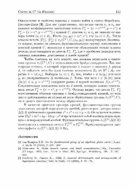
Curves in C2 (in Russian) 111

Îïðåäåëåíèå è ñâîéñòâà ïîðÿäêà ν ìîæíî íàéòè â ñòàòüå Ôîðñáåðãà-Ïàññàðå-Öèõà [3]. Äëÿ íàñ ñóùåñòâåííî, ÷òî öåëûå ÷èñëà νx è νy âû-ðàæàþò êîýôôèöèåíòû çàöåïëåíèÿ ïåòåëü Γνx = x = eu+it, y = ev èΓνy = x = eu, y = ev+it ñ êðèâîé C, ïðè÷åì νx è νy íå çàâèñÿò îò âû-áîðà òî÷êè (u, v) ∈ Eν . Ïóñòü (x0, y0) = (eu, ev), ãäå (u, v) ∈ Eν . Òîãäàêëàññû ïåòåëü [Γνx], [Γνy ] ∈ π1(C2 \ C, (x0, y0)) êîììóòèðóþò. Âîçíèêà-åò âîïðîñ, ìîæíî ëè îïèñàòü ôóíäàìåíòàëüíóþ ãðóïïó äîïîëíåíèÿ êïëîñêîé êðèâîé C, èñïîëüçóÿ â êà÷åñòâå îáðàçóþùèõ òîëüêî êëàññûïåòåëü, ïîëó÷àþùèõñÿ èç ïåòåëü Γνx, Γνy , ãäå ν ïðîáåãàåò ïîðÿäêè âñåõñâÿçíûõ êîìïîíåíò äîïîëíåíèÿ ê àìåáå êðèâîé?

×òîáû îòâåòèòü íà ýòîò âîïðîñ, ìû äîëæíû âåðíóòüñÿ ê îïèñà-íèþ ãðóïïû π1(C2 \ C) ñ èñïîëüçîâàíèåì áðýéä-ìîíîäðîìèè. Òàê êàêñòàðøàÿ ñòåïåíü, ñ êîòîðîé ïåðåìåííàÿ x âõîäèò â ïîëèíîì f , ðàâíàd, òî íàéäåòñÿ õîòÿ áû îäíà ñâÿçíàÿ êîìïîíåíòà Eeν èç R2 \ AC ïî-ðÿäêà ν = (d, νy). Âûáåðåì (u, v) ∈ Eeν òàê, ÷òîáû v 6= ln |yi| äëÿ âñåõyi èç äèñêðèìèíàíòà ∆ ïîëèíîìà f . Òîãäà äëÿ âñåõ t ∈ [0, 2π] äèñêln |x| 6 u, y = ev+it ñîäåðæèò ðîâíî d êîðíåé ïîëèíîìà f(x, ev+it).Ñëåäîâàòåëüíî îïðåäåëåíà êîñà èç d íèòåé, êîòîðóþ ìîæíî ñîïîñòà-âèòü ïåòëå Γeν

y = x = eu, y = ev+it. Îòñþäà âèäíî, ÷òî ïåòëè Γνx, Γνyåñòåñòâåííûì îáðàçîì ñâÿçàíû ñ áðýéä-ìîíîäðîìèåé êðèâîé, òî åñòüìîãóò ïðåòåíäîâàòü íå òîëüêî íà ðîëü îáðàçóþùèõ ãðóïïû π1(C2 \C),íî è äàâàòü ñîîòíîøåíèÿ ìåæäó îáðàçóþùèìè.

Â êà÷åñòâå ïðîñòîãî ïðèìåðà êðèâîé, ôóíäàìåíòàëüíàÿ ãðóïïàäîïîëíåíèÿ êîòîðîé îïðåäåëÿåòñÿ àìåáîé, ðàññìîòðèì äèñêðèìèíàíò∆[2, 3] êóáè÷åñêîãî óðàâíåíèÿ z3 +z2 +xz+y = 0. Îí çàäàåòñÿ ïîëèíî-ìîì 27y2+4x3+4y−18xy−x2 è ïðåäñòàâëÿåò ñîáîé êàñïèäàëüíóþ êðè-âóþ ñ íåâûðîæäåííîé àìåáîé. Ôóíäàìåíòàëüíàÿ ãðóïïà π1(C2\∆[2, 3])îïèñûâàåòñÿ ñ ïîìîùüþ ïåòåëü Γ(3,0)

x è Γ(0,2)y . Áðýéä-ìîíîäðîìèÿ äàåò

èçîìîðôèçì π1(C2 \∆[2, 3]) ∼= Br3.


[1] van Kampen E.R. On the fundamental group of an algebraic plane curve//Amer.J. Math. 55 (1933), P. 255 - 260.

[2] Moishezon B. Stable branch curves and braid monodromies//Alg. Geometry(Chicago, 1980), Lect. Notes in Math. 862, Springer, Heidelberg, 1981, P. 107 -192.

[3] Forsberg M., Passare M., Tsikh A. Laurent determinants and arrangements of

hyperplane amoebas//Adv. in Math. 151 (2000), P. 45 - 70.

LIST OF PARTICIPANTS AND AUTHORS

AKIAN Marianne,

INRIA, Domaine de Voluceau, B.P. 105, 78153 Le Chesnay Cedex, [email protected]

BAKLOUTI Ali,

Department of Mathematics, Faculty of Sciences at Sfax, Route de Soukra, 3038,Sfax, Tunisia. [email protected]

BELAVKIN Viacheslav P.,

School of Mathematical Sciences, Nottingham University, NG7 2RD, UnitedKingdom. [email protected]

BENIAMINOV Evgeny M. (Áåíèàìèíîâ Åâãåíèé Ìèõàéëîâè÷),Russian State University for the Humanities, Faculty of Mathematics,ul. Chayanova 15, Moscow, Russia. [email protected]

CHOURKIN Andrey V. (×óðêèí Àíäðåé Âàëåðüåâè÷),M.V. Lomonosov Moscow State University, Faculty of Physics, Chair of Quan-tum Statistics and Field Theory, 119992, Leninskie Gory, Moscow, [email protected]

DANILOV Vladimir I. (Äàíèëîâ Âëàäèìèð Èâàíîâè÷),CEMI RAS, Nahimovski prosp. 47, 117418, Moscow, [email protected]

FARHI Nadir,


FAYE Farba,

Department of Mathematics & Computer Science, UCAD, Dakar, [email protected]

FOCK Vladimir V. (Ôîê Âëàäèìèð Âëàäèìèðîâè÷),ITEP, B. Cheremushkinskaya 25, Moscow, Russia. [email protected]

GAUBERT Stephane,


GEL'FAND Alexander M. (Ãåëüôàíä Àëåêñàíäð Ìàðêîâè÷),Deln-Informatika Co., ul. Tkackaya 1, Moscow, [email protected]

GONCHAROV Alexander B.,

Brown University, Math. Department, 151 Thayer st., Providence, RI, [email protected]

GRBIC Tatjana (Ãðáè÷ Òàòjàíà),University of Novi Sad, Faculty of Technical Sciences,Trg Dositeja Obradovica 6, 21000 Novi Sad, Serbia. [email protected]

GULINSKY Oleg V. (Ãóëèíñêèé Îëåã Âèêòîðîâè÷),IPPI RAS, B. Karetny 1, Moscow, Russia. [email protected]

GUREVICH Dmitry,

LAMAV, Universite de Valenciennes,Le Mont Houy 59313 Valenciennes, France. [email protected]

GUTERMAN Alexander E. (Ãóòåðìàí Àëåêñàíäð Ýìèëüåâè÷),M.V. Lomonosov Moscow State University, Department of Mechanics and Math-ematics, Faculty of Higher Algebra, 119992 Leninskie Gory, Moscow, [email protected]

IGONIN Sergey,

Utrecht University, NL-3508 TA Utrecht,The Netherlands. [email protected]

ITENBERG Ilia,

IRMA, Universite Louis Pasteur, 7 rue Rene Descartes, 67084 Strasbourg Cedex,France. [email protected]

KARZANOV Alexander V. (Êàðçàíîâ Àëåêñàíäð Âèêòîðîâè÷),ISA RAS, prosp. 60-letiya Oktyabrya 6, 117312, Moscow, [email protected]

KHARLAMOV Vyacheslav,

IRMA, Universite Louis Pasteur, 7 rue Rene Descartes, 67084 Strasbourg Cedex,France. [email protected]

KIRSHTEYN Boris Kh. (Êèðøòåéí Áîðèñ Õàéìîâè÷),Deln-Informatika Co., ul. Tkackaya 1, Moscow, [email protected]

KOLOKOLTSOV Vassili N. (Êîëîêîëüöîâ Âàñèëèé Íèêèòè÷),Moscow Institute of Economics, Pecherskaya ul. 6/1, 129344, Moscow, and theUniversity of Warwick, Dept. of Statistics, Coventry CV4 7AL, Russia and

United Kingdom. [email protected]

KOSHEVOY Gleb A. (Êîøåâîé Ãëåá Àëåêñååâè÷),CEMI RAS, Nahimovski prosp. 47, 117418, Moscow, [email protected]

KOVAL Gennady V. (Êîâàëü Ãåííàäèé Âàñèëüåâè÷),M.V. Lomonosov Moscow State University, Faculty of Physics, Chair of Quan-tum Statistics and Field Theory, 119992, Leninskie Gory, Moscow, [email protected]

KUSHNER Alexey G. (Êóøíåð Àëåêñåé Ãóðüåâè÷),Astrakhan State University, ul. Tatischeva 20a, 414056, Astrakhan, [email protected]

KUTATELADZE Simon S. (Êóòàòåëàäçå Ñåìåí Ñàìñîíîâè÷),S.L. Sobolev Mathematical Institute, prosp. Koptyuga 4, 630090, Novosibirsk,Russia. [email protected]

LITVINOV Grigory L. (Ëèòâèíîâ Ãðèãîðèé Ëàçàðåâè÷),Independent University of Moscow, 119002, B. Vlasyevsky per. 11, Moscow,Russia. [email protected]

MASLOV Victor P. (Ìàñëîâ Âèêòîð Ïàâëîâè÷),M.V. Lomonosov Moscow State University, Faculty of Physics, Chair of Quan-tum Statistics and Field Theory, 119992, Leninskie Gory, Moscow, [email protected]

MCCAFFREY David,

7th oor, St. James building, 79 Oxford Street, Manchester M1 6SS, UnitedKingdom. [email protected]

MCENEANEY William M.,

Dept. of Mechanical and Aerospace Engineering, MC 0411, University ofCalifornia, San Diego 9500 Gilman Drive, La Jolla, CA 92093-0411, [email protected]

MIKHALKIN Evgeny N. (Ìèõàëêèí Åâãåíèé Íèêîëàåâè÷),Krasnoyarsk State Pedagogical University, 660049, ul. A. Lebedevoy 89,Krasnoyarsk, Russia. [email protected]

MOLCHANOV Vladimir F. (Ìîë÷àíîâ Âëàäèìèð Ôåäîðîâè÷),G.R. Derzhavin Tambov State University, 392000, ul. Internacionalnaya 33,Tambov, Russia. [email protected]

NITICA Viorel,

Institute of Mathematics of the Romanian Academy, P.O. Box 1-764,010702 Bucharest and Dept. of Mathematics, West Chester University, PA,Romania and USA. [email protected]

PAP Endre,

University of Novi Sad, Faculty of Sciences and Mathematics,Trg Dositeja Obradovica 4, 21000 Novi Sad, Serbia. [email protected]

PERSSON Ulf,

Chalmers University of Technology, 412 96 Goteborg, [email protected]

QUADRAT Jean-Pierre,


RASHKOVSKII Alexander Yu. (Ðàøêîâñêèé Àëåêñàíäð Þðüåâè÷),University of Stavanger, 4036 Stavanger, [email protected]

SERGEEV Serge N. (Ñåðãååâ Ñåðãåé Íèêîëàåâè÷),M.V. Lomonosov Moscow State University, Faculty of Physics, Chair of Quan-tum Statistics and Field Theory, 119992, Leninskie Gory, Moscow, [email protected]

SHPIZ Grigory B. (Øïèç Ãðèãîðèé Áîðèñîâè÷),Independent University of Moscow, 119002, B. Vlasyevsky per. 11, Moscow,Russia. [email protected]

SHUSTIN Eugenii,

School of Mathematical Sciences, Tel Aviv University, Ramat Aviv, Tel Aviv,69978, Israel. [email protected]

SHVEDOV Oleg Yu. (Øâåäîâ Îëåã Þðüåâè÷),M.V. Lomonosov Moscow State University, Faculty of Physics, Chair of Quan-tum Statistics and Field Theory, 119992, Leninskie Gory, Moscow, [email protected]

SINGER Ivan,

Institute of Mathematics of the Romanian Academy, P.O. Box 1-764,010702 Bucharest, Romania. [email protected]

SOBOLEVSKII Andre (Ñîáîëåâñêèé Àíäðåé Íèêîëàåâè÷),M.V. Lomonosov Moscow State University, Faculty of Physics, Chair of Quan-tum Statistics and Field Theory, 119992, Leninskie Gory, Moscow, [email protected]

STOYANOVSKY Alexander V. (Ñòîÿíîâñêèé Àëåêñàíäð Âàñèëüåâè÷),Independent University of Moscow, 119002, B. Vlasyevsky per. 11, Moscow,Russia. [email protected]

STRBOJA Mirjana (Øòðáîjà Ìèðjàíà),University of Novi Sad, Faculty of Sciences and Mathematics,Trg Dositeja Obradovica 4, 21000 Novi Sad, Serbia. [email protected]

THIAM Mamadou,

Department of Mathematics & Computer Science, UCAD, Dakar, [email protected]

TRUFFET Laurent,

Institut de Recherche en Communications et Cybernetique de Nantes, IRCCyNUMR-CNRS 6597, 1, rue de la Noe BP 92101 44321 Nantes Cedex, [email protected]

TSYKINA Svetlana V. (Öûêèíà Ñâåòëàíà Âèêòîðîâíà),G.R. Derzhavin Tambov State University, 392000, ul. Internacionalnaya 33,Tambov, Russia. [email protected]

ULVERT Roman V. (Óëüâåðò Ðîìàí Âèêòîðîâè÷),Siberian Federal University, Department of Mathematics and Informatics,660041, pr. Svobodnyi 79, Krasnoyarsk, Russia. [email protected]

WAGNEUR Edouard,Ecole Polytechnique de Montreal, C.P. 6079 Succ. Centre-ville, Montreal QuebecH3C 3A7, and GERAD, Montreal, Canada. [email protected]

WALSH Cormac,


ZNAMENSKAYA Oksana V. (Çíàìåíñêàÿ Îêñàíà Âèòàëüåâíà),Siberian Federal University, Department of Mathematics and Informatics,660041, pr. Svobodnyi 79, Krasnoyarsk, Russia. [email protected]

Documents

International Workshop - arxiv.org · 6 Victor P. Maslov It was was impossible at the time to implement this e ect in practice, which would have allowed to obtain a unimode laser,