Embed Size (px)
Citation preview

International Vehicle Emissions Modeling
Design And Measurements

IVE Modeling Goals
• Define low-cost, easy to use methodologies for developing key motor vehicle related data.
• Provide a sophisticated model that is:– Flexible and easy to use.– Adaptable to multiple international locations.– Useful for analyzing policy decisions and vehicle
growth impacts.– Provides a broad range of criteria, toxic, and global
warming pollutant data.

Results• Have developed data collection methodologies to
supplement local data that can be completed in 2-3 weeks using about 12-15 participants.
• Have completed development of a computer based emissions model that allows consideration of local geographic information, fleet technologies, and driving patterns.
• Criteria pollutants, toxic pollutants, and global warming gases can be estimated.

0
5
10
15
20
25
0.7 0.9 1.1 1.3 1.5
Air/Fuel Ratio (Lambda)
Rel
ativ
e E
mis
sio
ns
CO
HC
NOx
Emissions Compared to Air/Fuel Ratio
Stochiometric
Most Torque
Better Fuel Economy
Source: Bosch Automotive Handbook

0
2
4
6
8
10
12
14
16
0.7 0.8 0.9 1 1.1 1.2 1.3 1.4 1.5
Air/Fuel Ratio (Lambda)
Rela
tive E
mis
sio
ns
20 deg
30 deg
40 deg
50 deg
NOx Emissions and Ignition Timing
Highest Torque
Best Fuel Economy
Source: Bosch Automotive Handbook

Catalyst Efficiency verses Catalyst Temperature and Time
0%
10%
20%
30%
40%
50%
60%
70%
80%
90%
100%
0 100 200 300 400 500 600 700 800
Catalyst Temperature (deg C)
Cat
alys
t E
ffic
ienc
y
0%
10%
20%
30%
40%
50%
60%
70%
80%
90%
100%
0 20 40 60 80 100 120 140 160 180 200
Time (se c)
Cat
aly
st E
ffic
ienc
y

Vehicle Emissions Are Dynamic
• Change second by second.
• Depend on– Vehicle technology.– Engine operating parameters.– Temperature, altitude, and humidity.– Fuel characteristics

Keys To Vehicle Emissions

Engine Technology• Ignition Type and Compression Ratios
– Spark ignition, compression ignition, high or low compression ratios.
• Air Fuel Control– Carburetor, Single-Point or Multi-Point Fuel
Injection.– Oxygen Sensor/Computer
• Ignition Control– Mechanical, Computer

Evaporative Control
• Positive Crankcase Ventilation– Vapors from engine oil system collected and
fed to combustion cylinders
• Fuel Tank Vapor Capture– Carbon Canisters that regenerate when
engine is operated– Sealed fuel tank
• Improved Engine Seals

Tailpipe Control• Air pump
– Adds combustion air to tailpipe.
• 2-Way Catalyst (CO/VOC Control)– Catalyst design and active metal content.
• 3-Way Catalyst (CO/VOC/NOx Control)– Catalyst design and active metal content.
• Location of Catalyst near engine– Heats catalyst faster to provide emissions control
sooner
• Pre-capture pollutants during first few minutes of vehicle operation– Captures pollutants until catalyst is hot
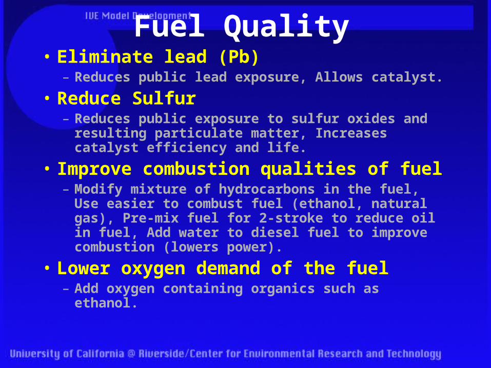
Fuel Quality• Eliminate lead (Pb)
– Reduces public lead exposure, Allows catalyst.
• Reduce Sulfur– Reduces public exposure to sulfur oxides and
resulting particulate matter, Increases catalyst efficiency and life.
• Improve combustion qualities of fuel– Modify mixture of hydrocarbons in the fuel, Use
easier to combust fuel (ethanol, natural gas), Pre-mix fuel for 2-stroke to reduce oil in fuel, Add water to diesel fuel to improve combustion (lowers power).
• Lower oxygen demand of the fuel– Add oxygen containing organics such as ethanol.

Local Geographic Parameters
• Temperature
• Altitude
• Humidity
• Road Grade

Emissions Broken Into Two Categories• Start-up emissions
– Excess emissions beyond normal hot-running emissions that occur while engine is warming up.
– Occur typically in the first 200 seconds of vehicle operation.
• Running emissions– Those emissions that occur during vehicle
operations including idle.– There are both running and start-up emissions
during the first 200 seconds of vehicle operation.

0
50000
100000
150000
200000
250000
300000
0 50 100 150 200 250 300 350
Time from Start (seconds)
CO
Em
iss
ion
s (
ug
/se
c)
Example of Start-Up Emissions
Carbon Monoxide
LEV Vehicle

0.00
2000.00
4000.00
6000.00
8000.00
10000.00
12000.00
0 50 100 150 200 250 300
Time from Start (seconds)
NO
(u
g/s
)Example of Start-Up Emissions (cont.)
Nitrogen Oxide
LEV Vehicle
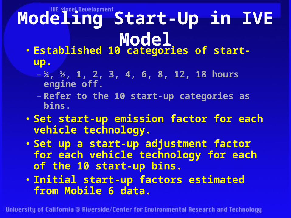
Modeling Start-Up in IVE Model• Established 10 categories of start-up.
– ¼, ½, 1, 2, 3, 4, 6, 8, 12, 18 hours engine off.– Refer to the 10 start-up categories as bins.
• Set start-up emission factor for each vehicle technology.
• Set up a start-up adjustment factor for each vehicle technology for each of the 10 start-up bins.
• Initial start-up factors estimated from Mobile 6 data.
Determination of Vehicle Start-Up Patterns

Measuring Start-Up Patterns
• Survey– Ask drivers to fill out forms about
daily driving habits.– Provide booklet to drivers to fill out
throughout the day.
• Instrumentation

Voltage Based Start-Up Monitor
Designed and built by Global Sustainable Systems Research
Voltage monitored in cigarette lighter.
VOCE Unit records second by second voltage that is used to determine driving times and start-up information.

US/ Chilean Start-Up Patterns
0%
5%
10%
15%
20%
25%
30%
35%
40%
Fra
ctio
n o
f Sta
rt-U
ps
0.06-0.5Hour
0.51-1.0Hour
1.1-2.0 Hour
2.1-3.0Hour
3.1-4.0Hour
4.1-5.0Hour
6.1-8.0Hour
8.1-12.0Hour
12.1-18.0Hour
>18.0Hour
Time Vehicle Shut-Off Before Start
Santiago Overall U.S. Comparison

Chilean Vehicle Starts by HourWeekday
Pre-Start Category Overall
6:00 to 10:00
10:00 to 14:00
14:00 to18:00
18:00 to 22:00
22:00 to 2:00
2:00 to 6:00
U.S. Comparison
0.25 Hour 38% 37% 47% 43% 34% 36% 60% 19%0.5 Hour 10% 5% 18% 13% 9% 5% 0% 17%1 Hour 12% 3% 9% 10% 19% 23% 0% 11%2 Hour 5% 0% 12% 5% 4% 9% 0% 11%3 Hour 7% 2% 2% 15% 4% 14% 0% 6%4 Hour 6% 3% 7% 3% 10% 9% 40% 10%6 Hour 4% 5% 0% 3% 5% 5% 0% 4%8 Hour 11% 29% 2% 8% 11% 0% 0% 4%12 Hour 5% 15% 2% 0% 2% 0% 0% 6%18 Hour 1% 2% 2% 3% 1% 0% 0% 12%Starts 6.3 23.8% 20.6% 14.3% 31.8% 7.9% 1.6% 7.0
WeekendPre-Start Category Overall
6:00 to 10:00
10:00 to 14:00
14:00 to18:00
18:00 to 22:00
22:00 to 2:00
2:00 to 6:00
U.S. Comparison
0.25 Hour 35% 33% 36% 45% 32% 34% 31% 19%0.5 Hour 14% 5% 20% 14% 11% 20% 0% 17%1 Hour 17% 7% 13% 16% 22% 20% 23% 11%2 Hour 4% 0% 3% 4% 5% 6% 8% 11%3 Hour 6% 0% 7% 6% 5% 6% 23% 6%4 Hour 5% 2% 1% 6% 9% 4% 15% 10%6 Hour 3% 7% 1% 0% 4% 4% 0% 4%8 Hour 8% 28% 5% 1% 7% 2% 0% 4%12 Hour 6% 12% 13% 4% 1% 4% 0% 6%18 Hour 3% 7% 1% 3% 3% 0% 0% 12%Starts 6.0 11.7% 25.0% 18.3% 28.4% 13.3% 3.3% 7.0

Distribution of Daily Passenger Vehicle Driving
0.0%
5.0%
10.0%
15.0%
20.0%
25.0%
30.0%
35.0%
40.0%
Fra
ctio
n o
f D
rivi
ng
06:00-10:00 10:00-14:00 14:00-18:00 18:00-22:00 22:00-02:00 02:00-06:00
Time Range
Weekday Weekend

Sample Running Emissions
0
20
40
60
80
100
120
1000 1050 1100 1150 1200 1250 1300
Time from Start (seconds)
CO
Em
issio
ns (
ug
/s)
0
5
10
15
20
25
30
35
40
45
50
CO Vehicle Speed

Sample Running Emissions (cont.)
0
20
40
60
80
100
120
140
160
180
200
1000 1050 1100 1150 1200 1250 1300
Time from Start (seconds)
NO
Em
iss
ion
s (
ug
/s)
0
5
10
15
20
25
30
35
40
45
50
NO Vehicle Speed

Development of Driving Factors
• Second by second emissions and associated driving data were reviewed to determine best driving factors to estimate emissions.
• Statistical analysis indicates that vehicle power requirement is the best overall predictor of emissions.

Vehicle Power DemandVSP (kW/ton) can be calculated for each second of data using
the following equation [Jimenez-Palacios, 1999]:
VSP = v[1.1a + 9.81 (atan(sin(grade)))+0.132] + 0.000302v3
grade = (ht=0 – ht=-1)/ v (t=-1to0) v = velocity (m/s) a = acceleration (m/s2) h = Altitude (m)
Engine Stress (unitless) = RPMIndex + (0.08 ton/kW)*PreaveragePower
PreaveragePower = Average(VSPt=-5sec to –25 sec) (kW/ton) RPMIndex = Velocityt=0/SpeedDivider (unitless) Minimum RPMIndex = 0.9
Engine stress is related to vehicle power load requirements over the past 20 seconds of operation and engine RPM:

Vehicle Emissions & Power DemandCO2 Emissions Increase Power Curves
0
1
2
3
4
5
6
7
8
0 5 10 15 20
Low Stress
Med Stress
High Stress
CO Emissions Increase Power Curves
0
50
100
150
200
250
0 5 10 15 20
Low Stress
Med Stress
High Stress
VOC Emissions Increase Power Curves
0
5
10
15
20
25
30
35
40
0 5 10 15 20
Low Stress
Med Stress
High Stress
NOx Emissions Increase Power Curves
0
2
4
6
8
10
12
14
16
18
0 5 10 15 20
Low Stress
Med Stress
High Stress

Estimates for the IVE Model• Divided driving patterns into 20 power bins.
– 15 power bins may be sufficient to represent power data.
• Established parameter called vehicle stress.– Weights Implied RPM and Pre-Power and
sums them to produce an index.– Weighting established by statistical analysis
to give the best emission results.– Pre-Power is least important and may
deserve to be dropped.– Three Stress bins were established.

Power Bins for IVE Model
• 60 total bins used for model.
• 3 stress bins and 20 power bins set up to estimate driving impacts on emissions.
• 60 bin process allows alternative binning modifications in future model improvements.

Advantage of Power Binning
• Power statistics easily drawn from measured vehicle speed patterns.
• Road grade and air conditioning loads can easily be included in the binning process.

IVE Model Uses 3 Key Input Files• Location file describes applicable
– Altitude, road grade(optional), temperature, humidity
– Diesel and gasoline fuel quality
– Driving and start patterns and amounts
• Fleet file describes applicable– Distribution of vehicle technologies (2 X 1243)
– Allows Normal Use and Multi-stop vehicles
• Country adjustment file describes applicable– Adjustments to base emission factors

Model Calculation Process

Model Calculation Process Allows
• Single or Multiple times of day
• Single or Multiple locations or links in an urban area
• Use of local emission factors
• Setup of independent adjustment calculations for each technology and pollutant

Location Page• Specifies data pertaining to the
immediate location including– General Information such as average
altitude, type of I/M program if any, fraction of persons using a/c at 80 deg F, fossil fuel characteristics.
– Hourly (or daily) data including driving patterns, average speeds, travel distance or time, temperature, humidity, start patterns, number of starts

Fleet Technologies• The IVE model allows selection of up to 1243
technologies categorized by vehicle type, size, fuel type, age and emissions control technology
• Several Default files are created for the IVE models from the MOBILE6 data
• Data has been collected for Santiago, Chile and Nairobi, Kenya
• Plans are underway to collect data in Kazakhstan, India, and Guatemala
• Data needs to be collected in China, Thailand, Philippines, Indonesia, and Malaysia

Vehicle Technology Classifications
Carburetor NonePre-Chamber
Inject.None
Carburetor / Mixer
None Carburetor NonePre-Chamber
Inject.None Carburetor None 2-Cycle, FI None
Carburetor 2-WayPre-Chamber
Inject.Improved
Carburetor / Mixer
2-Way Carburetor 2-Way Direct Injection Improved Carburetor2-Way /
EGR4-Cycle, Carb None
Carburetor2-Way /
EGRDirect Injection EGR+
Carburetor / Mixer
2-Way / EGR
Carburetor2-Way /
EGRDirect Injection EGR+ Carburetor
3-Way / EGR
4-Cycle, Carb Catalyst
Carburetor 3-Way FI PM Carburetor /
Mixer3-Way Carburetor 3-Way FI PM FI
3-Way / EGR
4-Cycle, FI None
Carburetor3-Way /
EGRFI PM/NOx
Carburetor / Mixer
3-Way / EGR
Carburetor3-Way /
EGRFI PM/NOx 4-Cycle, FI Catalyst
Single-Pt FI none FI EuroI Single-Pt FI 2-Way FI none FI EuroI
Single-Pt FInone / EGR
FI EuroII Single-Pt FI2-Way /
EGRFI 2-Way FI EuroII
Single-Pt FI 2-Way FI EuroIII Single-Pt FI 3-Way FI2-Way /
EGRFI EuroIII
Single-Pt FI2-Way /
EGRFI EuroIV Single-Pt FI
3-Way / EGR
FI 3-Way FI EuroIV
Single-Pt FI 3-Way FI Hybrid Multi-Pt FI 3-Way FI3-Way /
EGRFI EuroV
Single-Pt FI3-Way /
EGRMulti-Pt FI
3-Way / EGR
FI EuroI FI Hybrid
Multi-Pt FI none Multi-Pt FI3-Way /
EGRFI EuroII
Multi-Pt FInone / EGR
ZEV FI EuroIII
Multi-Pt FI 3-Way FI EuroIV
Multi-Pt FI3-Way /
EGRFI EuroV
Multi-Pt FI3-Way /
EGRMulti-Pt FI LEV
Multi-Pt FI ULEV
Multi-Pt FI SULEV
Multi-Pt FI EuroI
Multi-Pt FI EuroII
Multi-Pt FI EuroIII
Multi-Pt FI EuroIV
Multi-Pt FI Hybrid
Gasoline and Ethanol Motorcycles
Heavy Duty Gasoline Vehicles
Light Duty Gasoline Vehicles
Heavy Duty Diesel VehiclesHeavy Duty Vehicles
(Ethanol, Natural Gas, Propane, etc)
Light Duty Diesel VehiclesLight Duty Vehicles
(Ethanol, Natural Gas, Propane, retrofits, etc)

Each Technology Classification
• Has three size groups associated with it.• Has three use groups associated with it.• Thus, there are 9 sub-groups for each
technology classification.• There are also 45 user defined technologies.• Two technology groups are used. One is for
normal vehicles and the second is for multi-stop vehicles.

Load Effects (Road Grade and A/C)
•Road Grade can either be modeled Directly through the use of the driving patterns or a constant road grade for the entire link may be applied in the Location File. Valid grade inputs range from –14 to +14%•The change in Vehicle Specific Power associated with Road Grade and A/C use is applied to the driving corrections. •The fraction of travel in each VSP bin is prorated for each bin.Example: user inputs road grade of 2% and average velocity of 15m/s => +2.9kW/ton VSP increase. Since each VSP bin range is 4.1kW/tons, the
model would move 72% of the fleet up a bin.

Adjustments to Emission Factors
• Local emission measurements can be used to improve calculations.
• Adjustment page provided in model to correct base emission factors.
• 45 undefined technologies provided in model.

Determining Vehicle Fleet Technology Distributions

Registration Data
• California: vehicles registered each year.– California registration database divided by
ZIP code location for fleet by location.
• Problems with approach– ZIP code of registration address may not
represent actual location of vehicle operation.
– No time of day or day of week operations available.
– Often does not indicate vehicle use by age.

On-Road Evaluations
• Observers used to manually record road traffic– Vehicles missed with large number of vehicles.
– Only simple technology evaluations possible.
• Video tape option– Allows freeze-frame to make more accurate count.
– Second zoomed in camera allows improved technology identification.
• Applied to Los Angeles, Santiago, Nairobi

Video Taping of Traffic

Parking Lot Surveys
• Allow improved collection of vehicle parameters.
• Los Angeles studies show good agreement with on-road data.

Parking Lot Survey in Nairobi

Los Angeles Registration, Videotape, Parking Lot
Los Angeles County
0
20
40
60
80
100
Model Year
Perc
ent
DMV
SELEV
Unreg

Model Year Distributions
0.00%
2.00%
4.00%
6.00%
8.00%
10.00%
12.00%
14.00%
Fra
ctio
n/Y
ear
Pre 1980 1980-1989 1990-1992 1993-1995 1996-1998 1999-2001
Model Year Group
Nairobi Santiago US
Santiago Average = 6 yrs
US Average = 10 yrs
Nairobi Average = 12 yrs

General On-Road TechnologiesPassenger Veh. Trucks Buses Motorcycles
Buruburu (Kenya) 86.85% 9.77% 1.83% 1.55%Maipu (Chile) 90.71% 5.40% 3.30% 0.59%
Puente Hills (U.S.) 92.95% 6.02% 0.90% 0.12%
Central Nairobi (Kenya) 90.74% 3.06% 4.46% 1.75%Santiago (Chile) 83.36% 6.76% 8.14% 1.73%Riverside (U.S.) 96.41% 3.00% 0.45% 0.14%
Mathaiga (Kenya) 90.53% 5.28% 3.10% 1.09%Vitacura (Chile) 91.57% 1.91% 4.79% 1.74%
Yorba Linda (U.S.) 96.76% 2.68% 0.40% 0.16%
Overall Los Angeles 95.37% 3.90% 0.59% 0.14%
Overall Nairobi 89.37% 6.03% 3.13% 1.46%Overall Santiago 88.55% 4.69% 5.41% 1.35%

Passenger Vehicle Size Distribution
Location Small Medium LargeBuruburu 57.0% 39.0% 4.0%
Maipu 45.2% 50.3% 4.5%Central Nairobi 68.4% 27.3% 4.3%
Central Santiago 33.8% 59.8% 6.4%Mathaiga 40.4% 40.0% 19.6%Vitacura 23.7% 62.5% 13.8%Overall 44.8% 46.5% 8.8%

Vehicle Use in Santiago
y = -297.95x2 + 16734x
R2 = 0.9746
0
50000
100000
150000
200000
250000
0 5 10 15 20 25 30
Age of Vehicle (years)
Ac
cu
mu
late
d U
se
(K
m)

Vehicle Use in Nairobiy = -531.49x2 + 20494x
R2 = 0.8294
0
50,000
100,000
150,000
200,000
250,000
300,000
0 2 4 6 8 10 12 14 16 18 20
Age of Vehicles (years)
Od
om
eter
(K
ms)

Comparison of Vehicle Use
0
50,000
100,000
150,000
200,000
250,000
300,000
350,000
400,000
0 5 10 15 20 25 30
Santiago Nairobi LA
Acc
um
ula
ted
Dri
vin
g (k
m)
US=24,000 km/yr
Santiago=16,000 km/yr
Nairobi=17,000 km/yr
Determining Vehicle Driving Patterns

Objectives
• Develop a methodology for determining power demand on vehicle.– Must know vehicle speed and
acceleration second by second.
– Need to know road grade.
– Need to know air conditioning use.
Global Positioning Satellite Units• Easy to Use• Provide second by second speed, location, and
altitude.• Units combined with microprocessor and flash
memory to store up to one-week of driving data at a time.
• Problems– Loose satellites around tall buildings
– First 3 seconds of acceleration underestimated but then corrects.

Driving Data Collection

Driving Patterns in LA, Nairobi, and Santiago and
Associated Emissions

Driving Data Collection
• In three parts of urban area– Lower income, higher income, commercial
• On three road types– Major highway (freeway), major connecting
roads (arterial), residential streets.
• Each hour from 6am to 9pm
• Using three vehicles and drivers

Results: Velocity Trace for Santiago, Chile
0
20
40
60
80
100
120
0 100 200 300 400 500 600
Time (seconds)
Spe
ed (k
ph)
Freeway
Arterial
Residential

Results: Velocity Trace for Los Angeles, California
0
20
40
60
80
100
120
0 100 200 300 400 500 600
Time (seconds)
Spe
ed (k
ph)
Freeway
Arterial
Residential

Typical Bus Data (Santiago)
0
10
20
30
40
50
60
70
80
90
0 100 200 300 400 500 600
Time (sec)
Sp
eed
(k
ph
)

Comparison of Freeway Driving
0%
10%
20%
30%
40%
50%
60%
70%
Idle Fast Accel Mod Accel Slow Accel Fast Deccel Mod Deccel SlowDeccel
High Cruise Mod Cruise Slow Cruise
Trav
el F
requ
ency
(% T
ime)
Los Angeles, CA
Santiago, Chile
Nairobi, Kenya

Comparison of Arterial Driving
0%
10%
20%
30%
40%
50%
60%
Idle Fast Accel Mod Accel Slow Accel Fast Deccel Mod Deccel Slow Deccel High Cruise Mod Cruise Slow Cruise
Tra
vel F
req
ue
ncy
(%
Tim
e)
Los Angeles, CA
Santiago, Chile
Nairobi, Kenya

Results: Effect of Congestion on FreewaysS
anti
ago
Nai
robi
Los
Ang
eles
0%
5%
10%
15%
20%
25%
30%
35%
40%
45%
50%
Power Bin (kW/ton)
Fra
ctio
n o
f D
riv
ing
Freeflow
Moderate Congestion
Heavy Congestion
Low StressModerate Stress
High Stress
0%
5%
10%
15%
20%
25%
30%
35%
40%
45%
50%
Power Bin (kW/ton)
Fra
ctio
n o
f D
riv
ing
Freeflow
Moderate Congestion
Heavy Congestion
Low Stress Moderate Stress High Stress
0%
5%
10%
15%
20%
25%
30%
35%
40%
45%
50%
Power Bin (kW/ton)
Fra
ctio
n o
f D
riv
ing Freeflow
Moderate Congestion
Heavy Congestion
Low Stress Moderate Stress High Stress

CO Emissions Estimate for LEV
0
1
2
3
4
5
6
7
Freeflow Freeflow Moderate Heavy Freeflow Moderate Heavy
Residential Arterial Freeway
No
rma
lize
d E
mis
sio
ns
Nairobi
Santiago
Los Angeles
Emissions from LA4
cycle

HC Emissions Estimate for LEV
0.0
0.2
0.4
0.6
0.8
1.0
1.2
1.4
1.6
1.8
Freeflow Freeflow Moderate Heavy Freeflow Moderate Heavy
Residential Arterial Freeway
No
rma
lize
d E
mis
sio
ns
Nairobi
Santiago
Los Angeles
Emissions from LA4
cycle

NOx Emissions Estimate for LEV
0.0
0.5
1.0
1.5
2.0
2.5
Freeflow Freeflow Moderate Heavy Freeflow Moderate Heavy
Residential Arterial Freeway
No
rma
lize
d E
mis
sio
ns
Nairobi
Santiago
Los Angeles
Emissions from LA4
cycle

Demonstration of IVE Model

IVE Estimates for SantiagoCarbon Monoxide
0
10
20
30
40
50
60
70
0 2 4 6 8 10 12 14 16 18 20 22
Hour of Day
On
-Ro
ad E
mis
sio
ns
(to
ns/
ho
ur)
Weekday Weekend
Nitrogen Oxides
0
2
4
6
8
10
12
14
0 2 4 6 8 10 12 14 16 18 20 22
Hour of Day
On
-Ro
ad E
mis
sio
ns
(to
ns/
ho
ur)
Weekday Weekend