International Journal of Geographical ... - people.duke.edu

PLEASE SCROLL DOWN FOR ARTICLE

This article was downloaded by: [Duke University]On: 8 February 2011Access details: Access Details: [subscription number 930879418]Publisher Taylor & FrancisInforma Ltd Registered in England and Wales Registered Number: 1072954 Registered office: Mortimer House, 37-41 Mortimer Street, London W1T 3JH, UK

International Journal of Geographical Information SciencePublication details, including instructions for authors and subscription information:http://www.informaworld.com/smpp/title~content=t713599799

An object-oriented shared data model for GIS and distributed hydrologicmodelsMukesh Kumara; Gopal Bhatta; Christopher J. Duffya

a Department of Civil and Environmental Engineering 212 Sackett Bldg, Penn State University,University Park, PA, USA

Online publication date: 10 June 2010

To cite this Article Kumar, Mukesh , Bhatt, Gopal and Duffy, Christopher J.(2010) 'An object-oriented shared data modelfor GIS and distributed hydrologic models', International Journal of Geographical Information Science, 24: 7, 1061 — 1079To link to this Article: DOI: 10.1080/13658810903289460URL: http://dx.doi.org/10.1080/13658810903289460

Full terms and conditions of use: http://www.informaworld.com/terms-and-conditions-of-access.pdf

This article may be used for research, teaching and private study purposes. Any substantial orsystematic reproduction, re-distribution, re-selling, loan or sub-licensing, systematic supply ordistribution in any form to anyone is expressly forbidden.

The publisher does not give any warranty express or implied or make any representation that the contentswill be complete or accurate or up to date. The accuracy of any instructions, formulae and drug dosesshould be independently verified with primary sources. The publisher shall not be liable for any loss,actions, claims, proceedings, demand or costs or damages whatsoever or howsoever caused arising directlyor indirectly in connection with or arising out of the use of this material.

http://www.informaworld.com/smpp/title~content=t713599799

http://dx.doi.org/10.1080/13658810903289460

http://www.informaworld.com/terms-and-conditions-of-access.pdf

An object-oriented shared data model for GIS and distributedhydrologic models

Mukesh Kumar, Gopal Bhatt and Christopher J. Duffy*

Department of Civil and Environmental Engineering, 212 Sackett Bldg, Penn State University,University Park, PA 16802, USA

(Received 24 May 2008; final version received 26 August 2009)

Distributed physical models for the space–time distribution of water, energy, vegetation,and mass flow require new strategies for data representation, model domain decomposi-tion, a priori parameterization, and visualization. The geographic information system(GIS) has been traditionally used to accomplish these data management functionalities inhydrologic applications. However, the interaction between the data management toolsand the physical model are often loosely integrated and nondynamic. This is because (a)the data types, semantics, resolutions, and formats for the physical model system and thedistributed data or parameters may be different, with significant data preprocessingrequired before they can be shared; (b) the management tools may not be accessible orshared by the GIS and physical model; and (c) the individual systems may be operatingsystem dependent or are driven by proprietary data structures. The impediment toseamless data flow between the two software components has the effect of increasingthe model setup time and analysis time of model output results, and also makes itrestrictive to perform sophisticated numerical modeling procedures (real-time forecast-ing, sensitivity analysis, etc.) that utilize extensive GIS data. These limitations can beoffset to a large degree by developing an integrated software component that shares databetween the (hydrologic) model and the GIS modules. We contend that the prerequisitefor the development of such an integrated software component is a ‘shared data model’,which is designed using an object-oriented strategy. Here we present the design of such ashared data model taking into consideration the data type descriptions, identification ofdata classes, relationships, and constraints. The developed data model has been used as amethod base for developing a coupled GIS interface to Penn State Integrated HydrologicModel (PIHM), called PIHMgis.

Keywords: PIHM; PIHMgis; model GIS coupling; UML; hydrologic modeling

1. Introduction

Physics-based distributed hydrologic models (DHMs) simulate hydrologic state variables inspace and time while using information regarding heterogeneity in climate, land use,topography, and hydrogeology (Freeze and Harlan 1969, Kollet and Maxwell 2006).Because of the large number of physical parameters incorporated in such a model, intensivedata development and assignment are needed for accurate and efficient model simulations. Ageographic information system (GIS) has the ability to handle both spatial and nonspatialdata, and perform data management and analysis. However, it lacks sophisticated analytical

International Journal of Geographical Information ScienceVol. 24, No. 7, July 2010, 1061–1079

*Corresponding author. Email: [email protected]

ISSN 1365-8816 print/ISSN 1362-3087 online# 2010 Taylor & FrancisDOI: 10.1080/13658810903289460http://www.informaworld.com

Downloaded By: [Duke University] At: 16:57 8 February 2011

and modeling capabilities (Maidment 1993, Abel and Kilby 1994, Kopp 1996, Wilson et al.1996). On the other hand, the physical models generally lack the data organization anddevelopment functionalities. Moreover, the data structure they are based upon does notfacilitate close linkage to GIS and decision support system (DSS) (National ResearchCouncil 1999). This increases the model setup time, hinders the analysis of model outputresults, compounds data isolation, reduces data integrity, and limits concurrent access of databecause of broken data flow between the data, physical model, and DSSs. The problem isacute when dynamic interaction is required during the model simulation. A need to seamlesslylink individual GIS and physical modeling systems provides the motivation for this paper.

Important efforts in bridging the gap between a hydrologic model and a GIS include thedevelopment of Hydrologic Data Development System (HDDS; Smith andMaidment 1995)based on ARC/INFO, water and erosion prediction project (WEPP) interface on GRASS(Engel et al. 1993), an interface between ArcInfo and HECmodeling system (Hellweger andMaidment 1999), BASINS by EPA (Lahlou et al. 1998), SWAT by Di Luzio et al. (2002),inland waterway contaminant spills modeling interface (Martin 2002 and Martin et al.2004), and Watershed Modeling System (WMS; Nelson 1997). A detailed overview ofattempts to develop hydrologic models inside GIS is reviewed by Wilson (1999). We notethat all the above approaches were basically trying to ‘couple’ a GIS and a process-basedhydrologic model for efficient processing, storing, manipulating, and displaying of hydro-geological data. WMS was a major development and different from other attempts in that itwas a stand-alone GIS system totally dedicated to hydrologic application. The developmentof Arc Hydro (Maidment 2002) was another important step in defining an exhaustive datamodel for a hydrologic system and providing a framework for storing and preprocessing thegeospatial and temporal data in GIS. The developed data model provided rules for thestructure, relationships, and operations on data types often used in hydrologic modeling.McKinney and Cai (2002) went a step further in reducing the gap between GIS and modelsby outlining an object-oriented methodology to link GIS and water management models. Inthe process, they identified the methods and objects of the water management models thatcan be represented as the spatial and thematic characteristics in GIS. One criticism of objectorientation–based integration has been its susceptibility to produce monolithic systems thatneed recompilation and linking to create new versions, resulting in slowmodel development,evaluation, and testing by independent users (He et al. 2002). However, for cases where(high-frequency) dynamic interactions between data and the physical model are desired,such as in a fully coupled hydrologic model that uses temporally adaptive mesh refinement,alternative system integration implementations based on service orientation (Zhu 2009) andmodeling frameworks (Blind and Gregersen 2004) are slower. Object-oriented integrationbased on shared methods and data structure are relatively fast and robust (integrity preser-ving) in such situations.

In this paper we propose a robust integration methodology that facilitates seamless dataflow between the data and model functionalities, thus making interactions between themfluid and dynamic. The objective of this work is to lay the foundation for a fully integratedand extensible GIS–DHM system through a shared data model that can support both of them.The shared data model provides (a) flexibility of modification and customization, (b) ease ofaccess of GIS data structure by the hydrologic model, (c) richness for representing complexuser-defined spatial relations and data types, and (d) standardization easily applicable to newmodel settings and modeling goals. The data model has been developed using state-of-the-artcomputer programming concepts of object-oriented programming (OOP). We also discuss indetail the intermediate steps of designing the shared data model from a GIS data model. Theemphasis in this exercise is elucidating program design, not the coding details. The resulting

1062 M. Kumar et al.


data model supports an open-source coupled framework that serves as a GIS interface to PennState Integrated Hydrologic Model (PIHM) and is called PIHMgis (http://sourceforge.net/projects/pihmgis/). The strategy presented here shows that the concepts and capabilitiesunique to the coupling approach can easily be implemented in other GISs and DHMs.

2. Integration methodology

Efforts to couple GIS with hydrologic models generally follow either a loose, tight, orembedded coupling (Goodchild 1992, Nyerges 1993) strategy (see Table 1). Watkins et al.(1996) and Paniconi et al. (1999) have discussed in detail the relative advantages anddisadvantages of coupling in terms of watershed decomposition, sensitivity and uncertaintyanalysis, parameter estimation, and representation of the watershed. Loose coupling is proneto data inconsistency, information loss, and redundancy, leading to increased model setuptime. At the same time, loosely coupled approaches are much simpler to design and program.At the other extreme, embedded coupling can leave the code inertial to change because of itslarge and complex structure (Goodchild 1992, Fedra 1996). Nonetheless, embedded cou-pling provides the dynamic ability to visualize and suspend ongoing simulations, queryintermediate results, investigate key spatial/temporal relations, and even modify the under-lying hydrologic model parameters (Bennett 1997).

From our point of view both tight and embedded coupling strategies offer the necessarydegree of sharing between GIS and hydrologic model for efficient data query, storage,transfer, and retrieval. We also note (from Table 1) that both coupling strategies underscorethe existence of a shared data model in their implementation. Clearly, the integration of GIStools and simulation models should first address the conceptual need of a shared data modelthat is implemented on top of a common data and method base. In order to design such a

Table 1. Characteristics of different levels of integration between a GIS and a hydrologic model.

Coupling level

Characteristics Loose Tight integration Embedding

Shared user interface · p pShared data andmethod base

· p p

Intra-simulationmodelmodification

· · p

Intra-simulationquery and control

· · p

Above translates to!

l Distinct GIS andhydrologic modelingpackages withindividual interfaces

l Information sharingthrough file exchangewhich can be tediousand error prone

l Underlying advantageis: different packagesfacilitate independentdevelopment

l Data exchange isautomatic

l Merges different toolsin a single powerfulsystem

l Avoids inconsistencyand data lossoriginating fromredundancy andheterogeneity ofmethod base

l Steerable numericalsimulation in termspossibility of changesin parameter orprocesses whilerunning

l Significantly complexprogramming and datamanagement

l Changes to the code arenot easy because of itsmonolithic structure

International Journal of Geographical Information Science 1063


shared data model, we follow a four-step approach. First we carry out identification andclassification of the various data types that form the hydrologic system (Section 3). Then wedesign the object-oriented data model for the data types identified in the previous step(Section 4). In the third step, we study the hydrologic model structure in terms of its dataneeds and adjacency relationships (Section 5). Finally, re-representation of the GIS datamodel classes to conform to the DHM data structure is carried out (Section 6). Next wediscuss in detail the design steps of the shared data model.

3. Conceptual classification of raw hydrologic data

A hydrologic model domain encompasses a wide range of hydraulic, hydrologic, climatic,and geologic data, including topography, rivers, soil, geology, vegetation, land use, weather,observation wells, and fractures. A conceptual classification of the raw hydrologic dataneeds to incorporate data of different origins, representation types, and scales.

Figure 1 illustrates a hierarchical categorization of real data typically required in hydrologicmodels. The design is intended to incorporate spatially heterogeneous thematic data typesalong with associated time series data, derived data, and attributes. The data types can bedefined as field based and object based (Couclelis 1992, Goodchild 1992). Field-based datadefine a spatial (or temporal) framework consisting of a set of locations related to each otherby (temporal) distance, direction, and contiguity (Galton 2001). Object-based data are collec-tion of individual entities that are characterized by geometry, topology, and nonspatial attributevalues (Heuvelink 1998). Spatial information to these entities is explicitly defined either asattributes or as a function of location that is inherent in a point, line, or polygon. We note thatthis kind of distinction in GIS features has been traditionally associated with raster and vectordata only. However, here we extend the concept of field data by considering it as a ‘continuousconcept’ whose unitary element exists either in space or time with respective entity informa-tion attached to it. For example, a unit element of any tessellation, like a grid or a TIN(triangular regular network), has an associated value that defines a property/characteristic

Figure 1. Conceptual classification of existing GIS data types relevant to hydrologic modeling.



magnitude/value anywhere within the field boundary. Similarly for a time series, there is avalue attached to any instant in the time series.

Figure 1 shows further subclassification of ‘field’ and ‘object’ data types that are relevantto hydrologic modeling. An object consists of points, line, and polygons. The fundamentalscope of the object subdata types has been extended in order to incorporate complex features(made up of multiple simple features) and the dynamic nature of observer and observables.We classify points as static and floating depending on their primary existence in space ortime. For example, a static point can be identified by a location at which time series data suchas wind speeds are being observed. On the other hand, an example of a floating point can be avolunteer in a soil moisture measurement field campaign who goes around the field takingsoil moisture samples at different locations. In the former case, the observer is fixed in spaceand is observing state in time while in the latter case a continuous time clock is fixed to theobserver while he/she moves around and takes sporadic samples at different locations. Staticpoints have been further subcategorized into isotropic and anisotropic points. Anisotropicpoints are locations whose entity attributes need information regarding direction and mag-nitude and possibly magnitude changing with direction (e.g., a second-rank tensor). Anexample of an anisotropic property representation at a point is hydraulic conductivity(Freeze and Cherry 1979). Line objects have been subcategorized into standard two-dimensional (2D) and 3D lines. The 3D polylines are made up of line segments that existin three dimensions, for example, an underground pipe network for drainage/wasteremovals, etc., which can change directions/planes in three dimensions at junctions.Polygon objects have been subcategorized into static and floating polygons. Floatingpolygons are bounded regions whose areas changes in time, such as a flooded region or alake. Field objects have been subclassified into tessellations (spatial) and time series(temporal) components. The unitary elements of tessellations define units of spaces withentity information attached to it.

The conceptual representation discussed above is generic and acts as a template that canbe populated by new data. Next we try to formally represent the data types in classes andidentify their attributes and their relationships with other classes.

4. Hydrologic data model design

A hydrologic data model is a formal representation of the real world that provides a standardstructure for storage, sharing, and exchange of data independent of the software environmentand programming languages. It provides a simplified abstraction of reality by (a) isolatingreal-world hydrologic objects into independent classes, (b) removing redundant classobjects, (c) defining relationships between independent classes, and (d) defining integrityconstraints on them.

The design of a hydrologic data model is performed keeping in mind the range ofrequired data types (see Figure 1) and their relationships among themselves (Wright et al.2007). Some data, such as elevation and soil properties, vary continuously in space whileothers like observed streamflow vary continuously in time. The representation of data alsochanges depending on the scale of interest. On a coarse scale the stream channel can berepresented as a 1D curvilinear object, while on a finer scale it can be considered as a 3Dtopographic section with width, depth, and length. For longer timescales such as climatechange or landscape evolution studies, the stream channel representation will also need atime identifier in addition to width, depth, and length attributes. These are necessary in orderto track the changes in shape over time due to erosion/deposition on the riverbed or banks.This means that the designed data model (a) must have the flexibility to incorporate different



representations of the same object at different scales, (b) should be extensiblewith a potentialto incrementally enrich it with new data types and construct complex objects, and (c) shouldbe robust and adaptable to changing hydrologic conditions by using different instances of asingle object (reusability). Maximum information, minimum data redundancy, reduction ofstorage capacity, and optimum retrievability of data for analysis are the desired objectives inthe design process. All these characteristics are sufficed by designing the data model usingobject-oriented concepts of inheritance, polymorphism, and encapsulation.

The object-oriented data modeling strategy provides a formal definition of objects, theirattributes and behaviors, and the operations that can be performed on them (Milne et al.1993, Alonso and El Abbadi 1994, Raper and Livingston 1995). Features sharing a set ofattributes and methods are clustered into a single class. Each instance of a class is called a datamodel object. An example of a class is a line feature and one of its instances is a river. Attributefields of the river line are an integer identifier, number of line segments, and start and end pointsof each segment. Methods are the functions that define the interaction of objects to the outsideworld. For example, calculation of total flowvolumebyusing the river dimension attributes is amethod associated with the river object. While every object in a class shares some of the sameset of attributes andmethods, theymay have additional properties attached to them. In additionto descriptions about objects, its attributes, and behaviors, the data model also explains therelationship between classes. For example, in order to account for flow and interactionsbetween each river segment and the watershed, and also to streamline query and storage, adefinition of (topological) relationships between classes is needed. Generalization, association,and aggregation are the three main relationships that have been implemented in the datamodel. The generalization relationship connects a child class to a base class using object-oriented ‘inheritance’ mechanism. The subclasses of a base class share many propertiesbetween themselves while separating from each other on the basis of new ‘identity’ proper-ties. Association shows the relationship between instances of classes that exist either in timeor in space. These linkages are either bidirectional, which means that both of the connectingclasses are aware of the relationship with each other, or unidirectional, where only one of theclasses knows about the relationship. This relationship markedly simplifies and clarifies thedata model, and minimizes redundancy in definitions, access, and storage. The developeddata model also uses another type of linkage, called reflexive association. This linkage relatesdifferent instances of the same class. Aggregation relationships have been implemented toexplain the interaction of individual parts/components (simple objects) to a complex object.

The formal static structural representation of data model classes and their attributes andrelationship is done using three-compartment Unified Modeling Language (UML) classdiagrams (shown in Figure 2a). UML class diagrams provide a programminglanguage–independent view of the static structure and behavior of classes. We note that

Figure 2. (a) Three-compartment structure of class icons. Options listed inside curly or large bracketsare optional. (b) Cardinality/multiplicity notation of relationships in a class diagram.



since the relationship between classes can be one-to-one or one-to-many, each relationshiprepresentation appropriately indicates the multiplicity of instances (examples shown inFigure 2b). In order to define the directionality in relationships between classes, UMLclass diagrams follow standardized notations. Generalization relationships are representedby line drawn from a child class to a base class with a white, solid arrow at the end.Unidirectional associations are represented by single-ended arrowheads where the classfrom which the arrow initiates is the class which has knowledge of the relationship. Theaggregation relationship is denoted by a white diamond (for the aggregate class) on one endof the link and arrow (for the ‘part’ class) on the other.

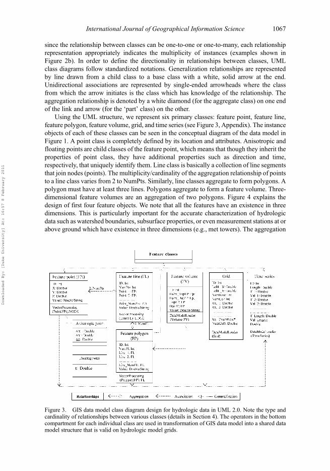
Using the UML structure, we represent six primary classes: feature point, feature line,feature polygon, feature volume, grid, and time series (see Figure 3, Appendix). The instanceobjects of each of these classes can be seen in the conceptual diagram of the data model inFigure 1. A point class is completely defined by its location and attributes. Anisotropic andfloating points are child classes of the feature point, which means that though they inherit theproperties of point class, they have additional properties such as direction and time,respectively, that uniquely identify them. Line class is basically a collection of line segmentsthat join nodes (points). The multiplicity/cardinality of the aggregation relationship of pointsto a line class varies from 2 to NumPts. Similarly, line classes aggregate to form polygons. Apolygon must have at least three lines. Polygons aggregate to form a feature volume. Three-dimensional feature volumes are an aggregation of two polygons. Figure 4 explains thedesign of first four feature objects. We note that all the features have an existence in threedimensions. This is particularly important for the accurate characterization of hydrologicdata such as watershed boundaries, subsurface properties, or evenmeasurement stations at orabove ground which have existence in three dimensions (e.g., met towers). The aggregation

Figure 3. GIS data model class diagram design for hydrologic data in UML 2.0. Note the type andcardinality of relationships between various classes (details in Section 4). The operators in the bottomcompartment for each individual class are used in transformation of GIS data model into a shared datamodel structure that is valid on hydrologic model grids.



relationships show how the traditional 2D simple objects like points and lines are used tomake a composite higher-dimension complex feature. One such example is the descriptionof an underground water pipe network, which is basically a collection of straight pipes thatzigzag through the subsurface in various planes. We note that the directionality (clockwise orcounterclockwise) of feature line sequence or of connections between polygons is inherentlydefined by the definition of a feature polygon or feature volume, respectively. Figure 3 alsoshows details of a time series data class, which is related to the feature objects throughunidirectional association.

The developed hydrologic data model acts as a transitional formal representation thatbridges the gap between the raw data types and their seamless assimilation in hydrologicapplications. Independently, the data model serves as a template to store and organize rawhydrologic data in GIS. For the data model to be used seamlessly in hydrologic modeling, thedata structure and relationships need to be modified such that they support representation ofdata and relationships on a hydrologic model grid. The eventual goal of course is to have ashared data model that can fully describe the hydrologic GIS data objects (shown inFigure 3) as well as their representational complement in the hydrologic model.

5. Hydrologic model structure: process representation and adjacency relationships

The conceptualization of process interactions and the shape and adjacency property of unitelements in the model grid control the design of the hydrologic model data structure. Herewe highlight the data and topological needs of the hydrologic model data structure vis-a-vis afinite volume–based PIHM (Kumar 2009, Qu and Duffy 2007). We reiterate that all the stepstaken are generic and can be used as a template in other GIS–hydrologic model coupling

Figure 4. Feature object designs for (a) point, (b) polyline, (c) polygon, and (d) volume. Note theimplicitness of the ‘sequence of constructs’ in feature polygon and feature volume design. Forexample, (c) shows that edge polylines of the polygon are always listed in clockwise direction.Similarly, definition of a 3D feature necessitates identification of a pivot point and boundary polygonsin a particular sequence. Note that the identification of one point from both top and bottom polygon indesign of feature volume is done in order to pivot the connection sequence of the nodes of the twopolygons which results in a 3D feature.



efforts that are based on different mesh decomposition strategies (e.g., structured meshes forfinite difference models). Next we highlight how the representation of physical processesand discretization of the model domain influences the hydrologic model data structure.

5.1. Physical process interaction

PIHM is a finite volume–based integrated hydrologic model. It simulates multiple physicalstates on discretized elements (also called model kernel) of a watershed domain by solvingsemi-discrete form of ordinary differential equations (ODEs) (Leveque 2002) given by

d�wdt¼X2

k¼1Qk �

X3

i¼1Qi (1)

where �w is interpreted as the volumetric storage (L3),Qi is the net volumetric flux through the(three) sides of the control volume, andQk is the net volumetric flux through upper and lowerboundaries. Details of the individual differential equations [of the form shown in Equation(1)] corresponding to each hydrologic processes, such as channel flow, overland flow,unsaturated zone storage, groundwater flow, interception storage, and snow melt, can bereferred to in Qu and Duffy (2007). The critical point to note here is that solutions of ODEs

Table 2. Data requirements for calculation of physical states on a model kernel at any simulation time.

Process Data support

Channel flow Head in adjacent triangular elements, head in river segment downstream andupstream, initial head value at the start of simulation, precipitation,evaporation, Manning’s coefficient, coefficient of discharge for weir flowacross river bank, elevation of end nodes of river segment, leakage coefficient,subsurface flow head in adjacent triangles, boundary conditions

Note: Head! overland fow (unless specified otherwise)Overland flow Head in neighboring elements, head in river segment (if river is neighbor to the

prismatic cell), initial head value, net precipitation, evapotraspiration, elevationof nodes of triangular element, boundary conditions

Note: Head! overland flowUnsaturated flow Capillary flow, initial head value, subsurface flow head, infiltration, hydraulic

conductivity, evapotranspiration, root uptake, soil porosity, van Genuchten soilparameters, boundary conditions

Note: Head! unsaturated flowGroundwater flow Head in adjacent triangles, initial head value, capillary flow, hydraulic

conductivity of the elements and its neighbors, bedrock depth, soil porosity,van Genuchten soil parameters, boundary conditions

Note: Head! groundwater flowInterception Interception storage capacity, precipitation, LAI, evapotranspiration, initial

interceptionSnow melt Initial snow depth, initial snow density, initial snow surface layer temperature,

initial average snow cover temperature, average snow liquid water content, netsolar radiation, incoming thermal radiation, air temperature, vapor pressure,wind speed, soil temperature, precipitation

Infiltration Overland flow head, unsaturated soil moisture, hydraulic conductivity, porosity,macropore, precipitation rate, maximum infiltration capacity

Evapotranspiration Wind speed, humidity, net radiation, soil heat flux, vapor pressure deficit, meanair density, interception storage capacity, LAI, soil saturation, atmosphericresistance, stomatal resistance, vegetation fraction, unsaturated zone saturation



for overland and groundwater flow depths depend on the head in adjacent kernels (Qu andDuffy 2007). Similarly, channel head is dependent on lateral fluxes from upstream anddownstream channel sections, and the watershed. This means that a design of the hydrologicmodel data structure must incorporate the topological relationship between neighboring unitelements. In addition to these relationships, Table 2 also lists the data requirements forcalculation of each physical state on every model kernel at any time. An inclusive hydrologicmodel data structure will account for the data requirements at all times.

The hydrologic model data structure is also influenced by the shape and adjacency ofunit elements, which are in turn defined by the choice of domain decomposition (structuredand unstructured) and numerical solution strategy (finite element, difference, or volume)employed in modeling.

5.2. Domain decomposition

PIHM uses unstructured meshes to decompose the domain. The individual unit controlvolume elements are either prismatic (for watershed elements) or trapezoidal/cuboidal (forriver elements). The flux exchange in prismatic elements takes place through five boundaryfaces (Kumar 2009). If a model uses structured grids to decompose the domain, then thenumber of faces across which flux exchange can potentially take place in three dimensionswill be equal to 6. So the shape of the unit element also determines how the relationshipsbetween neighboring elements need to be represented in a hydrologic model data structure.We note that the unstructured mesh decomposition poses additional challenges in the designof a hydrologic model data structure, particularly in terms of definition of topologicalrelationships, compared to structured grids, where the neighbors are implicitly characterizedby the decomposition itself.

With the object-oriented hydrologic data model in place (Section 4) and the spatialrelationships and parameter definitions for the hydrologic model identified (in this section),the last step in shared data model design is to represent the hydrologic GIS data types and thehydrologic model structure using the same feature classes, thus providing an automaticconnection between GIS and the hydrologic model. The next section discusses the design ofthis shared data model.

6. Shared data model design

The shared data model captures the spatial structure of hydrographic features and temporalobjects by identifying six classes: node, element, channel, soil, land cover, and time series(shown in Figure 5). These classes are representational complements of the six GIS datamodel classes (see Figure 3) and can be obtained by applying appropriate transformations orredefinitions. The relevant geometric, spatial, and topological transformations performed onGIS data types are shown in Figure 6. By generating mesh decomposition using points andlines as constraints (more details in Kumar et al. 2009), nodes of the triangles automaticallyact as feature points and edges of the triangles act as feature lines. Properties and attributes ofboundaries of the feature polygon are assigned to the element edges after converting thepolygons to polylines and then to lines. Attributes of the feature polygons and featurevolumes are geographically registered to the triangular elements. We note that all the re-representations of hydrologic GIS data types are ‘loss-less’ mappings, implying that they arereversible. By aggregating element edges, channels, or elements based on their attributeproperties, we can revert back from a shared data model class to the original GIS dataobjects. The operators used in re-representation of classes are shown over the lines



connecting the source and result classes in Figure 6. These operators are also listed as‘methods’ (in the bottom-most compartment) in the GIS data model class diagrams (seeFigure 3). The name of each of these operators is self-explanatory for their functions. Wenote that the dotted line in the transformation diagram indicates the intermediate results.

Figure 5 also shows the aggregation, unidirectional association, reflexive association,and generalization relationships supported in the shared data model. An element classrepresents a discretized triangular element in two dimensions and a prismatic element inthree dimensions, and is defined by six nodal locations listed in a clockwise direction at twolevels. The prismatic element has five neighbors – three on the sides and one each at the topand the bottom.We note that neighbors of an element also belong to an element class and thisrecursive relationship is captured by reflexive association. The cardinality of this relation-ship is 1 to 5, which means that there has to be at least 1 neighboring element to an elementobject. A maximum cardinality of 5 denotes that a 3D element can have a total of 3 lateral

Figure 5. Shared data model class diagram design for GIS–hydrologic model coupling in UML 2.0.Note the type and cardinality of relationships between various classes (details in Section 6).



and 2 vertical neighbors. A channel class is defined by the two end nodes and neighboringelements on the either side of channel. Each channel segment is also composed of anupstream and downstream channel segment, which is captured by a reflexive association.We note that the multiplicity of this relationship varies from 0 to any integer value. Thismeans that a channel segment can stand alone in the watershed with no upstream ordownstream channels. A channel is also bidirectionally associated with an element with amultiplicity of 1 to 2. This translates to existence of at least 1 neighboring triangular elementto a channel segment. Bidirectionality ensures that both element and channel are aware ofthis topological relationship. These relations are fundamentally important for spatial integ-rity of the hydrologic modeling framework. Each element class is also associated with soil,land cover, and time series class. This ensures clean and efficient assignment of properties toeach element. Similarly the channel is associated to bed property and shape classes. The soilclass contains several attribute fields such as hydraulic conductivities and van Genuchtenequation soil retention parameters (van Genuchten 1980). Attributes of the land cover classare root zone depth, albedo, and photosynthetically active radiation from each land covertype. We note that precipitation, temperature, humidity, incoming solar radiation, ground

GIS data model classes Shared data modelclasses

Feature point (FPt) Node

Element edge

Channel

Element

Time series

Feature polygon (FP)

Feature volume (FV)

Grid

Time series

Feature line (FL)

Vector processing: split line at nodes

Vector processing: polygon to line

Data model loader: topology definition

Vector processing: constraint assignment

Vector processing: constraint assignment

Data model loader: attributes assignment

Data model loader: forcings assignment

Figure 6. Class re-representation diagram showing the transformation of a GIS-based data modelclasses into classes identified in shared data model design. The arrows originate from each individualGIS data model class and end in the corresponding complement shared data model class. Operators/functions that perform this transformation are shown along the arrows. Dotted arrows representintermediate transformation operations.



heat flux, vapor pressure, leaf area index (LAI), vegetation fraction, wind velocity, time-dependent boundary conditions, and the observed and simulated state variables are allinstances or child objects to the time series class. Names of the operators shown inFigure 5 are self-explanatory regarding their functions. These operators are concernedwith derivation of geometric properties of triangular elements and channels or with thecalculation of rate of change of state variables with time. The definitions of various functionsare given in the Appendix.

The shared data model design is tested in the development of a coupled GIS–hydrologicmodeling system. The integrated software is an open-source, platform-independent, exten-sible, and ‘tightly coupled’ integrated GIS interface to PIHM and is referred to as PIHMgis.

7. PIHMgis

PIHMgis is an integrated and extensible GIS system with data management, analysis, datamodeling, unstructured mesh generation, visualization, and distributed PIHM modelingcapabilities. The underlying philosophy of this integrated system is a shared geodatamodel between GIS and PIHM, which was developed in the previous sections. The shareddata model makes it possible to handle the complexity of the representation structures, datatypes, model simulations, and analysis of results. The graphic interface component ofPIHMgis has been written in Qt and C++, which support object-oriented class structuresin programming. PIHMgis sits on an open-source Qgis engine (http://www.qgis.org) and hasbeen integrated as pluggable software. The interface and the source code can be downloadedfrom http://www.pihm.psu.edu/pihmgis_downloads.html.

The architectural framework of the interface is shown in Figure 7. The directionality ofthe arrows indicates the possible flow of output from one method to another. The flow ofactions between different class objects in PIHMgis can be shown using an object-orientedUML collaboration diagram (Figure 8). These diagrams represent both the static and the

Figure 7. Architectural framework of PIHMgis. Directionality of the arrows indicates the possibleflow of output from one module to another.



Figure8.

Collabo

ration

diagramshow

ingthedy

namicactivitysequ

ence

ofclassesinPIH

Mgis.The

rectangles

deno

tetheclassinstance,the

directionalityof

arrows

deno

testheflow

ofaction

,and

nested

numbering

keepstrackof

thesequ

ence

ofop

erations

inaglob

alfram

ework.Anexam

pleof

ahierarchicalnestingsequ

ence

is1!

1.1!

1.1.1.

Shadedbo

xesdeno

tetheindepend

entinitiation

(trigg

er)of

operations.



dynamic behavior of the system by representing collaboration (simple associations) betweenobjects and mapping the sequence of messages they share between them. The rectangles in thediagram enclose the class and its instance (separated by a colon), and the links betweenrectangles represent the collaborations (communications) between classes. The chronologicallabeling of the messages between class objects describes the sequence in which actions areexecuted. The first communication initiated by the integrated system is from the object fromwhere message 1.0 is released. In order to track the messages/actions that are hierarchicallyassociated with a parent object, a nested numbering of messages is performed. Figure 8 showsthat a full hydrologic modeling exercise can be carried out in PIHMgis by directly acting uponthe raw data types represented in the shared data model, merely by launching a sequence ofmessages (commands). Starting with digital elevation model raster data, which is an instanceof grid class, raster processing operations result in delineation of watersheds, definition ofstreams, and extraction of very important points (VIPs). Avector processing tool with polylinereconditioning algorithms simplifies and splits the watershed boundaries and channel seg-ments. Thereafter, vector merging of all the available feature layers is performed to create aspatial support for generating constrained domain decomposition. Details about the need ofvector processing steps and how they aid flexible domain decompositions are in Kumar et al.(2009). Once domain decomposition has been performed, topology definitions and fieldassignment of properties, and initialization of state variable on eachmodel kernel is performed.A numerical solver module formalizes all the ODEs in each model kernel in the form ofy0 ¼ f ðyÞ and then solves the system iteratively. Output results in the form of spatial and timeseries plots are displayed in the visualization toolkit integrated in PIHMgis. Details about allthe operator functions in the PIHMgis toolkits are discussed in Bhatt et al. (2008).

8. Advantages of shared data model for GIS–hydrologic model coupling

A shared database, and relationships and schemata betweenGIS and the hydrologic model reducethemodel setup time, enhance the data integrity, and streamline themodel simulations. As a result,the integrated system simulates the model states accurately and efficiently, steers simulations, andconveniently manages, analyzes, and displays data used and produced by the model. The uniqueadvantages of coupling based on a shared data model development are discussed next.

8.1. Enhanced accuracy and computational efficiency

As mentioned in Section 6, the hydrologic model grids supported by the shared data modelare generated by using GIS points, polylines, and polygons as constraints. The uniqueadvantage of using GIS objects as constraints for decomposition is that the resultingmodel grid can be designed to follow the edges of a single property type (such as soil,land cover, geology, and vegetation). This maintains the data integrity and limits theintroduction of additional data uncertainty arising from statistical averaging of multipleclass themes within a model grid (Kumar et al. 2009). Comparatively, structured griddecomposition will always have a large number of cells with mixed themes. For the sameorder of accuracy of representation of both raster and vector data, constrained decomposi-tions also use a smaller number of cells (or computational elements) relative to structuredmeshes (Kumar et al. 2009), thus resulting in computational efficiency. Similarly if observa-tion stations (point objects) are used as a constraint in decomposition, hydrologic states canbe predicted exactly at the observation stations. The georeferential integrity inherent in theshared data model minimizes any errors during comparison of observed and predicted states,which creep in due to interpolation of prediction variables to the observation locations.



8.2. Storage efficiency

In any watershed model, there are a limited number of parameters and forcing types(e.g., soil, land cover, and precipitation) that are needed to define each hydrologic propertyover the domain. This translates to storage efficiency at two levels in a shared data modelapproach. First, the efficiency is gained through storage of (soil or forcing) properties asrelational objects, which also ensures that these properties are accessible to both the GIS andthe hydrologic model. For example, instead of storing all the nine soil attribute parameters(floating type numbers) as separate grids, we are able to store them as a single layer of soiltypes (an integer attribute of element class) with associative relations defined for all the nineattributes of soil class. The compression is even more significant in storage of forcing timeseries, such as those of precipitation, Ppt, and temperature, T. Rather than storing the forcinggrid at numerous time steps (e.g., satellite images of time series variables such as tempera-ture), the precipitation-type attribute for each element class is associated with a precipitationmagnitude within a time series class. The associative relationships limit the data redundancyby avoiding use of multiple sets of similar data. Significant storage efficiency is also gaineddue to the description of the data on constrained Delaunay triangulations.

8.3. Model setup, real-time visualization, and decision support

The simple, compact, and procedural structure of PIHMgis (see Figure 8) streamlines theprocess of organizing the data for model simulations. PIHMgis allows the user to performsemi-automated preliminary model simulations with minimum user input. The ease of use ofthe coupled system can be judged from the fact that graduate students with no prior knowl-edge of modeling (in an introductory groundwater modeling class) are able to performuncalibrated simulations after two training lectures.

The architectural framework of PIHMgis in Figure 7 shows that the outputs from themodel simulations continually update the geodatabase of the shared data model. This meansthat any selected number of state variables or fluxes can be plotted at any location while thesimulation proceeds. This is particularly useful in assessing whether the simulation resultsare physically realistic, and gives an opportunity to adjust the model or make managementdecisions in real time. Real-time visualization also serves as an ‘early warning’ system totrack errors in simulation arising from wrong/bad data input or numerical ‘blowup’. Duringthe simulation the user can search for the appearance of nonphysical states in real time andimmediately detect problems in the solution.

8.4. Parameter steering

DHM calibration and sensitivity analysis of parameters require performing multiple modelsimulations. Since a shared data model stores GIS data in a hydrologic model grid structure,the coupled GIS–model system provides unique flexibility in modifying parameters orforcing values in any selected portion of the watershed. For example, if it is found duringcalibration that the LAI for a particular land cover type is resulting in under-prediction ofinterception storage, the shared data model can efficiently query all elements of thatparticular land cover type and perform the required parameter nudging. For traditionalapproaches with an isolated data model and data structures, changes in parameters (suchas LAI) in a particular region would require GIS processing on the raw data and generation ofnew input files. In summary, a streamlined data structure and relationship definitions of ashared data model result in an efficient, integrated, and automated steering of parameters.



9. Conclusions

This article presents the design and details of a shared data model that can support couplingof GIS with a hydrologic model. The conceptualization and characterization of this couplingstrategy can be used with other physically distributed models and can be extended tomanagement, visualization, and decision support tools (e.g., ecological models). The datamodel is rich yet flexible in terms of its extensibility and simplicity. The data modelincorporates representation of wide range of data types varying from static and floatingpoints to 3D feature line and volume objects. The object-oriented strategy streamlines thedesign of the data model and clarifies the relationships between classes. UML class andcollaboration diagrams have been developed to show the standardized static and dynamicstructure of classes, their operations, and activity in the larger software framework. It alsoprovides a clear modular sequencing of operations in the coupled software. The object-oriented data model design leads to seamless assimilation of the classes and their relationshipsdirectly in object-oriented software development. The shared data model is successfully usedto develop a prototype open-source, platform-independent coupled modeling system referredto as PIHMgis. The shared data model concept creates a process for modeling that improvesdata flow, model parameter development, parameter steering, and designing an efficient gridand allows real-time visualization and decision support.

References

Abel, D.J. and Kilby, P.J., 1994. The systems integration problem. International Journal ofGeographical Information Systems, 8, 1–12.

Alonso, G. and El Abbadi, A., 1994. GOOSE: Geographic Object Oriented Support Environment.In: Proceedings of ACM/ISCA workshop on advances in geographic information systems,Campinas, Brazil, March 1994, 38–43.

Bennett, D.A., 1997. A framework for the integration of geographical information systems and modelbase management. International Journal of Geographical Information Science, 11 (4), 337–357.

Bhatt, G., Kumar, M., and Duffy, C.J., 2008. Bridging the gap between geohydrologic data anddistributed hydrologic modeling. In: Proceedings of international congress on environmentalmodeling and software, Barcelona, Catalonia, 7–10 July.

Blind, M. and Gregersen, J., 2004. Towards an open modelling interface (OpenMI): the HarmonITproject. In: Transactions of the second biennial meeting of the International EnvironmentalModelling and Software Society (iEMSs 2004), Osnabruck, Germany.

Couclelis, H., 1992. People manipulate objects (but cultivate fields): beyond the raster–vector debate inGIS, In: A.U. Frank and I. Campari, eds. Theories and methods of spatio-temporal reasoning ingeographic space, Lecture Notes in Computer Science 639, Berlin: Springer-Verlag, 65–77

Di Luzio,M., et al., 2002. Arcview interface for SWAT2000. User’s guide. Temple, TX: USDepartmentof Agriculture, Agriculture Research Service. Available from: http://www.brc.tamus.edu/swatt/downloads/doc/swatav2000.pdf [Accessed 18 March 2008].

Engel, D.M., et al. 1993. Late-summer fire and follow-up herbicide treatments in tallgrass prairie.Journal of Range Management, 46, 542–547.

Fedra, K., 1996. Distributed models and embedded GIS: strategies and case studies of integration. In:M.F. Goodchild, et al., eds. GIS and environmental modeling: progress and research issues. FortCollins, CO: GIS World Books, 413–417.

Freeze, R.A. and Cherry, J.A., 1979. Groundwater. Englewood Cliffs, NJ: Prentice Hall, 29.Freeze, R.A. and Harlan, R.L., 1969. Blueprint for a physically-based digitally simulated, hydrologic

response model. Journal of Hydrology, 9, 237–258Galton, A., 2001. Space, time, and the representation of geographical reality. Topoi, 20, 173–187.Goodchild, M.F., 1992. Geographical information science. International Journal of Geographical

Information Systems, 6 (1), 31–45.He, H.S., Larsen, D.R., and Mladenoff, D.J., 2002. Exploring component based approaches in forest

landscape modeling. Environmental Modelling & Software, 17, 519–529.



Hellweger, F.L. and Maidment, D.R., 1999. Definition and connection of hydrologic elements usinggeographic data. Journal of Hydrologic Engineering, 4 (1), 10–18.

Heuvelink, G., 1998.Error propagation in environmental modelling with GIS. London: Taylor and Francis.Kollet, S.J. and Maxwell, R.M., 2006. Integrated surface–groundwater flow modeling: a free-surface

overland flow boundary condition in a parallel groundwater flow model. Advances in WaterResources, 29 (7), 945–958.

Kopp, S.M., 1996. Linking GIS and hydrological models: where have we been, where are we going?In: K. Kovar and H.P. Nachtenebel, eds. HydroGIS 96: application of geographic informationsystems in hydrology and water resources. IAHS Publ. no. 235, 13–21.

Kumar, M., 2009. Toward a hydrologic modeling system. Thesis (PhD). Pennsylvania State University.Kumar, M., Bhatt, G., and Duffy, C., 2009. Efficient domain decomposition framework for accurate

representation of geodata on in distributed hydrologic models. International Journal ofGeographical Information Science, 23 1569–1596.

Lahlou,M., et al., 1998.Better assessment science integrating point and nonpoint sources: BASINS 2.0 user’smanual, EPA-823-B-98-006. Washington, DC: US Environmental Protection Agency, Office of Water.

Leveque, R.J., 2002. Finite volume methods for hyperbolic problems. Cambridge: CambridgeUniversity Press, 64–85.

Maidment, D., 1993. Developing a spatially distributed unit hydrograph by using GIS. In: K. Kovarand H. Nachtenebel, eds. Proceedings of applications of GIS in hydrology and water resources,Vienna. IAHS publ. no. 211. 181–192.

Maidment, D., 2002. Arc hydro: GIS for water resources. Redlands, CA: ESRI Press.Martin, R., 2002. Agile software development, principles, patterns, and practices. Upper Saddle River,

NJ: Prentice Hall.Martin, P.H., et al., 2004. Development of a GIS-based spill management information system. Journal

of Hazardous Materials, B112, 239–252.McKinney, D.C. and Cai, X.M., 2002. Linking GIS and water resources management models: an

object-oriented method. Environmental Modeling & Software, 17, 413–425.Milne, P., Milton, S., and Smith, J., 1993. Geographical object-oriented databases: a case study.

International Journal of Geographical Information Systems, 7, 39–56.National Research Council, 1999.New strategies for America’s watersheds. Washington, DC: National

Academy Press.Nelson, E.J., 1997. WMS v5.0 reference manual. Provo, UT: Environmental Modeling Research

Laboratory, Brigham Young University, 462.Nyerges, T.L., 1993. Understanding the scope of GIS: it’s relation to environmental modeling. In: M.F.

Goodchild, B.O. Parks, and L.T. Steyaert, eds. Environmental modeling with GIS. New York:Oxford University Press.

Paniconi, C., et al., 1999. Integrating GIS and data visualization tools for distributed hydrologicmodelling. Transactions in GIS, 3 (2), 97–118.

Qu, Y. and Duffy, C.J., 2007. A semidiscrete finite volume formulation for multiprocess watershedsimulation. Water Resources Research, 43, W08419, doi: 10.1029/2006WR005752.

Raper, J.F. and Livingstone, D., 1995. Development of a geomorphological spatial model using object-oriented design. International Journal of Geographical Information Systems, 9 (4), 359–383.

Smith, P.N. and Maidment, D.R., 1995. Hydrologic data development system. Austin, TX: Center forResearch in Water Resource, The University of Texas at Austin, CRWR Online Report 95-1.

Van Genuchten, M.T., 1980. A closed-form equation for predicting hydraulic conductivity of unsatu-rated soils. Soil Sciences Society of America Journal, 44, 892–898.

Watkins, D.W., et al., 1996. Use of geographic information systems in ground-water flow modeling.Journal of Water Resources Planning and Management, ASCE, 122 (2), 88–96.

Wilson, J.P., 1999. Current and future trends in the development of integrated methodologies forassessing non-point source pollutants. In: D.L. Corwin, K. Loague, and T.W. Ellsworth, eds.Assessment of non-point source pollution in the vadose zone. Washington, DC: AmericanGeophysical Union, 343–361.

Wilson, J.P., et al., 1996. GIS-based solute transport modeling applications: scale effects of soil andclimate data input. Journal of Environmental Quality, 25, 445–453.

Wright, D.J., et al., 2007. Arc Marine: GIS for a Blue Planet. Redlands, CA: ESRI press.Zhu, D., 2009. A service-oriented city portal framework and collaborative development platform.

Information Sciences, 179, 2606–2617.



Appendix

List of symbolsaFracH: aerial fraction of macropore in horizontal soil sectionaFracV: aerial fraction of macropore in vertical soil sectionAlbedo: albedo (reflective fraction) of a land cover typeAlpha: van Genuchten scaling parameterBeta: van Genuchten relaxation parameterBotFP: bottom feature polygonFL: feature lineFPt: feature pointKsat_X: horizontal saturated conductivity in X-directionKsat_Y: horizontal saturated conductivity in Y-directionKsat_Z: vertical saturated conductivity in Z-directionKsatMac: saturated macropore conductivityLC: land coverLeftL_X: lower left x-coordinate locationLeftL_Y: lower left y-coordinate locationNumCol: number of columns in gridsNumFl: number of feature lines in a polygonNumPts: number of points in a feature lineNumRow: number of rows in gridst: timePoint_i: ith point in feature linePt_TopFP: pivot point in top polygon boundary of feature volumePt_BotFP: pivot point in bottom polygon boundary of feature volumePpt.: precipitation time seriesrefPar: reference incoming solar flux for photosynthetically active canopyRH: relative humidity time seriesRzD: rootzone depthT_i: ith time indexT_Length: maximum time indexTheta_S: maximum porosityTheta_R: residual porosityTopFP: top feature polygonVal_i: value at ith indexVal_(NumRow · NumCol): field value at grid location (NumRow, NumCol)vFrac: vegetation fractionVP: vapor pressure time seriesySurf: overland flow depthyRiv: river stageySubSurf: moisture head

List of functionsareaChannel(): function to calculate cross-section area of the channel elementareaElement(): function to calculate surficial area of the prismatic elementeffK(): effective conductivity of the subsurfacefrictionSlope(): function to calculate friction slopeInterpolation(): function to interpolate value of a time series at any time using the

parsimonious information in time series data structureyDotRiv(): function to calculate rate of change of river stageyDotSurf(): function to calculate rate of change of overland flow depthyDotSubSurf(): function to calculate rate of change of moisture head



Documents

International Journal of Geographical ... - people.duke.edu