Embed Size (px)
DESCRIPTION
International Journal of Computational Engineering Research (IJCER) is dedicated to protecting personal information and will make every reasonable effort to handle collected information appropriately. All information collected, as well as related requests, will be handled as carefully and efficiently as possible in accordance with IJCER standards for integrity and objectivity.
Citation preview

Editor-In-Chief
Prof. Chetan Sharma Specialization: Electronics Engineering, India
Qualification: Ph.d, Nanotechnology, IIT Delhi, India
Editorial Committees
DR.Qais Faryadi
Qualification: PhD Computer Science
Affiliation: USIM(Islamic Science University of Malaysia)
Dr. Lingyan Cao
Qualification: Ph.D. Applied Mathematics in Finance Affiliation: University of Maryland College Park,MD, US
Dr. A.V.L.N.S.H. HARIHARAN
Qualification: Phd Chemistry
Affiliation: GITAM UNIVERSITY, VISAKHAPATNAM, India
DR. MD. MUSTAFIZUR RAHMAN
Qualification: Phd Mechanical and Materials Engineering Affiliation: University Kebangsaan Malaysia (UKM)
Dr. S. Morteza Bayareh
Qualificatio: Phd Mechanical Engineering, IUT
Affiliation: Islamic Azad University, Lamerd Branch Daneshjoo Square, Lamerd, Fars, Iran
Dr. Zahéra Mekkioui
Qualification: Phd Electronics
Affiliation: University of Tlemcen, Algeria
Dr. Yilun Shang
Qualification: Postdoctoral Fellow Computer Science Affiliation: University of Texas at San Antonio, TX 78249
Lugen M.Zake Sheet
Qualification: Phd, Department of Mathematics
Affiliation: University of Mosul, Iraq
Mohamed Abdellatif
Qualification: PhD Intelligence Technology Affiliation: Graduate School of Natural Science and Technology

Meisam Mahdavi
Qualification: Phd Electrical and Computer Engineering Affiliation: University of Tehran, North Kargar st. (across the ninth lane), Tehran, Iran
Dr. Ahmed Nabih Zaki Rashed
Qualification: Ph. D Electronic Engineering Affiliation: Menoufia University, Egypt
Dr. José M. Merigó Lindahl
Qualification: Phd Business Administration
Affiliation: Department of Business Administration, University of Barcelona, Spain
Dr. Mohamed Shokry Nayle
Qualification: Phd, Engineering Affiliation: faculty of engineering Tanta University Egypt

Contents : S.No. Title Name Page No.
1. Adjusment of a Braced Quadrilatral by Rigorous Method in Tabular Form Dr A. M. Chandra
01-04
2. CPW Feed Patch Antenna for GPS Applications Yashu Rajput, Tejender Singh Rawat, Leena Varshney
05-08
3. Power Quality Measurement by Artificial Neural Network And Mitigation Using Dstatcom Mithilesh Singh, Dr. A.S. Zadgaonkar
09-13
4. Classification of Segmented Images for Analysis Using Hybrid Methodology S. Rizwana, Dr. S. Pannirselvam
14-21
5. An Implementation Approach of Ecdlp-Based Diffie-Hellman Using Vb.Net Dipti Aglawe, Samta Gajbhiye
22-27
6. A Multi-Machine Power System Stabilizer Using Fuzzy Logic Controller Dr. A. Taifour Ali, Dr. Eisa Bashier M Tayeb, Ms. Kawthar A. Adam
28-32
7. An Empirical Study about Type2 Diabetics using Duo mining Approach V.V.Jaya Rama Krishnaiah, D.V. ChandraShekar, Dr. R. Satya Prasad, Dr. K. Ramchand H Rao
33-42
8. A Characterization of Magneto-Thermal Convection in Rivlin-Ericksen Viscoelastic Fluid in a Porous Medium Ajaib S. Banyal,1 Daleep K. Sharma2
43-49
9 Machine Translation of Idioms from English to Hindi Monika Gaule, Dr. Gurpreet Singh Josan
50-54
10 Comparison of Current Controllers for a Five-level Cascaded H-Bridge Multilevel Inverter Sundararajan K, Alamelu Nachiappan, Veerapathiran G
55-62
11 Real Time Automatic Object Tracking by Pan-Tilt-Zoom cameras in an IP-Surveillance System Navneet Kaur
63-69
12 A Study on the Neural Network Model for Finger Print Recognition Vijaya Sathiaraj
70-74
13 Intrusion Detection System (IDS) for Secure MANETs: A Study Vinay P.Virada
75-79
14 Low Quality Fingerprint Image Using Spatial and Frequency Domain Filter V.Aarthy, R. Mythili, M.Mahendran
80-83
15 Analysis of Node Localization in Wireless Sensor Networks Sheshmani Yadav, Dr.D.B.Ojha, Vijendra Rai
84-87

16 Material Modeling Of Reactive Powder Concrete Using Ansys – A Review. Mr. M K Maroliya
88-90
17 A Genetic Programming Approach for Detection of Diabetes Prof. M. A. Pradhan, Dr. G.R. Bamnote, Vinit Tribhuvan, Kiran Jadhav, Vijay Chabukswar, Vijay Dhobale
91-94
18 An Improved Heuristic for Permutation Flow Shop Scheduling (NEH ALGORITHM) Ekta Singhal, Shalu Singh, Aneesh Dayma
95-100
19 Triple Connected Two Domination Number of a Graph G. Mahadevan, Selvam Avadayappan, B. Ayisha, T. Subramanian
101-104
20 Feasibility study of a roof top solar room heater Tejinder Kumar Jindal
105-109
21 Automatic Syllabification Rules for Bodo Language Jyotismita Talukdar, Chandan Sarma, Prof.P.H Talukdar
110-114
22 Promoter Recognition in human genome Chandrashekar.Jatoth, T. Shobha Rani
115-119
23 A Secure Model For Bluetooth Banking Somayeh Izadi, Kamran Morovati, Saeed Zahedi, Reza Ebrahimi Atani
120-124
24 Robotics without teacher AIB Abdelatif, AIB Smain, CHAIB Rachid, Verzea Ion
125-129
25 Phase Watermarking Algorithm using Hybrid Multi-Polarity Hadamard Transform Sk. Khamuruddeen, S.V.Devika, Neerugatti Vishwanath, P.Prem Kishan, J.Chandra Shekar, G.Shravan Kumar, G.Swetha
130-135
26 Content Based Image Retrieval Using Multiwavelet N.Santhosh, Mrs.T.Madhavi Kumari
136-138
27 Caching Strategies Based on Information Density Estimation in Wireless Ad Hoc Networks D.Nagaraju, L.Srinivasa rao, K.Nageswara Rao
139-145
28 Design and Simulation of High Performance Low Power Control Circuits at Gate and Layout Levels Venkatesh Kumar. N, Amritha Mulay. V, Mujeeb Ulla Jeelani
146-148
29 Security Enhanced Dynamic Routing using Quasigroups Mr. K.J. Pavithran Kumar, Mr. D. Vivekananda Reddy
149-153
30 Analyzing Of Low Altitude Mimo Radarbeampattern Design Amirsadegh Roshanzamir,,Mohammad hasan Bastani
154-161
31 Optimal Location of TCSC by Sensitivity Methods Madhura Gad, Prachi Shinde, Prof. S.U.Kulkarni
162-168

32 Reusability Framework for Cloud Computing Sukhpal Singh, Rishideep Singh
169-177
33 Lateral-Torsional Buckling Of Steel Beam H.R.Kochar, S.K.Kulkarni
178-181
34 Application Of Off Grid Solar PV System for Power Processing Unit Dr S.M.Ali, Arupananda Pattanaik, Lipsa Nayak, Naina Mohanty
182-191
35 Influence of Calcium Sulphate on Cement Motor and Characteristics Behaviour at Different Proportions Md. Jalal Uddin, Md. Quayyum
192-200
36 Extension Of A Crisp Ontology To Fuzzy Ontology Tanumeet Kaur, Amardeep Kaur
201-207
37 A Survey on Video Streaming Methods in Multihop Radio Networks R.Radha, Asst.Prof., J U Arun Kumar
208-212
38 The Tools, Technology and Mathematical Model of Impactive Superficial Plastic Deformation of Metals Dr., prof. S. Shestakov, Dr., prof. E. Smeshek
213-224
39 Semantic Based XML Context Driven Search And Retrieval System M.V.V.Nagendra, K.Devi Priya, Vedula Venkateswara Rao
225-231
40 Influence of Geometrical Ability and Study Habit on the Achievement in Mathematics at Secondary Stage Dr. Ranjana Choudhury, Dhiraj kumar Das
232-237
41 Global and Localized Histogram Equalization of an Image Pradeep, Namratha M, Manu G V
238-252
42 Analyzing & Identifying The Superlative Keying Protocol To Support Sensor Networking Akula Santha Manohari, Ravi Kumar. Singisetti
253-258

International Journal Of Computational Engineering Research (ijceronline.com) Vol. 2 Issue. 6
Issn 2250-3005(online) October| 2012 Page 1
Adjusment of a Braced Quadrilatral by Rigorous Method in Tabular
Form
Dr A. M. Chandra (Department of Civil Engineering, Sharda University, India)
Abstract Adjusting a braced quadrilateral by rigorous method is a tedious and laborious job. This paper presents the step-by-step
computations of adjustment in a simplified manner by making use of a table designed by the author for the purpose.
1. Introduction A braced quadrilateral being the strongest triangulation figure is preferred in any triangulation scheme unless field conditions
prohibit. When the work requires accuracy in results, the adjustment of the quadrilateral has to be done by rigorous method.
By manual computations in rigorous method of adjustment being tedious and laborious, one is liable to make mistakes in
computations and, therefore, the rigorous method is avoided unless the conditions demand. This paper presents a tabular form
of step-by step computations involved in the adjustment of a braced quadrilateral. The advantage of computations using a
table is that computations proceed mechanically without feeling any difficulty in remembering the steps of computations.
Some new notations have been used to make the method look simpler.
2. Rigorous method of adjustment A braced quadrilateral has eight observed angles as shown in Fig. 1. There are four conditions which must be satisfied to
adjust the angles, excluding the one imposed by the least squares theory.
Fig. 1 Braced quadrilateral
Condition-1 360 (1 + 2 +…..+ 8) = C1
Condition-2 (5 + 6) (1 + 2) = C2
Condition-3 (7 + 8) (3 + 4) = C3
Condition-4 [log sin (Left angles) log sin (Right angles)] 107 = C4
where C1, C2, C3, and C4 are the total corrections given by each condition equation.
If c1, c2, ….c8 are the individual corrections to the observed angles 1, 2, ….8, respectively, then we have
c1 + c2 +…..+ c8 = C1 …(1)
(c1 + c2) (c5 + c6) = C2 …(2)
(c3 + c4) (c7 + c8) = C3 …(3)
c1f1 + c2f2 +…..+ c8 f8 = C4 … (4)
6 5 4
3
2 1
8
7

International Journal Of Computational Engineering Research (ijceronline.com) Vol. 2 Issue. 6
Issn 2250-3005(online) October| 2012 Page 2
where f1, f2,…..f8 are log sin differences for 1 in the values of the respective angles multiplied by 107.
The additional condition from the theory of least squares to be satisfied is
= 2
8
2
2
2
1 .... ccc = a minimum. …(5)
Since we have four condition equations (1) to (4) excluding equation (5), there will be four correlates 1, 2, 3, and
4 which are multiplied to the differentiated form of equations (1) to (4), respectively, and the results are added to the
differentiated form of equation (5). The resulting equation is
(c1 1 2 f14) 1c + (c2 1 2 + f24) 2c + (c3 1 3 f34) 3c
+ (c4 1 3 + f44) 4c + (c5 1 +2 f54) 5c + (c6 1 +2 + f64) 6c
+ (c7 1 +3 f74) 7c + (c8 1 +3 + f84) 8c = 0
Now equating the coefficients of 1c , 2c , etc., to zero, we get
c1 = 1 +2 + f14
c2 = 1 +2 f24
c3 = 1 +3 + f34
c4 = 1 +3 f44
c5 = 1 2 + f54 (6)
c6 = 1 2 f64
c7 = 1 3 + f74
c8 = 1 3 f84
Substituting the values of the above corrections in equations (1) to (4), we have
08 141 CF
0)(4 2456122 CFF
0)(4 3478343 CFF
0)()()( 44
2
3783425612178563412 CFFFFFFFFF
where F = f1 + f2 +….+ f8
F12 = f1 f2
F34 = f3 f4
F56 = f5 f6
F78 = f7 f8
F2 = f1
2 + f2
2 +……..+ f8
2.
Now taking
5612 FF = B
7834 FF = C
78563412 FFFF = A

International Journal Of Computational Engineering Research (ijceronline.com) Vol. 2 Issue. 6
Issn 2250-3005(online) October| 2012 Page 3
we have
08 141 CF
04 242 CB
04 343 CC
044
2
321 CFCBA .
The solution of the above four equations yields the values of the correlates 1, 2, 3, and 4. The corrections c1, c2, ….c8 to the
angles are calculated from equations (6) by substituting the values of the correlates.
By adopting some new notations above and putting the entire calculations in tabular form as in Table-1, the author has tried
to make the above steps of calculations simpler and straight forward. It also gives various checks to have a check on the
computations.
To explain the use of Table-1, a braced quadrilateral shown in Fig. 1 having the following observed angles, has been
adjusted in Table-2.
1 = 400817.9, 2 = 444914.7
3 = 531123.7, 4 = 415109.9
5 = 612934.3, 6 = 232751.2
7 = 230637.3, 8 = 715549.0
Reference Chandra A. M.: ‘Higher Surveying’, A text book published by New Age International Pvt. Ltd., Publishers, New Delhi,
(2002).
Table-1: Chandra’s table for adjustment of a braced quadrilateral by rigorous method

International Journal Of Computational Engineering Research (ijceronline.com) Vol. 2 Issue. 6
Issn 2250-3005(online) October| 2012 Page 4
Table-2: Chandra’s table for adjustment of a braced quadrilateral by rigorous method

International Journal Of Computational Engineering Research (ijceronline.com) Vol. 2 Issue. 6
Issn 2250-3005(online) October| 2012 Page 5
CPW Feed Patch Antenna for GPS Applications
Yashu Rajput1, Tejender Singh Rawat
2 and Leena Varshney
3
1,2,3(Department of ECE, ASET, Amity University, Noida, India)
Abstract In this paper we are proposing a CPW-Fed patch antenna. This paper presents the design of rectangular patch microstrip
antenna for the frequencies at L1 (1.67 GHz to 1.90 GHz) and L2 (2.65 GHz to 3.05GHz). The simulation is done by using the
HFSS software, which is a full-wave simulation tool, based on the method of moments The bandwidth of the proposed
antenna reaches about 230MHz & 400MHz with the return loss of about -30dB & -28dB respectively over the chosen
frequency spectrum.
Keywords: CPW-Feed, Microstrip Patch Antennas, Radiation Pattern, Return Loss.
Introduction The GPS (Global Positioning System) has revolutionized navigation and position location. It is now the primary means of
navigation for most ships and aircraft and is widely used in surveying and many other applications like tracking, mapping, and
determining the location. With the advancement of technology, GPS is now been widely used by the public for their
navigation purposes. The main reason for its increase in demand is its light weight, compact in size and most important it has
low cost with high precision and reliability.
This high demand for GPS has prompted the antenna designers to increase the investigation on Microstrip radiators, with
particular attention paid to improving performance and miniaturization. Microstrip antennas have enjoyed proliferate use in
many circularly polarized applications due to their low-profile light weight and useful radiation characteristics.
A Microstrip or patch antenna is a low profile antenna that has a number of advantages over other antennas it is lightweight,
inexpensive, and easy to integrate with accompanying electronics. While the antenna can be 3D in structure (wrapped around
an object, for example), the elements are usually flat; Hence their other name, planar antennas. Note that a planar antenna is
not always a patch antenna. The following drawing shows a patch antenna in its[1][5] basic form: a flat plate over a ground
plane (usually a PC board). The center conductor of a coax serves as the feed probe to couple electromagnetic energy in and/or
out of the patch. The electric field distribution of a rectangular patch excited in its fundamental mode is also indicated.
Figure.1 Patch Antenna in Basic Form
The electric field is zero at the center of the patch, maximum (positive) at one side, and minimum (negative) on the opposite
side. It should be mentioned that the minimum and maximum continuously change side according to the instantaneous phase
of the applied signal. There are several methods to connect the radiating patch to feeder which are coaxial cable, Microstrip
line feed, aperture coupled feed and the proximity coupling feed. Impedance matching is usually needed between feed line and
radiating patch as the input impedance may differ from characteristics impedance 50 Ω. But here we are using the CPW-feed
Microstrip patch antenna[2] because it have many features such as low radiation loss, less dispersion, easy integrated circuits
and simple configuration with single metallic layer, and no via holes required[6]. The CPW fed antennas have some more
attractive features such as wider bandwidth, better impedance matching, and easy integration with active devices and
monolithic integrated circuits.

International Journal Of Computational Engineering Research (ijceronline.com) Vol. 2 Issue. 6
Issn 2250-3005(online) October| 2012 Page 6
Coplanar Waveguide Feed Structure Feed line is one of the important components of antenna structure given below in Figure-2. Coplanar waveguide [3][4]
structure is becoming popular feed line for an antenna. The coplanar waveguide was proposed by C.P. Wen in 1969. A
coplanar waveguide structure consists of a median metallic strip of deposited on the surface of a dielectric substrate slab with
two narrow slits ground electrodes running adjacent and parallel to the strip on the same surface. This transmission line is uni-
planar in construction, which implies that all of the conductors are on the same side of the substrate.
Figure.2 CPW Feed Structure
Etching the slot and the feed line on the same side of the substrate eliminates the alignment problem needed in other wideband
feeding techniques such as aperture coupled and proximity feed.
Antenna Design and Structure
Figure.3 Geometry of CPW-Feed Patch
Figure.4 3D Structure of CPW Feed Micro-strip Antenna
The geometry of the proposed antenna is shown in Figure.3 & its 3D design is shown in figure.4. The design of the antenna is
started with determination of important parameters which directly influenced the antenna performance. Using rectangular we
got bi-directional radiation. The antenna has been designed on Arlon880 substrate with relative dielectric constants of 2.17
with the following dimensions : Length of ground plane(L) = 10 mm, Width of ground plane(W) = 7.5 mm, Length of the
patch(Lp)= 4.3 mm ,Width of the patch(Wp) = 1.58 mm , Height of substrate = 0.254 mm, The slot thickness (t) = 0.4mm and
the width of the central strip(x) are 0.2mm & Ld = 5.3mm.The patch was designed to achieve the bandwidth of 230MHz &400
MHz respectively at 3.5 GHz frequency. . The width of slot of CPW feed line is 0.254mm to match the impedance
characteristic of 50Ω. As seen the measured return loss is -30dB & -28dB at the resonating frequency of 1.79GHz & 2.83GHz
respectively.

International Journal Of Computational Engineering Research (ijceronline.com) Vol. 2 Issue. 6
Issn 2250-3005(online) October| 2012 Page 7
Results & Discussion
Figure.5 Return loss of CPW feed Microstrip Antenna
Figure.6 Radiation pattern of microstrip antenna
Figure.7 3D Radiation pattern of microstrip antenna
For the proposed antenna design, HFSS simulation software is used, which is full wave electromagnetic simulation software
for the microwave and millimeter wave integrated circuits. First, the simulation was started with a CPW-fed rectangle shaped
patch antenna. Then we achieved two bandwidth . The simulated return loss,2D & 3D radiation pattern of the CPW Feed
Microstrip antenna is shown in Fig.5, Fig.6 and Fig.7 respectively. At resonant frequencies of 1.79 GHz and 2.83 GHz, the
antenna had return loss at -30 dB and -28 dB respectively. The simulated impedance bandwidths (10dB return loss) are 230
MHz at 1.79 GHz and 400 MHz at 2.83 GHz, which shows that the antenna has a good impedance matching and feed location
at both frequencies. Radiation Pattern shows that the antenna has good power radiation at the frequencies 1.79 GHz and 2.83
GHz.

International Journal Of Computational Engineering Research (ijceronline.com) Vol. 2 Issue. 6
Issn 2250-3005(online) October| 2012 Page 8
Conclusion A new CPW-fed Microstrip Antenna is proposed for the UHF applications. The antenna has small size with good impedance
matching. Simulation results shows at L1 and L2, the antenna has return loss at -30dB and -28 dB respectively. And the
bandwidth of the antenna is approximately 230MHz & 400MHz ranging from 1.67 GHz to 1.90 GHz and 2.65 GHz to
3.05GHz. The designed antenna can be used for WLAN, Bluetooth , WiMAX & GPS applications.
References
[1]. D. Orban and G.J.K. Moernaut ,The Basics of Patch Antennas Orban Microwave Products.
[2]. Ettak, K,et.al., A novel variant 60-GHz CPW-fed patch antenna for broadband short range wireless communications ,
Antennas and Propagation Society International Symposium, 2008. AP-S 2008. IEEE,pp1-4, July 2008.
[3]. Leena Varshney, Vibha Rani Gupta, Harish kumar , Priyadarshi Suraj ,CPW-Fed Broadband Microstrip Patch Antenna,
Published in International Journal of Advanced Engineering & Application, Jan 2011.
[4]. Pozar D.M., Schaubert D.H. (1995) Microstrip Antennas. New York: IEEE press.
[5]. C.A. Balanis, Antenna Theory Analysis and Design (John Wiley & Sons, Inc., 1997).
[6]. K. L. Wong, Compact and Broadband Microstrip Antennas, Wiley, 2002.

International Journal Of Computational Engineering Research (ijceronline.com) Vol. 2 Issue. 6
Issn 2250-3005(online) October| 2012 Page 9
Power Quality Measurement by Artificial Neural Network And
Mitigation Using Dstatcom
1Mithilesh Singh,
2Dr. A.S. Zadgaonkar
1SSIPMT Raipur (C.G.) 2C.V.R.U. Bilaspur (C.G.)
Abstract An uninterrupted supply of high quality power to customers in a secure and economic environment is the goal of
power system engineers. An important task in power system operation is to decide whether the system, at a given point of
time, operates safely, critically and optimally while the system operates safely. In this thesis work the problem of power
quality of voltage sag is detected by artificial neural network then trained data and neural network output simulated in neural
network block set, then it will be mitigated using DSTATCOM with neural network control block. Different aspects or
power line status were considered and simulated using Artificial Neural Network to get the response under changed
operating conditions.
Key words: Voltage Sag, DSTATCOM, Artificial Neural Network
1. Introduction In electrical power distribution networks, it is essential to balance the supply and demand of active and reactive
power in an electric power system. If the balance is lost, the system frequency and voltage excursion may occur resulting, in
the worst case, in the collapse of the power system. Appropriate voltage and reactive power control is one of the most
important factors for stable power system. The distribution system losses and various power quality problems are increasing
due to reactive power. Nowadays electrical power transmission and distribution system face increasing demand for more
power, better quality with higher reliability at a lower cost as well as low environmental impact. Present developing
countries applying versatile voltage regulation and system stabilization measure, in order to utilize more effectively the
latent capacity in existing transmission networks in preference to committing larger resources to new overhead lines and
substations.The analysis of power quality in electrical power systems includes the study of transient disturbances as
frequency variations, sags, swells, flicker or interruptions. In this project, a measurement system of some transient disturbances based on Artificial Neural Networks will be presented. A feedforward Artificial Neural Network (ANN) has
been off-line trained to detect the initial time, the final time and the magnitude of voltage sags and swells. Besides, the
designed system will be applied to detect transient voltage in electrical power systems. The performance of the designed
measure method will be tested trough a simulation platform designed in Matlab/Simulink through the analysis of some
practical cases.The main features this study will consider are those concerning voltage and current deviations, such as: sags,
under and over voltages etc. The goal of the artificial intelligence monitoring techniques used will be to recognise a
particular power quality deficiency, such as voltage sag to produce an output that can then be communicated to appropriate
power electronic device capable of rectifying the problem. The purpose of the study is to design a neural network
monitoring system capable of diagnosing power signal data for flaws in the power quality. The path to achieving this goal
contains 4 main steps:
1. Modelling the Neural Network Architectures. 2. Simulating/Training the Neural Network System.
3. Saving the state of neural network in software.
4. Output of neural network applies to DSTATCOM which mitigate voltage sag.
2. Neural network architecture: The Artificial Neural Networks includes a large number of strongly connected elements: the artificial neurons, a
biological neuron abstraction. The model of an artificial neuron in a schematic configuration is shown in figure 1.

International Journal Of Computational Engineering Research (ijceronline.com) Vol. 2 Issue. 6
Issn 2250-3005(online) October| 2012 Page 10
Fig. 1. Artificial Neuron Model
The input data i(1), i(2), i(3), …, i(n) flow through the synapses weights Wj. These weights amplify or attenuate
the inputs signals before the addition at the node represented by a circle. The summed data flows to the output through a
transfer function, f. The neurons are interconnected creating different layers. The feedforward architecture is the most
commonly adopted. The scheme is shown in figure 2.
Fig.1.1.Feedforward Neural NetworkArchitecture
This network can be trained to give a desired pattern at the output, when the corresponding input data set is applied.
This training process is carried out with a large number of input and output target data. These data can be obtained using a
simulation platform or an experimental system. The training method most commonly used is the back propagation algorithm. The initial output pattern is compared with the desired output pattern and the weights are adjusted by the
algorithm to minimize the error. The iterative process finishes when the error becomes near null.
3. Principle of Operation of Dstatcom:
The D-STATCOM is a three phase and shunt connected power electronics based reactive power compensation
equipment, which generates and /or absorbs the reactive power whose output can be varied so as to maintain control of
specific parameters of the electric power system.The D-STATCOM basically consists of a coupling transformer with a
leakage reactance, a three phase GTO/IGBT voltage source inverter (VSI), and a dc capacitor. The ac voltage difference
across the leakage reactance power exchange between the D-STATCOM and the Power system, such that the AC voltages at the bus bar can be regulated to improve the voltage profile of the power system, which is primary duty of the D-
STATCOM.However a secondary damping function can be added in to the D-STATCOM for enhancing power system
oscillation stability. The D-STATCOM provides operating characteristics similar to a rotating Synchronous compensator
without the mechanical inertia. The D-STATCOM employs solid state power switching devices and provides rapid
controllability of the three phase voltages, both in magnitude and phase angle.The D-STATCOM employs an inverter to
convert the DC link voltage Vdc on the capacitor to a voltage source of adjustable magnitude and phase. Therefore the D-
STATCOM can be treated as a voltage controlled source. The D-STATCOM can also be seen as a current controlled source.
Fig 2.0 Single line diagram of a D-STATCOM
DSTATCOM Voltage Controller The aim of the control scheme is to maintain constant voltage magnitude at the point where a sensitive load is
connected, under system disturbances. The control system only measures the r.m.s voltage at the load point, i.e., no reactive
power measurements are required. The VSC switching strategy is based on a sinusoidal PWM technique which offers
simplicity and good response. Since custom power is a relatively low-power application, PWM methods offer a more
flexible option than the Fundamental Frequency Switching (FFS) methods favored in FACTS applications.

International Journal Of Computational Engineering Research (ijceronline.com) Vol. 2 Issue. 6
Issn 2250-3005(online) October| 2012 Page 11
Fig.2.1. Controller for DSTATCOM
Fig 2.2. Generation of reference control signals for PWM controller
4. Simulation platform: To simulate the proposed measurement system, including the ANN training process and its on-line performance, a
Matlab/Simulink platform has been designed. To carry out the network training process, a set of input voltage waveforms
with different length and depth sags was generated in Matlab/Simulink platform. The per unit voltage amplitude was
considered as desired network output. The training process of the neural network was carried out helped by the Neural
Network Matlab toolbox. The error evolution during the training process is presented in figure 3.In this paper two
layerNeural network model is used. In layer 1 transfer function is tansig and in layer 2 is purelin are used. The numbers of
neurons in layer 1 and in layer 2 are 10. The number of epochs used to train the network is 20 and error evolution during
training process performance is 0.00223422 and goal is 0.001. The Back propagation feed forward neural networks are used
to train the neurons in this model and with this developed model we are easily identified Voltage Sag.
Fig. 3. Error evolution during the training process

International Journal Of Computational Engineering Research (ijceronline.com) Vol. 2 Issue. 6
Issn 2250-3005(online) October| 2012 Page 12
Fig 4.0: Single-line diagram of the test system with DSTATCOM
Fig 4.1: Simulink model of test system to measure Voltage Sag, detection by Neural Network and mitigation by
DSTATCOM.
5. Results and Discussion: The output of ANN is applied to the DSTATCOM by Breaker through external control switches. The first
simulation contains of a healthy system shows target for ANN as shown in fig.5.0, and a load is increased by three phase
induction motor, during the period 500-900ms. The voltage sag at the load point is 30% with respect to the reference
voltage. The second simulation is carried out using the same scenario as above now without DSTATCOM then now
DSTATCOM in operation in third simulation. Figure 5.1 shows the duration of voltage sag from 0.35s to 0.7s and during
this period the DSTATCOM responds well to give the system better ride through capability. The sag was mitigated within
20 ms and limited to less than 20% of sag before the system recovered to 1.0
p.u. The total simulation period is 1400ms. A set of simulations was carried out for the test system shown in Fig.4. The
simulations relate to three main operating conditions.
1) In the simulation period 500–900 ms, the load is increased by closing switch S1. In this case, the voltage drops by
almost 75% with respect to the reference value.
2) At 800 ms, the switch S1 is opened and remains so throughout the rest of the simulation. The load voltage is very close
to the reference value, i.e.1 pu.
3) In order to gain insight into the influence that capacitor size has on D-STATCOM performance, simulations
were carried. The total simulation period is 1.4 sec.
The DSTATCOM which mitigate the Voltage Sag is shown in fig. 5.3. Figure below shows a voltage waveform with depth
sag and the corresponding network output in fig 5.4.
Fig. 5.0 Voltage response in p.u. of a healthy system

International Journal Of Computational Engineering Research (ijceronline.com) Vol. 2 Issue. 6
Issn 2250-3005(online) October| 2012 Page 13
Fig 5.1. Voltage response of the test system without DSTATCOM
Fig 5.3 Voltage response of the test system with DSTATCOM.
Fig5.4.NeuralNetwork output with DSTATCOM for layer 2 network.
6. Conclusions: A procedure to measure on-line voltage disturbances using artificial neural networks has been presented. A feed
forward neural network has been designed and trained using input/output data supplied with computer simulations. The
neural network was satisfactorily tested for the detection and measurement of different voltage sags and swells and for the
detection of transient voltages in electrical power systems.The Voltage Sag is detected between the time 0.3 to 0.7 seconds
and during this period DSTATCOM is ON to mitigate the Voltage Sag. The results obtained showed that
the computational time is nearly instantaneous. The results are sufficiently accurate.
7. References: 1. A. Rodríguez, J. Aguado, J.J. López, Artificial Neural Network Comparison Results in Classification of Power
Quality Disturbances, IEEE Transactions on Neural Networks, Vol. 16, No. 3, May 2005.
2. F. J. Alcántara, J. R. Vázquez, P. Salmerón, S. P. Litrán, M. I. Arteaga Orozco, On-line detection of voltage transient
disturbances using ANNs, Environment and Power Quality International Conference on Renewable
Energies and Power Quality (ICREPQ’09)
Valencia (Spain), 15th to 17th April, 2009.
3. “Estimating economic impact of voltage sags”. Wang, J.; Chen, S.; Lie, T.T. International Conference on Power
System Technology, 2004. Vol. 1, 21-24 Nov. Pp. 350-355. 4 . “Voltage sag vulnerability study in power system planning”. Wang, A.C.; Teng, J.H.;
Shen, C.C.; Lu,
C.N.; Chen, Y.T.; Huang, C.Y.; Liu, E.. IEEE Power Engineering Society General Meeting, 2005. Pp. 383-388.
5. “Fast Estimation of Voltage and Current
Phasors in Power Networks Using an Adaptive
Neural Network”. P. K. Dash, S. K. Panda, D.
P. Swain. IEEE Transactions on Power Systems, vol. 4, no. 12, 1997, pp. 1494-1499.
6. “A new technique for unbalance current and voltage estimation with neural networks”. F. J.
Alcántara, P. Salmerón. IEEE Trans. On Power Systems, Vol. 20, No. 2, 2005, pp. 852

International Journal Of Computational Engineering Research (ijceronline.com) Vol. 2 Issue. 6
Issn 2250-3005(online) October| 2012 Page 14
Classification of Segmented Images for Analysis Using Hybrid
Methodology
1,S. RIZWANA
2,Dr. S. PANNIRSELVAM
1,Research Scholar, Manonmaniam Sundaranar University,Tirunelveli. 2,Associate Professor & HOD, Erode Arts and Science College Erode
Abstract
With natural and aerial images, besides the absence of exact damage, images are of a relatively poor quality and then
analysis in general is complex due to data composition, described in terms of speckle formation. Due to discolor creation and
reduction objects, it is complicated to correctly divide the ultrasound image to identify concerned objects with the exact
location and shape. There are a huge number of diverse approaches are used on segmenting an images freshly engaged. Seeded
region growing method is mostly applied for image segmentation based on region. But this method fails to process since the
region at the edge of the image is not processed well. To overcome this issue, the previous work presented Multitude Regional
Texture Extraction for Image Segmentation of Aerial and Natural Images. Based on multitude region, extraction of texture is to be done for image segmentation. In this work, we plan to present a hybrid methodology for classification of segmented images
in an efficient manner. A hybrid unsupervised/supervised classification methodology is applied to aerial and natural images and
described briefly. The hybrid method varies from the conservative classification intellect to that the clustering algorithm is
useful to a set of regions that are acquired from the segmented image. The geometric parameters of these regions are utilized to
categorize based on the results attained. After the prior step, some regions are chosen to be training data sets on a supervised
categorization step. An evaluation is done among the pixel per pixel classification and the region classification. The
experimental evaluation is conducted with training samples of natural and aerial images to show the performance of the
proposed classification of segmented images for analysis using hybrid methodology and compare the results with an existing
seeded region growing model and Multitude Regional Texture Extraction for Image Segmentation.
Keywords: Segmentation, classification, hybrid methodology, supervised/unsupervised classification
1. Introduction Image Processing is a method to improve unrefined images established from cameras/sensors located on satellites,
space surveys and aircrafts or pictures obtained in standard day-today existence for different applications. Several techniques
have been urbanized in Image Processing through the last decades. Most of the techniques are urbanized for improving images
attained from unmanned spacecrafts, space probes and armed inspection flights. Image Processing systems are fetching
fashionable owing to simple accessibility of influential workers computers, vast extent reminiscence devices, graphics software etc. The widespread steps in image processing are storing, image scanning, enhancing and explanation.
Image segmentation is a basic so far still demanding setback in computer revelation and image processing. In
scrupulous, it is necessary procedures for several applications for instance object detection, target trailing, content-based image
recovery and medical image dealing out, etc. Generally, the objective of image segmentation is to separate an image into a
definite quantity of pieces which have logical features (color, texture, etc.) and in the temporarily to cluster the significant
pieces mutually for the expediency of perceiving. In several sensible applications, as a huge number of images are desired to be
gripped, human communications concerned in the segmentation procedure should be as less as probable. This creates habitual
image segmentation techniques more tempting. Furthermore, the achievement of several high-level segmentation approaches
also strains complicated habitual segmentation techniques.
Large image collections are available nowadays in various areas such as digital broadcasting, digital library,
entertainment, education, and multimedia communication. With this huge quantity of image, more competent storage space,
indexing and repossession of image information are stoutly essential. Every image in database can be measured as mosaics of textured regions, and features of every textured region are able to be utilized to catalog the entire database for recovery point.
To execute such texture-based image recovery, the initial charge is to fragment textured regions from subjective images.
Texture segmentation might be pixel-wise or block-wise. Pixel-wise segmentation systems estimate the texture features in a
neighborhood adjoining every pixel in the image. The benefits of pixel-wise segmentation over block-wise segmentation
deceits in the elimination of blocky ness at section boundaries. Nevertheless, the calculation load is heavier. As image
repossession system does not entail precise frontier of the segmented regions, block-wised segmentation is frequently selected
as it is much earlier.

International Journal Of Computational Engineering Research (ijceronline.com) Vol. 2 Issue. 6
Issn 2250-3005(online) October| 2012 Page 15
In this work, we plan to present a hybrid methodology for classification of segmented images in an efficient manner. A
hybrid unsupervised/supervised classification methodology is applied to aerial and natural images and described briefly. The hybrid method varies from the conservative classification intellect to that the clustering algorithm is useful to a set of regions
that are acquired from the segmented image. The geometric parameters of these regions are utilized to categorize based on the
results attained. After the prior step, some regions are chosen to be training data sets on a supervised categorization step. An
evaluation is done among the pixel per pixel classification and the region classification.
2. Literature Review With the quick expansion of Intemet and multimedia knowledge, more and more digital media [1] counting images,
texts, and video are broadcasted over the Intemet. Large image collections are available nowadays in various areas such as
digital broadcasting, digital library, entertainment, education, and multimedia communication. With this vast amount of image, more efficient storage, indexing and retrieval of visual information are strongly required for image segmentation [2].
In image segmentation we have a simple method called thresholding. The method is based on a clip-level (or a
threshold value) to turn a gray-scale image into a binary image.The key of this method is to select the threshold value (or values
when multiple-levels are selected). The feature point detection [3] is traditionally carried out using normal search profiles,
which are not guaranteed to cover the features of interest on the boundary, as these types of search regions lack tangential
coverage. The method incorporates global geometric constraints during feature point [4] search by using inter landmark
conditional probabilities. The A* graph search algorithm is adapted to identify in the image the optimal set of valid feature
points.
The Region – based texture extraction method [5] usually done by partitioning the image into connected regions by
grouping neighboring pixels of similar intensity levels. Then adjacent regions are merged. Over stringent criteria create
fragmentation; lenient ones overlook blurred boundaries and over merge. Hybrid techniques using a mix of the methods above
are also popular. A texture segmentation method of the image in the wavelet transform domain is used in order to identify the coefficients of the textured regions in which the chaotic watermark is embedded. The watermark [6] is detected by computing
the correlation between the watermarked coefficients and the watermarked signal. Various techniques have been proposed to
find the clustered parts of the given image, e.g., agglomerative clustering [7], image matching [8]. But both these sample
methods are failed to process since it consumes more time to accumulate.
In order to decrease the inter-intra observer variability and save the human effort on labeling and classifying
these images, a lot of research efforts have been devoted to the development of algorithms for biomedical images. Among such
efforts, histology image classification is one of the most important areas due to its broad applications in pathological diagnosis
such as cancer diagnosis. The paper [9] proposes a framework based on the novel and robust Collateral Representative
Subspace Projection Modeling (CRSPM) supervised classification model for general histology image classification. Therefore,
quite a lot of software and applications have been developed for
Different tasks like cell detection [10], bio-image segmentation [11] and cell phenotype classification [12]. In this work, we plan to present a hybrid methodology to improve classification for segmented images.
3. Proposed Classification Of Segmented Images For Analysis Using Hybrid Methodology The proposed work is effectively designed for the classification of segmented image using hybrid
methodology. The proposed work has the purpose of showing a hybrid methodology of aerial and natural images classification.
The proposed classification of segmented images for analysis using hybrid methodology is processed under three different
phases. The first phase is to fragment the image into spectral homogenous regions. The second phase is clustering process
which is applied over the segmented image for further classification. The next step is a selection of regions that will be used as
training areas on the supervised classification step. The final step is, using the training areas, pertain a supervised algorithm and categorize the image. The architecture diagram of the proposed classification of segmented images for analysis using hybrid
methodology is shown in fig 3.1.

International Journal Of Computational Engineering Research (ijceronline.com) Vol. 2 Issue. 6
Issn 2250-3005(online) October| 2012 Page 16
Fig 3.1 Architecture diagram of the proposed classification of segmented images for analysis using hybrid methodology Conventionally, classification approaches have been splitted into two categories: supervised and non-supervised,
according to the proceedings used to obtain the training areas. Classification techniques are not utilized with the similar
intensity because of diverse reasons, for instance: processing capability and storage space of enormous volume of data, the
requirement to instruct teams and the largely performance of these techniques. The proposed hybrid method involved 5(five)
diverse steps and shown in fig 3.2: pre-processing (index and disparity), processing (segmentation and classification), and
confirmation of the exactness of the mapping, examination of the outcomes and expansion of the ultimate document.
Fig
3.2
Steps included in hybrid methodology
The segmentation technique proposed is entity delimitation using region-growing method. Primarily, the algorithm
tags each pixel as a different region. Pixels with connection values lesser than a threshold are combined. Presently the image is
divided into sub- regions; they will shortly be combined using a different threshold specified by the user. The procedural
proceedings of classification were supported on two different processes that harmonize each other. The first process proceeds
non-supervised classification, attempts to cluster pixels inside the identical spectral variance. The second process, supervised
classification, was prohibited by the collection of regions that symbolize every class. It was an example collection process.

International Journal Of Computational Engineering Research (ijceronline.com) Vol. 2 Issue. 6
Issn 2250-3005(online) October| 2012 Page 17
3.1 Image segmentation
To segment an image, the system divides the image into blocks by 4 * 4 pixels and removes a feature vector for every block. The k-means algorithm is utilized to collect the feature vectors into numerous classes with each class equivalent to one
region in the segmented image. An unusual to the block-wise segmentation is a pixel-wise segmentation by structuring a
window centered on each pixel. A feature vector for a pixel is then removed from the windowed block. The benefit of pixel-
wise segmentation above block-wise segmentation is the exclusion of blocky ness at boundaries among regions. As we utilize
quite small block size and boundary blocky ness has small consequence on repossession, we decide block-wise segmentation
with the exercise of 12 times faster segmentation.
2.2 Image Classification
The procedural proceedings of classification are supported on two different processes that harmonize each other. First,
a non-supervised classification is employed; it attempts to collect regions utilizing as measures the spectral variance. The
second procedure, supervised classification, is restricted by collection of training fields that symbolize each class. The non-
supervised process is employed to choose spectral harmonized areas that will be employed, on a next step, as training fields through the supervised classification.
2.2.1 Non-supervised classification.
This process will assist the collection of training fields in the image. Every pixel will be a homogeneous spectral
section. The region-growing algorithm will gather pixels that have similar uniqueness. Only one hypothesis is connected with
the data, they have to follow standard distribution. The equation that characterizes the surveillance delivery of every pixel is
equation 1 [13]:
))()exp((
|)|2(
1 1
2
yCy
C
T
k …….. eqn 1
Where |C| signifies the determinant of the covariance matrix and μ is the mean vector.
Like this, it’s probable to classify a Mahalanobis distance among two points x and y (equation 2):
)()( 1 xyCxy T ……. Eqn 2
Supposing that diverse observations are self-sufficient from one another, then the value of the equation 2 is a lavatory changeable with X2 (Chi-squared) distribution. The algorithm consists of three steps. On the first step a region list is controlled
in a decrescendo mode by its area. It’s probable that regions with large areas are diplomat of a class. The threshold, specified in
percentage, describes a greatest Mahalanobis distance that sections could be far-flung from the class center. In a different mode,
we could state that this threshold describe a hiperelypsoid in the attributes hole that each region, whose way are within it, are
measured to fit in to a confident class.
The second step is primary classes’ recognition. The scheduled is to obtain the information parameters of the primary
region of the catalog as primary parameters of the class. On an iterative process, eliminate from the list each region whose
Mahalanobis distance is lesser than a threshold. Novel statistics parameters of the class are planned. This procedure is repetitive
in anticipation of promising to eliminate regions from the list. The next class is renowned as the similar way and the procedure
goes on waiting the list is unfilled. In the preceding step, it could ensue that a region could be misclassified. In the third pace,
the regions are divided again employing the novel centers definite on the earlier step, to right any deformation.
2.2.2 Supervised Classification.
The first thing in supervised classification to do is training field’s selection, and then the Bhattacharya algorithm is
employed. The Bhattacharya classificator is a supervised method employed to categorize segmented images, i.e., the object to
be categorized is not essentially a pixel but a section in the image. The procedures of this classification are the equivalent as the
pixel categorization. The Bhattacharya distance is conventionally employed as a separability appraise among classes to choose
image attributes. This distance is computed using the equation 3 [13]:
2/1)||(
2/)(
2
1
8
1
ba
ba
CC
CCInMHB ……….. eqn 3
Where, Ca and Cb is the covariance matrix of classes A and B; MH is the Mahalanobis distance defined for two distinct classes
using the equation 4:

International Journal Of Computational Engineering Research (ijceronline.com) Vol. 2 Issue. 6
Issn 2250-3005(online) October| 2012 Page 18
2/1
1 )()2
()(
babaT
ba
CCMH …… eqn 4
Where, μ is the means of each class.
Using the above steps, the classification of segmented image is done effectively using the hybrid methodology. The
experimental evaluation of the proposed classification of segmented images for analysis using hybrid methodology is described
in next section.
4. Experimental Evaluation The experimentation conducted on Natural images to evaluate the performance of proposed local phase and threshold
texture extraction for future Natural segmentation. Implementation of the proposed algorithm is done in MATLAB. In addition
to noise removal, the proposed model also present qualitative results for the texture extraction of the natural image edges. The
localization accuracy of natural surface detection technique and assessing the accuracy of measuring relative inner layers of
separation is a clinically relevant task for which the system uses 2D imaging.
The datasets used here are segmented homogeneous region, number of images and number of pixels in segmented
region. The experimentation presented here gives a specify homogeneity criteria and produce the homogeneous region, and
merging the neighboring regions, which have similar intensity values.
During the segmentation step, much estimation was completed: degree of resemblance of 15, 20, 30 and 35, and minimum area of 30 and 40 pixels. The disintegration level measured sufficient to the lessons was, degree of resemblance 35
and minimum area of 40 pixels. After description of these thresholds, a segmented image was formed to ensure if the
disintegration level was sufficient or not to the balance used and the authenticity.
On the image categorization step, two different processes were employed, as declared former. On the primary process,
non-supervised classification, the algorithm has as measure the Mahalanobis distance that is the similar as lowest amount
distance, except for the covariance matrix. From the segmented image of the previous step, it attempts to discover regions that
are analogous. Using cluster algorithm 24 different regions or program whose pixels illustrated analogous spectral
distinctiveness was established. The subsequent process, supervised classification, utilized some samples of the outcome
acquired in the previous classification process as training fields. The measures used were the Bhattacharya distance.
The results obtained by the use of this methodology were compared with the an existing seeded region growing model (SRGM)
and Multitude Regional Texture Extraction for Image Segmentation (MRTE). The percentage of concordance of accurate
classified image parts among the proposed hybrid methodology and pixel-per-pixel categorization was 70%. This strengthens the authority of the proposed hybrid methodology.
5. Results And Discussion In this work, we have seen how hybrid methodology efficiently classified the segmented image by following the steps
described briefly under section 3. An experimental evaluation is carried over with the set of natural and aerial images to
estimate the performance of the proposed classification of segmented images for analysis using hybrid methodology and analyzed the outcomes. The performance of the proposed classification of segmented images for analysis using hybrid
methodology is measured in terms of
i) Similarity threshold
ii) Selection of training fields
iii) Computation time
The below table and graph describes the effects of the proposed classification of segmented images for analysis using hybrid
methodology and compared the results with an existing seeded region growing model (SRGM) and Multitude Regional Texture
Extraction for Image Segmentation (MRTE).
No. of regions Similarity threshold
Proposed Hybrid approach MRTE Existing SRGM
5 0.20 0.15 0.9
10 0.32 0.19 0.11
15 0.43 0.29 0.16
20 0.50 0.24 0.21
25 0.56 0.36 0.25
Table 5.1 No. of regions vs. Similarity threshold

International Journal Of Computational Engineering Research (ijceronline.com) Vol. 2 Issue. 6
Issn 2250-3005(online) October| 2012 Page 19
The above table (table 5.1) describes the similarity threshold based on the number of regions identified in the given image. The
similarity threshold outcome of the proposed classification of segmented images for analysis using hybrid methodology and compared the results with an existing seeded region growing model (SRGM) and Multitude Regional Texture Extraction for
Image Segmentation (MRTE).
0
10
20
30
40
50
60
0 5 10 15 20 25 30
No. of regions
Sim
ilarit
y th
resh
old
Proposed Hybrid appraoch MRTE Existing SRGM
Fig 5.1 No. of regions vs. Similarity threshold
Fig 5.1 describes the similarity threshold of the regions for further classification process based on the number of
regions obtained through seeded region growing method. Obligation of lesser similarity will generate a huge number of
fragments in the unique image. In the further way about, high similarity threshold and small minimum areas, create
heterogeneous fragments. In the proposed classification of segmented images for analysis using hybrid methodology, the
similarity threshold is some more high since it used k means clustering for image segmentation. Similarity threshold is
measured in terms of either percentage or with some points. Compared to an existing SRGM and MRTE, the proposed hybrid
methodology provides better similarity threshold and the variance is 20-40% high in it.
Clustered image parts Selection of training fields (%)
Proposed Hybrid approach MRTE Existing SRGM
2 24 15 10
4 34 24 20
6 59 20 15
8 45 30 30
10 62 28 25
Table 5.2 Clustered image parts vs. Selection of training fields
The above table (table 5.2) describes the training fields’ selection based on the clustered parts of the given image. The
selection of training field of the proposed classification of segmented images for analysis using hybrid methodology and
compared the results with an existing seeded region growing model (SRGM) and Multitude Regional Texture Extraction for
Image Segmentation (MRTE).
0
10
20
30
40
50
60
70
0 2 4 6 8 10 12
Clustered image parts
Sel
ectio
n of
trai
ning
fiel
ds
(%)
Proposed Hybrid appraoch MRTE Existing SRGM
Fig 5.2 Clustered image parts vs. Selection of training fields

International Journal Of Computational Engineering Research (ijceronline.com) Vol. 2 Issue. 6
Issn 2250-3005(online) October| 2012 Page 20
Fig 5.2 describes the training fields’ selection based on the clustered parts of the given image. The proposed hybrid
methodology based on two distinct processes that complement each other. At first, a non-supervised classification is employed; it attempts to collect regions using as measure the spectral variance. The second process, supervised classification, is proscribed
by collection of training fields that symbolize every class. A supervised method utilized to categorize segmented images, that is,
the object to be divided is not essentially a pixel but a region in the image. MRTE segmented the image alone based on the
shape and size of the growing regions. But the final segmentation results exhibit inaccurate homogeneous regions without
implementing texture-based analysis. Compared to an existing SRGM and MRTE, the proposed hybrid methodology provides
better training field selection and the variance is 30-40% high in it.
Image size
(pixels)
Computation time (secs)
Proposed Hybrid approach MRTE Existing SRGM
50 7.8 10.8 14.2
100 11.2 14.2 20.5
150 15.4 18.4 24.3
200 20.6 24.1 30.2
250 22.8 26.7 32
Table 5.3 Image size vs. Computation time
The above table (table 5.3) describes the computation time based on the size of the image measured in pixels. The
computation time of the proposed classification of segmented images for analysis using hybrid methodology is compared with
the results to an existing seeded region growing model (SRGM) and Multitude Regional Texture Extraction for Image
Segmentation (MRTE).
0
5
10
15
20
25
30
35
0 50 100 150 200 250 300
Image size in pixels
COm
puta
tion
time
(sec
s)
Proposed Hybrid appraoch MRTE Existing SRGM
Fig 5.3 Image size vs. Computation time
Fig 5.3 describes the computation time based on the size of the image measured in pixels. Since the proposed hybrid approach performed the classification in a step by step process, the time consumes for classification is less compared to an
existing seeded region growing model (SRGM) and Multitude Regional Texture Extraction for Image Segmentation (MRTE).
SRGM technique will consume high computation time since it segment the image based on the region and it failed to process
the region on the edge of the image. The proposed hybrid approach provides a better classification outcome by consuming less
time.
Finally it is being observed that the proposed hybrid approach is efficiently performed the analysis and classification
of the segmented images by following the set of procedure described. A hybrid unsupervised/supervised classification
methodology is applied to aerial and natural images and processed in a reliable manner. But the final classification results
exhibit accurate homogeneous regions without implementing texture-based analysis.
6. Conclusion In this work, a hybrid methodology of segmentation and classification of natural and aerial images were presented.
First the image is segmented and afterward, using non-supervised and supervised classification techniques, the image is
classified. A further purpose of the proposed hybrid methodology work was a comparative examination among the pixel-per-
pixel and the region classification. The proposed hybrid method consumes less effort by the user to attain the exact
classification on homogeneous spectral regions. That’s as there isn’t essential a huge number of samples, saving computation
time. The areas acquired with the segmentation method using region-growing algorithm, illustrated enhanced results than the
pixel classification. Concluding that, we can judge the universal results illustrated by utilizing region classification were
acceptable. The methodology provides good prospective to be employed in equally activities and an experimental evaluation
showed that the proposed hybrid methodology provides a better classification results on segmented image.

International Journal Of Computational Engineering Research (ijceronline.com) Vol. 2 Issue. 6
Issn 2250-3005(online) October| 2012 Page 21
References [1] Sameh Oueslati et. Al., “A new scheme of image watermarking based on fuzzy clustering theory”, Journal of
Electrical and Electronics Engineering Research Vol. 2(5), pp. 114-121, November 2010
[2] Babette Dellen et. Al., “Segment Tracking via a Spatiotemporal Linking Process including Feedback Stabilization in an
n-D Lattice Model”, Sensors 2009, 9
[3] Karim Lekadir and Guang-Zhong Yang , „Optimal Feature Point Selection and Automatic Initialization in Active
Shape Model Search“,MICCAI 2008, Part I, LNCS 5241, pp. 434–441, 2008.
[4] R. Susomboon, D. S. Raicu, and J. D. Furst, (2006)“Pixel-Based Texture Classification of Tissues in Computed
Tomography”, CTI Research Symposium, Chicago, April 2006.
[5] J. Wu, S. Poehlman, M. D. Noseworthy, M. Kamath, (2008) Texture Feature based Automated Seeded Region Growing
in Abdominal MRI Segmentation, 2008 International Conference on Biomedical Engineering and Informatics, Sanya, China, May 27-30.
[6] Amira-Biad, S. et. Al., “Chaotic Watermarking System for Colour images Based on Texture segmentation in Wavelet
Transform Domain”, International Conference on Digital Telecommunications, , 2006. ICDT '06.
[7] Fr¨anti, P.; Virmajoki, O.; Hautama¨aki, V. Fast agglomerative clustering using a k-nearest neighbor graph. IEEE Trans.
Pattern Anal. Mach. Intell. 2006, 28, 1875–1881.
[8] Toshev, A.; Shi, J.; Daniilidis, K. Image matching via saliency region correspondences. In Proceedings of IEEE
Conference on Computer Vision and Pattern Recognition, Minneapolis, MN, USA, 2007.
[9] Tao Meng, Lin Lin et. Al., “Histology Image Classification using Supervised Classification and Multimodal Fusion”,
Proceeding ISM '10 Proceedings of the 2010 IEEE International Symposium on Multimedia Pages 145-152
[10] Min Hyeok Bae, et. Al., “Automated segmentation of mouse brain images using extended MRF,” Neuroimage, Vol. 46,
No. 3, pp. 717-725, July 2009.
[11] Hanchuan Peng, “Bioimage informatics: a new area of engineering biology,” Bioinformaics, Vol 24, No.17, pp. 1827-1836, September 2008.
[12] Hammad Qureshi, et. Al., “A robust adaptive wavelet-based method for classification of Meningioma histology images,”
Proceedings MICCAI'2009 Workshop on Optical Tissue Image Analysis in Microscopy, Histology, and Endoscopy
(OPTIMHisE), London (UK), 2009, in press.
[13] HERMESON OLIVEIRA1 et. Al. “SEGMENTATION AND CLASSIFICATION OF LANDSAT-TM IMAGES TO
MONITOR THE SOIL USE”, Volume XXXIII Part 7(/1-4), 2000, XIXth ISPRS Congress Technical Commission VII:
Resource and Environmental Monitoring July 16-23, 2000,

International Journal Of Computational Engineering Research (ijceronline.com) Vol. 2 Issue. 6
Issn 2250-3005(online) October| 2012 Page 22
An Implementation Approach of Ecdlp-Based Diffie-Hellman Using
Vb.Net
Dipti Aglawe Samta Gajbhiye M.E Scholar,CSVTU Sr. Associate Professor CSVTU
Dept of Computer Science Engineering Dept of Computer Science Engineering
SSGI, Bhilai (C.G) SSGI, Bhilai (C.G)
Abstract
Elliptic curve cryptography [ECC] is a public-key
cryptosystem like RSA. In wireless networks and mobile
devices such as cell phone, PDA and smart card, security
of wireless networks and mobile devices are prime
concern. Elliptic curve can be applied to cryptography [5].
The principle attraction of ECC is that it appears
to offer equal security for a far smaller key size, thereby reducing processor overhead. Applications that uses
Discrete logarithm problem-based Diffie Hellman has
more processing load as the key size has increased over
recent years. However, the processing load is especially
critical in a networks which have a relatively less
bandwidth, slower CPU speed, limited battery power.
Elliptic curve Diffie-Hellman (ECDH) key
exchange protocol is based on the elliptic curve discrete
logarithm problem(ECDLP). This paper presents the
implementation of the ECDLP-based Diffie-Hellman
protocol for communication over insecure channel.
Key Terms: Elliptic curve cryptography, ECDLP-based
Diffie-Hellman key exchange protocol.
I. Introduction The fundamental goal of cryptography is to achieve privacy to enable two people to send each other messages
over an insecure channel in such a way that only the
intended recipient can read the message.
In a symmetric-key cryptographic system, the entities first
agree upon the key. These keys should be secret and
authentic. The major advantage of the symmetric-key
cryptography is its high efficiency. However, there is a
drawback of key distribution problem.
In 1976 Diffie-Hellman algorithm was presented
by Whitfield Diffie and Martin E. Hellman[2] which
solves the problem of key distribution. The Diffie-Hellman algorithm depends on the difficulty of computing
discrete logarithms.
Key-exchange protocols are used in cryptography
which two parties can communicate over an insecure
network can generate a common secret key. Key exchange
protocols are essential for enabling the use of shared-key cryptography to protect transmitted data over insecure
networks.
.
Elliptic Curve Cryptography (ECC) is a public
key cryptosystem based on elliptic curves. The basic
advantage of using elliptic curves for cryptography
purpose is that it appears to provide equal security for a far
smaller key size, and thus reducing processing
overhead[3].
The Diffie-Hellman key agreement protocol provide the secrecy of the shared key because only the
communicating parties knows xA and xB, where xA is the
private key of user A and xB is the private key of user B
,they can compute the shared secret key. The problem is
that neither of the communicating parties is assured of the
identity of the other, this problem can be solved if both
parties have access to a trusted third party that issues
certifications which assures their identity with the
corresponding public key[1] .
It is important to mention that the Diffie-Hellman
problem over elliptic curve with small keys is much harder
to solve than the discrete logarithm over finite fields[2]
Rest of the paper is organized as follows. Section
2 describes the background which is necessary to
understand the ECDLP-based Diffie-Hellman protocol.
Section 3 shows the implementation of ECDLP-based
Diffie Hellman algorithm in VB.NET. Section 4 is results
.Finally, Section 5 is conclusion and future scope of the
implementation.

International Journal Of Computational Engineering Research (ijceronline.com) Vol. 2 Issue. 6
Issn 2250-3005(online) October| 2012 Page 23
Ii. Elliptic Curve Concept An elliptic curve is a plane curve defined by an
equation of the form
y2 = x3 + ax + b. (1)
where x, y are elements of GF(p), and each value of the ‘a’
and ‘b’ gives a different elliptic curve.
In equation y2 = x3 + ax + b, a, b ∈ K and determinant−16(4a3 + 27b2) ≠ 0(mod p). (2)
Here 'p' is known as modular prime integer making the EC
finite field.
The condition that −16(4a3 + 27b2) ≠ 0. implies that the
curve has no “singular points”, means that the polynomial
y2 = x3 + ax + b has distinct roots
The following shows the points of elliptic curve E(1,1)
and p=29
y2 = x3 + x + 1
Fig1. Coordinate points of elliptic curve E(1,1) over E=29
An elliptic curve E consist of the solutions(x, y)
defined by (1) and (2), along with an additional element
called 0, which is the point of EC at infinity. The set of
points (x, y) are said to be affine coordinate point
representation.
The basic EC operations are point addition and point
doubling.
Point addition : In order to find the sum of two
points P and Q on elliptic curve E, we draw a line connecting P and Q. This line will intersect E at exactly
one other point, which we will denote P * Q. P + Q will be
defined as the reflection of P * Q across the x-axis.
Fig2. Point addition operation
Point doubling: When P and Q are the same
point, we draw the tangent line to E at P and find the
second point where this line intersects E. We call this
point P * P. Again, we reflect this point over the x-axis to
obtain P + P.
Fig3.Point doubling operation

International Journal Of Computational Engineering Research (ijceronline.com) Vol. 2 Issue. 6
Issn 2250-3005(online) October| 2012 Page 24
The following figure shows case is where the line
connecting P and Q is vertical. In this case, we define P +
Q to be O, the point at infinity. Note that the line
connecting any point and O will be a vertical line, and
reflecting O about the x-axis results in O.
Fig4. Point at infinity
Let us start with P(xp,yp).
To determine 2P, P is doubled. This should be a point on EC. Use the following equation, which is a tangent to the
curve at point P.
S = [(3xp 2+ a)/2yp] (mod p) (3)
Then 2P has coordinates (xr,yr) given by:
xr = (S2- 2 xp) mod p
yr = [S (xp - xr) - yp] (mod p ) (4)
For determining 3P, we use addition of points P and 2P,
treating 2P=Q. Here P has coordinates (xp,yp), Q=2P has
coordinates (xq,yq). Now the slope is:
S = [(yq-yp) / (xq-xp)] mod p
P+Q=-R
xr = (S2 - xp - xq) mod p
yr = (S (xp - xr) –yp) mod p (5)
The value of kP can be calculated by a series of doubling
and addition operation
Iii. Implementation Of Ecdlp-Based Diffie
Hellman Algorithm Consider an elliptic curve over the field F29, where the
elliptic curve equation E: y2 = x
3+ax+ b, we set
a = 1 and b = 1, then we get the elliptic curve E: y2 = x3 + x+1. This equation must satisfy the equation 4a3+27b2 ≠ 0
mod p to form a group, this is verified. The following 36
points over E that satisfies this equation are[5]:
(0,1) (0,28) (6,7) (6,22) (8,12) (8,17) (10,5) (10,24) (11,3)
(11,26) (12,1) (12,28) (13,6) (13,23) (14,2) (14,27) (16,13)
(16,16) (17,1) (17,28) (18,14) (18,15) (19,8) (19,21)
(22,12) (22,17) (24,4) (24,25) (25,7) (25,22) (26,0) (27,7)
(27,22) (28,12) (28,17),O
These points may be graphed as below
Fig5. Coordinate points for E29(1,1) with base points in red
color
In our implementation ,we have used this curve for
generation of shared key at both peer
Elliptic curve Diffie Hellman key exchange algorithm[3]:
1.A select an integer nA less than n.This is user’s A private
key.
User A generate a public key PA= nA G;the public key is a
point in Eq(a,b).
2.User B selects a private key nB and computes the public
key PB=nB G.

International Journal Of Computational Engineering Research (ijceronline.com) Vol. 2 Issue. 6
Issn 2250-3005(online) October| 2012 Page 25
3. User A generates the secret key from B’s public key
K=nA nB G
4.Similarly, B generates the secret key from A’s public
key
K= nB nAG.
The two calculations for the generation of secret key
produces the same result.
IV. Results and Discussion VB.NET socket layer programming has been
used for connecting two systems. Messages are transmit
from user A to user B when a socket is created.
In our implementation we use G=(11,3)[5] has been used
as generator or base point.
The following figure shows the communication between
users A and user B
USER A
USER B
Step1:User A chooses a
random number nA=25
Step2:User A computes
public key PA= nA
G=25*(22,3)=(24,4)
Step3: User B chooses a
random secret nB,=17
Step4: User B compute
public key PB = nB G =
17(11,3) = (28,17) and
sends to user A.
Step6: User A compute
the shared secret K=PAB=nAnBG
=25*(12,17)=(12,28).
Step5:User B compute
the shared secret K=PAB=nBnAG
= 17*(24,4)= (12,28).
Fig6: Steps to generate secret shared key
The following six GUI represents the above
steps to generate secret shared key at both the ends.
Fig7 shows the parameters set by user A for elliptic curve
with a=1,b=1 and p=29 and getting the coordinates and
base points of the curve. In fig8 user A compute public
key by selecting any base point and choosing a random
number as private key. User A sends public key and
parameter values to user B. User B gets all the parameters send by user A, and also the public key of user A as shown
in fig9. Fig10 shows user B selecting private key and
computing public key and send it to user A. Generation of
shared key at user B is shown in fig11. Fig12 shows
generation of shared key at user A.
Fig7: Displays the coordinate and base points of
elliptic curve
Fig8: Shows user A compute public key and sending to
user B

International Journal Of Computational Engineering Research (ijceronline.com) Vol. 2 Issue. 6
Issn 2250-3005(online) October| 2012 Page 26
Fig9:Shows user B receives public key of user A
Fig10: Shows user B compute its public key and send it to
user A
Fig11: Displays shared key at user B.
Fig12: Displays shared key at user A

International Journal Of Computational Engineering Research (ijceronline.com) Vol. 2 Issue. 6
Issn 2250-3005(online) October| 2012 Page 27
V. Conclusion and Future Scope The secret key generated by ECDLP-based Diffie Hellman is a pair of numbers. This key can be used as a session
key for encryption or decryption of messages by using any conventional symmetric key algorithm.
Elliptic curve groups are based on scalar multiplication. Consider the equation P2=kP1 where P1 and P2 are the elliptic curve
coordinates and k< p. It is easy to calculate P2 given k and p(prime number), but it is relatively hard to determine k given P2
and P1.This is called elliptic curve discrete logarithm problem(ECDLP).
Consider the group E29(1,1) with P1= (11,3) and P2=(24,4).The brute-force method is to compute multiples of P1until P2 is
found. Thus 25P1=(24,4) i.e k=25.In real application, k would be so large as to make the brute-force approach to take time in months or years.
Diffie-Hellman over elliptic curve is implemented on many small devices (e.g. smart card) where limited processing power
and limited memory capacity exist, this is due to the small number of bits required to perform the encryption and decryption
process. Elliptic curves are considered newly in cryptography and is one of the most researched topic in cryptography
ECDLP-based Diffie-hellman algorithm can be used in applications where security is required. Mobile computing, wireless
networks, server based encryption, encryption for images, financial communication protocols, military based applications and
many other. There is a lot of research required for its practical implementation.
References: [1] Malek Jakob Kakish, “A secure Diffie-Hellman schemes over elliptic curves”, IJRRAS, vol.10, no 1, pp 98- 106, 2012.
[2] W. Diffie and M. E. Hellman, “New directions in cryptography,” IEEE Transactions on Information Theory, vol. 22,
no. 6, pp. 644–654, November 1976.
[3] Williams Stallings, Cryptography and Network Security, Prentice Hall, 4th Edition, 2006
[4] Dr H.K.Pathak,” Discrete mathematical structure”
[5] Ms Dipti Aglawe and Prof Samta Gajbhiye, “Software implementation of cyclic abelian elliptic curve using matlab”,
International Journal of Computer Applications (0975 – 8887) Volume 42– No.6, March 2012

International Journal Of Computational Engineering Research (ijceronline.com) Vol. 2 Issue. 6
Issn 2250-3005(online) October| 2012 Page 28
A Multi-Machine Power System Stabilizer Using Fuzzy Logic Controller
1Dr. A. Taifour Ali,
2Dr. Eisa Bashier M Tayeb,
3Ms. Kawthar A. Adam
1,2College of Engineering; Sudan University of Science & Technology; SUDAN
Abstract: In this paper a fuzzy logic controller as power system stabilizer for stability enhancement of a multi-machine power
system is presented. Power system stabilizers (PSSs) are added to excitation system or control loop of the generating unit to
enhance the damping during low frequency oscillations. In order to accomplish the stability enhancement, speed deviation ( )
and acceleration (
) of the rotor of synchronous generator were taken as the input to the fuzzy logic controller. These
variables produce significant effects on damping of the generator shaft mechanical oscillations. The simulations were tested
under different operating condition and the responses of stabilizing signal were computed. The performance when compared
with the conventional PID controller the results of fuzzy controller are quite encouraging and satisfactory.
Keywords: adaptive controller, fuzzy logic, PID stabilizer, synchronous generators.
I. Introduction Fuzzy logic control has emerged as a powerful tool and it start to be used in various power system applications. The
application of fuzzy logic control technique appears to be most suitable one whenever a well-defined control objective cannot
specified, the system to be controlled is a complex, or its exact mathematical model is not available [1-3]. Most power system
stabilizers are used in electric power systems to employ the classical linear control theory approach based on a linear model of a
fixed configuration of the power system. Such a fixed-parameter PSS, called a conventional Power System Stabilizer (CPSS).
[4, 5] Low -frequency oscillations are a common problem in large power systems. A power system stabilizer (PSS) can provide
a supplementary control signal to the excitation system and/or the speed governor system of the electric generating unit to damp
these oscillations [6]. Most (PSS) is used in electrical power system employing the classical linear control theory approach
based on a linear model of affixed configuration of power system. Such affixed parameter PSS, is also called conventional PSS.
It is widely used in power system and has made a great contribution in enhancing power system dynamics. The parameters of
CPSS are determined based on a lineazed model of power system around a nominal operating point. Because power system are
highly nonlinear systems, with configurations and parameters that change with time, the (CPSS) design based on the linearized
model of the power system cannot guarantee its performance in a practical operating environment [7-9].
This paper presents power system stabilizer with an adaptive PID fuzzy controller for different operating conditions of
the power system. Various simulations have been performed for multi-machine power system.
II. Model of A process-Synchronous Generator
The system consists of synchronous generator, turbine, governor, and tie-line mode. The power flow over the transmission line
will appear as a positive load to one area and equal but negative load to the other, or vice versa, depending on the direction of
power flow. A block diagram represents this interconnection can be shown as in figure 1 the tie-power flow was defined as
going from area1 to area2 [10,11].

International Journal Of Computational Engineering Research (ijceronline.com) Vol. 2 Issue. 6
Issn 2250-3005(online) October| 2012 Page 29
In figure 1 ∆Pm is deviation of mechanical power, ∆P is non frequency sensitivity, m=2H where H is inertia constant,
D is load of machine, ∆Ptie is tie power deviation, 1/R is net gain.
The model of the system is built in the Matlab/Simulink software suite as shown in figure 2. Electric power is generated by
converting mechanical energy into electrical. The rotor mass which contains turbine and generator unit, stored kinetic energy
accounts for sudden increase in the load. Neglecting the rotation losses, a generator unit is said to be operating in the steady-
sate at a constant speed when the difference between electrical torque and mechanical torque is zero [8].
III. Power System Stabilizer Power system stabilizer is control device that used to enhance damping of power system oscillations in order to extend
power transfer limits of the system and maintain reliable operation of the grid.
It can be proved that a voltage regulator in the forward path of the exciter generator systems will introduce a damping torque
and under heavy loading conditions this damping torque becomes negative. This is a situation where dynamic instability may
cause concern. Further, it has been also pointed out that in the forward path of excitation control loop, the three time constants
introduce a large phase at low frequencies just above the natural frequency of the excitation systems. To overcome this effect
and improve damping compensating network called “power system stabilizer (PSS)” can be introduced. The basic structure of
the conventional power system stabilizer is shown in figure 3 [8].
Figure 3: Conventional Power System Stabilizer.
The control equation is given by:
Output (PSS)= )1)(1)(1(
)1)(1(
42
31
STSTST
STSTTSK
W
Ws
. Input (1)
Where;
Ks : Power System Stabilizer gain.
Tw : washout time constant.
T1,T2,T3,T4 :Time constant selected to provide a phase lead for the input signal in the range of frequencies of interest.
IV. Fuzzy Logic Controller
In last decade, fuzzy logic controllers (FLCs) has being used as PSSs, have been developed and tested [12, 13]. As shown in
figure 4, there are specific components characteristic of fuzzy controller to support a design procedure-processing block. In the
block diagram in Figure 4 the controller is between a preprocessing block and a post-processing [14].

International Journal Of Computational Engineering Research (ijceronline.com) Vol. 2 Issue. 6
Issn 2250-3005(online) October| 2012 Page 30
Figure 4: Fuzzy controller structure
The speed deviation ( ) and acceleration (
) of the rotor of synchronous generator were taken as the input to the fuzzy
logic controller. The main part of FLC is the rule base and the inference machine, the rule base is normally expressed in asset of
fuzzy linguistic rule, with each rule triggered with varying belief for support. The complete set of control rules is shown in table
1.
Table 1: Fuzzy Rules.
Figure 5: Simulink model of multi-machine power system using PID Controller.
The Simulink model shown in figure (5) shows multi-machine power system controlled with PSS. Frequency deviation
response of multi- machine using conventional PSS is shown in figure (6). Figure (7) shows the synchronous machines
controlled with fuzzy PD+I controller simulated in Matlab/Simulink software. Frequency deviation response of multi- machine
using fuzzy controller is shown in figure (8).

International Journal Of Computational Engineering Research (ijceronline.com) Vol. 2 Issue. 6
Issn 2250-3005(online) October| 2012 Page 31
Figure 6: Frequency deviation response of multi machine using PID Controller.
ACE1
ACE2
delta W
delta P
1
0.6s+1
Turbin2
1
0.5s+1
Turbin1
Step
delta Pl
1
s
1
s
1
s
1
0.3s+1
Governor2
1
0.2s+1
Governor1
1
10s+0.8
Genarator&Load1
1
8s+0.9
Genarator &Load2
2
0.8
GU2
0.3
GU1
0.4
GIE2
0.5
GIE1
8
GE2
2.5
GE1
4
GCE2
2.8
GCE1
Fuzzy Logic
Controller1
Fuzzy Logic
Controllerdu/dt
du/dt
16.9
B2
20.8
B1
161/R2
20
1/R1
Figure 7: Simulink model of multi- machine power system using FPD+I controller.
Figure 8: Frequency deviation response of multi- machine using fuzzy controller.

International Journal Of Computational Engineering Research (ijceronline.com) Vol. 2 Issue. 6
Issn 2250-3005(online) October| 2012 Page 32
Concolustions This paper he fuzzy controller has an excellent response with small oscillation, while the PID controller response
shows ripples and some oscillation before reaching the steady-state operating point. It was shown that an excellent performance
of the fuzzy controller in contrast to the conventional one is the control loop of the generating unit of power system achieved.
References [1] M.L. Kothari, Ravi Segal, Bhushan K. Ghodki. “Adaptive conventional power system stabilizer based on artificial neural
network” Power Electronics, Derives and Energy Systems, vol.2, Jan 1996, pp 1072–1077.
[2] EL-Haway Mohamed E. “ Electric power, Applications of fuzzy system “ 1988.
[3] Hassan M. A. M., Malik O. P., and Hope G. S., “A Fuzzy Logic Based Stabilizer for Synchronous Machine “ , IEEE
Transaction on Energy conversion vol. 6, No. 3 1991.
[4] P. Hoang, K. Tomsovic “Design and Analysis an Adaptive Fuzzy Power System Stabilizer” IEEE Transaction on Energy
Conversion vol. 11 No. 2 June 1996.
[5] S. Ghodratollah Seifossadat, Morteza Razzaz, Mahmood Moghaddsian, Mehdi monadi. “Harmonic Estimation in
Power Systems using Adaptive Perceptrons Based a Genetic Algorithm” WSEAS Transaction on power systems,
volume 2, November 2007.
[6] Rigatos, G.; Siano, P. “Design of Robust Electric Power System Stabilizers using Kharitonov’s Theorem” Math.
Comput. Simul. 82(2011), No. 1, 181-191.
[7] ANDERSON P.M. and FOUAD A.A “Power System Control and Stability” Lowa state University press Ames, Iowa,
1999.
[8] Parbha Kundur , “ power System Stability and control “ Mc Graw-Hill,(1994).
[9] Rupal V. Patel, H. A. Mehta and Axay Mehta “Novel Approach for Designing A Power System Stabilizer” National
Conference on Recent Trends in Engineering & Technology, May 2011.
[10] Hadi Saadat , “power system analysis “ 2-ed edition Mc Graw-Hill companies, (2004).
[11] Allen J. wood, and Bruce F. Wollenberg “Power generation operation and Control” 2-ed edition John Wiley &Sone, Inc
(1996).
[12] Kvasov D., Menniti D., Pinnarelli A., Sergeyev Y., Sorrentino N., Tuning fuzzy power-system stabilizers in multi-
machine systems by global optimization algorithms based on efficient domain partitions. Electr. Power Syst. Res., 78
(2008) No. 7, 1217-1229.
[13] Talaat H.E.A., Abdennour A., Al-Sulaiman A.A., Design and experimental investigation of a decentralized GA-
optimized neuro-fuzzy power system stabilizer. Int. J. Elect. Power Energy Syst., 32 (2010) No. 7, 751-759.
[14] Jan Jantzen , “ Design of Fuzzy Controllers “ Technical University of Denmark, technical report No.98-H871,(1998).

International Journal Of Computational Engineering Research (ijceronline.com) Vol. 2 Issue. 6
Issn 2250-3005(online) October| 2012 Page 33
An Empirical Study about Type2 Diabetics using Duo mining Approach
1V.V.Jaya Rama Krishnaiah,
2D.V. ChandraShekar,
3 Dr. R. Satya Prasad,
4 Dr. K. Ramchand H Rao
1Associate Prof, Dept of CS, ASN College, Tenali,
2Associate Prof, Dept of CS, TJPS COLLEGE, GUNTUR,
3Associate Professor, Department of CSE, Acharya Nagarjuna University, Guntur, 4Professor, Department of CSE, ASN Womens Engineering College, Nelapadu,
Abstract:
Due to the revolutionary change in data mining and bio-informatics, it is very useful to use data mining techniques to
evaluate and analyze bio-medical data. In this paper we propose a frame work called duo-mining tool for intelligent Text
mining system for diabetic patients depending on their medical test reports. Diabetes is a chronic disease and major
problem of morbidity and mortality in developing countries. The International Diabetes Federation estimates that 285
million people around the world have diabetes. This total is expected to rise to 438 million within 20 years. Type-2 diabetes
mellitus (T2DM) is the most common type of diabetes and accounts for 90-95% of all diabetes. Detection of T2DM from
various factors or symptoms became an issue which was not free from false presumptions accompanied by unpredictable
effects. According to this context, data mining and machine learning could be used as an alternative way help us in knowledge
discovery from data. We applied several learning methods, such as K-Nearest Neighbor, decision tree, support vector
machines, acquire information from historical data of patient‟s from medical practicing centers in and around Guntur. Rules
are extracted from Decision tree to offer decision-making support through early detection of T2DM for clinicians. Through
this paper, we tried to determine how the extracted knowledge by the Text Mining is integrated with expert system knowledge
to assist crucial decision making process.
Keywords: Text Mining, K-Nearest Neighbor, Support Vector Machines, Decision Trees, Type-2 diabetes, Duo Mining, Data
Mining.
1. Introduction Diabetes is an illness which occurs as a result of problems with the production and supply of insulin in the body [1].
People with diabetes have high level of glucose or “high blood sugar” called hyperglycemia. This leads to serious long-term
complications such as eye disease, kidney disease, nerve disease, disease of the circulatory system, and amputation this is not
the result of an accident.
Diabetes also imposes a large economic impact on the national healthcare system. Healthcare expenditures on
diabetes will account for 11.6% of the total healthcare expenditure in the world in 2010. About 95% of the countries covered
in this report will spend 5% or more, and about 80% of the countries will spend between 5% and 13% of their total healthcare
dollars on diabetes [2]
Type-2 diabetes mellitus (T2DM) is the most common type of diabetes and accounts for 90-95% of all diabetes
patients and most common in people older than 45 who are overweight. However, as a consequence of increased obesity
among the young, it is becoming more common in children and young adults [1]. In T2DM, the pancreas may produce
adequate amounts of insulin to metabolize glucose (sugar), but the body is unable to utilize it efficiently. Over time, insulin
production decreases and blood glucose levels rise. T2DM patients do not require insulin treatment to remain alive, although
up to 20% are treated with insulin to control blood glucose levels [3].
Diabates has no obvious clinical symptoms and not been easy to know, so that many diabetes patient unable to obtain
the right diagnosis and the treatment. Therefore, it is important to take the early detection, prevent and treat diabetes disease,
especially for T2DM.
Recent studies by the National Institute of Diabetes and Digestive and Kidney Diseases (DCCT) in India shown that
effective control of blood sugar level is beneficial in preventing and delaying the progression of complications of diabetes [4].
Adequate treatment of diabetes is also important, as well as lifestyle factor such as smoking and maintaining healthy
bodyweight [3].
According to this context, data mining and machine learning could be used as an alternative way in discovering
knowledge from the patient medical records and classification task has shown remarkable success in the area of
employing computer aided diagnostic systems (CAD) as a “second opinion” to improve diagnostic decisions [5]. In this
area, classifier such as SVMs have demonstrated highly competitive performance in numerous real-world application such
medical diagnosis, SVMs as one of the most popular, state-of-the-art data mining tools for data mining and learning [6].
In modern medicine, large amount of data are collected, but there is no comprehensive analysis to this data.
Intelligent data analysis such as data mining was deployed in order to support the creation of knowledge to help clinicians in

International Journal Of Computational Engineering Research (ijceronline.com) Vol. 2 Issue. 6
Issn 2250-3005(online) October| 2012 Page 34
making decisions. The role of data mining is to extract interesting (non-trivial, implicit, previously unknown and potentially
useful) patterns or knowledge from large amounts of data, in such a way that they can be put to use in areas such as decision
support, prediction and estimation [7].
With this paper, we make two contributions. We present empirical result of inductive methods for detecting T2DM
using machine learning and data mining. We structured the paper as follow: section 2 provides a brief explanation about
several classifiers and medical data used in this research and the detailed information about text tokens were also explained in
this section. Section 3 gives experimental design, and experimental result and discussion; we concluded the paper with
summarization of the result by emphasizing this study and further research.
2. Research Method 2.1. Data Collection
We collected diabetic‟s patients from one of the government public hospital NRI and Manipal Institute , Guntur-
Andhra Pradesh, India from 2009 to 2011. The patients included only type-2 diabetes, whereas other types of diabetes were
excluded. All patients of this database are men and women of age between 0-20 Years. The variable takes the value “TRUE”
and “FALSE”, where “TRUE” means a positive test for T2DM and “FALSE” means a negative test for T2DM.
It is important to examine the data with preprocessing which consist of cleaning, transformation and integration. The analysis
clinical attributes: (1) Gender, (2) Body mass, (3) Blood pressure, (4) Hyperlipidemia or Cholesterol (5) Fasting blood sugar
(FBS), (6) Instant blood sugar, (7) Family history, (8) Diabetes Guest history, (9) Habitual Smoker, (10) Plasma insulin or
Glucose, and (11) Age. The preprocessing method is briefly explained in next section.
2.2. Methodology
2.2.1 Text Mining
Text mining is also called as intelligent text analysis, text data mining, or knowledge discovery in text uncovers
previously invisible patterns in existing resources. Text mining involves the application of techniques from areas such as
information retrieval, natural language processing, information extraction and data mining Text Mining itself is not a function,
it combines different functionalities Searching, Information Extraction (IE), Categorization, Summarization, Prioritization,
Clustering, Information Monitor and Information Retrieval. Information Retrieval (IR) systems identify the documents in a
collection which match a user‟s query. The major steps in text mining were 1) Text Gathering and 2) Text Preprocessing. Text
gathering includes collection of raw documents like Patient information which were in the text or script format and these
documents may contain unstructured data. Preprocessing phase starts with tokenization. Tokenization is division of a document
into terms. This process also referred as feature generation. In text preprocessing The raw data in the form of text files is
collected from text scripts or Flat files. The data is converted in to structured format and stored in Microsoft Access Database.
To do the Information Extraction and Search, we use an mechanism call Duo-Mining developed in Java as the part of
the Text Mining Tool and converts the Unstructured data into the structures manner.
The following Figure 1, shows the Text Mining and Conversion of unstructured data into structures data set.
Figure 1: Conversion of Unstructured data into Structured Data Set using Duo-Mining Tool.
Text
Gatheri
ng
Tokeniz
ation
Feature
Extracti
on
Scrip
ts
Transfor
mation
into
Dataset
Data
Analysis

International Journal Of Computational Engineering Research (ijceronline.com) Vol. 2 Issue. 6
Issn 2250-3005(online) October| 2012 Page 35
Figure 2: A Prototype Model of a Duo-Mining Tools
2.2.2. Support Vector Machines (SVMs)
Support vector machine (SVMs) are supervised learning methods that generate input- output mapping functions from
a set of labeled training datasets. The mapping function can be either a classifiaction function or a regression function [6].
According to Vapnik [11], SVMs has strategy to find the best hyperplane on input space called the structural minimization
principle from statistical learning theory.
Given the training datasets of the form (x1,c1),(x2,c2),...,(xn,cn) where ci is either 1 (“yes”) or 0 (“no”), an SVM finds
the optimal separating hyperplane with the largest margin. Equation (1) and (2) represents the separating hyperplanes in the
case of separable datasets.
w.xi+b ≥ +1, for ci = +1 …………………………………(1)
w.xi+b ≤ -1, for ci = -1 ………………………………..(2)
The problem is to minimize |w| subject to constraint (1). This is called constrained quadratic programming (QP)
optimization problem represented by:
minimize (1/2) ||w||2
subject to ci(w.xi – b) ≥ 1 …………………………………….(3)
Sequential minimal optimization (SMO) is one of efficient algorithm for training SVM [12]
2.2.3. K-Nearest Neighbors
One of the simplest learning methods is the Nearest Neibhor [13]. To classify an unknown instance, the performance
element finds the example in the collection most similar to the unknown and returns the example‟s class label as its prediction
for the unknown. Variants of this method, such as IBSk, find the k most similar instances and return the majority vote of their
class labels as the prediction.
2.2.4 Decision Tree
A decision tree is a tree with internal nodes corresponding to attributes and leaf nodes corresponding to class labels.
Most implementations use the gain ratio for attribute selection, a measure based on the information gain [12].
The following Table 1 illustrates the data specifications
Table 1: Data Set for Diabetes Specification
NO Attribute Name Explanation
1 Plasma Insulin/Glucose Glucose Concentration (high/Low)
2 FBS Fasting blood sugar (mg/dl)
3 Body Mass Index (BMI) Body mass of patients (Kg)
4 Blood Pressure Blood Pressure in mmHg
5 IBS Instant Blood Sugar (mg/dl)
6 AGE Patient age (child, adult, old)
7 Diabetes Gestational When pregnant women, who have never had diabetes before (Boolean)
8 Family History Condition of abnormally elevated levels of any or all lipids and/or lipoproteins in the
blood(Boolean)
9 Hyperlipidemia/Cholesterol In the blood(Boolean)
10 Smoker Patient‟s smoking habit (Boolean)
11 Gender Patient‟s gender (male or female)

International Journal Of Computational Engineering Research (ijceronline.com) Vol. 2 Issue. 6
Issn 2250-3005(online) October| 2012 Page 36
3. Analysis and Results
We conducted two experimental studies using our data collection described previously. We first applied all the
classification methods the dataset collected, and we examined and validated the accuracy both in quantitative and qualitative
measure. Quantitative measure is computed in percent, whereas qualitative measure is acceptance degree of patterns by
clinicians.
Testing for type 2 diabetes in children
Criteria – To identify and group classes of people according to age, sex and race in the form of cluster patterns, based on
various datasets, we also performed various types of comparison with health with respect to symptoms of diabetic‟s patients.
Overweight (BMI > 85th percentile for age and sex, weight for height > 85th percentile, or weight > 120% of ideal for height)
Plus, Any two of the following risk factors:
1. Family history of type 2 diabetes in first- or second-degree relative
2. Race/ethnicity (Indian)
3. Signs of insulin resistance or conditions associated with insulin resistance (acanthosis, hypertension, dyslipidaemia, or
PCOS)
The following Tables 2.1(a) to Table 7.1(b) illustrates the different comparisons between healthy people and Diabetes.
Table-2.1(a): (Diabetes Mellitus): Comparison of Anti Oxidants with GHb in healthy People between the age group of 0- 20
years
Patient
code
Age Sex Blood
Glucose
(>120)
Calcium
Zinc Copper Folic acid Homo-cysteine
1 4 F 216 8 45 75 4.45 17
2 9 F 158 7.8 60 69 3.98 19
3 11 M 182 8.1 57 62 4.01 14
4 14 M 172 9 52 70 4.06 27
5 16 F 201 8.4 59 74 3.76 16
6 18 M 177 8.3 44 68 5.29 13
7 19 F 208 7.8 52 76 3.18 39
8 20 M 182 7.5 49 79 4.97 15
Table-2.1(b) (Healthy): Comparison of Anti Oxidants with GHb in healthy People between the age group of 0- 20 years
Patient code Age Sex Blood Glucose
(<=120)
Calcium
Zinc Copper Folic acid Homocysteine
1 5 M 98 9.3 80 105 5.98 6
2 8 F 102 9.2 85 110 6.2 8
3 10 F 79 9.5 86 106 6.51 8
4 15 M 110 9.8 90 101 6.16 9
5 20 M 120 9.6 92 112 6.05 7
Table-3.1(a) (Diabetis): Comparison of Thyroid function in Diabetes Mellitus Patients between the age group of 0- 20
years
Patient code Age Sex T3 T4 TSH
1 4 F 0.98 5.62 1.09
2 9 F 0.85 6.24 2.64
3 11 M 0.82 6.24 2.5
4 14 M 1.01 7.25 3.18
5 16 F 0.48 3.52 15.9
6 18 M 1.09 6.85 2.51
7 19 F 0.71 8.1 1.42
8 20 M 1.12 5.97 1.08

International Journal Of Computational Engineering Research (ijceronline.com) Vol. 2 Issue. 6
Issn 2250-3005(online) October| 2012 Page 37
Table-3.1(b) (Healthy): Comparison of Thyroid function in Healthy people between the age group of 0- 20 years
Patient code Age Sex T3 T4 TSH
1 5 M 0.87 6.45 0.98
2 8 F 1.04 5.93 1.05
3 10 F 0.92 7.01 2.45
4 15 M 0.89 5.64 1.81
5 20 M 1.02 6.2 2.15
Table-4.1(a) (Diabetis): Comparison of Enzymes and GHb in Diabetes Mellitus Patients between the age group of 0- 20
years
Patient code Age Sex SGPT SGOT Alk. PHO Glycosilated haemoglobin
(GHb)
1 4 F 17 29 418 8.2
2 9 F 28 31 214 6.6
3 11 M 24 11 129 7.3
4 14 M 34 36 98 7
5 16 F 21 28 254 7.8
6 18 M 19 25 208 7.1
7 19 F 34 24 205 8
8 20 M 32 34 365 7.3
Table-4.1(b) (Healthy): Comparison of Enzymes and GHb in Healthy Peoples between the age group of 0- 20 years
Patient code Age Sex SGPT SGOT Alk. PHO Glycosilated haemoglobin
GHb)
1 5 M 22 26 148 4.9
2 8 F 25 30 152 5
3 10 F 31 34 160 4.4
4 15 M 27 25 132 5.3
5 20 M 20 24 141 5.6
Table-5.1(a) (Diabetis): Comparison of Lipids (Different type of cholesterols) in Diabetes Mellitus Patients between the
age group of 0- 20 years
Patient
code
Age Sex BMI Cholesterol HDL-Chol Triglycrides VLDL LDL
1 4 F Over weight 101 41 125 25 35
2 9 F Over weight 132 38 148 30 64
3 11 M Over weight 130 45 150 30 55
4 14 M Over weight 148 40 129 26 82
5 16 F Proportional 167 42 115 23 102
6 18 M Over weight 180 41 127 25 114
7 19 F Proportional 125 39 142 28 58
8 20 M Over weight 184 39 150 30 115
Table-5.1(b) (Healthy): Comparison of Lipids (Different type of cholesterols) in Healthy People between the age group
of 0- 20 years
Patient code Age Sex BMI Cholesterol HDL-Chol Triglycr
Ides
VLDL LDL
1 5 M Thin 162 42 128 27 93
2 8 F Proportional 158 40 110 22 96
3 10 F Thin 170 38 132 26 106
4 15 M Thin 165 40 108 22 103
5 20 M Proportional 160 42 115 23 95

International Journal Of Computational Engineering Research (ijceronline.com) Vol. 2 Issue. 6
Issn 2250-3005(online) October| 2012 Page 38
Table-6.1(a) (Diabetes): Comparison of Regular parameters in Diabetes Mellitus Patients between the age group of 0- 20
years
Patient code Age Sex Macro
Albunuria
Anti-Insulin Hb %
(in g/dl)
Micro
albunuria
1 4 F Normal 8.1 8.9 10
2 9 F Normal 5.6 7.6 18
3 11 M Normal 3.7 10.1 9
4 14 M Traces 9.1 9.5 22
5 16 F Normal 5.4 8.4 17
6 18 M Normal 7.9 9.1 16
7 19 F Normal 2.4 10.2 20
8 20 M + 9.1 6.9 42
Table-6.1(b) (Healthy): Comparison of Regular parameters in Healthy people between the age group of 0- 20 years
Patient code Age Sex Macro
albunuria
Anti-Insulin Hb %
(in g/dl)
Micro
albunuria
1 5 M Normal 0.5 12.5 12
2 8 F Normal 0.1 13.6 17
3 10 F Normal 0.2 13.0 18
4 15 M Normal 0.6 12.9 20
5 20 M Normal 0.3 14.0 16
Table-7.1(a) (Diabetes): Comparison of Regular parameters in Diabetes Mellitus Patients between the age group of 0- 20
years
Patient code Age Sex Blood
Glucose
Urea Creatinine Albumin Bilirubin
1 4 F 216 45 1.2 2 0.9
2 9 F 158 38 1.1 2.9 0.7
3 11 M 182 42 1 2.6 1.1
4 14 M 172 29 1.4 3.8 0.9
5 16 F 201 34 1.2 2.5 0.8
6 18 M 177 24 0.8 2.9 1
7 19 F 208 45 1.3 3.2 1
8 20 M 182 56 1.8 3.9 1.1
Table-7.1(b) (Healthy): Comparison of Regular parameters in Healthy people between the age group of 0- 20 years
Patient code Age Sex Blood
Glucose
Urea Creatinine Albumin Bilirubin
1 5 M 98 18 0.7 3.6 1.8
2 8 F 102 24 0.6 3.8 1.2
3 10 F 79 30 1 3.2 1
4 15 M 110 22 0.9 3.5 0.8
5 20 M 121 28 1 3.8 1
The following Table 8 illustrates the Classification accuracy (%) of each spitted feature in the dataset
Table 8. Classification Accuracy (%)
Attribute KNN SVMs DT Average
Blood Sugar/
FBS
95,86 95,86 95,17 95,51
Plasmainsulin/
Glucose
95,40 96,55 96,78 95,86
Hyperlipidemia/Choleste
rol
95,17 97,01 96,55 96,36
BMI 95,40 96,55 96,78 95,86
Average 95,45 95,49 96,32

International Journal Of Computational Engineering Research (ijceronline.com) Vol. 2 Issue. 6
Issn 2250-3005(online) October| 2012 Page 39
This research has four main outcomes regarding to detect T2DM. First, we start the assumption with Plasma insulin or
Glucose and then BMI, Cholesterol and Blood Sugar. As compared the average classification accuracy of three mechanisms.
Decision Tree mechanism shows the better performance. Surprisingly the average accuracy for Plasma insulin or Glucose and
BMI were appearing same in all mechanisms.
Second, internist detected T2DM only by their experience. Thus, presumption attributes such as smoker and
gestational history was avoided. Our study finds those attributes was found in many diabetic patients.
The following Table 9 illustrates about the extracted rules for determining the diabetics for the age group 0-20.
Table 9. Qualitative Measure in Detecting T2DM
PATTERN/RULES Extracted from Decision Tree Internist’s acceptance (Yes/No)
R1 : If Plasmainsulin is high and BMI is overweight and Hyperlipidemia is equal to 0 and
family history is equal to 0 and smoker is equal to 1 then class YES
YES
R2 : Else IF plasmainsulin is high and BMI is proportional and hyperlipidemia is equal to 1
and IBS is greater than or equal to 200 mg/dl AND Class YES ELSE IF plasmainsulin is low
AND FBS is less than or equal to 126 mg/dl then Class NO
YES
R3: AND blood pressure is greater than or equal to 140/90 mmHg AND IBS is less than
or equal to 200 mg/dl THEN class NO ELSE IF plasmainsulin is low AND FBS is greater than
or equal to 126 mg/dl AND BMI is proportional AND IBS is less than or equal to 200 mg/dl
THEN class NO
NO
R4 : ELSE IF plasmainsulin is high AND BMI is thin AND FBS is greater than or equal to
126 mg/dl AND hyperlipidemia is equal to 1 THEN class Yes YES
R5 : hyperlipidemia is equal to 1 AND IBS is greater than or equal to 200 mg/d AND FBS is
greater than or equal to 126 mg/dl THEN class NO NO
The following Figure 3 shows the decision tree for the above deduced Rules
Figure 3: Decision Tree for Type 2 Diabetics for the age group 0-20
Figure 4: Accuracy Chart

International Journal Of Computational Engineering Research (ijceronline.com) Vol. 2 Issue. 6
Issn 2250-3005(online) October| 2012 Page 40
The above graph gives a comparative report of predicting clinical trial of type 2 diabetics patients for age group 0-20
years, Decision tree method is the best prediction from the other two algorithms.
Our study involved every other children's hospital and NRI Hospital (n = 31), each diabetologist in private practice (n
= 122), and every internal medicine unit (n = 164) in BW. A written clinical results and test with questionnaire and were used
to identify children with T2DM and MODY who had been examined at any of these institutions between 2009 and 2011.
Population data were drawn from the national census of 2011 and the subsequent annual updates.
Fig 5: Count of Diabetic Effected Persons for the Age Group 0-20 Years
Fig 6 : BMI Comparison Cart for Age Groups 0-20
From the live chart (Figure 4, figure 5 and Figure 6), Type 2 diabetes is estimated to affect next over 4.5 million people
in the Andhra Pradesh , India. The likelihood of developing type 2 diabetes is influenced by genetics and environment, If either
parent has type 2 diabetes, the risk of inheritance of type 2 diabetes is 15%, If both parents have type 2 diabetes, the risk of
inheritance is 75%, Almost 1 in 3 people with type 2 diabetes develops over kidney disease, Within 5 years of diagnosis of type
2 diabetes, 60% of people diagnosed have some degree of retinopathy, type 2 diabetes carries the risk of diabetes complications
over a long period of time.
The major complication effect the patients with type 2 diabetes from the above three graphs :
Retinopathy. Up to 20%, most commonly occurs after the onset of puberty and after 5 to 10 years of diabetes duration, it has
been reported in prepubertal children and with diabetes duration of only 1 to 2 years. Referrals should be made to eye care
professionals with expertise in diabetic retinopathy, an understanding of the risk for retinopathy in the pediatric population, as
well as experience in counseling the pediatric patient and family on the importance of early prevention/intervention. For
children with type 2 diabetes, the first ophthalmologic examination should be obtained once the child is 10 years of age or older
and has had diabetes for 3 to 5 years.
In type 2 diabetes, the initial examination should be shortly after diagnosis. In type 1 and type 2 diabetes, annual
routine follow-up is generally recommended. Less frequent examinations may be acceptable on the advice of an eye care
professional.

International Journal Of Computational Engineering Research (ijceronline.com) Vol. 2 Issue. 6
Issn 2250-3005(online) October| 2012 Page 41
Nephropathy. – 12% of the patients were affected, To reduce the risk and/or slow the progression of nephropathy, optimize
glucose and blood pressure control. In type 2 diabetes, annual screening should be considered at diagnosis. Screening may be
done with a random spot urine sample analyzed for microalbumin-to-creatinine ratio. Confirmed, persistently elevated
microalbumin levels should be treated with an ACE inhibitor, titrated to normalization of microalbumin excretion if possible.
Neuropathy. Although it is unclear whether foot examinations are important in children and adolescents, annual foot
examinations are painless, inexpensive, and provide an opportunity for education about foot care. The risk for foot
complications is increased in people who have had diabetes over 10 years.
Lipids. Based on data obtained from studies in adults, having diabetes is equivalent to having had a heart attack, making
diabetes a key risk factor for future cardiovascular disease.
In children older than 2 years of age with a family history of total cholesterol over 240 mg/dl, or a cardiovascular
event before age 55, or if family history is unknown, perform a lipid profile after diagnosis of diabetes and when glucose
control has been established. If family history is not a concern, then perform a lipid profile at puberty.
Children with type 2 diabetes should have a lipid profile soon after diagnosis when blood glucose control has been
achieved and annually thereafter. Experts also recommend lipid testing every two years if the lipid profile is normal.
To assess the prevalence of type 2 diabetes mellitus (T2DM) and Maturity onset diabetes of the young (MODY) in
children and adolescents aged 0-20 yr in Guntur-Vijawayada(AP), India, and to compare our results with various algorithm
techniques.
4. Conclusions: The prevalence of T2DM for the age range from 0 to 20 yr is 2.30/100 000, whereas the prevalence of MODY in the
same age range is 2.39/100 000. The median age of patients with T2DM was 15.8 yr, and 13.9 yr for MODY patients. The
majority of patients with either T2DM or MODY were treated in children's hospitals and by consultant diabetologists. A
molecular genetic analysis was done to substantiate the clinical diagnosis in less than half of the recruits (14.3% of T2DM and
44.8% of MODY patients). The prevalence of T2DM and MODY is considerably lower than the prevalence of type 1 diabetes.
Type 2 diabetes thus continues to be a rare disease in children and adolescents in Andhra Pradesh, as is also the case in other
states of India.
This paper collects and analyzes medical patient record of type-2 diabetes mellitus (T2DM) with knowledge discovery
techniques to extract the information in the form of text or script format from T2DM patients in one of public hospital in
Guntur, Andhra Pradesh, India. The experiment has successfully performed with several data mining techniques and Decision
Tree mechanism as part of data mining technique achieves better performance than other classical methods such as K-NN
Method. Extracted rules using decision tree are conformed to clinician‟s knowledge and more importantly, we found some
major attributes such as plasmainsulin, BMI became a significant factor in our case study.This research might have some
limitations and is being optimized. Later, it will focus on increasing the datasets in order to maximize result and discover novel
optimal algorithm. As further researches, it would interest to include other risk factors such as sedentary lifestyle, Familiy
History, Blood Pressure and Smoker.
References [1] International Diabetes Federation (IDF), What is diabetes?, World Health Organisation, accessed January 2010,
http://www.idf.org
[2] Zang Ping, et al. Economic Impact of Diabetes, International Diabetes Federation, accessed January 2010,
http://www.diabetesatlas.org/sites/default/files/Economic% 20impact%20of%20Diabetes.pdf.
[3] Holt, Richard I. G., et al, editors. Textbook of Diabetes. 4th ed., West Sussex: Wiley-Blackwell; 2010.
[4] National Diabetes Information Clearinghouse (NDIC), The Diabetes Control and Complications Trial and Follow-up
Study, accessed January 2010, http://diabetes.niddk.nih.gov/dm/pubs/control.
[5] N. Lavrac, E. Keravnou, and B. Zupan, Intelligent Data Analysis in Medicine, in Encyclopedia of Computer Science and
Technology, vol.42, New York: Dekker, 2000.
[6] Olson, David L and Dursun Dulen. Advanced Data Mining Techniques, Berlin: Springer Verlag, 2008.
[7] Huang, Y., et al. Feature Selection and Classification Model Construction on Type 2 Diabetic Patients‟ Data. Journal of
Artificial Intelligence in Medicine, 2007; 41: 251-262.
[8] Barakat, et al. Intelligible Support Vector Machines for Diagnosis of Diabetes Mellitus. IEEE Transactions on
Information Technology in BioMedicine, 2009.
[9] Polat, Kemal and Salih Gunes. An Expert System Approach Based on Principal Component Analysis and Adaptive
Neuro-Fuzzy Inference System to Diagnosis of Diabetes Disease. Expert System with Applications, Elsevier, 2007: 702-
710.

International Journal Of Computational Engineering Research (ijceronline.com) Vol. 2 Issue. 6
Issn 2250-3005(online) October| 2012 Page 42
[10] Yue, et al. An Intelligent Diagnosis to Type 2 Diabetes Based on QPSO Algorithm and WLSSVM. International
Symposium on Intelligent Information Technology Application Workshops, IEEE Computer Society, 2008.
[11] Vapnik, V. The Nature of Statistical Learning Theory 2nd Edition, New York: Springer Verlag, 2000.
[12] Witten, I.H., Frank, E. Data mining: Practical Machine Learning Tools and Techniques 2nd Edition. San Fransisco:
Morgan Kaufmann. 2005.
[13] Alpaydm, Ethem. Introduction to Machine Learning, Massachusetts: MIT Press, 2004: 154-155.
[14] Han, J. and Micheline Kamber. Data Mining: Concepts and Techniques, San Fransisco: Morgan Kaufmann Publisher,
2006: 310-311.
[15] Kohavi, R., Scaling Up the Accuracy of Naive Bayes Classifiers: A Decision Tree Hybrid, Proceedings of the 2nd
International Conference on Knowledge Discovery and Data Mining, 1996.
[16] Freund, Y., Schapire, R.E. Experiments with a New Boosting Algorithm. Proceedings of the Thirteenth International
Conference on Machine Learning. San Francisco: Morgan Kaufmann, 1996: 148–156.
[17] Opitz, D., Maclin, R.: Popular Ensemble Methods: An Empirical Study. Journal of Artificial Intelligence Research,1999,
11: 169–198.
[18] Fawcett, Tom. An Introduction to ROC Analysis. Pattern Recognition Letters, Elsevier, 2006; 27: 861- 874.
[19] Zou, Kelly H. ROC literature research, On-line bibiography accessed February 2011,
http://www.spl.harvard.edu/archive/spl-pre2007/pages/ppl/zou/roc.html
[20] V.V.Jaya Rama Krishnaiah, D.V.Chandra Sekhar, Dr. K.Ramchand H Rao, Dr. R Satya Prasad, Predicting the Diabetes
using Duo Mining Approach, International Journal of Advanced Research in Computer and Communication
Engineering, Vol. 1, Issue 6, August 2012
AUTHOR’S PROFILE
V.V.Jaya Rama Krishnaiah, received Master„s degree in Computer Application from Acharya Nagrajuna
University,Guntur, India, Master of Philosophy from Vinayaka University, Salem . He is currently working
as Associate Professor, in the Department of Computer Science, A.S.N. Degree College, Tenali, which is
affiliated to Acharya Nagarjuna University. He has 14 years teaching experience. He is currently pursuing
Ph.D., at Department of Computer Science and Engineering, Acharya Nagarjuna University, Guntur,
Andhra Pradesh, India. His research area is Clustering in Databases. He has published several papers in
National & International Journals.
D.V. Chandra Shekar, received Master of Engineering with Computer Science & Engineering He is
currently working as Associate Professor, in the Department of Computer Science, T.J.P.S COLLEGE (P.G
COURSES),Guntur, which is affiliated to Acharya Nagarjuna University. He has 14 years teaching
experience and 1 years of Industry experience. He has published 52 papers in National & International
Journals.
Dr. R.Satya Prasad, received Ph.D in Computer Sceicne in the faculty of Engineering in 2007 from Acharya
Nagarjuna University, Guntur, Andhra Pradesh, India. He have a satisfactory consistent academic track of
record and received Gold medal from Acharya Nagarjuna University for his outstanding performance in a
first rank in Masters Degree. He is currently working as Associate Professor in the Department of Computer
Science and Engineering.
Dr.K Ramchand H Rao, received Doctorate in from Acharya Nagarjuna University, Master„s degree in
Technology with Computer Science from Dr. M.G.R University, Chennai, Tamilnadu, India. He is currently
working as Professor and Head of the Department, Department of Computer Science and Engineering, A.S.N.
Women‟s Engineering College, Tenali, which is affiliated to JNTU Kakinada. He has 18 years teaching
experience and 2 years of Industry experience at Morgan Stanly, USA as Software Analyst. His research area
is Software Engineering. He has published several papers in National & International Journals.

International Journal Of Computational Engineering Research (ijceronline.com) Vol. 2 Issue. 6
Issn 2250-3005(online) October| 2012 Page 43
A Characterization of Magneto-Thermal Convection in Rivlin-Ericksen
Viscoelastic Fluid in a Porous Medium
Ajaib S. Banyal,1 Daleep K. Sharma
2
1*Department of Mathematics, Govt. College Nadaun, Dist. Hamirpur, (HP) INDIA 177033
2Department of Mathematics, Rajiv Gandhi G. C. Kotshera, Shimla (HP), INDIA 171004
Abstract: A layer of Rivlin-Ericksen viscoelastic fluid heated from below in a porous medium is considered in the presence
of uniform vertical magnetic field. Following the linearized stability theory and normal mode analysis, the paper
mathematically established the conditions for characterizing the oscillatory motions which may be neutral or unstable, for any combination of perfectly conducting, free and rigid boundaries at the top and bottom of the fluid. It is established that
all non-decaying slow motions starting from rest, in a Rivlin-Ericksen viscoelastic fluid of infinite horizontal extension and
finite vertical depth in a porous medium, which is acted upon by uniform vertical magnetic field opposite to gravity and a
constant vertical adverse temperature gradient, are necessarily non-oscillatory, in the regime
12
2
FP
PQp
l
l
,
where Q is the Chandrasekhar number, F is the viscoelasticity parameter, the porosity , lP is the medium permeability
and 2p is the magnetic Prandtl number. The result is important since it hold for all wave numbers and for any
combination of perfectly conducting dynamically free and rigid boundaries and the exact solutions of the problem
investigated in closed form, are not obtainable.
Key Words: Thermal convection; Rivlin-Ericksen Fluid; Magnetic field; PES; Rayleigh number; Chandrasekhar
number.
MSC 2000 No.: 76A05, 76E06, 76E15; 76E07; 76U05.
1. Introduction Stability of a dynamical system is closest to real life, in the sense that realization of a dynamical system
depends upon its stability. Right from the conceptualizations of turbulence, instability of fluid flows is being regarded at its
root. The thermal instability of a fluid layer with maintained adverse temperature gradient by heating the underside plays
an important role in Geophysics, interiors of the Earth, Oceanography and Atmospheric Physics, and has been investigated
by several authors and a detailed account of the theoretical and experimental study of the onset of Bénard Convection in
Newtonian fluids, under varying assumptions of hydrodynamics and hydromagnetics, has been given by Chandrasekhar 1
in his celebrated monograph. The use of Boussinesq approximation has been made throughout, which states that the density changes are disregarded in all other terms in the equation of motion except the external force term. There is
growing importance of non-Newtonian fluids in geophysical fluid dynamics, chemical technology and petroleum industry.
Bhatia and Steiner 2 have considered the effect of uniform rotation on the thermal instability of a viscoelastic (Maxwell)
fluid and found that rotation has a destabilizing influence in contrast to the stabilizing effect on Newtonian fluid. In
another study Sharma 3 has studied the stability of a layer of an electrically conducting Oldroyd fluid 4 in the presence
of magnetic field and has found that the magnetic field has a stabilizing influence. There are many elastico-viscous fluids
that cannot be characterized by Maxwell’s constitutive relations or Oldroyd’s 4 constitutive relations. Two such classes
of fluids are Rivlin-Ericksen’s and Walter’s (model B’) fluids. Rivlin-Ericksen 5 has proposed a theoretical model for
such one class of elastico-viscous fluids. Kumar et al. 6 considered effect of rotation and magnetic field on Rivlin-
Ericksen elastico-viscous fluid and found that rotation has stabilizing effect; where as magnetic field has both stabilizing
and destabilizing effects. A layer of such fluid heated from below or under the action of magnetic field or rotation or both
may find applications in geophysics, interior of the Earth, Oceanography, and the atmospheric physics. With the growing
importance of non-Newtonian fluids in modern technology and industries, the investigations on such fluids are desirable.
In all above studies, the medium has been considered to be non-porous with free boundaries only, in general. In
recent years, the investigation of flow of fluids through porous media has become an important topic due to the recovery of
crude oil from the pores of reservoir rocks. When a fluid permeates a porous material, the gross effect is represented by the

International Journal Of Computational Engineering Research (ijceronline.com) Vol. 2 Issue. 6
Issn 2250-3005(online) October| 2012 Page 44
Darcy’s law. As a result of this macroscopic law, the usual viscous term in the equation of Rivlin-Ericksen fluid motion is
replaced by the resistance term
q
tk
'
1
1 , where and
' are the viscosity and viscoelasticity of the
Rivlin-Ericksen fluid, 1k is the medium permeability and q is the Darcian (filter) velocity of the fluid. The problem of
thermosolutal convection in fluids in a porous medium is of great importance in geophysics, soil sciences, ground water
hydrology and astrophysics. Generally, it is accepted that comets consist of a dusty ‘snowball’ of a mixture of frozen gases
which, in the process of their journey, changes from solid to gas and vice-versa. The physical properties of the comets,
meteorites and interplanetary dust strongly suggest the importance of non-Newtonian fluids in chemical technology,
industry and geophysical fluid dynamics. Thermal convection in porous medium is also of interest in geophysical system,
electrochemistry and metallurgy. A comprehensive review of the literature concerning thermal convection in a fluid-
saturated porous medium may be found in the book by Nield and Bejan 7 . Sharma et al 8 studied the thermosolutal
convection in Rivlin-Ericksen rotating fluid in porous medium in hydromagnetics with free boundaries only.
Pellow and Southwell 9 proved the validity of PES for the classical Rayleigh-Bénard convection problem.
Banerjee et al 10 gave a new scheme for combining the governing equations of thermohaline convection, which is shown
to lead to the bounds for the complex growth rate of the arbitrary oscillatory perturbations, neutral or unstable for all
combinations of dynamically rigid or free boundaries and, Banerjee and Banerjee 11 established a criterion on
characterization of non-oscillatory motions in hydrodynamics which was further extended by Gupta et al. 12 . However
no such result existed for non-Newtonian fluid configurations in general and in particular, for Rivlin-Ericksen viscoelastic
fluid configurations. Banyal 13 have characterized the oscillatory motions in couple-stress fluid.
Keeping in mind the importance of Rivlin-Ericksen viscoelastic fluids and magnetic field, as stated above, this
article attempts to study Rivlin-Ericksen viscoelastic fluid heated from below in a porous medium in the presence of
uniform magnetic field, with more realistic boundaries and it has been established that the onset of instability in a Rivlin-
Ericksen viscoelastic fluid heated from below in a porous medium, in the presence of uniform vertical magnetic field,
cannot manifest itself as oscillatory motions of growing amplitude if the Chandrasekhar number Q , the viscoelasticity
parameter F, the porosity , the medium permeability lP and the magnetic Prandtl number 2p , satisfy the inequality,
12
2
FP
PQp
l
l
, for all wave numbers and for any combination of perfectly conducting dynamically free and
rigid boundaries.
2. Formulation Of The Problem And Perturbation Equations Here we Consider an infinite, horizontal, incompressible electrically conducting Rivlin-Ericksen viscoelastic
fluid layer, of thickness d, heated from below so that, the temperature and density at the bottom surface z = 0 are 0T and
0 , and at the upper surface z = d are dT and d respectively, and that a uniform adverse temperature
gradient
dz
dT is maintained. The gravity field gg
,0,0 and a uniform vertical magnetic field pervade on the
system HH ,0,0
.This fluid layer is assumed to be flowing through an isotropic and homogeneous porous medium of
porosity and medium permeability 1k .
Let p , ,T, , g , , e and wvuq ,,
denote respectively the fluid pressure, fluid density temperature, thermal
coefficient of expansion, gravitational acceleration, resistivity, magnetic permeability and filter velocity of the fluid. Then
the momentum balance, mass balance, and energy balance equation of Rivlin-Ericksen fluid and Maxwell’s equations
through porous medium, governing the flow of Rivlin-Ericksen fluid in the presence of uniform vertical magnetic field
(Rivlin and Ericksen 5 ; Chandrasekhar 1 and Sharma et al 6 )are given by
q
tkgpqq
t
q '
100
11
1.
11
HHo
e )(4
, (1)

International Journal Of Computational Engineering Research (ijceronline.com) Vol. 2 Issue. 6
Issn 2250-3005(online) October| 2012 Page 45
0.
q , (2)
TTqt
TE 2).(
, (3)
HqHdt
Hd 2).( , (4)
0.
H , (5)
Where
.1 q
tdt
d , stand for the convective derivatives. Here
i
ss
c
cE
0
)1(
, is a constant and while s , sc and 0 , ic , stands for the density and heat capacity
of the solid (porous matrix) material and the fluid, respectively, is the medium porosity and ),,( zyxr
.
The equation of state is
00 1 TT , (6)
Where the suffix zero refer to the values at the reference level z = 0. In writing the equation (1), we made use of the
Boussinesq approximation, which states that the density variations are ignored in all terms in the equation of motion except
the external force term. The kinematic viscosity , kinematic viscoelasticity' , magnetic permeability e , thermal
diffusivity , and electrical resistivity , and the coefficient of thermal expansion are all assumed to be constants.
The steady state solution is
0,0,0
q , )1(0 z , 0TzT , (7)
Here we use the linearized stability theory and the normal mode analysis method. Consider a small perturbations on the
steady state solution, and let , p , , wvuq ,,
and zyx hhhh ,,
denote respectively the perturbations in
density , pressure p, temperature T, velocity )0,0,0(
q and the magnetic field HH ,0,0
. The change in density ,
caused mainly by the perturbation in temperature is given by
)(0 . (8)
Then the linearized perturbation equations of the Rinlin-Ericksen fluid reduces to
Hhq
tkgp
t
q e
0
'
10 4
1)()(
11
, (9)
0.
q , (10)
2
w
tE , (11)
hqH
t
h 2. . (12)
And 0.
h , (13)

International Journal Of Computational Engineering Research (ijceronline.com) Vol. 2 Issue. 6
Issn 2250-3005(online) October| 2012 Page 46
Where 2
2
2
2
2
22
zyx
3. Normal Mode Analysis Analyzing the disturbances into two-dimensional waves, and considering disturbances characterized by a particular wave number, we assume that the Perturbation quantities are of the form
)(,,,, , zKzzWhw z exp ntyikxik yx , (14)
Where yx kk , are the wave numbers along the x- and y-directions, respectively, 21
22
yx kkk , is the resultant wave
number, n is the growth rate which is, in general, a complex constant; and )()(),( zandzKzW are the functions of z
only.
Using (14), equations (9)-(13), within the framework of Boussinesq approximations, in the non-dimensional form
transform to
DKaDQRaWaDFPl
22222)1(1
, (15)
DWKpaD 222
, (16)
And
WEpaD 122
, (17)
Where we have introduced new coordinates ',',' zyx = (x/d, y/d, z/d) in new units of length d and '/ dzdD . For
convenience, the dashes are dropped hereafter. Also we have substituted ,,2
ndkda
1p is the thermal
Prandtl number;
2p is the magnetic Prandtl number;
2
1
d
kPl is the dimensionless medium permeability,
2
'
dF
is the dimensionless viscoelasticity parameter of the Rivlin-Ericksen fluid;
4dgR is the thermal
Rayleigh number and
0
22
4
dHQ e is the Chandrasekhar number. Also we have Substituted WW ,
2d
and KHd
K
and dDD , and dropped for convenience.
We now consider the cases where the boundaries are rigid-rigid or rigid-free or free-rigid or free-free at z = 0 and z = 1, as
the case may be, and are perfectly conducting. The boundaries are maintained at constant temperature, thus the
perturbations in the temperature are zero at the boundaries. The appropriate boundary conditions with respect to which
equations (15) -- (17), must possess a solution are
W = 0 = , on both the horizontal boundaries,
DW = 0, on a rigid boundary,
02 WD , on a dynamically free boundary,
K = 0, on both the boundaries as the regions outside the fluid
are perfectly conducting, (18)
Equations (15)--(17), along with boundary conditions (18), pose an eigenvalue problem for and we wish to
characterize i , when 0r .
We first note that sinceW and K satisfy )1(0)0( WW and )1(0)0( KK , in addition to satisfying to
governing equations and hence we have from the Rayleigh-Ritz inequality Schultz 14
1
0
22
1
0
2dzWdzDW And
1
0
22
1
0
2dzKdzDK , (19)

International Journal Of Computational Engineering Research (ijceronline.com) Vol. 2 Issue. 6
Issn 2250-3005(online) October| 2012 Page 47
4. Mathematical Analysis We prove the following lemma:
Lemma 1: For any arbitrary oscillatory perturbation, neutral or unstable
1
0
2
2
1
0
222 1dzDWdzKaDK
Proof: Multiplying equation (16) by K (the complex conjugate of K ), integrating by parts each term of the resulting
equation on the left hand side for an appropriate number of times and making use of boundary conditions on K namely
)1(0)0( KK , it follows that
1
0
2
2
1
0
222dzKpdzKaDK r Real part of
DWdzK
1
0
1
0
DWdzK dzDWK
1
0
,
dzDWK
1
0
dzDWK1
0
2
1
1
0
22
1
1
0
2
dzDWdzK , (20)
(Utilizing Cauchy-Schwartz-inequality),
This gives that
1
0
2dzDK
2
1
1
0
22
1
1
0
2
dzDWdzK (21)
Inequality (20) on utilizing (19), gives
2
1
1
0
2
2
2
1
1
0
2 1
dzDWdzK
, (22)
Since 0r and 02 p , hence inequality (20) on utilizing (22), give
dzKaDK
1
0
222
1
0
2
2
1dzDW
, (23)
This completes the proof of lemma.
We prove the following theorem:
Theorem 1: If R 0 , F 0, 0Q , 0lP , 01p , 02 p , 0r and 0i then the necessary condition for the
existence of non-trivial solution KW ,, of equations (15) – (17), together with boundary conditions (18) is that
12
2
FP
PQp
l
l
.
Proof: Multiplying equation (15) by W (the complex conjugate of W) throughout and integrating the resulting equation
over the vertical range of z, we get
1
0
*2
1
0
22)1(1
dzWRaWdzaDWFPl
KdzaDDWQ 22*
1
0
, (24)
Taking complex conjugate on both sides of equation (17), we get
WEpaD 122
, (25)
Therefore, using (25), we get
1
0
1
0
1
22 dzEpaDdzW , (26)
Also taking complex conjugate on both sides of equation (16), we get
DWKpaD 222
, (27)

International Journal Of Computational Engineering Research (ijceronline.com) Vol. 2 Issue. 6
Issn 2250-3005(online) October| 2012 Page 48
Therefore, equation (27), using appropriate boundary condition (18), we get
1
0
1
0
1
0
2
22222222 dzKpaDaDKKdzaDDWKdzaDDW , (28)
Substituting (26) and (28), in the right hand side of equation (24), we get
1
0
**
1
22222
1
0
)1(1
dzEpaDRaWdzaDWFPl
KdzaDKQpKdzaDKQ 22
1
0
1
0
*
2
222 , (29)
Integrating the terms on both sides of equation (29) for an appropriate number of times and making use of the appropriate
boundary conditions (18), we get
1
0
2*
1
2222
1
0
222)1(
1dzEpaDRadzWaDWF
Pl
1
0
1
0
222*
2
24222
2 2 dzKaDKQpdzKaDKaKDQ , (30)
Now equating the imaginary parts on both sides of equation (30), and cancelling )0(i throughout, we get
1
0
2221dzWaDW
P
F
l
1
0
1
0
222
2
2
1
2 dzKaDKQpdzEpRa, (31)
Now R 0, 0 and 0Q , utilizing the inequalities (23), the equation (31) gives,
01
1
1
0
2
2
2
IdzDW
Qp
P
F
l , (32)
Where
1
0
2
1
2
1
0
22
1
1dzEpRadzWa
P
FI
l
,
Is positive definite, and therefore, we must have
12
2
FP
PQp
l
l
. (33)
Hence, if
0r and 0i , then 12
2
FP
PQp
l
l
. (34)
And this completes the proof of the theorem.
Presented otherwise from the point of view of existence of instability as stationary convection, the above theorem can be
put in the form as follow:- Theorem 2: The sufficient condition for the onset of instability as a non-oscillatory motions of non-growing amplitude in
a Rivlin-Ericksen viscoelastic fluid in a porous medium heated from below, in the presence of uniform vertical magnetic
field is that, 12
2
FP
PQp
l
l
, where Q is the Chandrasekhar number, is the porosity, lP is the medium
permeability and F is the viscoelasticity parameter, for any combination of perfectly conducting dynamically free and rigid
boundaries.
or
The onset of instability in a Rivlin-Ericksen viscoelastic fluid in a porous medium heated from below, in the presence of
uniform vertical magnetic field, cannot manifest itself as oscillatory motions of growing amplitude if the Chandrasekhar
number Q, the porosity , the medium permeability lP and the viscoelasticity parameter F, satisfy the inequality
12
2
FP
PQp
l
l
, for any combination of perfectly conducting dynamically free and rigid boundaries.
The sufficient condition for the validity of the ‘PES’ can be expressed in the form:
Theorem 3: If ,,,,, XZKW , ir i , 0r is a solution of equations (15) – (17), with R 0 and,
12
2
FP
PQp
l
l
,

International Journal Of Computational Engineering Research (ijceronline.com) Vol. 2 Issue. 6
Issn 2250-3005(online) October| 2012 Page 49
Then 0i .
In particular, the sufficient condition for the validity of the ‘exchange principle’ i.e., 00 ir
if 12
2
FP
PQp
l
l
.
In the context of existence of instability in ‘oscillatory modes’ and that of ‘overstability’ in the present configuration, we
can state the above theorem as follow:-
Theorem 4: The necessary condition for the existence of instability in ‘oscillatory modes’ and that of ‘overstability’ in a
Rivlin-Ericksen viscoelastic fluid in a porous medium heated from below, in the presence of uniform vertical magnetic
field, is that the Chandrasekhar number Q, the porosity , the viscoelasticity parameter of the fluid F and the medium
permeability lP , must satisfy the inequality 12
2
FP
PQp
l
l
, for any combination of perfectly conducting
dynamically free and rigid boundaries
5. Conclusions This theorem mathematically established that the onset of instability in a Rivlin-Ericksen viscoelastic fluid in the presence
of uniform vertical magnetic field, cannot manifest itself as oscillatory motions of growing amplitude if the Chandrasekhar
number Q, the porosity , the viscoelasticity parameter of the fluid F and the medium permeability lP , satisfy the
inequality 12
2
FP
PQp
l
l
, for any combination of perfectly conducting dynamically free and rigid boundaries
The essential content of the theorem, from the point of view of linear stability theory is that for the configuration of Rivlin-
Ericksen viscoelastic fluid of infinite horizontal extension heated form below, for any combination of perfectly conducting
dynamically free and rigid boundaries at the top and bottom of the fluid, in the presence of uniform vertical magnetic field,
parallel to the force field of gravity, an arbitrary neutral or unstable modes of the system are definitely non-oscillatory in
character if 12
2
FP
PQp
l
l
, and in particular PES is valid.
6. REFERENCES
1. Chandrasekhar, S. Hydrodynamic and Hydromagnetic Stability, 1981, Dover Publication, New York.
2. Bhatia, P.K. and Steiner, J.M., Convective instability in a rotating viscoelastic fluid layer, Zeitschrift fur Angewandte
Mathematik and Mechanik 52 (1972), 321-327.
3. Sharma, R.C., Thermal instability in a viscoelastic fluid in hydromagnetics, Acta Physica Hungarica 38 (1975), 293-
298.
4. Oldroyd, J.G., Non-Newtonian effects in steady motion of some idealized elastic-viscous liquids, Proceedings of the
Royal Society of London A245 (1958), 278-297.
5. Rivlin, R.S. and Ericksen, J.L., Stress deformation relations for isotropic materials, J. Rat. Mech. Anal. 4 (1955), 323.
6. Kumar, P., Mohan, H. and Lal, R., Effect of magnetic field on thermal instability of a rotating Rivlin-Ericksen
viscoelastic fluid, Int. J. of Maths. Math. Scs., Vol-2006 article ID 28042, pp. 1-10. 7. Nield D. A. and Bejan, A., Convection in porous medium, springer, 1992.
8. Sharma, R.C., Sunil and Pal, M., Thermosolutal convection in Rivlin-Ericksen rotating fluid in porous medium in
hydromagnetics, indian J. pure appl. Math., 32(1) (2001), pp. 143-156.
9. Pellow, A., and Southwell, R.V., On the maintained convective motion in a fluid heated from below. Proc. Roy. Soc.
London A, 1940, 176, 312-43.
10. Banerjee, M.B., Katoch, D.C., Dube,G.S. and Banerjee, K., Bounds for growth rate of perturbation in thermohaline
convection. Proc. R. Soc. A, 1981,378, 301-04
11. Banerjee, M. B., and Banerjee, B., A characterization of non-oscillatory motions in magnetohydronamics. Ind. J. Pure
& Appl Maths., 1984, 15(4): 377-382
12. Gupta, J.R., Sood, S.K., and Bhardwaj, U.D., On the characterization of nonoscillatory motions in rotatory
hydromagnetic thermohaline convection, Indian J. pure appl.Math. 1986,17(1), pp 100-107. 13. Banyal, A.S, The necessary condition for the onset of stationary convection in couple-stress fluid, Int. J. of Fluid
Mech. Research, Vol. 38, No.5, 2011, pp. 450-457.
14. Schultz, M.H. (1973). Spline Analysis, Prentice Hall, Englewood Cliffs, New Jersy.

International Journal Of Computational Engineering Research (ijceronline.com) Vol. 2 Issue. 6
Issn 2250-3005(online) October| 2012 Page 50
Machine Translation of Idioms from English to Hindi
Monika Gaule1 Dr. Gurpreet Singh Josan
2
1M.Tech. (ICT), Department of Computer Science, Punjabi University, Patiala, India
2 Assistant Professor ,Department of Computer Science, Punjabi University, Patiala, India
Abstract
This qualitative investigation is designed to shed light on the identification and translation of idiomatic expressions
from English to Hindi is analyzed in this paper. It investigates the main problems and difficulties encountered during
idioms translation and the extent to which idiomaticity is retained.This identification of idioms is utmost important
resource for machine translation system and research in this field. A rule based approach for identification of idioms is
proposed. The sentences containing idioms are translated with goggle translate system. We have manually created testing
data to test the generated resource.The aim of a proper idiom translation is achieving equivalent sense, strategies, cultural
aspects and effects. The output is evaluated manually for intelligibility and accuracy. The accuracy of system is 70%.
Analysis of results shows that the problems of bad translation are due to errors of different categories like-irrelevant
idioms, grammar agreement, part of speech etc.
Keywords –idiom,idiom identification, idiom translation,translation strategies
1. “Introduction” Machine translation (MT) is defined as the use of a computer to translate a text from one natural language,
the source language (SL), into another one, the target language (TL), Machine translation is a computer
application to the task of analyzing thesource text in one human language and producing an equivalent text called
„translated text‟ or „target text‟ inthe other language with or without human assistance as it may require a pre-editing
and a post-editing phase. Every language has its own idioms, a special kind of set expressions that have developed within
a language. English and Hindi are abundant in idioms. One of the most important aspects of English is idioms. They are
frequently used in a wide variety of situations, from friendly conversations and business meetings to more formal and
written contexts. An idiom is a group of words which has, as a whole, a different meaning from the meaning of its
constituents.In other words, the meaning of the idiomatic expression is not the sum of the words taken individually. Idioms
are fairly controversial. There is no one set definition of what an idiom is. The word itself comes either from Latin idioma,
where it denotes special property, or from Greek idiōma, meaning special feature, special phrasing. Hence, the logic
imposes associations with elements of language phrases that are typical for a given language and, therefore, hard to translate into another language. An idiomatic expression may convey a different meaning, that what is evident from its
words. For example English: It‟s raining like cats and dogs
Hindi translation By Google: अपनी बबललऱयो और कततो की तरह बाररश हो रही Clearly, the output does not convey the intended meaning in target language.
English Language
English is now the most widely used language in the world it is the third most common native language in the
world, with more than 380 million native speakers. English Language is written in Roman script. It is a West Germanic
language that arose in the Anglo-Saxon kingdoms of England. It is one of six official languages of the United Nations.
India is one of the countries where English is spoken as a second language.
Hindi Language
Hindi is one of the major languages of India. It is the 5th most spoken language in the world with more than 180
million native speakers. It is written in the Devanagari script. It is the national language of India and is the world
second most spoken language
2. “Translation Problems” A translation problem is any type of difficulty in the source language (SL) text that obliges the translator to stop
translating. This difficulty is mainly due to grammatical, cultural or lexical problems.
Grammatical Problems Grammatical problems are the result of complicated SL grammar, different TL grammar or different TL word
order. For example, the word order of English and Hindi is not same. English follows SVO scheme while Hindi Follows
SOV scheme. Consider following idiom in English: “Add fuel to fire”
Corresponding Hindi sentence is आग म घी का काम करना.

International Journal Of Computational Engineering Research (ijceronline.com) Vol. 2 Issue. 6
Issn 2250-3005(online) October| 2012 Page 51
Here in English phrase, the word “fire” is at last position whereas in Hindi its counterpart आग is at first position of the
phrase.
Cultural Problems
A number of problems may be raised in cross-cultural translation. The greater the gap between the source and
target culture, the more serious difficulty would be. Translation between English and Hindi which belong to two different
cultures (the Western and the Indian cultures), and which have a different background is a best example of such problems.
Cultural problems may include geographical, religious, social and linguistic ones. Hence, the expression “summer‟s day”
in „Shall I compare thee to a summer‟s day‟ will be best translated into Hindi asगरीषमऋतto convey the same meaning.
Word sense Ambiguity
This problem occurs when there are multiple interpretation of words or sentence. Among these problems we have:
Phrase level ambiguity
Phrase level ambiguity occurs when a phrase can be interpreted in more than one ways. For example
theexpression 'spill the beans' may refer to the beans that are actually spilled or idiomatically the phrase may refer to leak
out secret information.
Word level ambiguity
The word ambiguity conveys the multiple interpretations of words. For exampleto bear the lion in his den As
bear have the multiple meanings भाऱ,कषटउठाना,फऱदना,ऋ , उतपननकरना, रीछ, ऱजाना
Different Strategies of Idioms in Machine Translation
The term "strategy" refers to a method employed to translate a given element unit making use of one or more
procedures selected on the basis of relevant parameters. presents a series of strategies used by professional translators.
Using an idiom of similar meaning and form
It involves using an idiom in the target language which conveys roughly the same meaning as that of the source-
language idiom and, in addition consists of equivalent lexical items. Example: to rub salt in wounds जऱ पर नमक छछडकना
Using an idiom of similar meaning but dissimilar form
Idioms of similar meaning but dissimilar form refer to those having completely different meanings and the
occasions in which the idioms are used are not alike as well. ExampleTo sleep like a log घोड बच कर सोना
Using an Idiom Translation by paraphrase where the expression is often rewritten using other words to simplify it and then translate. Example
The suspension system has been fully uprated to take rough terrain in its stride. छनऱबन परणाऱी परी तरह स अपनी परगछत म ककसी न ककसी इऱाक ऱन क लऱए अदयत न ककया गया ह.
And The capacity of the suspension system has been raised so as to overcome the roughness of the terrain. छनऱबन
परणाऱी की मता को इतनी क रप म इऱाक का खरदरापन पर काब पान क लऱए उठाया गया ह.
Second example is more intelligible in target language.
Using an Idiom Translation by Omission
If the idiom has no close match, the system can simply omit the idiom in target language. The meaning will not
be harmed, if this technique is used when the words which will be omitted are not vital to the development of the text.
Translators can simply omit translating the word or the expression in question
Online MT Systems There are following MT systems that have been developed for various natural language pair.
SystranSystran is a rule based Machine Translation System developed by the company named Systran. It was founded
by Dr. Peter Toma in 1968. It offers translation in about 35 languages. It provides technology for Yahoo! Babel Fish and it was used by Googletill 2007 .
Bing Translator
Bing Translator is a service provided by Microsoft, which was previously known as Live Search Translator
and Windows Live Translator. It is based on Statistical Machine Translation approach.Bing Translator offers 32
languages in both directions.When a URL is introduced, Bing Translator opens a new window showing the text in English
and the progress of the translation. Once it is finished it shows the translated webpage. Four different views can be selected

International Journal Of Computational Engineering Research (ijceronline.com) Vol. 2 Issue. 6
Issn 2250-3005(online) October| 2012 Page 52
“Side by Side”, “Top, Bottom”, “and Original with hover translation “and“ Translationwith hover original”. When the user
runs the mouse over one target sentence, it highlights this sentence and the corresponding source sentence.
Google Translate
Google Translate is a free translation service that provides instant translations between 57 different languages.
Google Translate generates a translation by looking for patterns in hundreds of millions of documents to help decide on the best translation. By detecting patterns in documents that have already been translated by human
translators, Google Translate makes guesses as to what an appropriate translation should be. This process
of seeking patterns in large amounts of text is called "statistical machine translation". It can translate text,
documents, web pages etc. English to Hindi Machine Translation system(http://translate.google.com/), In 2007, Franz-
Josef Och applied the statistical machine translation approach for Google Translate from English to other Languages and
vice versa, Thus statistical machine translation approach for identification of idioms is proposed.Many online machine
translation system are available on internet as no single translation engine will be consistently most effective for all pairs of
languages and text conditions . As further we use Google Translate system for translating English Text to Hindi.The
accuracy is good enough to word understand the translated text, but not perfect. The system has been available online
for use.
Motivation
English to Hindi translation system available online at http://translate.google.com/ which translates English text
into Hindi text does not extract idioms from the input text during translation. Though, this is very rare that Idioms are
present in the input text for MT System but there is a need to extract Idioms from input text and translate them correctly.
So we developed an algorithm for finding and translating English Idioms present in the input text and translate them into Hindi text.
Example:
Sentence in English: He has settled his account with me
Output for this by direct goggle translateshttp://translate.google.com/is:
वह मर साथ अपन खात म बस ह
Clearly, the output is not intelligible. But if we somehow, find and replace the idioms in above sentence as follow
S: He has चकता ककया हआ his हहसाब ककताब with me and translate it with goggle translate system we get:
वह चकता ककया हआ उसक हहसाब ककताब मर साथ ह
which is quite intelligible and much better than previous output and thus motivate us to work in this direction.
3. “Design Overview” Here, the aim is to design a system for identifying idioms and process them. This processed sentence will be then used as
input by translation system. The system architecture is as follow
Figure 3.1 the overall flow of the system
The system consists of three modules which includes Preprocessing (Paradigmatic replacement, syntagmatic
augmentation, deletion, Replacing inflected form of verbs, Replacing Plural forms of Nouns, articles, personal pronouns),
Surface matching (FilteringPart-of -speech tagging and chunking patterns, identifying idiom candidates) and Post
processing module.
Implementation The system is implemented in Asp.net at front end and MS SQL 2008server at back end. A English to Hindi
Idiom Translator System Interface is created whose object will accept a string in English language and returns its
corresponding Hindi string. When the user input an English text ,and clicks the “search” button ,the system outputs the
idiom candidates with their meaning (in Hindi).Here, we present the use of regular expressions in a translation system for

International Journal Of Computational Engineering Research (ijceronline.com) Vol. 2 Issue. 6
Issn 2250-3005(online) October| 2012 Page 53
extracting and translating the English idioms. (a)Idiom Extraction using Pattern matching: If there is a idiom in sentence, it
is extracted from the sentence by using Pattern matching. Search pattern matches the Idiom in the sentence and extracts the
Idioms from the sentence.Translating (b)English idioms to Hindi idioms:Now, the extracted Idioms is replaced with the
equivalent Hindi meaning of that Idiom. It means English idiom is translated into Hindi idioms.
English to Hindi Idiom Translator System Interface
4. “Evaluation and Results” Test Data
We carried out evaluation experiments in order to observe the overall performance of the system, as well as the
following three aspects: (1) the effect of standardization of words; (2)the effect of the POS-based filtering; (3) the overall
performance of the system. To evaluate the machine translation system several methods are used . These evaluation
methods can be categorized into groups namely the sentences directly obtained from goggle translation system (Case I)
and the sentences preprocessed by our system and then translated from goggle translation (Case II) . We observe how
many correct idiom candidates our system was able to locate with each set of data. The data set used for evaluation were
(a)100 sentences containing idiom variations, randomly extracted from the idiom variation, (b) data consisting of 20 news (
sports, politics, world) , articles (From the different internet websites), stories (published by various writers) We manually
identified and tagged the idioms for these articles.
Evaluation Metric
The survey was done by 10 People of different professions. All persons were from different professions having
knowledge of both English and Hindi Language. Average ratings for the sentences of the individual translations were then
summed up (separately according to intelligibility and accuracy) to get the average scores. Percentage of accurate
sentences and intelligent sentences is also calculated separately by counting down the number of sentences.Two type of
subjective tests will be performed viz. Intelligibility and Accuracy. Intelligibility test which is effected by
grammatical errors, mistranslations, and un-translated words.The evaluators are provided with source text along with
translated text. A highly intelligible output sentence need not be a correct translation of the source sentence. It is important
to check whether the meaning of the source language sentence is preserved in the translation. This property is called
accuracy.
Intelligibility test score
Score3:Idioms that are actually used in input text that is sentence is perfectly clear and intelligible. It is grammatical and
reads like ordinary text.
Score 2: Variations of (1) is created by replacement of articles that is sentence is generally clear and intelligible.
Score 1: Variations of (1) created by singular/ plural forms of nouns that is sentence contains grammatical errors &/ or poor word choice.
Score 0: That is sentence is unintelligible the meaning of sentence is hopeless.
Accuracy test score
Score 3 : Completely Faithful Score 2: Fairly faithful: more than 50 % of the original information passes in the translation.
Score 1: Barely faithful: less than 50 % of the original information passes in the translation.
Score 0: Completely Unfaithful. Doesn‟t make sense
Evaluation Method
Thus the output is counter checked manually whether the sentences are translated perfectly or not. Following formula was
used to find the accuracy test of case I and case II .

International Journal Of Computational Engineering Research (ijceronline.com) Vol. 2 Issue. 6
Issn 2250-3005(online) October| 2012 Page 54
Accuracy percentage =(Number of correctly sentences/ Total number of sentences )*100
Results
Results from the evaluation are:
30% sentences were correctly translated by sentences directly obtained from goggle translation system (Case I)
70% sentences were correctly translated by sentences preprocessed by our system and then translated from
goggle translation (Case II) So In this evaluation experiment ,sentences preprocessed by our system andthen translated from goggle translation(case II)
is high accuracy and is much better than sentences directly obtained from goggle translation system (Case I)
Analyzing the results, certain patterns of errors and misses were identified.
1)Errors resulting from insufficiency of lemmatization by the POS-tagger.For instance, “She horribly damned him with
faint praise” is based on the idiom “horribly damn with faint praise”. However, our system could not detect his idiom
because “damned” was recognized as an adverb rather than the verb “damn”. Another example The leader “added fuel to
fire” by provoking the angry mob to attack the police van however our system could not detect his idiom because “fuel”
was recognized as an fuels (noun plural) rather than the verb fuel .नता नाराज भीड उततजक पलऱस वन पर हमऱा करक आग
म घी डाऱन का काम This could be avoided by tagging the input sentence with POS. 2)Misses resulting from input text
variations in which long phrases are inserted into the idiom constructions. For instance, the dictionary entry “take apart”
was not detected for the input text: “She takes (her daughter-in-law)apart with stinging criticism.” Another example The
shopkeepers “beat black and blue” was not detected for the input text: “The shopkeepers beat (the thief) black and
blue”दकानदार चोर काऱ और नीऱ रग हरा In order to deal with this, we need to further our understanding of possible idiom
variations.
3) Failures resulting from input text variations in which some translations were not translated correctly for example This
comedian will have the audience rolling in the aislesइस हासय अलभनता को दशशको क aisles म रोलऱग ह
5. Conclusion& Future Work In this paper, we presented the technique for finding and translating English idioms into Hindi during translation process. The rule based and statistical machine translation Approach for identification of idioms is proposed.The sentences
containing idioms are translated with goggle translate system. We have manually created testing data to test the generated
resource. The output is evaluated manually for intelligibility and accuracy. Thus we have reported an accuracy of 70%.
Analysis of results shows that the problems of bad translation are due to errors of different categories like-irrelevant
idioms, grammar agreement, part of speech etc. Thus by this evaluation experiment ,identification of idioms in machine
translation from English to Hindi will increase its accuracy from existing system.As future work,database can be extended
to include more idioms to improve the accuracy.
References [1] David A. Swinney, Anne Cutler (1979) The Access and Processing of Idiomatic Expressions , Journal of verbal learning and
verbal behavior 18, pp. 523-534 [2] Martin Volk,1998The automatic translation of idioms. Machine translation vs. translation memory systems. Permanent URL to
this publication http://dx.doi.org/10.5167/uzh-19070 assessment of the state of the art. St. Augustin, 167-192. ISBN 3-928624-71-7
[3] ByongRaeRyu et al., (1999) From to K/E: A Korean- English Machine Translation System based on Idiom Recognition and Fail Softening n Proceedings of Machine Translation Summit VII – "MT in the Great Translation Era" pp.469-475, in
collaboration with Youngkil Kim, SanghwaYuh, & Sang- kyu Park (ETRI). [4 ] M.A.Homeidi ,2004, Arabic translation acrosscultures,Vol No 50, pp. 13-27. [5] Koichi Takeuchi et al.,(2008) Flexible Automatic Look-up of English Idiom Entries in Dictionaries MT Summit XI,10-
14September 2007, Copenhagen, Denmark. Proceedings; pp.451-458 [6] Vishal Goyal and GurpreetsinghLehal, 2009, Evaluation of Hindi to Punjabi Machine Translation System, IJCSI International
Journal of Computer Science Issues, Vol. 4, No. 1, pp 36-39 [7] Linli Chen Yunnan RTV University, March 2010, On Integrated Translation Approach of English Idioms, Journal of
Language Teaching and Research, Vol. 1, No. 3, pp. 227-230 [8] MezmazMeryem 2009-2010 Problems of Idioms in Translation Case Study: First Year Master Permanent URL to this publication
bu.umc.edu.dz/theses/anglais/MEZ1146.pdf [9] S.K. Dwivedi and P. P. Sukadeve, 2010.“Machine Translation System Indian Perspectives”, Proceeding of Journal of
Computer Science Vol. 6 No. 10. pp 1082-1087, [10] AminehAdelnia, HosseinVahidDastjerdi, July 2011, “Translation of Idioms: A Hard Task for the Translator”, English
Department, University of Isfahan, Isfahan, Iran ,Theory and Practice in Language Studies, Vol. 1, No. 7, pp. 879-883. [11] Machine Translation online available http://faculty.ksu.edu.sa/homiedan/Publications/ Machine%20Translation.pdf [12] “Statistical Machine translation “, [outline.] Available http://en.wikipedia.org/wiki/Statistical_machine_translation [13] Margarita Straksien, 2009,Analysis of Idiom Translation Strategies from English into Lithuanian, studies about languages,
Vol No.14 , pp.13-19

International Journal Of Computational Engineering Research (ijceronline.com) Vol. 2 Issue. 6
Issn 2250-3005(online) October| 2012 Page 55
Comparison of Current Controllers for a Five-level Cascaded H-Bridge
Multilevel Inverter
Sundararajan K1, Alamelu Nachiappan
2, Veerapathiran G
3
1 Sathyabama University, Chennai,
2, 3 Pondicherry Engineering College, Puducherry, India,
Abstract: The hysteresis current controller provides excellent dynamic performance, whereas the Proportional-Integral
controller provides instantaneous current control and wave shaping, fixed inverter switching frequency resulting in only known
harmonics. A comparative study between Hysteresis current control and Proportional-Integral (PI) current control using
sinusoidal pulse width modulation (SPWM) techniques for a five-level cascaded H-bridge multilevel inverter is presented in
this paper. A comparison has been made in terms of total harmonic distortion (THD) level at the three phase load current. The
simulation study has been carried out with the help of MATLAB Simulink software and the performance of such controllers has
been observed during load variations.
Keywords: Cascaded H-Bridge, Current controller, Hysteresis controller, Multilevel inverter, PI controller, Sinusoidal pulse
width modulation (SPWM), Total harmonic distortion (THD)
1. Introduction Presently, large electric drives and utility applications require advanced power electronics converters to meet the high
power demands. As a result, multilevel inverter technology is a very efficient alternative for medium-voltage and high-power
applications because of its fruitful advantages [1-4]. It can realize high voltage and high power output by using semiconductor
switches without the use of transformer and dynamic voltage balance circuits. When the number of output levels increases, the
harmonic content in the output voltage and current as well as electromagnetic interference decreases. The basic concept of a
multilevel inverter is to achieve high power by using a series of power semiconductor switches with several lower dc voltage
sources to perform the power conversion by synthesizing a staircase voltage waveform [4]. To obtain a low distortion output
voltage nearly sinusoidal, a triggering signal should be generated to control the switching frequency of each power
semiconductor switch. In the proposed study the triggering signals to multi level inverter (MLI) are designed by using the
Sinusoidal Pulse Width Modulation (SPWM) technique.
The well-established topologies of multilevel inverters include neutral point clamped (NPC), flying capacitor and
Cascaded H-bridge (CHB). These inverters have several advantages over the traditional inverters. The CHB inverter
configuration has recently become very popular in high-power AC supplies and adjustable-speed drive applications. The CHB
multilevel inverter is designed with a series of H-bridge (single-phase full bridge) inverter units in each of its three phases. The
main focus of this paper is on the CHB inverter with different current control techniques including PI current control and
hysteresis current control. These current control techniques are studied and compared with each other for analyzing their
advantages and disadvantages. The current control techniques are also analyzed and compared based on current tracking,
output quality, Total Harmonic distortion (THD), Modulation index and Load variations. To show the performance of the
proposed CHB inverter, the MATLAB-simulink is used to simulate the five-level CHB inverter with the proposed current
control techniques. The design and simulation of the five-level CHB inverter with predictive current control has to be
introduced as a future work of this paper.
2. Inverter Model The cascaded H-bridge multilevel inverter model is based on the series connection of H-bridges with separate dc
sources. Since the output terminals of the H-bridges are connected in series, the dc sources must be isolated from each other
(Fig.1). Owing to this property, CHB-MLIs have also been proposed to be used with fuel cells or photovoltaic arrays in order
to achieve higher levels [1,5-7]. The resulting ac output voltage is synthesized by the addition of the voltages generated by
different H-bridge cells. Each single phase H-bridge generates three voltage levels as +Vdc, 0, -Vdc by connecting the dc
source to the ac output by different combinations of four switches (S11 , S12 ,S13 and S14).

International Journal Of Computational Engineering Research (ijceronline.com) Vol. 2 Issue. 6
Issn 2250-3005(online) October| 2012 Page 56
(b)
Figure1. CHB inverter. (a) Two-cell CHB three-phase inverter with RL load. (b) Topology of one cell
For each phase, the number of possible voltage levels is
L = 2C + 1 (1)
where L is the number of levels and C is the number of series connected cells in one leg. In a three-phase inverter, the number
of voltage level combinations KL is
KL = L3 (2)
On the other hand, each cell has two switching signals, and for C cells in each leg, the voltage of a leg of the inverter in terms
of binary switching signals is
(3)
where Si j,1 and Si j,2 are the switching signals of the phase i and cell j. The possible switching combination KS for a CHB
inverter with C cells in each leg is
KS = 26C
(4)
In Fig. 1, the differential equation of the current of one leg (a) for a three-phase RL load connected to the inverter is
van(t) = L +Ria(t) (5)
where van is the voltage across the load in reference to its neutral point. However, the voltage across the load in terms of the
inverter voltage is
va0 = vaN + vN0 (6)
where vN0 is the common-mode voltage (vcm), defined as

International Journal Of Computational Engineering Research (ijceronline.com) Vol. 2 Issue. 6
Issn 2250-3005(online) October| 2012 Page 57
(7)
The load model can be expressed also as a vector equation using the following vectorial transformation:
(8)
where a, b, and c are the three-phase variables of voltage or current, and α and β are the vectorial variables. Using this
transformation, (5) can be described in terms of the vectorial variables α−β as
(9)
where vα,β is the inverter voltage vector and iα,β is the load current vector.
3. Modulation Techniques For CHB Inverter There are different modulation techniques available for a CHB multilevel inverter [8-10]. Among all those techniques,
PWM technique which produces less total harmonic distortion (THD) values is most preferable. Phase Shifted PWM (PS-
PWM) and Level-shifted PWM (LS-PWM) are the natural extension of traditional PWM techniques. For generating triggering
pulses to MLI, pure sinusoidal wave as modulating signal and multi carrier signal which is of triangular in shape have been
considered [11]. For an L-level CHB inverter, (L-1) carrier signals are required.
In PSPWM, a phase shift is introduced between the carrier signals of contiguous cells, producing a phase-shifted
switching pattern between them. When connected together, a stepped multilevel waveform is originated. It has been
demonstrated that the lowest distortion can be achieved when the phase shifts between carriers are 180°/C (where C is the
number of power cells) (Fig.2). The phase-shifts of the carriers produce multiplicative effect, which means that the total output
voltage has a switching pattern with C times the frequency of the switching pattern of each cell. Hence, better total harmonic
distortion (THD) is obtained at the output, using C times lower frequency carriers.
Figure 2. Phase Shifted PWM (PS-PWM)
In Level-shifted PWM (LS-PWM), the L-1 carriers are arranged in vertical shifts instead of the phase-shift used in PS-
PWM. The carriers span the whole amplitude range that can be generated by the inverter.
They can be arranged in vertical shifts, with all the signals in phase with each other, called phase disposition (PD-PWM);
with all the positive carriers in phase with each other and in opposite phase of the negative carriers, known as phase opposition
disposition (POD-PWM); and alternate phase opposition disposition (APOD-PWM), which is obtained by alternating the phase
between adjacent carriers [12]. An example of the phase disposition (PD-PWM) for the five-level CHB inverter (thus four
carriers) is given in Fig. 3.
Figure 3. Phase disposition (PD-PWM)

International Journal Of Computational Engineering Research (ijceronline.com) Vol. 2 Issue. 6
Issn 2250-3005(online) October| 2012 Page 58
4. Analysis of Current Controllers
4.1. Hysteresis current controller
The hysteresis modulation for power electronic converters is attractive in many different applications because of its
unmatched dynamic response and wide command-tracking bandwidth. The hysteresis modulation is a feedback current control
method where the load current tracks the reference current within a hysteresis band in nonlinear load application of CHB
multilevel inverter. The block diagram of a hysteresis control of an H-bridge is shown in Fig.4a and the operation principle of
the hysteresis modulation in Fig.4b. The controller generates the sinusoidal reference current of desired magnitude and
frequency that is compared with the actual line current. If the current exceeds the upper limit of the hysteresis band, the next
higher voltage level should be selected to attempt to force the current error towards zero. However, the new inverter voltage
level may not be sufficient to return the current error to zero and inverter should switch to next higher voltage level until the
correct voltage level is selected. As a result, the current gets back into the hysteresis band, and the actual current is forced to
track the reference current within the hysteresis band. Three hysteresis controllers which are used to implement the correct
voltage level selection are defined as double offset band three level, double band three level, and time-based three level
hysteresis controllers [13, 14].
The switching frequency changes according to variations of the load parameters and operating conditions. This is one
of the major drawbacks [15] of hysteresis control, since variable switching frequency can cause resonance problems. In
addition, the switching losses restrict the application of hysteresis control to lower power levels.
(b)
Figure 4. Hysteresis current control: (a) block diagram of an H-bridge cell with hysteresis controller, (b) hysteresis
current band and voltage curves of load feedback
4.2. Proportional-Integral Current Controller Using PWM
The PI current controller with PWM control scheme is shown in Fig.5. The error between the reference and the
measured load current is processed by the PI controller to generate the reference voltages. A modulator is needed to generate
the drive signals for the inverter switches. The reference load voltages are compared with a triangular carrier signal, and the
output of each comparator is used to drive the CHB multilevel inverter.

International Journal Of Computational Engineering Research (ijceronline.com) Vol. 2 Issue. 6
Issn 2250-3005(online) October| 2012 Page 59
Fig. 5. The block diagram of PI current controller.
5. Simulation Results Simulations of the CHB inverter were carried out using Matlab/Simulink. The load used for simulation results is an RL
load. The input dc voltage, VDC = 100 V is considered for each cell.
Table.1. Simulation parameters
Parameters Values
Input voltage(Vdc) 100 V
Load resistance(R) 47 Ω
Load inductance(L) 15 mH
Hysteresis Band Width(δ) ±0.1
Carrier Frequency(PI controller) 2.5KHz
Reference current 4A
The simulation parameters are given in table 1. The comparison of the PI current control with the Hysteresis current
control is done by Current THD with variations in load.
The harmonic spectrum of load current waveform is analyzed using the Fast Fourier transform (FFT) and measured
the THD of load current for different values of RL. Fig. 6.(a) shows the load voltage waveform and load current waveform for
the hysteresis current controller and Fig. 6.(b) shows the reference current waveform for hysteresis controller. Fig.7.(a) shows
the load voltage waveform and load current waveform for the PI controller. Fig.7(b) shows the reference current waveform for
hysteresis controller. Fig.8(a-d) shows the harmonic spectrum of load current for the hysteresis current controller and Fig.9.(a-
d) shows the harmonic spectrum of load current for the PI controller, respectively.
Figure 6(a). Load voltage and current waveform for hysteresis controller

International Journal Of Computational Engineering Research (ijceronline.com) Vol. 2 Issue. 6
Issn 2250-3005(online) October| 2012 Page 60
Figure 6(b). Reference current waveform for Hysteresis controller
Figure 7(a). Load voltage and current waveform for PI controller
Figure 7(b). Reference current waveform for hysteresis controller
Figure 8(a). Harmonic spectrum for hysteresis controller (R=96Ω,L=35mH)
Figure 8(b). Harmonic spectrum for hysteresis controller (R=96Ω,L=30mH)
Figure 8(c). Harmonic spectrum for hysteresis controller (R=47Ω,L=15mH)

International Journal Of Computational Engineering Research (ijceronline.com) Vol. 2 Issue. 6
Issn 2250-3005(online) October| 2012 Page 61
Figure 8(d). Harmonic spectrum for hysteresis controller (R=47Ω,L=10mH)
Figure 9(a). Harmonic spectrum for PI controller(R=96Ω,L=35mH)
Figure 9(b). Harmonic spectrum for PI controller(R=96Ω,L=30mH)
Figure 9(c). Harmonic spectrum for PI controller(R=47Ω,L=15mH)
Figure 9 (d). Harmonic spectrum for PI controller(R=47Ω,L=10mH)

International Journal Of Computational Engineering Research (ijceronline.com) Vol. 2 Issue. 6
Issn 2250-3005(online) October| 2012 Page 62
Table 2. Comparison of parameters for hysteresis and PI current controller
The different load parameters were tested and observed for the comparison of the performance of the hysteresis
control and PI control with PWM techniques. The comparison results are shown in the table 2. As the load value increases, the
THD value also increases but the PI current controller shows better response compared to the Hysteresis Controller. From fig.8
(a-d), it can be observed that the hysteresis control produces continuous and wide frequency range output current spectrum,
which is considered as a disadvantage of this method. From fig. 9 (a-d), it is observed that the harmonic content generated
when using the PI current control, is concentrated around the carrier frequency. This is considered as an advantage of the PI
current control over the hysteresis control.
6. Conclusion The CHB multilevel inverter's current has been controlled by the Hysteresis and Proportional - Integral (PI) current
controllers. Hysteresis controller shows good dynamic response but with some noticeable disturbances in voltage and current
waveforms. The PI current controller with PWM modulation technique shows slower response due to the dynamics of the
closed current loops, but performed better compared to the hysteresis current controller. The harmonic spectrums for the two
control methods were compared and the simulation results show that the current spectrum obtained with PI current control is
better than the hysteresis current controller.
References [1] J.Rodriguez, J.-S. Lai, and F. Z. Peng, “Multilevel inverters: A survey of topologies, controls, and applications,” IEEE Trans. Ind.
Electron., vol. 49, no. 4, , pp. 724–738 Aug. 2002.
[2]. Holmes, D.G, McGrath, B.P., “Multicarrier PWM strategies for multilevel inverters”, IEEE Trans. Ind. Electron., Vol. 49, issue:4,
pp.858-867, Aug 2002
[3]. Yan Deng, Hongyan Wang, Chao Zhang, Lei Hu and Xiangning He, “Multilevel PWM Methods Based On Control Degrees Of
Freedom Combination And Its Theoretical Analysis”, IEEE IAS 2005 Conference record no.:0-7803-9208-6/05, pp.1692 – 1699,
2005.
[4]. J. Rodriguez, B. Wu, S. Bernet, J. Pontt, and S. Kouro, “Multilevel voltage source-converter topologies for industrial medium-voltage
drives”, IEEE Trans. Ind. Electron., vol. 54, no. 6, pp. 2930–2945, Dec. 2007.
[5] Panagis P, Stergiopoulos F, Marabeas P, Manias S. Comparison of state of the art multilevel inverters. In: Proceedings of IEEE
annual power electronics specialist conference PESC „08, Rhodes (Greece), 2008.
[6] Hochgraf C, Lasseter R, Divan D, Lipo TA. “Comparison of multilevel inverters for static VAR compensation”, In: Proceedings of
IEEE ind appl society annual meeting, 1994.
[7] Kuhn H, Ruger NE, Mertens A., “ Control strategy for multilevel inverter with non-ideal dc sources”, In Proceedings of IEEE power
electronics specialists conf. Orlando (USA), 2007.
[8] S. Bernet, Tutorial, “Multi Level converters”, in Proc. Power Electron. Spec. Conf. (PESC 04), Aachen, Germany, Jun 20, 2004.
[9] B.Wu, “High Power converters and AC motor drives”, in Proc. Power Electron. Spec. Conf. (PESC 05), Recife, Brazil, Jun. 2005.
[10] J. Rodrı´guez, S. Kouro, and P. Lezana, B, “Tutorial on multilevel converters”, in Proc. Power Electron. Intell.
Contr. Energy Conserv. (PELINCEC 2005), Warsaw, Poland, Oct. 2005.
[11] J. Rodrı´guez, Ed., B, “ Special section on multilevel inverters”, Part I, IEEE Trans. Ind. Electron., vol. 49, Aug. 2002.
[12] G. Carrara, S. Gardella, M. Marchesoni, R. Salutari, and G. Sciutto, B, “A new multilevel PWM method: A theoretical analysis”,
IEEE Trans. Power Electron., vol. 7, Jul. 1992, pp. 497–505.
[13] Bojovi RI, Griva G, Bostan V, Guerreiro M, Farina F, Profumo F., “Current control strategy for power conditioners using sinusoidal
signal integrators in synchronous reference frame”, IEEE Trans Power Electron, 2005; 20:pp.1402–12.
[14] Kang BJ, Liaw CM., “Random hysteresis PWM inverter with robust spectrum shaping”, IEEE Trans Aerospace Electron Syst
2001;37:619–28.
[15] Carl N.M.,Victor S.P. Cheung, and Henry S.H. Chung, “Constant Frequency Hysteresis Current Control of Grid-Connected VSI
without Bandwidth Control”, Energy Conversion Congress and Exposition, 2009. ECCE 2009.
Different Loads
PI Current Controller
Hysteresis Current Controller
R=96Ω ,L=35mH
THD=3.38%
THD=6.96%
R=96Ω ,L=30mH
THD=3.95%
THD=6.90%
R=47Ω ,L=15mH
THD=8.51%
THD=10.76%
R=47Ω ,L=10mH
THD=10.15%
THD=12.14%

International Journal Of Computational Engineering Research (ijceronline.com) Vol. 2 Issue. 6
Issn 2250-3005(online) October| 2012 Page 63
Real Time Automatic Object Tracking by Pan-Tilt-Zoom cameras in an
IP-Surveillance System
Navneet Kaur1
1Department of Computer Science and Engineering, Punjabi University, Patiala
Abstract: Pan-tilt-zoom (PTZ) cameras are one of the advanced security cameras in the market. These cameras have the ability
to cover a very far field and can acquire high resolution of images. These cameras are deployed mainly for perimeter
surveillance applications where the security guards have to monitor the intruders from a long distance. Although there are
intrinsic advantages of using pan-tilt-zoom cameras, their application in automatic surveillance systems is still scarce. The
difficulty of creating background models for moving cameras and the difficulty of optical geometrical projection models are
key reasons for the limited use of pan-tilt-zoom cameras. Geometric calibration is a useful tool to overcome these difficulties.
Once developed the background and projection models, it is possible to design system simulators and surveillance
methodologies similarly to the ones commonly available for fixed cameras. In this paper, the proposed system can
automatically track moving objects. More specific, it is investigated how a system comprised of one pc and a PTZ camera
installed within an indoor and outdoor settings can track objects in poor illumination conditions as well. The tracking and
calibration results with several image processing techniques in a segmentation framework are combined, through which camera can track the target in real time.
Keywords: IP- surveillance system; PTZ Camera; tracking object
1. Introduction Moving object detection and tracking is one of the key technologies for the surveillance environment. The aim is to
track objects using an IP PTZ camera (a network based camera that pans, tilts and zooms). An IP PTZ camera responds to
command via its integrated web server after some delays. Tracking with such camera implies: 1) irregular response time to
control command, 2) low irregular frame rate because of network delays, 3) changing field of view and object scaling resulting from panning, tilting and zooming [13]. These cameras are deployed mainly for perimeter surveillance applications where the
security guards have to monitor the intruders from a long distance. One problem in video surveillance is how to identify and
recognize events. The advantage of using PTZ cameras over the static cameras is that they can cover a larger area as compared
to passive cameras. Passive cameras only cover a specified field of view and multiple cameras are required to track a person in
a particular area. Such multi-camera systems are very costly to use. Therefore, a system utilizing a single pan-tilt-zoom (PTZ)
camera can be much more efficient if it is properly designed to work well.
Many methods have been proposed to detect motion of moving object using an active camera. To detect motion of
moving object, frame difference method with several post-processing techniques has been proposed [1, 2]. Furthermore,
tracking moving objects has been a challenging task in applications of video surveillance [19]. In several literatures, tracking of
moving object continuously require tracking of the object in the video stream till the object goes out of the field of view of the
camera. Generally, single camera is used to control the pan and tilt movements for tracking after the target detection [15]. In
several papers, contour-based people tracking is proposed [11, 20]. It is assumed that the background motion between two consecutive images could be approximated by an affine transformation. Their methods are time consuming for IP camera. In
addition, they cannot track temporarily stopping objects.
Motion detection and tracking of target at the same time is an important issue. In this paper, detection of motion with
respect to position of the object and tracking in real time is proposed. The paper is structured as follows. Section II presents the
architecture of the study used in this paper. In Section III, the proposed system is developed. Experimental results and
discussions are given in section IV. Finally, in section V, conclusions of the work done are made and some useful future
research is suggested.
2. Architecture of PTZ Camera A PTZ camera tracking surveillance framework which includes camera tracking algorithm and camera calibration is
proposed. The proposed framework uses a PTZ camera to capture the video data and detect the human location. Figure 1.1
shows the software and hardware architecture of the PTZ camera based tracking system. The infrastructure includes the PTZ
camera, video and location analysis components, and user interface component. The video analysis component retrieves live

International Journal Of Computational Engineering Research (ijceronline.com) Vol. 2 Issue. 6
Issn 2250-3005(online) October| 2012 Page 64
video stream from the camera and the location component retrieves the object information and estimates the position of the
object. Finally, the user interface component displays information.
3. PTZ Camera based object tracking system In this paper, the proposed system tracks the person with the help of motion detection algorithm to detect the location
of the person in the particular area. The position of the person is obtained and used to control the PTZ camera in the specified
region.
3.1. Motion detection algorithm Calibration, object detection in the image and passing control commands to cameras are three key modules in Auto-
PTZ tracking algorithm. Object detection is done by using motion cue. Algorithm detects the moving object and obtains its
coordinates and computes the pan, tilt and zoom values using calibration modules and these values are sent to servo motor, this
in turn pans, tilts the camera accordingly and camera zooms as per the computed zoom value. The flowchart for camera
tracking algorithm with object detection is given in figure 2.
The main challenge in detecting moving object in PTZ camera is non-availability of sufficient frames for background
modeling. Algorithm has to detect the moving object with limited number of frames. In this work, an algorithm is developed to
detect moving object with lesser number of frames with appropriate post processing techniques.
Moving object
Detection
PTZ Cameras
video
Camera
Tracking
Algorithm
Object
Segmentation
Algorithm
Video
Analysis
Calibration
Location
Estimation
Algorithm
Location Analysis
Figure 1. PTZ Architecture
Video
Stream
Player
Web pages
User
Interface

International Journal Of Computational Engineering Research (ijceronline.com) Vol. 2 Issue. 6
Issn 2250-3005(online) October| 2012 Page 65
Motion detection is widely used real time method for identifying foreground moving objects in a video sequence. It is
the first significant step in many computer vision applications, including traffic monitoring, video surveillance etc. Simple
motion detection algorithms compare a static background frame with the current frame of a video scene, pixel by pixel. The aim
is to segment the incoming image into background and foreground components, and use the components of interest in further
processing. The three important attributes for detecting moving object are how the object areas are distinguished from the
background; how the background is maintained over time; and, how the segmented object areas are post-processed to reject
false positives, etc. Figure 3 shows the block diagram of motion detection algorithm.
Motion detection
Compute the distance between
center of image and center of the
blob
Find the biggest moving blob and
it centroid
Compute Pan and Tilt Values
Send Pan and Tilt Commands to
PTZ camera to center the object
and move the camera
Object goes
out of field of
view
Stop
Input from PTZ camera
Background update
Continue
yes
yes
No
No
Figure 2. Flowchart of camera tracking algorithm

International Journal Of Computational Engineering Research (ijceronline.com) Vol. 2 Issue. 6
Issn 2250-3005(online) October| 2012 Page 66
Figure 3. Block diagram of motion detection algorithm
The height and width of the moving blob from the motion detection algorithm is calculated. A typical object that is in
interest is an intruder and hence a condition such that the height to width ratio should be greater than some scalar quantity is
used. Only objects satisfying the condition are identified and the bounding box is drawn on the moving blob. The centroid of
the moving blob is passed to the pan, tilt commands to move the camera keeping the object in the center.
3.2. Calibration model
The calibration is the process by which the different camera parameters are obtained. The task of calibrating a camera
consists of finding the geometrical relationships and involved parameters between pixels and real world locations. To calibrate a camera, the proposed idea is to show the camera a set of scene points for which their 3D position is known. It is required to
determine where on the image these points are projected. For the calibration purpose, we plotted checkboxes on a white board
at certain distance and since the pattern was flat, we assumed that the board is located at Z=0 with the X and Y axes well
aligned. Camera was moved manually to each location of the detected corner from the center position and we stored the
corresponding pan, tilt values. Here is one example of calibration pattern image:
Figure 4. Calibration pattern
3.3. Camera tracking algorithm
The camera moves to the position of current centroid of the human. The distance between center of the current frame
and the centroid of the moving blob is calculated in both the horizontal and vertical directions. As shown in the above
calibration pattern, the pan, tilt values from one position to another are obtained manually and the same experiment is applied
using the tiltpan, equations thus calculated. dydx, are the change in position of the moving blob from the centroid of the
field of view.
)1(1-A,dx=X
blob moving theof centroid theis and size frame theofcenter =
where,
1 AX
)2(1-B,dy=Y
blob moving theof centroid theis and size frame theofcenter =
where,
1 BY
Input stream
Difference
between
successive frames
in gray scale
Pre- processing using
Gaussian Filter
Post-processing
techniques
Foreground mask

International Journal Of Computational Engineering Research (ijceronline.com) Vol. 2 Issue. 6
Issn 2250-3005(online) October| 2012 Page 67
The graphs below show the movement of camera with respect to centroid coordinates of the moving object. The
horizontal axes denote the tiltpan, values whereas the vertical axes of both the graphs denote the change in position of the
moving blob from the centroid of the field of view.
The equations that are used to control the tiltpan, values are as follows
0.25-*-0.057=
(3) 0.375-*0.059=
dydt
dxdp
where parameters dtdp, are change in tiltpan and values; dydx, are the change in position of the object from
the center of the field of view. The above generated equations help to move the camera and to track the object. The centroid of
the human is calculated from the motion detection algorithm.
4. Results and discussions To evaluate the performance of the proposed algorithm, we tested it on both offline and real-time data captured from
PTZ camera. The results are presented in this section.
4.1. Offline system results of tracking
The simulation result is shown in Figure 7.
The person is detected and tracked while his position and movement is changing.
4.2. Real-time system results of tracking
The algorithm was implemented in a real-time object detection and tracking system using a Panasonic camera. It has
22x optical zoom. The video is captured at 640 x 480 at 10 frames per second. The camera tracks the person while keeping it in the center of the field of view. It gives good results with the blob estimation and then accordingly, the camera moves. The
complete tracking procedure a long with motion detection in shown in Figure 8.
Frame 17 Frame 23 Frame 29 Frame 7
Figure 7. Offline experimental result of moving person
Figure 5. Graph between horizontal
axes and pan values
Figure 6. Graph between vertical axes
and tilt values

International Journal Of Computational Engineering Research (ijceronline.com) Vol. 2 Issue. 6
Issn 2250-3005(online) October| 2012 Page 68
5. Future improvements The Auto-PTZ tracking method implemented in this project allows following the object in the scene by automatically
moving the camera. The frames are processed, centroid of the foreground mask is obtained and the command is sent to the PTZ
camera. The motion detection algorithm used in this project is computationally very fast but sometimes, the performance can be quite poor, especially with fluctuating illumination conditions. In order to manage changes in illuminations, more complex
background subtraction algorithms for video analysis are to be developed in future.
The framework developed for automatic pan-tilt-zoom tracking needs further improvements:
• Use the bounding boxes of the blob and extract color template of the blob
• Appearance model is computed for the template and is used to detect the same object in next frame
• Appearance model is updated regularly
• A simple tracker has to be implemented for tracking the object continuously. This will be helpful for smooth and
robust tracking
References [1] R.C. Gonzalez and R.E. Woods, Digital Image Processing, Third Edition, PHI publication, 2008.
[2] D.H. Parks and Sidney S. Fels, Evaluation of Background Subtraction Algorithms with Post-Processing, Fifth
International Conference on Advanced Video and Signal Based Surveillance, pages 192 – 199, September 2008.
[3] O. Barnich and M. Van Droogenbroeck, ViBe: A Universal Background Subtraction Algorithm for Video Sequences,
IEEE Transactions on Image Processing, Volume 20, pages 1709 – 1724, June 2011.
[4] C. Stauffer and W.E.L. Grimson, Adaptive background mixture models for real-time tracking, IEEE Computer Society
Conference on Computer Vision and Pattern Recognition, Volume 2, 1999.
[5] Y. Benezeth, P.M. Jodoin, B. Emile, H. Laurent and C. Rosenberger, Review and evaluation of commonly-
implemented background subtraction algorithms, 19th International Conference on Pattern Recognition, pages 1 – 4, December 2008.
[6] Yang Song, Xiaolin Feng and P. Perona, Towards detection of human motion, IEEE Conference on Computer Vision
and Pattern Recognition, Volume 1, pages 810 – 817, June 2000.
[7] Z. Zivkovic, Improved adaptive Gaussian mixture model for background subtraction, 17th International Conference on
Pattern Recognition, Volume 2, pages 28-31, August 2004.
[8] C.R. Wren, A. Azarbayejani, T. Darrell and A.P. Pentland, Pfinder: real-time tracking of the human body, IEEE
Transactions on Pattern Analysis and Machine Intelligence, Volume 19, pages 780 – 785, July 1997.
Figure 8. Real-time tracking sequence performed in indoor environment

International Journal Of Computational Engineering Research (ijceronline.com) Vol. 2 Issue. 6
Issn 2250-3005(online) October| 2012 Page 69
[9] P. KaewTraKulPong and R. Bowden, An Improved Adaptive Background Mixture Model for Realtime Tracking with
Shadow Detection, 2nd European Workshop on Advanced Video Based Surveillance Systems, September 2001.
[10] Y. SUGAYA and K. KANATANI, Extracting Moving Objects from a Moving Camera Video Sequence, Memoirs of
the Faculty of Engineering, Okayama University, Volume 39, pages 56–62, January 2005. [11] P.D.Z. Varcheie and G.-A. Bilodeau, Active people tracking by a PTZ camera in IP surveillance system, IEEE
International Workshop on Robotic and Sensors Environments, pages 98 – 103, November 2009.
[12] O.-D. Nouar, G. Ali and C. Raphael, Improved Object Tracking With Camshift Algorithm, IEEE International
Conference on Acoustics, Speech and Signal Processing, Volume 2, pages II-657 - II-660.
[13] M. Al Haj, A .X. Roca, Reactive Object Tracking with a Single PTZ Camera, 20th
International Conference on Pattern Recognition, pages 1690 – 1693, August 2010.
[14] Y. Wei and W. Badawy, A novel zoom invariant video object tracking algorithm (ZIVOTA), IEEE Canadian
Conference on Electrical and Computer Engineering, Volume 2, pages 1191 – 1194, May 2003.
[15] Wu Shimguang, Tao Zhao, C. Broaddus, Changjiang Yang and M. Aggarwal, Robust Pan, Tilt and Zoom Estimation
for PTZ Camera by Using Meta Data and/or Frame-to-Frame Correspondences, 9th International Conference on
Control, Automation, Robotics and Vision, pages 1 – 7, 2006. [16] Zhang Qigui and Li Bo, Search on automatic target tracking based on PTZ system, International Conference on Image
Analysis and Signal Processing, pages 192 - 195, October 2011.
[17] Chu-Sing Yang, Ren-Hao Chen, Chao-Yang Lee and Shou-Jen Lin, PTZ camera based position tracking in IP-
surveillance system, 3rd International Conference on Sensing Technology, pages 142 – 146, November 2008-
December 2008.
[18] Huang Shenzhi and Sun Bin, An algorithm for real-time human tracking under dynamic scene, 2nd International
Conference on Signal Processing Systems, Volume 3, pages V3-590 - V3-593, 2010.
[19] I. Everts, N. Sebe and G. Jones, Cooperative Object Tracking with Multiple PTZ Cameras, 14th International
Conference on Image Analysis and Processing, pages 323 – 330.
[20] D. Murray and A. Basu, Motion tracking with an active camera, IEEE transaction on Pattern Analysis and Machine
Intelligence, Volume 14, pages 449-459, 1994.

International Journal Of Computational Engineering Research (ijceronline.com) Vol. 2 Issue. 5
Issn 2250-3005(online) October| 2012 Page 70
A Study on the Neural Network Model for Finger Print Recognition
Vijaya Sathiaraj Dept of Computer science and Engineering Bharathidasan University, Trichirappalli-23
Abstract: Finger Print Recognition [ FPR] is an unique technique to avoid intruders in any part of the information system, where
the data are very essential than somebody’s life, like military code transaction, some secret operations at nation’s higher authority level. Current finger print recognition systems are very tough to allow the intruders. This finger print recognition
system is used widely, nowadays, in all part of the fields where data or information plays the key role in each and every
process. But to reduce the complexity in developing these systems we need to choose between the choices of algorithms. Thus
this topic induces a keenness to take as a research oriented one. There are numerous techniques are available for finger print
recognition. One of them is Artificial Neural Networks( ANN) . In ANN there are many networks methodologies are available.
But up to my evaluation, Backpropagation training network is the most successful one. As per the need to develop a system to
recognize the exact thumb impressions from the match with the images that has already stored, the main task before is, to make
the system activate through artficial neural network. There are numerous and specific types of networks such as perceptron,
backpropagation network, counter propagation network, Hopfield networks, etc.., but here the backpropagation network has
been selected for the study. Because of its wide range of usage in many fields, backpropagation network has been taken into
account, without ignorance, because of its drawbacks.
Keywords: ANN, BPN, FP, NN
1. Introduction In today’s modern scientific developments an interesting word is often spelled out by the scientists and researchers,
who feel it is very tough to describe and put into a bound and also challenging. The word is “ARTIFICIAL NEURAL
NETWORK”(ANN). Here they are trying to model the human brain, which is a concept used as a base in the robotics.
Actually ANN are biologically inspired; that is they are composed of elements that perform in a manner that is analogous to the
most elementary functions of the biological neuron. These elements are then organized in a way that may be or may not be related to the anatomy of the brain[1]. Despite this superficial resemblance, ANN exhibit a surprising number of the brain’s
characteristics. For example, they learn from experience, generalize from previous examples to new ones, and abstract essential
characteristics from inputs containing irrelevant data. In the earlier period of the research, the people who involved in the
modeling of the human brain system, felt painstaking to learn about the operations done in between the billions of neurons
which in turn connecting to hundreds of thousands of others. They tend to define two objectives of neural modeling and they
are used as the base until today: first, to understand the physiological and psychological functioning of the human neural
system; and second, to produce computational systems (ANN) that perform brainlike functions, which is the main criteria of the
creation of the ANN[2]. Initially, a group of researchers developed networks consisting of a single layer of artificial neurons,
called PERCEPTRON, which are used to problems such as weather prediction, electrocardiogram analysis, and artificial
vision. But perceptrons weren’t successful enough to satisfy some of the critical problems such as Exclusive-Or problem.
2. Methodology To work with the finger print recognition system through artificial neural network, we have to make train the neurons
involving in the network. That is, one of the interesting characteristics of ANN is the ability to learn. Their training shows so
many parallel to the intellectual development of human beings that it may seem that we have achieved a fundamental
understanding of this process.
3. Objectives of the Work Here the topic that was chosen is to recognize “NEURAL NETWORK MODEL FOR FINGER PRINT
RECOGNITION ” of variant persons[3]. Why we need to record these finger prints and recognize whether a particular
impression is of a particular person? In today’s world for each and every country data hiding is an essential thing to keep its
secrecy in each and every field. We need to restrict any kind of intruders to avoid information leakage. To maintain the
security level for information hiding we need a strict methodologies such as facial recognition, voice recognition, finger print
recognition, etc., In these finger print recognition is an unique technique to avoid intruders in any part of the information

International Journal Of Computational Engineering Research (ijceronline.com) Vol. 2 Issue. 5
Issn 2250-3005(online) October| 2012 Page 71
system, where the data are very essential than somebody’s life, like military code transaction, some secret operations at nation’s
higher authority level[4]. Why finger print recognition is an unique system than others in data security? Because the finger
print (thumb impression) is unique for person to person. No one can have a same kind of thumb impression. This thing made
the researchers to develop a hard security system based on the thumb impressions as their input. Current finger print recognition
systems are very tough to allow the intruders. Researchers developed such a kind of hard algorithms to restrict the traitors. Thus this topic make me interest to choose and make a research work on the methodologies involved in this system. The main task is
to develop an artificial neural network using backpropagation algorithm. Here the main task is to train the neural network.
There are specifically two types of training methodologies. One is, supervised training and the other is unsupervised training
method. Here the supervised training method has been selected to train the network. Here a training pair of images are selected
and train the network to recognize them. After the training with some number of training pairs, the network is going to be
tested, whether it can able to recognize the finger print images successfully or not.
4. Implementation a) Matching the finger print images Everyone is known to have unique, immutable fingerprints. A fingerprint is made of a series of ridges and furrows on
the surface of the finger. The uniqueness of a fingerprint can be determined by the pattern of ridges and furrows as well as the
minutiae points.Minutiae points are local ridge characteristics that occur at either a ridge bifurcation or a ridge ending.
Fingerprint matching techniques can be placed into two categories: minutae-based and correlation based. Minutiae-based
techniques first find minutiae points and then map their relative placement on the finger[5]. However, there are some
difficulties when using this approach. It is difficult to extract the minutiae points accurately when the fingerprint is of low
quality. Also, this method does not take into account the global pattern of ridges and furrows. The correlation-based method is
able to overcome some of the difficulties of the minutiae-based approach. However, it has some of its own shortcomings.
Correlation-based techniques require the precise location of a registration point and are affected by image translation and
rotation.
Fig. 4.1 Minutiae points in a thumb image
Fig. 4. 2 Matching the finger print images.
Fingerprint matching based on minutiae has problems in matching different sized (unregistered) minutiae patterns. Local ridge structures can not be completely characterized by minutiae. Here an alternate representation of fingerprints is tried,
which will capture more local information and yield a fixed length code for the fingerprint. The matching will then hopefully
become a relatively simple task of calculating the Euclidean distance will between the two codes. A commercial fingerprint-
based authentication system requires a very low False Reject Rate (FAR) for a given False Accept Rate (FAR). This is very
difficult to achieve with any one technique. Till the investigation is in process to find out the methods, to pool evidence from
various matching techniques to increase the overall accuracy of the system[6]. In a real application, the sensor, the acquisition

International Journal Of Computational Engineering Research (ijceronline.com) Vol. 2 Issue. 5
Issn 2250-3005(online) October| 2012 Page 72
system and the variation in performance of the system over time is very critical. A testing process has been done on the system,
on a limited number of users to evaluate the system performance over a period of time.
b) Fingerprint classification Large volumes of fingerprints are collected and stored everyday in a wide range of applications including forensics,
access control, and driver license registration. An automatic recognition of people based on fingerprints requires that the input
fingerprint be matched with a large number of fingerprints in a database (FBI database contains approximately 70 million
fingerprints!)[7]. To reduce the search time and computational complexity, it is desirable to classify these fingerprints in an
accurate and consistent manner so that the input fingerprint is required to be matched only with a subset of the fingerprints in
the data
WHORL LEFT LOOP RIGHT LOOP ARCH
TENTED ARCH
Fig 4.3 Classifications of the fp images.
Fingerprint classification is a technique to assign a fingerprint into one of the several pre-specified types already
established in the literature which can provide an indexing mechanism. Fingerprint classification can be viewed as a coarse
level matching of the fingerprints. An input fingerprint is first matched at a coarse level to one of the pre-specified types and
then, at a finer level, it is compared to the subset of the database containing that type of fingerprints only. The fingerprints are
classified into five classes, namely, whorl, right loop, left loop, arch, and tented arch.
c) Fingerprint image enhancement A critical step in automatic fingerprint matching is to automatically and reliably extract minutiae from the input
fingerprint images. However, the performance of a minutiae extraction algorithm relies heavily on the quality of the input
fingerprint images. In order to ensure that the performance of an automatic fingerprint identification/verification system will be
robust with respect to the quality of the fingerprint images, it is essential to incorporate a fingerprint enhancement algorithm in
the minutiae extraction module. We have developed a fast fingerprint enhancement algorithm, which can adaptively improve
the clarity of ridge and furrow structures of input fingerprint images based on the estimated local ridge orientation and
frequency. We have evaluated the performance of the image enhancement algorithm using the goodness index of the extracted
minutiae and the accuracy of an online fingerprint verification system. Experimental results show that incorporating the
enhancement algorithms improves both the goodness index and the verification accuracy.
Fig.4.4 Image enhancement

International Journal Of Computational Engineering Research (ijceronline.com) Vol. 2 Issue. 5
Issn 2250-3005(online) October| 2012 Page 73
The above figure denotes that if the corresponding points of shapes in a finger print image occur in that particular pixel
then it is considered as 1, otherwise it is 0. Then these values are matched with the same pixel values of the target output image.
Now the real hypothesis is based on how really the training methodology is going to take over in BACKPROPAGATION NETWORK(BPN). Before going to this subject first, an introduction to BPN is needed and its part
to the neural network researches.
d) Structure of BP network
Training the back propagation network requires the steps that follow:
1. Select a training pair from the training set; apply the input vector to the network input.
2. Calculate the output of the network.
3. Calculate the error between the network output and the desired output (the target vector from the training pair)
4. Adjust the weights of the network in a way that minimizes the error.
5. Repeat the steps 1 through 4 for each vector in the training set until the error for the entire set is acceptably low.
FIG. 4.5. Structure of BP network
e) Level of accuracy
The hidden layer learns to recode (or to provide a representation for) the inputs. More than one hidden layer can be
used. The architecture is more powerful than single-layer networks: it can be shown that any mapping can be learned, given two
hidden layers (of units). The units are a little more complex than those in the original perceptron: their input/output graph is
Fig.4.6 Level of accuracy
As a function:
Y = 1 / (1+ exp(-k.(Σ Win * Xin))
The graph shows the output for k=0.5, 1, and 10, as the activation varies from -10 to 10
5. Conclusion It is evident from the work that the neural networks can be used to solve the “NEURAL NETWORK MODEL FOR
FINGER PRINT RECOGNITION ” problem effectively. Especially, the BACK PROPAGATION NETWORK can be very
useful for solving the taken problem. Here the input is an image, the thumb impression, of a person is got from the device
“thumb scanner” and they are displayed in a separate software tool. When the matching process is invoked then the neural
program will first find out, to which class of thumb image, the input image s corresponds to. This classification check is done,
in order to reduce the search time between numerous images. After, the category of the input is found then the next stage of the

International Journal Of Computational Engineering Research (ijceronline.com) Vol. 2 Issue. 5
Issn 2250-3005(online) October| 2012 Page 74
matching process will occur. Here, the original matching is done as by taking the pixel positions of that input image and these
positions are matched with all the images in that particular class. If the image’s pixel positions are matched with the input
image that is the indication of the signal success, and the person who belongs to the input image is considered as authorized
person. Otherwise, then the system will signal as MATCH FAILED AND UNAUTHORIZED ENTRY. When the crucial
problems, which are often faced by BPN, like indefinite step size and temporal instability, occur then it will be the greatest block before the training process section of a neural network. Because, in order to give training for each neuron (in each layer
of the hidden layer) and if one neuron fails in its process then it will affect all the outs of other neurons also. The weight
changes have to be made, i.e., adjustments, in order to achieve the result denoted in the target. The pattern recognition problem
can be solved through other neural networks also. But BPN is a systematic method for training multilayer artificial neural
networks. It has a strong mathematical foundation. Despite its limitations, backpropagation has dramatically expanded the
range of problems to which artificial neural networks can be applied, and it has generated many successful demonstrations of its
power.
References
[1]. Cottrell, G. W., Munro, P., Zipser, “Image compression by backpropagation.” University of California, San Diego. 1987 [2]. Wasserman. P. D.. Neural Computing: “Theory and Practice.” New York: Pergamon Press. 1988
[3]. Rumelhart, D. E., Hinton, G. E., and Williams, R. J. “Learning internal representations by error propagation”. 1986
[4]. Beale, R. and Jackson, T.. “Neural Computing, an Introduction.” Adam Hilger, IOP Publishing Ltd : Bristol. (1990)
[5]. Ripley, B.D. “Pattern Recognition and Neural Networks,” Cambridge: Cambridge University Press. (2006)
[6]. Hertz, J., Krogh, A., and Palmer, R.. “Introduction to the Theory of Neural Computation”. Addison-Wesley: Redwood
City, California. (1991)
[7]. Balloons. Computer Vision and Image Processing: Image Understanding, 53:211-218, March 2011.

International Journal Of Computational Engineering Research (ijceronline.com) Vol. 2 Issue. 6
Issn 2250-3005(online) October| 2012 Page 75
Intrusion Detection System (IDS) for Secure MANETs: A Study
1Vinay P.Virada
Department of Computer Engineering
L.D.R.P Institute of Technology and Research, Gandhinagar
Abstract: Flooding-based route discovery is usually preferred in MANETs in order to set up the route with reliability between
transmission pair. However, this approach may cause a serious contention in information transfer between adjacent nodes
and a considerable amount of control packets. The transfer of information between nodes is made secured by Intrusion
detection system (IDS). The architecture of IDS is discussed in the manuscript to achieve the reliable and confidential
transmission over MANET which follows some techniques such as Watch Dog, Confident, and CORE.
Keywords- Cryptographic attacks in MANET, IDS, architecture of IDS, Watch Dog, CORE.
1. Introduction In a mobile ad hoc network (MANET), a collection of mobile hosts with wireless network interfaces form a
temporary network without the aid of any fixed infrastructure or centralized administration. A MANET is referred to as an
infrastructure less network because the mobile nodes in the network dynamically set up paths among themselves to transmit
packets temporarily. In other words a MANET is a self-configuring network that is formed automatically by a collection of
mobile nodes without the help of a fixed infrastructure or centralized management. Each node is equipped with a wireless
transmitter and receiver, which allow it to communicate with other nodes in its radio communication range. In order for a
node to forward a packet to a node that is out of its radio range, the cooperation of other nodes in the network is needed, this is known as multi-hop communication. Therefore, each node must act as both a host and a router at the same time. The
network topology frequently changes due to the mobility of mobile nodes as they move within, move into, or move out of
the network. In a MANET, nodes within each other‟ s wireless transmission ranges can communicate directly; however,
nodes outside each other‟ s range have to rely on some other nodes to relay messages. Thus, a multi-hop scenario occurs,
where several intermediate hosts relay the packets sent by the source host before they reach the destination host. Every node
functions as a router. The success of communication highly depends on other nodes‟ cooperation.
2. Various Types Of Attacks In Adhoc Networks
There are also attacks that target some particular routing protocols, such as DSR, or AODV. Currently routing security is
one of the hottest research areas in MANET. Attacks can also be classified according to network protocol stacks. Table 1
shows an example of a classification of security attacks based on protocol stack, some attacks could be launched at multiple
layers.
Table I. Classification Of Seurity Attacks
Layer Attacks
Application layer Repudiation, data corruption
Transport layer Session hijacking, SYN flooding
Network layer Wormhole, Black hole, Byzantine, flooding, location disclosure attacks
Data link layer Traffic analysis, monitoring, disruption MAC (802.11), WEP weakness
Physical layer Jamming, interceptions, eavesdropping
Multi-layer attacks DOS, impersonation, replay, man-in-the-middle
3. Intrusion Detection System (Ids) Architecture Because MANET has features such as an open medium, dynamic changing topology, and the lack of a centralized
monitoring and management point, many of the intrusion detection techniques developed for a fixed wired network are not applicable in MANET. Zhang [2] gives a specific design of intrusion detection and response mechanisms for MANET.
Marti [5] proposes two mechanisms: watchdog and path rater, which improve throughput in MANET in the presence of
nodes that agree to forward packets but fail to do so. In MANET, cooperation is very important to support the basic
functions of the network so the token-based mechanism, the credit-based mechanism, and the reputation-based mechanism
were developed to enforce cooperation. Each mechanism is discussed in this paper.

International Journal Of Computational Engineering Research (ijceronline.com) Vol. 2 Issue. 6
Issn 2250-3005(online) October| 2012 Page 76
The MANETs can be configured to either of two network infrastructures (i) flat or (ii) multi-layer,
depending on the applications. Therefore, the optimal IDS architecture for a MANET may depend on the network
infrastructure itself [10]. In a flat network infrastructure, all nodes are considered equal, thus it may be suitable for
applications such as virtual classrooms or conferences. On the contrary, some nodes are considered different in the multi-
layered network infrastructure. Nodes may be partitioned into clusters with one cluster head for each cluster. To
communicate within the cluster, nodes can communicate directly. However, communication across the clusters must be done through the cluster head, yet a cluster head actually may not participate in routing. This infrastructure might be well suited
for military applications. In combat, military units cannot depend on fixed communication structures, since these are prone
to being destructed by the enemy‟ s army.
Distributed and Cooperative Intrusion Detection Systems:
Since the nature of MANETs is distributed and requires cooperation of other nodes, Zhang and Lee [2] have proposed
that the intrusion detection and response system in MANETs should also be both distributed and cooperative as shown in
Figure 3.1. Every node participates in intrusion detection and response by having an IDS agent running on them. An IDS
agent is responsible for detecting and collecting local events and data to identify possible intrusions, as well as initiating a
response independently.
Figure 1. Distributed and Cooperative IDS in MANETs
Hierarchical Intrusion Detection System:
Hierarchical IDS architectures extend the distributed and cooperative IDS architectures to multi-layered network
infrastructures where the network is divided into clusters. Cluster heads of each cluster usually have more functionality than
other members in the clusters, for example routing packets across clusters. Thus, these cluster heads, in some sense, act as
control points, which are similar to switches, routers, or gateways in wired networks. Each IDS agent is run on every member
node and is responsible locally for its node, i.e., monitoring and deciding on locally detected intrusions.
Sample Intrusion Detection Systems For Manets:
Since the IDS for traditional wired systems are not well suited to MANETs, many researchers have proposed several IDS
especially for MANETs, which some of them will be reviewed in this sect
Distributed and Cooperative IDS: Zhang and Lee also proposed the model for distributed and cooperative IDS as shown in Figure . The model for an IDS
agent is structured into six modules. The local data collection module collects real-time audit data, which includes system
and user activities within its radio range. The local detection engine module for evidence of anomalies will analyze this
collected data. If an anomaly is detected with strong evidence, the IDS agent can determine independently that the system is
under attack and initiate a response through the local response module (i.e., alerting the local user) or the global response
module (i.e., deciding on an action), depending on the type of intrusion, the type of network protocols and applications, and
the certainty of the evidence. If an anomaly is detected with weak or inconclusive evidence, the IDS agent can request the
cooperation of neighboring IDS agents through a cooperative detection engine module, which communicates to other agents
through a secure communication module.
Figure 2. A Model for an IDS Agent

International Journal Of Computational Engineering Research (ijceronline.com) Vol. 2 Issue. 6
Issn 2250-3005(online) October| 2012 Page 77
4. Distributed Intrusion Detection System Using Multiple Sensors Kachirski and Guha [5] proposed a multi-sensor intrusion detection system based on mobile agent technology. The
system can be divided into three main modules, each of which represents a mobile agent with certain functionality:
monitoring, decision- making or initiating a response. By separating functional tasks into categories and assigning each task
to a different agent, the workload is distributed which is suitable for the characteristics of MANETs. In addition, the hierarchical structure of agents is also developed in this intrusion detection system as shown in Figure4.
Monitoring agent: Two functions are carried out at this class of agent: network monitoring and host monitoring. A
host-based monitor agent hosting system-level sensors and user-activity sensors is run on every node to monitor within the
node, while a monitor agent with a network monitoring sensor is run only on some selected nodes to monitor at packet-level
to capture packets going through the network within its radio ranges.
Figure 3. Layered Mobile Agent Architecture
Intrusion Detection Techniques for Node Cooperation In Manets: Since there is no infrastructure in mobile ad hoc
networks, each node must rely on other nodes for cooperation in routing and forwarding packets to the destination.
Intermediate nodes might agree to forward the packets but actually drop or modify them because they are misbehaving. The
simulations in [6] show that only a few misbehaving nodes can degrade the performance of the entire system. There are
several proposed techniques and protocols to detect such misbehavior in order to avoid those nodes, and some schemes also
propose punishment as well [7, 8].
5. WATCHDOG AND PATHRATER
Marti, Giuli, and Baker [6] proposed two techniques, Watchdog and Path rater, to be added on top of the standard routing protocol in adhoc networks. Dynamic Source Routing protocol (DSR) is chosen for the discussion to explain the
concepts of Watchdog and Path rater. The watchdog method detects misbehaving nodes. The watchdog identifies the
misbehaving nodes by eavesdropping on the transmission of the next hop. A path rater then helps to find the routes that do
not contain those misbehaving nodes. In DSR, the routing information is defined at the source node. This routing
information is passed together with the message through intermediate nodes until it reaches the destination. Therefore, each
intermediate node in the path should know who the next hop node is. Figure: shows how the watchdog works.
Figure 4. Figure: How watchdog works: Although node B intends to transmit a packet to node „C‟, node „A‟ could overhear this transmission.
Assume that node „S‟ wants to send a packet to node „D‟, and there exists a path from „S‟ to „D‟ through nodes „A‟, „B‟, and
„C‟. Consider now that „A‟ has already received a packet from „S‟ destined to „D‟. The packet contains a message and
routing information. When „A‟ forwards this packet to „B‟, „A‟ also keeps a copy of the packet in its buffer. Then, „A‟
listens to the transmission of „B‟ to make sure that „B‟ forwards to „C‟. If the packet overheard from „B‟ (represented by a

International Journal Of Computational Engineering Research (ijceronline.com) Vol. 2 Issue. 6
Issn 2250-3005(online) October| 2012 Page 78
dashed line) matches that stored in the buffer, it means that „B‟ really forwards to the next hop (represented as a solid line). It then removes the packet from the buffer. However, if there's no matched packet after a certain time, the watchdog
increments the failures counter for node
„B‟. If this counter exceeds the threshold, „A‟ concludes that „B‟ is misbehaving and reports to the source node „S‟. The watchdog
is implemented by maintaining a buffer of recently sent packets and comparing each overheard packet with the packet in the buffer to see if there is a match. If so, the packet in the buffer is removed and forgotten by the watchdog, since it has been
forwarded on. If a packet has remained in the buffer for longer than a certain timeout, the watchdog increments a failure
tally for the node responsible for forwarding on the packet. If the tally exceeds a certain threshold bandwidth, it determines
that the node is misbehaving and sends a message to the source notifying it of the misbehaving node. The watchdog
technique has advantages and weaknesses. DSR with the watchdog has the advantage that it can detect misbehavior at the
forwarding level and not just the link level. Watchdog's weaknesses are that it might not detect a misbehaving node in the
presence of
Ambiguous collisions,
Receiver collisions,
Limited transmission power,
False misbehavior,
Collusion, and
Partial dropping.
The ambiguous collision problem prevents „A‟ from overhearing transmissions from „B‟. A packet collision can
occur at „A‟ while it is listening for „B‟ to forward on a packet. „A‟ does not know if the collision was caused by „B‟
forwarding on a packet as it should or if „B‟ never forwarded the packet and the collision was caused by other nodes in A's
neighborhood. Because of this uncertainty, „A‟ should not immediately accuse „B‟ of misbehaving, but should instead
continue to watch „B‟ over a period of time. If „A‟ repeatedly fails to detect „B‟ forwarding on packets, then „A‟ can assume
that „B‟ is misbehaving.
Figure 5. Ambiguous collision, Node „A‟ does not hear „B‟ forward packet 1 to „C‟ because B's transmission collides at
„A‟ with packet 2 from the source „S‟.
Figure 6. Receiver collision, Node „A‟ believes that „B‟ has forwarded packet 1 on to „C‟, though „C‟ never received the packet due to a collision with packet 2.
In the receiver collision problem, node „A‟ can only tell whether „B‟ sends the packet to „C‟, but it cannot tell if „C‟
receives it. If a collision occurs at „C‟ when „B‟ first forwards the packet, „A‟ only sees „B‟ forwarding the packet and
assumes that „C‟ successfully receives it. Thus, „B‟ could skip retransmitting the packet. „B‟ could also purposefully cause
the transmitted packet to collide at „C‟ by waiting until „C‟ is transmitting and then forwarding on the packet. In the first
case, a node could be selfish and not want to waste power with retransmissions. In the latter case, the only reason „B‟ would
have for taking the actions that it does is because it is malicious. „B‟ wastes battery power and CPU time, so it is not selfish. An overloaded node would not engage in this behavior either, since it wastes badly needed CPU time and bandwidth. Thus, this second case should be a rare occurrence.

International Journal Of Computational Engineering Research (ijceronline.com) Vol. 2 Issue. 6
Issn 2250-3005(online) October| 2012 Page 79
CORE (Collaborative Reputation): As nodes sometimes do not intentionally misbehave, i.e., battery condition is
low, these nodes should not be considered as misbehaving nodes and excluded from the network. To do this, the reputation
should be rated based on past reputation, which is zero (neutral) at the beginning. In addition, participation in the network
can be categorized into several functions such as routing discovery (in DSR) or forwarding packets. Each of these activities
has different level of effects to the network; for example, forwarding packets has more effect on the performance of the
system than that of routing discovery. Therefore, significance weight of functions should be used in the calculation of the reputation.
The Watchdog mechanism: Every time a network entity (si,m, monitoring entity) needs to monitor the correct
execution of a function implemented in a neighboring entity (sj,o, observed entity), it triggers a WD specific to that function
(f). The WD stores the expected result er(f) in a temporary buffer in si,m and verifies if the observed result or(f) and er(f)
match. If the monitored function is executed properly then the WD removes from the buffer the entry corresponding to the
sj,o, er(f) couple and enters in an idle status, waiting for the next function to observe. On the other hand, if the function is not
correctly executed or if the couple sj,o, er(f) remains in the buffer for more than a certain time out, a negative value to the
observation rating factor ok is reported to the entry corresponding to sj,o in the RT and a new reputation value for that
entity is calculated. It should be noticed that the term
Expected result corresponds to the correct execution of the function monitored by the WD, which is substantially different
from the final result of the execution of the function.
6. Conclusion This paper presents a brief description of Intrusion Detection System (IDS) to make a secured MANET by IDS
which are proposed for ad-hoc mobile networks and also provide techniques of IDS according to distributed architecture of IDS. It has also presented a comparison of techniques such as Watchdog, Confidant, CORE, Route guard, Ocean and
Cooperative ideas and reveals their features. By considering all the aspects, MANET is better and secure.
References
[1] Tiranuch Anantvalee, Jie Wu, “A Survey on Intrusion Detection in Mobile Ad Hoc Networks” Wireless/Mobile Network Security Journal, pp. 170 – 196, 2006 Springer
[2] Y. Zhang, W. Lee, and Y. Huang, “Intrusion Detection Techniques for Mobile Wireless Networks," ACM/Kluwer
Wireless Networks Journal (ACM WINET), Vol. 9, No. 5, September 2003.
[3] A. Mishra, K. Nadkarni, and A. Patcha, “Intrusion Detection in Wireless Ad Hoc Networks," IEEE Wireless Communications, Vol. 11, Issue 1, pp. 48-60, February 2004
[4] P. Albers, O. Camp, J. Percher, B. Jouga, L. M, and R. Puttini, “Security in Ad Hoc Networks: a General Intrusion Detection Architecture Enhancing Trust Based Approaches," Proceedings of the 1st International Workshop on
Wireless Informatio n Systems (WIS-2002), pp. 1-12, April 2002.
[5] O. Kachirski and R. Guha, “Effective Intrusion Detection Using Multiple Sensors in Wireless Ad Hoc
Networks,"Proceedings of the 36th Annual Hawaii International Conference on System Sciences (HICSS'03), p.
57.1, January 2003.
[6] S. Marti, T. J. Giuli, K. Lai, and M. Baker, “Mitigating Routing Misbehavior in Mobile Ad Hoc Networks," Proceedings of the 6th Annual International Conference on Mobile Computing and Networking (MobiCom'00), pp.
255-265, August 2000.
[7] S. Buchegger and J. Le Boudec, “Performance Analysis of the CONFIDANT Protocol (Cooperation Of Nodes - Fairness In Dynamic Ad-hoc NeTworks)," Proceedings of the 3rd ACM International Symposium on Mobile Ad
Hoc Networking and Computing (MobiHoc'02), pp. 226-336, June 2002.
[8] P. Michiardi and R. Molva, \Core: A Collaborative Reputation mechanism to enforce node cooperation in
Mobile Ad Hoc Networks," Communication and Multimedia Security Conference (CMS'02), September 2002.
[9] D. B. Johnson, and D. A. Maltz, “The Dynamic Source Routing Protocol for Mobile Ad Hoc Networks
(Internet-Draft)," Mobile Ad-hoc Network (MANET) Working Group, IETF, October 1999.
[10] P. Brutch and C. Ko, “Challenges in Intrusion Detection for Wireless Ad-hoc Networks," Proceedings of 2003 Symposium on Applications and the Internet Workshop, pp. 368-373, January 2003.
[11] M. G. Zapata, “Secure Ad Hoc On-Demand Distance Vector (SAODV) Routing," ACM Mobile
Computing and Communication Review (MC2R), Vol. 6, No. 3, pp. 106-107, July 2002.

International Journal Of Computational Engineering Research (ijceronline.com) Vol. 2 Issue. 6
Issn 2250-3005(online) October| 2012 Page 80
Low Quality Fingerprint Image Using Spatial and Frequency Domain
Filter
V.AARTHY1, R. MYTHILI
2, M.MAHENDRAN
3
1,2PG Scholar, Dept of IT, Vel Tech DR.RR & DR.SR Technical University, Avadi, Chennai-62.
3Asst.Professor, Dept of IT, Vel Tech DR.RR & DR.SR Technical University,Avadi,Chennai-62.
Abstract The Biometrics indicators, Fingerprints are one of the highest levels of reliability and have been extensively used by
forensic experts in criminal investigations. Anyway the performance of these techniques relies heavily on the quality of input
fingerprint. But already existing STFT (short-time Fourier transform) analysis is not much perfect and best suit, to recover
these unrecoverable regions of the fingerprint. In proposed a two-stage scheme to enhance the low-quality fingerprint image
in both the spatial domain and the frequency domain based on the learning from the images...we use FFT (Fast Fourier
Transform) algorithm to overcome the problem.
Keyword: Fingerprint enhancement, learning, privacy in biometrics systems, two-Stage filtering.
1. INTRODUCTION
Fingerprint recognition has emerged as one of the most reliable means of biometric authentication because of its
universality, distinctiveness, permanence, and accuracy. The performance of fingerprint recognition techniques relies heavily
on the quality of the input fingerprint images. Fingerprint images are frequently of low quality, because of the contexts of the
image-acquisition process. Normally, noise from input devices can be easily eliminated using simple filters; however, the
imperfection of ridge structures from each individual are not typically well defined, and it is very hard to enhance the
contexts of these images. The quality of a fingerprint image may be poor or significantly different because of various factors,
such as wetness and dryness, pressure strength, smears, and so on, which lead to different types of degradation in fingerprint
images. Low-quality fingerprint image enhancement is not enough to meet the contexts of a high-performance verification
system. Moreover, enhancement needs to be conducted in order to enhance the fingerprint image completely.
2.Related Work
Human experts routinely use the context information of fingerprint images, such as ridge continuity and regularity to
help in identifying them. This means that the underlying morphogenetic process that produced the ridges does not allow for
irregular breaks in the ridges except at ridge endings. Because of the regularity and continuity properties of the fingerprint
image, occluded and corrupted regions can be recovered using the contextual information from the surrounding area. Such
regions are regarded as “recoverable” regions. The spatial-domain techniques involve spatial convolution of the image with
filter masks, which is simple for operation. For computational reasons, such masks must be small in the spatialextent. The
most popular approach to fingerprint enhancement, which was proposed in [10], is based on a directional Gabor filtering
kernel. The algorithm uses a properly oriented Gabor kernel, which has frequency-selective and orientation-selective
properties, to perform the enhancement.
3.Methods The most popular approach to fingerprint enhancement, which was proposed based on a directional Gabor filtering
kernel in spatial domain. The algorithm uses a properly oriented Gabor kernel, which has frequency-selective and orientation-
selective properties, to perform the enhancement. The authors proposed enhancing the fingerprint image using the STFT
analysis in frequency domain. It acquires the block frequency through the STFT analysis and estimates the local ridge
orientation too. The complex input contexts of the low-quality image, not all of the unrecoverable regions of the fingerprint
can be recovered clearly, as it is difficult to accurately estimate some parameters of the filters through a simple analysis.
Thus, the algorithm needs to be improved to enhance the unrecoverable regions of low-quality images.In order to overcome
the shortcomings of the existing algorithms on the fairly poor fingerprint images with cracks and scars, dry skin, or poor

International Journal Of Computational Engineering Research (ijceronline.com) Vol. 2 Issue. 6
Issn 2250-3005(online) October| 2012 Page 81
ridges and valley contrast ridges. Two-stage scheme to enhance the low-quality fingerprint image in both the spatial domain
and the frequency domain based on the learning from the images.
4. Architecture:
5. Implementation: 5.1First-Stage Enhancement:
5.1.1Ridge-Compensation Filter
The first stage performs ridge compensation along the ridges in the spatial field. This step enhances the fingerprint’s
local ridges using the neighbor pixels in a small window with a weighted mask along the orientation of the local ridges. Each
pixel in the fingerprint is replaced with its weighted neighbor sampling pixels in a small window and with the controlled
contrast parameters along the orientation of the local ridges. Meanwhile, the filter enhances the gray-level values of ridges’
pixels along local ridge orientation, while reducing the non ridge pixels’ gray-level values; thus, it is able to connect the
broken bars and remove the smears in the fingerprint image. Unlike This article has been accepted for inclusion in a future
issue of this journal. Content is final as presented, with the exception of pagination.
5.1.1.1 Local Normalization
This step is used to reduce the local variations and standardize the intensity distributions in order to consistently
estimate the local orientation. The pixel wise operation does not change the clarity of the ridge and furrow structures but
reduces the variations in gray-level values along ridges and furrows, which facilitates the subsequent processing steps.
5.1.1.2 Local Orientation Estimation
This step determines the dominant direction of the ridges in different parts of the fingerprint image. This is a critical
processing, and errors occurring at this stage are propagated to the frequency filter. We used the gradient method for
orientation estimation and an orientation smoothing method.
5.2 Second-Stage Enhancement:
In the second-stage processing, polar coordinates (ρ, φ) are used to express the filters as a separable function; the
filters used are separable in the radial and angular domains, respectively. Using an exponential band pass filter as the radial
filter, it has a desired steep attenuation in the bandwidth. Using local orientation and local frequency as the parameters’
estimation based on the learning from the images for fingerprint filter design.
5.2.1 Local orientation estimation by learning
The dominant direction of the ridges in different parts of the fingerprint image by learning from the images. The orientation
estimation is similar with in the first-stage filtering, which used the gradient method for orientation estimation. However, the
new orientation θ(x, y) is corrected in the enhanced image after the first stage enhancement.

International Journal Of Computational Engineering Research (ijceronline.com) Vol. 2 Issue. 6
Issn 2250-3005(online) October| 2012 Page 82
5.2.2Local frequency estimation by learning
Estimate the interridge separation in different regions of the fingerprint image. The local frequency is estimated by
applying FFT to the blocks by F = FFT and the local frequency is pixel processing. The formula for the computation of the
new frequency is similar to using the frequencies both from the enhanced image and the original image, the new frequency
equals the average value of its neighbor if their difference is larger than a threshold value, or else it equals the frequency that
is acquired from the enhanced image. A frequency error-correcting process is applied when the estimated frequency to be
outside of the range is assumed to be invalid . The obtained frequency is also used to design the radial filter.
5.2.3Coherence image
The coherence indicates the relationship between the orientation of the central block and those of its neighbors in the
orientation map. The coherence is
related to the dispersion measure of circular data, and it is defined as
C(x, y) = _(i,j )∈W | cos(θ(x, y) − θ(xi, yi))| W ×W
5.2.4Frequency band pass filtering
The whole smoothing filtered image is divided into overlapping sub images,
and for each sub image, the following operations are performed
a) FFT domain: The FFT of each sub image is obtained by removing the dc component, F = FFT (block_fltimg).
b) Angular filter: The angular filter F a is applied, which b is centered on the local orientation image and with the bandwidth
inversely proportional to the coherence image using (12).
c) Radial filter: The radial filter Fr is applied, which is centered on the local frequency image using (11).
d) Filtered image: The block is filtered in the frequency domain, i.e., F = F × Fa × Fr.
e) Reconstructed image: The enhanced image is reconstructed by End img = IFFT(F).
The reconstructed image is the final enhanced image by the proposed two-stage enhancement algorithm. Finally, a
morphological-based segmentation method is used to segment the foreground from the background.
Conclusion: An effective two-stage enhancement scheme in both the spatial domain and the frequency domain for lowquality
fingerprint images by learning from the images has been proposed. Emphasizing the enhancement of the low-quality images,
the first-stage enhancement scheme has been designed to use the context information of the local ridges to connect or
separate the ridges. Based on this spatial filtering, the broken ridges will be connected and the merged ridges will be
separated effectively; thus, the fingerprint ridges can be remedied and recovered well. In the second-stage processing, the
filter is separable in the radial and angular domains, respectively.
Future Work: We could use block processing instead of pixel processing to reduce the computation complexity, and try to improve
the speed of the proposed method.
References [1] M. D. Marsico, M. Nappi, and G. Tortora, “NABS: Novel approaches for biometric systems,” IEEE Trans. Syst.,Man,
Cybern. , Appl. Rev., vol. 41, no. 4, pp. 481–493, Jul. 2011.
[2] V. Conti, C. Militello, F. Sorbello, and S. Vitabile, “A frequency-based approach for features fusion in fingerprint and
iris multimodal biometric identification systems,” IEEE Trans. Syst., Man, Cybern. C, Appl. Rev., vol. 40, no. 4, pp.
384–395, Jul. 2010.
[3] A. K. Jain, A. Ross, and S. Pankanti, “Biometrics: A tool for information
security,” IEEE Trans. Inf. Forensics Security, vol. 1, no. 2, pp. 125–143, Jun. 2006.
[4] D. Maltoni, D. Maio, A. K. Jain, and S. Prabhakar, Handbook of Fingerprint
Recognition. Berlin, Germany: Springer-Verlag, 2003.
[5] X. He, J. Tian, L. Li, Y. He, and X. Yang, “Modeling and analysis of local
comprehensive minutia relation for fingerprint matching,” IEEE Trans.

International Journal Of Computational Engineering Research (ijceronline.com) Vol. 2 Issue. 6
Issn 2250-3005(online) October| 2012 Page 83
Syst., Man, Cybern. B, Cybern., vol. 37, no. 5, pp. 1204–1211, Oct. 2007.
[6] C. Lee, J. Y. Choi, K. A. Toh, S. Lee, and J. Kim, “Alignment-free cancelable
fingerprint templates based on local minutiae information,” IEEE
Trans. Syst., Man, Cybern. B, Cybern., vol. 37, no. 4, pp. 980–992, Aug.
2007.
[7] X. J. Tan, B. Bhanu, and Y. Q. A. Lin, “Fingerprint classification based on
learned features,” IEEE Trans. Syst., Man, Cybern. C, Appl. Rev., vol. 35, no. 3, pp. 287–300, Aug. 2005.
[8] A. K. Jain, S. Prabhakar, L. Hong, and S. Pankanti, “Filterbank-based fingerprint matching,” IEEE Trans. Image
Process., vol. 9, no. 5, pp. 846– 859, May 2000.
[9] M. Tico, P. Kuosmanen, and J. Saarinen, “Wavelet domain features for fingerprint recognition,” Electron. Lett., vol. 37,
no. 1, pp. 21–22, 2001.
[10] J. C. Yang and D. S. Park, “A fingerprint verification algorithm using tessellated invariant moment features,”
Neurocomputing, vol. 71, no. 10–
12, pp. 1939–1946, 2008.

International Journal Of Computational Engineering Research (ijceronline.com) Vol. 2 Issue.6
Issn 2250-3005(online) October| 2012 Page 84
Analysis of Node Localization in Wireless Sensor Networks
Sheshmani Yadav1, Dr.D.B.Ojha
2, Vijendra Rai
3
1 M.Tech, EC Department, Mewar University Chittorgarh, Rajasthan, INDIA
2 Professor, Science Department, Mewar University Chittorgarh, Rajasthan, INDIA 3 Asstt. Prof., CSE Department, College of Engineering & Rural Technology, Meerut, U.P., INDIA
1. Abstract
Sensor networks are dense wireless networks of small, low-cost sensors, which collect and disseminate
environmental data. Sensor nodes are very small, lightweight, and unobtrusive. The problem of localization, that is, “determining where a given node is physically located in a network”, can be mainly divided into two parts range-based
(fine-grained) or range-free (coarse-grained) schemes. This Paper presents the analysis of range based algorithms on the
basis of few network parameters (Network Size, Anchor node Density, Array node density) and tried to find out the best
range based algorithms by doing simulation on matlab. The metric selected for the analysis is Standard Deviation of
localization error.
Keywords: Localization, Range based schemes, Wireless Sensor Networks.
1. Introduction 1.1 Sensor Network
Recent technological improvements have made the deployment of small, inexpensive, low-power, distributed
devices, which are capable of local processing and wireless communication. Such nodes are called as sensor nodes. Each node
consists of processing capability (one or more micro controllers, CPUs or DSP chips), may contains multiple types of memory
(program, data and flash memories), have a RF transceiver (usually with a single Omni- directional antenna), have a power
source (e.g., batteries and solar cells), and accommodate various sensors and actuators. Sensor nodes have the ability to measure
a given physical environment i.e. pressure, temperature, moister etc in great detail. The nodes communicate wirelessly and often
self-organize after being deployed in an ad hoc fashion.
Thus, a sensor network can be described as a collection of sensor nodes which co-ordinate to perform some specific action. It
facilitates monitoring and controlling of physical environments from remote locations with better accuracy
They have applications in a variety of fields such as environmental monitoring, military purposes, health monitoring, home applications and gathering sensing information in inhospitable locations.
Unlike traditional networks, sensor networks depend on dense deployment and co-ordination to carry out their tasks.
1.2 Localization
In sensor networks, nodes are deployed into an unplanned infrastructure where there is no a priori knowledge of
location. “The problem of estimating spatial-coordinates of the sensor node is referred as localization.” OR “It is the process of
assigning or computing the location of the sensor nodes in a sensor network”.
Solving the localization problem is crucial, and some where it is absolutely necessary such as in the case of:
Efficient Targeting: When sensors are aware of their location, they can either trigger the partial silencing when activities that
have to be measured are not present or the activation of some parts of the network when they are detected.
Target Tracking: When the purpose of the network is to track (possibly moving) targets in its deployment area, node
localization is absolutely necessary, especially when the network must be able to restructure itself, or to adapt to node failures,
target movements or security breaches.
Self-Deployment: When mobile nodes are considered, the network can use algorithms to maximize its coverage of the
deployment area, while ensuring the robustness of its communication network. In such a setting, it is assumed that nodes are
aware of their position in the deployment area.
Routing-Protocols: Communication protocols, such as the Location-Aided Routing (LAR) protocol use location information
for efficient route discovery purposes. The location information is used to limit the search space during the route discovery
process so that fewer route discovery messages will be necessary.

International Journal Of Computational Engineering Research (ijceronline.com) Vol. 2 Issue.6
Issn 2250-3005(online) October| 2012 Page 85
Localization methods usually follow a three-phase localization model [10].
1. Determine the distances between unknowns and anchor nodes.
2. Derive for each node a position from its anchor distances.
3. Refine the node positions using information about the range (distance) to, and positions of, neighbouring nodes.
In the first phase, each sensor node first uses its communication capability to obtain some measurements such as Time
of Arrival (TOA) to its neighbours to estimate the single-hop distances and then estimates multiple-hop distances to anchor
nodes using methods such as a distributed shortest-path distance algorithm. In the second phase, each sensor node uses methods
like triangulation to estimate its location using distances to three or more anchor nodes. In the third phase, each sensor node fine-
tunes its location according to the constraints on the distances to its neighbours.
Most of the proposed localization techniques today, depend on recursive trilateration/multilateration techniques. Trilateration is a
geometric principle which allows us to find a location if its distance from other already-known locations are known. The same
principle is extended to three-dimensional.
One way of considering sensor networks is taking the network to be organized as a hierarchy with the nodes in the
upper level being more complex and already knowing their location through some technique (say, through GPS). These nodes
then act as beacons or Anchors, by transmitting their position periodically. The nodes, which have not yet inferred their position,
listen to broadcasts from these beacons and use the information from beacons with low message loss to calculate its own
position. A simple technique would be to calculate its position as the centroid of all the locations it has obtained. This is called as
proximity based localization. It is quite possible that all nodes do not have access to the beacons. In this case, the nodes that have
obtained their position through proximity based localization themselves act as beacons to the other nodes. This process is called
iterative multilateration. Iterative multilateration leads to accumulation of localization error.
1.2.1 Classification of Localization Techniques
Localization can be broadly classified in two main categories i.e. Fine-grained and coarse-grained.Fine-grained Vs.
Coarse-grained Localization methods can be classified as either fine-grained, or coarse-grained [1]. They differ in the
information used for localization. Range-based methods use range measurements, while range-free techniques only use the
content of the messages.
In fine-grained localization the nodes in the network can measure their distance or angle estimates to (a number of) their neighbors, and thus infer their position. These distance measurements may be prone to error. The range-based algorithms require
more sophisticated hardware to measure range metrics such as Time of Arrival (TOA), Time Difference On Arrival (TDOA),
Angle of Arrival (AOA) and Received Signal Strength Indicator (RSSI). [7]
In coarse-grained localization only proximity (connectivity) information is available. A node is in the position to detect its
neighboring nodes, but it does not possess any information regarding its distance to them, except perhaps an upper bound of it
implied by its detection capability range. In range-free schemes distances are not determined directly, but hop counts are used.
Once hop counts are determined, distances between nodes are estimated using an average distance per hop, and then geometric
principles are used to compute location.Fine-grained and coarse-grained localizations are also known as range- based and range-
free localization, respectively [5].
Range-free solutions are not as accurate as range- based solutions and often require more messages. However, they do not
require extra hardware on every node.
2. Problem Definition For the localization problem, the network is modeled as a connected, undirected graph G = (V,E), where V is the set of
sensor nodes and E is the set of edges connecting neighboring nodes. Each edge e(u, v) is associated with a value z ∈ Z (e.g., an
RSSI value). Let (x, y) be the unknown coordinates of u ∈ V. Let A ⊂ V be the set of anchors with known coordinates. The
problem of localization is to find coordinates (x, y) of each node u ∈ V \A.
Now the finding of unknown co-ordinates is somehow related to the algorithm used and network parameters. What will be the
effect of these parameters on localization when using different algorithm is less analyzed by any paper, so I selected three
methods of range-based localization (TOA,AOA and RSSI) for the analysis on the basis of three network parameters(Network
Size, Anchor node Density, Array node density) on the metric of standard deviation. The tool used for the simulation is Matlab
based Senelex (The Sensor Network Localization Explorer) by OHIO STATE.

International Journal Of Computational Engineering Research (ijceronline.com) Vol. 2 Issue.6
Issn 2250-3005(online) October| 2012 Page 86
3. Analysis & Findings Let σ2xk and σ2yk be the error variance of estimating xk and yk, respectively. I have computed the root-mean squared
location error variance or Standard Deviation of each network, SD (σ), by formulae:
The value RMS(σ) gives the average lower-bound variance in errors of estimated sensor node locations. The smaller SD(σ) or
RMS(σ), the higher confidence we have on the localization result generated by a localization algorithm.
3.1. Effect of network size
I investigate how the localization error variance changes as the network scales in overall size. I evaluate SD (σ) for a
number of networks with a fixed density and a fixed percentage of anchor nodes but with varying sizes. Ideally the SD (σ)
increases with the increase of network size, which indicates that network size is a negative factor in localization accuracy. But
the results in Fig. 1(a) & 1(b) shows that SD(σ) increases when the network size increases till a certain point after that it starts decreasing if we are keeping the density constant. As the Angle algorithm is hiding the details of Time and RSS schemes, Fig.
1(b) is drawn for showing the details of Time and RSS only.
Fig. 1a Effect of network size Fig. 1b Effect of network size
If we compare all the three schemes of range-based it is found that the time algorithm gives less deviation from localization
error, means it provides better accuracy.
3.2. Effect of network density
Network density or node density, dn, is characterized as the number of nodes per square meter. To generate a network of a
density, dn, I generate a* dn nodes placed in the grid network of area a (100m ҳ 100m). In the case of node density only array
nodes are increased keeping the source or beacon node constant. Ideally the SD (σ) decreases when density increases. The
simulation also shows that SD (σ) decreases when density increases. It is shown in Fig. 2(a) & 2(b).
Fig. 2a Effect of network density Fig. 2b Effect of network density
In the case of network density also the time algorithm gives less deviation from localization error.
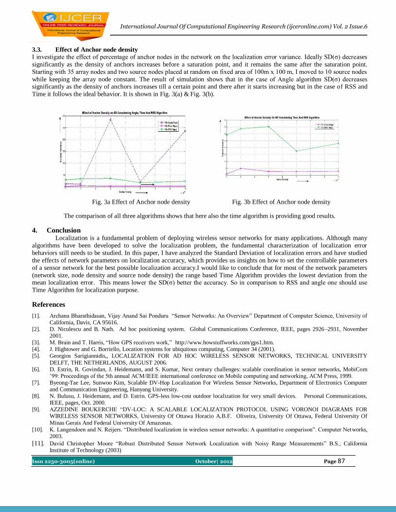
International Journal Of Computational Engineering Research (ijceronline.com) Vol. 2 Issue.6
Issn 2250-3005(online) October| 2012 Page 87
3.3. Effect of Anchor node density
I investigate the effect of percentage of anchor nodes in the network on the localization error variance. Ideally SD(σ) decreases
significantly as the density of anchors increases before a saturation point, and it remains the same after the saturation point.
Starting with 35 array nodes and two source nodes placed at random on fixed area of 100m ҳ 100 m, I moved to 10 source nodes
while keeping the array node constant. The result of simulation shows that in the case of Angle algorithm SD(σ) decreases significantly as the density of anchors increases till a certain point and there after it starts increasing but in the case of RSS and
Time it follows the ideal behavior. It is shown in Fig. 3(a) & Fig. 3(b).
Fig. 3a Effect of Anchor node density Fig. 3b Effect of Anchor node density
The comparison of all three algorithms shows that here also the time algorithm is providing good results.
4. Conclusion Localization is a fundamental problem of deploying wireless sensor networks for many applications. Although many
algorithms have been developed to solve the localization problem, the fundamental characterization of localization error
behaviors still needs to be studied. In this paper, I have analyzed the Standard Deviation of localization errors and have studied
the effects of network parameters on localization accuracy, which provides us insights on how to set the controllable parameters
of a sensor network for the best possible localization accuracy.I would like to conclude that for most of the network parameters
(network size, node density and source node density) the range based Time Algorithm provides the lowest deviation from the mean localization error. This means lower the SD(σ) better the accuracy. So in comparison to RSS and angle one should use
Time Algorithm for localization purpose.
References
[1]. Archana Bharathidasan, Vijay Anand Sai Ponduru “Sensor Networks: An Overview” Department of Computer Science, University of California, Davis, CA 95616.
[2]. D. Niculescu and B. Nath. Ad hoc positioning system. Global Communications Conference, IEEE, pages 2926–2931, November 2001.
[3]. M. Brain and T. Harris, “How GPS receivers work,” http://www.howstuffworks.com/gps1.htm. [4]. J. Hightower and G. Borriello, Location systems for ubiquitous computing, Computer 34 (2001). [5]. Georgios Sarigiannidis,, LOCALIZATION FOR AD HOC WIRELESS SENSOR NETWORKS, TECHNICAL UNIVERSITY
DELFT, THE NETHERLANDS, AUGUST 2006. [6]. D. Estrin, R. Govindan, J. Heidemann, and S. Kumar, Next century challenges: scalable coordination in sensor networks, MobiCom
’99: Proceedings of the 5th annual ACM/IEEE international conference on Mobile computing and networking, ACM Press, 1999. [7]. Byeong-Tae Lee, Sunwoo Kim, Scalable DV-Hop Localization For Wireless Sensor Networks, Department of Electronics Computer
and Communication Engineering, Hanyang University. [8]. N. Bulusu, J. Heidemann, and D. Estrin. GPS-less low-cost outdoor localization for very small devices. Personal Communications,
IEEE, pages, Oct. 2000. [9]. AZZEDINE BOUKERCHE “DV-LOC: A SCALABLE LOCALIZATION PROTOCOL USING VORONOI DIAGRAMS FOR
WIRELESS SENSOR NETWORKS, University Of Ottawa Horacio A.B.F. Oliveira, University Of Ottawa, Federal University Of
Minas Gerais And Federal University Of Amazonas. [10]. K. Langendoen and N. Reijers. “Distributed localization in wireless sensor networks: A quantitative comparison”. Computer Networks,
2003.
[11]. David Christopher Moore “Robust Distributed Sensor Network Localization with Noisy Range Measurements” B.S., California Institute of Technology (2003)

International Journal Of Computational Engineering Research (ijceronline.com) Vol. 2 Issue. 6
Issn 2250-3005(online) October| 2012 Page 88
Material Modeling Of Reactive Powder Concrete Using Ansys – A
Review.
Mr. M K Maroliya Assistant professor, Applied Mechanics Dept, Faculty of Technology & Engineering,
M.S. University of Baroda, Vadodara,
Abstract ANSYS has many finite element analysis capabilities, ranging from a simple, linear, static analysis to a complex,
nonlinear, transient dynamic analysis, which is used by engineers worldwide in virtually all fields of engineering. In order to
investigate the possibilities of current FE programs for implementation of steel fibre concrete this study was conducted. The
aim of this study was to show the use of steel fibre concrete with FE calculations, to point out the possibilities and restrictions
and to give recommendations for practical usage. Because of the complexities associated with the development of
rational analytical procedures, present day methods continue in many respect to be based on the empirical
approaches using result from a large amount of experimental data. The finite element (FE) method offers a powerful
and generic tool for studying the behavior of structures. Key words: RPC, non linear analysis, ANSYS, shear
1. Introduction In the emerging world of technologies, research on the concrete of better and better physical, mechanical and
durability, have given us much denser and ductile material called “Reactive Powder Concrete” (RPC). RPC is a special
concrete having ultra high strength and ductility. It is a cementitious composite where the micro structure is optimized by
precise gradation of all particles in the mix to yield maximum density. The design method for steel fibre reinforced concrete
(SFRC) recommended by RILEM TC 162-TDF is based on the traditional section-analysis method used for normal
reinforced concrete (RC) and, hence, offers a convenient means for designing SFRC elements. The difference between the
two design methods is that the stress-strain (σ-ε) model used for the design of SFRC does not ignore tension and takes into
account the tension stiffening due to the steel fibers.
The FE analyses of the RPC specimens tested in this investigation was carried out in using software ANSYS and procedure
to analyze structure using ANSYS.
2. Why Ansys? One of the main tasks for material engineers and structural designers who deal with quasibrittleBuilding materials is
the determination of fracture parameters. Usually these parameters are calculated from experimentally obtained data (load-
deflection diagram, l-d diagram) using Fracture-mechanics principles with the presumption that a stress concentrator formed
in theTesting specimen is a crack. ANSYS provides all the power of nonlinear structural capabilities as well as linear
capabilities to deliver the highest quality, most-reliable structural simulation results available. ANSYS post processing is
used to review the results once the solution has been calculated. There are two post processors general postprocessor and time
history postprocessor. The general postprocessor is used to obtain the contour displays, deformed shapes, and tabular listings
to review and interpret the results of the analysis. the graph plot of results data versus time and tabular listings can be
obtained from the time history postprocessor.
3. APPLICATION OF ANSYS IN STRUCTURAL ENGINEERING
Static analysis-A static analysis calculates the effects of steady loading conditions on a structure, while ignoring
inertia and damping effects, such as those caused by time-varying loads. A static analysis can, however, include steady inertia
loads (such as gravity and rotational velocity), and time varying loads that can be approximated as static equivalent loads
(such as the static equivalent wind and seismic loads commonly defined in many building codes). Modal analysis-Used to
calculate the natural frequencies and mode shapes of a structure. Different mode extraction methods are available.Transient
dynamic analysis- Used to determine the response of a structure to arbitrarily time-varying loads. All nonlinearities
mentioned under Static Analysis above are allowed.

International Journal Of Computational Engineering Research (ijceronline.com) Vol. 2 Issue. 6
Issn 2250-3005(online) October| 2012 Page 89
Spectrum analysis- An extension of the modal analysis, used to calculate stresses and strains due to a response spectrum or a
PSD input (random vibrations).Buckling analysis-Used to calculate the buckling loads and determine the buckling mode
shape. Both linear (eigenvalue) buckling and nonlinear buckling analyses are possible.
Fig.1.0 Flow diagram for analysis
Fig. 2.0 specimen meshing and stress contour
4. Modelling Modeling is the primary task of any analytical study and the result obtained to a large extent depends on the
simplification taken during in this step. Modeling involves creation of geometry of overall structure by including elements of
various components representing respective structural behavior including boundary conditions in the considered problem,
Material properties of various elements and loads on various elements and its combinations were defined.
ANSYS post processing is used to review the results once the solution has been calculated. There are two post processors
general postprocessor and time history postprocessor. The general postprocessor is used to obtain the contour displays,
deformed shapes, and tabular listings to review and interpret the results of the analysis. The graph plot of results data versus
time and tabular listings can be obtained from the time history postprocessor.

International Journal Of Computational Engineering Research (ijceronline.com) Vol. 2 Issue. 6
Issn 2250-3005(online) October| 2012 Page 90
4.0 RESULTS AND DISCUSSION
To the presence of dominant shear stresses, the specimen geometry was studied using finite element analysis, the
stress concentration are obtained as shown in Fig.2.0 indicating the possibility of cracking. The shear stress distribution is
shown in Fig. 2.0 with darker zone indicating higher stresses. It can be seen as that there is a zone of shear stresses at the
junction of “L” shape specimen, conforming that shear failure would occur if tensile cracking was to be restrained by fibres.
As a result clear shear crack propagation can be observed at the junction of “L” shape specimen.This paper presents a model
for determining the stress-strain characteristics of SFRC by using experimental data and FE analysis. This model describes
the behavior of SFRC in four phases and gives good results for a range of fibres tested. Optimum thickness of shear plane to
be considered is 60 mm which is getting conformed by FE analysis. Initially RPC shows linearly elastic behavior and then
dominated by plastic behavior representing the behavior of Elasto-plastic material. The toughening observed in the test is a
result of the pull out and dowel action of the fibre during the shear cracking. The pull out resistance tends to close the cracks,
while the shear forces tends to open it due to the irregularity of the crack face as illustrated in Fig.3.0 this produces a
confining effect which together with the dowel action of the fibres and friction between the crack faces, can lead to an
increase in the shear strength.
REFERENCES
1) Concrete Membrane Elements in Shear”. ACI Structural Journal, Vol.92, No. 6, pp. 1-15.
2) Yen lei Voo, Stephen j. Foster and R. Ian Gilbert (2006) “Shear Strength Of Fiber Reinforced Reactive Powder Concrete
Prestressed Girders Without Stirrups”. Journal of Advanced Concrete Technology Vol. 4, No. 1, pp. 123-132.
3) Russel, H G (1999) "ACI defines High -performance concrete", Concrete International, Vol. 21, pp. 56-57
4) Richard Pierre, Marcel Cheyrezy (1995) “Composition of Reactive Powder Concretes”. Cement and Concrete Research,
Vol. 25. no. 7, pp. 1501-1511
5) Oliver Bonneau, Claude Poulin, Jerome Dugat, P, Richard, and Pierre-Claude Aitcin (1999) “Reactive Powder
Concretes: From Theory to Practice”. Concrete International. pp.47-49.
6) Khaloo Ali R. and Nakeseok kim. (1997) “Influnce Of Concrete And Fibre Characteristics On Behavior Of Steel Fibre
Reinforced Concrete Under Direct Shear”. ACI Materials Journal, Vol. 94, No. 6, pp. 592-664.
7) Kazunori Fujikake, Takanori Senga, Nobuhito Ueda, Tomonori Ohno and Makoto Katagiri. (2006) “Nonlinear Analysis
For Reactive Powder Concrete Beam Under Rapid Flexural Loadings”. Journal of Advanced Concrete Technology Vol.
4, No. 1, pp. 85-97.
8) Francesco Bencardino; Lidia Rizzuti; Giuseppe Spadea; and Ramnath N. Swamy (2008) “Stress-Strain Behavior of Steel
Fiber-Reinforced Concrete in Compression” Journal of Materials in Civil Engg. ASCE, Vol 20 No. [3] pp. 255-263.
9) Chau K.T., X.X. Wei (2007) “Finite Solid Circular Cylinders Subjected To Arbitrary Surface Load. Part I – Analytic
Solution”. International Journal of Solids and Structures 37, pp. 5707-5732.
10) Chau K.T., X.X. Wei (2007) “Finite Solid Circular Cylinders Subjected To Arbitrary Surface Load. Part I – Analytic
Solution”. International Journal of Solids and Structures 37, pp. 5707-5732.
11) Bairagi N. K. and Modhera C. D. (2001) “Shear Strength Of Fibre Reinforced Concrete”. ICI Journal, Vol. 1, No. 4, pp.
47-52.
12) Abouzar Sadrekarimi. (2004) “Development of a Light Weight Reactive Powder Concrete”. Journal of Advanced
Concrete Technology Vol. 2, no. 3, pp. 409-417.
13) Byung-Wan Jo, Chang-Hyun Kim, (2007) "Characteristics Of Cement Mortar With Nano-Sio2 Particles", construction
and building Materials 21 pp. 1351-1355.
14) Chakraborti A.K., I. Ray, B.Sengupta (2001) “High Performance Concrete for Containment Structures”. Transactions
SMiRT 16, Washington DC, August 2001, pp.1-8.
15) Dias, WPS, et al, (1990). “Mechanical Proprieties Of Hardened Cement Paste Exposed To Temperature Up To 700°C
(1292°F)”. ACI Material Journal, 87(2): pp. 60 - 165.

International Journal Of Computational Engineering Research (ijceronline.com) Vol. 2 Issue. 6
Issn 2250-3005(online) October| 2012 Page 91
A Genetic Programming Approach for Detection of Diabetes
Prof. M. A. Pradhan1, Dr. G.R. Bamnote
2, Vinit Tribhuvan
3, Kiran Jadhav
4
Vijay Chabukswar5, Vijay Dhobale
6
1Asst. Prof., Department of Computer Engineering, AISSMS‘s College of Engineering, Pune, Maharashtra, India. 2 Asso. Prof., Department of Computer Engineering, PRMIT & R, Amrawati, Maharashtra, India.
3,4,5,6 Department of Computer Engineering, AISSMS‘s College of Engineering, Pune, Maharashtra, India.
Abstract: Diabetes is a malfunctioning of the body caused due to the deficiency of insulin & has now-a-days gained popularity,
globally. Although doctors diagnose diabetes using a blood glucose test, we cannot clearly classify the person as diabetic or not
based on these symptoms. Also a pre-diabetic phase can alert the doctors and the patient about the depreciating health and can
aware the patient about the concerned measures. In this paper, we propose a multi-class genetic programming (GP) based
classifier design that will help the medical practitioner to confirm his/her diagnosis towards pre-diabetic, diabetic and non-
diabetic patients.
Keywords: Classifier, Multi Class, Genetic Programming, GP, Diabetes Detection, Pre-diabetic.
1. Introduction Diabetes has now-a-days gained global popularity. The 21
st century with its sedentary lifestyle in the suburbs and a
fast, social, urban lifestyle all endanger an individual‘s life and promote him towards diabetes. Diabetes is a malfunctioning of
the body to produce insulin. Insulin is a hormone that helps the cells of the body take in sugar, or glucose, that is circulating in
the blood stream and use it for energy. The American Diabetes Association estimates that 25.8 million children and adults in
the United States—8.3% of the population—have diabetes and 7.0 million people are still undiagnosed[14]. Doctors diagnose
diabetes using a blood glucose test. A blood sample is drawn and the concentration of sugar in the plasma of the blood is
analyzed in a lab. Diagnosis of diabetes depends on many other factors and hence makes the medical practitioners job difficult,
at times. One high blood sugar test is not always enough to diagnose someone with diabetes especially if the person has no
other symptoms. Also, many a times it is noticed that in extreme cases, the doctor has also to depend upon his previous
knowledge and experience to diagnose the patient. Many a times, doctors prefer a second opinion too. Bearing all factors in
mind, a tool which enables the doctors to look at previous patients with similar conditions is necessary. The most important
factors in diagnosis are data taken from the patients and an expert‘s opinion. This is a primary reason for the growth of artificial
intelligence systems growing in health care industry [2]. Also a pre-diabetic phase can alert the doctors and the patient about the
depreciating health and can aware the patient about the concerned measures. In this paper, we propose a multi-class genetic
programming (GP) based classifier that will help the medical practitioner to confirm his/her diagnosis towards pre-diabetic,
diabetic and non-diabetic patients.
2. Related Work GP has already been used by a lot of authors to classify 2-class problems [3]–[8]. Karegowda et al. used neural
networks and presented a hybrid model which uses Genetic Algorithms (GA) and Back Propagation Network (BPN) for
classification of diabetes among PIMA Indians[18]. Polatet et al. proposed two different approaches for diabetes data
classification - principal component analysis and neuro-fuzzy inference and Generalized Discriminant Analysis (GDA) and
least square support vector machine (LS-SVM).They achieved an accuracy of 89.47% and 79.16% respectively[15][17]. Muni,
Pal, Das [22] proposed a method for multiclass classifier and introduced a new concept of unfitness for improving genetic
evolution. Hasan Temurtas et al.[16] proposed a neural approach for classification of diabetes data and achieved 82.37%
accuracy. Pradhan et al. used Comparative Partner Selection (CPS) along with GP to design a 2-class classifier for detecting
diabetes[17]. Cheung used C4.5, Naive Bayes, BNND and BNNF algorithms and reached the classification accuracies 81.11%,
81.48%, 81.11% and 80.96%, respectively[20]. Ephzibah [19] used a fuzzy rule based classification system for feature subset
selection in diabetes diagnosis. This approach proves to be cost-effective. Arcanjo et al. proposed a KNN-GP (KGP) algorithm,
a semi-supervised transductive one, based on the three basic assumptions of semi-supervised learning. This system was
implemented on 8 datasets of UCI repository but inferior results were obtained for diabetes dataset[21]. Having a look at multi-
class classifiers, a few researchers [9] - [12], have had an attempt with it. Kishore et al. [9] proposed an interesting method
which considers a class problem as a set of two-class problems[22]. Smart investigated the multi class approach using modified
genetic operators and concluded that GP can be used to improve multi class problems [24]. Lim et al. presented an excellent
comparison of 33 classification algorithms in [23]. They used a large number of benchmark data sets for comparison. None of
these 33 algorithms use GP [22].

International Journal Of Computational Engineering Research (ijceronline.com) Vol. 2 Issue. 6
Issn 2250-3005(online) October| 2012 Page 92
3. Introduction to GP The field of evolutionary computation (EC) has a variety of alternate methods and approaches to problem solving.
Some important approaches that have been applied to problems based on Genetic Algorithms (GA) classifier systems,
evolutionary strategies and evolutionary programming. Both GP and GA are being used for image feature extraction, selection,
and classifiers optimization. However, in recent years the field of Genetic Programming (GP) [1] has emerged as an effective
means for evolving solutions to problems. GP can represent solution in the form of computer programs.
Genetic Programming utilizes similar characteristics with GAs in the fundamental processes of evolution and natural
selection in order to construct solutions to problems. However, unlike GAs which use fixed sized binary strings, GPs use a
variable sized tree structure. An initial population of individuals is generated and tested against the problem at hand. An
objective fitness value is assigned to individuals based upon their ability to solve the problem, and then fitness proportionate
selection is used to select which individuals will pass their genetic material into the next generation using genetic operators like
crossover, mutation, and reproduction operations. An example of a GP tree has been shown in the figure below.
3.1. GP Operators
3.1.1. Crossover
In crossover (or recombination), two programs are selected from the population, both are then copied to a mating pool. A
crossover point is randomly chosen in each program, and the subtrees below the crossover points are swapped. The two
programs, with swapped subtrees, are then copied to the new population. This is pictured in the figure below.
3.1.2. Mutation
In mutation, a single program is selected from the population and copied to a mating pool. A mutation point is chosen
randomly, somewhere in the program, and the subtree below the mutation point is replaced with a new, randomly generated
subtree. The new program is then copied into the new population. This is pictured in figure below.
3.1.3. Reproduction
To ensure that the fitness of programs in a population is never less than that of previous generations, the reproduction, or
elitism, operator is used. This consists of simply copying the best few programs of a generation‘s population directly to the
next.

International Journal Of Computational Engineering Research (ijceronline.com) Vol. 2 Issue. 6
Issn 2250-3005(online) October| 2012 Page 93
3.2. Selection in GP Evaluation
The selection process determines which individual should be passed to next generation. Fitness value is the selection key of the
individuals. However, a number of methods help us to select the individuals based on the fitness values. The two primary
methods used in GP are described below.
3.2.1. Roulette-wheel selection: In this method a roulette wheel is broken into a number of segments. Each program in the
population takes one segment, but the size of each segment is relative to the fitness value of the program in the segment. The
fittest programs take larger segments while less fit programs take smaller sections. The roulette-wheel is spun many times to
select which individuals will be chosen for crossover, mutation, and reproduction operations. Every program has a chance of
being selected multiple times, but the probability of more fit programs being selected is greater due to the larger segment of the
wheel.
3.2.2. Tournament selection: Normally the selection of individuals is carried out over the entire population space; but in
tournament selection, competition for selection is divided into a large number of localized competitions, called tournaments. In
each tournament selection, a number of individuals between two and ten are selected at random from the population. The
individuals within the tournament then compete for a chance to be selected to pass genetic material into the next generation.
Usually only the best one or two individuals in the tournament, depending on tournament size, are selected. Each individual
program compete in several tournaments, but those programs with higher fitness values would have a better chance to win more
tournaments as compared to lower fitness.
3.3. Basic Terms of GP
3.3.1. Function Pool
It is a set of functions that will be used by the intermediate nodes in the structure of the tree. The function pool can contain
different types of functions which are problem dependent. All these functions may have different number of inputs but always
have a single output e.g. for logical problems logical functions like AND, OR, etc. are used. The function pool[2] that will be
used is +, -, *, /, square, √, sin, cos, asin, acos, log, abs, reciprocal.
3.3.2. Fitness Function
The most significant concept of genetic programming is the fitness function. Genetic Programming can solve a number of
problems; it is the fitness function which connects GP to the given problem. Each individual is assigned a fitness value by this
function. It determines how well a solution is able to solve the problem. It varies greatly from one type of the problem to
another. It is chosen in such a way that highly fitted solutions have high fitness value. Fitness function is the only index to
select a chromosome to reproduce for the next generation.
4. Proposed System
Genetic Programming uses Evolutionary Computation and trains computational programs to take human-like
decisions. In our proposed system, we consider Genetic Programming to evaluate and classify diabetic patients, based on the
previous knowledge imparted into the system. In association with Data Mining, Genetic Programming has been used to classify
a patient as pre-diabetic, diabetic or non-diabetic. This system not only provides a multiclass classifier of diabetes, but will also
act as a second opinion to doctors and medical practitioners. The ‗to-be diabetic‘ patients can also be warned and alerted and
necessary steps can be taken by the doctor towards them. This will help us to save important time in concern with the patients.
As the field of fuzzy systems and logical behaviour is rapidly growing, this multiclass GP approach can efficiently co-ordinate
doctors, especially the ones with no or little experience, to take major diagnostic decisions. Evolutionary Computation
techniques deal with enhancing optimization, as fuzzy systems with imprecision. These soft computing methodologies are
complementary and although a cent percent accuracy is not expected, convincing results for a multiclass (pre-diabetic, diabetic,
non-diabetic) classifier are promised, as multiclass classifiers are still in search of better and quicker results. Also a real time
dataset of diabetes is to be used, which will differentiate the system from the previous diabetes classifiers which used the PIMA
Indians dataset.
5. Conclusion We have proposed a GP approach to design classifiers for diabetes detection. It evolves an optimal classifier for a
multiclass problem i.e, pre-diabetic, diabetic, and non diabetic. The proposed system promises to evaluate quicker and better
results than those discussed in the current paper.

International Journal Of Computational Engineering Research (ijceronline.com) Vol. 2 Issue. 6
Issn 2250-3005(online) October| 2012 Page 94
References [1] J. R. Koza, Genetic Programming: On the Programming of Computers by Means of Natural Selection. Cambridge, MA:
MIT Press, 1992.
[2] M.W. Aslam, A.K. Nandi, ―Detection Of Diabetes Using Genetic Programming,‖ 18th European Signal Processing
Conference(EUSIPCO-2010),Aalborg, Denmark, August 2010.
[3] P. J. Rauss, J. M. Daida, and S. Chaudhary, ―Classification of spectral imagery using genetic programming,‖ in Proc.
Genetic Evolutionary Computation Conf., 2000, pp. 733–726.
[4] D. Agnelli, A. Bollini, and L. Lombardi, ―Image classification: an evolutionary approach,‖ Pattern Recognit. Lett., vol.
23, pp. 303–309, 2002.
[5] S. A. Stanhope and J. M. Daida, ―Genetic programming for automatic target classification and recognition in synthetic
aperture radar imagery,‖ in Evolutionary Programming VII, 1998, Proc. 7th Annu. Conf. Evolutionary Programming, pp.
735–744.
[6] I. De Falco, A. Della Cioppa, and E. Tarantino, ―Discovering interesting classification rules with genetic programming,‖
Appl. Soft Comput., vol.23, pp. 1–13, 2002.
[7] G. Dounias, A. Tsakonas, J. Jantzen, H. Axer, B. Bjerregaard, and D.Keyserlingk, ―Genetic programming for the
generation of crisp and fuzzy rule bases in classification and diagnosis of medical data,‖ in Proc. 1st Int. NAISO Congr.
Neuro Fuzzy Technologies, Canada, 2002, Academic Press, [CD-ROM].
[8] C. C. Bojarczuk, H. S. Lopes, and A. A. Freitas, ―Genetic Programming for knowledge discovery in chest pain
diagnosis,‖ IEEE Eng.Med. Mag.,vol. 19, no. 4, pp. 38–44, 2000.
[9] J. K. Kishore, L. M. Patnaik, V. Mani, and V. K. Agrawal, ―Application of genetic programming for multicategory
pattern classification,‖ IEEE Trans. Evol. Comput., vol. 4, pp. 242–258, Sept. 2000.
[10] T. Loveard and V. Ciesielski, ―Representing classification problems in genetic programming,‖ in Proc. Congr.
Evolutionary Computation,May 27–30, 2001, pp. 1070–1077.
[11] B.-C. Chien, J. Y. Lin, and T.-P. Hong, ―Learning discriminant functions with fuzzy attributes for classification using
genetic programming,‖ Expert Syst. Applicat., vol. 23, pp. 31–37, 2002.
[12] R. R. F. Mendes, F. B.Voznika, A. A. Freitas, and J. C. Nievola, ―Discovering fuzzy classification rules with genetic
programming and co-evolution,‖ in Lecture Notes in Artificial Intelligence, vol. 2168, Proc. 5th
Eur. Conf. PKDD, 2001,
pp. 314–325.
[13] R. Poli, ―Genetic Programming for image analysis,‖ in Proc. 1st Int.Conf. Genetic Programming, Stanford, CA, July
1996, pp. 363–368.
[14] American Diabetes Association http://www.diabetes.org/diabetes-statistics
[15] K. Polat, S. Gunes, A. Aslan, "A cascade learning system forclassification of diabetes disease: Generalized discriminant
analysis andleast square support vector machine", Expert systems with applications, vol.34(1), 2008, pp. 214-221.
[16] T. Hasan, Y. Nijat, T. Feyzullah, "A comparative study on diabetes disease using neural networks", Expert system with
applications, vol.36, May 2009, pp.8610-8615.
[17] M. A. Pradhan, Abdul Rahman, Pushkar Acharya, Ravindra Gawade, Ashish Pateria ―Design of Classifier for Detection
of Diabetes using Genetic Programming‖ , International Conference on Computer Science and Information Technology
(ICCSIT'2011) Pattaya Dec. 2011 , pp.125-130.
[18] Asha Gowda Karegowda , A.S. Manjunath , M.A. Jayaram ―APPLICATION OF GENETIC ALGORITHM
OPTIMIZED NEURAL NETWORK CONNECTION WEIGHTS FOR MEDICAL DIAGNOSIS OF PIMA INDIANS
DIABETES‖ , International Journal on Soft Computing ( IJSC ), Vol.2, No.2, May 2011, pp. 15-23.
[19] E.P.Ephzibah, ―COST EFFECTIVE APPROACH ON FEATURE SELECTION USING GENETIC ALGORITHMS
AND FUZZY LOGIC FOR DIABETES DIAGNOSIS.‖ , International Journal on Soft Computing ( IJSC ), Vol.2, No.1,
February 2011, pp. 1-10.
[20] Kemal Polata, & Salih Güne¸sa & Sülayman Tosunb, (2007), Diagnosis of heart disease using artificial immune
recognition system and fuzzy weighted pre-processing, ELSEVIER,PATTERN RECOGNATION.
[21] Filipe de L. Arcanjo, Gisele L. Pappa, Paulo V. Bicalho, Wagner Meira Jr., Altigran S. da Silva, ―Semi-supervised
Genetic Programming for Classification‖, GECCO’11, July 12–16, 2011, Dublin, Ireland.
[22] Durga Prasad Muni, Nikhil R. Pal, and Jyotirmoy Das, ―A Novel Approach to Design Classifiers Using Genetic
Programming‖, IEEE TRANSACTIONS ON EVOLUTIONARY COMPUTATION, VOL. 8, NO. 2, APRIL 2004, pp.
183-196.
[23] T.-S. Lim, W.-Y. Loh, and Y.-S. Shih, ―A comparison of prediction accuracy, complexity and training time of thirty-
three old and new classification algorithms,‖ Mach. Learning J., vol. 40, pp. 203–228, 2000.
[24] William Richmond Smart, ―Genetic Programming for Multiclass Object Classification‖, A thesis submitted to the
Victoria University of Wellington, 2005.

International Journal Of Computational Engineering Research (ijceronline.com) Vol. 2 Issue. 6
Issn 2250-3005(online) October| 2012 Page 95
An Improved Heuristic for Permutation Flow Shop Scheduling
(NEH ALGORITHM) 1Ekta Singhal,
2Shalu Singh,
3Aneesh Dayma
(Department of Software Engineering), 3 (Department of Computer Science), Suresh Gyan Vihar University,Jaipur
Abstract- Flowshop Scheduling is used to determine the optimal sequence of n jobs to be processed on m machines
in the same order. Permutation Flowshop Scheduling
Problems (PFSP) require same job sequence on all the
machines with the constraint that machines can only process
one job at a time and jobs can be processed by only one
machine at a time. No machine is allowed to remain idle
when a job is ready for processing. Such problems are NP-
Complete and hence optimal solutions are not guaranteed
but heuristics have been shown to produce good working solutions.
NEH (Nawaz, Enscore, Ham) Algorithm is an
efficient algorithm that works by minimizing the makespan
for Permutation Flowshop Scheduling Problems PFSP. The
proposed algorithm is obtained by modifying the NEH
algorithm and produces improved quality solutions with
algorithmic complexity same as the original algorithm.
Keywords: Flowshop Scheduling, heuristics, makespan
I. Introduction 1.1 Important Definitions
1.1.1 Heuristics
Heuristic refers to experience-based techniques for problem
solving, learning, and discovery. Heuristic methods are used
to speed up the process of finding a good enough solution,
where an exhaustive search is impractical[6].
1.1.2 Flowshop Scheduling
Flowshop Scheduling determines an optimum sequence of n
jobs to be processed on m machines in the same order i.e.
every job must be processed on machines 1,2,...,m in this
same order[10].
1.1.3 Permutation Flowshop Scheduling
Permutation Flowshop Scheduling is a special case of FSPs
where same job sequence is followed in all machines i.e.
processing order of the jobs on the machines is the same for
every machine.
1.1.4 NP-Complete A problem L is NP-complete if it has two properties:
It is in the set of NP (nondeterministic polynomial time) problems: Any given solution to L can be verified
quickly (in polynomial time).
It is also in the set of NP-hard problems: Any NP
problem can be converted into L by a transformation of the
inputs in polynomial time. Although any given solution to
such a problem can be verified quickly, there is no known
efficient way to locate a solution in the first place; indeed,
the most notable characteristic of NP-complete problems is
that no fast solution to them is known. That is, the time
required to solve the problem using any currently known
algorithm increases very quickly as the size of the problem grows.
1.1.5 Makespan
Makespan is the completion time of last job on last
machine.
1.1.6 Constructive Heuristics
In constructive heuristics once a decision is taken it cannot
be changed for improvement[10].
1.1.7 Improvement Heuristics
Pawel J. Kalczynski, Jerzy Kamburowski [3] used
improvement heuristics, we start with an initial sequence
and attempt to improve it as we proceed.
1.2 Problem Definition
The permutation flow shop problem requires to find the
order in which n jobs are to be processed on m consecutive
machines. The jobs are processed in the order machine 1,
machine 2, . . . machine m.
Machines can only process one job at a time and jobs can
be processed by only one machine at a time without
preemption.
No job can jump over any other job, meaning that the order
in which jobs are processed in machine 1 is maintained throughout the system. Moreover, no machine is allowed to
remain idle when a job is ready for processing. All jobs and
machines are available at time 0.
II. OBJECTIVE For each job two parameters are computed:
tp (i, j) processing time of job j on machine i
tc (i, j) completion time of job j on machine i

International Journal Of Computational Engineering Research (ijceronline.com) Vol. 2 Issue. 6
Issn 2250-3005(online) October| 2012 Page 96
The completion time of all jobs is can be computed as:
tc (M1, J1) = tp (M1, J1)
tc (Mi, J1) = tc (Mi-1, J1) + tp (Mi, J1)
tc (M1, Jj) = tc (M1, Jj-1) + tp (M1, Jj)
tc (Mi, Jj) = max tc (Mi-1, Jj), tc (Mi, Jj-1) + tp (Mi, Jj)
The objective is to find an n-job sequence so as to minimize
the makespan i.e. tc (Mm, Jn).
III. Neh Algorithm (Nawaz Enscore Ham)
It is a constructive heuristic.
Step 1: Sort the n jobs in non-increasing order of their total
processing times
Step 2: Take the first two jobs and schedule them in order to
minimise the partial makespan as if there were only these
two jobs
Step 3: For k= 3 to n do Step 4
Step 4: Insert the kth job at the place, which minimises the
partial makespan among the k possible ones.
IV. Improved Heuristic Step 1: Sort the n jobs in non-increasing order of their total
processing times
Step 2: Take the first four jobs from the sorted list and form
4! = 24 partial sequences (each of length 4). The best k (k is
a parameter of the algorithm) out of these 24 partial
sequences are selected for further processing. The relative
positions of jobs in any partial sequence is not altered in any
later (larger) sequence
Step 3: Set z = 5
Step 4: The zth job on the sorted list is inserted at each of
the z positions in each of the k (z − 1)-job partial sequences, resulting in (z × k) z-job partial sequences
Step 5: The best k out of the z × k sequences are selected for
further processing
Step 6: Increment z by 1
Step 7: If z > n, accept the best of the k n-job sequences as
the final solution and stop.
Otherwise go to step 4.
V. Comparision (EXAMPLE)
Comparison (Example)
Machin
e 1
Machin
e 2
Machin
e 3
Machin
e 4
Machin
e 5
Job 1
(J1)
5 9 8 10 1
Job 2
(J2)
9 3 10 1 8
Job 3
(J3)
9 4 5 8 6
Job 4
(J4)
4 8 8 7 2
Job 5
(J5)
3 5 6 3 7
Total processing times of jobs
Job 1= 5+9+8+10+1= 33
Job 2= 9+3+10+1+8= 31 Job 3= 9+4+5+8+6= 32
Job 4= 4+8+8+7+2= 29
Job 5= 3+5+6+3+7= 24
Sorting in non-increasing order of total processing times
J1, J3, J2, J4, J5
NEH Algorithm
Fig: 1
Fig: 2

International Journal Of Computational Engineering Research (ijceronline.com) Vol. 2 Issue. 6
Issn 2250-3005(online) October| 2012 Page 97
Sequence: J1-J3 Makespan: 46
Sequence: J3-J1 Makespan: 42
Select sequence J3-J1
Fig: 3
Fig: 4
Fig: 5
Sequence: J2-J3-J1 Makespan: 51
Sequence: J3-J2-J1 Makespan: 51
Sequence: J3-J1-J2 Makespan: 50
Select sequence J3-J1-J2
Fig: 6
Fig: 7
Fig: 8
Fig: 9
Sequence: J4-J3-J1-J2 Makespan: 54
Sequence: J3-J4-J1-J2 Makespan: 57
Sequence: J3-J1-J4-J2 Makespan: 58
Sequence: J3-J1-J2-J4 Makespan: 58
Select sequence J4-J3-J1-J2

International Journal Of Computational Engineering Research (ijceronline.com) Vol. 2 Issue. 6
Issn 2250-3005(online) October| 2012 Page 98
Fig: 10
Fig: 11
Fig: 12
Fig: 13
Fig: 14
Sequence:
J5- J4-J3-J1-J2
Makespan: 58
Sequence: J4-
J5- J3-J1-J2 Makespan: 58
Sequence: J4-
J3- J5-J1-J2
Makespan: 59
Sequence: J4-J3-J1-J5-J2 Makespan: 63 Sequence: J4-J3-J1-J2-J5 Makespan: 61
Thus, the best sequence is J5-J4-J3-J2-J1 and J4-J5-J3-J1-
J2 with makespan of 58.
VI. Improved Heuristic
Taking first four jobs from the sorted order to form 24
partial sequences.
Sequence: J1-J2-J3-J4 Makespan: 59 Sequence: J1-J4-J2-J3 Makespan: 59
Sequence: J1-J3-J2-J4 Makespan: 57
Sequence: J1-J4-J3-J2 Makespan: 61
Sequence: J3-J1-J2-J4 Makespan: 58
Sequence: J3-J4-J1-J2 Makespan: 57
Sequence: J2-J1-J3-J4 Makespan: 58
Sequence: J2-J4-J1-J3 Makespan: 62
Sequence: J2-J3-J1-J4 Makespan: 58
Sequence: J2-J4-J3-J1 Makespan: 56
Sequence: J3-J2-J1-J4 Makespan: 58
Sequence: J3-J4-J2-J1 Makespan: 58 Sequence: J1-J2-J4-J3 Makespan: 61
Sequence: J4-J1-J2-J3 Makespan: 58
Sequence: J1-J3-J4-J2 Makespan: 58
Sequence: J4-J1-J3-J2 Makespan: 63
Sequence: J3-J1-J4-J2 Makespan: 58
Sequence: J4-J3-J1-J2 Makespan: 54
Sequence: J2-J1-J4-J3 Makespan: 62
Sequence: J4-J2-J1-J3 Makespan: 63
Sequence: J3-J2-J4-J1 Makespan: 58
Sequence: J4-J3-J2-J1 Makespan: 55
Sequence: J4-J2-J3-J1 Makespan: 55 Sequence: J2-J3-J4-J1 Makespan: 57

International Journal Of Computational Engineering Research (ijceronline.com) Vol. 2 Issue. 6
Issn 2250-3005(online) October| 2012 Page 99
The parameter of the algorithm k is taken as 7.
Selecting the best 7 sequences for further processing.
J4-J3-J1-J2
Sequence: J5-J4-J3-J1-J2 Makespan: 58
Sequence: J4-J5-J3-J1-J2 Makespan: 58
Sequence: J4-J3-J5-J1-J2 Makespan: 59
Sequence: J4-J3-J1-J5-J2 Makespan: 63
Sequence: J4-J3-J1-J2-J5 Makespan: 61
J4-J3-J2-J1
Sequence: J5-J4-J3-J2-J1 Makespan: 58
Sequence: J4-J5-J3-J2-J1 Makespan: 60
Sequence: J4-J3-J5-J2-J1 Makespan: 60
Sequence: J4-J3-J2-J5-J1 Makespan: 60
Sequence: J4-J3-J2-J1-J5 Makespan: 64
J4-J2-J3-J1
Sequence: J5-J4-J2-J3-J1 Makespan: 58
Sequence: J4-J5-J2-J3-J1 Makespan: 60
Sequence: J4-J2-J5-J3-J1 Makespan: 60 Sequence: J4-J2-J3-J5-J1 Makespan: 60
Sequence: J4-J2-J3-J1-J5 Makespan: 64
J2-J4-J3-J1
Sequence: J5-J2-J4-J3-J1 Makespan: 60
Sequence: J2-J5-J4-J3-J1 Makespan: 62
Sequence: J2-J4-J5-J3-J1 Makespan: 60
Sequence: J2-J4-J3-J5-J1 Makespan: 60
Sequence: J2-J4-J3-J1-J5 Makespan: 65
J2-J3-J4-J1 Sequence: J5-J2-J3-J4-J1 Makespan: 62
Sequence: J2-J5-J3-J4-J1 Makespan: 61
Sequence: J2-J3-J5-J4-J1 Makespan: 63
Sequence: J2-J3-J4-J5-J1 Makespan: 63
Sequence: J2-J3-J4-J1-J5 Makespan: 67
J1-J3-J2-J4
Sequence: J5-J1-J3-J2-J4 Makespan: 59
Sequence: J1-J5-J3-J2-J4 Makespan: 60
Sequence: J1-J3-J5-J2-J4 Makespan: 63
Sequence: J1-J3-J2-J5-J4 Makespan: 63
Sequence: J1-J3-J2-J4-J5 Makespan: 63
J3-J4-J1-J2
Sequence: J5-J3-J4-J1-J2 Makespan: 60
Sequence: J3-J5-J4-J1-J2 Makespan: 62
Sequence: J3-J4-J5-J1-J2 Makespan: 62
Sequence: J3-J4-J1-J5-J2 Makespan: 66
Sequence: J3-J4-J1-J2-J5 Makespan: 64
Thus, the best sequences are
J5-J4-J3-J1-J2
J4-J5-J3-J1-J2
J5-J4-J3-J2-J1
J5-J4-J2-J3-J1
with makespan of 58.
VII. Complexity Complexity of NEH Algorithm The total number of enumerations in Neh is given by
n(n+1)/2
which clearly states that the complexity of this algorithm is
Θ(n^2).
Complexity of improved heuristic
The total number of enumerations in case of the improved
heuristic is given by[18]
4! + ∑, (z=5 to n) k * z
= 4! + k * ∑, (z=5 to n) z
Where, k denotes the algorithm parameter,
And n is the number of jobs.
Hence, the algorithmic complexity of this approach is Θ(n^2).
VIII. Conclusions The improved heuristic proposed for PFSP yields better
result than original NEH algorithm while maintaining the
same algorithmic complexity.
As shown using an example, the improved heuristic
generates more number of minimum makespan sequences as
compared to the NEH algorithm and hence we have more options of job sequences that can be implemented for
greater production.
Experimental studies show that the improved heuristic for
PFSP results in sequences with lower makespan as
compared to those obtained from NEH algorithm in case of
medium sized (n=12 – 30) and large sized (n>70) problems.
IX. Future Scope NEH is considered to be the best known heuristic for PFSPs. But the proposed heuristic has been proved to
outperform NEH.
Hence, this heuristic has a great scope in industry where n
jobs are required to be scheduled on m machines for greater
production, efficient planning of resources and maintaining
proper control over the industry.

International Journal Of Computational Engineering Research (ijceronline.com) Vol. 2 Issue. 6
Issn 2250-3005(online) October| 2012 Page 100
References [1] Dipak Laha , Uday Kumar Chakraborty, (2007), Int.
J. Information and Communication Technology,
Vol. 1, No. 1
[2] Nawaz, M., Enscore Jr, E. and Ham, I., (91-95), The
International Journal of Management Science. v11.
91-95. [3] Pawel J. Kalczynski, Jerzy Kamburowski, (2008),
Journal Computers and Operations Research,
Volume 35, Issue9
[4] Bestwick, P.F. and Hastings, N.A.J. (1976) ‘A new
bound for machine scheduling’, Operational
Research Quarterly, Vol. 27, pp.479–490.
[5] Brown, A.P.G. and Lomnicki, Z.A. (1966) ‘Some
applications of the branch and bound algorithm to
the machine scheduling problem’, Operational
Research Quarterly, Vol. 17, pp.173–182.
[6] Campbell, H.G., Dudek, R.A. and Smith, M.L.
(1970) ‘A heuristic algorithm for the n-job, m-machine sequencing problem’, Management
Science, Vol. 16, pp.630–637.
[7] Cormen, T.H., Leiserson, C.E. and Rivest, R.L.
(1990) ‘Introduction to Algorithms’,
Cambridge,MA: MIT Press.
[8] Dannenbring, D.G. (1977) ‘An evaluation of
flowshop sequencing heuristics’, Management
Science,Vol. 23, No. 11, pp.1174–1182.
[9] Gupta, J.N.D. (1971) ‘A functional heuristic
algorithm for the flow-shop scheduling
problem’,Operational Research Quaterly, Vol. 22, No. 1.
[10] Ignall, E. and Schrage, L. (1965) ‘Application of the
branch-and-bound technique to some flowshop
scheduling problems’, Operations Research, Vol.
13, pp.400–412.
[11] Johnson, S.M. (1954) ‘Two and three stage
production schedules with set-up times included’,
Naval Research Logistics Quarterly, Vol. 1, pp.61–
68.
[12] Koulamas, C. (1998) ‘A new constructive heuristic
for the flowshop scheduling problem’, European
Journal of Operations Research, Vol. 105, pp.66–71. [13] Kreyszig, E. (1972) ‘Advanced Engineering
Mathematics’, New York: John Wiley.
[14] Lomnicki, Z.A. (1965) ‘A branch-and-bound
algorithm for the exact solution of the three-machine
scheduling problem’, Operational Research
Quarterly, Vol. 16, pp.89–100.
[15] Nawaz, M., Enscore Jr., E.E. and Ham, I. (1983) ‘A
heuristic algorithm for the m-machine n-job
flowshop sequencing problem’, OMEGA
International Journal of Management Science,
Vol. 11, pp.91–95.
[16] Palmer, D.S. (1965) ‘Sequencing jobs through a
multi-stage process in the minimum total time - a
quick method of obtaining a near-optimum’,
Operational Research Quarterly, Vol. 16, No. 1,
pp.101–107.
[17] Sarin, S. and Lefoka, M. (1993) ‘Scheduling
heuristics for the n-job, m-machine flowshop’,
OMEGA,Vol. 21, pp.229–234.
[18] Turner, S. and Booth, D. (1987) ‘Comparison of
heuristics for flowshop sequencing’, OMEGA,Vol. 15,pp.75–78

International Journal Of Computational Engineering Research (ijceronline.com) Vol. 2 Issue. 6
Issn 2250-3005(online) October| 2012 Page 101
Triple Connected Two Domination Number of a Graph
G. Mahadevan1 Selvam Avadayappan
2 B. Ayisha
3 T. Subramanian
4
1,4Dept. of Mathematics, Anna University : Tirunelveli Region, Tirunelveli.
2Dept.of Mathematics, VHNSN College, Virudhunagar.
3Research Scholar, Manonmaniam Sundaranar University, Tirunelveli.
Abstract: The concept of triple connected graphs with real life application was introduced in [7] by considering the
existence of a path containing any three vertices of a graph G. In[3], G. Mahadevan et. al., was introduced the concept of
triple connected domination number of a graph. In this paper, we introduce a new domination parameter, called triple
connected two domination number of a graph. A subset S of V of a nontrivial graph G is called a dominating set of G if
every vertex in V − S is adjacent to at least one vertex in S. The domination number (G) of G is the minimum cardinality
taken over all dominating sets in G. A subset S of V of a nontrivial graph G is said to be triple connected dominating set, if
S is a dominating set and the induced sub graph <S> is triple connected. The minimum cardinality taken over all triple
connected dominating sets is called the triple connected domination number and is denoted by tc. A dominating set is
said to be two dominating set if every vertex in V – S is adjacent to atleast two vertices in S. The minimum cardinality
taken over all two dominating sets is called the two domination number and is denoted by 2. A subset S of V of a
nontrivial graph G is said to be triple connected two dominating set, if S is a two dominating set and the induced sub
graph <S> is triple connected. The minimum cardinality taken over all triple connected two dominating sets is called the
triple connected two domination number and is denoted by 2tc. We determine this number for some standard graphs and
obtain bounds for general graph. Its relationship with other graph theoretical parameters are also investigated.
Key words: Domination Number, Triple connected graph, Triple connected domination number, Triple connected two
domination number.
AMS (2010): 05C69
1. Introduction By a graph we mean a finite, simple, connected and undirected graph G(V, E), where V denotes its vertex set
and E its edge set. Unless otherwise stated, the graph G has p vertices and q edges. Degree of a vertex v is denoted by
d(v), the maximum degree of a graph G is denoted by Δ(G). We denote a cycle on p vertices by Cp, a path on p vertices by
Pp, and a complete graph on p vertices by Kp. A graph G is connected if any two vertices of G are connected by a path. A
maximal connected subgraph of a graph G is called a component of G. The number of components of G is denoted by
(G). The complement of G is the graph with vertex set V in which two vertices are adjacent if and only if they are not
adjacent in G. A tree is a connected acyclic graph. A bipartite graph (or bigraph) is a graph whose vertex set can be
divided into two disjoint sets V1 and V2 such that every edge has one end in V1 and another end in V2. A complete bipartite
graph is a bipartite graph where every vertex of V1 is adjacent to every vertex in V2. The complete bipartite graph with
partitions of order |V1|=m and |V2|=n, is denoted by Km,n. A star, denoted by K1,p-1 is a tree with one root vertex and p – 1
pendant vertices. The open neighbourhood of a set S of vertices of a graph G, denoted by N(S) is the set of all vertices
adjacent to some vertex in S and N(S) S is called the closed neighbourhood of S, denoted by N[S]. A cut – vertex (cut
edge) of a graph G is a vertex (edge) whose removal increases the number of components. A vertex cut, or separating set
of a connected graph G is a set of vertices whose removal results in a disconnected. The connectivity or vertex
connectivity of a graph G, denoted by κ(G) (where G is not complete) is the size of a smallest vertex cut. A connected
subgraph H of a connected graph G is called a H -cut if (G – H) ≥ 2. The chromatic number of a graph G, denoted by
χ(G) is the smallest number of colors needed to colour all the vertices of a graph G in which adjacent vertices receive
different colours. For any real number , denotes the largest integer less than or equal to . A Nordhaus -Gaddum-
type result is a (tight) lower or upper bound on the sum or product of a parameter of a graph and its complement. Terms
not defined here are used in the sense of [2]. A subset S of V is called a dominating set of G if every vertex in V − S is
adjacent to at least one vertex in S. The domination number (G) of G is the minimum cardinality taken over all
dominating sets in G. A dominating set S of a connected graph G is said to be a connected dominating set of G if the
induced sub graph <S> is connected. The minimum cardinality taken over all connected dominating sets is the connected
domination number and is denoted by c.A dominating set is said to be two dominating set if every vertex in V – S is
adjacent to atleast two vertices in S. The minimum cardinality taken over all two dominating sets is called the two
domination number and is denoted by 2.Many authors have introduced different types of domination parameters by
imposing conditions on the dominating set [8, 9]. Recently, the concept of triple connected graphs has been introduced by
Paulraj Joseph J. et. al.,[7] by considering the existence of a path containing any three vertices of G. They have studied the

International Journal Of Computational Engineering Research (ijceronline.com) Vol. 2 Issue. 6
Issn 2250-3005(online) October| 2012 Page 102
properties of triple connected graphs and established many results on them. A graph G is said to be triple connected if any
three vertices lie on a path in G. All paths, cycles, complete graphs and wheels are some standard examples of triple
connected graphs.In[3], G. Mahadevan et. al., was introduced the concept of triple connected domination number of a
graph. A subset S of V of a nontrivial graph G is said to be a triple connected dominating set, if S is a dominating set and
the induced subgraph <S> is triple connected. The minimum cardinality taken over all triple connected dominating sets is
called the triple connected domination number of G and is denoted by tc(G). Any triple connected dominating set with
tc vertices is called a tc -set of G. In[4, 5, 6] G. Mahadevan et. al., was introduced complementary triple connected
domination number, complementary perfect triple connected domination number and paired triple connected
domination number of a graph and investigated new results on them.
In this paper, we use this idea to develop the concept of triple connected two dominating set and triple connected
two domination number of a graph.
Theorem 1.1 [7] A tree T is triple connected if and only if T Pp; p ≥ 3.
Theorem 1.2 [7] A connected graph G is not triple connected if and only if there exists a H -cut with (G – H) ≥ 3
such that = 1 for at least three components C1, C2, and C3 of G – H.
Notation 1.3 Let G be a connected graph with m vertices v1, v2, …., vm. The graph obtained from G by attaching n1 times a
pendant vertex of on the vertex v1, n2 times a pendant vertex of on the vertex v2 and so on, is denoted by G(n1 ,
n2 , n3 , …., nm ) where ni, li ≥ 0 and 1 ≤ i ≤ m.
Example 1.4 Let v1, v2, v3, v4, be the vertices of K4. The graph K4(P2, P3, 2P4, P3) is obtained from K4 by attaching 1 time
a pendant vertex of P2 on v1, 1 time a pendant vertex of P3 on v2, 2 times a pendant vertex of P4 on v3 and 1 time a pendant
vertex of P3 on v4 and is shown in Figure 1.1.
Figure 1.1 : K4(P2, P3, 2P4, P3)
2. Triple connected two domination number
Definition 2.1 A subset S of V of a nontrivial graph G is said to be a triple connected two dominating set, if S is a two
dominating set and the induced subgraph <S> is triple connected. The minimum cardinality taken over all triple
connected two dominating sets is called the triple connected two domination number of G and is denoted by 2tc(G). Any
triple connected two dominating set with 2tc vertices is called a 2tc -set of G.
Example 2.2 For the graph G1 in Figure 2.1, S = v1, v2, v3 forms a 2tc -set of G1. Hence 2tc(G1) = 3.
Figure 2.1 : Graph with 2tc = 3.
Observation 2.3 Triple connected two dominating set does not exists for all graphs and if exists, then 2tc(G) ≥ 3.
Example 2.4 For the graph G2 in Figure 2.2, any minimum two dominating set must contain the vertices v1, v4, v5. But
any two dominating set contains these vertices is not triple connected and hence 2tc does not exists.
Figure 2.2 : Graph with no tctd set
Throughout this paper we consider only connected graphs for which triple connected two dominating set exists.
Observation 2.5 The complement of the triple connected two dominating set need not be a triple connected two
dominating set.
Example 2.6 For the graph G3 in Figure 2.3, = v3, v4, v5 forms a triple connected two dominating set of G3. But the
complement V – S = v1, v2, v6 is not a triple connected two dominating set.
v5
G1: v1
v4
v3 v2
v6 v7
G3:
v3 v1 v2
v4 v5 v6
v1
v3 v4
v2

International Journal Of Computational Engineering Research (ijceronline.com) Vol. 2 Issue. 6
Issn 2250-3005(online) October| 2012 Page 103
Figure 2.3 : Graph in which V – S is not a tctd set
Observation 2.7 Every triple connected two dominating set is a dominating set but not conversely.
Theorem 2.8 If the induced subgraph of each connected dominating set of G has more than two pendant vertices, then G
does not contain a triple connected two dominating set.
Proof The proof follows from Theorem 1.2.
Exact value for some standard graphs:
1) For any cycle of order p ≥ 4, 2tc(Cp) = p – 1.
2) For any complete graph of order p ≥ 4, 2tc(Kp) = 3.
3) For any complete bipartite graph of order p ≥ 4, 2tc(Km,n) = 3.
(where m, n ≥ 2 and m + n = p ).
Observation 2.9 If a spanning sub graph H of a graph G has a triple connected two dominating set, then G also has a
triple connected two dominating set.
Observation 2.10 Let G be a connected graph and H be a spanning sub graph of G. If H has a triple connected two
dominating set, then 2tc(G) ≤ 2tc(H) and the bound is sharp.
Example 2.11 Consider the graph G4 and its spanning subgraph H4 and G5 and its spanning subgraph H5 shown in Figure
2.4.
Figure 2.4
For the graph G4, S = v1, v2, v4 is a triple connected two dominating set and so 2tc(G4) = 3. For the spanning
subgraph H4 of G4, S = v1, v3, u4, v2 is a triple connected two dominating set so that 2tc(H4) = 4. Hence 2tc(G4)
< 2tc(H4). For the graph G5, S = v1, v5, v4 is a triple connected two dominating set and so 2tc(G5) = 3. For the spanning
subgraph H5 of G5, S = v1, v5, v4 is a triple connected two dominating set so that 2tc(H5) = 3.Hence 2tc(G5) = 2tc(H5).
Theorem 2.12 For any connected graph G with p ≥ 4, we have 3 2tc(G) ≤ p – 1 and the bounds are sharp.
Proof The lower and bounds follows from Definition 2.1. For K4, the lower bound is attained and for C5 the upper bound
is attained.
Observation 2.13 For any connected graph G with 4 vertices, 2tc(G) = p – 1 if and only if G K4, W4, C4, C3(P2),
K4 – e.
Theorem 2.14 For any connected graph G with 5 vertices, 2tc(G) = p – 1 if and only if G C5, C4(P2), C3(P3),
C3(P2, P2, 0) or the graph G6 shown in Figure 2.5 .
Figure 2.5 Proof Suppose G is isomorphic to C5, C4(P2), C3(P3), C3(P2, P2, 0) or the graph G6 given in Figure 2.5, then clearly
2tc(G) = p – 1. Conversely, Let G be a connected graph with 5 vertices, and 2tc(G) = 4. Let S = v1, v2, v3, v4 be the
2tc(G) -set of G. Hence <S> = P4, C4, C3(P2), K4 – e.
G3: v3
v1 v2
v4 v5
v6
G4:
v1
v5
v2
v3 v4
H4:
v1
v5
v2
v3 v4
G5: v5
v3 v4
v1 v2
H5: v5
v3 v4
v1 v2
G6:
v5
v3 v4 v1 v2

International Journal Of Computational Engineering Research (ijceronline.com) Vol. 2 Issue. 6
Issn 2250-3005(online) October| 2012 Page 104
Case(i): Let <S> = P4 = v1v2v3v4. Since S is a triple connected two dominating set, v5 is adjacent to atleast two vertices of
S. If v5 is adjacent to v1 and v2, then G C3(P3). If v5 is adjacent to v1 and v3, then G C4(P2). If v5 is adjacent to v1 and
v4, then G C5. If v5 is adjacent to v2 and v3, then G C3(P2, P2, 0). If v5 is adjacent to v1, v2 and v3, then G G6.
Case(ii): Let <S> = C4 = v1v2v3v4v1.
Since S is a triple connected two dominating set, v5 is adjacent to atleast two vertices of S. Either if v5 is adjacent
to v1 and v2 or v1 and v3, we can find a triple connected dominating set with less than four vertices, which is a
contradiction.
Case(iii): Let <S> = C3(P2).
Let v1v2v3v1 be the cycle and v4 be adjacent to v1. Since S is a triple connected two dominating set, v5 is adjacent
to atleast two vertices of S. For all the possibilities of v5 is adjacent to two vertices of S, we can find a triple connected
dominating set with less than four vertices, which is a contradiction.
Case(iv): Let <S> = K4 – e. Since S is a triple connected two dominating set, v5 is adjacent to atleast two vertices of S.
For all the possibilities of v5 is adjacent to two vertices of S, we can find a triple connected dominating set with less than
four vertices, which is a contradiction.
The Nordhaus – Gaddum type result is given below:
Theorem 2.15 Let G be a graph such that G and have no isolates of order p ≥ 4. Then
(i) 2tc(G) + 2tc( ) ≤ 2p – 2.
(ii) 2tc(G). 2tc( ) ≤ (p – 1)2 and the bound is sharp.
Proof The bound directly follows from Theorem 2.12. For path C4, both the bounds are attained.
3 Relation with Other Graph Theoretical Parameters
Theorem 3.1 For any connected graph G with p ≥ 4 vertices, 2tc(G) + κ(G) ≤ 2p – 2 and the bound is sharp if and only if
G K4.
Proof Let G be a connected graph with p ≥ 4 vertices. We know that κ(G) ≤ p – 1 and by Theorem 2.12, 2tc(G) ≤ p – 1.
Hence 2tc(G) + κ(G) ≤ 2p – 2. Suppose G is isomorphic to K4. Then clearly 2tc(G) + κ(G) = 2p – 2. Conversely, Let
2tc(G) + κ(G) = 2p – 2. This is possible only if 2tc(G) = p – 1 and κ(G) = p – 1. But κ(G) = p – 1, and so G Kp for
which 2tc(G) = 3 = p – 1. Hence G K4.
Theorem 3.2 For any connected graph G with p ≥ 4 vertices, 2tc(G) + (G) ≤ 2p – 1 and the bound is sharp if and only if
G K4.
Proof Let G be a connected graph with p ≥ 4 vertices. We know that (G) ≤ p and by Theorem 2.12, 2tc(G) ≤ p – 1.
Hence 2tc(G) + (G) ≤ 2p – 1. Suppose G is isomorphic to K4. Then clearly 2tc(G) + (G) = 2p – 1. Conversely, let
2tc(G) + (G) = 2p – 1. This is possible only if 2tc(G) = p – 1 and (G) = p. Since (G) = p, G is isomorphic to Kp for
which 2tc(G) = 3 = p – 1. Hence G K4.
Theorem 3.3 For any connected graph G with p ≥ 4 vertices, 2tc(G) + (G) ≤ 2p – 2 and the bound is sharp.
Proof Let G be a connected graph with p ≥ 4 vertices. We know that (G) ≤ p – 1 and by Theorem 2.12, 2tc(G) ≤ p – 1.
Hence 2tc(G) + (G) ≤ 2p – 2. For K4, the bound is sharp.
REFERENCES
[1] Cokayne E. J. and Hedetniemi S. T. (1980): Total domination in graphs, Networks, Vol.10: 211–219.
[2] John Adrian Bondy, Murty U.S.R. (2009): Graph Theory, Springer, 2008.
[3] Mahadevan G., Selvam A., Paulraj Joseph J., and Subramanian T. (2012): Triple connected domination number of a
graph, IJMC, Vol.3.
[4] Mahadevan G., Selvam A., Paulraj Joseph J., Ayisha B., and Subramanian T. (2012): Complementary triple connected
domination number of a graph , Accepted for publication in Advances and Applications in Discrete Mathematics, ISSN 0974-
1658.
[5] Mahadevan G, Selvam Avadayappan, Mydeen bibi A., Subramanian T. (2012): Complementary perfect triple connected
domination number of a graph, International Journal of Engineering Research and Application, ISSN 2248- 9622, Vol.2, Issue
5, Sep – Oct, pp 260-265.
[6] Mahadevan. G, Selvam Avadayappan, Nagarajan. A, Rajeswari. A, Subramanian. T. (2012): Paired Triple connected
domination number of a graph, International Journal of Computational Engineering Research, Vol. 2, Issue 5, Sep., pp. 1333-
1338.
[7] Paulraj Joseph J., Angel Jebitha M.K., Chithra Devi P. and Sudhana G. (2012): Triple connected graphs, Indian Journal of
Mathematics and Mathematical Sciences, ISSN 0973-3329 Vol. 8, No. 1, pp. 61-75.
[8] Paulraj Joseph J. and Mahadevan G. (2006): On complementary perfect domination number of a graph, Acta Ciencia
Indica, Vol. XXXI M, No. 2.: 847–853.
[9] Teresa W. Haynes, Stephen T. Hedetniemi and Peter J. Slater (1998): Domination in graphs, Advanced Topics, Marcel Dekker,
New York.
[10] Teresa W. Haynes, Stephen T. Hedetniemi and Peter J. Slater (1998): Fundamentals of domination in graphs, Marcel
Dekker, New York.

International Journal Of Computational Engineering Research (ijceronline.com) Vol. 2 Issue. 6
Issn 2250-3005(online) October| 2012 Page 105
Feasibility study of a roof top Solar room heater
Tejinder Kumar Jindal Assistant Professor
Aerospace Engineering Department
PEC University of Technology Chandigarh
Abstract: The present work describes a low cost solar space heater. The device is the replacement of the concrete cantilevers
used above the windows in houses facing the south direction. An experiment was conducting by making a suitable device for
use for the purpose. It has been observed that the device can be used to heat the space for the south facing room windows
directly and for the other directions by circulating the air through the device kept at the roof top making an angle of about 38
degree with the roof top.
Key words: duct, draught, heat transfer, rooftop, solar collector, solar chimney, ventilation.
1. Introduction With the exponential growth of energy demand, efforts are being made all over the world to conserve energy. As non-
renewable sources are consumed, the mankind must turn its attention to longer-term, permanent type of energy sources. Solar
energy one of the abundant source promise of becoming a dependable energy because it is environmentally clean source of
energy and available free of cost. Solar energy has been identified as one of the promising alternative energy source for the
future.
On average the extraterrestrial irradiance is 1367 W/m2, which is also known as Solar Constant. Total power from the
sun intercepted by the earth is approximately 1.8 X 10¹¹
MW, which is many thousand of times larger than the present
consumption rate on earth. In addition to its size, solar energy can be used in a decentralized manner, reducing the cost of
transmission and distribution of power.
There are two distinct methods for converting solar energy to work: thermodynamic conversion and direct conversion.
In thermodynamic conversion, solar collectors first convert solar energy to heat. This heat is then partially converted to work
in accordance with second law of thermodynamics. There is a well defined theoretical upper limit to the efficiency of any
process that converts heat to work. Efficiencies of direct conversion processes are not limited by second law of
thermodynamics, but they have their own practical limitations.
There are some problems associated with the use of solar energy. The main problem is that it is a dilute source of
energy. Even in the hottest regions on earth, the solar radiation flux available rarely exceeds 1 KW/m2 and total radiation
over a day is best about 7 KW/m2. These are low values from the point of view of technological utilization. Consequently
large collecting areas are required in many applications and these results in excessive costs.
The major technical obstacle for solar thermal application is the intermittent nature of the source, both on daily and
short time scale. The intermittent nature leads to a storage requirement, generally not present in non solar systems. The extra
cost and complexity of storage is a negative point to solar systems. Solar systems also require a good solar climate for
efficient operation. This is favorable in case of India: land for solar collector is abundant and where energy demand is high,
the solar flux is also high and direct beam component maximum. Finally, solar system must meet the criteria of economic
competitiveness in order to be widely accepted. On the other hand, solar energy has an advantageous position compared with
scarce fossil fuels. Most of the energy demands in India (and elsewhere also) can be met by simple solar systems. There are
very few new components like collectors, controls which are complex. By proper application of solar techniques, an excellent
thermodynamic match between the solar energy resources and many end-uses can be achieved.
2. Solar Chimney Like natural draught chimney, solar chimney is a vertical tubular structure of transparent material, steel, reinforced
concrete or reinforced plastic built for the purpose of enclosing a column of hot air heated by the solar collector. So, solar
chimney has one side (facing the sun) made of transparent material like glass to absorb solar energy. The draught produced
by the chimney is due to the density difference between the column of hot air inside the chimney and the cold air outside. The
efficiency of the chimney is directly proportional to the height of the chimney.There are mainly two applications of solar
chimneys[1,2].

International Journal Of Computational Engineering Research (ijceronline.com) Vol. 2 Issue. 6
Issn 2250-3005(online) October| 2012 Page 106
2.1 Ventilation in buildings
Ventilation is a widely used technique for removal of indoor contaminants as a measure of pollutant source control.
Natural ventilation is usually used in regions with mild climates and in spaces where some variation in indoor climate is
tolerable. A solar chimney is a good configuration to implement natural ventilation in buildings where solar energy is
available. It is similar to a conventional chimney except that the south wall is replaced by glazing, which enables solar energy
collection. The flow caused is directly influenced by the pressure distribution on the building envelope and the characteristics
of the different openings. The pressure distribution is the driving force for ventilation while the characteristics of each
opening, among other things, determine the flow resistance[3,4].
2.2 Solar Chimney Turbine
Solar Chimney Turbine utilizes the airflow inside the chimney to run a turbine. The turbine being coupled to a
generator produces electric power. Turbines are always placed at the base of the chimney. Using turbines, mechanical output
in the form of rotational energy can be derived from the air current in the chimney. Turbines in a solar chimney do not work
with staged velocity as a free running wind energy converter, but as a cased pressure-staged wind turbo generator, in which
similar to a hydroelectric power station, static pressure is converted to rotational energy using a cased turbine.
There are large numbers of applications of solar energy, and even larger is the number of systems and their
components achieving the energy conversion goal. To maximize the efficiency of any complete system, the efficiencies of the
components must be maximized/optimized[5,6].
3. Roof Top Solar System The solar flat plate collector and the solar chimney concept have been integrated in the present study. An open flat
plate solar thermal collector has been fitted with a solar chimney to enhance the speed of the outgoing hot air through the
collector the temperature of the air is sufficient to heat the room. Small fan can be installed at the entry to the room for
smooth entry of the hot air.
4. Experimental setup An experimental setup was fabricated for the purpose of study the heating power of an about 1.5 m
2 flat plate
collector. The dimensional sizes for collector are 1700 mm X 850 mm X 115mm. The inclination of collector on the stand
iskept at 180, 28
0, 38
0 and
48
0 by suitably lifting the base of the stand. The collector-chimney assembly is supported by a steel
structure and can be tilted at different angles. The absorber plate is 0.6 mm thick GI sheet painted black. The bottom of the
collector is insulated using 5 cm thick glass wool. Thermal conductivity of glass wool is 0.04 W/m K. Two sidewalls are also
insulated by 6cm thick glass wool, with 12mm wooden backing. The top cover, the collector is 5mm thick window glass this
is in four pieces made airtight using adhesive and transparent cello tape. The properties of Glass and parameters of the setup
are as follows.
Thermal Conductivity 0.937 W/m K
Density (at 20º C) 2.44 g/cm³
Thermal Expansion 8.6 x 10 -6
/°C
Collector Area 1.445 m2
Chimney Exit Area 0.00866 m2
Hot air flow rate 0.01014 * V
Enthalpy change of air m Cp T
Where,
T Temperature difference
V Velocity of air in m/s is
The air temperature inside the channel was recorded by eleven k-type thermocouples. Six arranged at a spacing of
25cm along the centre line of the absorber plate along the airflow direction and five arranged in the chimney at spacing of
20cm. The distance from the channel inlet to these temperature measurement sections were 450, 700, 950, 1200, 1450, 1700,
1900, 2100, 2300, 2500 and 2700 mm, respectively. Atmospheric temperature noted made by k-type thermocouple, which is
portable with the display unit, this thermocouple is named thermocouple number 1.

International Journal Of Computational Engineering Research (ijceronline.com) Vol. 2 Issue. 6
Issn 2250-3005(online) October| 2012 Page 107
The velocity of air at outlet of the channel is measured by a vane type anemometer. For pressure measurement in the
chimney section static pressure ports were also provided and connected to water tube manometer. As there were not any
significant pressure changes in the system, so these ports were closed in the early experimentation stage.
Figure-1 Photo of the Experimental Setup
5. Results And Discussions Experiments were carried out at different inclination angles of the collector and at different times of the day. Various
angles taken were 180, 28
0, 38
0, 48
0 the collector. Measurements were made from 9:00 to 17:00h, at an interval of one hour.
The measured and calculated values of the parameters are shown in the following figures.
The most important is to study the effect of collector inclination on the performance of the system. Mass flow rate is
directly related with the power output of a solar chimney power plant, hence has been taken as the optimization criteria.
Second reason to choose mass flow rate as the controlling factor is due to the size and scale of the system. From a small
chimney height and 1.4 m2 collector area it is not possible to run a turbine and hence take turbine output as the criteria. Solar
radiation angle also affects the mass flow rate with inclination. For buoyant flow higher inclination angle causes higher stack
pressure for driving natural ventilation. However, under otherwise identical conditions, the convective heat transfer
coefficient inside the air channel decreases with the increase of inclination angle, which results in the reduction of natural
ventilation airflow rate.
Figure 5 shows that, initially, the natural ventilation air-flow rate enhances with the increase of inclination angle,
and then it reaches the peak value at about 380 inclination angle. Finally, it begins to fall off, which indicates that the decrease
of convection heat transfer overwhelms the increase of stack pressure after the inclination angle is beyond 380, the
phenomena being also governed by solar angles.
Figure-2. Mass Flow Rate v/s Time at 38
0 inclination

International Journal Of Computational Engineering Research (ijceronline.com) Vol. 2 Issue. 6
Issn 2250-3005(online) October| 2012 Page 108
0
10
20
30
40
50
60
70
80
450 700
9501200
14501700
19002100
23002500
2700
Distance (mm)
Tem
p (d
eg. C
elsi
us)
Temp
Figure-3 Temperature variation at Collector exit with Distance
Figure 4. Enthalpy Gain vs. Time at 38
0 inclination

International Journal Of Computational Engineering Research (ijceronline.com) Vol. 2 Issue. 6
Issn 2250-3005(online) October| 2012 Page 109
0
0.002
0.004
0.006
0.008
0.01
0.012
0.014
0.016
0.018
9:00
10:00
11:00
12:00
13:00
14:00
15:00
16:00
17:00
Time (hrs)
m (
Kg
/s)
18 deg 28 deg 38 deg 48 deg
Figure-5 Variation of Mass Flow Rate with Collector Inclination and time
The inclined collector Solar Chimney has the potential to increase the overall performance of Solar Chimney Power
Plant. The inclination of collector greatly affects the mass flow through the chimney, which was taken as the optimization
parameter. Hence collector ingle inclination should be opted for and must be optimized in solar induced flow inside a solar
chimney power plant. By Experimentation the optimum collector tilt angle for Chandigarh (May month) has been found to be
in the range 35-400. The average power comes out to be 300W. It can be enhanced to 1.5 KW by putting double glass
collector and increasing area to 2-3 m2. Hence it is clear that a solar chimney roof collector is feasible
References [1] Anthony J. Gannon, Theodor W. von Backstr Öm, ”The Solar Chimney Air Standard Cycle” R & D Journal (South
Africa) 2000.
[2] A.J. Gannon and T.W. von Backström, “Solar Chimney Turbine Performance” ASME Journal of Solar Energy
Engineering, February 2003, Vol. 125/101.
[3] J. Hirunlabh, W. Kongduang, P. Namprakai, J. Khedari “Study of natural ventilation of houses by a metallic solar wall
under tropical climate” Renewable Energy 18 (1999) 109-119.
[4] Joseph Khedari, Weerapong Mansirisub, Sompong Chaima, Naris Pratinthong, Jongjit Hirunlabh, “Field
measurements of performance of roof solar collector” Energy and Buildings 31 (2000),171–178.
[5] Joseph Khedari, Boonlert Boonsri, Jongjit Hirunlabh, “Ventilation impact of a solar chimney on indoor temperature
fluctuation and air change in a school building” Energy and Buildings 32 (2000) 89–93.
[6] M. M. Sanchez, M. Lucas, P. Martinez, A. Sanchez and A. Viedma, “Climatic Solar Roof: An Ecological Alternative
to Heat Dissipation in Buildings” Solar Energy Vol. 73, No. 6, pp. 419–432, 2002.

International Journal Of Computational Engineering Research (ijceronline.com) Vol. 2 Issue. 6
Issn 2250-3005(online) October| 2012 Page 110
Automatic Syllabification Rules for Bodo Language
Jyotismita Talukdar1 Chandan Sarma
2, Prof.P.H Talukdar
3
1Asian Institute of Technology, Gauhati University, India,
Abstract Syllabification performs the task of Identifying syllables in a word or in a sentence. Most of the syllabification tasks are done
manually. As the syllabification rules vary from language to language so it is difficult to design a common syllabification rules or
algorithm to fit all the languages. On the other hand Syllabification rules are the basic backbone for any task related to text-to-speech
conversion system. An attempt has been made through this paper to design an automatic syllabification rules for Bodo language . An
algorithm has been developed for automatic syllabification of Bodo language and the algorithm is evaluation on 5000 phonetically
rich words obtained from different sources like Text books, Newspapers and Radio News. The result is compared with the same
words manually syllabified. The algorithm performs well upto about 95.5 %
Key Words: Text-to speech, phoneme, syllable , monophthongs etc.
1. 0: INTRODUCTION A Syllable is a unit between phoneme and word. It is larger than phoneme and smaller than word[1]. Many theories are
available in phonetics and phonology to define a syllable [2]. In phonetics, the syllables are defined based upon the articulation [3].
But in phonology, the syllables are termed as the different sequences of the phonemes.
In Syllabification , a word is divided into its constituent syllables [4]. Syllabification is an important component in TTS
system [5]. It helps the implementation of certain letter-to-phoneme rules or Grapheme-to-Phoneme(G2P) rules. Detecting the
syllable correctly helps in modeling duration and improve the synthesized speech intonation. The syllabification has a big role in
enhancing the quality of synthetic speech. The quality of a TTS system is measured by the extent of naturalness of the synthetic speech
produced by the system [6]. Syllabification helps to improve the naturalness of the synthetic speech [7].
Text-to-speech (TTS) systems are considered as a very mature technology in the speech area [3]. It permits automatic
synthesis of speech from text. To make the systems more robust, efficient and reliable, it is crucial to have a good
Pre-processing module for the word corpus to be used in the training of a TTS system and for the texts to be synthesized. The
pre-processing module , also known as front-end, is composed of three stages: text analysis, phonetic analysis and prosodic
generation.
In this paper an algorithm to syllabify Bodo words into syllables is proposed. The algorithm was tested on a text corpus
which contains representative words for each grammatical rule. The degree of success was measured in terms of the percentage of
correctly syllabified words.
2.0: BODO LANGUAGE AND ITS PHONOLOGICAL STRUCTURE Bodo language belongs to the branch of Barish section under Baric division of the Tibeto-Burman languages. It is spoken by
the Bodo people of north-eastern India, part of North Bengal and Nepal. The language is one of the official languages of the Indian
state of Assam, and is one of the 22 scheduled languages . The inventory of Bodo phonemes consists of the number of (a) Segmental
phonemes being consonants and vowels and (b) Suprasegmental phonemes being tone, juncture and contour, co-occurring with
them as extra sound features used in the language [9]. Bodo language contains 22 segmental phonemes; six pure vowels or
monophthongs and sixteen consonants including two semi vowels.
The Bodo vowels and consonants are shown in Table 1.0 and Table2.0
Table 1.0: Bodo Vowels
Front Central Back
Close I u w
Mid E Ɔ
Open a
Table 2.0: Bodo Consonalts

International Journal Of Computational Engineering Research (ijceronline.com) Vol. 2 Issue. 6
Issn 2250-3005(online) October| 2012 Page 111
Manner
of articulation
Bilabia
l
Alveol
ar
Alveolo-
Palatal
Velar Glott
al
Vl V
d
Vl V
d
Vl Vd Vl Vd Vd
S T O P
b d g
ph t
h k
h
Nasal m n ŋ
Fricative s z h
Trill r
Lateral l
Semi-vowel w j
2. Syllabfication Phonological rules and constraints basically apply within syllables or at syllable boundaries , so the linguists view syllables
as an important unit of prosody [10]. Apart from purely linguistic significance, syllables play an important role in speech synthesis
and recognition [11]. For a given phoneme the pronunciation tends to vary depending on its location within a syllable. While actual
implementations vary, text-to-speech (TTS) systems must have, at minimum, three components [12] : a letter-to-phoneme (L2P)
module, a prosody module, and a synthesis module. Syllabification play important roles in all these three components.
3.1:Methodology
The methodology followed in the present study was (i) To examine the Bodo Syllable structures from the Linguistics
literature (ii) Gathering the opinions of scholars from the various linguistic traditions. (iii) Dialects variations. Based on these three
issues we have developed syllabification rules and an algorithm to syllabify Bodo words automatically.
3.2: Syllable Structure in Bodo.
Bodo language is highly monosyllabic. A Bodo word may be either a monosyllabic or a polysyllabic, co-occurring with
either rising tones or falling tones.
The syllables are described as sequences of phonemes in segments of the vowels(V) and the consonants(C) and also of the
clusters in consonants. The Bodo syllable structures may be divided into the following types based on the distribution of the segmental
phonemes and consonantal clusters-
1. V
2. VC
3. CCV
4. CCVC
5. CVCVCC
6. CVCCCVC
7. CVCCVCCVCCV
3.3:Syllabification Procedure
In Bodo language every syllable has at least one vowel sound. So, number of vowel sounds in a word equals to the number of
syllable. A monosyllabic word (e.g /ai/) need not to be syllabified and consonants blends and digraphs (/kh/, /ph/) also need not to be
syllabified. The basic rules of syllabification in Bodo are detailed below :.
1) A word with single vowel syllable boundary assigned at the end of the word.(Rule #1).
2) For vowels with different sounds in a word, the syllable boundary is marked after the first vowel.ie if VV then V/V. (Rule
#2).
3) For a word with consonant-vowel structure like VCV then mark the syllable boundary after the first vowel.ie if VCV then
V/CV. (Rule #3).
4) For a word with consonant-vowel structure like VCCV means two consonants exist between two vowels then mark the
syllable boundary between the consonants.ie if VCCV then VC/CV.(Rule #4).

International Journal Of Computational Engineering Research (ijceronline.com) Vol. 2 Issue. 6
Issn 2250-3005(online) October| 2012 Page 112
5) With three consonants comes between two vowels in a word like VCCCV then mark the syllable boundary after the first
consonants.ie if VCCCV then VC/CCV.(Rule #5)
6) Aa word with consonant-vowel structure like CVVC means two vowels come between two consonants then mark the
syllable boundary between the vowels forming two syllables.ie if CVVC then CV/VC.(Rule #6)
7) A word with consonant-vowel structure like CVVCV , mark the syllable boundary after two consecutive vowels.ie if
CVVCV then CVV/CV.(Rule #7).
8) If a word has consonant-vowel structure like VCVC or VCVV means VCV followed by either C or V then mark syllable
boundary after the first vowel.ie if VCVC or VCVV then V/CVC or V/CVV.(Rule #8).
9) If a word has consonant-vowel structure like CVCVV or CVCVC means CVC followed by either VV or VC then mark the
syllable boundary between first vowel and the consonant followed by it.ie if CVCVV or CVCVC then CV/CVV or CV/CVC.
(Rule# 9).
10) If a word has consonant-vowel structure like CVCCV means if CVC is followed by CV then mark the syllable boundary
between two consecutive consonants.ie if CVCCV then CVC/CV.(Rule #10) .
3.4 Syllabification Action
All the rules, as mentioned above, were implemented in the algorithm that executes as many iterations as possible to have all
the syllables of a given word separated. The Algorithm analyzed a word from left to right. On each iteration, the algorithm attempts to
find a new syllable in the portion of the word that has not yet been analyzed by trying to match one of the rules with this entire portion
or just part of it. The algorithm follow the hierarchical sequence for the verification of these rules defined above. When a rule is
matched, depending on its definition, the algorithm extracts a new syllable from that part of the word which is currently under analysis.
4.0: Syllabification Algorithm: In this section, the Bodo syllabification rules identified in the section (3.3) are presented in the form of a formal algorithm.
The function syllabify() accepts an array of phonemes generated, along with a variable called current_index which is used to
determine the position of the given array currently being processed by the algorithm.
Initially the current_index variable will be initialized to 0. The syllabify() functionis called recursively until all phonemes in
the array are processed. The function mark_syllable_boundary(position) will mark the syllable boundaries of an accepted array of
phonemes. The other functions used within the syllabify() function are described
below.
total_vowels(phonemes): accepts an array of phonemes and returns the number of vowels contained in that array.
is_vowel(phoneme): accepts a phoneme and returns true if the given phoneme is a vowel.
count_no_of_consonants_upto_next_vowel(phonemes, position): accepts an array of phonemes and a starting position; and
returns the count of consonants from the starting position of the given array until the next vowel is found.
The complete listing of the algorithm is as follows:
function syllabify (phonemes, current_index)
if total_vowels(phonemes) is 1 then
mark_syllable_boundary(at_the_end_of_phonemes)
else
if is_vowel(phonemes[current_index]) is true then
total_consonants=
count_no_of_consonants_upto_next_vowel
(phonemes,current_index)
if total_consonants is 0 then
if is_vowel(phonemes[current_index+1]) is true then

International Journal Of Computational Engineering Research (ijceronline.com) Vol. 2 Issue. 6
Issn 2250-3005(online) October| 2012 Page 113
if is_vowel(phonemes[current_index+3) is true
then
mark_syllable_boundary(current_index+1)
syllabify(phonemes,current_index+2)
end if
mark_syllable_boundary(current_index)
syllabify(phonemes, current_index+1)
end if
else
if total_consonants is 1 then
mark_syllable_boundary(current_index)
syllabify(phonemes, current_index + 2)
end if
if no_of_consonants are 2 then
mark_syllable_boundary(current_index+1)
syllabify(phonemes, current_index+3)
end if
if total_consonants are 3 then
mark_syllable_boundary(current_index+1)
syllabify(phonemes,current_index+4)
end if
end if
else
syllabify(phonemes,current_index+1)
end if
5.0: Results and Discussion The above algorithm was tested on 5000 distinct words extracted from a Bodo corpus and then compared with manual
syllabification of the same words to measure accuracy.
Heterogeneous nature of texts obtained from the News Paper, Feature Articles Text books, Radio news etc was chosen for
testing the algorithm due to. A list of distinct words was first extracted, and the 5000 most frequently occurring words chosen for
testing the algorithm.
The 5000 words yielded some 18,755 syllables .The algorithm achieves an overall accuracy of 97.05% when compared with
the same words manually syllabified by an expert.
An error analysis revealed that foreign words directly encoded in Bodo produces error.
6. Conclusion Syllabification is an important component of many speech and language processing systems, and this algorithm is expected
to be a significant contribution to the field, and especially to researchers working on various aspects of the Sinhala language.
REFERENCES
[1.] ChandanSarma,U.Sharma,C.K.Nath,S.Kalita,P.H.Taluk dar, Selection of Units and Development of Speech
[2.] Database for Natural Sounding Bodo TTS System, CISP Guwahati ,March 2012.
[3.] Parminder Singh, Gurpreet Singh Lehal, Syllables Selection for the Development of Speech Database for
[4.] Punjabi TTS System , IJCSI International Journal of Computer Science Issues, Vol. 7, Issue 6, November 2010.
[5.] R.A. Krakow, Physiological organization of syllables: a review, Journal of Phonetics, Vol. 27, 1999, pp. 23-54.
[6.] Susan Bartlett, Grzegorz Kondrak, Colin Cherry, On the Syllabification of Phonemes, Human Language
[7.] Technologies: The 2009 Annual Conference of the North American Chapter of the ACL, pages 308– 316,Boulder,
Colorado, June 2009. c 2009 Association for Computational Linguistics.
[8.] Y. A. El-Imam, Phonetization of arabic: rules and algorithms, Computer Speech & Language, vol. 18, pp. 339–373,
October 2004.
[9.] A.W. Black and K.A. Lenzo,Building synthetic voice, http://festvox.org/bsv/, 2003

International Journal Of Computational Engineering Research (ijceronline.com) Vol. 2 Issue. 6
Issn 2250-3005(online) October| 2012 Page 114
[10.] R. Dale et al. (Eds.), A Rule Based Syllabification Algorithm for Sinhala, IJCNLP 2005, LNAI 3651, pp. 438 – 449,
2005.© Springer-Verlag Berlin Heidelberg 2005.
[11.] Couto I., Neto N., Tadaiesky, V. Klautau, A. Maia, R.2010. An open source HMM-based text-to-speech
[12.] system for Brazilian Portuguese. Proc. 7th International Telecommunications Symposium Manaus.
[13.] Madhu Ram Baro, Structure of Boro language,2008
[14.] Juliette Blevins,The syllable in phonological theory,1995
[15.] George Kiraz and Bernd M¨obius, Multilingual syllabification using weighted finite-state transducers.In Proceedings
of the 3rd Workshop on Speech Synthesis,1998.
[16.] Robert Damper. 2001. Learning about speech from data: Beyond NETtalk. In Data-Driven Techniques in
[17.] Speech Synthesis, pages 1–25. Kluwer Academic Publishers.

International Journal Of Computational Engineering Research (ijceronline.com) Vol. 2 Issue. 6
Issn 2250-3005(online) October| 2012 Page 115
Promoter Recognition in human genome
Chandrashekar.Jatoth1, T. Shobha Rani
2
1 Computational Intelligence Lab, Department of Computer and Information Sciences, University of Hyderabad,
Hyderabad, India 2 Computational Intelligence Lab, Department of Computer and Information Sciences, University of Hyderabad,
Hyderabad, India
Abstract— promoter is a specific region of DNA that
facilitates the transcription of a particular gene. Promoters are typically located near the genes they regulate, on the same strand and upstream (towards the 5′ region of the sense strand). Promoters contain specific DNA sequences and response elements which provide binding sites for RNA polymerase and for proteins called transcription factors that recruit RNA polymerase. Promoter prediction programs (ppps) are computational models which aim at identifying the promoter regions in a genome. The
main approaches of the promoter prediction are either assigning scores to all single nucleotides to identify TSS or identifying a promoter region without providing scores to all nucleotides. In this project n-gram features are extracted and used in promoter prediction. Here a systematic study is made to discover the efficacy of n-grams (n=2, 3, 4, 5) as features in promoter prediction problem. Neural network classifiers with these n-grams as features are used to identify promoters in a human genome. In
this case for n=4 we are getting optimal values.
Keywords—Biological data sets, machine learning method,
neural networks, in silico method for promoter prediction, Binary classification, cascaded classifiers.
I. Introduction Promoter recognition is a real problem that computationally identifies the transcription start site (TSS) or the 5’end of the gene without time-consuming and expensive experimental methods that align ESTs, cDNAs or mRNAs against to the entire genome. In
this article, we focus on humans because it is a representative species that has attracted much more attention in the past decade. In humans, the TSS is surrounded with a core-promoter region within around ±100 base pairs (bp). A proximal promoter region has several hundreds bp immediately upstream of the core promoter. The capacity of transcription factors (TFs) to activate gene expression is encoded in both the core and proximal promoters, which are composed of short regulatory elements that
function as transcription factor binding sites (TFBSs) for specific TFs to control and regulate the transcription initiation of the gene. Therefore, the rich information encoded in promoters is crucial to locate the accurate position of the TSS. Figure1. Shows a schematic representation of the locations of the promoter region, TFBSs, TSS, 5’ UTR, exons, introns and 30 UTR. So far, high-resolution promoter recognition algorithms have at least two important motivations. First, they can improve the genome
annotation when the experimental support of ESTs, cDNAs or mRNAs is not available. Second, they can efficiently narrow down the regions in transcriptional regulation for inspiring further
Experimental work because the computational approach is much cheaper.
Figure 1: A schematic representation of the locations of the promoter
region, TFBSs, exons, introns and 3′utr regions.
Available promoter prediction systems use two types of features for classification namely, context features like nmers, and signal features such as TATA-box, CCAAT-box, and CpG islands. Among the favorable promoter prediction programs, Eponine [1]
builds a PWM to detect TATA-box and G+C enrichment regions as promoter-like regions; FirstEF [2] uses CpG-related and non-CpG related first exons as signal features; Promoter Inspector [3]
uses IUPAC words with wildcards as context features. Good experiment results are achieved by integrating these two types of features. DPF [4] applies a separate module on G+C rich and G+C poor regions, and selects 256 pentamers to generate a PWM for prediction. Furthermore, DragonGSF [5, 6] adds the CpG-island feature to DPF.
Most of the promoter prediction programs try to predict the exact location of the promoter region of the known protein-
coding genes, while some focus on finding the transcription start site (TSS). Some research has show that there is often no single TSS, but rather a whole transcription start region (TSR) containing multiple TSSs that are used with different frequencies. Generally two main approaches are used in promoter prediction [7].
1. First approach assigns scores to all single nucleotides to Identify TSS.
2. Second approach identifies a promoter region without providing scores for all nucleotides.
In this article analyzes the performance of 17 programs on two tasks: Genome wide identification of the start of genes and Genome wide identification of TSRs. In Existing methods Promoter prediction programs DragonGSF predicts the value of precision is between 37-48% and recall is 51-70%, DragonPF predicts the value of precision is between 61-65% and recall 62-
64%, FristEF predicts the value of precision is 79-81% and recall 35-40%, Eponine predicts the value of precision is ≈ 40 and recall ≈ 67%, NNPP2.2 predicts the value of precision is 69-93% and recall 2.0-4.5%, McPromoter2.0 predicts the value of precision is 26-57%and recall ≈ 4.5, proSom predicts the value of precision is 0.38% and recall 0.66% [8].

International Journal Of Computational Engineering Research (ijceronline.com) Vol. 2 Issue. 6
Issn 2250-3005(online) October| 2012 Page 116
We select the 13 representative PPPs that can analyze large
genome sequences and report strand-specific TSS predictions. ARTS, Eponine used SVM as the part of their design, EP3, Promoter scan, Wu-method used Position weight matrix (PWM). CpGcluster used distance based algorithm. CpGProD used linear discriminating analysis (LDA). DragonGSF, DragonPF, McPromoter used neural networks.NNPP2.2 has used Time Delay neural network. Promoter Explorer has used AbaBoost algorithm. proSOM has used SOM. These programs have used as features
various aspects of promoter and other regions of the DNA [6]. There are three classification methods for human promoter recognition system [9].
• Discriminative model that finds the optimal thresholds or classification boundaries in the signal, context and structure features space. Typical methods include artificial neural networks (ANNs), discriminate functions and support vector machines (SVMs).
• Generative model that describes the generative process of signal, context and structure observations. Position weight matrix (PWM), nearest neighborhood and hidden Markov models (HMMs) belong to generative models.
• Ensemble that combines multiple classifiers for multiple features in order to achieve a consensus and robust recognition results.
Promoter Inspector is a program that predicts eukaryotic
poly II promoter regions with high specificity in mammalian genomic sequences. The program Promoter Inspector focuses on the genomic context of promoters rather than their exact location. Promoter Inspector is based (refer table 2.3) on three classifiers, which specialize in to differentiating between promoter region and a subset of non-promoter sequences (intron, exon and 3′utr). In contrast to this, PromnFD and PromFind use only one classifier, i.e the features are extracted from one promoter set and one set of various non-promoter sequences. To compare the two
approaches, two versions of Promoter Inspector are built. Version v1 was based on one st of mixed non-promoter sequences, while version v2 was built on the basis of exon, intron and 3′utr. Both versions of promoter Inspector were applied to exon, intron, 3′utr and promoter evaluation sets [3]. The identification of promoters and first exons has been one of the most difficult problems in gene-finding. The FirstEF [2] program identifies a promoter region and first exons in the human genome, which may be also
be useful for the annotation of other mammalian genomes. FirstEF consists of different discriminate functions structured as a decision tree. The probabilistic models are designed to find potential first splice donor sites and CpGrelated and non-CpG-related promoter regions based on discriminant analysis. For every potential first splice-donor site and upstream promoter region, FirstEF decides whether the intermediate region could be a potential first exon based on a set of quadratic discriminant
functions. Training and testing using different discriminant functions, the first exons and promoter regions from the first-exon database are used. Ramana et al. have also tried to identify the promoters as well as first exons of human species by using an algorithm called FirstEF which is based upon the usage of structural and compositional features [3]. They were able to predict 86% of the first exons. They have compared their method with Promoter Inspector and obtained a sensitivity of 70%
compared to Promoter Inspector’s 48%. Bajic et al. termed that the prediction is positive if the predicted transcription start site (TSS) falls within a maximum allowed distance from the reference transcription start site [5]. They have assessed performance of some of the prediction algorithms based on the performance measures such as sensitivity and positive predictive value. In their later paper they concluded that the promoter
prediction combined with gene prediction yields a better
recognition rate [6].
ExonType Sensitivity Specificity correlation
coefficient
CpG-related 0.92 0.97 0.94
NotCpG-related
0.74 0.60 0.65
all exons 0.86 0.83 0.83 Table 1.Accuracy of FirstEF based on cross-validation
PCA-HPR is used to locate eukaryotic promoter regions and predict transcription start sites (TSSs). Here the authors have computed codon (3-mer) and pentamer (5-mer) frequencies and created codon and pentamer frequency feature matrices to extract informative and discriminative features for effective classification. Principal component analysis (PCA) is applied to
the feature matrices and a subset of principal components (PCs) are selected for classification. They used three neural network classifiers to distinguish promoters versus exons, promoters versus introns, and promoters versus 3’ un-translated region (3’UTR). These are compared with three well known existing promoter prediction systems such as DragonGSF, Eponine and FirstEF. Validation shows that PCA-HPR achieves the best performance with three test sets for all the four predictive
systems.
Program True
Positive
False
Positive
Sensitivity (%) PPV(%)
DragonGSF 9 14 64.2 39.1
FirstEF 9 12 64.2 42.9
Eponine 9 16 64.2 36.0
PCA-HPR 9 11 64.2 45.0
Table 2.Performance comparison of four prediction systems for four
human genes.
Program True
Positive
False
Positive
Sensitivity (%) PPV (%)
DragonGSF 269 69 68.4 79.6
FirstEF 331 501 84.2 39.8
Eponine 199 79 50.6 71.6
PCA-HPR 301 65 76.6 82.2
Table 3.Performance comparison of four prediction systems for 22
chromosomes.
Promoter prediction systems use two types of features
for classification namely, context features like n-mers, and signal features such as TATA box, CCAAT-box and CpG islands. Among the favorable promoter prediction programs, Eponine builds a PWM to detect TATA-box and G+C enrichment regions as promoter-like regions; FirstEF uses CpGrelated and non-CpG related first exons as signal features; Promoter Inspector uses IUPAC words with wild cards as context features. Good
experiment results are achieved by integrating these two types’ features. DPF applies a separate module on G+C rich and G+C poor regions, and selects 256 pentamers to generate a PWM for prediction. Furthermore, DragonGSF adds the CpG-island feature to DPF. Jia Zeng et al. in their paper selected three promoter systems DragonGSF, Eponine and FirstEF to compare the performance on test set 1. A promoter region is counted as a true positive (TP) if TSS is located within the region, or if a region
boundary is within 200bp 5′ of such a TSS. Otherwise the predicted region is counted as a false positive (FP). The test results of Eponine and FirstEF. On test set 2, we adopt the same evaluation method as DragonGSF when one or more predictions

International Journal Of Computational Engineering Research (ijceronline.com) Vol. 2 Issue. 6
Issn 2250-3005(online) October| 2012 Page 117
fall in the region of [2000, +2000] relative to a TSS, a TP is
counted. All predictions which fall on the annotated part of the gene in the region are counted as FP [10]. Sobha.et.al is termed that n-gram based promoter recognition methods were tried in promoter prediction and its application to whole genome promoter prediction in E.coli and Drosophila [11].Here we extending the earlier work by extracting n-grams and using them to identify promoters in human genome. Patterns or features that characterize a promoter/non-promoter are needed to be extracted from the
given set of promoter and non-promoter sequences. Here promoter recognition is addressed by looking at the global signal characterized by their frequency of occurrence of n-grams in the promoter region.
II. Introduction to N-Grams as features Promoter recognition is tackled using various
techniques such as support vector machines (SVM) [12], neural networks [13, 14], hidden Markov models [15], position weight matrix (PWM) [16], to expectation and maximization (EM) algorithm [17]. These techniques are based on basically motifs present in the promoter which are specific regions in the promoter
or the global signal that is present in the promoter. To extract the local or global signals various feature extraction methods are used.
Condon usage patterns in coding regions and hexamer conservation (TATA box, CAAT box) in promoter regions is well known. Techniques that use these concepts are available in abundance in literature. Most of the local content-based methods are in fact based on conservation of the hexamers [13,16]. In
literature there are a few articles on protein sequence classification and gene identification using n-grams, but very few on promoter recognition. An n-gram is a selection of n contiguous characters from a given character stream [18]. Ohler et al. have used interpolated Markov chains on human and Drosophila promoter sequences as positive data set achieving a performance accuracy of 53% [19]. Ben-gal et al. have used a variable-order Bayesian network which looks at the statistical dependencies
between adjacent base pairs to achieve a true positive recognition rate of 47.56% [20]. Leu et al. have developed a vertebrate promoter prediction system with cluster computing extracting n-grams for n = 6 to 20 [21]. They achieved an accuracy rate of 88%. Ji et al. have used SVM and n-grams (n = 4, 5, 6, 7) for target gene prediction of Arabidopsis [22]. Prediction system with cluster computing extracting n-grams for n = 6 to 20 [21]. They achieved an accuracy rate of 88%. Ji et al. have used SVM and n-
grams (n = 4, 5, 6, 7) for target gene prediction of Arabidopsis [22]. There are position specific n-gram methods by Wang et al. and Li et al. [23, 24]. Wang et al. have proposed a position specific propensity analysis model (PSPA) which extracts the propensity of DNA elements at a particular position and their co-occurrence with respect to TSS in mammals. They have considered a set of top ranking k-mers (k = 1 to 5) at each position ±100 bp relative to TSS and the co-occurrence with other top ranking k-mers at other downstream positions. PSPA score for a
sequence is computed as the product of scores for the 200 positions of ±100 bp relative to TSS. They found many position-specific promoter elements that are strongly linked to gene product function. Li et al. too have considered position-specific weight matrices of hexamers at some ten specific positions for the promoter data of E. coli [24].
Here, we extract n-grams to be used as features. An
investigation of the lower order n-grams for promoter recognition was taken up in order to assess their applicability in whole
genome promoter recognition. To this end we have extracted the
n-grams and fed them to a multi-layer feed-forward neural network. Further, by using the best features, two more neural networks are designed to annotate the promoters in a genome segment. In the following sections, we explain the extraction of features, the classification results using these features, and a way of finding the promoters in an unknown segment of the Human genome.
Feature Extraction In this section, different data sets that are used in
experimentation and the feature extraction method for various n-
grams are described.
Data set In this project we are using three benchmark data sets.
These are generated in collaboration between the Informatics group of the Berkeley Drosophila Genome project at the Lawrence Berkeley National Laboratory (LBNL), the Computational Biology Group at the UC Santa Cruz, the Mathematics Department at Stanford and the Chair for Pattern Recognition at the University of Erlangen, Germany. These
databases contain three data sets. Those are DBTSS, EID, 3′UTR.The training set in this experiment is divided into several subsets of promoters, introns, exons and 3′UTR sequences. In these data sets DBTSS, EPD are the promoter data sets and Exons, Introns (from EID) and 3′UTR are non-promoter data sets. From DBTSS we have extracted promoter sequences [-250, +50] bp around the experimental TSS. DBTSS contains 24 chromosomes; each chromosome has 1000 nucleotide sequences. From EID and 3′UTR we have extracted non-promoter sequences
of length 300 bp [27].
Method Patterns or features that characterize a promoter/non-
promoter are needed to be extracted from the given set of promoter and non-promoter sequences. Here promoter recognition is addressed by looking at the global signal characterized by the frequency of occurrence of n-grams in the promoter region. We show in the section Neural network architecture and classification performance that these features perform well for prokaryotic as
well as eukaryotic promoter recognition. To extract the global signal for a promoter, the frequency of occurrence of n-grams is calculated on the DNA alphabet A, T, G, C. The set of n-grams for n = 2 is 16 possible pairs such as AA, AT, AG, AC, TA, etc. and the set of n-grams for n = 3 are 64 triples such as AAA, AAT, AAG, AAC, ATA etc. Similarly n-grams for n = 4, 5, 6 are calculated. Let fi
n denote the frequency of occurrence of the i-th feature of n-gram for a particular n value and let |L| denote the
length of the sequence. The feature values Vin are normalized
frequency counts given in Eq. (1).
Vin
= fin
|L| - (n-1) , 1≤ i ≤ 4n for n=2, 3, 4, 5 (1)
Here, the denominator denotes the number of n-grams that are possible in a sequence of length |L| and hence Vi
n denotes the proportional frequency of occurrence of i-th feature for a particular n value. Thus each promoter and non-promoter sequence of the data set is represented as a 16-dimensional feature Vector (V1
2, V2
2, V3
2, ……… V16
2) for n=2, as a 64-dimensional
feature vector (V13, V2
3, V3
3, ……… V64
3) for n=3, as a 256
dimensional feature vector (V14, V2
4, V3
4, ……… V256
4) for n=4,

International Journal Of Computational Engineering Research (ijceronline.com) Vol. 2 Issue. 6
Issn 2250-3005(online) October| 2012 Page 118
and a 1024-dimensional feature vector (V15, V2
5, V3
5, …… V1024
5)
for n=5.
Fig.1. Average separation between promoters and non-promoters for n = 2
for Homo sapiens. Here, 1. . .16 represent AA, AT, AG, AC etc.
In a binary classification problem, the training set will be a mixture of both positive and negative data sets. Similarly the test set which consists of both positive and negative data is used to
evaluate the performance of the classifier. A neural network classifier is trained using the n-grams of the training set as input feature vectors and then the test set is evaluated using the same network. Figures 1–4 depict the average separation between the positive and negative data for n = 2, n = 3, n = 4 and n = 5, respectively. It can be observed that the plots depict the separability of promoter and non-promoter data sets in different feature spaces.
III. Neural Network Architecture and
Classification Performance A feed-forward neural network with three layers,
namely, an input layer, one hidden and an output layer is used for promoter classification. The number of nodes in the input layer is 16, 64, 256, 1024 features for n = 2, 3, 4, 5 respectively. One
more experimentation which uses Euclidean distance measure to reduce the number of features of n = 5 is done. Experimentation is done with different number of hidden nodes that give an optimal classification performance. The output layer has one node to give a binary decision as to whether the given input sequence is a promoter or non-promoter. 5-fold cross-validation [25] is used to investigate the effect of various n-grams on promoter classification by neural network. Average performance over these
folds is being reported. These simulations are done using Stuttgart Neural Network Simulator [26].
S.
No
Features Precision Specificity Sensitivity PPV
1 N=2 gram 68.47 84.05 67.36 83.51
2 N=3gram 70.86 81.923 63.94 84.89
3 N=4gram 72.42 86.51 84.38 89.24
4 N=5gram 76.56 69.44 80.85 81.54
Table 4. Homo sapiens classification results for different n-grams (average of 5-fold cross validation experiments)
A feed forward neural network with three layers is used for promoter classification. The nodes in the input layer are 16, 64,
256, 1024 features for n=2, 3, 4, 5 respectively. The experimentation is done with different number of hidden nodes that give an optimal classification performance. The output layer has one node to give a binary decision as to whether the given input sequence is a promoter or non-promoter. 5-fold cross
validation is used to investigate the effect of various n-grams on
promoter classification by neural network. Average performance over these folds is being reported. These simulations are using Stuttgart Neural Network Simulator (SNNS). The classification results are evaluated using performance measures such as Precision, Specification, Sensitivity 5.3, 5.4 given these results. Using these, we would like to find out the efficacy of these features in identifying promoter in human genome [2].
Fig. 2. Average separation between promoter and non promoter for
n=3. Here 0...64 represent the AAA, AAT, AAG, AAC...etc
Figure.3: Average separation between promoter and non promoter for
n=4. Here 0...256 represent the AAAA, AAAT, AAAG, AAAC...etc
n-gram Precision Specificity Sensitivity PPV
3-gram 82.07 82.86 78.06 83.75
4-gram 82.51 84.95 78.64 85.51
Table 5. Homo sapiens classification results for different n-grams for
reduced data set (average of 5-fold cross-validation experiments)
The classification results are evaluated using performance
measures such as precision, specificity and sensitivity. Specificity is the proportion of the negative test sequences that are correctly classified and sensitivity is the proportion of the positive test sequences that are correctly classified. Precision is the proportion of the correctly classified sequences of the entire test data set.
Fig.4. Average separation between promoter and non promoter for n = 5.
Here 0...1024 represent the AAAAA, AAAAT, AAAAG, AAAAC...Etc

International Journal Of Computational Engineering Research (ijceronline.com) Vol. 2 Issue. 6
Issn 2250-3005(online) October| 2012 Page 119
Positive predictive value is defined as the proportion of true
positives to the sum of true positives and false positives. False positives are negatives which are classified as positives. The classification results for various n-grams for Homo sapiens presented in Tables 4 and 5 respectively.
Discussion and Conclusions
In proposed approach human promoters are classified
using a neural network classifier. Since the optimal features are not known we started classification model with minimum number of features n=2 and incrementally increased to maximum number
of features. The features are given as input to a single layer feed forward neural network. Back propagation momentum learning algorithm using is used for training of the neural network. Algorithm parameters are: i) learn rate ii) momentum term iii) Flat spot elimination and iv) Maximum ignored errors. Different numbers of feature values are used to arrive at the best performance. Test results are measured using measures such as precision, specificity and sensitivity and PPV. Maximum accuracy achieved using SNNS is 89.2% in the case of DBTSS data set.
In this Paper, we focus on extracting the statistical features. There is evidence of a statistical preference in terms of codon usage patterns in protein coding regions. The majority of promoter prediction methods available now directly extract a limited number of context features from sequences. Here we are not doing any feature selection and using the entire set of n-grams. In this paper Classification of both promoter (DBTSS data set) and non-promoter is best for n=4. We obtained a precision of 72.42%,
specificity of 86.5%, and sensitivity of 84.3% and positive predictive value of 89.2% for this set. The result shows that for DBTSS n=4 gram features give the better performance than other n-grams. The results here consolidate the results obtained for Drosophila Melanogaster in the work done by Sobha et al. They obtained best performance results for n=4. Does this then make 4-grams as a special parameter for the eukaryotes is needed to be further investigated?
A study of the n-gram (n=2, 3, 4, 5) as features for a binary neural network classifier is done. In human genome 4-gram features give an optimal performance with neural network classifier. The results show that the classification result 4-gram is better in identification of the promoter than the other n-grams. Human promoter classification gives the better accuracy results of 89.2%.
Acknowledgement We would like to thank Dr. T. Shoba Rani for her valuable comments in our discussions. We would like to thanks Dr.Bapi raju for his valuable comments in our discussion.
References [1] T. A. Down et al., Genome Research, 12: 458 (2001) [PMID:
11875034].
[2] R. V. Davuluri et al., Nature Genetics, 29: 412 (2001) [PMID:
11726928]
[3] M. Scherf et al., Journal of Molecular Biology, 297: 599 (2000)
[PMID: 10731414]
[4] V. B. Bajic et al., Journal of Molecular Graphics and Modeling,
21: 323 (2003) [PMID: 12543131]
[5] V. B. Bajic et al., Genome Res., 13: 1923 (2003) [PMID:
12869582]
[6] V. B. Bajic et al. Nature Biotechnology, 22: 1467 (2004) [PMID:
15529174]
[7] Thomas Abeel, Yves van de peer, and Yvan Saeys. Towards a gold
standard for promoter prediction evolution. Bioinformatics,
25(53):i313–i320, July 2009.
[8] Bajic,V.B. et al. (2006) Performance assessment of promoter
predictions on ENCODE regions in the EGASP experiment.
Genome Biol., S3.1–S3.13.
[9] Jia Zeng, shanfeng Zhu, and Hong Yan. Towards accurate human
promoter recognition: a review of currently used sequence features
and classification methods. Briefings in Bioinformatics,
10(05):498–508, 2009.
[10] Xiaomeng Li, Jia Zeng, and Hong Yan. A principle component
analysis model for human promoter recognition. Bio information,
2(9):373–378, June 2008.
[11] Sobha Rani T and Raju S.Bapi. Analysis of n-gram based promoter
recognition methods and application to whole genome promoter
prediction. In Silico Biology, 9(1-2):S1–S16, March 2009.
[12] Gordon, L., Chervonenkis, A. Y., Gammerman, A. J.,
Shahmurradov, I. A. and Solovyev, V. V. (2003). Sequence
alignment kernel for recognition of promoter regions.
Bioinformatics 19, 1964-1971.
[13] Ma, Q., Wang, J. T. L., Shasha, D. and Wu, C. H. (2001). DNA
sequence classification via an expectation maximization algorithm
and neural networks: a case study. IEEE Transactions on Systems,
Man and Cybernetics, Part C: Applications and Reviews, Special
Issue on Knowledge Management. 31, 468-475.
[14] Wang, J., Ungar, L. H., Tseng, H. and Hannenhalli, S. (2007).
MetaProm: a neural network based meta-predictor for alternative
human promoter prediction. BMC Genomics 8, 374.
[15] Pedersen, A. G., Baldi, P., Chauvin, Y. and Brunak, S. (1999). The
biology of eukaryotic promoter prediction - a review. Comput.
Chem. 23, 191-207.
[16] Huerta, A. M. and Collado-Vides, J. (2003). Sigma70 promoters in
Escherichia coli: Specific transcription in dense regions of
overlapping promoter-like signals. J. Mol. Biol.333, 261-278
[17] Cardon, L. R. and Stormo, G. D. (1992). Expectation maximization
algorithm for identifying protein-binding sites with variable lengths
from unaligned DNA fragments. J. Mol. Biol. 223, 159-170.
[18] Shannon, C. E. (1948). A mathematical theory of communication.
The Bell System Technical Journal. 27, 379-423.
[19] Ohler, U., Liao, G. C., Niemann, H. and Rubin, G. R. (2002).
Computational analysis of core promoters in the Drosophila
genome. Genome Biol. 3, research0087.
[20] Ben-Gal, I., Shani, A., Gohr, A., Grau, J., Arviv, S., Shmilovici, A.,
Posch, S. and Grosse, I. (2005). Identification of transcription
factor binding sites with variable-order Bayesian networks. Bioinformatics 21, 2657-2666.
[21] Leu, F., Lo, N. and Yang, L. (2005). Predicting Vertebrate
Promoters with Homogeneous Cluster Computing. Proceedings of
the 1st International Conference on Signal-Image Technology and
Internet-Based Systems, SITIS. 143-148.
[22] Ji, H., Xinbin, D. and Xuechun, Z. (2006). A systematic
computational approach for transcription factor target gene
prediction. IEEE Symposium on Computational Intelligence and
Bioinformatics and Computational Biology CIBCB ’06, 1-7.
[23] Wang, J. and Hannenhalli, S. (2006). A mammalian promoter
model links cis elements to genetic networks. Biochem. Biophys. Res. Commun. 347, 166-177.
[24] Li, Q. Z. and Lin, H. (2006). The recognition and prediction of σ70 promoters in Escherichia coli K-12. J. Theor. Biol. 242, 135-141.
[25] Alpaydin, E. (2004). Introduction to Machine Learning, MIT Press.
[26] Stuttgart Neural Network Simulator http://www-ra.informatik.uni-
tuebingen.de/SNNS/
[27] Benchmark datasets. www.fruitifly.org/data/seq-tool/datasets.com.

International Journal Of Computational Engineering Research (ijceronline.com) Vol. 2 Issue.6
Issn 2250-3005(online) October| 2012 Page 120
A Secure Model For Bluetooth Banking
Somayeh Izadi1, Kamran Morovati
2, Saeed Zahedi
3, Reza Ebrahimi Atani
4
1 Department of Information Technology, University of Guilan, Rasht,
2 Department of Computer Science, University of Pune, PhD candidate in security, Pune, India,
3 Department of Information Technology, University of Guilan, Rasht, 4 Department of Computer Engineering, University of Guilan, Rasht,
Abstract: Nowadays, customers’ needs are more or less centered on three main axes: to remove the time and location limitations
and reduce costs. This is considered an organizational value and is seen in the perspectives and institutional missions of financial
organizations. In this paper, a model of secure electronic payment based on Bluetooth mobile infrastructure with biometric
authentication system is presented.
Keywords: Mobile Banking; e-payment; Bluetooth; fingerprint; minutia; Rabbit ;Hash
1. Introduction Considering the financial policies of countries and even global policy based on human life being electronic, especially
in financial matters, such as elimination of physical money, and replacement of credit cards and ..., make us pay more attention
to the importance of time. The Bank which is a driving force of each country's economy should be able to help in co-operations
and interactions with the simplest and most accessible equipments .Item Read phonetically Dictionary Customer investment
security would be most important matter. These days the banks offer services such as paying and receiving the bills or account
management.There are many papers in this area, but not as much as electronic banking, because still it is a new technology and
needs more study. In the first section of this article we explain the stages in production of key, in the second section we will talk
about text encryption and access to the encrypted text. In the third part we explain server database and identification of the main
message of the text and finally in the fourth section outline the analysis of security models.
2. Key Generation At first, according Figure 1, key will generate.
3. Finger print
A fingerprint is the feature pattern of one finger. It is believed with strong evidences that each fingerprint is unique.
Two representation forms for fingerprints separate the two approaches for fingerprint recognition. The first approach, which is
minutia-based, represents the fingerprint by its local features, like terminations and bifurcations. This approach has been
intensively studied, also is the backbone of the current available fingerprint recognition products. We also concentrate on this
approach in this paper.
The image segmentation task is fulfilled by a three-step approach:
1- Block direction estimation,
2- Segmentation by direction intensity
3-Region of Interest extraction by Morphological operations.

International Journal Of Computational Engineering Research (ijceronline.com) Vol. 2 Issue.6
Issn 2250-3005(online) October| 2012 Page 121
Dividing the image into small processing blocks (32 by 32 pixels) and performs the Fourier transform according to:
(1)
For u=0, 1, 2… 31 AND V=0, 1, 2… 31
In order to enhance a specific block by its dominant frequencies, we multiply the FFT of the block by its magnitude a set of
times. Where the magnitude of the original FFT=abs
(2)
Get the enhanced block according to
G(x,y)= (3)
Where F-1(F (u,v)) is done by:
(4) For x=0, 1, 2… 31 AND y=0, 1, 2… 31
The k in formula (2) is an experimentally determined constant, which we choose k=0.45 to calculate. While having a higher "k"
improves the appearance of the ridges, filling up small holes in ridges, having too high a "k" can result in false joining of ridges.
Thus a termination might become a bifurcation.
4. Author Function Hash: Function is a function that creates a fixed length output for arbitrary input, in a way that it is impossible to find two
different inputs with the same output. For the message M with the result of the HASH function is shown by H (M). In Table 1
new HASH algorithms are compared. Comparison of speed has been implemented on a 266 MHz Pentium system under C + +
language.
Table1: Comparison Table for RIPEMD-160, SHA-1, MD5
MD5 SHA-1 RIPEMD-
160
128 bit 160 bit 160 bit Digest size
512 bit 512 bit 512 bit Main processor
unit
64(4steps
6pieces) 80(4steps
20pieces) 160(5steps
16pieces) N# steps
2 64 -1 bit 2 64 -1 bit Message length
4 4 5 Basic logic
function
64 4 9 Additional
constants used
32.4 14.4 13.6 Speed( Mbps)
Little-
endian
Big-
endian
Little-
endian Endianness
In this plan according to the comparison table and the user needs and equipment, we choose the MD5 algorithm. In this
algorithm, K-bit message to the L segment is divided into 512-bit. If the end segment is not 512 bits, for completion of 512 bits,
other bits are left zero. The first segment (Y_0) is coded by 128-bit vector IV and MD5 algorithm, and 128-bit Review (CV_1) is
obtained and the operation would continue until eventually a Review of 128-bit is achieved.
Results of the MD5 algorithm are performed between fingerprint and PIN. Key is generated. Since the fingerprint and PIN
information is provided to the destination database, meaning the bank; therefore, the production of the key in the bank is done
similarly.

International Journal Of Computational Engineering Research (ijceronline.com) Vol. 2 Issue.6
Issn 2250-3005(online) October| 2012 Page 122
5. Producing And Sending The Encrypted Text Figure 2 shows the steps and overview of the encrypted text creation. It should be mentioned that at this time the text
message is hashed. The reason is to ensure message authenticity.
Figure2: cipher text generation
Rabbit is a synchronous stream cipher that was first presented at the Fast Software Encryption Since then, an IV-setup function
has been designed, and additional security analysis has been completed.
No cryptographically weaknesses have been revealed until now. The Rabbit algorithm can briery be described as follows. It
takes a 128- bit secret key and a 64-bit IV (if desired) as input and generates for each iteration an output block of 128 pseudo-
random bits from a combination of the internal state bits. Encryption/decryption is done by XOR'ing the pseudo-random data
with the plaintext/cipher text. The size of the internal state is 513 bits divided between eight 32-bit state variables, eight 32-bit
counters and one counter carry bit. The eight state variables are updated by eight coupled non-linear functions. The counters
ensure a lower bound on the period length for the state variables.
Rabbit was designed to be faster than commonly used ciphers and to justify a key size of 128 bits for encrypting up to 264
blocks of plaintext.
This means that for an attacker who does not know the key, it should not be possible to distinguish up to 264 blocks of cipher
output from the output of a truly random generator, using less steps than would be required for an exhaustive key search over
2128 keys.
At this point the message (user`s raw text) by the function Hash, becomes encrypted the text and encrypted text messages
followed by Rabbit stream cipher function has been done, sits ready to be sent. Bluetooth platform is selected.
Bluetooth connects through radio frequencies. This frequency is selected because it is accessible free of charge worldwide and a
permit is not required. This frequency band according to an international agreement is used only by scientific equipment,
medicine and industry and is called ISM. Theoretically, Bluetooth bandwidth is one megabyte per second, which is close to 723
kbps.
1. Reasons for choosing this platform:
2. Restrictions on data transfer (Data) through wires
3. Low cost of Bluetooth Technology
4. Bluetooth data transfer speed
5. Bluetooth technology superiority versus infrared
6. No Bluetooth interference with other waves
7. Being automatic
8. Using less energy
9. Increasing the security by limiting the bank space for customers.
6. Review by the Bank Encrypted messages are sent to the bank via Bluetooth. Every person’s bank already has the customer fingerprint. The associated
PIN is also available to the bank. Therefore generating keys for the bank is easily possible. This is possible only if none of the
components involved in the production of key gives it to secondary person.
Bank receives the encrypted text. The attached Hash function separated and then with the key as well as the current password
algorithm Rabbit, decodes the received text message in order to access the main message of the client.
Figure 3 shows the Schema of what happens in the bank.
Plain text Stream cipher
(Rabbit)
Cipher
Message
Hash function
KEY

International Journal Of Computational Engineering Research (ijceronline.com) Vol. 2 Issue.6
Issn 2250-3005(online) October| 2012 Page 123
Figure3: Schema if bank
Although bank has applied unique security principles in the model, once again the text content of text message
authenticity is checked. To do this, the text that has been achieved through decryption is Hashed again compares it with the Hash
that was separated from the original message. This comparison assures the bank of the accuracy of the text considering the
features of the function Hash. If the comparison of the two Hashes is positive and they correspond, the text message is stored in
the server database. Figure 4 shows the full plan of the proposed model.
7. Main Analysis of The Security In The Proposed Model Integrity: The proposed model uses the Hash algorithms for creating abstract message about the message exchange. Review
message is calculated by both the client and the server database.
Confidentiality:In Our proposal model Confidentiality get with fingerprint. As our assumption only the user and bank-server
know the parameters for generation key. The level of security of the designed protocol depends on the strength of the encryption
algorithm used.
Authentication:Unique identity of the fingerprint and PIN number to which only the bank and the customer have access, cause
the customer not to be able to deny sending the message. Even if the phone or SIM card is stolen from clients, the thief or
invader won’t have access to the fingerprint and PIN of the customers.

International Journal Of Computational Engineering Research (ijceronline.com) Vol. 2 Issue.6
Issn 2250-3005(online) October| 2012 Page 124
Availability
The availability of our proposed model depends on three factors:
Availability of the mobile phone: although Message decryption and calculating message digest can cost much of processing
power but all selected algorithms for hash and encryption/decryption are light. Thus need to minimum resource for
operation.
Availability of the cellular network provider: If the cellular network is congested, the time to deliver the secured SMS
message will be time-consuming.
Availability of the bank server: Our proposed model guarantees minimum workloads of the server by discarding any
message that causes the security verifications to return failed. This can decrease the workloads on the server side when the
attacker tries to congest server with random messages. . On the other hand availability of the banks service depends on the
number of transactions that the server can handle at once. Number of transaction depends on the hardware capability. If the
server hardware can handle multiple incoming messages then the server can perform multiprocessing to accommodate for
more requests.
Non-repudiation:
Unique identity of figure print and PIN is providing with customers and bank server.
8. Conclusion The main goal of this paper is to present a security solution based on equipments and with regard to minimum fees to
send bank messages. This model has tried to use the best algorithms and security templates for banking transactions according to
the limitations of the phone. On the other hand, in this model there is no message size limit or common disorders and of course is
very low cost and simple.
References [1] J. Li-Chang Lo, J. Bishop, J.H.P. Eloff. SMSSec: An end-to-end protocol for secure SMS, Computers & Security, Vol.
27, 154 - 167, 2008.
[2] J. Golic. Cryptanalysis of Alleged A5 Stream Cipher Advances in Cryptography - EUROCRYPT 97, LNCS 1233, pp.
239-255, 1997.
[3] C. Berbain, O. Billet, A. Canteaut, N. Courtios, H. Gilbert, L. Goubin, A. Gouget, L. Granboulan, C. Lauradoux, M.
Minier, T. Ptonin and H. Sibert, SOSEMANUK, a fast software-oriented stream cipher, eSTREAM,2005, eSTREAM
project website.
[4] D. J. Bernstein. What output size resists collisions, in a XOR of independent expansions? ECRYPT Workshop on Hash
Functions, 2007. See also http://cr.yp.to/rumba20.html.
[5] M. Boesgaard, M. Vesterager, T. Pedersen, J. Christiansen, O. Scavenius. Rabbit: A new highperformance stream cipher,
Fast Software Encryption, Vol. 2887, Lecture Notes in Computer Science, pages 307-329. Springer, 2003.
[6] W. WUZHILI. Fingerprint Recognition, Bachelor of Science (Honors) in Computer Science, Hong Kong Baptist
University, April 2002.
[7] M. Boesgaard, M. Vesterager, T. Christensen, and E. Zenner, The stream cipher Rabbit, eSTREAM, 2005, eSTREAM
project website
[8] H. Wu, The Stream Cipher HC-128, eSTREAM, 2005, eSTREAM project website.
[9] D.Maio and D. Maltoni. Direct gray-scale minutiae detection in fingerprints. IEEE Trans. Pattern Anal. And Machine
Intell., 19(1):27-40, 1997
[10] A. Farina, Z. M.Kovacs-Vajna, A . leone, Fingerprint minutiae extraction from skeletonized binary images, Pattern
Recognition, Vol.32, No.4, pp877-889, 1999
[11] D. J. Bernstein. ChaCha, A variant of Salsa 20. See http://cr.yp.to/chacha.html.

International Journal Of Computational Engineering Research (ijceronline.com) Vol. 2 Issue. 6
Issn 2250-3005(online) October| 2012 Page 125
Robotics without teacher
AIB Abdelatif1, AIB Smain
1, CHAIB Rachid
1, Verzea Ion
2
1 Laboratory engineering of transport and environment, Mentouri-Constantine University, Algeria
2 Technical University Gh. Asachi Iasi, Romania
Abstract: The modernization of the formation within a university program obliges us to implement instruments, which
contribute to the methods of teaching and preparing the student to be impregnated with an effective teaching, which facilitat es
the acquisition of the elementary techniques of robotics and to assimilate the concepts relating to the discipline.
The bulk of material dealing with robot theory, design, and applications has been widely scattered in numerous
technical journals, conference proceedings, and some textbooks that either focus attention on some specialized area of robotics.
Consequently, it is a rather difficult task, part icularly for a newcomer, to learn the range of principles underlying this su bject
matter.
The primary idea of this art icle is to give for a newco mer the basic analytical techniques and fundamental princip les of
robotics, and to organize them under instrument in a unified and coherent manner.
To this end, the introduction of new methods of training for the courses, TD and TP (Simulat ion) is essential, from
where the idea to design a didactic tools.
In this article, we chose a presentation of a teaching tool in the field of robotics judging essential to any student of the
specialty, and we enriched this didactic course by complements allowing better seize the range of the put tools and to stress the
importance of the ideas developed in this work. These complements present original applicat ions in the field of robotics. This
tool is designed under environment MAPLE, with the use of the MAPLETS for the design of the interfaces.
Key words: Didactic tool, Education, Formation, Training, Robotics, Maple, Maplets .
1. Introduction The modernization of the formation within a university program obliges us to implement instruments, which
contribute to the methods of teaching and preparing the student to be impregnated with an effective teaching, which facilitates
the acquisition of the elementary techniques of robotics and to assimilate the concepts relating to the discipline.
The reform of the university education is an organizational change which is based on major purposes which guide the
actions. It is of primary importance to wonder about teaching bases which must underlie it. It is significant to build the
instruments of which will come to fo rm part all the activit ies of this new system.
To place at the disposal of the student and the professional in search of an additional t rain ing, all the panoply of
equipment and didactic tools necessary to study the robotics is inevitable way to satisfying this refo rm.
The number of hours of study is never sufficient for the students to have a good format ion, which they oblige them to
make an effort to acquire a better formation. Th is tool was conceived to provide to students involved in robotics and automat ion
with a comprehensive of the basic princip les underlying the design, analysis, and synthesis of robotic system.
We are interested, in this work, on the integration of tools and instruments, to be adapt at this organizational change.
These are the reflections which will finally lead us to work out a didactic model being able to serve as basis with the university
education that we undertake today, and on which the emergent countries melt leg itimate hopes.
2. Robot Arm Kinematics and Dynamics The bulk of material dealing with robot theory, design, and applications has been widely scattered in numerous technical
journals, conference proceedings, and some textbooks that either focus attention on some specialized area o f robotics.
Robot arm kinematics deals with the analytical study of the geometry of motion of robot arm with respect to a fixed reference
coordinate system without regard to the forces/moments that cause the motion. Thus, kinematics deals with the analytical
description of the spatial displacement of the robot as a function of time, in particular the relation between the joint -variable
space and the position and orientation of the end-effectors of a robot arm [7].
Robot arm dynamics, on the other hand, deals with the mathematical formulat ion of the equations of robot arm motion. The
dynamic equations of motion of a manipulator are a set of mathematical equations describing the dynamic behavior of the
manipulator.

International Journal Of Computational Engineering Research (ijceronline.com) Vol. 2 Issue. 6
Issn 2250-3005(online) October| 2012 Page 126
The notation of Denavit and Hartenberg is introduced and applied consistently throughout the tool. Jacobian matrices,
workspaces and singularit ies studied in this instrument. This instrument introduces the dynamic of robotics manipulator of th e
serial type while d iscussing extensively the recursive Newton – Euler algorithm.
3. The Didactic tool The aim of the tool is to serve as an instrument in robotics courses; another aim is to serve as a reference to the newcomer and
student, in order to facilitate the integration of the teaching relations in the university higher education. This tool co vers
extensively the kinematics and dynamics of robotic manipulators of the serial type.
To design a didactic tool, it is to think on the contents and the way of supporting the discovery, the application or the syn thesis
of a concept by handling.
The teacher is certainly in first a pedagogue. The teaching act uses the three kinds of teaching relations: relations of
teaching between the didactic professor and student, relations between the professor and the subject of study, the relations of
trainings between the student and the subject of study (development of the student competences).
To create a tool, it is first of all necessary to wonder about the needs for the students, and the difficu lties of raising an d
the means necessary to lead to this finality. The tool must be a "facilitator" its answers a fixed goal and corresponds to a
category of student’s aimed. This tool is usable in autonomy offering keys of comprehension.
To model, it is artificially to create one or more variables, resulting from a theoretical step aiming at replacing
invisible complex phenomena by simplified and visible phenomena. It is the association between the support and the step which
concretizes the tool. The support remains only one means with the service of the step or the edu cational strategy.
An association of formulas, definit ions and simulat ions, so speaking are such, not constituting a didactic tool only as
from the moment when it forms part of a step. This association has a cognitive purpose. It borrows for that ergonomics of
coherent interface having menus, the explanatory buttons, legends, texts, questioning, animation, o rganizat ion sets of themes …
A well designed didactic tool, directs the reasoning of the student towards a rational reflection, facilitates the
construction of the concepts by graduated activities, and establishes a cognitive interaction between the student and the
discipline taught by generating new knowledge.
These tools can be useful like logistical teaching support for the teachers, and can also take part in the capitalization of
the knowledge within the universities.
4. The Maple software like support for this didactic tool The Maple software is a system of symbolic calcu lation system [5, 6], it makes it possible to make advanced mathemat ical
calculations. Several bookshops of functions and mathematical operations are already implemented. The software offers an
environment of work easy to use and allows a great speed of development, thus evoking its capacity to handle the data of
symbolic manner system or algebraic. This symbolic capacity system makes it possible for Maple to calculate exact analytical
solutions with many mathematical problems including systems of equations, integrals, differential equations and problems of
linear algebra.
We chose the Maple software like environment of this didactic tool, to exp lo it its system of calculat ion symbolic
system and the interactivity of the software with its learning.
Moreover, Maple has a package Maplets [2, 3], which offers to the tool an ergonomics in the application, this package
allows us possibility to create windows, buttons, limp of dialogue and other visual interfaces which interact with the studen t.
The package of Maplets is one in the effective ways to develop the applications of GUI (Graphic User Interface). Maple is more
favorable for the mathematical resolution of the problems in robotics than JAVA or the language C [1], especially for the
representations in 3d.
We used Maple as a support for the creation of the didactic tool, to allow to the students the means to assimilate well
the concepts of robotics; it would offer them a favorable framework to the training of the discipline.
5. The interface of the didactic tool proposed This work concentrates on the use of a whole of Maplets instructions, for the graphic modeling of the tool, which interrogates
with the mathematical core of Maple, offering an effect ive educational tool for the students and teachers.
The principal interface of the tool comprises a menu treating on a hierarchical basis the contents of the robotics courses [ 7 ],
starting with general informat ion on Robotics, passing by the various concepts of the discipline, parameter setting of Dinave t-
Hartenberg, the homogeneous matrices of passage, the Jacobian, products of the matrices of passage, dynamics until simulation
moving. The tool comprises also windows, buttons, edit zone, and zone for simulation (figure 1). The tool t reats in particula r
the robotics of the manipulator arms.

International Journal Of Computational Engineering Research (ijceronline.com) Vol. 2 Issue. 6
Issn 2250-3005(online) October| 2012 Page 127
Figure 1: Interface principal menu
For example if we activate the “Généralité” tit le in the menu, we can consult part of the course [ 7] (figure 2), we
chose this step, to facilitate with the learner the visual acquisition of information, even the division of the various menus is
made with an aim of specifying the contents of the module to study.
Figure 2: Activation of the title appearing in the menu
In order of enriching the contents of the tool, we equipped it with all the instruments which helps learning to well
assimilating his course, these instruments are put in a step which allows the student a memorizing knowledge, by a visual
acquisition of information, the comprehension and the application of the concepts of robotics are facilitated by the activation of
the buttons [ 8 ]. To acquire the concepts by handling, the tool proposes to the learner the means of analyzing the facts and
interpretations of simulat ions in order to help him to understand the concept, and it also offers an self-evaluation for learner by
exercises and QCM [ 7 ].
Teaching does not consist in solving problems for the students, or their post solutions but requires much more profit -
sharing and of training. The student needs to think on process of solution by himself.
In this context, the immediate reaction are very useful characteristics for the students, they find the advice and the step
by step control of their answers, an effective method.
learners often find difficu lties in employing the mathematical formulas, in their right place to solve a problem of
robotics, one proposes through this tool, a means to raise this difficu lty, the figure (3) and figure (4) can be used, at the time of
a revision, as an example of comprehension, it directs learner in a process by explanatory comments, it progressively guides
him by stages.

International Journal Of Computational Engineering Research (ijceronline.com) Vol. 2 Issue. 6
Issn 2250-3005(online) October| 2012 Page 128
Figure 3: Example of resolution Figure 4: Stages to follow to solve the example
Some phenomena in robotics can be explained only by representations in 3d, even the teachers find difficult ies to
make them understood to the students, for this reason the support used in this tool combines text, graphics and animat ion. This
support allows a new pedagogic approach with the use of more attractive method where the interactiv ity plays a role of
assimilation, and with the possibility of an advantageous adaption to the process of training of learn ing. Figure (5) shows that
when designing tool, we reserved the lower corner right to present the simulat ion of the manipulator arm.
Figure 5: Appearance of the zone of simulation
In addition to animation, the learner needs other information allowing him acquiring the discipline, this is why we have
associated other data like the rotates angles, the matrices of passage, the coordinates and orientation of the end - effecter [7 ].
Figure 6: Product of the matrices of passage Figure 7: Coord inates of the effector and its orientation

International Journal Of Computational Engineering Research (ijceronline.com) Vol. 2 Issue. 6
Issn 2250-3005(online) October| 2012 Page 129
6. Conclusion
The number of hours of study is never sufficient for the students to have a good format ion, which they oblige them to
make extra efforts to acquire a better format ion, which carries out the students to be even dealt with by themselves.
The proposed teaching tool finally is only an attempt to describe a need imposed by the reform of university education.
This model is a tool for managing changes caused by pedagogical innovation that is the modernization of the structure of
teaching methods. It continues in the context, the acquisition of concepts through manipulat ion. But in order to make this work
effective, it is still necessary that it is adapted to the group for which it is intended.
The originality of work arises out of didactic tool developed under the environment of the mathematical software,
Maple, a support of teaching assistance for the assimilation of the module of robotics. This step will not be limited to the field
of robotics; it will be spread out over other disciplines in order to raise other difficult ies.
Need to give students a good education, uniform and customizable, obliges us to offer an approach t hat fits into a
logical accumulation of knowledge, such knowledge has become an important aspect in modern scientific education.
References [1] Yasuyuki NAKAMURA. E-Learning fo r math class using Maple and MapleNet Graduate School of Informat ion
Science, Nagoya University
[2] Douglas B & Philip B. Yasskin. Maplets for Calcu lus : Improving Student Skills and Understanding in Calculus. USA
2008
[3] Douglas B. Meade Philip B. Yasskin., Maplets for Calculus – Tutoring without the Tutor1, USA
[4] Douglas B. Maple 8 and Maplets : A New Use of Computer Algebra for Teaching Mathematics and Science. USA.
[5] http://www.maplesoft.com
[6] M. B. Monagan. Maple Advanced Programming Guide. Maple soft, a div ision of Waterloo Maple Inc. 2007.
[7] K.S. FUR.C. GONZALEZC.S, G.LEE. ROBOTICS: CONTROL, SENSING, VISION, and INTELLIGENCE. ISBN 0-
07-022625-3 USA 1987
[8] Pascal Leroux. 20 ans de Robotique Pédagogique à l’Université du Maine. Skholê, hors -série 2, 3-14. 2005

International Journal Of Computational Engineering Research (ijceronline.com) Vol. 2 Issue. 6
Issn 2250-3005(online) October| 2012 Page 130
Phase Watermarking Algorithm using Hybrid Multi-Polarity
Hadamard Transform
Sk. Khamuruddeen1, S.V.Devika
2, Neerugatti Vishwanath
3, P.Prem Kishan
4,
J.Chandra Shekar5, G.Shravan Kumar
6, G.Swetha
7
1 (Assistant Professor, Department of ECE, HITAM, Hyderabad, India)
2 (Associate Professor, Department of ECE, HITAM, Hyderabad, India)
3(Assistant professor, Department of ECE, ST. Peters Engineering College, Hyderabad)
4(Assistant professor, Department of ECE, MLRIT, Hyderabad)
5(Assistant professor, Department of ECE, ST. Peters Engineering College, Hyderabad)
6(Assistant professor, Department of ECE, MLRIT, Hyderabad)
7( Associate Professor, Department of ECE, ACTS, Hyderabad)
Abstract
In this paper, a robust phase watermarking
algorithm for still images is presented where the
watermark information is conveyed in the phase
spectrum in the transform domain. Phase watermarking
algorithm that uses multi-polarity Walsh-Hadamard and
Complex Hadamard transform is developed. The
robustness of presented algorithm is investigated by its
uniqueness, JPEG encoding, image resizing, dithering
noise distortions, sharpening, cropping and successive
watermarking.
Keyword’s- Unified complex Hadamard transform
·Multi-polarity complex Hadamard transform ·Multi-
polarity Walsh-Hadamard transform ·Phase
watermarking · Spectral techniques
I. Introduction:
With the explosive growth of the Internet, the
use of digital images is becoming more widespread as
digital images are easily transmitted over networked
systems. However, this has also heightened the problem
of copyright protection. The owners of digital images are
reluctant to allow the distribution of their works in a
networked environment as exact copies can be obtained
easily. Although encryption can be applied to limit access
to only valid key-holders, there is no way to trace the
reproduction or retransmission of the decrypted images.
A digital watermark is intended to complement
cryptographic processes. It is an imperceptible
identification code that is permanently embedded in the
image and remains within the image after the decryption
process. The owner and intended recipients of the image
can be identified through the decoding of the embedded
copyrights information in the image. The characteristics
of an effective image watermark are as follows.
(a) It should be perceptually invisible and should not
result in artifacts that are different from those that may be
seen in the original image.
(b) It should be robust to common signal processing
operations such as sharpening, resizing, lossy
compression, etc since operations that damage the
watermarked images also damage the embedded data.
Pirates may also attempt to remove the embedded
watermark through other modifications to the
watermarked images.
A novel hybrid watermarking technique for grey
scale images based on the modified multi-resolution
multi-polarity Walsh-Hadamard and Complex Hadamard
transforms has been proposed and implemented in the C
language. A series of tests to gauge the robustness of the
watermark is performed and the experimental results are
also presented. The new watermarking technique based
on multi-polarity Walsh- Hadamard and Complex
Hadamard transforms can also be used in digital and
color image processing.
II. Complex Hadamard Transform: An orthogonal transform known as the unified
Complex Hadamard Transform (CHT) has recently been
considered as the tool in spectral approach to logic design
and in various applications in digital signal processing
and communications .The detailed properties and
performance of this transform in the above areas is
available in . To better suit applications in logic design
similarly to multi-polarity Walsh-Hadamard transform
the CHT transform has been generalized to multi-polarity
transform in . This latter version of the CHT transform is
used in this article to convey the watermark information.
Some necessary information about basic properties of
multi polarity CHT is given below.

International Journal Of Computational Engineering Research (ijceronline.com) Vol. 2 Issue. 6
Issn 2250-3005(online) October| 2012 Page 131
III. Novel Hybrid Technique for Watermarking: The design and implementation of a novel
hybrid transform domain based watermarking technique
for grey scale images is described in this section. Figure
1 illustrates the stages involved in the insertion of
watermark. It should be noticed that the secret key could
be added easily in our watermarking scheme. The
insertion of the watermark consists of the following
steps:
(a) The raw pixels are extracted from the BMP image and
stored in a two-dimensional array. The dimensions of the
image are adjusted to the next higher multiple of 8 to
handle images of different sizes. For example, the
original dimensions of an image are 500 × 300 pixels.
The dimensions of the image are adjusted to 504 × 304
pixels, where the additional pixels are filled with 0.
(b) The modified multi-resolution integer-valued multi
polarity WHT is applied to decompose the image into a
pyramid structure with various bands such as the low
frequency band, low-high frequency band, high
frequency band etc. The modified multi-resolution
integer-valued multi-polarity WHT is implemented in
two steps and applied three times. The decomposition is
performed as follows:
Where I [y,x], T1[y,x] and T2[y,x] refer to pixels in
The original, temporary and transformed images,
respectively. The symbol “:” on the left hand side of
The comma refers to the rows of the image. When the
Symbol “:” appears after the comma, it refers to the
Columns. Width and height denote the dimensions of the
ll quadrant and _· represents the downward truncation. y
and x denote the rows and columns of the images,
respectively. The two-dimensional transformation is
performed by applying the transformation on the rows of
the image. The ll quadrant in Fig. 2 forms another image
with half the resolution. The same transformation is
applied to this reduced resolution image twice to form the
pyramid structure.
(c) The lowest frequency band (LFB) is segmented into n
8×8 blocks.
(d) The two-dimensional multi-polarity CHT is
performed on the segmented 8 × 8 blocks by applying the
one dimensional multi-polarity CHT on the rows
followed by the columns. The CHT coefficients of a real
image are complex-valued which leads to a magnitude
and phase representation for the transformed image.
(e) After altering selected CHT coefficients, an inverse
two-dimensional multi-polarity CHT is applied by
performing the one-dimensional multi-polarity CHT on
the columns followed by the rows.
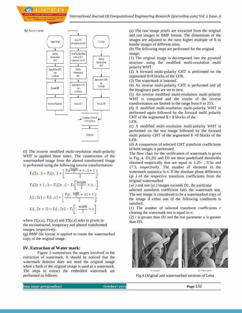
International Journal Of Computational Engineering Research (ijceronline.com) Vol. 2 Issue. 6
Issn 2250-3005(online) October| 2012 Page 132
(f) The inverse modified multi-resolution multi-polarity
WHT is applied three times. The construction of the
watermarked image from the altered transformed image
is performed using the following inverse transformation:
where I1[y,x], T1[y,x] and T3[y,x] refer to pixels in
the reconstructed, temporary and altered transformed
images, respectively.
(g) BMP file format is applied to create the watermarked
copy of the original image.
IV. Extraction of Water mark: Figure 3 summarizes the stages involved in the
extraction of watermark. It should be noticed that the
watermark detector does not need the original image
when a hash of the original image is used as a watermark.
The steps to extract the embedded watermark are
performed as follows:
(a) The raw image pixels are extracted from the original
and test images in BMP format. The dimensions of the
images are adjusted to the next higher multiple of 8 to
handle images of different sizes.
(b) The following steps are performed for the original
image:
(1) The original image is decomposed into the pyramid
structure using the modified multi-resolution multi
polarity WHT.
(2) A forward multi-polarity CHT is performed on the
segmented 8×8 blocks of the LFB.
(3) The watermark is inserted.
(4) An inverse multi-polarity CHT is performed and all
the imaginary parts are set to zero.
(5) An inverse modified multi-resolution multi-polarity
WHT is computed and the results of the inverse
transformation are limited in the range from 0 to 255.
(6) A modified multi-resolution multi-polarity WHT is
performed again followed by the forward multi polarity
CHT of the segmented 8 × 8 blocks of the
LFB.
(c) A modified multi-resolution multi-polarity WHT is
performed on the test image followed by the forward
multi polarity CHT of the segmented 8 ×8 blocks of the
LFB.
(d) A comparison of selected CHT transform coefficients
of both images is performed.
The flow chart for the verification of watermark is given
in Fig. 4. D1,D2 and D3 are three predefined thresholds
obtained empirically that are equal to 1.25 , 0.5n and
17.5, respectively. The number of elements in the
watermark sequence is n. If the absolute phase difference
(qi ) of the respective transform coefficients from the
original watermarked
(wi ) and test (yi ) images exceeds D1, the particular
selected transform coefficient fails the watermark test.
The test image is considered to be a watermarked copy of
the image if either one of the following conditions is
satisfied:
(1) The number of selected transform coefficients r
clearing the watermark test is equal to n.
(2) r is greater than D2 and the test parameter u is greater
than D3.
Fig.4.Original and watermarked versions of Lena

International Journal Of Computational Engineering Research (ijceronline.com) Vol. 2 Issue. 6
Issn 2250-3005(online) October| 2012 Page 133
The above-mentioned test parameters are defined as
follows:
Fig. 5 Watermark detector response (uniqueness of
watermark)
Fig. 6 JPEG encoded version of Lena at 10% quality and
0% smoothing.
V. Experimental results: The proposed watermarking technique has been
implemented in the C language. In order to evaluate the
proposed technique, the original grey scale image (Lena
from [2]) of 256 × 256 pixels shown in Fig. is
watermarked using the proposed scheme. The
watermarked version is shown in Fig.. The robustness of
the watermark depends directly on the embedding
strength, which in turn influences the visual degradation
of the image. The PSNR of the watermarked image with
respect to the original image is 41.34 dB. The
watermarked image is subjected to a series of tests to
gauge the robustness of the embedded watermark such
as:
(a) Uniqueness of Watermark: Fig shows the response of
the watermark detector to 1000 randomly generated
watermarks of which only one matches the watermark
embedded in Fig. . The positive response due to the
correct watermark is very much stronger than the
response due to incorrect watermark.
(b) JPEG Compression: In this test, the watermarked
image is compressed using the standard JPEG encoding .
Figure shows a JPEG encoded version of Lena at 10%
quality factor and 0% smoothing. The embedded
watermark is still detected even though the JPEG
encoded image is clearly distorted. Table 1 lists the
results for the JPEG compression tests from 10% to
100% quality factor.
Fig. 7 Image of Lena after five successive watermarking
operations

International Journal Of Computational Engineering Research (ijceronline.com) Vol. 2 Issue. 6
Issn 2250-3005(online) October| 2012 Page 134
Fig. 8 Watermark detector response (successive
watermarking)
(c) Successive watermarking: The original image is
watermarked, the watermarked image is then
watermarked and so on. This can be considered as
another form of attack in which it is clear that significant
image degradation eventually occurs as the process is
repeated. After five successive watermarking operations,
the five watermarks are still detected in the resulting
image (PSNR = 31.18 dB) shown in Fig.7. In the
response of the watermark detector given in Fig.8, the
five spikes clearly indicate the presence of the
watermarks and demonstrate that successive
watermarking does not remove the embedded
watermarks.
VI. Conclusion: A new hybrid technique for watermarking grey
scale images based on the multi-resolution modified
multi-polarity WHT and CHT is proposed and developed.
The quality of the watermarked image is very good. The
proposed technique also exhibits robustness to JPEG
compression up to 10% quality factor, successive
watermarking, sharpening, dithering distortion (25%),
cropping and scaling up to 31.64% of the original image.
References: 1. Agaian, S.S.: Hadamard Matrices and Their
Applications. Lecture Notes in Mathematics, vol.
1168. Springer, Berlin (1980)
2. CityU-IPL Image Database at
http://www.image.cityu.hk/ imagedb/
3. Cox, I.J., Killian, J., Leighton, F.T., Shamoon, T.:
Secure spread spectrum watermarking for
multimedia. IEEE Trans. Image Process. 6(12),
1673–1687 (1997)
4. Falkowski, B.J.: Properties and ways of
calculation of multi polarity generalized Walsh
transforms. IEEE Trans. Circuits Syst. II: Analog
Digit. Signal Process. 41(6), 380–391 (1994)
5. Falkowski, B.J.: Family of generalized multi-
polarity complex Hadamard transforms. IEE
Proc. Vis. Image Signal Process. 145(6), 371–378
(1998)
6. Falkowski, B.J., Rahardja, S.: Complex
Hadamard transforms: properties, relations and
architecture. IEICE Trans. Fundam. Electron.
Commun. Comput. Sci. E87-A(8), 2077–2083
(2004)
7. Jahne, B.: Digital Image Processing, 5th edn.
Springer, Berlin (2002)
8. Ó Ruanaidh, J.J.K., Dowling, W.J., Boland, F.M.:
Watermarking digital images for copyright
protection. IEE Proc. Vis. Image Signal Process.
143(4), 250–256 (1996)
9. Ó Ruanaidh, J.J.K., Dowling, W.J., Boland, F.M.:
Phase watermarking of digital images. In: Proc.
IEEE Int. Conf. on Image Processing, pp. 239–
242 (1996)
10. Plataniotis, K.N., Venetsanopoulos, A.N.: Color
Image Processing and Applications. Springer,
Berlin (2000)
11. Proakis, J.G.: Digital Communications, 4th edn.
McGraw-Hill, New York (2001)
12. Rahardja, S., Falkowski, B.J.: Comparative study
of discrete orthogonal transforms in adaptive
signal processing. IEICE Trans. Fundam.
Electron. Commun. Comput. Sci. E82-A(8),
1386–1390 (1999)
13. Rahardja, S., Falkowski, B.J.: Family of unified
complex
Hadamard transforms. IEEE Trans. Circuits Syst.
II: Analog Digit. Signal Process. 46(8), 1094–
1100 (1999)
14. Rahardja, S., Falkowski, B.J.: Complex
composite spectra of unified complex Hadamard
transform for logic functions. IEEE Trans.
Circuits Syst. II: Analog Digit. Signal Process.
47(11), 1291–1297 (2000)
15. Rahardja, S., Ser, W., Lin, Z.: UCHT-based
complex sequences for asynchronous CDMA
system. IEEE Trans. Commun. 51(4), 618–626
(2003)
16. Robin, M., Poulin, M.: Digital Television
Fundamentals: Design and Installation of Video
and Audio Systems. McGraw-Hill, New York
(1998)
17. Rojaini, K.B.: Programming in C with Numerical
Methods for Engineers. Prentice Hall, Englewood
Cliffs (1996) 1

International Journal Of Computational Engineering Research (ijceronline.com) Vol. 2 Issue. 6
Issn 2250-3005(online) October| 2012 Page 135
18. Swanson, M.D., Kobayashi, M., Tewfik, A.H.:
Multimedia dataembedding and watermarking
techniques. Proc. IEEE 86(6),1064–1087 (1998)
19. Tian, J.: Wavelet-based reversible watermarking
for authentication.In: Proc. SPIE Security and
Watermarking of Multimedia Contents IV, San
Jose, USA, pp. 679–690 (2002)
20. Wallace, G.K.: The JPEG still picture
compression standard. Commun.ACM 34(4), 30–
44 (1991)
21. Xie, S., Rahardja, S.: Performance evaluation for
quaternary DSSSMA communications with
complex signature sequences over Rayleigh-
fading channels. IEEE Trans. Wirel. Commun.
4(1), 266–277 (2005)
22. Yaroslavsky, L.P.: Digital Picture Processing.
Springer, Berlin (1985)
AUTHORS:
Mr.SK. Khamuruddeen working as an Assistant
Professor in Hyderabad Institute of Technology &
Management, His area of interest is VLSI & System
Design. you can reach him.
Mrs. S. V. Devika Working as an Associate Professor in
Hyderabad Institute of Technology & Management, her
area of interest is communications, VLSI & Antenna
theory.
Neerugatti Viswanath working as Assistant Professor in
ST. Peters college of Engineering, Hyderabad and his
area of interest is signal processing and communication
engineering.
P.Prem Kishan working as an Assistant Professor in
MLRIT, His area of interest is VLSI & Signal
processing.
J.Chandra Shekar working as Assistant Professor in
ST. Peters college of Engineering, Hyderabad and his
area of interest Fiber Optic Instrumentation and
Communication, Wireless communication
G.Shravan Kumar working as an Assistant Professor in
MLRIT, His area of interest is VLSI & System Design.
Mrs. G.Swetha as an Associate Professor in ACTS, her
area of interest is communications, VLSI & Antenna
theory.

International Journal Of Computational Engineering Research (ijceronline.com) Vol. 2 Issue. 6
Issn 2250-3005(online) October| 2012 Page 136
Content Based Image Retrieval Using Multiwavelet 1N.Santhosh,
2Mrs.T.Madhavi Kumari
1 PG Scholar, Dept. Of Electronics & Communication,JNTU Kukatpally, Hyderabad.
2Associate Professor, and Co-Ordinator Of Academics, Dept. Of Electronics & Communication,JNTU Kukatpally,
Hyderabad.
Abstract— This paper presents Content Based Image Retrieval using multiwavelet. The database image features are
extracted by multiwavelet based features at different levels of decompositions. In this paper, we have tested 500 images with
11 different categories. The experimental results show the better results in terms of retrieve accuracy and computation
complexity. Euclidean Distance and Canberra Distance are used as similarity measure in the proposed CBIR system.
Index Terms— Accuracy, Energy, Euclidean distance and Canberra distance, Image retrieval, multiwavelet.
1. Introduction Content-Based Image Retrieval (CBIR) is the
process of retrieving images from a database on the basis
of features that are extracted automatically from the
images themselves [1]. A CBIR method typically converts
an image into a feature vector representation and matches
with the images in the database to find out the most
similar images. In the last few years, several research
groups have been investigating content based image
retrieval.
A popular approach is querying by example and
computing relevance based on visual similarity using
low-level image features like color histograms, textures
and shapes. Text-based image retrieval can be traced back
to the 1970‟s; images were represented by textual
descriptions and subsequently retrieved using a text-based
database management system [2].
Content-based image retrieval utilizes
representations of features that are automatically extracted
from the images themselves. Most of the current CBIR
systems allow for querying-by-example, a technique
wherein an image (or part of an image) is selected by the
user as the query. The system extracts the features of the
query image, searches through the database for images
with similar features, and displays relevant images to the
user in order of similarity to the query [3].
Image Retrieval aims to provide an effective and
efficient tool for managing large image databases.
With the ever growing volume of digital image
generated, stored, accessed and analyzed.
The paper is organized as follows. Algorithm of
proposed method is presented in Section 2. Section 3,
describes the multiwavelet. The texture image retrieval is
Presented in Section 4. Feature Similarity is made in
Section 5. Results are shown in section 6. Section 7
describes the conclusion.
2. Algorithm of Multiwavelet The algorithm of proposed method as shown
below
Select query image
For i=1: numberofdatabaseimages
x=imread(x)
S=size(x)
x=histeq(x) %apply histogram
[a1, b1, c1, d1]=multiwavelet(x);
E1=1/m*n*∑∑ a1
E2=1/m*n*∑∑ b1
E3=1/m*n*∑∑ c1
E4=1/m*n*∑∑ d1
D=Euclidian distance
T=sort (d)
End
The Euclidian distance and multi wavelet are explained in
next section.
3. Multi Wavelet Transform Multiwavelets were defined using several
wavelets with several scaling functions [7]. Multiwavelets
have several advantages in comparison with scalar
wavelet [8]. A scalar wavelet cannot possess all these
properties at the same time. On the other hand, a
multiwavelet system can simultaneously provide
perfect representation while preserving length
(Orthogonality), good performance at the boundaries
(via linear-phase symmetry), and a high order of
approximation (vanishing moments) [9]. Thus
multiwavelets offer the possibility of superior
performance and high degree of freedom for image
processing applications, compared with scalar wavelets.

International Journal Of Computational Engineering Research (ijceronline.com) Vol. 2 Issue. 6
Issn 2250-3005(online) October| 2012 Page 137
During a single level of decomposition using a scalar
wavelet transform, the 2- D image data is replaced by
four blocks corresponding to the sub bands
representing either low pass or high pass in both
dimensions. These sub bands are illustrated in Fig. 3.
The multi-wavelets used here have two channels, so
there will be two sets of scaling coefficients and two
sets of wavelet coefficients. Since multiple iteration
over the low pass data is desired, the scaling
coefficients for the two channels are stored together.
Likewise, the wavelet coefficients for the two
channels are also stored together
.
L1L1 L1L2 L1H1 L1H2
L2L1 L2L2 L2H1 L2H2
H1L1 H1L2 H1H1 H1H2
H2L1 H2L2 H2L1 H2L2
Fig.1. Image decomposition after a single level
scaling for multiwavelets
4. Texture Image Retrival Procedure The multi wavelet is calculated of each image
from the database. The multi wavelet decomposed in to 16
sub bands then calculate the energies of 16 sub bands and
those energy values are arranged in a row vector.
For example
Energy= [e1 e2 e3 -------e16];
Where
e1, e2, e3 are the energy values of each sub band.
Calculate the energy of all decomposed images at the
same scale, using:
------ (1)
Where M and N are the dimensions of the image, and X is
the intensity of the pixel located at row „i‟ and column „j‟
in the image map. These energy level values are stored to
be used in the Euclidean distance algorithm.
5. Feature Similarities
In this section, we are using Canberra distance and
Euclidean distance to measure the similarity between
Database images and query image.
Canberra distance between two vectors P and Q is given
by
------- (2)
Here,
Pi is the energy vector of Query mage
Qi is the energy vector of database images.
The Euclidean distance is given by
D= (sum ((ref-dbimg). ^2). ^0.5)
Here
ref is the query image vector
dbimg is the database image vector.
In equation 2 the numerator signifies the difference and
denominator normalizes the difference. Thus distance
values will never exceed one, being equal to one
whenever either of the attributes is zero.
The performance is measured in terms of the average
retrieval rate, which is defined as the average percentage
number of patterns belonging to the same image as the
query pattern in the top 20 matches.
6. Results The proposed system is developed on matlab
tool for the evaluation of performance metrics. The
obtained simulation results were processed on coil
database images. The simulative result obtained are
illustrated below
Fig.2.Query image of mango coil
Fig.3.similarity image retrivals using multiwavelet

International Journal Of Computational Engineering Research (ijceronline.com) Vol. 2 Issue. 6
Issn 2250-3005(online) October| 2012 Page 138
In fig 3. It retrive 8 simirality images out of 9 image.
So the accuracy is 88%.
We can also retrive images which contain human faces
with 100% accuracy by using multiwaavelets.
Fig.4. Query image
Fig.5.similarity image retrivals using multiwavelet
In fig 5. It retrive 9 simirality images out of 9 image. So
the accuracy is 100%
It takes 1 minute 3 sec time of 500 images. In Gabor
wavelet takes around 5-6 minutes time. So the
computation time is less compare to Gabor wavelet.
7. Conclusion This paper presents image retrieval based on
multiwavelet has been proposed. It is better accuracy and
computation complexity is low. The computational steps
are effectively reduced with the use of multiwavelet. As a
result, there is a substation increase in the retrieval
speed. The whole indexing time for the 500 image
database takes 1 minute 3 seconds.
References [1] J Eakins, M E Graham, Content-based Image
Retrieval, A report to the JISC Technology
Applications Programme, 1999.
[2] Thomas S. Huang, Yong Rui, and Shinh-Fu Chang,
Image retrieval: Past, Present and Future,
International Symposium on Multimedia
Information Processing, 1997.
[3] M. Myron Flickner, H. Sawhney, W. Niblack, J.
Ashley, Q. Huang, B. Dom, M. Gorkani, J.
Hafner, D. Lee, D.Petkovic, D.Steele and
P.Yanker, “Query by image content: The QBIC
system”, In IEEE Computer, pp. 23-31, Sept.1995
[4] Patrick M. Kelly, Michael Cannon and Donald R.
Hush, Query by Image Example: The CANDID
approach. In Storage and Retrieval for Image and
Video Databases III, volume 2420, pp 238-248,
SPIE, 1995
[5] Chad Carson, Serge Belongie, Hayit Greenspan,
Jitendra Malik, Blobworld: Image segmentation
using Expectation-Maximization and its
application to image querying, Third International
Conference on Visual Information Systems, 1999
[6] M. Das, E. M. Riseman, and B. A. Draper. Focus:
Searching for multi-colored objects in a diverse
image database, In IEEE Conference on Computer
Vision and Pattern Recognition, pp 756-761, Jun
1997
[7] S. Satini, R. Jain. Similarity Measures. IEEE
Transactions on pattern analysis and machine
Intelligence, Vol.21, No.9, pp 871-883,
September 1999.
[8] Hiremath.P.S, Shivashankar . S. Wavelet based
features for texture classification, GVIP Journal,
Vol.6, Issue 3, pp 55-58, December 2006.
[9] B. S. Manjunath and W.Y. Ma. Texture Feature for
Browsing and Retrieval of Image Data. IEEE
Transactions on Pattern Analysis and Machine
Intelligence, Vol. 8, No. 8, 1996.
Author’s profile:
.
N.Santhosh, received Bachelor‟s Degree
in Electronics and Communications from
JNTU, Hyd. Then he worked as a
Asst.Professor in Dept. of ECE in Aurora‟s
Scientific and Technological Institute,
Ghatkesar, R.R.Dist. Presently he is
Pursuing his M.Tech in Digital Systems
and Computer Electronics in JNTU
Kukatpally, Hyderabad.
Mrs.Thoomati Madhavi Kumari obtained
B.Tech. in ECE and M.Tech. in Computer
Science from JNT University. Presently Mrs.
Madhavi is pursuing Ph.D. in Data security
for natural languages using FPGA. Mrs.
Madhavi joined the faculty of ECE
Department of JNU College of Engineering,
Kukatpally, Hyderabad as Assistant
Professor and served the department for 13
years. Later she was appointed as Assistant
Director, UGC-ASC, JNT University, and
Hyderabad. She was associated with the
implementation of AICTE sponsored project
on computer networks.

International Journal Of Computational Engineering Research (ijceronline.com) Vol. 2 Issue. 6
Issn 2250-3005(online) October| 2012 Page 139
Caching Strategies Based on Information Density Estimation in Wireless
Ad Hoc Networks
1D.Nagaraju,
2L.Srinivasa rao,
3K.Nageswara Rao
123Sathupally MIST Khammam, Andhra Pradesh, India
Abstract: We address cooperative caching in wireless networks, where the nodes may be mobile and exchange information in a peer-to-
peer fashion. We consider both cases of nodes with largeand small-sized caches. For large-sized caches, we devise a strategy
where nodes, independent of each other, decide whether to cache some content and for how long. In the case of small-sized
caches, we aim to design a content replacement strategy that allows nodes to successfully store newly received information
while maintaining the good performance of the content distribution system. Under both conditions, each node takes decisions
according to its perception of what nearby users may store in their caches and with the aim of differentiating its own cache
content from the other nodes’. The result is the creation of content diversity within the nodes neighborhood so that a
requesting user likely finds the desired information nearby. We simulate our caching algorithms in different ad hoc network
scenarios and compare them with other caching schemes, showing that our solution succeeds in creating the desired content
diversity, thus leading to a resource-efficient information access.
Index Terms— Data caching, mobile ad hoc networks.
I. Introduction PROVIDING information to users on the move is one of
the most promising directions of the infotainment
business, which rapidly becomes a market reality, because
infotainment modules are deployed on cars and handheld
devices. The ubiquity and ease of access of third- and
fourth-generation (3G or 4G) networks will encourage
users to constantly look for content that matches their
interests. However, by exclusively relying on
downloading from the infrastructure, novel applications
such as mobile multimedia are likely to overload the
wireless network (as recently happened to AT&T
following the introduction of the iPhone [1]). It is thus
conceivable that a peer-to-peer system could come in
handy, if used in conjunction with cellular networks, to
promote content sharing using ad hoc networking among
mobile users [2]. For highly popular content, peer-to-peer
distribution can, indeed, remove
• Large-sized caches.
In this case, nodes can potentially store a large portion
(i.e., up to 50%) of the available information items.
Reduced memory usage is a desirable (if not required)
condition, because the same memory may be shared by
different services and applications that run at nodes. In
such a scenario, a caching decision consists of computing
for how long a given content should be stored by a node
that has previously requested it, with the goal of
minimizing the memory usage without affecting the
overall information retrieval performance;
• Small-sized caches.
In this case, nodes have a dedicated but limited amount of
memory where to store a small percentage (i.e., up to
10%) of the data that they retrieve. The caching decision
translates into a cache replacement strategy that selects
The information items to be dropped among the
information items just received and the information items
that already fill up the dedicated memory. We evaluate
the performance of Hamlet in different mobile network
scenarios, where nodes communicate through ad hoc
connectivity. The results show that our solution ensures a
high query resolution ratio while maintaining the traffic
load very low, even for scarcely popular content, and
consistently along different network connectivity and
mobility scenarios.
A. Cooperative Caching
Distributed caching strategies for ad hoc networks are
presented according to which nodes may cache highly
popular content that passes by or record the data path and
use it to redirect future requests. Among the schemes
presented in [9], the approach called Hybrid Cache best
matches the operation and system assumptions that we
consider; we thus employ it as a benchmark for Hamlet in
our comparative evaluation. In [10], a cooperative
caching technique is presented and shown to provide
better performance than Hybrid Cache. However, the
solution that was proposed is based on the formation of an
overlay network composed of ―mediator‖ nodes, and it is
only fitted to static connected networks with stable links
among nodes. These assumptions, along with the
significant communication overhead needed to elect
―mediator‖ nodes, make this scheme unsuitable for the
mobile environments that we address. The work in [11]
proposes a complete framework for information retrieval
and caching in mobile ad hoc networks, and it is built on
an underlying routing protocol and requires the manual
setting of a networkwide ―cooperation zone‖ parameter.
Note that assuming the presence of a routing protocol can
prevent the adoption of the scheme in [11] in highly
mobile networks, where maintaining network connectivity

International Journal Of Computational Engineering Research (ijceronline.com) Vol. 2 Issue. 6
Issn 2250-3005(online) October| 2012 Page 140
is either impossible or more communication expensive
than the querying/ caching process. Furthermore, the need
of a manual calibration of the ―cooperation zone‖ makes
the scheme hard to configure, because different
environments are considered. Conversely, Hamlet is self
contained and is designed to self adapt to network
environments with different mobility and connectivity
features. One vehicular ad hoc network scenario is
addressed in [12], where the authors propose both an
information retrieval technique that aims at finding the
most popular and relevant data matching a user query and
a popularity-aware data replacement scheme. The latter
approach ensures that the density of different content is
proportional to the content’s popularity at the system
steady state, thus obeying the square-root rule proposed in
[13] for wired networks. We point out that the square-root
rule does not consider where copies of the data are located
but only how many copies are created. It is thus
insufficient in network environments whose dynamism
makes the positioning of content of fundamental
importance and renders steady-state conditions (as
assumed in [13]) hard to be achieved.
B. Content Diversity
Similar to Hamlet, in [6], mobile nodes cache data items
other than their neighbors to improve data accessibility. In
particular, the solution in [6] aims at caching copies of the
same content farther than a given number of hops. Such a
scheme, however, requires the maintenance of a
consistent state among nodes and is unsuitable for mobile
network topologies. The concept of caching different
content within a neighborhood is also exploited in [7],
where nodes with similar interests and mobility patterns
are grouped together to improve the cache hit rate, and in
[8], where neighboring mobile nodes implement a
cooperative cache replacement strategy. In both works,
the caching management is based on instantaneous
feedback from the neighboring nodes, which requires
additional messages. The estimation of the content
presence that we propose, instead, avoids such
communication overhead.
C. Caching With Limited Storage Capability
In the presence of small-sized caches, a cache
replacement technique needs to be implemented. Aside
from the scheme in [8], centralized and distributed
solutions to the cache placement problem, which aim at
minimizing data access costs when network nodes have
limited storage capacity, are presented in [14]. Although
centralized solutions are not feasible in ad hoc
environments, the distributed scheme in [14] makes use of
cache tables, which, in mobile networks, need to be
maintained similar to routing tables. Hamlet does not rely
on cache tables, and thus, it does not incur the associate
high communication penalty. In [15], a content
replacement strategy that aims at minimizing energy
consumption is proposed. To determine which content
should be discarded, the solution exploits the knowledge
of data access probabilities and distance from the closest
provider—an information that is typically hard to obtain
and is not required by Hamlet. A content replacement
scheme that addresses storage limitations is also proposed
in [6]. It employs a variant of the last recently used (LRU)
technique, which favors the storage of the most popular
items instead of the uniform content distribution targeted
by Hamlet. In addition, it exploits the cached item IDs
provided by the middleware to decide on whether to reply
to passing-by queries at the network layer, as well as link-
layer traffic monitoring to trigger prefetching and
caching. In [17], the popularity of content is taken into
account, along with its update rate, so that items that are
more frequently updated are more likely to be discarded.
Similarly, in [18], cache replacement is driven by several
factors, including access probability, update frequency,
and retrieval delay. These solutions thus jointly address
cache replacement and consistency, whereas in this paper,
we specifically target the former issue. However, as will
be pointed out, Hamlet can easily be coupled with a
dedicated cache consistency scheme, e.g., [9] and [12].
2196 IEEE TRANSACTIONS ON VEHICULAR
TECHNOLOGY, VOL. 60, NO. 5, JUNE 2011
D. Data Replication
Although addressing a different problem, some
approaches to data replication are relevant to the data
caching solution that we propose. One technique of
eliminating information replicas among neighboring
nodes is introduced in [` 11], which, unlike Hamlet,
requires knowledge of the information access frequency
and periodic transmission of control messages to
coordinate the nodes’ caching decisions. In [5], the
authors propose a replication scheme that aims at having
every node close to a copy of the information and analyze
its convergence time. However, unlike Hamlet, the
scheme implies a significant overhead and an exceedingly
high convergence time, thus making it unsuitable for
highly variable networks. Finally, the work in [22] adopts
a cross-layer approach to data replication in mobile ad
hoc networks, where network-layer information on
the node movement path helps to trigger the replication
before network partitioning occurs.
Iii. System Outline and Assumptions Hamlet is a fully distributed caching strategy for wireless
ad hoc networks whose nodes exchange information items
in a peer-to-peer fashion. In particular, we address a
mobile ad hoc network whose nodes may be resource-
constrained devices, pedestrian users, or vehicles on city
roads. Each node runs an application to request and,
possibly, cache desired information items. Nodes in the
network retrieve information items from other users that
temporarily cache (part of) the requested items or from
one or more gateway nodes, which can store content or
quickly fetch it from the Internet. We assume a content
distribution system where the following assumptions
hold:

International Journal Of Computational Engineering Research (ijceronline.com) Vol. 2 Issue. 6
Issn 2250-3005(online) October| 2012 Page 141
1) A number I of information items is available to the
users, with each item divided into a number C of chunks;
2) user nodes can overhear queries for content and
relative responses within their radio proximity by
exploiting the broadcast nature of the wireless medium;
and
3) user nodes can estimate their distance in hops from the
query source and the responding node due to a hop-count
field in the messages.
Although Hamlet can work with any system that
satisfies the aforementioned three generic assumptions,
for concreteness, we detail the features of the specific
content retrieval system that we will consider in the
emainder of this paper. The reference system that we
assume allows user applications to request an information
item i (1 ≤ i ≤ I) that is not in their cache. Upon a request
generation, the node broadcasts a query message for the C
chunks of the information item. Queries for still missing
chunks are periodically issued until either the information
item is fully retrieved or a timeout expires. If a node
receives a fresh query that contains a request for
information i’s chunks and it caches a copy of one or
more of the requested chunks, it sends them back to the
requesting node through information messages. If the
node does not cache (all of) the requested chunks, it can
rebroadcast a query for the missing chunks, thus acting as
a forwarder. The exact algorithm that is followed by a
node upon the reception of a query message is detailed in
the flowchart in Fig. 1
(a). Fig. 1. Flowcharts of the processing of (a) query and
(b) information messages at user nodes.We denote the
address of the node that generated the query as asrc, the
query identifier as id, the address of the last node that
forwarded the query message as alast, and the set of
queried chunks as ¯c. The functional blocks that are the
focus of this paper are highlighted in
(b). Once created, an information message is sent back to
the query source. To avoid a proliferation of information
copies along the path, the only node that is entitled to
cache a new copy of the information is the node that
issued the query. Information messages are transmitted
back to the source of the request in a unicast fashion,
along the same path from which the request came. To this
end, backtracking information is carried and updated in
query messages. Nodes along the way either act as relays
for transit messages (if they belong to the backtracking
node sequence) or simply overhear their transmission
without relaying them. Fig. 1(b) depicts the flowchart of
the operations at a node that receives a message that
contains an information chunk. A node that receives the
requested information has the option to cache the
received content and thus become a provider for that
content to the other nodes. Determining a strategy of
taking such caching decisions is the main objective of this
paper, and as such, the corresponding decision blocks are
highlighted in Fig. 1(b).
We point out that Hamlet exploits the observation of
query and information messages that are sent on the
wireless channel as part of the operations of the content-
sharing application, e.g., the previously outlined
approach. As a consequence, Hamlet does not introduce
any signaling overhead. Furthermore, several
optimizations can be introduced to improve the
aforementioned basic scheme for the discovery of content.
Although our focus is not on query propagation, it is
important to take the query process into account, because
it directly determines the network load associated with the
content retrieval operation. While deriving the results, we
consider the following two approaches to query
propagation. 1) Mitigated flooding. This approach limits
the propagation range of a request by forcing a time to
live (TTL) for the query messages. In addition, it avoids
the forwarding of already-solved requests by making the
nodes wait for a query lag time before rebroadcasting a
query;
2) Eureka [13]. This approach extends mitigated flooding
by steering queries toward areas of the network where the
required information is estimated to be denser. Note that
this paper focuses on cooperative caching and we do not
tackle information consistency; thus, we do not take into
account different versions of the content in the system
model. We note, however, that the previous version of
this paper [14] jointly evaluated Hamlet with a basic
scheme for weak cache consistency based on an epidemic
diffusion of an updated cache content and we showed that
weak consistency can be reached, even with such a simple
approach, with latencies on the order of minutes for large
networks. If prompter solutions are sought, Hamlet lends
itself to be easily integrated with one
of the existing consistency solutions found in the
literature (e.g., [9], [12], [15], ). In particular, these works
propose push, pull, or hybrid approaches to achieve
different levels of cache consistency. In the case of
Hamlet, a push technique can be implemented through the
addition of invalidation messages broadcast by gateway
nodes, whereas information providers can pull an updated
content (or verify its freshness) before sending the
information to querying nodes. In either case, no major
modification of the Hamlet caching scheme is required:
the only tweaking can consist of resetting the estimation
of the infor-mation presence upon the
notification/detection of an updated version to ease the
diffusion of the new information.
IV. Hamlet Framework The Hamlet framework allows wireless users to take
caching decisions on content that they have retrieved
from the network. The process that we devise allows users
to take such decisions by leveraging a node’s local
observation, i.e., the node’s ability to overhear queries
and information messages on the wireless channel. In
particular, for each information item, a node records the
distance (in hops) of the node that issues the query, i.e.,
where a copy of the content is likely to be stored, and the
distance of the node that provides the information. Based
International Journal Of Computational Engineering Research (ijceronline.com) Vol. 2 Issue. 6
Issn 2250-3005(online) October| 2012 Page 142
on such observations, the node computes an index of the
information presence in its proximity for each of the I
items. Then, as the node retrieves content that it
requested, it uses the presence index of such an
information item to determine Fig. 2. whether a copy of
the content should be cached, for how long, and possibly
which content it should replace. By doing so, a node takes
caching decisions that favor high content diversity in its
surroundings, inherently easing the retrieval of data in the
network. Note that our technique works on a per-item
basis, and its results apply to all chunks that belong to the
same content. In the following sections, we first detail
how a node estimates the presence of information chunks
in its proximity. Next, we separately describe the role of
the information presence index in caching decisions for
nodes with large- and small-sized caches. In the former
case, the information presence index determines the cache
content drop time, whereas in the latter case, it drives the
cache content replacement.
A. Information Presence Estimation
We define the reach range of a generic node n as its
distance from the farthest node that can receive a query
generated by node n itself. As an example, in an ideal
setting in which all nodes have the same radio range, the
reach range is given by the product of the TTL and the
node radio range. Next, we denote by f the frequency at
which every node estimates the presence of each
information item within its reach range, and we define as
1/f the duration of each estimation step (also called time
step hereafter). A node n uses the information that was
captured within its reach range during time step j to
compute the following two quantities: 1) a provider
counter by using application-layer data and 2) a transit
counter by using data that were collected through channel
overhearing in a cross-layer fashion. These counters are
defined as follows.
• Provider counter dic(n, j). This quantity accounts for the
presence of new copies of information i’s chunk c,
delivered by n to querying nodes within its reach range,
during step j. Node n updates this quantity every time it
acts as a provider node (e.g., node P in the upper plot of
Fig. 2).
• Transit counter ric(n, j). This quantity accounts for the
presence of new copies of information i’s chunk c,
transferred between two nodes within n’s reach range and
FIORE et al.: CACHING STRATEGIES BASED ON
INFORMATION DENSITY ESTIMATION IN AD HOC
NETWORKS 2201 replacement schemes in [9] and [14].
It is composed of 300 wireless nodes deployed over a
square area of a side equal to 200 m. Nodes can be static,
positioned according to a uniform random distribution, or
mobile, wandering according to a random-direction
mobility model with reflections. The node speed is
uniformly distributed in the range [0.5vm, 1.5vm], where
vm is the average node speed—a varying parameter in our
simulations. The node radio range is set to 20 m,
resulting, for static nodes, in a fully connected network. In
all the scenarios, we deploy two fixed gateway nodes at
opposite ends of the topology. Each gateway permanently
stores 1/2 of the information items, whereas the other half
is provided by the other gateway. Initially, nodes have an
empty cache; they randomly request any among the I
items that are not in their cache according to a Poisson
process with parameter λi = Λqi (1 ≤ i ≤ I). Λ is the query
generation rate per node, whereas qi represents the
content popularity level (i.e., the probability that, among
all possible content, a node requests item i). The TTL
value for query messages is set to ten and five hops for
the case of large- and small-sized caches, respectively,
and the query lag time is 50 ms. Note that the impact of
all the aforementioned query propagation parameters on
the information-sharing behavior has been studied in [23];
here, we only consider what has been identified as a good
parameter setting. With regard to the Hamlet parameters,
the estimation frequency is such that 1/f = 0.2MC; indeed,
through extensive simulations, we observed that the
impact of f is negligible, as long as 1/f is not greater than
20% of the maximum caching time. As we fix τ = fMC,
this setting of f leads to a value of τ as small as 5. Then,
we have α = 0.9 andW = 0.5; indeed, we have verified that
this combination yields a smoother behavior of the
presence index pi(n, j). The values of the remaining
parameters are separately specified for large- and small-
sized caches. The information-sharing application lies on
top of a User Datagram Protocol (UDP)-like transport
protocol, whereas, at the media access control (MAC)
layer, the IEEE 802.11 standard in the promiscuous mode
is employed. No routing algorithm is implemented:
queries use a MAC-layer broadcast transmission, and
information messages find their way back to the
requesting node following a unicast path. Information
messages exploit the request to send/clear to send
(RTS/CTS) mechanism and MAC-level retransmissions,
whereas query messages of broadcast nature do not use
RTS/CTS and are never retransmitted. The channel
operates at 11 Mb/s, and signal propagation is reproduced
by a two-ray ground model. Simulations were run for 10
000 s. In the aforementioned scenarios, our performance
evaluation hinges upon the following quite-
comprehensive set of metrics that are aimed at
highlighting the benefits of using Hamlet in a distributed
scenario:
1) the ratio between solved and generated queries, called
solved-queries ratio;
2) the communication overhead;
3) the time needed to solve a query;
4) the cache occupancy.
We have further recorded the spatiotemporal distribution
of information and the statistics of information survival,
because they help in quantifying the effectiveness of
Hamlet in preserving access to volatile information. As
aforementioned, we did not explore the problem of cache
consistency, because such an
issue is orthogonal to this paper.

International Journal Of Computational Engineering Research (ijceronline.com) Vol. 2 Issue. 6
Issn 2250-3005(online) October| 2012 Page 143
Vi. Evaluation With Large-Sized Caches Here, we evaluate the performance of Hamlet in a
network of nodes with large storage capabilities, i.e., with
caches that can store up to 50% of all information items.
Because such characteristics are most likely found in
vehicular communication devices, tablets, or
smartphones, the network environments under study are
the City and Mall scenarios. As discussed in Section IV,
in this case, the Hamlet framework is employed to
compute the caching time for information chunks
retrieved by nodes, with the goal of improving the content
distribution in the network while keeping the resource
consumption low.
We first compare Hamlet’s performance to the
results obtained with a deterministic caching strategy,
called DetCache, which simply drops cached chunks after
a fixed amount of time. Then, we demonstrate the
effectiveness of Hamlet in the specific task of information
survival. In all tests, we assume I = 10 items, each
comprising C = 30 chunks. All items have identical
popularity, i.e., all items are requested with the same
rate λ = Λ/I by all network nodes. The choice of equal
request rates derives from the observation that, in the
presence of nodes with a large-sized memory, caching an
information item does not imply discarding another
information item; thus, the caching dynamics of the
different items are independent of each other and only
depend on the absolute value of the query rate. It follows
that considering a larger set of items would not change
the results but only lead to more time-consuming
simulations. Each query includes 20 B plus 1 B for each
chunk request, whereas information messages include a
20-B header and carry a 1024-B information chunk. The
maximum caching time MC is set to 100 s, unless
otherwise specified. Queries for chunks that are still
missing are periodically issued every 5 s until either the
information is fully retrieved or a timeout that is set to 25
expires.
A. Benchmarking Hamlet
We set the deterministic caching time in DetCache to 40
s, and we couple DetCache and Hamlet with both the
mitigated flooding and Eureka techniques for query
propagation. We are interested in the following two
fundamental metrics: 1) the ratio of queries that were
successfully solved by the system and 2) the amount of
query traffic that was generated. The latter metric, in
particular, provides an indication of the system
effectiveness in preserving locally rich information
content: if queries hit upon the sought information in one
or two hops, then the query traffic is obviously low.
However, whether such a wealth of information is the
result of a resource-inefficient cache-all-you-see strategy
or a sensible cooperative strategy, e.g., the approach
fostered by Hamlet, remains to be seen. Thus, additional
metrics that are related to cache occupancy
TABLE I AVERAGE OCCUPANCY OF THE NODE
CACHES, EXPRESSED AS A PERCENTAGE OF THE
CHUNKS TOTAL NUMBER FOR λ = 0.003 and
information cache drop time must be coupled with the
aforementioned metrics. Fig. 5 shows the solved-queries
ratio (top plot) and the amount of query traffic (bottom
plot) as λ varies in the City scenario. When DetCache is
used, the higher the query rate, the larger the number of
nodes that cache an information item. This case implies
that content can be retrieved with higher probability and
also that it is likely to be found in the proximity of the
requesting node, thus reducing the query traffic per issued
request. Note that, due to its efficient query propagation
mechanism, Eureka reduces the propagation of useless
queries (and,hence, collisions), yielding a higher solved-
queries ratio than mitigated flooding. However, it is
evident that deterministic caching does not pay off as
much as cooperative caching does in Hamlet. Table I
shows that the average occupancy of node caches in
Hamlet is comparable to the values observed with
DetCache. Thus, it is the quality, not the quantity, of the
information cached by Hamlet that allows it to top a
sophisticated propagation scheme such as Eureka as far as
the solved-queries ratio is concerned. The positive effect
of the caching decisions can also be observed in Fig. 5 in
terms of the reduced overhead and latency
TABLE II
AVERAGE QUERY SOLVING TIME (IN SECONDS),
WITH λ = 0.003 in solving queries. Indeed, Hamlet
reduces the overhead by shortening the distance between
requesting nodes and desired information content.
Similarly, Table II shows how sensible caching choices
can significantly reduce the time required to solve
queries, again due to the homogeneous availability of
information that they generate in the network. Further
proof of such virtuous behavior by Hamlet is provided in
Fig. 6, where mitigated flooding is used for query
propagation. The figure depicts the time evolution of
content presence over the road topology for one
information item; in particular, the z-axis of each plot
shows the fraction of different chunks that comprise an
information item that are present in a squared area of 600
m2. On the one hand, it can be observed that mitigated
flooding with DetCache creates a sharp separation
between the area where the content source resides,
characterized by high item availability, and the region
where, due to vehicular traffic dynamics, information-
carrying nodes rarely venture. On the other hand, Hamlet
favors the diffusion of content over the entire scenario so
that nodes in areas away from the information source can
also be served. Fig. 7 refers to the Mall scenario. The poor
performance of Eureka in this case is due to the lack of
information items over large areas of the Mall scenario,
resulting in queries not being forwarded and, thus,
remaining unsolved [13]. Interestingly, Hamlet greatly
reduces the query traffic for any λ, although providing a
much higher solved-queries ratio. With regard to the
caching occupancy, because Hamlet leads to results that
are comparable with the results obtained with DetCache
(see Table I, Mall scenario), it can be asserted that the
performance gain achieved through Hamlet is due to the
International Journal Of Computational Engineering Research (ijceronline.com) Vol. 2 Issue. 6
Issn 2250-3005(online) October| 2012 Page 144
more uniform content distribution across node caches.
Finally, Table II confirms that such an improved
availability of information shortens the waiting time to
receive requested items. When comparing results obtained
from the Mall and City scenarios, we note that the solved-
queries ratio is consistently lower. We recall that
vehicular mobility in the City environment is
characterized by scattered connectivity but high node
speed, whereas the Mall environment provides a better
network connectivity level but reduced node mobility.
The low node mobility in the Mall keeps items away from
the sources of unpopular items for long periods of time.
Thus, the probability of solving requests for such rare
content is low, unless an efficient caching scheme allows
nodes to preserve at least a few copies of every item in
every neighborhood, as Hamlet does. It is also worth
pointing out that, with respect to the City environment,
the Mall includes a smaller number of nodes; thus, fewer
queries are issued, and a much smaller amount of query
traffic is generated. Finally, we may wonder how well
Hamlet performs with respect to DetCache when the
cache time employed by the latter approach is set to a
value other than 40 s. Through extensive 2206 IEEE
TRANSACTIONS ON VEHICULAR TECHNOLOGY,
VOL. 60, NO. 5, JUNE 2011 Fig. 13. Memory-
constrained mobile nodes: Query-solving ratio for each
information item when using HybridCache and Hamlet,
with I = 300. The plots refer to vm that is equal to 1 m/s
(left) and 15 m/s (right). Furthermore, it is not only the
sheer quantity of data that makes a difference but its
spatial distribution also plays a major role. If several
nodes cache a rare item but they are all very close to each
other, queries that were generated in other areas of the
network take more hops to be satisfied. This case happens
with HybridCache, as proven by the spatial distribution
of the 100th, 200th, and 300th items, as shown in Fig.
12(a). Conversely, the spatial distribution achieved by
Hamlet, as shown in Fig. 12(b), is more uniform, leading
to a faster more likely resolution of queries. We now
compare the performance of HybridCache and Hamlet in
the scenario with memory-constrained mobile nodes. We
test the two schemes when I = 300 and for an average
node speed vm equal to 1 and 15 m/s. The solved-queries
ratio recorded with HybridCache and Hamlet on a per-
item basis are shown in Fig. 13. Comparing the left and
right plots, we note that the node mobility, even at high
speed, does not seem to significantly affect the results due
to the high network connectivity level. The spatial
redistribution of content induced by node movements
negatively affects the accuracy of Hamlet’s estimation
process, which explains the slight reduction in the solved
query ratio at 15 m/s. That same movement favors
HybridCache, at least at low speed, because it allows
unpopular information to reach areas that are far from the
gateway. However, the difference between the two
schemes is evident, with Hamlet solving an average of
20% requests more than HybridCache, when nodes move
at 15 m/s. Note that, for the query resolution delay and the
average cache utilization at the network nodes, we
obtained qualitatively
similar results as in the static case, with Hamlet achieving
more homogeneous solving times and fairer distribution
of content in the network than HybridCache. B. Impact of
the Zipf Distribution Skewness Finally, we study the
impact of the Zipf distribution exponent on the
performance of the cache replacement strategies. We
recall that an exponent that is equal to zero implies perfect
homogeneity, i.e., Zipf distribution that degenerates into a
uniform distribution, whereas the difference in popularity
among content becomes much more unbalanced as the
exponent grows. We focus on a network where ten items
are available and each node can cache at most one
complete item. The choice of this setting is mandated by
the fact that, in the presence of Fig. 14. Memory-
constrained static (top) and mobile (bottom) nodes:
Solvedqueries ratio and query traffic as the Zipf
distribution exponent varies when using HybridCache and
Hamlet, with I = 10. hundreds of different items,
unbalanced popularity distributions (i.e., exponents higher
than 0.5) lead to very low λi for the 100 or so least
popular items, thus making requests for such content
extremely rare. Fig. 14 depicts the evolution of the
solved-queries ratio and the query traffic as the Zipf
exponent ranges vary. By comparing the two plots, we
note that the presence of mobility (vm = 1 m/s) leads to a
higher number of unsolved requests and in a larger
amount of traffic generated within the network under
HybridCache, because queries propagate far from the
source without finding the desired item. However, what is
most interesting is how the network load tends to decrease
as the Zipf exponent grows, both in the absence and
presence of node movements. On the one hand, higher
values of the exponent lead to more unbalanced query
rates, with very few items that are extremely popular and
a long tail of seldom-accessed data.
Being requested so often, popular items become
commonly found in nodes caches, and the relative queries
are solved faster, generating small traffic. On the other,
when the Zipf exponent is small, the distribution of
queries is more balanced, with information more evenly
distributed in the network. This case implies that items
can usually be found but are hardly cached very close to
the requesting node. Thus, the different items are all
requested at a fairly high rate but are not immediately
found, generating larger query traffic.
VIII. Conclusion We have introduced Hamlet, which is a caching strategy
for ad hoc networks whose nodes exchange information
items in a peer-to-peer fashion. Hamlet is a fully
distributed scheme FIORE et al.: CACHING
STRATEGIES BASED ON INFORMATION DENSITY
ESTIMATION IN AD HOC NETWORKS 2207 where
each node, upon receiving a requested information,
determines the cache drop time of the information or
which content to replace to make room for the newly
arrived information. These decisions are made depending
on the perceived ―presence‖ of the content in the node’s
proximity, whose estimation does not cause any
additional overhead to the information sharing system.

International Journal Of Computational Engineering Research (ijceronline.com) Vol. 2 Issue. 6
Issn 2250-3005(online) October| 2012 Page 145
We showed that, due to Hamlet’s caching of information
that is not held by nearby nodes, the solving probability of
information queries is increased, the overhead traffic is
reduced with respect to benchmark caching strategies, and
this result is consistent in vehicular, pedestrian, and
memoryconstrained scenarios. Conceivably, this paper
can be extended in the future by addressing content
replication and consistency. The procedure for
information presence estimation that was developed in
Hamlet can be used to select which content should be
replicated and at which node (even if such a node did not
request the content in the first place). In addition, Hamlet
can be coupled with solutions that can maintain
consistency among copies of the same information item
cached at different network nodes, as well as with the
versions stored at gateway nodes.
References [1] J. Wortham (2009, Sep.). Customers Angered as
iPhones Overload AT&T. The New York Times.
[Online]. Available: http://www.nytimes.
com/2009/09/03/technology/companies/03att.html
[2] A. Lindgren and P. Hui, ―The quest for a killer app
for opportunistic and delay-tolerant networks,‖ in
Proc. ACM CHANTS, 2009, pp. 59–66.
[3] P. Padmanabhan, L. Gruenwald, A. Vallur, and M.
Atiquzzaman, ―A survey of data replication
techniques for mobile ad hoc network databases,‖
VLDB J., vol. 17, no. 5, pp. 1143–1164, Aug. 2008.
[4] A. Derhab and N. Badache, ―Data replication
protocols for mobile ad hoc networks: A survey and
taxonomy,‖ IEEE Commun. Surveys Tuts., vol. 11,
no. 2, pp. 33–51, Second Quarter, 2009.
[5] B.-J. Ko and D. Rubenstein, ―Distributed self-
stabilizing placement of replicated resources in
emerging networks,‖ IEEE/ACM Trans. Netw., vol.
13, no. 3, pp. 476–487, Jun. 2005.
[6] G. Cao, L. Yin, and C. R. Das, ―Cooperative cache-
based data access in ad hoc networks,‖ Computer,
vol. 37, no. 2, pp. 32–39, Feb. 2004.
[7] C.-Y. Chow, H. V. Leong, and A. T. S. Chan,
―GroCoca: Group-based peer-to-peer cooperative
caching in mobile environment,‖ IEEE J. Sel. Areas
Commun., vol. 25, no. 1, pp. 179–191, Jan. 2007.
[8] T. Hara, ―Cooperative caching by mobile clients in
push-based information systems,‖ in Proc. CIKM,
2002, pp. 186–193.
[9] L. Yin and G. Cao, ―Supporting cooperative caching
in ad hoc networks,‖ IEEE Trans. Mobile Comput.,
vol. 5, no. 1, pp. 77–89, Jan. 2006.
[10] N. Dimokas, D. Katsaros, and Y. Manolopoulos,
―Cooperative caching in wireless multimedia sensor
networks,‖ ACM Mobile Netw. Appl., vol. 13, no.
3/4, pp. 337–356, Aug. 2008.
[11] Y. Du, S. K. S. Gupta, and G. Varsamopoulos,
―Improving on-demand data access efficiency in
MANETs with cooperative caching,‖ Ad Hoc Netw.,
vol. 7, no. 3, pp. 579–598, May 2009.
[12] Y. Zhang, J. Zhao, and G. Cao, ―Roadcast: A
popularity-aware content sharing scheme in
VANETs,‖ in Proc. IEEE Int. Conf. Distrib.
Comput. Syst., Los Alamitos, CA, 2009, pp. 223–
230.
[13] E. Cohen and S. Shenker, ―Replication strategies in
unstructured peer-topeer networks,‖ in Proc. ACM
SIGCOMM, Aug. 2002, pp. 177–190.
[14] B. Tang, H. Gupta, and S. Das, ―Benefit-based data
caching in ad hoc networks,‖ IEEE Trans. Mobile
Comput., vol. 7, no. 3, pp. 289–304, Mar. 2008.
[15] W. Li, E. Chan, and D. Chen, ―Energy-efficient
cache replacement policies for cooperative caching
in mobile ad hoc network,‖ in Proc. IEEE WCNC,
Kowloon, Hong Kong, Mar. 2007, pp. 3347–3352.
D.Nagaraju pursuing M.Tech in
the department of computer Science & Engineering. His
interested areas are Network Security and dataminining.
L.Srinivasa Rao working as assistant
professor in the department of computer Science &
Engineering. His interested areas are Network Security
and dataminining
K.Nageswara Rao working as
associate professor in the department of computer Science
& Engineering. His interested areas are Network Security
and dataminining

International Journal Of Computational Engineering Research (ijceronline.com) Vol. 2 Issue. 6
Issn 2250-3005(online) October| 2012 Page 146
Design and Simulation of High Performance Low Power Control Circuits at
Gate and Layout Levels
1Venkatesh Kumar. N, 2Amritha Mulay. V, 3Mujeeb Ulla Jeelani [1] Asst.Professor, SET, Jain University, Freelance Consultant and Trainer
[2] Software Engineer, Allied Tools and Electronics, Bangalore.
[3] Software Engineer, 7 Star Technologies (A Startup), Bangalore.
Abstract: Many integrated circuits of today contain a very large
number of transistors, over 1 million in some designs. The
aim is to design a low power high performance sequencer
and program counter, analyze and simulate at gate and
layout levels. High level description language to be used to
construct layout of program counter and sequencer.
Keywords: Sequencer, Controller, Program Counter, Low
Leakage.
I. Introduction: The program counter plays a very important role in
the design of microprocessor as it supplies the main
program memory with the address of the active instruction.
The program counter is like someone pointing a finger at the
list of instructions, saying do this first, do this second, ad so
on. This is the reason program counter is sometimes called
pointer; it points to an address in memory where something
important is being stored. The sequencer is the heart of the
microprocessor, it controls the most important signals
generated in the microprocessor.
II. Circuit Implementation of Low Power High
Performance Program Counter and Sequencer
The program is stored at the beginning of the
memory with the first instruction at binary address 0000, the
second instruction at address 0001, the third at address 0010
and so on. The program counter, which is part of the control
unit, counts from 0000 to 1111.
Its job is to send to the memory the address of the
next instruction to be fetched and executed. At start, the
program counter is 0. Then, at the end of each instruction,
the program counter is incremented, in order to select the
next instruction [2].
One simple way to build this counter is to chain
edge sensitive D-registers as shown in Figure 1. This circuit
works asynchronously. The PC is reset to 0000 before each
computer run. When the computer run begins, the program
counter sends the address 0000 to the memory. The program
counter is then incremented to 0001. After the first
instruction is fetched and executed, the program counter
sends the next address 0001 to the memory. Again the
program counter is incremented. After the second
instruction is fetched and executed, the program counter
sends address 0010 to the memory. In this way, the program
counter is keeping track of next instruction to be fetched and
executed. In this work Program Counter is designed for 4 bit
and a maximum of 16 instructions can be addressed. This is
designed using 4 D-flip flops in asynchronous type. Figure 1
depicts its design.
Figure 1 Schematic view of Program counter.
The sequencer is the main part of the
microprocessor. It controls the most important signals such
as the enable and latch controls. The input to the sequencer
is the instruction code itself, as well as the phase
information. The four input AND gates serve as instruction
decoders. Depending on the type of instruction, the desired
signals are set to 1 if active, or kept at 0 to be inactive. The
schematic view of the sequencer is as shown in Figure 2.
Figure 2 Schematic view of the sequencer.

International Journal Of Computational Engineering Research (ijceronline.com) Vol. 2 Issue. 6
Issn 2250-3005(online) October| 2012 Page 147
III. Analysis of Leakage Power Consumption of
Program Counter and Sequencer
The leakage current is the current that flows
between Drain and Source when no channel is present
[2]. No current is expected to flow between drain and
source. However, a leakage current enables nA range
current to flow although the gate voltage is 0. Considering
the program counter and sequencer , the schematic
diagram of the counter is shown in Figure 1 and its layout
implementation in Figure 3 and the schematic of sequencer
in Figure 2 and its layout in Figure 4. Here, we analyze its
switching performances, in the high speed and low leakage
modes.
Figure 3 Layout of Program Counter
Figure 4 Layout of Sequencer.
In the high speed mode, the circuits works fast (900
M Hz) but consumes a significant standby current when
off (around 200 nA). This is as shown in Figure 5.
Once the option layer is set to “low leakage”, the
simulation is performed again. The low- leakage mode
features a little slower (100Mz that is approximately a
9 % speed reduction) and more than one decade less
standby current when off (5 nA). In summary, low leakage
MOS devices should be used as default devices whenever
possible. High speed MOS should be used only when
switching speed is critical. This is shown in Figure 6.
Figure 6 Low Leakage Mode.
IV. Result and Discussion of Program Counter and
Sequencer:
The simulation result of the program counter is
performed by enabling the clear input and applying the
clock signal. The number of transistors used for designing
the program counter is 54. From Figure 7 we can see that
the maximum current (Imax) consumed by this program
counter is approximately 0.5mA and the power dissipated
by this circuit is 0mW.
From Figure 7 it is evident that when the clear signal is set
high and the flip-flops are enabled, the program counter
starts counting from 0 to 15.
Figure 7 Simulation result of Program Counter.
The simulation result of the sequencer is as shown
in Figure 8. The different control signals that this sequencer
generates are displayed in Figure 8. From the figure we can
see that the control signals that are set high are RM and
LINR. Hence, when these signals are activated, the
corresponding operation performed by the microprocessor
is, the contents from the memory are latched on to the
instruction register.
The number of transistors used for designing the
controller is 294. The maximum current (Imax) consumed
by the sequencer during its operation is approximately
0.0mA and the power dissipated by this controller is 0mW.
Figure 5 High Speed Mode

International Journal Of Computational Engineering Research (ijceronline.com) Vol. 2 Issue. 6
Issn 2250-3005(online) October| 2012 Page 148
Figure 8 Simulation result of Sequencer.
The main objective of the low leakage MOS is to
reduce the Ioff current significantly, that is the small current
that flows between drain and source with a zero gate
voltage. The price to pay is a reduced Ion current. The
designer has the possibility to use high speed MOS
devices, which have high Ioff leakages but large Ion drive
currents. The size correspond to the 0.12µm technology [3].
In Figure 9 and Figure 10, the characteristics of NMOS and
PMOS is plotted. Both the low leakage MOS device has an
negligible Ioff current. Thanks to a higher threshold voltage
(0.4V rather than 0.3V) and larger effective channel length
(120nm) compared to the high speed MOS. In the work,
low leakage transistors are selected to encourage low
power design. The Ion difference is around 33%. This
means that a high speed MOS device is 33% faster than
the low leakage MOS.
Figure 9 NMOS Device Characteristics
Therefore, from the above analysis and results we can draw
conclusion that a proper selection of transistors and designs
move toward lower VDD and lower VTH reducing power
dissipation. In this way it is evident from the above
discussion that optimizing VDD and VTH is essential in low
power, high speed designs.
Figure 10 PMOS Device Characteristics
V. Conclusion and Scope for Future Work
Design, analysis and simulation of a Program
Counter and Sequencer at gate and layout levels is
presented. Both these circuits are designed for high
performance and low power. The circuits are tested and
simulated at transistor; gate and layout levels. The circuit is
also tested by varying the threshold voltage. These circuits
operates at a frequency range of 100MHz to 900MHz with a
wide operating voltage of 1.2V to 5V. The technology
employed is 120nm.
Leakage current can be reduced by adaptive body
biasing and embedding dual threshold voltage in the
proposed architecture. Power can be reduced by employing
a technique of controlling threshold voltage through
substrate bias.
References [1] T. Kuroda and T. Sakurai, "Overview of Low-power
ULSI Circuit Techniques," IEICE Trans. Electron., vol.
E78-C, no. 4, pp. 334-344, April 1995.
[2] A.L Davis, “A Data Driven Machine Architecture
Suitable for VLSI Implementation” Proc. Caltech conf.
VLSI Jan.19 79, pp.479-494
[3] K. Bernstein, et al.,” High Speed CMOS Design
Styles”. Kluwer, Boston, 1998.
[4] Horst, E, “Design of VLSI Circuits”, Springer Verlag,
1987
[5] S. Narendra, D. Antoniadis, and V. De, "Impact of
Using Adaptive Body Bias to Compensate Die-to-die V,
Yariation on Within-die V, Yartation," Proc.
ISLPED'99, pp. 229232, Aug. 1999.

International Journal Of Computational Engineering Research (ijceronline.com) Vol. 2 Issue. 6
Issn 2250-3005(online) October| 2012 Page 149
Security Enhanced Dynamic Routing using Quasigroups Mr. K.J. Pavithran Kumar
1 and Mr. D. Vivekananda Reddy
2
1M.Tech Student in Computer Science and Engineering, Sri Venkateswara University, Tirupati.
2Assistant Professor in Computer Science and Engineering Department, Sri Venkateswara University, Tirupati
Abstract—Security has become one of the major issues for data communication over wired and wireless networks. The
dynamic routing algorithm is used to randomize delivery paths for data transmission which is compatible with popular
routing protocols, such as the Routing Information Protocol in wired networks and Destination-Sequenced Distance
Vector protocol in wireless networks, without introducing extra control messages. This paper proposes the dynamic
routing algorithm with cryptography-based system design for more security in data transmission.
Key words—Security, Quasigroup cryptography-based system, dynamic routing, RIP, DSDV.
1. Introduction In the past decades, various security-enhanced measures have been proposed to improve the security of data
transmission over public networks. Existing work on security-enhanced data transmission includes the designs of
cryptography algorithms and system infrastructures and security-enhanced routing methods. Their common objectives are
often to defeat various threats over the Internet, including eavesdropping, spoofing, session hijacking, etc.
Another alternative for security-enhanced data transmission is to dynamically route packets between each source
and its destination so that the chance for system break-in, due to successful interception of consecutive packets for a session,
is slim. The intention of security-enhanced routing is different from the adopting of multiple paths between a source and a
destination to increase the throughput of data transmission (see, e.g., [1] and [2]). In particular, Lou et al. [3], [4] proposed a
secure routing protocol to improve the security of end-to-end data transmission based on multiple path deliveries. The set of
multiple paths between each source and its destination is determined in an online fashion, and extra control message
exchanging is needed. Bohacek et al. [5] proposed a secure stochastic routing mechanism to improve routing security.
Similar to the work proposed by Lou et al. [3], [4], a set of paths is discovered for each source and its destination in an
online fashion based on message flooding. Thus, a mass of control messages is needed. Yang and Papavassiliou [6] explored
the trading of the security level and the traffic dispersion.
The objective of this work is to explore a security enhanced dynamic routing algorithm based on distributed routing
information widely supported in existing wired and wireless networks. We aim at the randomization of delivery paths for
data transmission to provide considerably small path similarity (i.e., the number of common links between two delivery
paths) of two consecutive transmitted packets. The proposed algorithm should be easy to implement and compatible with
popular routing protocols, such as the Routing Information Protocol (RIP) for wired networks [7] and Destination-
Sequenced Distance Vector (DSDV) protocol for wireless networks [8], over existing infrastructures. These protocols shall
not increase the number of control messages if the proposed algorithm is adopted.
2. Problem Statement The objective of this work is to explore a security-enhanced dynamic routing algorithm based on distributed routing
information widely supported in existing networks. In general, routing protocols over networks could be classified roughly
into two kinds: distance-vector algorithms and link-state algorithms [9]. Distance-vector algorithms rely on the exchanging of
distance information among neighboring nodes for the seeking of routing paths. Examples of distance-vector-based routing
algorithms include RIP and DSDV. Link-state algorithms used in the Open Shortest Path First protocol [10] are for global
routing in which the network topology is known by all nodes. Our goal is to propose a distance-vector-based algorithm for
dynamic routing to improve the security of data transmission. Before we proceed with further discussions, our problem and
system model shall be defined.
A network could be modeled as a graph G = (N, L), where N is a set of routers (also referred to as nodes) in the
network, and L is a set of links that connect adjacent routers in the network. A path p from a node s (referred to as a source
node) to another node t (referred to as a destination node) is a set oflinks (N1, N2) (N2, N3)…(Ni, Ni+1), where s =N1, Ni+1= t ,
Nj Є N, and (Nj, Nj+1) Є L for 1≤j≤ i. Let Ps;t denote the set of all potential paths between a source node s and a destination
node t. Note that the number of paths in Ps;t could be an exponential function of the number of routers in the network, and
we should not derive Ps;t in practice for routing or analysis.
Definition 1 (path similarity). Given two paths pi and pj, the path similarity Sim(pi; pj) for pi and pj is defined as the
number of common links between pi and pj:
Sim(pi; pj)=|(Nx, Ny)|(Nx,Ny) Є pi ^(Nx, Ny) Є pj|,

International Journal Of Computational Engineering Research (ijceronline.com) Vol. 2 Issue. 6
Issn 2250-3005(online) October| 2012 Page 150
Where Nx and Ny are two nodes in the network. The path similarity between two paths is computed based on the algorithm
of Levenshtein distance [5].
Definition 2 (the expected value of path similarity for anytwo consecutive delivered packets). Given a source node s and a
destination node t, the expected value of path similarity of any two consecutive delivered packets is defined as follows:
E[Sims;t]= ∑Sim(pi, pj) . Prob(pj|pi) . Prob(pi),
where Ps;t is the set of all possible transmission paths between a source node s and a destination node t. Prob(pj|pi) is the
conditional probability of using pj for delivering the current packet, given that pi is used for the previous packet. Prob(pi) is
the probability of using pi for delivering the previous packet.
The purpose of this research is to propose a dynamic routing algorithm to improve the security of data transmission.
We define the eavesdropping avoidance problem as follows:
Given a graph for a network under discussion, a source node, and a destination node, the problem is to minimize the
path similarity without introducing any extra control messages, and thus to reduce the probability of eavesdropping
consecutive packets over a specific link.
3. Security-Enhanced Dynamic Routing 3.1. Notations and Data Structures:
The objective of this section is to propose a distance-vector based algorithm for dynamic routing to improve the
security of data transmission. We propose to rely on existing distance information exchanged among neighboring nodes
(referred to as routers as well in this paper) for the seeking of routing paths. In many distance-vector-based implementations,
e.g., those based on RIP, each node Ni maintains a routing table (see Table 1a) in which each entry is associated with a tuple
(t, WNi,t;Nexthop), where t, WNi,t, and Next hop denote some unique destination node, an estimated minimal cost to send a
packet to t, and the next node along the minimal-cost path to the destination node, respectively.
With the objective of this work in the randomization of routing paths, the routing table shown in Table 1a is
extended to accommodate our security-enhanced dynamic routing algorithm. In the extended routing table (see Table 1b),
we propose to associate each entry with a tuple (t,WNi,t, CtNi
,HtNi
). , CtNi
is a set of node candidates for the nexthop (note that
the candidate selection will be elaborated in Procedure 2 of Section 3.2), where one of the nexthop candidates that have the
minimal cost is marked. HtNi
, a set of tuples, records the history for packet deliveries through the node Ni to the destination
node t. Each tuple (Nj, hNj) in HtNi
is used to represent that Ni previously used the node hNj as the nexthop to forward the
packet from the source node Nj to the destination node t. Let Nbri and wNi,Nj denote the set of neighboring nodes for a node
Ni and the cost in the delivery of a packet between Ni and a neighboring node Nj, respectively. Each node Ni also maintains
an array (referred to as a link table) in which each entry corresponds to a neighboring node Nj Є Nbri and contains the cost
wNi,Nj for a packet delivery. The proposed algorithm achieves considerably small path similarity for packet deliveries
between a source node and the corresponding destination node. However, the total space requirement would increase to store
some extra routing information. The size of a routing table depends on the topology and the node number of a network under
discussions. In the worst case, we have a fully connected network. For each entry in the routing table shown in Table 1b, the
additional spaces requirement would increase to store some extra routing information. The size of a routing table depends on
the topology and the node number of a network under discussions. In the worst case, we have a fully connected network. For
each entry in the routing table shown in Table 1b, the additional spaces required for recording the set of node candidates (as
shown in the third column of Table 1b) and for recording the routing history (as shown in the fourth column of Table 1b) are
O(|N|). Because there are |N| destination nodes at most in each routing table, the additionally required spaces for the entire
routing table for one node are O(|N|2). Since the provided distributed dynamic routing algorithm (DDRA) is a distance-
vector-based routing protocol for intradomain systems, the number of nodes is limited, and the network topology is hardly
fully connected. Hence, the increase of the total space requirement is considerably small.
Table I: An Example Of The Routing Table For The Node Ni

International Journal Of Computational Engineering Research (ijceronline.com) Vol. 2 Issue. 6
Issn 2250-3005(online) October| 2012 Page 151
(a) The routing table for the original distance-vector-based routing algorithm.
(b) The routing table for the proposed security-enhanced routing algorithm.
3.2. A Secured Distributed Dynamic Routing Algorithm:
The DDRA proposed in this paper consists of two parts:
Applying the cryptography-based system
A randomization process for packet deliveries and
Maintenance of the extended routing table.
3.2.1. Cryptography based system
The cryptography is used to increase the security in dynamic routing algorithm. The data will be encrypted by using
the Quasigroup cryptography algorithm. Then the encrypted data is divided into packets. The encrypted packets will send to
the destination using distributed dynamic routing algorithm. The cryptography process is as follows:
Fig. 1. Cryptography-based System
The cryptography based system encrypts the data and the encrypted data will be sending to randomization process.
The randomized process will send the encrypted data to the destination through several paths. The encrypted data will be
divided into packets and each packet is send to the destination through different paths. All the packets travelled through
different paths will reach the destination and that encrypted data will undergo decryption process. The decryption process
will decrypt the data and the destination will get the secure data.
3.2.2. Randomization Process
Consider the delivery of a packet with the destination t at a node Ni. In order to minimize the probability that
packets are eavesdropped over a specific link, a randomization process for packet deliveries shown in Procedure 1 is adopted.
In this process, the previous nexthop hs (defined in HNi t of Table 1b) for the source node s is identified in the first step of the
process (line 1). Then, the process randomly picks up a neighboring node in CtNi
excluding hs as the nexthop for the current
packet transmission. The exclusion of hs for the nexthop selection avoids transmitting two consecutive packets in the same
link, and the randomized pickup prevents attackers from easily predicting routing paths for the coming transmitted packets.
Procedure 1 RANDOMIZEDSELECTOR (s, t, pkt)
1: Let hs be the used nexthop for the previous packet delivery
for the source node s.
2: if hs Є CtNi
then
3: if | CtNi
|> 1 then
5: hs ←x, and update the routing table of Ni.
6: else
7: Send the packet pkt to hs.
8: end if
9: else
10: Randomly choose a node y from CtNi
as a nexthop, and send the packet pkt to the node y.
11: hs ←y, and update the routing table of Ni.
12: end if
4: Randomly choose a node x from CtNi
- hs
as a nexthop, and send the packet pkt to the
node x.

International Journal Of Computational Engineering Research (ijceronline.com) Vol. 2 Issue. 6
Issn 2250-3005(online) October| 2012 Page 152
The number of entries in the history record for packet deliveries to destination nodes is |N| in the worst case. In
order to efficiently look up the history record for a destination node, we maintain the history record for each node in a hash
table. Before the current packet is sent to its destination node, we must randomly pick up a neighboring node excluding the
used node for the previous packet. Once a neighboring node is selected, by the hash table, we need O(1) to determine
whether the selected neighboring node for the current packet is the same as the one used by the previous packet. Therefore,
the time complexity of searching a proper neighboring node is O(1).
3.3.3. Routing table maintenance
Let every node in the network be given a routing table and a link table. We assume that the link table of each node is
constructed by an existing link discovery protocol, such as the Hello protocolin [11]. On the other hand, the construction
andmaintenance of routing tables are revised based on the well-known Bellman-Ford algorithm [10] and described as
follows:
Initially, the routing table of each node (e.g., the node Ni) consists of entries (Nj,WNi,Nj,CNi
Nj = Nj,HNi
Nj = Ø),
where Nj Є Nbri and WNi,Nj = ωNi,Nj. By exchanging distance vectors between neighboring nodes, the routing table of Ni is
accordingly updated. Note that the exchanging for distance vectors among neighboring nodes can be based on a predefined
interval. The exchanging can also be triggered by the change of link cost or the failure of the link/node. In this paper, we
consider cases when Ni receives a distance vector from a neighboring node Nj. Each element of a distance vector received
from a neighboring nodeNj includes a destination node t and a delivery costWNj,t from the nodeNjto the destination node t.
The algorithm for the maintenance of the routing table of Ni is shown in Procedure 2, and will be described below.
Procedure 2 DVPROCESS(t;WNj,t)
1: if the destination node t is not in the routing table then
2: Add the entry (t, (ωNi,Nj + WNj,t), CtNi
= Nj, HNi
t = Ø).
3: else if (ωNi,Nj + WNj,t) <WNj,t then
4: CtNi
← Nj and Nj is marked as the minimal-cost nexthop.
5: WNi,t ← (ωNi,Nj + WNj,t)
6: for each node Nk Є Nbri except Nj do
7: if WNk,t<WNi,t then
8: CtNi
← CtNi
U Nk
9: end if
10: end for
11: Send (t, WNi,t ) to each neighboring node Nk Є Nbri.
12: else if (ωNi,Nj +WNj,t)>WNi,t then
13: if (Nj Є CtNi
) then
14: if Nj was marked as the minimal-cost nexthop then
15: WNi,t ←MIN NkЄNbri (ωNi,Nk + WNk,t)
16: CtNi
← Ø
17: for each node Nk Є Nbri do
18: if WNk,t<WNi,t then
19: CtNi
← CtNi
U Nk
20: end if
21: end for
22: Send (t, WNi,t) to each neighboring node Nk Є Nbri.
23: else if WNj,t>WNi,t then
24: CtNi
← CtNi
U Nj
25: end if
26: else if ( Nj Є CtNi
) ^ (WNj,t<WNi,t) then
27: CtNi
← CtNi
U Nj
28: end if
29: end if
First, for the elements that do not exist in the routing table, new entries for the corresponding destination nodes will
be inserted (lines 1 and 2). Otherwise, ωNi,Nj + WNj,t is compared with WNj,t saved in the routing table of Ni, and the following
four cases are considered:
1) ωNi,Nj + WNj,t<WNj,t (lines 3-11). The corresponding minimal cost is updated in the routing table, and Nj is
marked as the minimal-cost nexthop. Any neighboring node Nk which has an estimated packet delivery cost from Nk to t
(i.e., WNk,t) no more than ωNi,Nj +WNj,t joins the candidate set CtNi
. It is to aggressively include more
candidates for the nexthop to t with reasonable packet delivery cost (i.e., WNk,t<WNi,t). Compared to the Bellman-Ford
algorithm, more than one neighboring node can be selected as the nexthop candidates in this step (lines 6-10) to
accommodate multiple packet-delivery paths to the destination node t. Also, the selection policy described above can
prevent the algorithm from generating the routing loops.

International Journal Of Computational Engineering Research (ijceronline.com) Vol. 2 Issue. 6
Issn 2250-3005(online) October| 2012 Page 153
2) (ωNi,Nj +WNj,t)>WNi,t and Nj is in the set CtNi
of nexthop candidates (lines 13-25). Based on whether Nj is marked as the
minimal-cost nexthop in the routing table of Ni, the following two cases are further considered. . Nj was
marked as the minimal-cost nexthop (lines 14-22). For all neighboring nodes of Ni, the minimal cost to the destination
node t is recomputed according to the distance vectors received from the neighboring nodes. Also, the nexthop
candidates for the destination node t are reselected, and the selection policy is the same as
lines 7-9 for Case 1. . Nj was not marked as the minimal-cost nexthop (lines 23 and 24). If WNj,t>WNi,t, Nj is removed
from CtNi
.
3) (ωNi,Nj +WNj,t)>WNi,t, and Nj is not in the set CtNi
of nexthop candidates (lines 26 and 27). If WNj,t<WNi,t, Nj is inserted
into CtNi
.
4) Otherwise, nothing is done.
When a node Ni receives a distance vector from a neighboring node, Procedure 2 is used to maintain the nexthop candidates
for each entry in the routing table of Ni. The time complexity of Procedure 2 maintaining the nexthop candidates is O(|N|).
Furthermore, in the routing table of Ni, there are |N| entries in the worst case. Hence, the time complexity of maintaining the
routing table is O(|N|2). Based on Procedures 1 and 2, our security-enhanced dynamic routing can be achieved without
modifying the existing distance-vector-based routing protocols such as RIP and DSDV.
4. Conclusion This paper has proposed a cryptography-based system for security-enhanced dynamic routing algorithm based on
distributed routing information widely supported in existing networks for secure data transmission. The proposed algorithm
is easy to implement and compatible with popular routing protocols, such as RIP and DSDV, over existing infrastructures.
The above procedure will send the data more secure by providing encryption process to the data and the encrypted data will
undergo dynamic routing process which is more secure in transferring the data from hop to hop.
References [1] I. Gojmerac, T. Ziegler, F. Ricciato, and P. Reichl, “Adaptive Multipath Routing for Dynamic Traffic Engineering,”
Proc. IEEEGlobal Telecommunications Conf. (GLOBECOM), 2003.
[2] C. Hopps, Analysis of an Equal-Cost Multi-Path Algorithm, Request for comments (RFC 2992), Nov. 2000.
[3] W. Lou and Y. Fang, “A Multipath Routing Approach for Secure Data Delivery,” Proc. IEEE Military Comm. Conf.
(MilCom), 2001.
[4] W. Lou, W. Liu, and Y. Fang, “SPREAD: Improving Network Security by Multipath Routing,” Proc. IEEE Military
Comm. Conf. (MilCom), 2003.
[5] V. I. Levenshtein, “Binary Codes Capable of Correcting Deletions, Insertions, and Reversals,” Soviet Physics
Doklady, vol. 10, no. 8, pp. 707-710, 1966.
[6] Secure Sockets Layer (SSL), http://www.openssl.org/, 2008.
[7] G. Malkin, Routing Information Protocol (RIP) Version 2 Carrying Additional Information, Request for comments
(RFC 1723), Nov. 1994.
[8] C. Perkins and P. Bhagwat, “Highly Dynamic Destination- Sequenced Distance-Vector Routing (DSDV) for Mobile
Computers,” Proc. ACM SIGCOMM ’94, pp. 234-244, 1994.
[9] J. F. Kurose and K.W. Ross, Computer Networking—A Top-Down Approach Featuring the Internet. Addison Wesley,
2003.
[10] J. Moy, Open Shortest Path First (OSPF) Version 2, Request for comments (RFC 1247), July 1991.
[11] D. L. Mills, DCN Local-Network Protocols, Request for comments (RFC 891), Dec. 1983.

International Journal Of Computational Engineering Research (ijceronline.com) Vol. 2 Issue. 6
Issn 2250-3005(online) October| 2012 Page 154
Analyzing Of Low Altitude Mimo Radarbeampattern Design
Amirsadegh Roshanzamir1,Mohammad hasan Bastani
2
1,2Department of Electrical Engineering Sharif University of TechnologyTehran, Islamic Republic of Iran
Abstract: A multiple input multiple output (MIMO) radar is an emerging field which has attracted many
researchers recently. In this type of radar, unlike an standard phased array radar, one can choose transmitted
probing signals freely to maximize the power around the locations of the targets of interest, or more generally to
approximate a given transmit beam-pattern, or to minimize the cross-correlation of the signals reflected back to
the radar by the targets of interest. These signals can be correlated to each other or non-correlated. Many papers
have investigated beampattern design and waveforming in MIMO radars. One of the most famous approaches
for beampattern design is named covariance based method which design cross-correlation matrix of transmitted
signals instead of the own signalsdirectly. Many papers have investigated the problem of MIMO radar
beampattern design in an ideal operational environment. But one of the important operational situations which
causes faults and errors to the radar systems is low altitude track, detection and etc. It is because of in low
altitude operations beside of the desire reflected signals multipath signals will be received too. In this article it
is desirable to study the effect of multipath of a MIMO radar system which is employing cross-correlation
matrix of transmitted signals to designing the transmitted beampattern. MATLAB software is being employed
for simulations.
Keywords:Multipath, MIMO radar, low altitude; beampatterndesign, covariance based method.
1. Introduction Multiple input multiple output (MIMO) radar is an emerging radar field which has attracted many
researchers from all over the world recently. In this type of radar, unlike an standard phased array radar, one can
choose transmitted probing signals freely to maximize the power around the locations of the targets of interest,
or more generally to approximate a given transmit beam-pattern, or to minimize the cross-correlation of the
signals reflected back to the radar by the targets of interest [1,2]. These signals can be correlated to each other
or non-correlated. This feature provides extra degrees of freedom in the design of radar system. Generally
MIMO radar systems can be classified into two main categories:
1. MIMO radars with widely separated antennas [3]
2. MIMO radars with colocated antennas [4]In the case of widely separated antennas, the transmitting antennas
are far from each other such that each views a different aspect of a target of interest. In this type of MIMO
radars, the concept of MIMO can be used to increase the spatial diversity of the radar system [5,6,7,8]. this
spatial diversity which has been achieve from RCS diversity gain, can improve the performance of detection
[7], finding slow moving targets [5] and angle estimation [8]. Useful references about MIMO radar with
widely separated antennas can be found in [3].In the case of MIMO radar with colocated antennas, the
transmitting antennas are close to each other such that the aspects of a target of interest observed by antenna
elements, are identical. In this type of MIMO radars, the concept of MIMO can be used to increase the
spatial resolution. Many papers have demonstrated the advantages of this type of MIMO radars, including
high interference rejection capability [9,10], improved parameter identifiability [11], and enhanced
flexibility for transmit beampattern design [12,13]. useful references about MIMO radars with colocated
antennas can be found in [4].Generally MIMO radar waveform design methods can be classified into three
main categories [12] - [23]:
1. Covariance matrix based design methods [12] – [16]
2. Radar ambiguity function based design methods [17] – [20]
3. Extended targets based design methods [21] – [23]

International Journal Of Computational Engineering Research (ijceronline.com) Vol. 2 Issue. 6
Issn 2250-3005(online) October| 2012 Page 155
In the covariance matrix based design methods, the cross correlation matrix of transmitted signals is
taken into consideration instead of entire waveform. Then these types of waveform design methods affect only
the spatial domain. In references [12,14] the cross correlation matrix of transmitted signals is design such that
the power can be transmitted to a desire range of angles. In [13] the cross correlation matrix of transmitted
signals is design such that one can control the spatial power.
In addition in [13] the cross correlation between the transmitted signals at a number of given target
locations is minimized which can improved the spatial resolution in the radar receiver. In [15] the authors have
optimized the covariances between waveforms based on the Cramer – Rao bound matrix. And finally in [16],
given the optimize covariance matrix, the corresponding signal waveforms are designed to further achieve low
peak to average power ratio (PAR) and higher range resolution.The radar ambiguity based design methods
optimize the entire signal instead of matrix of cross correlation of the signals. Then these design methods
involve not only the spatial domain but also the range domain. Actually in these design methods it is desirable
to find a set of signals which satisfied a desire radar ambiguity function. Of course these design methods are
more complicated than the covariance design methods. Angle, Doppler and range resolution of a radar system
can be characterized by the MIMO radar ambiguity function [24] – [26]. In [18] – [20] the authors goal is to
sharpen the radar ambiguity function. For achieving this goal the authors have minimized the sidelobe of the
autocorrelation and the cross correlation between the signals. In [17] the signals are directly optimized so that a
sharper radar ambiguity function can be obtained. Then the spatial and range resolution of point targets can be
improved.In the extended target based design methods also, the entire signals is considered as in the radar
ambiguity function design based methods, however, unlike the radar ambiguity function design based methods
which considered only the resolutions of point targets, these methods considered the detection and estimation of
extended targets. These methods require some prior information about the target or clutter impulse response.
The extended target based design methods have been studied in [17] – [20].
Many papers have investigated beampattern design and waveforming in MIMO radars. One of the
most famous approaches for beampattern design (as mentioned before) is named covariance based method
which design cross-correlation matrix of transmitted signals instead of the signals. On the other hand, many
papers have investigated beamforming of an standard phased array radar in different ways. In this paper it is
desirable to design beampattern of a phased array radar by means of the MIMO radar covariance based
beampattern design method, as a special case of general MIMO radar.
The present study has six sections as follow:
Section 1 presents a brief introduction of MIMO radars. In section 2 the covariance based MIMO radar
beamforming is reviewed. Utilization a model of maximizing the transmitted power around the locations of the
targets of interest is discussed in section 3. Utilization a model of beampattern design in presence of multipath
is discussed in section 4. Numerical examples are provided in section 5. Section 6 is focused on conclusion and
references are presented at the end of the paper.
2. Covariance Based Method For MIMO Radar Beampattern Design Assume that we have a collection of N transmitter antenna which are located at known coordinates
in some spherical coordinate along the z-axis as shown in Figure. 1. In the
presented study and in all of the examples and formulas of current paper, it is assume that these transmitter
antennas are along the z-axis. It is assume that each transmitter antenna is driven by a specific signal on the
carrier frequency of or with wavelength of and complex envelope of . At a specific point in
space with distance of and direction of from the transmitter antenna, each radiated signal gives
rise to a "signal" the far field at radius r, with complex envelope given by
Where, in this equation, k is a unit vector in the direction.

International Journal Of Computational Engineering Research (ijceronline.com) Vol. 2 Issue. 6
Issn 2250-3005(online) October| 2012 Page 156
Figure. 1. T/R modules and spherical coordinate system
At the far field, these signals add linearly and the radiated powers add linearly as well. At this point
assume that the i-th element location is on the z-axis at coordinate . The signal at position resulting
from all of the transmitted signals at far field will be:
The power density of the entire signals then given by
And it is known that the complex signal cross-correlation is defined by
With defining the direction vector as below
The normalized power density of signals, in (W/ster), would be:
Recognizing that (6) is quadratic form in the Hermitian matrix R which is the cross-correlation matrix of
signals, this can be written compactly as
This normalized power density is exactly the beampattern which is desirable to find [3]. In the following
some examples of beampatterns produce from such a cross-correlation matrix has been shown. Figure. 2 shows

International Journal Of Computational Engineering Research (ijceronline.com) Vol. 2 Issue. 6
Issn 2250-3005(online) October| 2012 Page 157
the beampattern produced by signal cross-correlation matrix of (8), (9) and (10)
respectively. It is noticeable that these figures are beam-patterns of 10-element uniform linear array (ULA) with
half-wavelength spacing.
-2 -1 0 1 2Anlge (rad)
Beampattern of (8)
Beampattern of (9)
Beampattern of (10)
Figure. 2. Beampattern respect to (7). The blue one is corresponds to cross-correlation matrix of (8), The black one
iscorresponds to cross-correlation matrix of (9) and the red one is corresponds to cross-correlation matrix of (10)
In general case the elements of the signal cross-correlation matrix are complex values except the
diagonal elements that are real. This general case is related to MIMO radars but in the case of phased array
radar, all the transmitter signals are correlated with each other and then absolute value of all the elements in ,
are equal to 1(blue one at Figure. 2).
3. Maximizing the Transmitter Power Around The Locations Of Targets Of Interest In [13] the authors have introduced a cost function to maximize the transmitter power around some interest
location for MIMO radars which is written bellow:
Where in these equations is the cross correlation matrix of transmitted signals and is an estimation
of , the location of the targets, which is shown below:

International Journal Of Computational Engineering Research (ijceronline.com) Vol. 2 Issue. 6
Issn 2250-3005(online) October| 2012 Page 158
Where in general case it is assumed that there is total number of targets
with the locations which is denoted by .In [13] the authors have solved the above problem in a general case of
MIMO which its transmitted signals can be arbitrary chosen. This answer would be of the form bellow:
Where in this equation is eigenvector related to maximum eigenvalue of . In this article it is
desirable to investigate the effect of multipath on this approach.
4. Beampattern Signal model in presence of multipath
Form (7) it is understood that if multipath exists, the equation of (7) will be rewritten as bellow:
Where in this equation is the number of multipath which the transmitted signals will be arrived to
the receiver by them and denotes the corresponding cross-correlation matrix of transmitted signals throw
each paths. It is known that for it will show the cross correlation matrix of transmitted signals throw the
main or line of sight path.For each element of can be modeled by complex number of amplitude with
normal distribution of zero mean and some variancesrespect to the operational environment, and the phase with
uniform distribution between and .In the section of numerical examples the effect of multipath is compared
to the ideal situation in the sense of (13).
5. Numerical examples
In this section it is desirable to examine the effect of multipath with some numerical examples.
5.1. Linear array
In this subsection it is assumed that there is a linear array with 20 elements which are placed along the
z-axis with the center of the origin with half wave length spacing between its elements, and it is assumed that
there are total numbers of three targets at the space with locations of [-50 10 60] degrees. Figure 3 shows the
beampattern of such array for ideal and two paths situation. In this figure it is assumed that the false path has a
variable amplitude of normal distribution with zero mean and variance of 0.1 and inclined a random phase with
normal distribution between 0 and to the signal.
-200 -150 -100 -50 0 50 100 150 2000
1
2
3
4
5
6
7
8
9
Angle (deg)
Beampattern in presence of one false path
Ideal beampattern
Figure.3. Comparison between ideal beampattern and beampattern resulted in the case with one false path
As it is seen from this figure, beside some decreases in power around the desire directions,only one
false path can change the exact location of the desire peak power and can cause producing extra and false
sidelobes in the transmitted beampattern which can cause errors in the suitable results.Figure 4 shows the
beampattern of an array with the above characteristics for ideal and four paths situation. In this figure it is
assumed that the false pathshave variable amplitudes of normal distribution with zero mean and variance of 0.1
and inclined a random phase with normal distribution between 0 and to the signal.

International Journal Of Computational Engineering Research (ijceronline.com) Vol. 2 Issue. 6
Issn 2250-3005(online) October| 2012 Page 159
-200 -150 -100 -50 0 50 100 150 2000
1
2
3
4
5
6
7
8
9
Angle (deg)
Beampattern in presence of three false paths
Ideal beampattern
Figure.4. Comparison between ideal beampattern and beampattern resulted in the case with three false paths
As it is seen from this figure, beside some decreases in power around the desire directions, only one
false path can change the exact location of the desire peak power and can cause producing extra and false
sidelobes in the transmitted beampattern which can cause errors in the suitable results. It is noticeable that in the
case of three false paths compare to one false path the transmitted beampattern is almost irrelevant to the desire
beampattern, which denotes that as false paths increase the resulting beampattern get worse as well.
5.2. Planar array
In this subsection it is assumed that there is a planar array with 20 by 20 elements which are placed along the z-axis
and y-axis with the center of the origin with half wave length spacing between its elements, and it is assumed that there are
total numbers of three targets at the space with locations of which has been shown in Figure 5. Figure.6shows the
beampattern of such array for ideal situation without any multipath, Figure. 7 shows the beampattern of such an array of two
paths situation and Figure. 8 shows the transmitted beampattern of three false path situation. In these figures it is assumed
that the false paths havevariable amplitude of normal distribution with zero mean and variance of 0.1 and inclined a random
phase with normal distribution between 0 and to the
signal.
-150 -100 -50 0 50 100 150
-150
-100
-50
0
50
100
150
YAngle (deg)
ZAn
gle
(deg
)

International Journal Of Computational Engineering Research (ijceronline.com) Vol. 2 Issue. 6
Issn 2250-3005(online) October| 2012 Page 160
Figure.5. Locations of targets of interest which it is desirable to maximize the transmitted
power around these locations
Figure.6. Maximizing the transmitted power around the targets of interest in an ideal
case
Figure.7. Maximizing the transmitted power around the targets of interest in the case of one false path
Figure.8. Maximizing the transmitted power around the targets of interest in the case of three false paths
Just like the case of linear array it is seen from these figures as the paths of multipath increase the
resulting beampattern getting worst.
6. Conclusion Many papers and authors have investigated the problem of designing the beampattern of MIMO radars
with covariance based methods. In this article the effects of multipath for low altitude radar systems in an
operational environment had been considered and showed that this effect can be very vital in some cases and
must be taken into consideration.

International Journal Of Computational Engineering Research (ijceronline.com) Vol. 2 Issue. 6
Issn 2250-3005(online) October| 2012 Page 161
References [1] D. J. Rabideau and P. Parker, “Ubiquitous MIMO multifunction digital array radar,” in Proc. 37th IEEE
Asilomar Conf. Signals, Syst., Comput., Nov. 003, vol. 1, pp. 1057–1064.
[2] D. W. Bliss and K. W. Forsythe, “Multiple-input multiple-output (MIMO) radar and imaging: Degrees of
freedom and resolution,” in Proc. 37th IEEE Asilomar Conf. Signals, Syst., Comput., Nov. 2003, vol. 1,
pp. 54–59.
[3] A. M. Haimovich, R. S. Blum, and L. J. Cimini, “MIMO radar with widely separated antennas,” IEEE
Signal Process. Mag., vol. 25, no. 1, pp. 116–129, Jan. 2008.
[4] J. Li and P. Stoica, “MIMO radar with colocated antennas,” IEEE Signal Process. Mag., vol. 24, no. 5,
Sep. 2007.
[5] E. Fishler, A.M. Haimovich, R. S. Blum, D. Chizhik, L. J. Cimini, and R. A. Valenzuela, “MIMO radar:
An idea whose time has come,” in Proc. IEEE Radar Conf., Apr. 2004, pp. 71–78.
[6] E. Fishler, A.M. Haimovich, R. S. Blum, L. J. Cimini, D. Chizhik, and R. A. Valenzuela, “Performance of
MIMO radar systems: Advantages of angular diversity,” in Proc. 38th IEEE Asilomar Conf. Signals,
Syst., Comput., Nov. 2004, vol. 1, pp. 305–309.
[7] E. Fishler, A.M. Haimovich, R. S. Blum, L. J. Cimini, D. Chizhik, and R. A. Valenzuela, “Spactial
diversity in radars-models and detection performance,” IEEE Trans. Signal Process., vol. 54, no. 3, pp.
823–837, Mar. 2006.
[8] C. Duofang, C. Baixiao, and Q. Guodong, “Angle estimation using esprit in MIMO radar,” Electron.Lett.,
vol. 44, no. 12, pp. 770–771, Jun. 2008.
[9] C. Y. Chen and P. P. Vaidyanathan, “MIMO radar space-time adaptive processing using prolate
spheroidal wave functions,” IEEE Trans. Signal Process., vol. 56, no. 2, Feb. 2008.
[10] V. F. Mecca, D. Ramakrishnan, and J. L. Krolik, “MIMO radar space-time adaptive processing for
multipath clutter mitigation,” in IEEE Workshop on Sens. Array and Multichannel Signal Process., Jul.
2006, pp. 249–253.
[11] J. Li, P. Stoica, L. Xu, and W. Roberts, “On parameter identifiability of MIMO radar,” IEEE Signal
Process. Lett., vol. 14, Dec. 2007.
[12] D. R. Fuhrmann and G. S. Antonio, “Transmit beamforming for MIMO radar systems using partial signal
correlation,” in Proc. 38th IEEE Asilomar Conf. Signals, Syst., Comput., Nov. 2004, pp. 295–299.
[13] P. Stoica, J. Li, and Y. Xie, “On probing signal design for MIMO radar,” IEEE Trans. Signal Process.,
vol. 55, no. 8, pp. 4151–4161, Aug. 2007.
[14] D. R. Fuhrmann and G. S. Antonio, “Transmit beamforming for MIMO radar systems using signal cross-
correlation,” IEEE Trans. Aerosp. Electron. Syst., vol. 44, pp. 171–186, Jan. 2008.
[15] J. Li, L. Xu, P. Stoica, K. W. Forsythe, and D. Bliss, “Range compression and waveform optimization for
MIMO radar: A Cramér–Rao bound based study,” IEEE Trans. Signal Process., vol. 56, no. 1, pp. 218–
232, Jan. 2008.
[16] P. Stoica, J. Li, and X. Zhu, “Waveform synthesis for diversity-based transmit beampattern design,” IEEE
Trans. Signal Process., Jun. 2008.
[17] C. Y. Chen and P. P. Vaidyanathan, “MIMO radar ambiguity properties and optimization using
frequency-hopping waveforms,” IEEE Trans. Signal Process., Dec. 2008.
[18] J. Li, P. Stoica, and X. Zheng, “Signal synthesis and receiver design for MIMO radar imaging,” IEEE
Trans. Signal Process., Aug. 2008.
[19] B. Liu, Z. He, J. Zeng, and B. Y. Liu, “Polyphase orthogonal code design for MIMO radar systems,” in
Proc. Int. Conf. Radar, Oct. 2006,pp. 1–4.
[20] B. Liu, Z. He, and Q. He, “Optimization of orthogonal discrete frequency-coding waveform based on
modified genetic algorithm for MIMO radar,” in Proc. Int. Conf. Commun., Circuits, Syst., Jul. 2007, pp.
966–970.
[21] B. Friedlander, “Waveform design for MIMO radars,” IEEE Trans. Aerosp.Electron. Syst., vol. 43, pp.
1227–1238, Jul. 2007.
[22] Y. Yang and R. S. Blum, “MIMO radar waveform design based on mutual information and minimum
mean-square error estimation,” IEEE Trans. Aerosp.Electron. Syst., vol. 43, no. 1, pp. 330–343, Jan.
2007.
[23] Y. Yang and R. S. Blum, “Minimax robust MIMO radar waveform design,” IEEE J. Sel. Topics Signal
Process., vol. 1, no. 1, pp. 147–155, Jun. 2007.
[24] G. San Antonio, D. R. Fuhrmann, and F. C. Robey, “MIMO radar ambiguity functions,” IEEE J. Sel.
Topics in Signal Process., vol. 1, pp. 167–177, Jun. 2007.

International Journal Of Computational Engineering Research (ijceronline.com) Vol. 2 Issue. 6
Issn 2250-3005(online) October| 2012 Page 162
[25] Y. I. Abramovich and G. J. Frazer, “Bounds on the volume and height
distributions for the MIMO radar ambiguity function,” IEEE Signal Process. Lett., vol. 15, pp. 505–508.
[26] J. Y. Qu, J. Y. Zhang, and C. Q. Liu, “The ambiguity function ofMIMO radar,” in Proc. Int. Symp.
Microw., Antenna, Propag. EMC Technol. Wireless Commun., Aug. 2007, pp. 265–268.

International Journal Of Computational Engineering Research (ijceronline.com) Vol. 2 Issue. 6
Issn 2250-3005(online) October| 2012 Page 162
Optimal Location of TCSC by Sensitivity Methods 1Madhura Gad,
2Prachi Shinde
, 3Prof. S.U.Kulkarni
1, 2, 3
Department of Electrical Engineering, Bharati Vidyapeeth Deemed University College of Engineering , Pune
Abstract - Due to the deregulation of the electrical market,
difficulty in acquiring rights-of-way to build new
transmission lines, and steady increase in power demand,
maintaining power system stability becomes a difficult and
very challenging problem. In a competit ive power market,
the system is said to be congested when the volume of
transactions exceeds the transfer capability of the
transmission corridor.
In deregulated electricity market transmission
congestion occurs when there is insufficient transmission
capacity to simultaneously accommodate all constraints for
transmission of a line. FACTS devices can be an alternative
to reduce the flows in heavily loaded lines, resulting in an
increased loadability, low system loss, improved stability of
the network, reduced cost of production and fulfilled
contractual requirement by controlling the power flow in the
network.
A method to determine the optimal location of
TCSC has been suggested in this paper. The approach is
based on the sensitivity of the reduction of total system
reactive power loss and real power performance index.
The proposed method has been demonstrated on 5-
bus power systems.
Keywords: Congestion, Compensation, Deregulated Power
System, Flexible AC Transmission Systems (FACTS),
Optimal location, Performance Index, Thyristor Controlled
Series Capacitor (TCSC), Stat ic Modelling.
I. Introduction
The increasing industrialization, urbanizat ion of life
style has lead to increasing dependency on the electrical
energy. This has resulted into rapid growth of power systems.
This rapid growth has resulted into few uncertainties. Power
disruptions and individual power outages are one of the
major problems and affect the economy of any country. In
contrast to the rapid changes in technologies and the power
required by these technologies, transmission systems are
being pushed to operate closer to their stability limits and at
the same time reaching their thermal limits due to the fact
that the delivery of power have been increasing. If the
exchanges were not controlled, some lines located on
particular paths may become overloaded, this phenomenon is
called congestion. The major problems faced by power
industries in establishing the match between supply and
demand are:
Transmission & Distribution; supply the electric demand
without exceeding the thermal limit.
In large power system, stability problems causing power
disruptions and blackouts leading to huge losses.
These constraints affect the quality of power
delivered. However, these constraints can be suppressed by
enhancing the power system control. Congestion may be
allev iated through various ways. Among the technical
solutions, we have system red ispatch, system reconfiguration,
outaging of congested lines, operation of FACTS devices and
operation of transformer tap changers [10][17].
The issue of transmission congestion is more
pronounced in deregulated and competitive markets and it
needs a special treatment. In this environment, independent
system operator (ISO) has to relieve the congestion, so that
the system is maintained in secure state. To relieve the
congestion ISO can use followings techniques [16],
Out-ageing of congested lines
Operation of transformer taps/phase shifters [9]
Operation of FACTS devices particularly series devices
Re-d ispatching the generation amounts. By using this
method, some generators back down while others increase
their output. The effect of re-dispatching is that generators
no longer operate at equal incremental costs.
Curtailment of loads and the exercise of load interruption
options [13]
FACTS devices are utilized as one of such
technology which can reduce the transmission congestion and
leads to better using of the existing grid infrastructure.
Besides, using FACTS devices gives more opportunity to
ISO [16].
Thyristor Controlled Series Capacitor (TCSC) is a
variable impedance type FACTS device and is connected in
series with the transmission line to increase the power
transfer capability, improve transient stability, and reduce
transmission losses[6].
This paper deals with the location aspect of the
series FACTS devices, especially to manage congestion in
the deregulated electricity markets. The location of FACTS
devices can be based on static or dynamic performance of the
system. Sensitiv ity factor methods are used to determine the
suitable location for FACTS devices [1][2][3].
This paper presents the comparative analysis of
methodologies based on real power Performance Index and
reduction of total system VAR power losses for proper
location for congestion management in the deregulated
electricity markets.

International Journal Of Computational Engineering Research (ijceronline.com) Vol. 2 Issue. 6
Issn 2250-3005(online) October| 2012 Page 163
II. Flexible Ac Transmission System (Facts) The FACTS is a generic term representing the
application of power electronics based solutions to AC power
system. These systems can provide compensation in series or
shunt or a combination of both series and shunt. The FACTS
can attempt the compensation by modifying impedance,
voltage or phase angle. FACTS devices can be connected to a
transmission line in various ways, such as in series with the
power system (series compensation), in shunt with the power
system (shunt compensation), or both in series and shunt.
2.1 SERIES FACTS : The series Compensator could be
variable impedance, such as capacitor, reactor, etc. or a
power electronics based variable source of main frequency to
serve the desired need. Various Series connected FACTS
devices are[17];
Static Synchronous Series Compensator (SSSC)
Thyristor Controlled Series Capacitor (TCSC)
Thyristor Switched Series Capacitor (TSSC)
Thyristor Controlled Series Reactor (TCSR)
Thyristor Switched Series Reactor (TSSR)
2.2 SHUNT FACTS : Shunt Controllers may be variable
impedance, variab le source, or a combination of these. In
principle, all shunt Controllers inject current into the system
at the point of connection. Various shunt connected
controllers are;
Static Synchronous Series Compensator (STATCOM)
Static VAR Compensator (SVC)
Thyristor Controlled Reactor (TCR)
Thyristor Switched Capacitor (TCS)
2.3 COMBINED SHUNT –Series Controller: This may be a
combination of separate shunt and series controllers, which
are controlled in a coordinated manner or a Unified Power
Flow Controller with series and shunt elements. In principle,
combined shunt and series controllers inject current into the
system with shunt part of controller and voltage with the
series part of controller. Various combined series shunt
Controllers are: Various combined series shunt Controllers
are;
Unified Power Flow Controller
Thyristor Controlled Phase Shifter
III. Chracteristics & Static Modeling Of TCSC 3.1 CHARACTERISITCS: Thyristor Controlled Series
Capacitor (TCSC) is a series compensator which increases
transmission line capacity by decreasing lines’ series
impedances and increase network reliability. The TCSC
concept is that it uses an extremely simple main circuit. The
capacitor is inserted directly in series with the transmission
line and the thyristor-controlled inductor is mounted directly
in parallel with the capacitor. Thus no interfacing equipment
like for example h igh voltage transformers is required. The
bi-directional thyristor valve is fired with an angle α ranging
between 90° and 180° with respect to the capacitor voltage.
This makes TCSC much more economic than some
other competing FACTS technologies. Thus it makes TCSC
simple and easy to understand the operation. Series
compensation will;
Increase power transmission capability.
Improve system stability.
Reduce system losses.
Improve voltage profile of the lines.
Optimize power flow between parallel lines.
Fig 1 : Schemat ic diagram of TCSC
Fig 2 : Variation of impedance in case of TCSC
Fig.2 shows the impedance characteristics curve of a
TCSC device [2][17]. It is drawn between effective reactance
of TCSC and firing angle α. The effective reactance of TCSC
starts increasing from XL value to till occurrence of parallel
resonance condition XL(α)=XC, theoretically XTCSC is infin ity.
This region is inductive region. Further increasing of XL(α)
gives capacitive region, Starts decreasing from infinity point
to min imum value of capacitive reactance XC. Thus,
impedance characteristics of TCSC shows, both capacitive
and inductive region are possible though varying firing angle
(α).
90 < α < Llim Inductive region
Clim < α <180 Capacit ive region

International Journal Of Computational Engineering Research (ijceronline.com) Vol. 2 Issue. 6
Issn 2250-3005(online) October| 2012 Page 164
Llim < α < Clim Resonance region
While selecting inductance, XL should be
sufficiently s maller than that of the capacitor Xc . Since to
get both effective inductive and capacitive reactance across
the device. Suppose if Xc is smaller than the XL , then only
capacitive region is possible in impedance characteristics. In
any shunt network, the effective value of reactance follows
the lesser reactance present in the branch. So only one
capacitive reactance region will appears. Also XL should not
be equal to Xc value; or else a resonance develops that result
in infinite impedance an unacceptable condition and
transmission line would be an open circuit.
The impedance of TCSC circuit is that for a parallel
LC circu it and is given by;
Where
is the firing angle ,
is the reactance of the inductor and Xl() is the effective
reactance of the inductor at firing angle and is limited thus:
3.2 STATIC MODLING : The Fig 3 shows a simple
transmission line represented by its lumped pi equivalent
parameters connected between bus-i and bus-j. Let complex
voltage at bus-i and bus-j are Vi < i and Vj < j
respectively. The real and reactive power flow from bus-i to
bus-j can be written as [1],
Where ij = i-j , similarly the real and reactive power flow
from bus-j to bus-i is;
Fig 3 : Model of Trans mission line
The model of transmission line with a TCSC
connected between bus-i and bus-j is shown in Fig.4. During
the steady state the TCSC can be considered as a static
reactance -jXc . The real and reactive power flow from bus -i
to bus-j, and from bus-j to bus-i of a line having series
impedance and a series reactance are,
Fig 4 : Model of Transmission line with TCSC
The active and reactive power loss in the line having
TCSC can be written as,
Where,
The change in the line flow due to series capacitance
can be represented as a line without series capacitance with
(6.15)
(6.16)
(6.17)
(6.18)
(1)
(2)
(3)
(4)
(5)
(6)
(7)
(8)
(9)
(10)
(11)
(12)
(13)

International Journal Of Computational Engineering Research (ijceronline.com) Vol. 2 Issue. 6
Issn 2250-3005(online) October| 2012 Page 165
power injected at the receiving and sending ends of the line
as shown in Fig.5.
Fig 5 : Inject ion Model of TCSC
The real and reactive power injections at bus -i and
bus-j can be expressed as,
Where,
This Model of TCSC is used to properly modify the
parameters of transmission line with TCSC for optimal
location.
IV. Optimal Location of TCSC 4.1 REDUCTION OF TOTAL SYSTEM REACTIVE
POW ER LOSS: [1][2][3] A method based on the sensitivity
of the total system reactive power loss with respect to the
control variable of the TCSC. For TCSC p laced between
buses i and j we consider net line series reactance as a control
parameter. Loss sensitivity with respect to control parameter
of TCSC p laced between buses i and j can be written as,
4.2 REAL POW ER FLOW PERFORMANCE INDEX
SENSITIVITY INDICES: The severity of the system loading
under normal and contingency cases can be described by a
real power line flow performance index, as given below [4],
Where PLm is the real power flow and max is
the rated capacity of line-m, n is the exponent, NL is number
of lines and Wm a real non-negative weighting coefficient
which may be used to reflect the importance of lines. PI will
be small when all the lines are within their limits and reach a
high value when there are overloads. Thus, it provides a good
measure of severity of the line overloads for given state of
the power system. Most of the works on contingency
selection algorithms utilize the second order performance
indices which, in general, suffer from masking effects. The
lack of discrimination, in which the performance index for a
case with many small vio lations may be comparable in value
to the index for a case with one huge violation, is known as
masking effect. By most of the operational standards, the
system with one huge violation is much more severe than that
with many small violat ions. Masking effect to some extent
can be avoided using higher order performance indices, that
is n > 1. However, in this study, the value of exponent has
been taken as 2 and Wi =1.
The real power flow PI sensitivity factors with
respect to the parameters of TCSC can be defined as,
WhereXck is the value of the reactance, as provided by the
TCSC installed on line k.
The sensitivity of PI with respect to TCSC
parameter connected between bus-i and bus-j can be written
as;
The real power flow in a line-m can be represented
in terms of real power in jections using DC power flow
equations where s is slack bus, as,
Using equation-24, the following relationship can be derived,
(14)
(15)
(16)
(17)
(18)
(19)
(20)
(22)
(23)
(24)
(25)
(21)

International Journal Of Computational Engineering Research (ijceronline.com) Vol. 2 Issue. 6
Issn 2250-3005(online) October| 2012 Page 166
The term,
can be derived as,
4.3 CRITERIA FOR OPTIMAL LOCATION:
The TCSC device should be placed on the most
sensitive line. With the sensitivity indices computed for
TCSC, following criteria can be used for its optimal
placement [1][2][3].
In reactive power loss reduction method TCSC should be
placed in a line having the most positive loss sensitivity
index.
In PI method TCSC should be placed in a line having
most negative sensitivity index.
V. S IMULATION & RES ULTS
In order to find the optimal locations of TCSC, we have to
implement analysis over 5-bus system as shown in below fig.
MATLAB software has been used for simulation.
Fig 6 : 5-Bus System
Power flow of above 5-bus system & line limit is
shown in table-1. From the load flow, it was found that real
power flow in line-1 is 0.93pu & line-6 is 0.586, which is
very near to its line loading limit & may create congestion.
Table-1 : Power flow of 5-Bus System & its limit
Table-2 : Calculated Sensitivity Indices
The sensitive of reactive power loss reduction and
real power flow performance index with respect to TCSC
control parameter has been computed and are shown in table
2. The sensitive lines are highlighted in table-2. It can be
observed from table -2 that line 2 is more sensitive as per
Reduction of total system reactive power loss method. Line 7
is more sensitive as per real power flow performance index
method but line 3 & 4 can also be considered because these
line also seems to be sensitive. System power flow result
after placing TCSC in 2,3,4 & 7 is shown in table-4. The
value of control parameter o f TCSC for computing power
flow are taken as per table-3.
Table-3 : Control Parameter (Xtcsc)
Line From-
To
Real
Power
flow (pu)
Real Power
flow Limit
(pu) 1 1 2 0.93 1
2 1 3 0.525 0.8 3 2 3 -0.019 0.7 4 2 4 0.081 0.8 5 2 5 0.452 0.6 6 3 4 0.586 0.6 7 4 5 0.162 0.6
Line aij bi j
1 0.0326 2.0957
2 0.1048 0.3189
3 0.0036 0.0010
4 0.0041 0.0141
5 0.0009 1.4953
6 0.0006 5.7528
7 0.0011 -0.0195
Line Compensation
K’
TCSC
parameter in
pu , XTCSC 2 0.70 0.0588
7 0.70 0.168
3 0.70 0.126
4 0.70 0.126
(26)
(27)
(28)
2
3 4
5
1

International Journal Of Computational Engineering Research (ijceronline.com) Vol. 2 Issue. 6
Issn 2250-3005(online) October| 2012 Page 167
Table-4 : Power Flow after placing TCSC
Table-5 : Reactive power Loss
It can be observed from table-4 that congestion has
been relieved in line 1 & 6 after p lacing TCSC in line 2 and
also reduced system reactive power loss.
There is not much improvement in congestion & PI
after placing TCSC in 3 & 4 but as seen in table-2 that line 7
is more sensitive & hence placing TCSC in line 7 is optimal
for reducing PI & congestion relief.
5.1 Total Costs of Two Methods:
Due to high cost of FACTS devices, it is necessary
to use cost benefit analysis to analyze whether new FACTS
device is cost effective among several candidate locations
where they actually installed. The TCSC cost in line-k is
given by [2][3],
Where, PL is power flow in line K (MVA) & c is unit
investment cost of TCSC. Here it is considered 22000
$/MVA-year[5]. Xc is TCSC reactance in pu.
The objective function for placement of TCSC will be[3],
The bid prices of generators for 5 bus system are
given in table-6, where P is in MW and $ is a momentary unit
which may be scaled by any arbitrary constant without
affecting the results and Pimin , Pimax are generation power
limits of each generator.
Table-6 : Bid Prices of Generators [1]
Total cost of two methods is shown below chart. It
can be observed that placement of TCSC in line -7 is more
economical than the placement of TCSC in line-2 for
congestion management. From this we can say that PI
method is more economical than reduction of total system
reactive power loss method for installing the TCSC and
congestion relief.
Fig 7 : Cost comparison
VI. Conclusion Congestion management is an important issue in
deregulated power systems. FACTS devices such as TCSC
by controlling the power flows in the network can help to
reduce the flows in heavily loaded lines. Because of the
considerable costs of FACTS devices, it is important to
obtain optimal location for placement of these devices.
Here two sensitivity-based methods have been
developed for determin ing the optimal location of TCSC in
an electricity market. In a system, first two optimal locations
Line Reactive
power loss w/o TCSC
Reactive
power loss with TCSC in
line 2
Reactive
power loss with TCSC in
line 7
Reactive
power loss with TCSC in
line 3
Reactive
power loss with TCSC in
line 4
1 0.047 0.041 0.046 0.050 0.052
2 0.021 0.012 0.023 0.019 0.017
3 0.002 0.004 0.000 0.000 0.001
4 0.004 0.004 0.004 0.002 0.002
5 0.035 0.035 0.023 0.034 0.032
6 0.011 0.008 0.014 0.012 0.009
7 0.007 0.008 0.006 0.008 0.010
Tota
l
0.127
0.112 0.116 0.125 0.122
Line
Power
flow
without
TCSC
Power
flow
with
TCSC
in line 2
Power
flow
with
TCSC
in line 7
Power
flow
with
TCSC in
line 3
Power
flow with
TCSC in
line 4
1 0.93 0.861 0.918 0.954 0.980
2 0.525 0.722 0.539 0.500 0.473
3 -0.019 -0.032 0.023 0.005 -0.046
4 0.081 0.056 0.130 0.081 0.177
5 0.452 0.441 0.350 0.451 0.431
6 0.586 0.516 0.640 0.586 0.511
7 0.162 0.174 0.264 0.163 0.183

International Journal Of Computational Engineering Research (ijceronline.com) Vol. 2 Issue. 6
Issn 2250-3005(online) October| 2012 Page 168
of TCSC can be achieved based on the sensitivity factors aij
and bij and then optimal location is selected based on
minimizing production cost plus device cost. Test results
obtained for 5-bus power systems show that sensitivity
factors could be effectively used for determining optimal
location of TCSC. The cost values for two sensitivity
methods were compared. Test results divulge that the
proposed methodology is effective in managing congestion &
optimal location of TCSC.
SCOPE & FUTURE WORK:
The complet ion of project opens the avenues for
work in many other related areas. The one of the area is
effect of TCSC on line outage in order to relieve congestion
can be studied.
References [1] Seyed Abbas Taher, Hadi Besharat, “Transmission Congestion
Management by Determining Optimal Location of FACTS Devices in Deregulated Power Systems” American Journal of
Applied Sciences 5 (3): 242-247, 2008 ,
[2] Anwar S. Siddiqui, Rashmi Jain, Majid Jamil and Gupta C. P.
“Congestion management in high voltage transmission line
using thyrister controlled series capacitors” Journal of Electrical and Electronics Engineering Research Vol. 3(8),
pp.151-161,October2011,Available online at
http://www.academicjournals.org/JEEER , ISSN – 2141 – 2367
©2011 Academic Journals
[3] L.Rajalakshmi, M.V.Suganyadevi, S.Parameswari “Congestion Management in Deregulated Power System by Locating Series
FACTS Devices” International Journal of Computer
Applications (0975 – 8887) Volume 13– No.8, January 2011
[4] Mrinal Ranjan, B. Vedik, “Optimal Location of FACTS
Devices in a Power System by Means of Sensitivity Analysis” Science Road Publishing Corporation,
Trends in Electrical and Computer Engineering
TECE 1(1) 1-9, 2011
[5] Nazanin Hosseinipoor, Syed M.H Nabavi, “Optimal Locating
and Sizing of TCSC Using Genetic Algorithm for Congestion Management in Deregualted Power Markets”
[6] D. Murali, Dr. M. Rajaram, N. Reka “Comparison of FACTS
Devices for Power System Stability Enhancement”
International Journal of Computer Applications (0975 – 8887)
Volume 8– No.4, October 2010 [7] Naresh Acharya, N. Mithulananthan “Locating series FACTS
devices for congestion management in deregulated electricity
markets”
Electric Power Systems Research 77 (2007) 352–360
[8] Zamani, F., V., Kazemi, A., Majd, B., A., “Congestion Management in Bilateral Based Power matket by FACT
Devices and load curtailments ”
[9] Hossein Nasir Aghdam “Analysis of Phase-Shifting
Transformer (PST), on Congestion management and Voltage
Profile in Power System by MATLAB/Simulink Toolbox”
[10] A.R. Abhyankar, Prof.S.A.Khaparde, “Introduction to Deregulation in Power Industry” IIT Mumbai.
[11] Text Book by Hadi Saadat, “Power System Analysis”Dr .
Ibrahim Oumarou, Prof. Daozhuo Jiang, Prof. Cao Yijia
“Optimal Placement of Shunt Connected Facts Device in a
Series Compensated Long Transmission Line” Proceedings of the World Congress on Engineering 2009 Vol I, WCE
2009, July 1 - 3, 2009, London, U.K.
[12] Elango.K., S.R.Paranjothi, C.Sharmeela “Transmission
Congestion Management in Restructured Power Systems by
Generation Rescheduling and Load Shedding using Rule Based OPF”
European Journal of Scientific Research, ISSN 1450-216X
Vol.57 No.3 (2011), pp.380-390, © EuroJournals Publishing,
Inc. 2011, http://www.eurojournals.com/ejsr.htm
[13] S.N. Singh and A. K. David, “Optimal location of FACTS devices for congestion management,” Electric Power Systems
Research, vol. 58, pp. 71-79, Oct. 2000.
[14] E.V. Larsen, K.Clark, S.A.Miske.Jr, J.Urbanek,“
Characteristics and rating consideration of Thyristor
controlled series compensation”, IEEE Transactions on Power Delivery, Vol. 9. No. 2, April 1994.
[15] D. Shirmohammadi, B. Wollenberg, A. Vojdani, P.
Sandrin,M. Pereira,F. Rahimi, T. Schneider, and B. Stott,
“Transmission dispatch and congestion management in the
emerging energy market structures,” IEEE Trans. Power Syst., vol. 13, pp. 1466-1474, Nov. 1998.
[16] Text Book by N.G Hingorani & Lazlo Ghyghi. “Understaning
FACT” Concept and technology of FACT”
Prachi Shinde: M.Tech Student in
Electrical Power Systems,
Bharati Vidyapeeth Deemed University
College of Engineering Pune,
Maharashtra, India
Madhura Gad : M.Tech Student in
Electrical Power Systems,
Bharati Vidyapeeth Deemed University
College of Engineering, Pune,
Maharashtra, India
Mrs. S.U.Kulkarni: Associate professor,
Department of Electrical Engineering,
Bharati Vidyapeeth Deemed University
,College of Engineering -Pune
She has completed ME from Government
College of Engineering –Pune. Her areas of
interest are power system protection,
automation in power system.

International Journal Of Computational Engineering Research (ijceronline.com) Vol. 2 Issue. 6
Issn 2250-3005(online) October| 2012 Page 169
Reusability Framework for Cloud Computing
Sukhpal Singh1, Rishideep Singh
2
1 M.E. (S.E.) Computer Science and Engineering Department, Thapar University, Patiala, India,
2 Assistant Professor, Department of Information Technology, N.W.I.E.T. Dhudike, Moga, India.
Abstract: Cloud based development is a challenging task for several software engineering projects, especially for those which needs
development with reusability. Present time of cloud computing is allowing new professional models for using the software
development. The expected upcoming trend of computing is assumed to be this cloud computing because of speed of
application deployment, shorter time to market, and lower cost of operation. Until Cloud Computing Reusability Model is
considered a fundamental capability, the speed of developing services is very slow. This paper spreads cloud computing with
component based development named Cloud Computing Reusability Model (CCR) and enable reusability in cloud computing.
In this paper Cloud Computing Reusability Model has been proposed. The model has been validated by Cloudsim and
experimental result shows that reusability based cloud computing approach is effective in minimizing cost and time to market.
Keywords: Cloud based software development, Component based development, Cloud Component, Cloud computing,
Reusability, Software engineering, Software reuse.
1. Introduction Reusability means using a segment of source code that can be used again to add new functionalities with slight or no
modification. In most engineering disciplines, systems are designed by composing existing components that have been used in
other systems [26]. Software engineering has been more focused on original development but it is now recognized that to
achieve better software, more quickly and at lower cost, we need to adopt a design process that is based on systematic software
reuse [1]. Reverse engineering means evaluating something to understand how it works in order to duplicate or enhance it. It
allows the reuse of the know-how h idden inside already implemented programs [12] [14]. The object oriented software
developers now admit that thinking about object-oriented program understanding and comprehension to be relatively easier is
not that easy. Programs are even more co mplex and difficu lt to comprehend, unless rigorously documented. What if the
documentation is improper? To affect change management, even a simpler upgrade may become cumbersome then [3] [25].
This is the reason why eminent development houses now focusing on advanced documentation support [39]. Re-engineering
code environment hence largely affect the problem issues regarding program comprehension when the software size grows
enormously. Reverse Engineering is a methodology that greatly reduces the time, effo rt and complexity involved in solving
these issues providing efficient program understanding as an integral constituent of re -engineering paradigm [2] [26]. Cloud
computing is the use of computing resources (hardware and software) that are delivered as a service over a network (typically
the Internet) [33] [38]. The name comes from the use of a cloud-shaped symbol as an abstraction for the complex infrastructure
it contains in system diagrams. Cloud computing [11] [30] entrusts remote services with a user's data, software and computation
[13] shown in Figure 1. In Section 2 the related work has been described. The challenges of cloud computing platform for
software is analyzed in Section 3. In Section 4 the Cloud Computing Reusability Model (CCR) has been discussed. The
experimental results are exp lained in Section 5. The advantages of proposed model have been discussed in Section 6. The
Section 7 concludes the whole work and provides future work in Sect ion 8.
2. Related work Reverse engineering is a systematic form of program understanding that takes a program and constructs a high -level
representation useful for documentation, maintenance, or reuse. To accomplish this, reverse engineering technique begins by
analyzing a program’s structure [24]. The structure is determined by lexical, syntactic, and semantic rules for legal program
construction. Because we know how to proceed on these kinds of analysis, it is natural to try and apply them to understand
programs. In itially reverse engineering term was evolved in the context of legacy software support but now has ventured into
the important issue of code security such that it doesn’t remain confined to legacy systems. We will come to the discussion into
this effect after a while. Transformations are applied under the process of Re-engineering [25] after analyzing the software to
apply changes incorporating new features and provide support for latest environment. Object -oriented software development
methodology primarily has three phases of Analysis, Design and Implementation [36]. W ith the view of the tradit ional waterfall
model, reverse engineering this is looking back to design from implementation and to analysis from implementation. The
important thing is that it actually is a reverse forward engineering i.e. from implementation; analysis is not reached before

International Journal Of Computational Engineering Research (ijceronline.com) Vol. 2 Issue. 6
Issn 2250-3005(online) October| 2012 Page 170
design. The software system or p rogram under study is neither modified nor re -implemented because of not bringing it under
Re-engineering. [23] Software Re-engineering is the area which deals with modifying software to efficiently adapt new changes
that can be incorporated within as software aging is a well-known issue. Reverse engineering provided cost effective solutions
for modify ing software or programs to adapt change management through Re-engineering application [25] [10]. Reusable
architectures [31] can be developed from reusable architectural patterns [11] as in FIM architecture [12] which operates at three
different levels of reuse: Federation, domain and application. Paulisch F. et. al. focuses on how non-functional property
reusability relates to the software architecture (SOA) of a system [4] [7]p. K.S. J. and Dr. Vasantha R. presented a software
process model for reuse based software development approach [5] [17] [18]. From the overall literature survey, it can be
concluded that: code, design, test cases etc can be reused. Reuse can be systematic (software development for reuse), or
opportunistic (software development with reuse) Reuse does not just happen; it needs to be planned and require p roper
documentation and design. Reverse-engineering can be used for reusability or it can be said that reusability can be achieved
using reverse-engineering. Reverse engineering helps to understand the legacy system by creating its UML model and once the
model of the legacy system is created, that model can be used with little or no modification in the underdevelopment or in the
future project to promote reusability and to increase productivity of the organization [6] [12]. There are lots of UML tools
available to perform reverse-engineering process [9] [15]. Reverse-Engineering can be used to make the poorly designed and
poorly documented legacy software system developed with cloud development process; Re-usable by extracting the component
from the legacy system using UML models [8] [26].
Figure 1. Cloud Computing and its services [13]
Reuse based software engineering and cloud development is an open research area in rap id development. We had
conducted a survey on the number of approaches existing for Cloud Based Development [14, 9], and Reusability [11] [16]
individually, but the proposed model combines both Cloud computing and Reusability [19] into a single approach for ach ieving
efficient classificat ion, storage and retrieval of software components and improve time to market and reduce cost. The cost
without reusability is increasing phase to phase as shown in Figure 2. Presently there is no such approach as presented in
proposed model which combines the Component based Development (Reusability) [24] [29] and Cloud computing [15].
3. Analysis In the rapidly changing computing environment with cloud platform, software development is going to be very
challenging. The software development process will involve heterogeneous platforms, distributed web services, multiple
enterprises geographically dispersed all over the world. Figure 2 shows the cost of development is increasing from requirement
to maintenance without reusability for a small project, the development with reuse will cut an initial cost and reduce time to
market. The organizat ions need to incorporate reuse in their development [20] [32]; it will be a long term investment process.
Figure 3 summarizes incremental reuse levels (solid line) and related reuse approaches (dotted lines) [21]. The reuse of ad-hoc
reuse events with in itial benefits is the only level of reuse which can be achieved without investing in software reuse; inst ead
the experience of prev ious projects is used to copy relevant pieces of code.

International Journal Of Computational Engineering Research (ijceronline.com) Vol. 2 Issue. 6
Issn 2250-3005(online) October| 2012 Page 171
Figure 2. Evolution of Software Engineering
This reuse level is defined as level 0. The first real reuse level presents a form of code-leverage, where p ieces of code
are made available and can be reused by multiple part ies. The pieces of code are made available through the use of a reuse
lib rary, provid ing a central p lace where the components are stored [37].
Figure 3. Incremental stages of reuse [21]
The use of these leveraged components is not restricted and can be considered as white-box reuse; the code may be
adjusted and changed to the specific context in which the component is applied [27] [35]. This strategy works for a while up to
the point that multip le copies, each slightly d ifferent, have to be managed. The choice can be made to stop using components as
white-box and start using them as black-box components instead. Black-box components may no longer be internally adjusted;
rather its environment should be adjusted to support the component. Previous research has pointed out that with black -box reuse
higher reuse levels can be achieved than with white-box reuse [22] [36]. The reason for this is that there are reduced costs in
component maintenance and maintenance across products using these components. However, black -box reuse also has its
limitat ions.

International Journal Of Computational Engineering Research (ijceronline.com) Vol. 2 Issue. 6
Issn 2250-3005(online) October| 2012 Page 172
Figure 4. Assets and reuse operations [22].
The axis of the three dimensional model are exp lained by an underlying model, a lso presented in Tomer et al. [22].
The underlying model is presented in Figure 4. For simplicity Tomer et al. transferred the underlying model to a two
dimensional model, where development and maintenance are combined into one axis [34]. A key assumption made in this
model is that reuse activities cannot be freely transferred between specific products without first storing and cataloguing the
assets in a central repository [22]. Hence incorporating reuse in cloud computing will be beneficial if the general component
will be used multiple times for developing cloud projects and services.
4. Cloud Computing Reusability (CCR) Model
Innovative software engineering is required to leverage all the benefits of cloud computing and mit igate its challenges
strategically to push forward its advances. Here we propose an extended version of software development, reusability process
model for cloud computing platform and na me it Cloud Computing Reusability (CCR) Model [Figure 5]. A model capable o f
developing cloud based applications with reusability by retrieving the components from the cloud component repository by
using pattern matching algorithms and various retrieval methods. There are some different 6 retrieval methods available for the
classification of components in the software library. This model will help to make searching faster based on classification o f
components and develop the cloud based application according to cloud customer requirements to improve time to market as
compared to traditional software development approach. The Cloud Component Architecture of proposed Cloud Computing
Reusability (CCR) Model is shown in Figure 6. In the Unified Modeling Language, a component diagram depicts how cloud
components are wired together to form larger component. They are used to illustrate the structure of arbitrarily complex clou d
systems.

International Journal Of Computational Engineering Research (ijceronline.com) Vol. 2 Issue. 6
Issn 2250-3005(online) October| 2012 Page 173
No
Yes
Figure 5. Cloud Computing Reusability (CCR) Model
Dirty Source Code
Cloud Based Developed
System/Service
Reverse Engineering Document
Restructuring
Code
Restructuring
Data
Restructuring
Clean
Documentation
Clean
Source Code
Clean
Data
Analysis
Identification Reusable Component Process
Reusable Cloud Component Cloud
Component
Repository
Component Validation and Testing
Cloud Component
Qualify?
White Box Reuse
Component
Adaptation
Black Box Reuse
Component
Integration
Cloud Based
Development Process
Component
Composition
Cloud Component Searching
IaaS PaaS SaaS

International Journal Of Computational Engineering Research (ijceronline.com) Vol. 2 Issue. 6
Issn 2250-3005(online) October| 2012 Page 174
4.1 Cloud Based Developed System/Service
In cloud computing, three services are provided to the customer; Infrastructure as a Service, Platform as a Service and Software
as a Service. The organization reuses their developed projects by black box reuse and if the cloud service or project is
developed by another organization then it will be used by reverse engineering in cloud computing then if it will be fu rther
updated by white box reuse.
4.2 Reverse Engineering
The dirty source code is obtained from cloud based development and service and then code, data and document restructuring
will be performed to find a clean document (UML), data (Meta Data) and Code (coding style). After that it will be analyzed for
future use, to check whether it is feasible or not, if feasible then identify reusable process. The reusable cloud component will
be obtained through this process and then validation and verificat ion of cloud component will be performed and then sent to the
cloud component repository.
Figure 6. Cloud Component Architecture
4.3 Cloud Component Repository
The refined cloud developed components by reverse engineering with traditional development model will be stored in cloud
component repository and retrieved it at a later stage for other cloud application development. There is some different storage
and retrieval methods (Information retrieval methods, Operational semantics methods, Descriptive methods, Denotational
semantics methods, Topological methods and Structural methods) are available for the classificat ion of components in the
software library. This model will help to make searching faster based on classification of cloud components and use these cloud
components in other projects by searching and send back to cloud component repository after updating.
4.3 Cloud Component Reuse Process
The searched cloud component will be send through the phase cloud component qualificat ion to check whether the c omponent
support required architecture, functionality and interfaces. If it qualifies then it will reused as a black box otherwise it will be
reused as a white box reuse through the modification then the component will be integrated with current cloud application and
send back to cloud component repository for future use.
5. Results and Discussion
The results of Cloud Computing Reusability (CCR) Model as compared to tradit ional cloud based development have
been described in the Table 1. The result with Cloud Computing Reusability (CCR) Model has been verified with the help of
Cloudsim.
SelectCloudComponent DisposeCloudComponent
Cloud Component
Based Development
ViewCloudComponentDetails
ModifyCloudComponent
UpdateCloudComponentDetails
ReuseCloudComponent
Provided
Interfaces

International Journal Of Computational Engineering Research (ijceronline.com) Vol. 2 Issue. 6
Issn 2250-3005(online) October| 2012 Page 175
Table 1. Comparison of CCR method and traditional method Criteria CCR Method Traditional Methods
Approach Adaptive Predictive
Success Measurement Business Value Confirmation To Plan
Project Size Small Large
Management Style Decentralized Autocratic
Perspective To Change Change Adaptability Change Sustainability
Culture Leadership Collaboration Command Control
Documentation Low Heavy
Emphasis People Oriented Process Oriented
Cycles Numerous Limited
Domain Unpredictable/Exploratory Predictable
Upfront Panning Minimal Comprehensive
Return On Investment Early In Project End Of Project
Team Size Small/Creative Large
Cost Less More
Time To Market Less More
Figure 7 shows the HR application developments in cloud computing as a development for reuse, and then it will be four times
used in four projects. The HR application which has been stored in cloud component repository, now used in cloud computing
projects: MRI Imagining, Clinical Trial, Viral Marketing and Molecule Research.
HR App. HR App.
HR App. HR App.
Figure 7. Reuse of HR App. Cloud component in other projects
The services provided by cloud provider will be easily reusable for new cloud projects. The evaluation of Cloud
Computing Reusability (CCR) Model has been summarized in Table 1. The cost and time to market reduces in Cloud
Computing Reusability (CCR) Model as compared to traditional software development, better services will be delivered to the
cloud user with large satisfaction level, and these results were verified by Cloudsim. The cost reduction and improvement in
time to market proved by Cloudsim shown in Figure 8.
Figure 8. The comparison of cost and time to market for Traditional and CCR Model
6. Advantage of Proposed Approach This proposed Cloud Computing Reusability (CCR) will help to 1) developing application quickly 2) reduces cost 3)
improves reusability 4) reduce time to market and make searching faster based on classification of components and introducing
reusability in Software Development. It will be accepted widely if pattern based architecture designing, design patterns [27]
MRI Imaging Clinical Trial
Viral Marketing Molecule Research
Cloud
Component
Repository

International Journal Of Computational Engineering Research (ijceronline.com) Vol. 2 Issue. 6
Issn 2250-3005(online) October| 2012 Page 176
[28], UML based analysis and designing is incorporated. The six important ways Cloud Computing Reusability (CCR)
enhances cloud based development.
Enhance the productivity and improve the quality and reliab ility of the new software systems.
Identify independent components having a low coupling and high cohesion.
Accelerate cloud based development
Improve time to market
Reduce cost
Increase generality
7. Conclusion In this paper, we have presented a Cloud Computing Reusability (CCR) Model. The objective is to min imize the
complexity, cost, time to market and increase reusability, development speed and generality. Software Development with
reusability has encouraging future in the software industry and is capable of fulfilling the requirements of the cloud industry.
Thus, at times it compromises with quality and is incapable of providing reusability of its cloud based developed components.
Traditional Software Development offers particular solutions whereas Reuse and Cloud component based Development believe
in generalized solutions to satisfy the demands of cloud customer. Component based development is a standard shift over the
traditional way of developing and deploying of software. The amount of effort required for evolv ing software with reusability
will dimin ish but there will be added communication and coordination requirement with the developer which makes software
development project more difficult. The main objective of this paper is that the leading software process models should
incorporate this new dimension of interaction with the reusability. A new Cloud Computing Reusability (CCR) Model is
proposed in this paper which includes the expected communication requirement with the application developer and component
developer which will dimin ish all the challenges of software development on a cloud computing platform and make it more
beneficial to develop and deploy software on the cloud computing platform. The model is based on Reverse Engineering for
identifying and creating reusable software component and reused that component. A model based on pattern matching
technique is used to search the cloud component from the cloud component repository. This model encompasses the reverse
engineering methodology to extract components of the object oriented legacy cloud system development. It utilizes cloud
component repository to store and manage the tested components and restructures the new system that finally integrates the
new system with the reusable components. The reusability of the cloud component is the most popular way to enhance the
productivity and improve the quality and reliability of the new software systems by reducing the development costs. Due to
these reasons, it is very important to identify independent components having a low coupling and high cohesion. Also a
systematic approach to identify reusable component from the object oriented legacy system through cloud component
architecture has been proposed. The proposed approach has been validated by using a UML and also its components are tested
for reusability and illustrated that how these components can be reused in other cloud projects.
8. Future Work The future scope of this work is to analyze and to incorporate risk factors in Component Based Development
systematically and find the critical success factors of the Cloud Computing Reusability (CCR) and also identify the various risk
factors using risk analysis of introducing reusability in component based development and offer a model that will help us to
achieve reusability in Cloud Development. Reusability can also be automated in cloud development using an automated tool.
Current results have been gathered through the simulation on Cloudsim but in future the s ame results would be verified actually
by cloud providers. In future, if this proposed methodology can be fully automated by an automatic tool then it could be more
effective and less time consuming. Component based software engineering and cloud computing is an op en research area in
fast growth.
References [1] Radha Guha. Toward The Intelligent Web Systems. In Proceedings of IEEE CS, First International Conference on Computational
Intelligence, Communication Systems and Network, Pages 459-463, July 2009.
[2] J. Handler, N. Shadbolt, W. Hall, T. Berners-Lee and D. Weitzner. Web Science: An Interdisciplinary Approach to Understanding the Web. Communications of the ACM, Vol. 51, No. 7, July 2008.
[3] F. Chong and G. Carraro. Architecture Strategies for Catching the Long Tail. Microsoft Corporation, April 2006.
[4] J. Banerjee and S. Aziz. SOA: The missing link between Enterprise Architecture and Solution Architecture. SETLabs briefing, Vol.
5, No 2, Pages 69-80, March 2007. [5] HADOOP. http://en.wikipedia.org/wiki/Hadoop, February 2010.
[6] D. Taft. IBM's M2 Project Taps Hadoop for Massive Mashups.www.eweek.com, February 2010.
[7] Sun Microsystem. Introduction to Cloud Computing architecture. White Paper, 1st Edition, June 2009
[8] Sun Microsystem. Open Source & Cloud Computing: On-Demand, Innovative IT On a Massive Scale.
[9] A. Singh, M. Korupolu, D. Mahapatra. Server-Storage Virtualization: Integration and Load Balancing in Data Centers. IEEE/ACM Supercomputing (SC), 2008

International Journal Of Computational Engineering Research (ijceronline.com) Vol. 2 Issue. 6
Issn 2250-3005(online) October| 2012 Page 177
[10] VMWARE. Virtualization Overview. www.vmware.com. [11] Reservoir Consortium. Resources and Services Virtualization without Barriers. Scientific Report. 2009.
[12] R. Pressman. Software Engineering: A Practitioner's Approach.7th Edition. McGraw-Hill Higher Education (2009).
[13] I. Sommerville. Software Engineering, 8th Edition, Pearson Education, 2006.
[14] M. Brambilla et al. A Software Engineering Approach to Design and Development of Semantic Web Service Applications
[15] Vaquero, L.M., Rodero-Merino, L., Caceres, J., Lindner, M.: A break in the clouds towards a cloud definition. ACM SIGCOMM Comput. Commun. Rev. 39(1), 50–55 (2009)
[16] T. DeMarco and T. Lister. Waltzing with Bears: Managing Risk on Software Projects, Dorset House Publishing
Company, Incorporated. March 2003.
[17] Paulisch F., Siemens AG,” Software Architecture and Reuse – an Inherent Conflict?” 3rd International Conference on
Software Reuse, Nov. 1994, pp. 214. [18] www.win.tue.nl/~mchaudro/cbse2007/managing%20CBSE%20and %20reuse.pdf
[19] Garlen D., Allen R., and Ockerbloom J., “Architectural Mismatch: Why Reuse is So Hard”, IEEE Software,
November1995, vol. 12, no 6, pp 17-26.
[20] The Open Group: Building return on investment from cloud computing. A white paper, cloud business artifacts project. Cloud
Computing Work Group (2010) [21] M. Griss. (1996, April). Systematic Software Reuse: Architecture, Process and Organization are Crucial. Available:
http://martin.griss.com/pubs/fusion1.htm
[22] A. Tomer, et al., "Evaluating software reuse alternatives: A model and its application to an industrial case study,"
IEEE Transactions on Software Engineering, vol. 30, pp. 601-612, 2004.
[23] Chikofsky E.J., Cross II J.H. (1990), Reverse Engineering and Design Recovery: a Taxonomy, p-p13-17, IEEE Software, volume 7, January 1990.
[24] Ian Sommerville 2004 Software Engineering, 7th edition. Chapter 18 .
http://www.comp.lancs.ac.uk/computing/resources/IanS/SE7/Presentations/PDF/ch18.pdf
[25] Asit Kumar Gahalaut ,2010,REVERSE ENGINEERING: AN ESSENCE FOR SOFTWARE RE-ENGINEERING
AND PROGRAM ANALYSIS. http://http://www.ijest.info/docs/IJEST10-02-06-131.pdf [26] Basili, V., Rombach, D. Support for comprehensive reuse. Department of Computer Science, University of Maryland
at College Park, UMIACS-TR-91-23, CSTR- 2606, 1991..
[27] J.H. Chuang. Potential-Based Approach for Shape Matching and Recognition. Pattern Recognition, 29:463-
470, 1996.
[28] Gomma H. and Farrukh G.A., “Composition of Software Architectures from Reusable Architecture Patterns”, Foundations of Software Engineering, Proceedings of 3rd International Workshop on Software Architecture, Orlando,
Florida, US, 1998, pp. 45-48.
[29] K.S. J., and Dr. Vasantha R., “A New Process Model for Reuse based Software Development Approach”, Proceedings
of the World Congress on Engineering, London U.K, July 2008, vol. 1.
[30] Monaco, Ania (7 June 2012 [last update]). "A View Inside the Cloud". The institute.ieee.org (IEEE). Retrieved August 21, 2012. [31] Bhaskar Prasad Rimal et. al., Architectural Requirements for Cloud Computing Systems: An Enterprise Cloud
Approach, Springer Science Business Media B.V. 2010, J Grid Computing (2011) 9:3–26
[32] Radha Guha et.al., Impact of Web 2.0 and Cloud Computing Platform on Software Engineering, 2010 International
Symposium on Electronic System Design, 213-218.
[33] Armbrust, M., Fox, A., Griffith, R., Joseph, A.D., Katz, R.H., Konwinski, A., Lee, G., Patterson, D.A., Rabkin, A., Stoica, I., Zaharia, M.: Above the clouds: a Berkeley view of cloud computing. Technical Report No. UCB/EECS-
2009-28, Electrical Engineering and Computer Sciences, University of California at Berkeley (2009)
[34] Bonvin, N., Papaioannou, T.G., Aberer, K.: Dynamic cost-efficient replication in data clouds. In: Proceedings of the
1st Workshop on Automated Control for Datacenters and Clouds (2009)
[35] Dash, D., Kantere, V., Ailamaki, A.: An economic model for self-tuned cloud caching. In: Proceedings of the IEEE International Conference on Data Engineering (2009)
[36] Fingar, P.: Extreme Competition: Cloud Oriented Business Architecture. Business Process Trends (2009)
[37] Foster, I., Zhao, Y., Raicu, I., Lu, S.: Cloud computing cloud computing and Grid computing 360 degree compared. In: Grid
Computing Environments Workshop (2008)
[38] Gellman, R.: Privacy in the clouds: risks to privacy and confidentiality from cloud computing. In: World Privacy Forum (2009) 35. Golden, B.: Virtualization
[39] Mell, P., Grance, T.: Perspectives on Cloud Computing and Standards. National Institute of Standards and Technology (NIST),
Information Technology Laboratory (2009)

International Journal Of Computational Engineering Research (ijceronline.com) Vol. 2 Issue. 6
Issn 2250-3005(online) October| 2012 Page 178
Lateral-Torsional Buckling Of Steel Beam
H.R.KOCHAR1, S.K.KULKARNI
2
1 M.E. [Structure] student, Department of Civil Engineering, Sinhgad College of Engineering, Pune
2 Assistant Professor, Department of Civil Engineering, Sinhgad College of Engineering, Pune
Abstract Lateral Torsional Buckling (LTB) is a failure criteria for beams in flexure. The AISC defines Lateral Torsional
Buckling as: the buckling mode of a flexural member involving deflection normal to the plane of bending occurring
simultaneously with twist about the shear center of the cross-section. LTB occurs when the compression portion of a beam is
no longer sufficient in strength and instead the beam is restrained by the tension portion of the beam (which causes deflection
or twisting to occur). The design buckling (bending) resistance moment of laterally unsupported beams are calculated as per
Section 8.2.2,IS 800:2007 of the code. If the non-dimensional slenderness λLT ≤ 0.4, no allowance for lateral-torsional
buckling is necessary. ANNEX E (CL.8.2.2.1,IS 800:2007) of the code gives the method of calculating Mcr,, the elastic
lateral torsional buckling moment for different beam sections, considering loading and a support condition as well as for non-
prismatic members. Elastic critical moment Mcr can be obtained using FE modeling techniques. The effects of various
parameters such as shear force, bending moment are to be studied analytically.
Keywords: Lateral torsional buckling, finite element method, simply supported steel I-beam
1. Introduction There are two types of beam one is Laterally supported beam and other is Laterally unsupported beam .In laterally
supported beams full lateral support is provided by RC slab. But in some cases it is not possible to provide this ideal
condition. In Industrial structures, many times steel beams or beams used in framework support equipment and machinary.
Also, the floor in Industrial building may comprise steel plates, which may not provide lateral restraint. Therefore such cases
acquire design of beam as laterally unsupported . Gantry Girder is the classic example of Laterally Unsupported Beam. This
girder is subjected to the moving load due to travelling crane running on rails connected to top flange, and therefore it lacks
lateral support over the length .The reduction in bending strength depends on cross-sectional dimensions, length of
compression flange, type of restraint support and type of cross-section such as doubly symmetric, monosymmetric or
asymmetric. Lateral Torsional Buckling (LTB) is a failure criteria for beams in flexure. The AISC defines Lateral Torsional
Buckling as: the buckling mode of a flexural member involving deflection normal to the plane of bending occurring
simultaneously with twist about the shear center of the cross-section. LTB occurs when the compression portion of a beam is
no longer sufficient in strength and instead the beam is restrained by the tension portion of the beam (which causes deflection
or twisting to occur).If the laterally unrestrained length of the compression flange of the beam is relatively longer then a
phenomenon known as lateral buckling or lateral torsional buckling of the beam may take place therefore the beam would fail
well before it can attain its full moment capacity.
2. Significance Of Study Lateral-torsional buckling is a limit-state of structural usefulness where the deformation of a beam changes from
predominantly in-plane deflection to a combination of lateral deflection and twisting while the load capacity remains first
constant, before dropping off due to large deflections. The analytical aspects of determining the lateral-torsional buckling
strength are quite complex, and close form solutions exist only for the simplest cases.
The various factors affecting the lateral-torsional buckling strength are:
• Distance between lateral supports to the compression flange.
• Restraints at the ends and at intermediate support locations (boundary conditions).
• Type and position of the loads.
• Moment gradient along the length.
• Type of cross-section.
• Non-prismatic nature of the member.
• Material properties.
• Magnitude and distribution of residual stresses.
• Initial imperfections of geometry and loading.
They are discussed here briefly:
The distance between lateral braces has considerable influence on the lateral torsional buckling of the beams. The restraints
such as warping restraint, twisting restraint, and lateral deflection restraint tend to increase the load carrying capacity. If
concentrated loads are present in between lateral restraints, they affect the load carrying capacity. If this concentrated load

International Journal Of Computational Engineering Research (ijceronline.com) Vol. 2 Issue. 6
Issn 2250-3005(online) October| 2012 Page 179
applications point is above shear centre of the cross-section, then it has a destabilizing effect. On the other hand, if it is below
shear centre, then it has stabilizing effect. For a beam with a particular maximum moment-if the variation of this moment is
non-uniform along the length the load carrying capacity is more than the beam with same maximum moment uniform along
its length. If the section is symmetric only about the weak axis (bending plane), its load carrying capacity is less than doubly
symmetric sections. For doubly symmetric sections, the torque-component due to compressive stresses exactly balances that
due to the tensile stresses. However, in a mono-symmetric beam there is an imbalance and the resistant torque causes a
change in the effective torsional stiffeners, because the shear centre and centroid are not in one horizontal plane. This is
known as "Wagner Effect". If the beam is non-prismatic within the lateral supports and has reduced width of flange at lesser
moment section the lateral buckling strength decreases. The effect of residual stresses is to reduce the lateral buckling
capacity. If the compression flange is wider than tension flange lateral buckling strength increases and if the tension flange
is wider than compression flange, lateral buckling strength decreases. The residual stresses and hence its effect is more in
welded beams as compared to that of rolled beams. The initial imperfections in geometry tend to reduce the load carrying
capacity.The design buckling (Bending) resistance moment of laterally unsupported beams are calculated as per Section 8.2.2
of the code. If the non-dimensional slenderness λLT ≤ 0.4, no allowance for lateral-torsional buckling is necessary. ANNEX
E (CL.8.2.2.1,IS 800:2007) of the code gives the method of calculating Mcr,, the elastic lateral torsional buckling moment
for difficult beam sections, considering loading and a support condition as well as for non-prismatic members.
3. Scope Of Research Studies 1.To study the behavior of Lateral Torsional Buckling Of Beam
2.Factors affecting lateral torsional buckling
3.Manually and Analytically comparison of Elastic critical moment of various steel sections.
4.To propose a realistic analysis by using Elastic critical moment formula which is given in IS 800 : 2007
(Annexure E) & by FE modeling technique.
3.1. Methodology
In technical papers I seen that there are various types of works done on the analysis of lateral torsional buckling in various
ways such as analytically, experimentally, manually by using some softwares etc.So, referring from all these papers some
steps to be taken to analyse lateral torsional buckling of steel beam by using Indian Standard codes IS 800 :2007 .In which
ANNEX E gives the formulae for the calculation of elastic critical moment which is useful to calculate the effect of lateral
torsional buckling in terms of moment. From all this one problem of simply supported of 6m span with uniformly distributed
load of 50 kN/m. This calculation is done by manually by using procedure which is given in some text book such as Design
of steel structures (BY RAMCHANDRA),Limit design of steel structures (M.R.Shiyekar),Design of steel structures (BY
SUBRAMANYAM).From this calculation of elastic critical moment manually. Analyse the beam by using ANSYS
SOFTWARE in which design the steel section by using some methods such as directly take the section from section menu
which is given left side of the ANSYS programme give their properties then analyse the beam by applying uniformly
distributed load. Analyse the various effects such as shear force, bending moment, crtical moment. This critical moment
values are compared with the manually calculation
4.problem statement:- In this study, simply supported beam (I-section) is selected. Analysis of various I sections (i.e ISLB, ISMB, ISWB)
was carried out in ANSYS. All the sections were run for different spans of 4m, 4.5m, 5m, 5.5m and 6m in ANSYS as well as
the results for Mcr were obtained by IS method in spreadsheet.
5. Result And Discussion After analyzing simply supported I-steel beam as mentioned in problem statement. Mcr are calculated as follows
5.1 ISLB

International Journal Of Computational Engineering Research (ijceronline.com) Vol. 2 Issue. 6
Issn 2250-3005(online) October| 2012 Page 180
6. Concluding Remark From all this some of the most important remarks in the study are outlined as follows:
1.Finite element can be used to determine Elastic lateral torsional buckling moment.
2.The proposed analysis can lead to a more uniform factor of safety for the structural system, because it can capture the
strength of the structural system as well as the individual members directly.
3.This analysis is also used to strengthen the Gantry beam like structural member against lateral torsional buckling .
4.Variation in buckling modes does not affect the buckling load value in first set.
5.Lateral torsional buckling effect should not be neglected.

International Journal Of Computational Engineering Research (ijceronline.com) Vol. 2 Issue. 6
Issn 2250-3005(online) October| 2012 Page 181
References [1]. Fatimah Denan1, Mohd Hanim Osman2 & Sariffuddin Saad3, “The study of LTB behavior of beam with
trapezoid web steel section by experimental and FEA”,IJRRAS 2 (3) March [2010]
[2]. Seung-Eock Kima,_, Chia-Ming Uangb, Se-Hyu Choic, Ki-Yong Ana,” Practical advanced analysis of steel frames
considering lateral-torsional buckling”, Thin-Walled Structures 44 (2006) 709–720 [2006]
[3]. Lopez , Danny, Serena,Practical advanced analysis of steel frames considering lateral-torsional buckling[2006].
[4.] H. SHOW KATI,”Lateral torsional buckling of steel beam”, Iranian Journal of Science & Technology, Transaction B,
Engineering, Vol. 32, No. B2, pp 153-156 [2008]
[5]. “Stresses in bracings due to lateral torsional buckling of beams”, R. Kindmann1
Vette11Institute of steel and composite structures, University of Bochum, Germany [2009]
[6.] Ultimate limit state design of lateral torsional buckling of partially encase steel beam Piloto, P.A.G. 1; Mesquita,
L.M.R.2; Gavilán, Ana Ramos 31,2 Polytechnic Institute Bragança, Dep. Applied Mechanics[2006].
[7.] Johan Maljaars1,2, Jan W.B. Stark3 and Henri M.G.M. Steenbergen1,” Buckling of coped steel beams and steel beams
with partial endplates” TNO Environment and Geosciences, Delft, The Netherlands [2006].
[8.] Johan Maljaars1,2, Jan W.B. Stark3 and Henri M.G.M. Steenbergen1,”Buckling of coped steel beams and steel beams
with partial endplates”, [2006]
[9]. Seung-Eock Kim a,*, Jaehong Lee b, Joo-Soo Park a,” 3-D second-order plastic-hinge analysis accounting for lateral
torsional buckling”, International Journal of Solids and Structures 39 (2002) 2109–2128 [2001]
[10]. Dewey H. Hodges a,*, David A. Peters,”Lateral±torsional buckling of cantilevered elastically coupled composite strip-
and I-beams”, International Journal of Solids and Structures 39 (2002) 2109–2128 [2000]
[11]. Anı´sio Andrade a, Dinar Camotim b,*, P. Borges Dinis ba,” Lateral-torsional buckling of singly symmetric web-
tapered thin-walled I-beams: 1D model vs. shell FEA”, [2007]
[12]. Delphine Sonck ,”Lateral-torsional buckling of cellular beams”, Ghent University (UGent), Gent, Belgium. E-mail:
[email protected] [2006]
[13]. Bambang SURYOATMONO,” Lateral-torsional buckling of orthotropic rectangular section beams”, Professor
Department of Civil Engineering, Parahyangan Catholic University
Bandung, Indonesia [2001]
[14]. Seung-Eock Kim a,*, Jaehong Lee b ,”Improved refined plastic-hinge analysis accounting for lateral torsional
buckling”, Journal of Constructional Steel Research 58 (2002) 1431–1453 [2001]
[15]. Jonathan Hurff ,”LATERAL-TORSIONAL BUCKLING EXPERIMENTS ON RECTANGULAR PRESTRESSED
CONCRETE BEAMS”, School of Civil & Env. Engineering, Georgia Institute of Technology,[2010]
[16]. Ana Lydia R. de Castro e Silva*, Ricardo H. Fakury*, Luiz Antônio de Souza*, and Roberto M. Gonçalvee,”
NOMINAL STRENGTH OF BENDING MOMENT FOR LATERAL TORSIONAL BUCKLING OF STEEL
BEAMS †[1998]
[17]. Nicolas BOISSONNADE(1), Marc VILLETTE(2) and Jean-Pierre MUZEAU(1),”About Amplification Factors for
Lateral Torsional Buckling and Torsional Buckling “
[18]. M.R.Shiyekar,”Limit state design of steel structures “ Textbook
[19]. IS 800 : 2007
[20]. Ramchandra,”Design Of steel Structures”,Textbook

International Journal Of Computational Engineering Research (ijceronline.com) Vol. 2 Issue. 6
Issn 2250-3005(online) October| 2012 Page 182
Application Of Off Grid Solar PV System for Power Processing Unit
Dr S.M.Ali1 Arupananda Pattanaik
2 Lipsa Nayak
3 Naina Mohanty
4
1. Professor Electrical School of Electrical Engineering, KIIT University, Bhubaneswar
2, 3, 4. 1st
year M.Tech Power Energy System, School of Electrical Engineering,
KIIT University, Bhubaneswar
Abstract- In this paper a novel multi-functional power processing unit capable of extracting maximum power from solar
photovoltaic panels is described. It employs a combination of a voltage controlled voltage source inverter (VCVSI) and a
current controlled voltage source inverter (CCVSI), connected in series on the DC side and in parallel on the AC side. This
Power Processing Unit is able to provide an uninterruptible power supply feature, load voltage stabilization, unity power factor
operation, maximum power point tracking, and higher efficiency for charging the battery from renewable energy sources and
more reactive power support. The experimental results from the proto typed system confirm validity of the proposed topology.
I. Introduction Many renewable energy sources (RES), such as photovoltaic (PV) modules, produce maximum power at a DC output
voltage that varies widely depending upon the solar insolation levels, ambient temperature and other variables[4,5] . Wind
energy, which is often extracted to a DC output using a wind generator (WG)with a rectifier, generally also requires a variable
output voltage, to extract the maximum power at any given time or wind speed to obtain the maximum benefit from the
equipment capital expenditure[5,7] . Typically, a charge controller is used to transfer power from the PV or WG to a battery.
The power from the battery is then converted to AC using a voltage source inverter (VSI) to energize AC loads. A common
topology for a stand-alone photovoltaic system with DC output is the series connection of a DC energy source to a battery
charger to an inverter [8, 13]. The application of PV assisted uninterruptible power supply systems for poor quality utility
power grids has been reported [6, 10-24]. Where a bi-directional inverter is used in an “in-line” configuration as shown in Fig.
1. Energy not intended for the battery must then be converted again, resulting in a system where the cost and efficiency have
not been optimized.
Ii. The Multi-Function Power Processing Unit In the Multi-Functional Power Processing Unit [1-3] (Fig. 2). the CCVSI is connected in series with a combination of
the battery and VCVSI on the DC side in order to regulate the difference in voltage between the battery and the PV and hence
provide the Maximum Power Point Tracking; MPPT operation. The CCVSI is connected directly across the AC grid and is
able to supply a controlled current to the AC bus. In the absence of PV input, it can provide rated reactive power support or
active filtering of the line current to minimize the harmonic distortion. The VCVSI is connected to the battery, providing bi-
directional power (both rectification and inversion) flow capability. The VCVSI is connected through the decoupling inductor
(xm)and produces a constant output voltage across the load. In extended periods of grid failure, a backup diesel generator can
be used to provide the AC supply. The CCVSI only needs to operate in inverter mode (active power .flow from DC to AC),
while the VCVSI has fully hi-directional real power flow.

International Journal Of Computational Engineering Research (ijceronline.com) Vol. 2 Issue. 6
Issn 2250-3005(online) October| 2012 Page 183
A. Performance Enhancement
The series DC configuration of the two VSIs provides improved MPPT efficiency to charge the battery. Moreover,
the parallel AC configuration of the output of the Power Processing Unit offers more reactive power support and unity power
factor operation to the system. Moreover, with proper sizing of the VSIs in Power Processing Unit, the size reduction compare
to Conventional UPS with DC-DC series charge controller is possible.
1) Reactive Power Support Improvement and Unity Power Factor operation
Fig. 3 shows the simplified equivalent electric circuit diagram of the Power Processing Unit in grid-connected mode. The
CCVSI is connected directly across the grid and is able to supply a controlled current to the grid. In the absence of RES input,
it can provide rated reactive power support or active filtering of the line current to minimize the harmonic distortion. As the
VCVSI cannot provide effective reactive power support to the grid and the grid power factor is not controllable in the
conventional UPS, the CCVSI in the Power Processing Unit can rectify this deficiency by providing reactive power to the AC
side.
It is shown that he reactive power support from the CCVSI can given also to the VCVSI in the power processing unit
to achieve the unity power factor operation from the grid point of view . It is shown that if the PV voltage is set at 160% of
Vbat, leaving the DC voltage across the CCVSI at 60% of Vbat the CCVSI should be able to handle 60% of the VCVSI capacity.
In the maximum power angle (ϭ= 300), the maximum reactive power flow from the grid to the: VCVSI is about 0.4 per unit
[25]. Therefore, assuming that only 50% of reactive power demanded is supported by the CCVSI in different conditions (e.g.,
during the daytime when PV energy is available), the power factor can be improved to unity for vccvsi<1 .1 (Fig. 4). Therefore,
the size of the CCVSI should be defined based on the amount of required reactive power support while supplying the required
active power.

International Journal Of Computational Engineering Research (ijceronline.com) Vol. 2 Issue. 6
Issn 2250-3005(online) October| 2012 Page 184
2) MPPT Efficiency Improvement for Battery Charging
Since the battery is directly connected to the DC side of the VCVSI, that portion of the PV power can he delivered
to the battery with no conversion losses and can ,be described as follow:
ῆTotal = ( VBat(1+(VPV- VBat).ῆVCVSI.ῆCCVSI)/VPV
ῆTotal=(1+ῆVCVSI.ῆCCVSI(.(VPV/VBat)-1))/(VPV/VBat)
Fig. 5 shows assuming the CCVSI has an efficiency rate of 90 percent the(ῆccvsi=90%), the total captured efficiency of the
Power Processing Unit is higher than the efficiency of a single VCVSI when the PV voltage is less than twice the battery
voltage. It means that, compared to the conventional grid-connected PV assisted UPS scheme, assuming the DC-DC charge
regulator efficiency is also 90% (similar to theῆccvsi=90%), the proposed power processing unit can charge batteries at a higher
efficiency. This is an attractive feature for photovoltaic applications.

International Journal Of Computational Engineering Research (ijceronline.com) Vol. 2 Issue. 6
Issn 2250-3005(online) October| 2012 Page 185
3) Size Reduction Comparing a Conventional UPS with DC-DC Series Charge Controller
Assuming the RES is a PV array with a required MPPT voltage range from 120 to 160 volts, the VCVSI and battery
may have a DC voltage of 100 volts, and the CCVSI may be designed to vary between 20 volts and 60 volts DC. Hence, the
inverter power ratings for the VCVSI and CCVSI would be (PCCVSI = PDCmaxX 6oV/160V and PVCVSI = PDCmax X 100V/120V)
This would give an aggregate Power Processing Unit power rating of 121% of PDCmax. However, to transfer the same power
via conventional UPS with DC-DC series charge controller, a power rating of 200% of PDCmaxis required. Therefore, the Power
Processing Unit makes it possible to reduce the overall size of the power conditioner.
Fig.6 The Prototyped Power Processing Unit
III. Experimental Results: To evaluate the validity of the proposed power conditioner, the Power Processing Unit was prototyped (Fig. 6). In our
experimentation, importance was placed on the operation of the Power Processing Unit at different modes rather than the
optimization of control algorithms. For clarity of the experimentation the results were obtained in the eight different modes.
The result of eight different modes of operation confirms the validity of the proposed multi-functional power processing unit
for a hybrid power system.

International Journal Of Computational Engineering Research (ijceronline.com) Vol. 2 Issue. 6
Issn 2250-3005(online) October| 2012 Page 186
A block diagram of the system components is shown in Fig. 7, which shows how the two VSIs, the battery, PV and
grid are connected. The top inverter in the block diagram is a CCVSI whose performance is shown in Fig. 8. This inverter has
a built-in MPPT algorithm, and therefore, after synchronization to the grid and connection to the grid. it tries to track the
Maximum Power Point; MPP of the connected solar array.
In Fig. 8, the first two waveforms are the voltage ( Vccvsi,DC) and current ( Iccvsi,dc) of the PV is the input for the inverter and the
second two waveforms are the AC output voltage (VGridand current ( ICCVSI). The c c v s l is equipped with a DC filter to damp
100 Hz ripple of the voltage at DC side to be able to extract the maximum power of the PV at higher efficiency. This figure
shows a 1800degree phase shift between the output voltage and current, which means that power is transferred from the PV
panel tothe AC grid ( Ppv→ PGrid).
Fig. 9 shows the performance of the VCVSI used in the system. The first two waveforms are the voltage (VBat)and
Current(Ivcvsi,Dc)of the battery, which is the input for the inverter and the second two waveforms are the AC output voltage
(VLoad) and load current (ILoad). As expected because of single-phase operation of the inverter, 100 Hz ripple appears in both the
battery voltage and the current waveforms. The PWM of the inverter is controlled to provide a sinusoidal voltage at the rated
value for the load. Therefore, the battery supplies the load in stand-alone mode

International Journal Of Computational Engineering Research (ijceronline.com) Vol. 2 Issue. 6
Issn 2250-3005(online) October| 2012 Page 187
Fig. 10 shows that the CCVSI transfers the power received from the pv to the grid and the extra power demand by the load
supply from the grid ((Pccvsi+ PGrid) → PLoad). The rest of the power from the pv will be given to the battery ( ((Ppv-
Pccvsi)→PBat). Therefore, although the VCVSI is synchronized and connected to the grid, it is possible to put the whole load
demand on the grid and partially on PV. In this case the line current is equal to the load current, which confirms that the whole
load demand is met from the AC bus in AC coupling of hybrid system.
Fig. 11shows the situation when there is no system loads. In this mode of operation the available PV at maximum power will
be extractcd by the CCVSI. A portion of the PV power of the PV goes to the grid (Iccvsi= -IGrid) and the rest of the power flows
from the DC bus direct to the battery. Therefore this configuration can increase the efficiency of charging battery from PV
(Pccvsi → PGridand ( PPv- Pccvsi) → PBat).

International Journal Of Computational Engineering Research (ijceronline.com) Vol. 2 Issue. 6
Issn 2250-3005(online) October| 2012 Page 188
Fig. 13 shows the situation when the Power Processing Unit does have a load and wants to supply the load through the battery
and part of the PV energy. In this mode the CCVSI injects part of the PV power to the grid (Iccvsi= -IGrid) and the rest of the
power is used to directly charge the battery or extract to the load. In this case, as the load demand is high, the battery has to
contribute in supplying the load, therefore ( PCCVSI → PGrid and ( PBat + PPv – PCCVSI) → PLoad)
Fig. 12 shows the situation when peak load occurs. In this mode all sources of energy will contribute to supplying the load. As
a resistive load bank is used for this experiment all currents are in phase (Fig. 12). In this mode all the energy of the PV is used
for supplying the load. The rest of the demand is compensated by the battery and the grid Ppv + PGrid +PBat → PLoad.
Fig. 15 shows the situation when the system load is low and the available power from the AC grid (or diesel) is usedfor battery
charging. In this mode PV and grid contribute to supply the load and charge the battery ((Ppv + PGrid )→(Pload &Pbat)). There is
a phase shift between the current of the CCVSI and the grid. As the CCVSI delivers its current at unity power factor pure
sinusoidal to the grid, the existing phase shift between the voltage and current of the grid shows the reactive power flow to or
from grid. This phase shift is small because a small change in phase shift creates a huge amount of power from the grid to the
inverter and vice versa. As a resistive load bank is used for this experiment, the currents are in phase with the load voltage
(Fig. 15). As the load current is purely sinusoidal, the load or VCVSI voltage is also good quality sinusoidal. The line current,
which is equal to the summation of the CCVSI and grid current, is not purely sinusoidal because the grid voltage is not fully
sinusoidal and the voltage differences between the grid and VCVSI will drop across the decoupling inductor. Therefore the
grid is forced to supply the non-sinusoidal current. Hence even in this mode, although the VCVSI is not equipped with a wave
shaping controller, the quality of supply is guaranteed.

International Journal Of Computational Engineering Research (ijceronline.com) Vol. 2 Issue. 6
Issn 2250-3005(online) October| 2012 Page 189

International Journal Of Computational Engineering Research (ijceronline.com) Vol. 2 Issue. 6
Issn 2250-3005(online) October| 2012 Page 190
Fig. 14 shows the DC measurement in the Power Processing Unit. This mode (six) is similar to mtde three - the CCVSI is
grid-connected, however, the VCVSI is'in stand-alone mode. In this mode the Power Processing Unit supplies the load partly
from the battery and partly from the PV. The PV power at the MPP is given to the grid and
The rest of the PV power and battery contribute to supply the load
( PCCVSI → PGrid and ( PBat + PPV – PCCVSI) → PLoad).The first two waveforms are the PV voltage and current. As the CCVSI is
in series with the PV, the PV and CCVSI currents are equal. The current of the VCVSI is equal to the summation of the
CCVSI and battery currents and it is positive. It means that the DC power is flowing from the DC bus of the VCVSI to the AC
bus to supply the load. As this system is single-phase the 100 Hz ripple in the battery current can be observed.
Fig. 17 shows the DC measurement in the Power Processing Unit when the load is fed from the AC bus and the battery
charged from the PV. In this mode, both the CCVSI and VCVSI are grid-connected and the grid supplies the load. The PV
power at the MPP is extracted to the grid through the CCVSI. The rest of the PV power is fed directly to the battery ( (PCCVSI +
PGrid) → PLoad and ( PPV – PCCVSI) → (PLoad and PBat) ). The top two waveforms are the PV voltage and current. As the CCVSI
is in series with the PV, the PV and CCVSI currents are equal. The current of the VCVSI is equal to the summation of the
CCVSI and battery currents and it is positive. It means that the DC power is flowing from the DC bus of the VCVSI to the AC
bus to supply the load. As this system is single-.phase, the 100 Hz ripple is a major component in the battery current.
Fig. 16 shows the DC measurement in the Power Processing Unit when a small load and battery are feeding from the AC bus.
'When there is a huge demand for charging the battery, power from the PV is not sufficient, therefore the grid supplies the
demand through the VCVSI. In this mode both the CCVSI and VCVSI are grid connected. The PV power at the MPP is
extracted to the grid through the CCVSI. The rest of the PV power is given directly to the battery ( (PPV + PGrid) → PBat and
PGrid → PLoad ). The first two waveforms are the PV voltage and current. As the CCVSI is in series with the PV, the PV and
CCVSI currents are equal. The current of the VCVSI is equal to the summation of the CCVSI and battery currents and is
negative. It means that the DC power is flowing from the AC bus of the VCI'SI to the AC bus for charging the battery. The
100 Hz ripple in the battery current is not identical, because of' change in the power angle in the control system.

International Journal Of Computational Engineering Research (ijceronline.com) Vol. 2 Issue. 6
Issn 2250-3005(online) October| 2012 Page 191
IV. Conclusion In this paper the fundamental concept and experimental results of a novel power conditioner for extracting maximum
available energy of different renewable energy sources are described. The proposed power conditioner employs two voltage
source inverters connected in series on the DC side and in parallel on the AC side. The power conditioner provides unity
power factor and maximum power point tracking as well as more reactive power support in all modes of operation through
control of the instantaneous output parameter of inverters. It has demonstrated that the proposed Power Processing Unit is an
innovative solution to power conditioning for a weak grid, and suitable for application such as in hybrid power Systems.
References [ 1 ] Chem Nayar, Michel Malengret, Lawrence Bark. Hooman Dehbonei, "Powar Conversion System and Method of ConveningPower."
in International Patenr (PCT/AUO3/00382). Australia: Curtin University of Technology. 2003.
[2] H. Dehbonei, C.V. Nayar. L. Bark "A Combined Voltage Controlled and Current Controlled 'Dual Convener' for a Weak Grid
Connected Photovoltaic System with Battery EnergyStorage." presented at IEEE Power Electronics SpecialistsConference, cairus,
2002.
[3] H. Dehbonei, PhD, Power Conditioning for Distributed Renewable Energy Generation. Perth Curtin University ofTechnology. 2003.
[4] H.R.Enslin. D.B.Snyman, "Combined low-cost, high efficient inverter, peak power tracker and regulator for PV applications" IEEE
Transactions on Power Electronics. vol. 6, pp. 73 -82,1991.
[5] T.F. Wu. C.H. Chang. "Single Stage Converter for PV lighting System with MPPT and Energy Backup," IEEE Transaction
onAerospace and Electronic Systems, vol. 35, pp. I306 - 1317,1999.
[6] G. Venkataramanan. B. Milkovska, V. Gerez. H. Nehrir. "Variable Speed Operation Of Permanent Magnet Alternator Wind Turbine
Using A Single Switch Power Conveter," Journal ofSolor Energy Engineering. Transaction ASME. 1996.
[7] J.H.R.Enslin, M.S.Wolf, D.B.Snyman, W.Swiegers,"lntegrated photovoltaic maximum power paint tracking converter,"
IEEETransactions on Industrial Electronics, vol. 44, pp. 769 -773,1997.
[8] W. Bower. S. Phillips. F. Schalles. "Performance and Characteristics of lnverters in Remote and Stand-Alone Applications."
presented at IEEE Photovoltaic Specialists Conference. 1988.
[9] I. Nita. I. M. Vilsan. "Hybrid Wind-Photovoltaic Power Supply for a Telecommunication System." presented at INTELEC. 1997.
[10] R.M. Rorello. A.M. Salameh. 'Stand-Alone Transformerless Sinusoidal inverts For PV Systems." presented at IEEE Applied Power
Electronics conference, AEPC-1991.
[11] W. Durisch, D. Tille. "Testing Of Small Sinusoidal-lnverters For Photovoltaic Stand-Alone Systems," Applied Energy, vol. 64.1998.
[12] H. Masheleni, X.F.Carelse, "Microcontroller-Based Charge Controller For Stand-Alone Photovoltaic System." Solar Energy,vol. 61,
1997.
[13] S.A. Pessas, V. Makios, "Light Weight, Four Quadrant. High Switching Frequency Mdular, Photovoltaic DC/AC Inverter. With
Sinusoidal Output And High Efficiency," presented at IEEE, Photovoltaic Specialists Conference, 1988.
[14] C.J. Hatziadoniu, FE. Chalkiadakis, V.K. Feiste. "A Power Conditioner For A Grid Connected Photovoltaic Generator Based On
The 3-Level Inverter," IEEE Transactions on EnergyConversion, vol. 14. pp. 1605 – 1610,1999.
[15] M. Ashari. W. W. L. Keenhipala, C.V. Nayar, "A Single Phase Parallel Connected Uninterruptible Power Supply I Demand
SideManagement System." IEEE Transoctions on EnergyConversion. vol. 15. pp. 97 - 102,2000.
[16] H. Him, P. Mutschler. "Voltage Source Inverters for Grid Connected Photovoltaic System," presented at 2nd World Conference and
Exhibition on Photovoltaic Solar Energy Conversion. Vienna. Ausuia, 1998.
[17] C.V. Nayar. M. Ashari, W.W.L. Keenhipala. "A Single Phase Uninterruptible Power Supply System Using A Bi-Directional
Sinusoidal PWM Inverter," presented at PESDES, 1998.
[18] C. V. Nayar, '"A Solar/Mains/Diesel Hybrid Uninterrupted Power System." presented at ANZSES. Solar 97 Conference,
Canberra,Australia,1997
[19] M. Ashari. C.V. Nayar, S. Islam. "A Navel Scheme For Mitigation Of Line Current Harmonic Compensation Of Reactive Power
InThree Phase Low Voltage Distribution Systems." presented at IEEE. Power Electronics Specialists Conference, Ireland, 2000.
[20] A.S. Neris, N.A. Vovos. G.B. Giannakopaulos. "Variable Speed Wind Energy Conversion Scheme For Connection To Weak AC
Systems." IEEE, Transactions on Energy Conversion. vol. 14, 1999.
[21] F. Giraud. Z.S. Salameh. "Analysis Of A Passing Cloud On A Grid-Interactive Photovoltaic System With Battery Storage Using
Neural Networks," IEEE Transactions on Energy Conversion.vol. 14, 1999.
[22] K.A. Corzine. S.K. Majeethia, "Analysis Of A Novel Four-Level DC/DC Boost Converter," presented at IEEE, Industry Application
Society, 1999.
[23] R.M. Lamaison. J. Bordonau, ''Analysis And Design Of A Resonant Battery Charger For Photovoltaic Systems," presented at IEEE
International Symposium on Industrial Electronics.1999.
[24] A.J.JR. Peterson. R. Perel B. Bailey, K. Elshok "Operational Experience Of A Residential Photovoltaic Hybrid System." Solar
Energy, vol. 65. 1999.
[25] H. Dehbonei. C.V Nayar, L. Borle, "A Voltage and Current Controlled " Dual Converter" for a weak Grid connected Photovoltaic
System." IEEE Transactions on Power Electronics,vol.6To be published. 2004.

International Journal Of Computational Engineering Research (ijceronline.com) Vol. 2 Issue. 6
Issn 2250-3005(online) October| 2012 Page 192
Influence of Calcium Sulphate on Cement Motor and Characteristics
Behaviour at Different Proportions
1 Md. Jalal Uddin,
2Md. Quayyum
1, 2 Assistant Professor-Civil Engineering
Jaya Prakash Narayan College of Engineering
Mahabubnagar 509 001
Andhra Pradesh
Abstract Cement is considered one of the most important building materials around the world. It is mainly used for the
production of concrete. Concrete is a mixture of inert mineral aggregates, e.g. sand, gravel, crushed stones, and cement.
Cement consumption and production is closely related to construction activity, and therefore to the general economic
activity. Cement is one of the most produced materials around the world. Due to the importance of cement as a construction
material, and the geographic abundance of the main raw materials, i.e. limestone, cement is produced in virtually all
countries.
Many cement concretes have been found to be susceptible to deterioration in soils, ground waters, or seawaters that
contain high levels of sulphates. Sulphates react with the aluminium-containing phases of portland cement concrete-mortar-
paste, causing internal expansion. It has been found that the resistance of a concrete to sulphate attack is related to the C3A
content of the cement and to the total amount of aluminate compounds, C3A and C4AF. Sulphate attack is consider one of
the major deteriorative problems occurred when the cement based materials, such as concrete, mortars and buildings, are
exposed to this environment. Sulphate ions in soil, ground water and sea water may cause deterioration of reinforced
concrete structures by provoking expansion and cracking due to factors such as type of cement, sulphate cation type,
sulphate concentration and the period of exposure. Many structures affected by sulphate degradation often need to be
repaired or, in most severe cases, they need to be reconstructed.
In this investigation the work is carried out to examine calcium sulphate particularly effecting the different
parameters , such as strength , setting times, soundness, consistency etc. the sand used is ennore sand of three different
grades. Calcium sulphate is added in different proportions to cement and its effect is studied at different ages.
Keywords: Cement mortar, calcium sulphate (caso4), strength, soundness.
Literature Review Amer Rashed Shalal
9 had carried out his work on the effect of sulphate in cement .Sulphates may be found in any of the
raw materials of cement. Sand contaminated with sulphates is currently a local problem because of the difficulty in
obtaining well- graded sand which could be used in concrete that has an acceptable sulphate content regarding to overcome
from this problem he carried out his work on the effect of sulphate in cement with 5% pozzolana and in sand correlation
between compressive strength and ultrasonic pulse velocity (U.P.V) of concrete of different mixes such as 1:1.5:3, 1:2::4,
and 1:3:6 is studied in order to asses the degree of the correlation of different mixes and its resistance to sulphate attack. He
showed that the ( U.P.V) seem to be a good method for assessing the quality and strength of the concrete specimens. This
work is carried out in the engineering Journal of Qatar University Al- Mustansiryah.Yutaka Nakajima and Kazuo
Yamada10
The research work carried out in this project is on The effect of the kind of calcium sulphate in cements on the
dispersing ability of poly β-naphthalene sulphonate super plasticizer (PNS) It is problematic that not all cement–PNS
combination is compatible. In this study, the influence of the kind of calcium sulphate on the dispersing ability of PNS was
examined by measuring paste flow. The kind of calcium sulphates influences flow loss of cement paste. Flow loss of cement
paste is lower when cement containing a higher ratio of hemihydrate as compared to gypsum is used. The mechanism was
investigated, considering composition of solution phase and amount of adsorbed PNS per unit surface area. As a result, the
following are clarified. Alkali sulphate affects the SO42 _
concentration all through the ages. On the other hand, the kind of
calcium sulphate affects the initial value only. When the cement containing hemiydrate mainly is used, initial SO42 _
concentration is higher; however, it decreases rapidly with time elapse. The adsorbed amount of PNS can be calculated by
assuming the Langmuir type competitive adsorption of PNS with SO4 2 _ onto the surface of hydrated cement particle .it was
found that the difference in flow loss between two cement containing different kinds of calcium sulphate could be explained
by the effect of SO42 _
concentration on the adsorbed amount of PNS. When the cement containing mainly hemihydrate is
used, a rapid decrease of SO42 _
concentration with time elapse affects the adsorption equilibrium. Adsorbed PNS increases
as SO42 _
concentration is decreased. As a result, the flow loss of cement paste becomes less. This work is carried out in the
Cement and Concrete Development Research Centre, Taiheiyo Cement Corporation, Sakura, Chiba .

International Journal Of Computational Engineering Research (ijceronline.com) Vol. 2 Issue. 6
Issn 2250-3005(online) October| 2012 Page 193
Mustafa Tuncan and Kadir Kılınç 14
Had carried out the work on the effect of sulphates on the physical properties of
portland cement mortars Concrete is produced by mixing cement, aggregate and water. The aggregates are inert materials
and the chemical reactions take place between cement and water. Therefore, the properties of mixing water are very
important for the behaviour of fresh and hardened concrete. Practically, the water used for drinking is suitable for the
concrete production. In any case, the mixing water which is planned to be used in concrete should be tested since the
presence of impurities affects significantly the properties of the concrete. In this investigation, magnesium sulphate, sodium
sulphate and sodium sulphide were used in various proportions for the preparation of salty solutions. Portland cement pastes
and mortars were produced by using these solutions as mixing water. The initial and final setting times of cement pastes,
unit weights of fresh mortars and the drying shrinkage values of hardened mortar specimens were determined according to
relevant standards. The results showed that the initial setting times accelerated and final setting times delayed generally by
the addition of salts. There was no significant effect of mixing water on the unit weights of fresh mortars. It was also
observed that the drying shrinkage values increased by magnesium and sodium sulphate and decreased by sodium sulphide.
Materials of Construction Division, Istanbul Technical University, Istanbul, Turkey
What Is Sulphate Attack? Sulphate attack is a common form of concrete deterioration. It occurs when concrete comes in contact with water containing
sulphates (SO4). Sulphates can be found in some soils (especially when arid conditions exist), in seawater, and in
wastewater treatment plants.
Sulphate attacks are of two types 'external' or 'internal'.
A. External:
Sulphates entering the pore structure of concrete from the surrounding environment can cause four chemical processes,
depending on which sulphates and hydrates are involved. For further information regarding what the various terms in the
chemical formulas mean, see the definitions section. Due to penetration of sulphates in solution, in groundwater for
example, into the concrete from outside.
B. Internal: Internal sulphate attack is a phenomenon that has been identified relatively recently, and is thus less understood that external
sulphate attack. Internal sulphate attack is commonly characterized as any sulphate attack caused by sulphate originating
from within the concrete (i.e. hydration products, aggregate). Due to a soluble source being incorporated into the concrete
at the time of mixing, gypsum in the aggregate, for example.
Fig 1 Sulphate attack on cement mortar
Waterborne sulphates react with hydration products of the tri-calcium aluminate (C3A) phase of Portland cement, and with
calcium hydroxide (Ca (OH)2) to form an expansive crystalline product called ettringite. Expansion due to ettringite
formation causes tensile stresses to develop in the concrete. When these stresses become greater than the concrete’s tensile
capacity, the concrete begins to crack. These cracks allow easy ingress for more sulphates into the concrete and the
Deterioration accelerates. Sulphates also cause chemical disintegration of some of the cement hydration products.

International Journal Of Computational Engineering Research (ijceronline.com) Vol. 2 Issue. 6
Issn 2250-3005(online) October| 2012 Page 194
Fig 2 Severity of sulphate attack depends on type and concentration of the sulphate and increases with wetting and
drying
1.1.1. What Happens When Sulphates Get Into Concrete?
It combines with the C-S-H, or concrete paste, and begins destroying the paste that holds the concrete together. As
sulphate dries, new compounds are formed, often called ettringite.
These new crystals occupy empty space, and as they continue to form, they cause the paste to crack, further
damaging the concrete.
Fig 1.1.1 Sulphates Get Into Concrete
Both chemical and physical phenomena observed as sulphate attack, and their separation is inappropriate.
Spalling due sulphate attack.
Fig 1.1.2 Spalling due to sulphate attack
1.2.2 Sulphate Attack Mechanism:
Caused by exposure of concrete to sulphate ions and moisture, sulphate attack is due to a series of chemical reactions
between sulphate ions and principle components of the cement paste microstructure. The chemistry of sulphate attack is
complex and involves numerous overlapping reactions, mechanisms, and internal or external sources. In external sulphate
attack, the migration of sulphate ions into concrete may be accompanied by a gradual dissolution of portlandite (CH) and
decomposition of the C-S-H phase. In the latter case, the C/S ratio of this phase eventually declines as increasing amounts of
Ca2+ are removed from the structure, thus resulting in a strength loss of the hardened cement paste. Simultaneously, the
formation of ettringite crystals and consequent volumetric strains in the hardened material are also considered to be
responsible for expansive forces and micro-cracking

International Journal Of Computational Engineering Research (ijceronline.com) Vol. 2 Issue. 6
Issn 2250-3005(online) October| 2012 Page 195
Mechanism of Sulphate Attack:
Diffusion of sulphate ions from the solution
Reaction of sulphates with calcium aluminates
Formation of reaction products (ettringite)
Volumetric changes and volumetric strains
Cracking of cement paste and stiffness
Macroscopic expansion of paste/mortar bars
Fig 1.2.2 Mechanism of sulphate Attack
1.2.3 Prevention Measures:
Internal sulphate attack can be avoided by selecting cement, aggregate, and admixtures that do not contain sulphate-
bearing compounds.
It is important to closely monitor the materials being used in the concrete. Also important is that the water/cement ratio
of the mix be kept as low as possible (roughly 0.4).
Since a concrete with a high ratio has a more expansive and easily traversed pore structure, it is easier for dissolved
forms of sulphate to infiltrate the concrete.
To prevent external sulphate attack, it is vital to understand the soil and ground water conditions of the site where the
concrete is to be poured.
If the environment contains a high level of sulphate-bearing compounds, the concrete mix can be designed to better
handle it with proper w/c ratio and admixtures. Sulphate-resistant cements
1.2.4 Control of Sulphate Attack The quality of concrete, specifically a low permeability, is the best protection against sulphate attack.
Adequate concrete thickness
High cement content
Low w/c ratio
Proper compaction and curing
1.3. Calcium sulphate (caso4):
It forms as evaporates from marine waters and is usually found collectively with other mineral deposits such as
quartz, sulfur, and clays. Other applications of calcium sulphate are as a soil additive, as a food and paint filler, and a
component of blackboard chalk, medicines, and toothpaste caso4 is also found in lakes, seawater, and hot springs as deposits
from volcanic vapors. sources are centered near California, the Great Lakes, and the Texas-Oklahoma area

International Journal Of Computational Engineering Research (ijceronline.com) Vol. 2 Issue. 6
Issn 2250-3005(online) October| 2012 Page 196
Fig 1.3 (a) Natural Form Of Calcium Sulphate
Calcium sulphate [CaSO4] has several forms, ie, calcium sulphate dihy-drate (commercially known as gypsum),
calcium sulphate anhydrous (anhydrite),calcium sulphate hemihydrate, present in two different structures,a-hemihydrate
andb-hemihydrate
Fig 1.3 (b) Molecular Structure of Calcium Sulphate
Calcium sulphate (CaSO4) occurs in nature in both the anhydrous and the hydrated form. The former is found
primarily as the mineral known as anhydrite, while the latter is probably best known as alabaster or gypsum. Calcium
sulphate also occurs in forms known as selenite, terra alba, satinite, satin spar, and light spar.
Calcium sulphate was well known to ancient cultures. Theophrastus of Eresus (about 300 B.C.), for example,
described its natural occurrence, its properties, and its uses. The Persian pharmacist Abu Mansur Muwaffaq is believed to
have first described one of the major products of gypsum, plaster of Paris, around 975 A.D
1.3.1 Characteristics of Calcium Sulphate (Gypsum) (CaSO4 .2H2O)
solubility in water at 25°C :
2.1 g CaSO4/litre
2.6 g CaSO4 . 2H2O/litre
Ks (CaSO4) : 2.38 x 10⁻⁴
corresponding with 1.45 g SO4 2-/litre
hardness : 1.5 tot 2 Mohs;
specific weight : 2.32 g/cm³
pH : neutral
crystal form : monoclinic
very stable molecule

International Journal Of Computational Engineering Research (ijceronline.com) Vol. 2 Issue. 6
Issn 2250-3005(online) October| 2012 Page 197
1.3.2. Manufacture of calcium sulphate:
Calcium sulphate is also known as gypsum. Gypsum is a sedimentary rock, which settled through the evaporation
of sea water trapped in lagoons. According to the nature of its impurities, gypsum can show various colours, ranging from
white to brown, yellow, Gray and pink.
Gypsum selection and preparation (cleaning, classifying) are key factors to produce the best plasters. The chemical
reaction is :
(CaSO4, 2 H2O) + Heat = (CaSO4, ½ H2O) + 1.5 H2O
Controlling some critical calcination parameters is essential to master the growth of the plaster crystals. And the
performance of the plaster depends a lot on its crystals' sizes and shapes.
Process:
Grinding plaster will determine the particle size distribution of the powder. Different applications call for different
granulometrical distributions, and Lafarge Prestia uses different types of grinding processes which enable to serve of
markets.
Finally, the plasters will be mixed with additives and fillers, in order to adjust their rheological characteristics (setting
times, fluidity, viscosity), their hardening kinetics, their permeability (through pore size distribution), their mechanical
strengths, their resistance to abrasion, etc…
Lafarge Prestia knows not only how to formulate for all types of applications, but also which additives to choose in
order to delay the ageing process of the plaster in bags, a distinctive competitive-edge
The efficiency of fully automated production lines and the flexibility of manufacturing cycles that allow to reduce batch
sizes and shorten production lead-times, thus enabling us to respond to order requirements with increased rapidity.
Fig 1.3.2 (a) Manufacture Of( CaSO4) Gypsum
Gypsum is a naturally occurring mineral that is made up of calcium sulphate and water (CaSO4+2H2O) that is
sometimes called hydrous calcium sulphate.It is the mineral calcium sulphate with two water molecules attached. By weight
it is 79% calcium sulphate and 21% water. Gypsum has 23% calcium and 18% sulfur and its solubility is 150 times that of
limestone, hence it is a natural source of plant nutrients. Gypsum naturally occurs in sedimentary deposits from ancient sea
beds. Gypsum is mined and made into many products like drywall used in construction, agriculture and industry. It is also a
by-product of many industrial processes.
1.3.3. Sources of Gypsum (CaSO4):
Mined gypsum is found at various locations around the world. In North America there are gypsum deposits from Canada to
Texas and in many Western States. Chemically raw mined gypsum is primarily calcium sulphate hydrated with water
molecules in its chemical structure. Other materials and chemicals in mined gypsum may be small amounts of sand or clay
particles and a few trace elements. The trace elements may be boron or iron to arsenic and lead and varies with each deposit.
Many deposits in Canada have arsenic while those in Texas may have very little. Primarilymined gypsum is very safe to use
and a great amendment for many soil.

International Journal Of Computational Engineering Research (ijceronline.com) Vol. 2 Issue. 6
Issn 2250-3005(online) October| 2012 Page 198
Calcium Sulphate (CaSO4) :
In aqueous conditions, calcium sulphate reacts with calcium aluminate hydrate(4CaO·Al2O3·13H2O) to form ettringite
(Bensted 1983): 3 CaSO4 + 4CaO·Al2O3·13H2O + 20 H2O → 3CaO·Al2O3·3CaSO4·32H2O +Ca(OH)2 When the supply of calcium sulphate becomes insufficient to form additional ettringite, calcium aluminate hydrate
(4CaO·Al2O3·13H2O) reacts with ettringite already produced to form mono sulphate (Bensted
1983):3CaO·Al2O3·3CaSO4·32H2O + 2 (4CaO·Al2O3·13H2O) → 3 (3CaO·Al2O3·CaSO4·12H2O) + 2 Ca(OH)2 + 20
H2O From MS Shetty1
1.3.4. Physical Description:
Gypsum is a naturally occurring form of calcium sulphate. We market two grades of Gypsum, both being light
brown in colour. "Soil Life" which is a fine powder and Gypsum Natural (previously known as "Soil Break") which is a
combination of larger chips and powder.
1.3.3 Fig. Calcium Sulphate (CaSO4)
Use of Calcium Sulphate:
Among the many other uses of calcium sulphate are as a pigment in white paints, as a soil conditioner, in Portland cement,
as a sizer, filler, and coating agent in papers, in the manufacture of sulphuric acid and sulphur, in the metallurgy of zinc
ores, and as a drying agent in many laboratory and commercial processes
i) Five centimetre pencil-sized acicular crystals of gypsum
ii) Six centimetre bladed rosettes of gypsum
iii) Gypsum rose Red River Floodway
OBJECTIVES OF THE STUDY

International Journal Of Computational Engineering Research (ijceronline.com) Vol. 2 Issue. 6
Issn 2250-3005(online) October| 2012 Page 199
1. The effect of sulphate on cement is studied for different proportions of calcium sulphate at different ages is carried
out in this project, by carrying out in this project, by carrying out experimental tests for a different parameters.
2. Normal consistency of cement with calcium sulphate is tested and compared with standard values.
3. Similarly effect of calcium sulphate on setting time of cement is calculated.
4. Fineness of cement (53 grade) is calculated by sieve analysis.
5. Soundness of cement is studied on addition of calcium sulphate.
6. Workability is tested using flow table test.
7. Cubes of 70.7 x 70.7 x 70.7mm to be casted and immersed in water and there pH variations at different ages are
tabulated.
8. Curing should be properly employed to ensure cementitious materials gain their full potential strength. Any other
technique is open to variation unless fully controlled and monitored.
9. At every age the weight of cubes and its corresponding compressive strength recorded.
RESULTS AND DISCUSSION
The Standard consistency of cement paste is defined as the consistency which will permit a vicat plunger having 10mm
diameter and 50mm length to penetrate to a depth of 33-35 mm from the top of the mould.
Initial setting time of cement is the limit within which comment mortar or concrete made from it shall be placed or
compacted without loss of its plasticity. According to IS: 4031 part4 the initial setting time should not be less than 30
minutes for ordinary Portland cement. In this work the values has been exceeded above 30 minutes for different
concentrations so the loss plasticity is more (plasticity time is more). Final setting is the time limit beyond which
moulds can be removed for ordinary Portland cement of 33, 43 and 53 grades the following limits according to code.
The final setting time should not be less than 600 minutes..As per IS: 4031- (Part- iv) 1988 and IS: 12269 – 1987.
The initial and final setting time calculated in the test differs in penetrating as for different concentrations.
The soundness test of cement is calculated in a le-chatlier test the expansion should not be more than 10mm so in this
work the soundness values are below 10mm by adding magnesium sulphate to the cement it is unsoundness. More
soundness results in cracks that are expansion. As per IS: 4031- (Part- III) 1988 and IS: 12269 – 1987.
For different concentrations such as 400 and 300 the soundness is increased reamimg other concentrations is constant.
Similarly the workability of the cement is varies in the 400 and 300 concentrations And reaming are constant
Conclusions Based on the present study, the following conclusions, with respect to influence of calcium sulphate on cement mortar
and its compressive strength behaviour are as follows.
The fineness of cement is done by sieve analysis after continuously sieving 15 minutes the residue in IS: 90 micron is
10% or 10 grams of 100 grams. If it is finer the strength will be more and the surface area will be more
The average compressive strength of cement mortar cubes varies as per IS code specifications.
The cement which is used for normal reference cubes the workability is 16mm and for the concentration of CaSO4
cubes the workability increases.
The values for 3days increased 44% 7 days 53% and 28 days 44% for concentrations of 400mg mixed with calcium
sulphate.
Similarly for 300mg the 3 days value increased 33%, for 7 days 36% and 28 days 38%
The values are varying according to IS: 12269 – 1987. should be for 3days 50%, 7 days 70%, and 28 days 100%
The value of pH is neutral for reference cube but the values of the concentration of CaSO4 ie, for 10mg, 50mg, 100mg,
200mg, 300mg and 400mg the pH value has increased, with the increase in the CaSO4 concentration. (pH 6 to 9 neutral,
but 9 to 14 are acidic in nature).
So we concluded that the effect of calcium sulphate on cement mortar is sever according to the different concentrations
with low exposure
The effect of sulphate is a major problem causing to the constructions of structures.
Laboratory prepared specimens were tested to investigate the mechanisms of calcium sulphate attack on different ages.
Sulphate attack is consider one of the major deteriorative problems occurred when the cement based materials, such as
concrete, mortars and buildings, are exposed to this environment.
The role of Sulphate ions in causing deterioration of concrete has been investigated intensively. Based on the literature
available

International Journal Of Computational Engineering Research (ijceronline.com) Vol. 2 Issue. 6
Issn 2250-3005(online) October| 2012 Page 200
Future Scope For Study For present study the age can be prolonged up to 2 years to find out detailed results.
Present study can be further carried out by testing effect of different acids on durability.
These studied was for only one sulphate i.e., calcium sulphate caso4, a combination of different sulphates such as
magnesium, calcium, sodium can be studied.
In this work the concentrations has been taken with low exposures it can further taken as high exposure with prolonged
results .By increase and decrease in water cement ratios and cement proportions
References: 1. Concrete Technology : MS Shetty
2. Concrete Technology : Surendra Singh 5
th Edition
3. IS: 4031(part I)
1996: methods of physical test for hydraulic cement is referred for determination of fineness by dry
sieving.
4. IS :4031(part IV) 1988: methods of physical test for hydraulic cement is referred for determination of consistency of
standard cement paste.
5. IS: 4031(part VI) 1988: methods of physical test for hydraulic cement is referred for determination of compressive
strength.
6. Concrete Technology: Surendra Singh 5
th Edition.
7. IS: 4031(part IV)1988: methods of physical test for hydraulic cement is referred for determination of initial and final
setting time.
8. 4031(part III) 1988: methods of physical test for hydraulic cement is referred for determination of soundness
9. Amer Rashed Shalal This work is carried out in the engineering Journal of Qatar University Al- Mustansiryah.
10. Yutaka Nakajima and Kazuo Yamada This work is carried out in the Cement and Concrete Development Research
Center, Taiheiyo Cement Corporation, Sakura, Chiba.
11. Tae-Ho Ahn and Toshiharu Kishi This project work is carried out in the Journal of Advanced Concrete Technology Vol.
8
12. Dunja Mikulić and Bojan Milovanović This research work is done in the concrete Testing research Nantes, France,
June 30th
2009
13. Jorgomai Ceesa This work is carried out in Fairbank Highway Research Center (FHWA) in McLean, Virginia.
14. Mustafa Tuncan and Kadir Kılınç This work is carried out at Materials of Construction Division, Istanbul Technical
University,Istanbul, Turkey.

International Journal Of Computational Engineering Research (ijceronline.com) Vol. 2 Issue. 6
Issn 2250-3005(online) October| 2012 Page 201
EXTENSION OF A CRISP ONTOLOGY TO FUZZY ONTOLOGY
Tanumeet Kaur 1,
Amardeep Kaur 2
1,2 Punjabi University Regional Centre for IT & Mgmt.
Mohali, 2 Assistant Professor in (CS)
Abstract: Ever since its inception, web has remained a huge repository for infor mat ion and with each passing day it is
growing at a rapid pace. It has become increasingly important for the computer programs to handle the informat ion on
web autonomously and intelligently and hence the vision of semantic web has emerged. Some domains ha ve an
inherent vagueness and in order to explo it knowledge from these sources traditional structures are not self sufficient. In
order to adapt uncertainty or ambiguity in domain knowledge, Linguistic variables in fuzzy logic should be included.
This paper discusses the extension of a crisp ontology to fuzzy ontology.
Keywords: crisp ontology, fuzzy logic, fuzzy ontology, linguistic variab les, semantic web, uncertainty, vagueness.
1. Introduction World Wide Web today is dependent on the keyword based search process. The search results entirely depend
on the maximum keyword based matching in a document. The user requirements may not be satisfied or fully realized
as irrelevant pages may be retrieved. This is main ly because of the way in which the world wide web is designed as it
relies on the design, presentation and layout of the web pages and documents using the markup languages like
Hypertext Markup Languages.The semantic web is a vision that aims to solve the problem faced by the world wide web
users by utilizing smart and bright web agents that retrieve useful, meaningfu l and relevant results. In order to obtain
precise and high quality in formation from the search engines, ontologies that form an important component of the
semantic web are used for communication among the web agents [18]. The conventional ontologies do not
acknowledge the human perception in the desired way. Hence, a need was felt to introduce fuzziness in the ontologies.
This paper extends a crisp ontology to fuzzy ontology.
2. Preliminaries 2.1. Extensible Markup Language (XML)
XML is an extensible markup language used for the description of marked-up electronic text . XML is also
known as a metalanguage that means to describe a language formally [3].
The characteristics of XML that distinguish it from rest of the markup languages are [3]:
descriptive markup is emphasized over the procedural markup.
document type concept.
independent of any one hardware or software system.
XML is extensible. Custom tags can be created as per user requirement and data can be expressed logically [3] [7].
XML documents are well fo rmed and may be validated.
XML focuses on the meaning and content of the data.
The above characteristics of XML make it appropriate and convenient for representing the contents of the semantic
web.XML can be efficiently utilized to add informat ion to the web pages such that it can be processed meaningfully by
the computers [1].
2.2. Ontology
Ontology is a formal exp licit specification of a shared conceptualizat ion where, conceptualization is an
abstract, simplified view of the world that describes the objects, concepts and other entities, existing in a domain along
with their relationships [1][5]. Gonzales [15] analyzes the terminologies in the definition and expresses that for mal is an
abstract model of portion of the world; explicit specification signifies that the constructed ontology must be machine
readable and understandable; shared implies consensus of the community towards the ontology that have been built and
conceptualizat ion is expressed in terms of the concepts and the properties of the ontology. It is also formally expressed

International Journal Of Computational Engineering Research (ijceronline.com) Vol. 2 Issue. 6
Issn 2250-3005(online) October| 2012 Page 202
as knowledge representation of concepts and relationships of those concepts [14].Ontology provides a common
understanding of specific domains that can be communicated between people and application systems. Ontologies can
be used to [10]:
Share a common understanding of the structure of information.
Enable reuse of already existing domain knowledge instead of creating a new one.
Make domain assumptions unambiguous
Examine domain knowledge.
Ontology consists of four main components to represent a domain [14]. They are:
Concept represents a set of entities within a domain.
Relation specifies the interaction among concepts
Instance indicates the concrete example of concepts within the domain
Axioms denote a statement that is always true.
Ontologies allow the semantics of a domain to be expressed in a language understood by computers, enabling automatic
processing of the meaning of shared information [17]. Ontologies are a key element in the Semantic Web, an effort to
make informat ion on the Internet more accessible to agents and other software.
2.2. Fuzzy Logic
Fuzzy logic is a log ic that emulates the human thinking, cognition and inference and it is designed in a way
such that it can be processed by a computer [13]. Fuzzy logic is the theory of fuzzy sets, sets that express uncertainty.
Fuzzy logic is based on the concept of membership degrees. Fuzzy set theory mimics the human perception in its
application of vagueness and impreciseness to make decisions. It was designed to mathematically represent uncertainty
for dealing with the inbuilt vagueness in some domains. Fuzzy logic is based on the mathematical concepts for
depicting knowledge based on degrees of membership. The classical logic is comprised of only two values i.e. true and
false and has its constraints in dealing with problems related to the real world domain. Fuzzy logic uses a continuum of
logical values between 0 and 1. It rests on the idea that things can be partly true and partly false at the same time.
2.2.1. Fuzzy set theory
In the fuzzy theory, fuzzy set A of universe X is defined by a membership function. It is denoted by µA(x) such that
µA(x): X [0, 1]
1 if x is totally in A
µA(x) = 0 if x is not in A
0 < µA(x) < 1
This definition of set allows a continuum of possible choices. For any element x of universe X, membership function
µA(x) equals the degree to which x is an element of set A. This degree, a value between 0 and 1, represents the degree
of membership, also called membership value, of element x in set A.
2.2.2. Linguistic Variables and Hedges
In everyday life, natural human language comprises of the terms such as “fast”, “old” and “ugly”. Such terms
are known as the linguistic variables in the Fuzzy set theory. The values of linguistic variables are words and not
numerals. The objective of using linguistic variable is to supply means of approximate description of occurrences that
are not defined accurately and precisely [19]. Such basic terms in language are frequently changed using adverbs and
adjectives such as slow, lightly, moderately, fairly, very etc. Such words are known as linguis tic hedges. The linguistic
hedges impact and modify the membership function for the linguistic variab les.
2.3. Crisp Ontology
A crisp ontology is a precise (i.e., binary) specification of a conceptualization. In other words, it is an enumerat ion of
the accurate concepts and exact relationships that prevail for any informat ion assemblage. In crisp ontology, the domain
knowledge [6] is organized in terms of
concepts (O)
properties (P)
relations (R)
axioms (A)It is formally defined as a 4 – tuple O = (C, P, R, A) where:

International Journal Of Computational Engineering Research (ijceronline.com) Vol. 2 Issue. 6
Issn 2250-3005(online) October| 2012 Page 203
C is a set of concepts defined for the domain. A concept corresponds to a class.
P is a set of concepts properties
R is a set of twofold semantic relations defined between the concepts in C.
A is a set of axioms and it is a real fact or a reasoning rule.
2.4. Fuzzy Ontology
Fuzzy ontologies are an extension of crisp ontologies of a particular domain for resolving the uncertainty or inaccuracy
problems. Impreciseness and inaccuracies are often encountered in the present systems [6]. Fuzzy ontolo gy aims to:
encapsulate the vagueness in itself. adapt the uncertainties and bring forth a view which is machine processable
and interpretable. A fuzzy ontology is a 7-tuple OF = (C, P, CF, PF, R, RF , As, AsF, A) where:
C is a set of crisp concepts defined for the domain.
P is a set of crisp concept properties.
CF is a set of fuzzy concepts
PF is a set of fuzzy concept properties
R is a set of crisp binary semantic relations defined between concepts in C or fuzzy concepts in CF.
RF is a set of fuzzy binary semantic relat ions defined between crisp concepts in C or fuzzy concepts in CF
As is a set of crisp binary associations defined between concepts in C or fuzzy concepts in CF.
AsF is a set of fuzzy binary associations defined between crisp concepts in C or fuzzy concepts in CF.
A is a set of axioms. An axiom is a real fact or reasoning rule.
3. Review of Literature Protiti Majumdar describes in his paper a general idea about www and search engines and how the semantic
web help in informat ion retrieval which is otherwise not possible from other search engines [12].Tim Berners -Lee et al.
in their paper coined the idea of the semantic web and described the need of expressing meaning; ontologies;
knowledge representation, agents [18].B.Chandrasekaran et al. studied the definition and the need of ontologies.
Ontology forms the heart of any system of knowledge representation for that domain [2].Petr Musilek et al. propose a
new approach to apply concepts of fuzziness and approximate reasoning to ontologies. Th e concept of ontology with
fuzziness is proposed to represent preferences and acceptance of semantic web services from the perspective of human
users [11].Silv ia Calegari et al. in their paper illustrate how to insert fuzzy logic during ontology creation using KAON
(Karlsruhe Ontology). KAON is an ontology editor. It provides a framework fo r building ontology -based applications
[16].Muhammad Abulaish proposed an ontology enhancement framework to accommodate imprecise concepts.
Framework is modeled as a fuzzy ontology structure to represent concept descriptor as a fuzzy relat ion which encodes
the degree of a property value using a fuzzy membership function [9].Maryam Hourali et al. proposed a method for
ontology creation based on fuzzy theory with two degrees of uncertainty. Combination of uncertain models and two
uncertainty degrees in concept expression and relation expression is the main contribution of this work [8].
Aarti Singh et al. proposed a Fuzzy Integrated Ontology Model which can handle the uncerta in informat ion presented
by the user in the Web Explo itation [1].Comfort T. Akinrib ido et al. proposed a Fuzzy-Ontology Informat ion retrieval
system (FOIRS) that measures the relevance of documents to users’ query based on meaning of dominant words in each
document. Fuzzy techniques were applied to rank relevant document. The author emphasizes that user’s preference is
made easy through the use of fuzzy techniques for efficient ranking [4].
There is still not a standard method to encode or incorporate fuzziness in ontologies. Hence it is an area of active
research. The following section presents extension of crisp student ontology to fuzzy student ontology.
4. Implementation In the present work, a crisp ontology belonging to the student domain has been fuzzified based on the marks
obtained by a student in six semesters. The need for fuzzification of marks arises in order to introduce a fair judgment
and the result which is based on the fuzzy sets approach could provide better information which portrays th e
performance of the students and at the same time an alternative way of evaluating performance is introduced. It has
been implemented using swings in java for creating the graphical user interface.The input student ontology is taken in
the form of an XML document which contains the student attributes such as name, ro ll no, marks in six semesters and
marks in five d ifferent extracurricular activ ities. This XML file is parsed using the DOM Parser in Java. The crisp
values are converted to uzzy values, the me mbership degrees of the various categories and the fuzzy values of the

International Journal Of Computational Engineering Research (ijceronline.com) Vol. 2 Issue. 6
Issn 2250-3005(online) October| 2012 Page 204
student’s performance are displayed depending upon the marks obtained by the students and the final result sheet is
saved in an excel file.
Depending on the marks attained by the student, students are assigned various linguistic variables which determine and
indicate the performance level of the student. The linguistic variables chosen provide an accurate judgment of the
overall performance of the student in the semester examination. The linguistic terms that are assigned to the students
according to the marks obtained and their performance are as given in Tab le 1.
Table 1. Linguistic variables
Linguistic Variable Range
Exceptional 90-100
Excellent 80-90
Very Good 75-80
Fairly Good 70-75
Marginally Good 65-70
Competent 60-65
Fairly Competent 55-60
Marginally Competent 50-55
Bad 45-50
Fairly Bad 40-45
Marginally Bad 35-40
Fail 0-35
5. Results and Discussion The results of fuzzificat ion of a crisp ontology have been tested on student ontology. Result that is based on
the fuzzy sets approach could provide better information which depicts the student performance and at the same time an
alternative way of evaluating performance is introduced. The results of fuzzificat ion of a c risp ontology have been
tested on student ontology. Result that is based on the fuzzy sets approach could provide better information which
depicts the student performance and at the same time an alternative way of evaluating performance is introduced.
Student marks in the input ontology are taken and are evaluated for performance using the traditional approach. Table 2
illustrates categories to which student belongs according to the marks obtained by students in crisp logic.
Table 2. Student categories in the crisp logic
Average
marks of
all the
semesters
Category of
Performance
Performance in
the crisp logic
68.3 Marginally
Good 0.68
73.5 Fairly Good 0.74
68.5 Marginally
Good 0.69
94.16 Exceptional 0.94
97.5 Exceptional 0.97
Fuzzification is done at four different levels. In the first level, degree of membership to the various categories of the
student in which his marks lie are assigned, thus giving a student a better idea about his performance. Table 3 describes
the degrees of membership of students in Category 1.

International Journal Of Computational Engineering Research (ijceronline.com) Vol. 2 Issue. 6
Issn 2250-3005(online) October| 2012 Page 205
Table 3. Membership values in Category 1
Average
marks
obtained in
Academics
Category 1 Degree of Membership
Value
68.3 Marginally Good 0.66
73.5 Fairly Good 0.7
68.5 Marginally Good 0.7
94.16 Exceptional 0.42
97.5 Exceptional 0.75
At the second level, we assign the degree of membership to the lower category of the student in which his marks lie as
depicted in Table 4.
Table 4. Membership values in Category 2
Average
Marks
Obtained in
Academics
Category 1
Membership
Value
Category 2
Membership
value
68.3 Marginally
Good 0.66 Excellent 0.34
73.5 Fairly Good 0.7 Competent 0.3
68.5 Marginally
Good 0.7
Marginally
Good 0.3
94.16 Exceptional 0.42 Fairly Bad 0.58
97.5 Exceptional 0.75 Marginally
Bad 0.25
The third level describes the performance of the student in Academics alone as shown in table 5.
Table 5. Academic Performance
Name Average
Marks
Average
di fference in
performance
of all
semesters
Final
Performance
in Academics
Rohan 68.3 8.5 0.65
Rahim 73.5 -10.5 0.713
Rakesh 68.5 17 0.718
Ram 94.16 -.5 0.94
Ravan 97.5 2.5 0.98

International Journal Of Computational Engineering Research (ijceronline.com) Vol. 2 Issue. 6
Issn 2250-3005(online) October| 2012 Page 206
At the fourth level, the overall performance of the student including extracurricular activ ities is described. At this level,
marks of the students in both academics as well as extracurricu lar activ it ies are taken. Performance of the student in
both the aspects is calculated and weight age to both the conditions is assigned. Weight age improves the overall
performance as a student who is not very good in studies or academics but is good in sports and other extracurricu lar
activities gets a chance to improve his score because a quarter weight age to the marks of a student in extracurricu lar
activities is assigned and 3 quarter weight age to marks of the student in academics is given.
Table 6. Overall Performances
Figure 1 shows the membership value display and the performance of the student in academics alone and performance
including the extracurricular activ ities.
Figure 1. Membership value and Performance
5. Conclusion And Future Work
The vagueness and uncertainty in the human search processes cropped the need of introducing fuzziness and
incorporation of the same using fuzzy logic in the ontologies that comprise of one of the most important components of
the semantic web. We have designed a system that extends a traditional crisp ontology to fuzzy ontology. Application
of fuzzy logic to the student domain has been carried out in this study to introduce better performance measurement
criteria. Linguistic variables and hedges have been applied that tries to deliver a fair judgment and lets a student better
understand the areas in which he needs to improve depending upon the extent of his performance as evaluated in the
given work. By applying the fuzzy logic, students' performance can be better approximated and judged and diffe rent
aspects can be included which is not possible in crisp logic.
This study determines the performance of a student in a more absolute way. And thus adding fuzziness improvises the
present systems of information. Different variet ies of domain ontologies can be considered for reuse and extension to
fuzzy ontologies in the future.
Average
Marks in
Academics
Extra
Curricular
Activi ties
average
marks
Overall
Performance in
academics and
extracurricular
Activi ties
68.3 52.8 0.65
73.5 62.6 0.69
68.5 36.6 0.62
94.16 52.8 0.84
97.5 44.4 0.84

International Journal Of Computational Engineering Research (ijceronline.com) Vol. 2 Issue. 6
Issn 2250-3005(online) October| 2012 Page 207
References
[1] Aarti Singh, Dimple Juneja and A.K. Sharma, “A Fuzzy Integrated Ontology Model to Manage Uncertainty in Semantic
Web: The FIOM”, International Journal on Computer Science and Engineering, vol.3, no.3, pp.1057-1062, Mar 2011. [2] B.Chandrasekaran, J.R. Josephson, and V.R. Benjamin’s, “Ontologies: What are they? Why do we need them?” IEEE
Intelligent Systems and Their Applications, vol.14, pp. 20–26, 1999.
[3] C M Sperberg-McQueen, Lou Burnard, “A Gentle Introduction to XML”, by Text Encoding Initiative Consortium TEI P4:
Guidelines for Electronic Text Encoding and Interchange, May 2002. Available online at: http://xml.coverpages.org/TEI-
GentleIntroXML.pdf. [4] Comfort T. Akinribido, Babajide S. Afolabi, Bernard I. Akhigbe and Ifiok J.Udo, “A Fuzzy-Ontology Based Information
Retrieval System for Relevant Feedback” International Journal of Computer Science Issues, vol. 8, issue 1, pp: 382-389,
January 2011.
[5] Gruber R. Thomas, “Toward Principles for the Design of Ontologies Used for Knowledge Sharing”, International Journal
Human-Computer Studies, vol. 43, pp. 907-928, 1993. [6] Hanêne Ghorbel, Afef Bahri and Rafik Bouaziz , “Fuzzy ontologies building method: Fuzzy OntoMethodology”, Fuzzy
Information Processing Society (NAFIPS), 2010, Annual Meeting of the North American,, Conference Publications, 12-14
July 2010.
[7] Jaideep Roy and Anupama Ramanujan, “XML: data's universal language”, IT Professional, IEEE, vol. 2, issue 3, pp. 32 – 36,
May/Jun 2000. [8] Maryam Hourali and Gholam Ali Montazer ,“ An Intelligent Information Retrieval Approach Based on Two Degrees of
Uncertainty Fuzzy Ontology,” Advances in Fuzzy Systems, vol. 2011, no.1-11 , 2011.
[9] Muhammad Abulaish, “An Ontology Enhancement Framework to Accommodate Imprecise Concepts and Relations”,
Journal of Emerging Technologies In Web Intelligence, vol. 1, no. 1, pp. 22-36, August 2009.
[10] N. Noy and D. L. McGuinness, “Ontology development 101: A guide to creating your first ontology”, Technical Report KSL-01-05, Stanford Medical Informatics, Stanford, 2001.
[11] Petr Musilek, Marek Reformat, Yifan Li and Cuong Ly, “Fuzzy Reasoning with Ontology: Towards Truly Autonomic
Semantic Web Service Consumption,” IEEE/WIC/ACM International Conference on Web Intelligence (WI’05) Proceedings
Rough Sets and Soft Computing in Intelligent Agent and Web Technology, 2005.
[12] Protiti Majumdar,”Semantic Web: The Future of www”, 5th International Caliber, Panjab University, Chandigarh, 08-10 February, 2007.
[13] Ramjeet Singh Yadav, Vijendra Pratap Singh, “Modeling Academic Performance Evaluation Using Soft Computing
Techniques: A Fuzzy Logic Approach,” International Journal on Computer Science and Engineering (IJCSE), vol. 3, no. 2,
Feb 2011. [14] R. Subhashini, J. Akilandeswari, “A Survey on Ontology Construction Methodologies”, International Journal of Enterprise
Computing and Business Systems, vol. 1, issue 1, January 2011.
[15] Roberto Garzia Gonzales, “A Semantic Web Approach to Digital Rights Management,” Ph.D. thesis, 2005. Online:
http://rhizomik.net/~roberto/thesis/Thesis.pdf .
[16] Silvia Calegari and Davide Ciucci, “Integrating Fuzzy Logic in Ontologies,” International Conference on Enterprise Information Systems, pp. 66-73, 2006.
[17] Teemu Tommila, Juhani Hirvonen and Antti Pakonen, “ Fuzzy ontologies for retrieval of industrial knowledge - a case
study”, VTT Working Papers 153, 2010.
[18] Tim Berners-Lee, James Handler and Ora Lassila,” The semantic web”, Scientific American, May 17, 2001.
[19] V.Balamurugan, “A Framework for Computing the Linguistic Hedges in Fuzzy Queries”, The International Journal of Database Management Systems, vol.2, no.1, February 2010.

International Journal Of Computational Engineering Research (ijceronline.com) Vol. 2 Issue. 6
Issn 2250-3005(online) October| 2012 Page 208
A Survey on Video Streaming Methods in Multihop Radio Networks
1,R.RADHA, ASST.Prof.
2, J U ARUN KUMAR
1,2,MRCET-HYD
1,MTECH(CS E)
Abstract Multimedia ad mult i hop networks are the prominent sources to deliver wide varieties of data. The data are in the
form of mot ion with sound track called video, this type of data is differs from other formats and processing is alsodiffers.
rocessing the video formatted data with compressed formats over network is streaming. The live video/realtime viewing
applications work with streaming only.In this paper we main ly focuses on the video streaming in mult ihop networks with
better approaches than fine grain and medium grain v ideos by concerning dynamic conditions . so we proposes the
approaches to improve the video streaming with intellectual aspects of vedio quality and fairness among the vedio
sessions, collision rates are to be considered in multihop rad io networks.
Index Terms—Cross-layer optimizat ion, dynamic spectrum access, distributed algorithm, mult i-hop cognitive radio Networks .
1. Introduction
Stream processing is a computer programming paradigm, related to SIMD (single instruction, mult iple data), that
allows some applicat ions to more easily exp loit a limited form of parallel processing. Such applications can use multiple
computational units, such as the FPUs on a GPU or field programmable gate arrays (FPGAs),[ without explicitly managing
allocation, synchronization, or communication among those units.The stream processing paradigm simplifies parallel
software and hardware by restricting the parallel computation that can be performed. Given a set of data (a stream), a series
of operations (kernel functions) is applied to each element in the stream. Uniform streaming, where one kernel function is
applied to all elements in the stream, is typical. Kernel functions are usually pipelined, and local on-chip memory is reused
to minimize external memory bandwidth. Since the kernel and stream abstractions expose data dependencies, compiler
tools can fully automate and optimize on-chip management tasks. Stream processing hardware can use scoreboarding, for
example, to launch DMAs at runtime, when dependencies become known. The elimination of manual DMA management
reduces software complexity, and the elimination of hardware caches reduces the amount of the area not dedicated to
computational units such as ALUs. St ream processing is essentially a compromise, driven by a data-centric model that
works very well for tradit ional DSP or GPU-type applications (such as image, video and digital signal processing) but less
so for general purpose processing with more randomized data access (such as databases). By sacrificing some flexib ility in
the model, the implications allow easier, faster and more efficient execution. Depending on the context, processor design
may be tuned for maximum efficiency or a trade-off for flexib ility.
Stream processing is especially suitable for applications that exhib it three applicat ion characteristics:[citation needed]
Compute Intensity, the number of arithmetic operations per I/O or g lobal memory reference. In many signal
processing applications today it is well over 50:1 and increasing with algorithmic complexity .
Data Parallelism exists in a kernel if the same function is applied to all records of an input stream and a number of records can be processed simultaneously without waiting for results from prev ious records.
Data Locality is a specific type of temporal locality common in signal and media processing applications where data
is produced once, read once or twice later in the application, and never read again . Intermediate streams passed
between kernels as well as intermediate data within kernel functions can capture this locality directly using the stream processing programming model.
video streaming
When creating streaming video, there are two things you need to understand: The video file format and the streaming
method.

International Journal Of Computational Engineering Research (ijceronline.com) Vol. 2 Issue. 6
Issn 2250-3005(online) October| 2012 Page 209
File Formats
There are many video file formats to choose from when creating video streams. The most common formats are:
1. Windows Media
2. RealMedia
3. Quicktime
4. MPEG (in particular MPEG-4)
5. Adobe Flash
There are pros and cons for each format but in the end it comes down to personal preference. Be aware that many
of your users will have their own preferences and some users will only use a particular format, so if you want to reach the
widest possible audience you should create separate files for each format. In reality this isn't usually practical so you need
to make a judgment call on which formats to provide. Obviously the better you understand all the options, the better your
decision is likely to be.
Streaming Methods
There are two ways to view media on the internet (such as video, audio, animat ions, etc): Downloading and streaming.
Downloading
When you download a file the entire file is saved on your computer (usually in a temporary folder), wh ich you
then open and view. This has some advantages (such as quicker access to different parts of the file) but has the big
disadvantage of having to wait for the whole file to download before any of it can be viewed. If the file is quite small this
may not be too much of an inconvenience, but for large files and long presentations it can be very off-putting.The easiest
way to provide downloadable video files is to use a simple hyperlink to the file. A slightly more advanced method is
to embed the file in a web page using special HTML code.Delivering video files this way is known as HTTP
streaming or HTTP delivery. HTTP means Hyper Text Transfer Protocol, and is the same protocol used to deliver web
pages. For this reason it is easy to set up and use on almost any website, without requiring additional software or special
hosting plans.
Note: This is not technically "true" video streaming — the best it can do is a passable imitation.
Streaming
Streaming media works a bit differently — the end user can start watching the file almost as soon as it begins
downloading. In effect, the file is sent to the user in a (more or less) constant stream, and the user watches it as it arriv es.
The obvious advantage with this method is that no waiting is involved. Streaming media has additional advantages such as
being able to broadcast live events (sometimes referred to as a webcast or netcast).True streaming video must be delivered
from a specialized streaming server.
Progressive Downloading
There is also a hybrid method known as progressive download. In this method the video clip is downloaded but
begins playing as soon as a portion of the file has been received. This simulates true streaming, but doesn't have all the
advantages.

International Journal Of Computational Engineering Research (ijceronline.com) Vol. 2 Issue. 6
Issn 2250-3005(online) October| 2012 Page 210
Compared to the traditional ―hop-centric‖ approach, thisscheme greatly reduces the collision, contention,
processing,and queuing delay induced at relay nodes . It is suitablefor real-time data with tight delay and jitter
requirements.It is especially amicab le for FGS video, since a corruptedpacket may still be useful for decoding. The
viability, protocolrelatedissues, and practical considerations of this approach areaddressed in [8]. The challenging issue,
however, is how toset up the tunnels, while the available channels at the relaysevolve over t ime due to primary user
transmissions.
2. Streaming Video Servers A streaming media or streaming video server is a specialized application which runs on an Internet server. This is
often referred to as "true streaming", since other methods only simulate streaming. True streaming has advantages such as:
The ability to handle much larger traffic loads.
The ability to detect users' connection speeds and supply appropriate files automatically.
The ability to broadcast live events.
There are two ways to have access to a streaming server:
1. Operate you own server (by purchasing or leasing)
2. Sign up for a hosted streaming plan with an ISP (Internet Service Provider)
Http Streaming Video
This is the simplest and cheapest way to stream video from a website. Small to medium-sized websites are more
likely to use this method than the more expensivestreaming servers.For this method you don't need any special type of
website or host — just a host server which recognises common video file types (most standard hosting accounts do this).
You also need to know how to upload files and how to create hyperlinks (see our website tutorials for more info).
There are some limitations to bear in mind regarding HTTP streaming:
HTTP streaming is a good option for websites with modest traffic, i.e. less than about a dozen people viewing at the
same time. For heavier traffic a more serious streaming solution should be cons idered.
You can't stream live video, since the HTTP method only works with complete files stored on the server.
You can't automatically detect the end user's connection speed using HTTP. If you want to create different versions
for different speeds, you need to create a separate file for each speed.
HTTP streaming is not as efficient as other methods and will incur a heavier server load.
These things won't bother most website producers — it's normally only when you get into heavy traffic that you should be
worried about them.
To Create HTTP Streaming Video
1. Create a v ideo file in a common streaming media format
2. Upload the file to your web server
3. Make a simple hyperlink to the video file , or use special HTML tags to embed the video in a web page.
That's essentially all there is to it. When a user clicks the hyperlink, their media player opens and begins streaming the
video file. If the file is embedded, it plays right there on the page.Now let's look at how to create the necessary video files...
Create a Streaming Video File
There are two ways to create stored streaming video files:
1. Use a conversion utility program. This takes an existing digital video file and converts it into the streaming format o f
your choice.
2. Export streaming files from v ideo editing software such as Adobe Premiere, Final Cut Pro, etc.

International Journal Of Computational Engineering Research (ijceronline.com) Vol. 2 Issue. 6
Issn 2250-3005(online) October| 2012 Page 211
Conversion Utilities
A conversion utility is a stand-alone program which imports a video clip and exports it to a d ifferent format .
Examples include RealNetworksRealProducer and Sorenson SqueezeBasically, you simply open a file and select which
which format to save it as. You can set various parameters to optimise the final v ideo. The program will then chug away
for some t ime while it makes the conversion.In the window shown here, the pane on the left shows the o riginal file. The
right pane shows the file as it is being converted to a streaming media format .
3. Considerations The distributed algorithms are based on the fact that thecomputation is distributed on each feasible path. The
OPTCSalgorithm requires information on channel availability andpacket loss rates at the links of feasible paths. The OPT-
PSalgorithm computes the primal variable yhlfor each path andbroadcasts Lagrangian multip liers over the control channel
toall the source nodes.We assume a perfect control channel suchthat channel information can be effectively d istributed
andshared, which is not confined by the time slot structure [10].We assume relat ively large timescales for the
rimarynetwork t ime slots, and small to medium diameter for the CR network, such that there is sufficient time for t imely
feedbackof channel information to the video source nodes and forthe distributed algorithms to converge. Otherwise,
channelinformation can be estimated using (5) based on delayedfeedback, leading to suboptimal solutions. If the time slot
istoo short, the distributed algorithm may not converge to theoptimal solution
The most popular application of video streaming is VOD. VOD video files can be hosted by any server and it is
possible to access them by anyone with a computer and some kind of Internet connection.The easy access may be
extremely useful for all kinds of users, but especially for schools and universities, giving teachers an opportunity to archive
classroom material. The lectures can then be accessed at any time by any student. What‘s more, they are easily
supplemented with extra materials. Also, those universities which deal with distance learning rely main ly on video
streaming technology.Generally, VOD is a very handy tool for any large institution that needs to distribute learning
materials. Unlike in case of university TV, lectures can be pauses, rewound and reviewed, making all learning process
much more effective. That‘s why sometimes educational videos are actually more effect ive than typical classroom
instruction.Simply anything that can become a part of the footage can be kept on a web server and published on the
Internet, including entertainment videos, business meetings, political speeches or ‗virtual tours‘ which let the users see th e
layout of a particular building. Anther possible use is the security. Live video streaming can also help monitor remote
locations. At first glance, this is similar to typical security cameras, except that streaming technology does not need closed
circuits. The video can be monitored from virtually anywhere in the world, providing there is an Internet connection
nearby. Streaming media technology – video streaming – enables the real time, or on-demand distribution of audio, video
and mult imedia on the internet. Streaming media is the simultaneous transfer of digital media (v ideo, voice and data) so
that it is received as a continuous real-time stream. Streamed data is transmitted by a server application and received and
displayed in real-time by client applicationssuch as the Microsoft‘s Windows Media Player or the QuickTime Player.
These applications can start displaying video or playing back audio as soon as enough data has been received and stored in
the receiving station‘s buffer. A streamed file is simultaneously downloaded and viewed, but leaves behind no physical file
on the viewer‘s computer.

International Journal Of Computational Engineering Research (ijceronline.com) Vol. 2 Issue. 6
Issn 2250-3005(online) October| 2012 Page 212
4. Conclusion We studied the problem of streaming mult iple scalablevideos in a multi -hop CR network. The problem
ormulationconsidered spectrum sensing and sensing errors, spectrumaccess and primary user protection, video quality and
fairness, and channel/path selection for concurrent video sessions. Wefirst solved the formulated MINLP problem using a
sequentialfixing scheme that produces lower and upper bounds on theachievable video quality. We then applied dual
decompositionHU and Mao: Streaming Scalable Videos Over Multi-Hop Cognitive Radio Networks to derive a distributed
algorithm, and analyzed its optimalityand convergence performance. Our simulations validated th e efficacy of the proposed
scheme.
References 1. Akyildiz, W. Lee, M. Vuran, and S. Mohanty, ―NeXt generation/dynamic spectrum access/cognitive radio wireless networks:
Asurvey," Computer Netw. J., vol. 50, no. 9, pp. 2127-2159, Sept. 2006.
2. Q. Zhao and B. Sadler, ―A survey of dynamic spectrum access," IEEESignal Process. Mag., vol. 24, no. 3, pp. 79-89, May 2007.
3. D. Hu, S. Mao, and J. Reed, ―On video multicast in cognitive radionetworks," in Proc. IEEE INFOCOM’09, Rio de Janeiro, Brazil,
Apr.2009, pp. 2222-2230. 4. H. Radha, M. van der Schaar, and Y. Chen, ―The MPEG-4 fine-grainedscalable video coding method for multimedia streaming over
IP," IEEETrans. Multimedia, vol. 3, no. 1, pp. 53-68, Mar. 2001.
5. M. Wien, H. Schwarz, and T. Oelbaum, ―Performance analysis of SVC,"IEEE Trans. Circuits Syst. Video Technol., vol. 17, no. 9,
pp. 1194-1203,
6. N. Laneman, D. Tse, and G. Wornell, ―Cooperative diversity in wirelessnetworks: Efficient protocols and outage behavior," IEEE Trans. Inf.Theory, vol. 50, no. 11, pp. 3062-3080, Nov. 2004.
7. R. Kesavan and D. K. Panda, ―Efficient multicast on irregular switchbasedcut -through networks with up-down routing," IEEE
Trans. ParallelDistrib. Syst., vol. 12, no. 8, pp. 808-828, Aug. 2001.
8. R. Ramanathan, ―Challenges: A radically new architecture for next generationmobile ad-hoc networks," in Proc. ACM
MobiCom’05, Cologne,Germany, Sept. 2005, pp. 132-139. 9. J. Jia, Q. Zhang, and X. Shen, ―HC-MAC: A hardware-constrainedcognitive MAC for efficient spectrum management," IEEE J.
Sel. AreasCommun., vol. 26, no. 1, pp. 106-117, Jan. 2008.
10. H. Su and X. Zhang, ―Cross-layer based opportunistic MAC protocolsfor QoSprovisionings over cognitive radio wireless
networks," IEEE J.Sel. Areas Commun., vol. 26, no. 1, pp. 118-129, Jan. 2008.
11. Motamedi and A. Bahai, ―MAC protocol design for spectrumagilewireless networks: Stochastic control approach," in Proc. IEEE DySPAN’07, Dublin, Ireland, Apr. 2007, pp. 448-451.
12. H. Mahmoud, T. Yücek, and H. Arslan, ―OFDM for cognitive radio:Merits and challenges," IEEE Wireless Commun., vol. 16, no.
2, pp. 6-14, Apr. 2009.
13. Q. Zhao, S. Geirhofer, L. Tong, and B. Sadler, ―Opportunistic spectrumaccess via periodic channel sensing," IEEE Trans. Signal
Process.,vol. 36, no. 2, pp. 785-796, Feb. 2008. 14. M. van der Schaar, S. Krishnamachari, S. Choi, and X. Xu, ―Adaptivecross-layer protection strategies for robust scalable video
transmission over 802.11 WLANs," IEEE J. Sel. Areas Commun., vol. 21, no. 10,pp. 1752-1763, Dec. 2003.
15. Y. Hou, Y. Shi, and H. Sherali, ―Spectrum sharing for multi-hopnetworking with cognitive radios," IEEE J. Sel. Areas Commun.,
vol. 26, no. 1, pp. 146-155, Jan. 2008.
16. http://en.wikipedia.org/wiki/Stream_processing, mediacollege.
1. Ms. R.Radha
B.Tech, M.Tech
Asst. Professor, CSE
2. J U ARUN KUMAR
B.C.A, M.C.A, M.Tech(Cse) Mrcet, Maisammaguda Dhulapally,Secunderabad

International Journal Of Computational Engineering Research (ijceronline.com) Vol. 2 Issue. 6
Issn 2250-3005(online) October| 2012 Page
The Tools, Technology and Mathematical Model of Impactive
Superficial Plastic Deformation of Metals
Dr., prof. S. Shestakov1, Dr., prof. E. Smeshek
2
1 Moscow state university of Technologies and Management,
Russian Acoustical Society, Russia, 2 Polessky state university, Republic of Belarus
Abstract The paper shows scientific substantiation and practical confirmation of possibility, application expediency and
efficiency of the ultrasonic superficial plastic deformation in zones of welded connections after performance of welding
works. For this purpose, a mathematical model to the process of superficial plastic deformation is represented, as the
hypercycle of loading consisting of elementary cycles – impacts. we described the standard measurement devices. The
technology is intended to use the manufacturing and repair of any metal walls in places of dimensional and structural
nonuniformity, such as mechanical defects or a local thinning of a surface owing to corrosion, and the microcracks. The
microcracks is influenced by the external forces and become zones of concentration of mechanical tension. Hardening in
such places of the pipes walls and tanks working under pressure is effective for pipelines of an oil and gas, water supply
systems, and also for caissons and tanks of other appointment. The scopes of technology include the repair of river and sea
vessels, objects of oil production. The technology can be applied to improvement of operational characteristics of
mechanical engineering and transport details, objects of energetic and construction: surfaces of a rolling motion and sliding
of machines and devices, wheels of a rolling stock of railway transport, a metalwork of support of power lines, platforms
and bridges for increases in resistance of fatigue at cyclic loadings, wear resistance and corrosion.
Keywords: Impactive superficial plastic deformation – a peening, the tension-deformed conditions, ultrasonic impaction
tool, ultrasonic peening, welding connection, welding.
1. Introduction The technology of impactive processing of welded seams, zone of mechanical postwelding tension and the designs
of ultrasonic tools for its realization, are widely described in scientific and technical literature and the last century patents
[1-5]. However, they were most deeply investigated only by 1997 at repair of the main gas pipeline "Gryazovets-Leningrad"
[6]. A bit later, the mechanic-mathematical model to the process was formalized and transformed into algorithms and
computer programs [7].This technology belongs to the ways of cold processing. It is classified as a way of a peening –
hardening of materials according to their impactive superficial plastic deformation by the instrument of vibration action. It
was established and scientifically proved that it may be carried out in the best way by tool with a source of mechanical
energy in the form of the resonator of elastic fluctuations of ultrasonic frequency, which transfers impaction impulses by the
free elements –"impact hinges" [6].This technology belongs to the ways of cold processing and is classified as a way of a
peening – hardening of materials to their impactive superficial plastic deformation by the instrument of vibrational action.
Scientifically are was proved that it may be carried out in the best way by tool with a source of mechanical energy in the
form of the resonator of elastic fluctuations of ultrasonic frequency, which transfers impaction impulses by the free elements
– by "impact hinges" [6]. As earlier the technology was investigated with reference to repair of the pipe of main gas
pipelines, this article opens the features of ultrasonic peening process, its difference from analogs and considers tasks which
decide by means of her at performance of welded connections on pipes. The main feature of this application is that the pipe
of the gas pipeline is a vessel working under internal pressure, which generates in the welded seams the mechanical tension
of the same sign, as the residual tension arising after welding at cooling of welded seam and metal near it. Therefore on the
gas pipeline the problem of corrosion protection of places of welding is very important [8-10]. On welded connections in
general operational loadings can be with another sign, including the tension with a variable sign that according to
Bauschinger's effect can weaken them even more. Therefore the problem of corrosion continues to be important, but the
problem of hardening remains significant. The theory of this technology includes the theory of mechanical blow,
deformation of solid body and the theory of the nonlinear phenomena in mechanics of elastic fluctuations. According to the
general ideas of mathematical models of metals deformation by pressure or by blow, they are based on such sections of
applied mathematics and the system analysis, as theory of functions of the complex variable, theory of similarity and
numerical methods of the analysis. In the field of technological application of ultrasonic fluctuations for processing the solid
body, two scientific directions are theoretically enough fully developed. The theory of ultrasonic processing is developed in
the works [11-13], where the ultrasonic converter is equipped with tools for transformation of fluctuations and transfer their
213

International Journal Of Computational Engineering Research (ijceronline.com) Vol. 2 Issue. 6
Issn 2250-3005(online) October| 2012 Page
energy to processed object, is considered directly as a source of technological influence. The second direction, characterized
in works [14-16], considers ultrasonic fluctuations as an auxiliary factor of influence in traditional technology of processing
by pressure. The discussed in this article the technology is located between these representations. In they mechanical
influence is transferred to processed object via elements (impact hinges) which rigidly mechanically not connected neither
with a source of fluctuations, nor with an object of processing. That is periodic mechanical contact with a double break, but
the arrangement of a source of force in the kinematical scheme isn't limited to the motionless situation how in [17]. It should
be noted that level of a problem here still remains phenomenological, based on empirical data. And operative control of
processing (metrological task) obviously lags behind achievements in the field of technology and of equipment of impactive
ultrasonic processing.
2. Review of Special Literature
2.1 Concerning Technology and Control Methods
In patent and technical literature numerous ways of superficial plastic deformation of details of mechanical
engineering [18-20] including the tool with use of ultrasonic fluctuations [21-24] are described. All they don't envision any
special methods of control of the hardening. Therefore at their use is impossible precisely to establish during processing
object how more strongly he will resist to operational loadings. Besides, the compressing tangential tension created at
plastic deformation and absence of control of peening, especially on thin-walled objects, can spontaneously relax, causing
deformations in the form of corrugations. Application for control of processing of methods of a tensometry, such as a
method of magnetic memory, a method of acoustic emission [25] or a method based on the phenomenon of an acoustic
elasticity of [26,27] for measurement of removal by superficial plastic deformation of postwelding mechanical tension in an
welded connections is almost impossible. Each of these methods demands use of a complex of difficult in service the
devices and special skills of the personnel that strongly complicates work of they especially in field conditions and in hard-
to-reach places. At such works and without that is required supervised quality of the welding on defects, as in [28] where
make ultrasonic processing of places of tea leaves of corrosion defects of a pipe. In work [29] where advantages of this way
are described, charts of tangential tension are constructed on the results of laboratory researches, obviously, with application
of the mentioned method of magnetic memory as their size is expressed in terms of intensity of a magnetic field.
In [30,31] is described, how control is carry out in the first case on duration of processing and in the second,
besides, supervise sizes of a blows impulses, using sizes of developed efforts and initial hardness of metal of processed
object. What is concerning processed object supervise only initial characteristics. Control of the current sizes is carry out
only concerning the parameters defining dynamics of blow, and the general duration of the processing. Thus it is impossible
to define extent of hardening even indirectly, and direct measurement of a peening on residual tension again will need
application of one of types of a tensometry: electric, magnetic, x-ray or acoustic.Similar shortcoming has and technological
complex for the processing of welded objects [32] in which in operating time supervise amplitude of fluctuations of a source
of mechanical energy and similar to it ways of superficial plastic deformation under the influence of ultrasonic fluctuations
[33,34] in the course of which supervise the noise level from impacting elements. It gives the chance to provide optimum
parameters of process of processing, but doesn't allow to define a peening from plastic deformation and measure a residual
tension, and also to compare received hardening to the desirable. Indirectly at implementation of ultrasonic impactive
processing for the hardening its can be supervised by the quantity of blows, amplitude of ultrasonic fluctuations, force of a
static compression and speed of moving of the tool, knowing number, a form and the size of impact elements [35]. Criterion
by means of which carry out control of impactive plastic deformation is made of these parameters.
At strengthening and passivating of the walls of pipelines of the high pressure struck with corrosion which was
made in 1997 during repair of the gas pipeline "Gryazovets-Leningrad" in criterion also were included the change of
frequency of blows and size of residual deformation. Measurement of the last parameter demanded alternation of processing
with measurements of thickness of a wall. Thus was created is a repeated-periodic mode of processing and measurements.
Unlike the intensity of the noise supervised in examples considered above, frequency of blows at repeated-periodic
processing bears information about change of factor of restoration at elastic and plastic blow [36]. By the change of
frequency of blows if is known a rebound distance of the center of mass of the tool after of each blow, can characterize a
size of peening. To determination of sufficiency of hardening was used a criterion of increase a hardness of a site of a
processed wall on which she has thinning from corrosion. This criterion is formulated from a condition of achievement of
equal hardness of a processed site of a wall and the faultless wall having nominal thickness. The criterion is based on a
special case of a boiler formula for a pipe of infinite length. According to it in criterion the generalized equivalent of
hardness applied to the median diameter of a pipe to what the concentrated stretching effort is made. Here is possible to use,
for example, the average hardness size on thickness of a wall as it is known that it is correlated, for example, with a fluidity
limit [37]. But in criterion use a hardness of a surface on which is make peening. It do only on the ground that residual
214

International Journal Of Computational Engineering Research (ijceronline.com) Vol. 2 Issue. 6
Issn 2250-3005(online) October| 2012 Page
tension created at a peening in a wall of a pipe has the same sign, as tension from loading by its internal pressure,
that is, Baushinger's effect is always excluded. However even if such condition is admissible, increase in superficial
hardness isn't proportional to the increase of average hardness on thickness of wall. It is known that hardening at superficial
plastic deformation asymptoticly decreases into depth. Function of this decrease at the majority of metals and alloys is
nonlinear transcendental function of distance from a surface some parameters of which should be defined experimentally.
Therefore is necessary the knowledge of all parameters of function of hardening on thickness. It demands preliminary
laboratory researches on blow of a sample of steel from which is made a pipe [38]. Otherwise control of hardening will be
approximate and doubtful. Besides, stabilization of static pressing of the manual tool is a task demanding special decisions
[39]. That doesn't allow to use any known tool.In the researches described in work about of technology [6] is not offered a
concrete method of carrying out laboratory researches applicable in the industry on peening and method of measurement of
a temporary trend of frequency of blows which it would be possible to present at metrological examination.
2.2 Concerning the Tool
For the first time the kinematics scheme of the tool with a free impactive element (ball) was described in [17]. She
describes oscillatory moving of a ball between a processed surface and a surface of a source of fluctuations. To such tool is
necessary the fixed position concerning a processing surface with existence of strictly certain gap between a ball and the
surface concerning which he makes oscillatory moving. Providing of the fixed situation will be complicated at using this
device as the manual tool for processing of surfaces with an irregular profile. In case of absence of the fixed situation there
can be simultaneous mechanical contacts between a processed surface, a ball and a working end of a source of fluctuations
regardless of a phase of oscillatory moving of the last. Power sources for each impact in the course of repeating blows
(multiblows process) will be in that case:– movement of the center of mass of the tool in the blow direction if there is a
component of a vector of gravitation in this direction;– symmetric, elastic fluctuations of a source concerning knots of the
standing acoustic wave in it from the electro-acoustic converter;– the external force of tool pressing – effort with which the
operator presses the tool to object of processing, making work against forces of inertia of the tool at its rebounds after each
blow to a surface.In the course of work the energy of impacts is allocated in processed object where it performs work of
plastic deformation, and on the tool in the form of kinetic energy of the next rebounds. At a rigid design of the described
tool the amortization of rebounds can be carried out only by the operator holding the tool and representing in relation to it
the external force. Impact of vibrations will be more if the amplitude of the vibrating force transferred through the tool there
will be more.
In the multiimpactive tool [2], impacting elements in the form of hinges are inserted into a special holder and have
in it freedom of axial moving. In the course of work the tool nestles on a processed surface so that external end of any of
hinges enters into mechanical contact with a processed surface and the internal end with the acoustic transformer that
transfers energy of a source of oscillation into processed object at the expense of its rigidity. At such transmission of energy
after each contact with the object also there is a tool rebound, at the expense of a part of energy of impact which wasn't
spent for plastic deformation and object moving, and makes a part of kinetic energy at the beginning of impact which is
proportional to a square of the Newtonian coefficient of restoration. Absence in a design of the tool of shock-absorbers and
dampfers predetermines his excessive rigidity and weak protection of the operator from vibrations. It is necessary to notice
that in a case when the tool moves to operating time concerning of processed object excluding participation of the operator
by means of any means, vibrating influence will feel the last and that can lead to its damage or destruction if is not accepted
special measures of protection from vibrations.
In the tool described in [1], free volume between an internal wall of the casing and a source is intended for
circulation of liquid of the cooling at the expense of which the heat from the electro-acoustic converter are deducing from
the casing. In this tool for decrease of vibrations is low- and high frequency, arising at work and influencing the operator,
the source of oscillations is connected with the tool casing through the elastic ring compacting located between it and the
casing of the tool and near with knot of oscillatory displacement of the transformer of oscillatory speed. Besides, in the tool
is placed filled with air the elastic camera in which is rested one end the converter. Thus the source of oscillation has
possibility of axial moving at which elastic ring plays a role of compacting of the system of liquid cooling of tool, elastic
camera - shock-absorber role. The length of this moving is set by the sizes of the camera. Decrease of level of vibrating
influence on the casing of tool here is reached generally at the expenses of a dispersion of kinetic energy on a viscous and
elastic friction of elements of design. But it reduces mechanical efficiency of the tool.
It is known that efficiency of multiimpactive processes depends on conservation of maximal energy in system or at
the minimum of its dispersion [36]. In case of systems with ultrasonic oscillation the high dispersion coefficient of the tool
in general can lead to degeneration of system with free hinges into system with way of introduction of ultrasound through
constant mechanical contact which is less effective [16]. Besides, the large mechanic quality-factor serves by effective
215

International Journal Of Computational Engineering Research (ijceronline.com) Vol. 2 Issue. 6
Issn 2250-3005(online) October| 2012 Page
means of decrease the influence of the vibration [40]. The scheme with such elements is used in the tools described in [41].
Their design is shown on fig. 1, and photo [42] on fig. 2.
Figure 1. General view of the ultrasonic impactive tool. Figure 2. A photo of the computerized complex for receiving
an ultrasonic peening from [42].
The ultrasonic tool (fig. 1) contains the casing 1, the source of oscillations consisting of magnetostriction converter
with a winding 2 and the acoustic transformer 3, placed in the casing and having concerning it possibility of axial moving,
holder 4 with impact hinges 5. The source of oscillations is fixed in the plug 6, is placed in the casing with a gap 7 on
directing slidings 8, which is made in the form of prismatic keys are put into grooves of the casing 9 through elastic linings
and into deaf grooves 10 in the plug. The length of a groove in the plug is more than may move of the fluctuations source
inside casing. Prismatic keys and elastic linings are kept in grooves of the casing by the second slight casing 11 which is
fixed by means of a screw nut 12. The free moving of the plug is in addition limited by the spring shock-absorber 13. The
cooling air moves through a throttle 14 which is fixed in one of two channels 15 in the basis of the handle of the tool 16. In
the second end of this channel is established the union 17 for flexible hose with the compressed air. These elements of a
design together with a gap between the plug and the casing represent a system of air cooling of a source of oscillations. Via
the second channel in the basis of the handle 16 are deduced a wires 18 winding of the source of oscillations. In the handle
16 the switching device 19 with a trigger of the system of remote start of the ultrasonic generator is located. The source of
fluctuations is fixed in the plug with a tightness in a flange 20 on acoustic transformer 3 in a place of antinode of cross-
section fluctuations.
The holder 4 with impact hinges 5 is inserted in the nut 22 by means of the lock ring 23, and has possibility to turn
round at the weakened nut to be turned on the necessary corner concerning the tool handle. Transitional the branch pipe 21
is fixed in the plug 6 through an elastic cuff by 24 hairpins 25. For convenience of assembly of the tool the casing is consists
216

International Journal Of Computational Engineering Research (ijceronline.com) Vol. 2 Issue. 6
Issn 2250-3005(online) October| 2012 Page
of two parts connected among themselves by demountable connection 26. After that cooling air arrives in the tool via the
branch pipe 17 and leaves it through a gap between the casing and the plug, the mobile part of the tool consisting of a source
of oscillation, the plug and transitional branch pipe, a holder with a nut, a lock ring and holder of blow hinges, move under
the influence of pressure of the air in casing of the tool forward. The rotary moving of the plug in the casing which can
become the cause of wires breakage of a source of oscillation 18 is precluded by the keyway connection consisting of the
keys 8, grooves in the casing and in the plug. The length of a longitudinal course of a mobile part of the tool is limited to
size on which the length of grooves in the plug exceeds length of the directing. Thus, loss of a mobile part of the tool is
excluded from the case under the influence of superfluous pressure of air in the tool.After generator start the source starts to
make oscillating motions concerning knots of longitudinal fluctuations, on one of which the plug is fixed. Thus if contact of
a forward end of the transformer to hinges is absent, is absent also a vibration of the casing of the tool in the longitudinal
direction as fluctuations of a source are mutually counterbalanced concerning the center of its mass. From the cross-section
vibrations caused by cross-section fluctuations of a source and flexural fluctuations of the plug, the casing is protected by
elastic linings 9. When to the casing of the tool is attached the external force, a source, impact hinges and the object of
processing is enter in the mechanical contact having effort equal to external force. Under these conditions as it was
described above is begins the process of blows being accompanied by rebounds of initial position of the source. If thus
external force exceeds pressure force of air on a mobile part of the tool then the free movement of plug is chosen and the
internal end of the plug enters into mechanical contact with the shock-absorber 13. From the moment of the middle of each
blow, under the influence of the energy reserved in system during blow at the expense of elasticity being in mechanical
contact: the object of processing, a hinges and a source of oscillations occurs recurrent moving of a mobile part of the tool
from object – a rebound. The moving part has piston impact on air in the casing, and in a casing when the free moving is
chosen – pressure upon the shock-absorber, carrying out thus the work against elastic forces, that is, transformation of
kinetic energy of the moving weight into potential energy of the its spatial situation. The parts of volume of the air being in
the tool are forced out through a gap between the casing and the plug. This process occurs practically without energy
dispersion as viscosity of air is small. After pressure force of air (or pressure of air and the shock-absorber) will
counterbalance force of inertia of a moving part of the tool, air in the casing will start to restore the initial volume, giving to
the plug and everything that on it is fixed, acceleration of an opposite sign. As at work flexural fluctuations are forming in
the plug concerning a place of its fixing, therefore a dispersion of energy on a plug friction about the directing practically is
absent. Because of plug vibration the operating on a motionless part of the tool (the casing) the vibrating force which is
equal to a difference of average values of forces of reaction of return and forward movements, thus will be almost absent.
Such tool can work in three modes:–an optimum mode without shock-absorber participation;–the mode in which the free
moving is came to an end and participates elasticity of the spring shock-absorber;–the mode in which all course is came to
an end and absent amortization and damping of blows, and loadings are transferred to the casing through almost rigid
communication. This mode is similar to operation of the tool with the rigid fastening, considered above. There are less
"rigid" kinematic schemes of the ultrasonic impactive tool, for example, described in [43]. Their work corresponds to the
second of the described modes of the tool represented on fig. 1.From the analysis of all these kinematics schemes clearly
that decrease of vibroloadings on the casing of tool inevitably leads to losses of efficiency of work, especially, if between
the casing and the oscillatory element which is coming into contact to hinges, there is a dissipative element of type a
cataract. Kinematic schemes of the tools are shown on fig. 3.
Figure 3. Kinematic schemes of ultrasonic impactive tools.
217

International Journal Of Computational Engineering Research (ijceronline.com) Vol. 2 Issue. 6
Issn 2250-3005(online) October| 2012 Page
2.3 Concerning Ensuring of Corrosion Protection
Concerning measures of corrosion protection of welded seams after their processing by the ultrasonic tool from
patent and scientific and technical literature it was possible to find out a little.
At repair work with use of electric welding and the subsequent impactive ultrasonic processing of seams [9,29] in an oil and
gas complex use a peening [6]. For isolations of pipelines which protect them from direct contact with moisture are used
different covers. A welded connection can have contact to moisture of air, the soil and is direct to water, including sea water
which, being a solution of electrolytes can cause the increased corrosion in places of welding.
The task becomes complicated at constructional steels where at creation of peening by the impactive tool transferring the
blows by means of hinges, on a surface is formed the thin scaly layer with the changed structure of metal [6] (Fig. 4).
It formed as a result of flattening of the metal which is squeezed out to a perimeter of a hole of deformation and pressed
down by the subsequent blows of tool which is moving concerning a surface. Having scaly structure with flakes which
almost parallel the surface, this layer has the developed surface and possesses the increased sorption ability. At absence of
measures of corrosion protection this layer can quickly corrode itself and promote corrosion of the main metal.
а). b).
Figure 4. The scheme of formation of a scaly layer (a) and a metallographic speciment of the cross-section (b). In a scaly
layer in the processed metal is created a peening with another structure of metal.
3. Teoretical Researches 3.1 Mathematical Model of Ultrasonic Impactive Processing
The model is intended for finding the constants characterizing an hardening by plastic deformation by the
ultrasonic impactive tool of constructional steels. Three constants are by means of recursive adaptation of model to function
of a temporary change of the frequency are received at the stand experimentally. Was used the theory of a hypercycle of
multiimpacts by a flat stamp under the influence of a power source making symmetric flat and elastic fluctuations concerning
the center of mass of the tool [6].
Function of relative hardening with empirical coefficient с0 (the first constant of steel) is formalized as follows.
For calculation of distribution of density of deformations in the blow direction conformal transformation of a strip with a
cross-section cut of the complex plane ) ,( jyxz on a strip of identical width of the another complex plane ) ,( j is
accepted:
5,0222 )2
th2
cos2
(sinArth2 zuu
, (1)
where и – residual deformation under blow hinges (deposit).
Unlike used in [6] where it was borrowed from [44], this function has the analytical decision, as processing is conducted by
a stamp with a spherical surface of contact, i.e. having the negligible cross-section size in comparison with thickness of
processed object. The area possess of a homothetic with factor 1 in any its point and relative hardening can be defined
from calculation of the corresponding integral as a difference of values of function (1) in extreme points of straight line on
which is carried out the integration, divided on length of that line on an imaginary axis:
s
0
1-
0
00
dd
dIm
jcz
zcs
uc
uuc
u
(2)
After inserts from expression (1) and trigonometrical transformations the function (2) takes a form:
5,022
0
00
0
]2
sin-)
2sin
2tg-
2cos
2sin
2cos
2sin
(arctg[2 u
ucu
ucc
cs
(3)
218

International Journal Of Computational Engineering Research (ijceronline.com) Vol. 2 Issue. 6
Issn 2250-3005(online) October| 2012 Page
Effective value of oscillatory speed of elastic fluctuations during contact of blow hinge, a power source and
processed object is calculated from intensity of vibration and speed of distribution of elastic fluctuations in processed steel.
As it is impossible to measure directly parameters of fluctuations with which energy is transferred by a source into steel
during contact and what its part is spent on hardening, to the speed of a rebound is entered the factor of proportionality с1,
being the second by an empirical constant of steel. The expression for it has a form:
4
1
5,01 ])-1(
)2-1)(1([)(
vEs
vvP
R
cV
, (4)
where: – density of steel, kg/m3; E – module of longitudinal elasticity, Pa; v – Poisson’s factor, unit; P –mechanical
capacity of the tool, W; R – radius of the end of blow hinge, m. A susceptibility of the steel to compression under blow
(compressibility) is calculated from [6]:
Es
v
1 (5)
Then increments of residual deformation and the time of hypercycle for individual cycle are equal:
5,0
5,0
2
)(
)(
R
m
Fmg
mV
R
mVc
(6)
where: F – force of pressing of the tool, is enclosed to cent of its masses; g – gravitational constant; m – mass of a mobile
part of the tool; с2 – the coefficient of proportionality being the third constant of steel.
Of (2) – (6) hypercycle of loading of a sample repeatedly п times striking into it of blow hinge will consist of i+1–th
of
elementary cycles, and in every i+1–th
cycle the speed of a rebound, a deposit and its duration are set recursively:
iii
iii
ii
uu
GKPRsV
1
1
25,0-25,0-5,05,0--1
1 )33,1(
(7)
where K, G – the module of elasticity volume and the shift module, Pa, respectively.
Change of frequency throughout a hypercycle for simplification of procedure of adaptation of model to natural bench tests is
approximated by exponential dependence of linear function of time n
it ni
tef 10
, (8)
where coefficients α0 and α1 are defined from expressions:
22
2
1
22
2
0
)(-
ln-ln
)(-
ln-ln
i
i
i
i
i
i
i
ii
i
i
i
i
i
i
i
ii
i
i
i
i
i
i
ttn
ftftn
ttn
fttft
(9)
The dot set of the reference points limiting individual cycles of blows form from empirical data representing a vector-
columns a of sizes of noise signal, written down with a certain frequency during of a work of one blow hinge with a flat end
in the form of a flat circle on a sample of steel, as:
0d if
0d if ,0
0 if ,0
0 if ,1
1
1
tа
tа
aа
aа
r ii
ii
i
(10)
where i = 1…fmT – quantity of made with frequency fm of noise measurements during a hypercycle T. Then is under
construction the function
Tf
i
iii
m
rII 1
each value of which is constant on certain interval of time is equal to the sum of the
individual blows which have occurred during the time, corresponding to end of this a interval of time, being approximation
of function of quantity of blows. From it by a summation is turns out set the empirical function of frequency of individual
blows on a dot set of – a trend of frequency f*:
1) if 0
if 1(*
Tf
i i
i
mj
m
jI
jIff (11)
219

International Journal Of Computational Engineering Research (ijceronline.com) Vol. 2 Issue. 6
Issn 2250-3005(online) October| 2012 Page
where Tf
i
i
m
rj ...1 – the number of individual blow. Time is defined, how the .)( 1TrjTf
i
ij
m
These functions
graphically look as, for example, as is shown in fig. 5. Coefficients of function of approximating f* find similarly how (9).
Adaptation of model consists in any recursive choice of constants of steel, which are satisfying to the solution of an
optimizing problem of finding of a minimum of a difference between a theoretical and empirical trend of frequency of
individual blows. Strategy of comparison and the corresponding criteria in a consequence should be chosen. At the solution
of this task it will be possible to use known statistical criteria or to create original on their basis. At the chosen view of the
analytical functions which approximate dot sets it is visually possible to consider as good coincidence the case which is
simulated on an example is considered above (fig. 6).
Figure 5. A graphic type of functions f* (1), I (2)
and the function approximating of f* (3).
Figure 6. The functions of a theoretical trend of
frequency (1), its approximations by a square polynom
(2), of empirical trend of frequency (3).
This model of hardening in respect of the organization of control of process allows developing instructions on work
on any objects with any ultrasonic impactive tool. For this purpose it is necessary to carry out laboratory researches on a
hardening of a sample of steel or a welded seam and to construct computer model of the tool by which carry out processing.
Development of the test model and package of the user programs of modeling and adaptation is a subject of separate work.
Here closer attention was given to a control method without use of preliminary laboratory researches of steels. It can be
realized by periodic check of performance of the special condition expressed by criterion that make on results of
measurements of thickness of a wall alternating with measurements of hardness of its surface. Technically it gives the
chance to make hardening of objects under control and without difficult in use and expensive equipments which demand of
special conditions of use and qualified personnel, and also without special requirements to the ultrasonic impactive tool. Its
essence consists in the following.
It is known that at polycrystalline materials of type constructional steels the easing of residual tension into depth
from a surface in the field of plastic deformations is almost identical, and this tension according to the deformation theory is
proportional to the sediment [45]. Therefore, at creation of mathematical model of deformation [46] distribution of tension
in constructional сталях can be described within the theory of flat potential and to establish a type of analytical function of
change of hardening along the normal to a surfaces. Such function are found by way of carrying out a computing
experiments and natural measurements of gradients of hardness on inclined microsections of constructional steels. For
practical use for hardening objects of thickness less 50 mm this function was approximated by exponential curve looking
like a polynom of the third order from the measured thickness. As a result for a wide range of steels was formalized
dependence of hardening from hardness of a surface and thickness of object which limits for a necessary and sufficient
minimum the average extent of hardening on thickness. The hardness entering into it as parameter can be measured by any
portable measuring instrument, for example, ultrasonic measuring instrument of hardness. The thickness – by portable
ultrasonic measuring instrument whom it is possible to apply here as it is known that speed of the ultrasound in a zone of
residual tension from plastic deformation in steels changes slightly. Using this dependence, it is possible to consider
hardening sufficient when the preset value of relative hardening becomes less, than value of criterion [47]:
220

International Journal Of Computational Engineering Research (ijceronline.com) Vol. 2 Issue. 6
Issn 2250-3005(online) October| 2012 Page
20
3
0
2
0,42,7 2,3
0
Cr
eh
h , (13)
where: h, h0 – the current and initial values of hardness of a surface of a strengthened wall in a processing place,
respectively (expressed in any units of hardness); δ, δ0 – the current and initial values of thickness of a wall in a processing
place, respectively (expressed in millimeters).For comparison of this method of control with [6] of sheet steel in accordance
with GOST 5521-93 with initial hardness of h0 = 13,0±1,0 units of Brinnel's which was measured in five points of a surface,
was made a samples. A third from them strengthened on the one hand approximately on 15%, supervising the hardening
according to [6], a third – according to the described above and a third don't processing and used as control. As impactive
tool was used the ultrasonic technological complex "Шмель МГ". On measurement of hardness of a surface in all cases was
used the ultrasonic hardness measuring instrument. Average of a deposit at the hardening, calculated on five measurements
of thickness and everywhere remained in admissibility of deviations of thickness in accordance with GOST 1497-84. By the
universal test machine at samples was defined conditional limits of fluidity at stretching.
Table 1. Average results of hardening and tests of samples.
PARAMETER Unit of
measure
VALUE
Analogs of
method
Developed
method
Control
Residual deformation
(deposit), δ – δ0
mm 0,06±0,03 0,07±0,04 –
Hardness of a surface
after hardening, h
HRС 18,0±2,5 21,5±2,5 13,0±1,0
Conditional limit of
fluidity at stretching, σ0,2
N/mm2 271±7 301±8 235
From the table 1 is visible that the samples strengthened at compliance [6] maintain the mechanical tension which
is not leading to emergence of appreciable residual deformations, big, than at control samples, but smaller, than at the
samples strengthened with application of the new control method. And with this application a relative hardening of a surface
of samples more. Comparative tests of hardening of zone near welded connections on plates from sheet steel in accordance
with GOST 5521-93 were also made. A half of them processed the impactive tool of the ultrasonic technological complex
"Шмель МГ", supervising the hardening by criterion (13) and superficial hardness. A half of samples with seams remained
without processing and used as a control. Samples was loaded to a rupturing by the test machine (Fig. 7).
Table 2. Results of hardening and tests of samples to a rupturing.
PARAMETER Unit of
measure
VALUE
Hardening Control
Tension of the beginning of a rupturing N/mm2 558±11 479±5
Hardness of a surface after hardening НВ 170±5 133±4
a). b).
Figure 7. Photos of a rupture of samples: а). a sample with the processed by impactive superficial
plastic deformation of surface near a welded seam – destruction occurred on the unprocessed metal;
b). the sample without zone processing – a destruction occurred directly on that zone.
221

International Journal Of Computational Engineering Research (ijceronline.com) Vol. 2 Issue. 6
Issn 2250-3005(online) October| 2012 Page
3.2 Example of Use of Offered Technology
For example, as at case is shown in [6], is required to restore struck with corrosion into depth of 2 mm the wall of a
pipe of the main gas pipeline made of steel 17Г1С which have nominal thickness of 14 mm. For this purpose at first, for
example, by portable device ТЭМП-4 measure hardness of a surface of a wall not on the struck area of h0. For example, it
is equal 195 НВ. In a place of corrosion defeat the wall has thickness δ0 = 14 – 2 = 12 mm. According to a special case of a
boiler formula for a pipe of infinite length to resist also as faultless wall to the stretching tension attached to the median line
of diameter of a pipe, metal of the struck site should in 14 : 12 = 1,167 times be stronger. It is relative hardening which is
demanded. The processing is make, for example, the same complex "Шмель МГ", consistently processing a surface of the
struck site of the impactive tool, and alternate it with measurements of a hardness and of a thickness of a wall in a
processing zone. For measurement of the last it is possible to use, for example, a portable ultrasonic device ТУЗ-1. To the
increase of reliability of measurements after carrying out some number of measurements of each of parameters is calculate
its average value. Both named devices, having microprocessor management, allow making this procedure simple and can
calculate average values yourself. Results of measurements give possibility to calculate the current size of criterion (13). For
this purpose may be used any programmed calculator. For example after of the executed processing at the made
measurement and calculation of averages of h and δ their current values, for example, is equal 219 HB and 11,95 mm,
respectively. Value of criterion thus 1,147e – 0,039 = 1,103 that less, than 1,167. Then the next time carry out a stage of
processing by the ultrasonic impactive tool of a surface of wall and again make measurements and calculations. For example
this time h = 231 HB, δ = 11,90 mm. Then 1,262e – 0,076 = 1,170 > 1,167. That is, under condition of uniformity of a
peening on all surface of the processed site which can be checked visually, it is possible to consider hardening sufficient.
3.3 Devices for Ultrasonic Impactive Superficial Plastic Deformation
The kinematic scheme of the ultrasonic impactive tool of the device «Gefest-400» (Fig. 1) is shown on the fig. 3
(below). This device is intended for use as the manual portable tool, therefore existence a cataract included consistently with
an elastic element, in its kinematic scheme is quite justified. This scheme provides the best possible protection of the
operator from influence of vibrations. However it doesn't provide the maximum efficiency of the tool as dissipates and
extinguishes a part of kinetic energy of rebounds. Therefore more favorable from the point of view of a useful expenditure
of energy it a scheme shown on fig. 8 a. In this scheme the effort of a statical pressing is set and stabilized by means of the
elastic element (spring) is between object of pressing and the tool casing. Then the oscillatory system of a power source can
be fixed in the casing motionlessly, for example, in the location of knot of oscillatory displacements. The tool of technology
complex «Шмель-МГ» (fig. 8 b) is arranged just so. This complex was specially created for ultrasonic strengthening
processing of welded connections at recovery operations of the main pipelines.
Table 3. Technical characteristics of the «Шмель-МГ»
а).
а).
b).
Figure 8. The kinematic scheme with the smallest expenditure of energy (a)
and a «Шмель-МГ» complex photo (b) with ultrasonic impactive tool corresponding to it.
PARAMETER Units VALUE
Voltage of the generator V 250
Frequency of supply voltage Hz 501%
Frequency of the generator Hz 22000
Power consumption W 800
Overall dimensions:
– generator
mm
350270180
– tool 45580
Weight (general) 15,5
222

International Journal Of Computational Engineering Research (ijceronline.com) Vol. 2 Issue. 6
Issn 2250-3005(online) October| 2012 Page
3.4 Technology of Сorrosion Protection of a Zone of Processing
In [6] the following hypothesis was put forward: « Being formed at surface of a metal as a result of superficial
plastic deformation by the ultrasonic tool a superficial scaly layer, if his sate hydrophobic composition or a inhibitor of
corrosion, can play a role of a peculiar sheeting». Therefore before beginning the processing of a surface of a wall by plastic
deformation or in the course of it, it is necessary to put a thin layer of this or that composition on a processing surface. In the
course of processing it will enter inside a scaly layer and is forming together with it an anticorrosive covering. It will give
the chance to increase corrosion resistance of metal of the processed sites of a surface near a welded seam. It is known that
for ensuring effective chemical protection of metal it is best of all to use anodic inhibitors of corrosion and to support
concentration of inhibitor as is possible above therefore it is better to use a concentrate. For check of this hypothesis the
accelerated corrosion tests according to GOST of 9.905-82 strengthened samples of trumpet steel 17Г1С in accordance with
GOST 19281–89 were carried out. Were compared a specific losses of weight of metal from corrosion on a surface of the
flat samples which are completely immersed at 72 o'clock in water solution 5% of sulfuric acid, 8% of hydrochloric acid,
3% of sulphate of iron and 2% of sodium of chloride to common weight. On prototypes by ultrasonic impactive tool serially
is created a peening with increase in hardness at 20%. How a control was used the samples of steel without processing. On
the samples which are simulating hardening without corrosion protection, a processing was made on a dry surface. On a part
of the samples strengthened with taking measures of corrosion protection for creation of anticorrosive water-repellent
properties was put a layer of lubricant ЦИАТИМ-221 (GOST 9833-80) on other part – saturated water solution of trisodium
phosphate (GOST 201-76) which is anodic inhibitor of corrosion.
Table 4. Results of the accelerated corrosion tests
No SAMPLE The specific losses of
weight, mg/(dm2·h)
1. Without processing
(control)
4,34±0,09
With the peening which has been executed on:
2. dry surface 4,59±0,17
3. to water-repellent
film
4,18±0,21
4. to film of anodic
inhibitor
3,51±0,12
4. Conclusion The technology of hardening by ultrasonic superficial plastic deformation for elimination of a tension of welded
connections of different types on products from constructional steels and corrosion protection of these connections can
effectively be used. By the most suitable device for the peening may be the ultrasonic apparatus «Шмель-МГ». The
mathematical model of plastic deformation is adapted for process of processing of welded connections for removal of
mechanical tension and corrosion protection at presence of the special stand allows in each case to create technology for
work and control of sufficiency of hardening with high precision and reliability, and also without preliminary laboratory
researches to formulate criterion of sufficiency of hardening for the same objects which can be used in the course of work
and be calculated by means of the ordinary pocket calculator. At operative control of process of hardening both in that and
in other cases it is possible to use standard portable measuring instruments of physical parameters: thickness of a wall and
hardness of a surface. To protection of processed surfaces against corrosion very effectively application of anodic inhibitors
of corrosion which are entered into a surface directly in the course of processing.
References [1] Statnikov E.Sh. et al. Copyright certificate USSR 472782, 1975.
[2] Badalyan V. G. et al. The mechanics of ultrasonic the shock processing of welded connections. Bulletin of mechanical
engineering, 8, 1979. (in Russian)
[3] Yanchenko Yu.A., Sagalevich V. M.. Influence of ultrasonic processing on decrease in residual tension and
deformations of welded connections from high-strength steels. Bulletin of mechanical engineering, 11, 1978 (in Russian)
[4] Glushcheno T.N. et al. Prospects of application of ultrasound for a relaxation of tension in welded connections in
alloys of nickel. in book: Ultrasound in technology of mechanical engineering – 91, Arkhangelsk, 1991. (in Russian)
[5] Prusov Yu.I., Gorodishchensky P.A. Copyright certificate USSR 1759611, 1992.
[6] Shestakov S.D. Research of ultrasonic shock way of superficial processing and making the recommendations
about its application as strengthening and passivating means at repair of a linear part of the main gas pipelines. Report on
research work 70990000161. Narthex ltd, Vologda, 1999. (in Russian)
[7] Shestakov S.D. Certificate on official registration of the computer program, 2005612010, 2010.
223

International Journal Of Computational Engineering Research (ijceronline.com) Vol. 2 Issue. 6
Issn 2250-3005(online) October| 2012 Page
[8] Petrov L.N. Corrosion unler tension. The higher school, Kiev, 1986. (in Russian)
[9] Shestakov S.D., Gorodishchensky P.A. & Lisin V.N. Prevention a stress-corrosion destructions of pipelines of a high
pressure by ultrasonic passivating processing. Physics and technics of ultrasound. Conference materials, St. Petersburg,
pp 161-163, 1997. (in Russian)
[10] Nikitenko A.F., Lyubashevsky I.V. Durability of vessels of a high pressure. Applied mechanics and technical physics,
Vol. 48, 5, pp 173-182, 2007. (in Russian)
[11] Prokopenko G.I., Lyatun T.A. Research of modes of superficial hardening by means of ultrasound. Physics and
chemistry of processing of materials, 3, 1977. (in Russian)
[12] Astashev A.K.) About influence of high-frequency vibration on processes of plastic deformation.
Mashinovedeniye, 2, 1983. (in Russian)
[13] Tyavlovsky M.D., Kundas S.P. Kinematics of an ultrasonic mashing at various amplitudes of fluctuations of deforming
tools. News Academies of Sciences BSSR. Physico-technical sciences, 1, 1984.
[14] Sverdenko V.P., Klubovich V.V. & Stepanenko A.V. Processing of metals by pressure with ultrasound. Science
and technics, Minsk, 1973.
[15] Klubovich V.V., Vagapov I.K. & Rubanik V.V. Drawing of a thin wire through the demountable I drag with
ultrasound imposing. Reports of Academies of Sciences BSSR, 5, 1979. (in Russian)
[16] Vagapov I.K. Nonlinear effects in ultrasonic processing. Science and techniques, Minsk, 1987
[17] Mukhanov I.I., Golubev Yu.M. Hardening of steel details by a ball vibrating with ultrasonic frequency. Bulletin of
mechanical engineering, 11, 1966. (in Russian)
[18] Easterbrook E.T. Patent EP 1064118, 1999.
[19] Cheppe P. Patent EP 1038977, 2000.
[20] Prevey P.S. Patent EP 1261455, 2006.
[21] Kholopov Yu.V. Patent RU 2124430, 1999.
[22] Stepanov Yu.S. et al. Patent RU 2219042, 2003.
[23] Kiselyov E.S., Unyanin A.N. & Mathis A.V. Patent RU 2170654, 2001.
[24] Statnikov E.Sh. Patent application RU 2005103594, 2005
[25] Dubov А.А. Diagnostics of a resource of the growing old equipment. Market of Electrical equipment, 2, 2006. (in
Russian)
[26] Kruglov V.V., Zaznobin V.A. & Samokhvalov R.V. Results of measurements intense the deformed condition trumpet steels
an ultrasonic method. Reports of 2nd international scientific and technical conference «Safety, efficiency and economy of
nuclear power», Moscow. Vol. 2. pp 107-112, 2001. (in Russian)
[27] Nikitina N.E. et al. Definition of a biaxial tension of pipelines on the basis phenomenon of the acoustic elasticity.
Reports of 7th International conference «Nondestructive control and technical diagnostics in the industry», NDT,
Moscow, 2008. (in Russian)
[28] Veliyulin I.I. et al. Patent RU 2277667, 2006.
[29] Fursenko S. A., et al. Creation and introduction of technology of ultrasonic hardening of welded connections at repair
of main gas pipeline. Materials of branch meeting (Nevinnomyssk, 2005). Gazprom, Moscow, pp 117-130, 2006. (in
Russian)
[30] Dudkin N.G., Fedorov A.V. & Svitachev S.Yu. Patent RU 2168552, 2001.
[31] Makarenko N.G. et al. Patent RU 2224627, 2004.
[32] Paton B.Е. et al. Patent RU 2031144, 1995.
[33] Dovgalev A.M. Patent RU 2068763, 1996.
[34] Timofeev S.A., Merson D.L. & Bobrovsky N.M. Patent application RU 2004114010, 2005.
[35] Prokopenko G.I. et al. Patent application WO 2007/015688, 2007.
[36] Panovko Ya.G. Introduction in the theory of mechanical blow. Science, Moscow, 1977. (in Russian)
[37] Davidenkov N. N. Pros and cons of common theory of durability. Messenger of engineers and technicians, 4, pp 123-
127, 1949/ (in Russian)
[38] Batuyev G.S., et al. Engineering methods of research of shock processes. Mechanical engineering, Moscow, 1977 (in
Russian)
[39] Shestakov S.D. Patent RU 2179919, 2002.
[40] Bykhovsky I.I. Bases of the theory of vibrating equipment. Science, Moscow, 1969. (in Russian)
[41] Shestakov S.D., Ganiyev M.M. Patent RU 2259912, 2005.
[42] Kudryavtsev Y., Kleiman J. & Prokopenko G. Fatigue Life Improvement of Tubular Welded Joints by Ultrasonic
Peening // IIW Document XIII-2117-06, 2005.
[43] Kolomeets N.P., Lbov A.A. & Novick A.A. Patent RU 2266805, 2005.
[44] Shestakov S. at al. Laser-inducid mass transfer. Simulation and experiment.- SPIE Proceedings, Vol. 1440, Washington.:
SPIE, 1990.
[45] Rabotnov Yu.N. Mechanics of deformable the firm body. Science, Moscow, 1988. (in Russian)
[46] Afonin A.N., et al. Modeling of process of superficial-volumetric plastic deformation. Strengthening technologies and
coverings, 10, 2007. (in Russian)
[47] Shestakov S. D., Gorodishchensky P.A. & Lyashchenko A.V. Patent RU 2379172, 2010.
224

International Journal Of Computational Engineering Research (ijceronline.com) Vol. 2 Issue. 6
Issn 2250-3005(online) October| 2012 Page 225
Semantic Based XML Context Driven Search And Retrieval System 1,M.V.V.Nagendra,
2,K.Devi Priya,
3,Vedula Venkateswara Rao
1,M.Tech(Final), Dept Of CSE 2,Assistant Professor, Dept Of CSE
3, Associate Professor, Dept Of CSE
1,2,Aditya Engineering College Kakinada, India
3,Sri Vasavi Engineering College Tadepalligudem, India
Abstract we present in this paper, a context-driven search engine called XCD Search for answering XML Keyword-based
queries as well as Loosely Structured queries, using a stack-based sort-merge algorithm. Most current research is focused
on building relationships between data elements based solely on their labels and proximity to one another, while
overlooking the contexts of the elements, which may lead to erroneous results. Since a data element is generally a
characteristic of its parent, its context is determined by its parent. We observe that we could treat each set of elements
consisting of a parent and its children data elements as one unified entity, and then use a stack-based sort-merge
algorithm employing context-driven search techniques for determining the relationships between the different unified
entities. We evaluated XCD Search experimentally and compared it with other search engines. The results showed
marked improvement .Research works propose techniques for XML Loosely Structured querying, where the user
provides search terms consisting of label-keyword pairs. Computing the Lowest Common Ancestor (LCA) of elements
containing keywords is the common denominator among these proposed techniques. Despite the success of the proposed
search engines, they suffer recall and precision limitations. The reason is that they employ mechanisms for building
relationships between data elements based solely on their labels and proximity to one another while overlooking the
contexts of the elements. The context of a data element is determined by its parent, because a data element is generally a
characteristic of its parent. We propose in this paper a search engine called XCD Search that avoids the pitfalls of non-
context driven search engines. This paper presents a data-centric approach to XML information retrieval which benefits
from XML document structure and adapts traditional text-centric information retrieval techniques to deal with text
content inside XML. Document. Narrower contexts could be separate XML elements or their combinations. Our setting
assumes.
Keywords- Searcht; XML;Contexte;Retrieval; LCA;Query.
1. INTRODUCTION The World Wide Web (WWW) is a continuously expanding large collection of hypertext documents [1]. It
represents a very large distributed hypertext system, involving hundreds of thousands of individual sites. It is a client-
server based architecture that allows a user to initiate search by providing keywords to a search engine, which in turn
collects and returns the required web pages from the Internet. Due to extremely large number of pages present on the
web, the search engine depends upon crawlers for the collection of required pages. A Crawler [2] follows hyperlinks
present in the documents to download and store web pages for the search engine.It is becoming increasingly popular to
publish data on the Web in the form of XML documents. Current search engines, which are an indispensable tool for
finding HTML documents, have two main drawbacks when it comes to searching for XML documents. First, it is not
possible to pose queries that explicitly refer to meta-data (i.e., XML tags). Hence, it is difficult, and sometimes even
impossible, to formulate a search query that incorporates semantic knowledge in a clear and precise way. The second
drawback is that search engines return references (i.e., links) to documents and not to specific fragments thereof. This is
problematic, since large XML documents (e.g., the XML DBLP) may contain thousands of elements storing many pieces
of information that are not necessarily related to each other.
The popularity of the eXtensible Markup Language (XML) has led large quantities of structured information to
be stored in this format. Due to this ubiquity, there has lately been interest in information retrieval (IR) from XML.
XML-IR presents different challenges than retrieval in text documents due to the semi-structured nature of the data. The
goal is to take advantage of the structure of explicitly marked up documents to provide more focused retrieval results. For
example, the correct result for a search query might not be a whole document, but a document fragment. Alternatively,
the user could directly specify conditions to limit the scope of search to specific XML nodes. Previous work [2, 4]
addresses several challenges specific to retrieval from XML documents: Granularity of indexing units (Which parts of an
XML document should we index?) (2) Granularity of the retrieved results (Which XML nodes are most relevant?)(3)
Ranking of XML sub-trees (How should the ranking depend on the type of enclosing XML element and term
frequency/inverse document frequency (tf-idf)?Keyword search provides a user-friendly information discovery
mechanism for web users to easily access XML data without the need of learning a structured query language or studying

International Journal Of Computational Engineering Research (ijceronline.com) Vol. 2 Issue. 6
Issn 2250-3005(online) October| 2012 Page 226
possibly complex and evolving data schemas. How- ever, due to the lack of expressivity and inherent ambiguity, there
are two main challenges in performing keyword search on XML data intelligently.
1. First, unlike XQuery, where the connection among data nodes matching a query is specified precisely using variable
bindings and where clauses, we need to automatically connect the keyword matches in a meaningful way.
2. Second, unlike XQuery, where the data nodes to be returned are specified using a return clause, we should effectively
identify the desired return information. Several attempts have been made to address the first challenge [3, 2, 9, 7] by
selecting and connecting keyword matches through a variant concept of lowest common ancestor, named as VLCA (such
as SLCA [9], MLCA [7], interconnection [2], etc.). However, it is an open problem of how to automatically and
effectively infer return nodes, the names of the data nodes that are the goal of user searches.
2. LITERATURE SURVEY XML retrieval systems vary according to the query language, index structure, document preprocessing, indexing
and scoring algorithms they employ. A great variety of XML query languages already exist. Standard ones proposed by
W3C are XPath and XQuery. Unfortunately, they do not reflect IR properties such as weighing, relevance-oriented
search, data types and vague predicates, structural relativism. A similarity based crawler that orders URLs having target
keyword in anchor text or URL, was probably one of the first efforts towards focused crawling [9]. The basic focus was
to crawl more important pages first i.e. to look at various measures of importance for a page such as similarity to a
driving query, number of pages pointing to this page (back links), page rank, location, etc. The Page Rank algorithm [11]
computes a page’s score by weighing each in-link to the page proportionally to the quality of the page containing the in-
link. Thus, a web page will have a high page rank, if the page is linked from many other pages, and the scores will be
even higher if these referring pages are also good pages, i.e. having high Page Rank scores. In the HITS (Hyper-link-
induced- topic search) algorithm [8], an authority page is defined as a high quality page related to a particular topic or
search query and a hub page is one that provides pointers to other authority pages. Based upon this, a web page is
associated with an Authority Score and a Hub Score that is calculated to identify the web page context. Another focused
crawler [7] employs seed keywords which are used to find seed URLs from some standard search engine like Google.
The seed URLs are used to fetch seed pages with the help of TF.IDF algorithm, based on iteratively calculating word
frequency. This algorithm is used to find out some more number of keywords from seed web pages to represent the topic.
Afterwards, vector similarity is computed between web page and topic keywords to see whether the page is relevant to
the topic. A critical look at the available focused crawlers [5-9,11] indicates that these crawlers suffer from the following
drawbacks :
[1]. The problem of iterative computation of word frequency for every web document renders the search process
expensive.
[2]. The relevance of web page is not known until it is downloaded.
[3]. Associated context of the web page is unknown prior to search initiation.
[4]. The user interface of a search engine with keyword search is not flexible.
3. SYSTEM ARCHITECTURE We implement our system in an XML retrieval library. Each document corpus has a separate XML index in a
central XML Index Repository. Each index has its own model, defined in an indexing schema. The indexing schemas
specify how to extract indexing units (XML subtrees) called contexts from XML documents with a common structure
and defines how the separate contexts are related. Our basic assumption is that a context is a document fragment whose
content is indexed in several text fields. A field is a name-value pair whose value is character data. Contexts and fields
can be referred to in search queries. An indexing schema is added to an empty index on its creation. Existent XML
indices are populated with documents according to the definitions in their corresponding indexing schema. For each
context defined in the indexing schema we create and populate a full-text index called context index. The rest of the
subsection gives an overview on the system architecture (Figure
1).
Figure1. System Architecture.

International Journal Of Computational Engineering Research (ijceronline.com) Vol. 2 Issue. 6
Issn 2250-3005(online) October| 2012 Page 227
The search engine lifecycle has two sequential phases: system initialization and user interactions. When the
system is started a processing module reads system configurations from a configuration file. This file specifies an
indexing/search analyzer, document storage, and result extractor implementation classes. The opportunity to configure
different implementations makes our framework highly adaptable to various search scenarios. We can use this to tune
text analysis, document access policy, result formatting and extraction. Instances of the configured implementations are
created by reflection and are made available at runtime. The indexing and retrieval tasks are performed by the indexer
and searcher operational modules which manipulate the XML indices, system files and interact with the already
instantiated objects. The Architecture of system also explained using following block diagram which is called as
architectural diagram.
Figure2. Architetcure
The Architecture contains following sections.
1) Ontology Database.
2) Ontology Builder.
3) XQuery Engine 4) XCD Search Query Engine
4. METHODOLOGY
A. XCD Search
The structure of an XML document can be partitioned into multiple units (e.g., sub-trees), where each unit is
associated with some document contents. Thus, the framework of XCD Search partitions XML trees to sub-trees, where
each consists of a parent and its children data nodes and is treated as one unit. The idea of viewing each such set as one
logical entity is useful as it enables filtering many unrelated groups of nodes when answering a query. Two real-world
entities may have different names but belong to the same type, or they may have the same name but refer to two different
types. To overcome that labeling ambiguity, we observe that if we cluster Canonical Trees based on the ontological
concepts of the parent nodes’ component of the Canonical Trees, we will identify a number of clusters.
Determining related keyword context The process of answering a query goes through three phases. In this the system locates the KCs. In KC’s each
iteration of the algorithm, the current KC being processed is called the Current Context (CC) and prior KC processed is
called Prior Context (PC).
Ontology label (OL)
Ontology label is nothing but the ontological concept of a parent node. The ontological concepts of “student”
and “conference” are “person” and “publication proceedings, "respectively.
Canonical Tree (CT)
The structure of an XML document can be partitioned into multiple units (e.g., sub trees), where each unit is
associated with some document contents. The document content consist of a parent and its children data nodes and is
treated as one unit. These partition sub trees are called canonical tree.
Intended Answer Node (IAN)
IAN is a data node in the XML tree containing the data that the user is looking for.
The Following is an example of Ontology Hierarchy.For example, a student “is a” person. m' is the most general super
class (root node) of m in a defined ontology hierarchy. If m is an interior node’s label, m’ is called the Ontology Label of
m and is expressed as OL(m)=m’. Fig. 3 shows an example of ontology hierarchy.
Figure 3 Ontology Hierarchy.

International Journal Of Computational Engineering Research (ijceronline.com) Vol. 2 Issue. 6
Issn 2250-3005(online) October| 2012 Page 228
The XCD Search Query Engine Converts the xml document into xml tree using XML Parser and then constructs
Canonical Tree Graph for finding relations between CT’s. using CT’s the Search is performed. The Following
diagrams(Figure 4 & Figure) shows XML Tree and CT Graph.
Figure 4 XML Tree
Figure5 CT Graph.
B. KeyWord Search Semantics
Identifying and Connecting Keyword Matches. XSeek adopts the approach proposed in for defining CT nodes
and connecting keyword matches through their CT nodes. An XML node is named as a CT node if its subtree contains
matches to every keyword in the query, and none of its descendants contains every keyword in its subtree. Keyword
matches in a subtree rooted at a CT node are considered as closely related and are connected through the CT node; while
the matches that are not descendants of any CT node are determined as irrelevant and discarded.
C. Analyzing Keyword Patterns
Analyzing Keyword Patterns. XSeek also analyzes key-word patterns to determine return information. It
classifies input keywords into two categories: predicates and return nodes. Some keywords indicate predicates that
restrict the search, corresponding to the where clause in XQuery. Others specify the desired output type, referred as
explicit return nodes, corresponding to the return clause in XQuery.
D. Query Syntax
The query language of a standard search engine is simply a list of keywords. In some search engines, each
keyword can optionally be prepended by a plus sign (“+”). Keywords with a plus sign must appear in a satisfying
document, whereas keywords without a plus sign may or may not appear in a satisfying document (but the appearance of
such keywords is desirable). The query language of XSEarch is a simple exten- sion of the language described above. In
addition to specifying keywords, we allow the user to specify labels and keyword-label combinations that must or may
appear in a satisfying document.
E. Query Semantics
This section presents the semantics of our queries. In order to satisfy a query Q, each of the required terms in Q must be
satisfied. In addition, the elements satisfying Q must be meaningfully related. However, it is difficult to determine when
a set of elements is meaningfully related. Therefore, we assume that there is a given relationship R that determines when
two nodes are related. We then show how to extend R for arbitrary sets of nodes. We also give one natural ex- ample of a
relationship, which we call interconnection. In our working system we use the interconnection relationship. However, it
is possible to use a different relationship, with little impact on system efficiency.
F. Query Syntax and Search Algorithm
Search is performed within a single index in order to retrieve relevant content. The search criteria are specified
in a query XML document whose format is presented below. Contexts and fields2 are referred to in search queries. Figure
6 (below) illustrates the query structure. Queries have a recursive structure similar to the indexing schema. The context
and field elements in queries refer to corresponding elements in the indexing schema by ID. The parent-child element
relationship for both contexts and fields should follow the order in the indexing schema. The element content of query
context elements consists of: - field element(s) – their element content is transformed to a Lucene query. The supported

International Journal Of Computational Engineering Research (ijceronline.com) Vol. 2 Issue. 6
Issn 2250-3005(online) October| 2012 Page 229
full-text queries for a field include term, phrase, fuzzy, Boolean, span, wildcard, range queries. Search results are sorted
by tf-idf.- AND; OR | and;or elements – recursive multi argument operations denoting intersection and union of search
results returned for sets of context arguments (AND; OR) or field arguments (and; or). In either case, results are sorted by
tf-idf.
Figure6. Search Query Structure.
The search algorithm is presented below.
Figure7. Search Procedure.
5. EXPERIMENTAL RESULTS We performed extensive experimentation with the XSEarch system, which was implemented in Java. The
experiments were carried out on a Pentium 4, with a CPU of 1.6GHZ and 2GB of RAM, running the Windows XP
operating system.The following shows the XML Query Results.
Figure 8 XML Query Result.
The following shows the XML Ontology Based Query Results.

International Journal Of Computational Engineering Research (ijceronline.com) Vol. 2 Issue. 6
Issn 2250-3005(online) October| 2012 Page 230
Figure 9 XML Ontology Query Result.
The following shows the comparison of XML Query(XCD) and XML Ontology Query for their time complexity.
Figure 10 Comparison of time complexity.
Figure 11 Comparison of time complexity.
Figure 12 Comparison of space complexity.

International Journal Of Computational Engineering Research (ijceronline.com) Vol. 2 Issue. 6
Issn 2250-3005(online) October| 2012 Page 231
REFERENCES [1] Kamal Taha, Ramez Elmasri , “XCDSearch: An XML Context-Driven Search Engine,” IEEE Transactions of
Knowledge and Engineering, December 2010.
[2] S. Amer-Yahia, E. Curtmola, and A. Deutsch, “Flexible and Efficient XML Search with Complex Full-Text
Predicates,” Proc. ACM SIGMOD ’06, 2006.
[3] D. Alorescu and I. Manolescu, “Integrating Keyword Search in XML Query Processing,” Computer Networks,
vol. 33, pp. 119-135, 2000.
[4] C. Agrawal and G. Das, “DBXplorer: A System for Keyword- Based Search over Relational Databases,” Proc.
Int’l Conf. Data Eng. (ICDE ’02), 2002.
[5] B. Aditya and S. Sudarshan, “BANKS: Browsing and Keyword Searching in Relational Databases,” Proc. Int’l
Conf. Very Large Data Bases (VLDB ’02), 2002.
[6] B. Balmin, V. Hristidis, and Y. Papakonstantinon, “Keyword Proximity Search on XML Graphs,” Proc. Int’l
Conf. Data Eng. (ICDE ’03), 2003.
[7] B. Balmin and V. Hristidis, “ObjectRank: Authority-Based Keyword Search in Databases,” Proc. Int’l Conf. Very
Large Data Bases (VLDB ’04), 2004.
[8] C. Botev, L. Guo, and F. Shao, “XRANK: Ranked Keyword Search over XML Documents,” Proc. ACM
SIGMOD ’03, 2003.
[9] Books24_7, http://www.books24x7.com/books24x7.asp, 2010.
[10] S. Cohen, J. Mamou, and Y. Sagiv, “XSEarch: A Semantic Search Engine for XML,” Proc. Int’l Conf. Very
Large Data Bases (VLDB ’03), 2003.
[11] S. Cohen and Y. Kanza, “Interconnection Semantics for Keyword Search in XML,” Proc. Int’l Conf. Information
and Knowledge Management (CIKM ’05), 2005.
[12] B. Balmin, V. Hristidis, and N. Koudas, “A System for Keyword Proximity Search on XML Databases,” Proc.
Int’l Conf. Very Large Data Bases (VLDB ’03), 2003.
6. CONCLUSION Non-context-driven XML search engines build relationships among data nodes based solely on their labels and
proximity to one another while overlooking their contexts (parents), which may cause these engines to return faulty
answers. In this paper, we have introduced XCD Search, an XML context-driven search engine, which answers
Keyword based and Loosely Structured queries. XCD Search accounts for nodes’ contexts by considering each set
consisting of a parent and its children data nodes in the XML tree as one entity (CT). We proposed mechanisms for
determining the semantic relationships among different CTs. We also proposed an efficient stack-based sort-merge
algorithm that selects from the set of CTs containing keywords (KCs) subsets, wherein each subset contains the
smallest number of KCs that are closely related to one another and contain at least one occurrence of each keyword. We
took as samples of non-context-driven XML search engines and compared them heuristically and experimentally with
XCD Search. The experimental results show that XCD Search outperforms significantly the three other systems.

International Journal Of Computational Engineering Research (ijceronline.com) Vol. 2 Issue. 6
Issn 2250-3005(online) October| 2012 Page 232
Influence of Geometrical Ability and Study Habit on the Achievement in
Mathematics at Secondary Stage
1,Dr. Ranjana Choudhury,
2,Dhiraj kumar Das
1,Rtd. Head of Department of Mathematics. K.K.Handique Girl‟s College, Guwahati, Assam, Pin-781001
2,Department of mathematics, J.N.College, Boko, Kamrup, Assam, Pin-781123
Abstract The present study aims at studying the influence of areas in relation to the geometrical ability and study habit on
the achievement in mathematics to the pupils‟ at secondary stage. A sample of 500 students of standard IX from secondary
school of south kamrup district, Assam, participated in the present study, in which the relationship among the achievement
in mathematics was most closely related with geometrical ability and study habit. Analysis of data indicated that there was
no significant difference on the achievement in mathematics of the students in case of medium and sex for different sub
categories. The regression equation thus obtained shows that geometrical ability and study habit contributes 20.33% and
35.91% respectively to the Achievement in mathematics.
Key words: Geometrical Ability, Study Habit, Achievement in Mathematics, Sex, Medium
1. Introduction Education is the manifestation of knowledge and Mathematics is the oldest of all sciences that have developed
through the ages having a direct impact on the quality of human life on our planet. In elementary stage the base on
mathematics should be imposed to develop for mental observation and creativity or innovativeness. The education
commission (1964-1966) popularly known as “Kothari commission” recommended that mathematics should be taught on a
compulsory subject to all pupils as a part of general education. The national policy of education (1986)[1] has also
considered the importance of mathematics in general education and suggests that „mathematics should be visualized as the
vehicle to train a child to think, reason, analyze and to articulate logically. In the secondary schools, there are three groups
of pupils, on the basis of their option in mathematics education. Among them, the first group of pupils wants to continue
their higher classes with the subject mathematics. The second group of pupils wants to continue their studies in the subject
other than mathematics. But there are still third group of pupils who will end their formal education with the secondary
school stage. Mathematics education gives training to individuals with the help of geometry; to the masses as it enable
them to take part in the creation of society. National councils of supervisors of mathematics endorsed that geometry was
one of the ten proposed basic skill areas (NCSM, 1776) and is indeed a basic skill that should be taught to students of all
ability levels (Sherard).Study habit is a well planned and deliberate pattern of study which has attained a form of
consistency on the part of the student towards understanding academic subject and s and passing at examination (Pauk,
1962; Deese, 1959; Akinboye, 1974) [2, 3]
2. Review of Related literature For instance (Wotriak, 1977), found intelligence and reasoning ability to be related to mathematical achievement.
On the other hand, (Reed, 1978) [4] found logical thinking to have a low positive correlation (r = 0.29 depends on) with
performance in algebra. It appears that the students would need a minimum level of intelligence after which other
intervening variables such as pre-requisite knowledge, perseverance and motivation become very important variables and
could thus account for the difference among students. A number of affective variables influencing the learning of
mathematics were examined by Reyes (1984) [5]. These variables include self concept, mathematics anxiety, attribution,
and perceived usefulness of mathematics The Curriculum and Evaluation Standards for School Mathematics (NCTM,
1989) and other important literature in the area of reform in mathematics education (Mathematical Sciences Education
Board, 1990; National Research Council, 1989) call for change in emphasis and content in geometry at all levels.[6]
Learning of geometry is formally introduced in the Malaysian primary mathematics curriculum. The emphasis in geometry
increases as students progress to secondary education, where about forty percent of the sixty topics in the five-year
secondary mathematics curriculum comprises geometry content (Malaysian Ministry of Education, 1998). Geometry is a
unifying theme to the entire mathematics curriculum and as such is a rich source of visualization for arithmetical, algebraic,
and statistical concepts

International Journal Of Computational Engineering Research (ijceronline.com) Vol. 2 Issue. 6
Issn 2250-3005(online) October| 2012 Page 233
Learning geometry may not be easy, and a large number of the students fail to develop an adequate understanding
of geometry concepts, geometry reasoning, and geometry problem solving skills (Elchuck, 1992; Noraini, 1999) [7]. The
lack of understanding in learning geometry often causes discouragement among the students, which invariably will lead to
poor performance in geometry. Numerous research have been undertaken to investigate trends in mathematics achievement
and the factors influencing mathematics learning and performance (Ma and Klinger, 2000; Papanastasiou, 2000; Al
Khateeb, 2001; Tsao, 2004;Mullis, Martin, Gonzalez and Chrostowski, 2004; House and Telese,
2008).[8,9,10,11]According to Olayinka (1996) and Yahaya (2003),[12,13] passing examination to secure certificates
either for admission into higher institution or secure good jobs is the main goal of education to many people and not the
acquisition of knowledge and skills through studying Hence the present study entitled “Influence of geometrical ability
and study habit on the achievement in mathematics at secondary stage”
3. Objective of the study: The present study was taken up with the following objectives:
1) To find out the relationship between achievement in mathematics and geometrical ability and study habit of IX
standards students
2) To study the significant difference of achievement in mathematics, geometrical ability and study habit of IX standards
students when they are classified according to their sex.
3) To study the significant difference of achievement in mathematics, geometrical ability and study habit of IX standards
students when they are classified according to the medium of instruction.
4) To study the significant difference of achievement in mathematics with different geometrical ability and study habit
group of IX standards students when they are classified according to the sex.
5) To study the significant difference of achievement in mathematics with different geometrical ability and study habit
group of IX standards students when they are classified according to the medium of instruction.
6) To determine the relative contribution of the geometrical ability and study habit to the prediction of achievement in
mathematics.
4. Samples The normative survey method on stratified random technique was used for the present study. For this purpose 250
boys and 250 girls of standard IX from secondary school of south kamrup district were selected at random.
5. Tools Used Following tools were used to collect the data for the study-
(a) Mathematics achievement test: This has its content based on senior secondary mathematics syllabus and contains
multiple choice items and validated with the assistance some senior secondary school teachers
(b) Geometrical ability questionnaire: This was constructed and validated with the assistance some senior secondary
school teachers.
(c) Study habit Inventory: This was constructed and validated by the investigator.
6. Data collection The investigator collected data by visiting the schools. Three tools were used for analysis of data.
7. Data analysis Correlation, t-test and multiple regressions were used to study the variables in the present study.
Hypothesis testing
H1) There is no significant relationship between geometrical ability and study habit and achievement in mathematics
of IX standards students
H2) There is no significant difference in the mean achievement in mathematics, geometrical ability and study habit of
boys and girls student studying in IX standards.
H3) There is no significant difference in the mean achievement in mathematics, geometrical ability and study habit of
English and Assamese medium students studying in IX standards.

International Journal Of Computational Engineering Research (ijceronline.com) Vol. 2 Issue. 6
Issn 2250-3005(online) October| 2012 Page 234
H4) There is no significant difference in the mean achievement in mathematics with different geometrical ability and
study habit group of IX standards students when they are classified according to sex.
H5) There is no significant difference in the mean achievement in mathematics with different geometrical ability and
study habit group of IX standards students when they are classified according to the medium of instruction.
Table-1
r-value for Achievement in mathematics and Geometrical ability, study habit
.Table-2
Data and Results of test of significance of Difference between mean scores of Achievement in Mathematics for
different Sub Samples
Table-3
Data and Results of test of significance of Difference between mean scores of Geometrical Ability for different Sub
Samples
Table-4
Data and Results of test of significance of Difference between mean scores of Study Habit for different
Sub Samples
Sl.No. Variable N df r p
1. Achievement in Mathematics
500
498
0.524
<0.05 2. Geometrical Ability
3. Achievement in Mathematics
500
498
0.696
<0.05 4. Study habit
Sub Samples N Mean S.D t value
Sex
Boys 250 43.00 26.43
5.09 Girls 250 33.06 15.96
Medium
English 250 39.48 23.01
2.65 Assamese 250 36.58 21.65
Sub Samples N Mean S.D t value
Sex
Boys 250 13.28 9.03
3.89 Girls 250 10.39 7.54
Medium
English 250 12.43 8.66
1.57 Assamese 250 11.24 8.18
Sub Samples N Mean S.D t value
Sex
Boys 250 63.20 21.62
1.29 Girls 250 60.71 21.31
Medium
English 250 62.78 20.70
.855 Assamese 250 61.13 22.24

International Journal Of Computational Engineering Research (ijceronline.com) Vol. 2 Issue. 6
Issn 2250-3005(online) October| 2012 Page 235
Table-5
Significance Differences between the Means of Achievement in mathematics Scores with different sub categories of
Geometrical ability
Sl. No. Sub category N Mean SD SE(Means)
1 High 28 75.18 11.86 2.24
2 Average 82 41.99 17.07 1.89
3 Low 140 22.08 9.54 .81
Group t value D.F. Level of Significance
High/Ave 11.33 108 At 0.5 and 0.1
Ave/Low 9.71 220 At 0.5 and 0.1
High/Low 22.30 166 At 0.5 and 0.1
Table-6
Significance Differences between the Means of Achievement in mathematics Scores with different sub categories of
Study Habit
Group t value D.F. Level of Significance
Reg/Modreg 5.19 173 At 0.5 and 0.1
Modreg/Irreg 3.4 214 At 0.5 and 0.1
Reg/Irrg 7.38 107 At 0.5 and 0.1
Multiple Regression Analysis
In pursuance of the objective (6) of the study, i.e. to determine the relative contribution of the geometrical ability
and study habit to the prediction of achievement in mathematics of IX standard students, data were subjected to statistical
treatment of multiple regression technique.
Table-7
The relative contribution of Geometrical ability and study habits in to the prediction of achievement in
mathematics.
Variables Constant Regression
Coefficient
B-Coefficient r value % of
contribution
Geometrical Ability
-7.461
1.030 .388 .524 20.33
Study habit .538 .516 .696 35.91
R2=56.24
1) From table-I it may be observed that the r-value of geometrical ability and study habit on achievement in mathematics
are 0.524, 0.696 respectively. All these values are much closed to one. So geometrical ability and study habit to the
achievement in mathematics are significantly related. So it may be concluded that the student who has the high
geometrical ability and better study habit imply the high achievement in mathematics.
2) From table-2 we observed that with regard to achievement there is significant difference between boys and girls
(t=5.09, significant at 0.05 level) and between English medium and Assamese medium students (t=2.65, significant at
0.01 level). It is seen that the mean achievement score for boys (M=43) is higher than that of girls (M=33.06) and the
mean achievement score for English medium students is higher than that of Assamese medium students. So it may be
concluded that the null hypothesis is rejected for achievement in mathematics for different sub samples of sex and
medium. This implies that Boys are high on achievement in mathematics when compared with girl‟s students and
English medium students are high on achievement in mathematics than Assamese medium students.
Sl. No. Sub category N Mean SD SE(Means)
1 Regular 34 55.41 28.85 4.95
2 Moderately Regular 141 34.21 19.19 1.62
3 Irregular 75 25.76 13.22 1.53

International Journal Of Computational Engineering Research (ijceronline.com) Vol. 2 Issue. 6
Issn 2250-3005(online) October| 2012 Page 236
3) From table-3 we observed that with regard to geometrical ability there is significant difference between boys and girls
(t=3.89, significant at 0.05 level) and between English medium and Assamese medium students (t=1.57, not
significant). It is seen that the mean geometrical ability score for boys (M=13.23) is higher than that of girls
(M=10.39). So it may be concluded that the null hypothesis is rejected for geometrical ability for different sub
samples sex and medium. This implies that Boys are high on geometrical ability when compared with girl‟s students
and geometrical ability is independent for the sub-categories of medium.
4) From table-4 we observed that with regard to study habit there is no significant difference between boys and girls
(t=1.29 not significant) and between English medium and Assamese medium students (t=.855, not significant). So it
can be inferred that study habit is independent for sub-categories of sex and medium.
5) From table-5 we observed that with regard to achievement in mathematics, there is significant difference between sub-
categories of Geometrical ability between high and Average (t= 11.33), average and low (t=9.71) and high and low
(t=22.30).
6) From table-6 we observed that with regard to achievement in mathematics, there is significant difference between sub-
categories of study habit between regular and moderately regular (t= 5.19), moderately regular and irregular (t=3.4)
and regular and irregular (t=7.38).
7) From table- 7 it is observed that-
(a) The achievement in mathematics by the independent variable geometrical ability of IX standard students to the extent of
20.33%.
(b) The achievement in mathematics by the independent variable study habit of IX standard students to the extent of
35.91%.
(c) The regression equation obtained for total sample of 500 to predict achievement in mathematics of IX standard
students with the help of the prediction variable geometrical ability and study habit is :
AIM= -7.461+1.030*GA+.538*SH
Where AIM= Achievement in mathematics, GA= Geometrical ability, SH= study habit
Findings of the study
I. Findings of coefficient of analysis
. Geometrical ability and achievement in mathematics are significantly related.
. Study habit and achievement in mathematics are significantly related.
II. Findings of t-test analysis
. Boys have better achievement in mathematics than girls.
. English medium students are high on achievement in mathematics than Assamese medium students.
. Boys are high on geometrical ability compared with girls.
. High geometrical ability group have the better achievement in mathematics than lower and high group of pupils.
. Regular study habit group have the better achievement in mathematics than irregular and moderately regular group of
pupils
III. Findings of Multiple Regression analysis
. Geometrical ability as an independent variable depends on the achievement in mathematics of IX standard students to
the extent of 20.33%.
(d) . Study habit of mathematics as an independent variable depends on achievement in mathematics of IX standard
students to the extent of 35.91%.
Conclusion From the above study we may conclude that the geometrical ability influence the achievement in mathematics and
recommended the inclusion of geometrical curricular programmes and workshops to improve the geometrical thinking.
Moreover the achievement in the subject mathematics mostly depends on pupils study habit. The teacher needs to improve
their relationship with the students to encourage good study habits on the part of the student. So it is beyond imagination
for most of the parents and teacher‟s that study habit influence pupil‟s achievement in mathematics and to guide the
students proper study habit to improve problem solving in mathematics.

International Journal Of Computational Engineering Research (ijceronline.com) Vol. 2 Issue. 6
Issn 2250-3005(online) October| 2012 Page 237
References [1]. National policy of Education. (1986) Government of India Document. New Delhi, Ministry Of Human Resourse
Development
[2]. Pauk.W(1962)How to study in College.Bostoni AoughtonMifflin Company
Deese.J. (1959) Environmental effect on study habits and attainment .Reading Research Quarterly. Vol.1.,No 3., 37-
42
[3]. Akinboye. J.O (1980) How to study; A psychological approach Ibadan, Maritime Printers.
[4]. Reed, R.B. (9178). The relationship between the level of cognitive development and success in first year Algebra.
Dissertation Abstracts International 38. 12A, 7259-7260.
[5]. Reyes, L.H. (1984). Affective variables and mathematics education. The Elementary School Journal, 84, 558- 58l
[6] National Council of Teachers of Mathematics. (1989). Curriculum and evaluation standards for school
Mathematics. Reston, VA: Author.
[7] Elchuck, L. M. (1992). The effects of software type, mathematics Achievement, spatial visualization, locus of
control, independent time of investigation, and van Hiele level on geometric conjecturing ability. A thesis at The
Graduate School, College of Education, The Pennsylvania State University.
Noraini Idris 107
[8] Ma, X., & Klinger, D. A. (2000). Hierarchical linear modeling of student and school effects on academic
achievement. Canadian Journal of Education, 25, 41 – 55.
[9] Alkhateeb, H. M. (2001). Gender differences in mathematics achievement among high school students in the United
Arab Emirates, 1991-2000. School Science and Mathematics, 101(1), 5 – 9
[10] Tsao, Y. L. (2004). A comparison of American and Taiwanese students: Their math perception. Journal of
Instructional Psychology, 31, 206 – 213
[11] Mullis, I. V. S., Martin M. O., Gonzalez, E. J., & Chrostowski, S. J. (2004). TIMSS 2003 International Mathematics
[12] Olayinka, M. S. (1996). Guidance and counseling approaches to examination malpractice
[13] Yahaya, L. A. (2003). Relationship between study habits and attitude of secondary school students toward
examination malpractice in Kwara State. Abuja Journal of Education, 15 (1) 216 - 234
[14] Aiyedun.J.O. Influence of academic ability of students on achievement in secondary school mathematics.
[15] Ghose, B.N.: “Scientific Method & Social Research.” Sterling Publishers Pvt. Ltd.
[16] John, W. Best, Fames. V.Khan: Research in Education “Fifth Edition.”
[17] MacAllister.C.L., Tochkov.K. (2009): “The effect of delayed rewards of problem solving perseverance” Volume 11,
Page 544- .European Journal of Social Science.
[18] Oyedeji, O.A.(1991) : “ Perseverance, Study habit and self concept as predictors of students‟ performance in
secondary school mathematics in Nigeria.”
[19] Sherard.W.H.(1981) Why a Geometry a Basic Skill?. Mathematics Teacher. 19-21.
[20] Sirohi, V.: “A study of underachievement in relation to study habits and attitude.”
[21] Subudhi, B. (1990) “Study habit of high school students in relation to intelligence, anxiety, sex, resident and grade.”
Vol. C-VII No-1, Page (5-7).
[22] The Educational Review.Vol-11, pages 289-308.Research paper in education.
.
.
.
.
.

International Journal Of Computational Engineering Research (ijceronline.com) Vol. 2 Issue. 6
Issn 2250-3005(online) October| 2012 Page 238
Global and Localized Histogram Equalization of an Image
Pradeep1, Namratha M
2, Manu G V
3
1,2(Mtech in Software engineering, Department of Information Science, PESIT, Bangalore,India)
3,(BE, MBA, Mtech in Computer Science, SJCIT, Chikkabalapur, Technical Lead-Testing, Calsoft Labs,
Bangalore,India)
Abstract The paper mainly deals with processing an image as well as enhancing it. To achieve the before said target we
grab the pixel information from the input image, convert that information into RGB model, then using that model we
process and/or enhance it based on the algorithms. The processing of the image is done by modifying the pixel data in
relative context while enhancing the image is done based on enhancement algorithms. We analyse the enhancement of
the image by comparing the enhanced image with the initial image using their respective histograms.The coding part of
the project uses JAVA language on PC platform with Linux/Windows operating system. We have used an integrated
development environment called Netbeans which is written in Java and runs everywhere where a JVM is installed, that is
on almost all operating systems including Windows and Linux.
Keywords: Global Histogram Equalization, Image enhancement, Image processing, Linear equalization, Pixel grabber,
Resolution modification, Scaling and Shearing
1. Introduction The problem is to select an input image which is user dependent and store the pixel values of this image in a
buffer. Using these pixel values, various enhnacement and modification techniques are to be applied. Also the
histogram[2] of the initial and final image are to be drawn and compared for analysis.
Our project has two main objectives:
1. Image Processing:
To design and develop a program that can process the image inserted by the user and read the pixel values and store
it in a buffer. These values are modified in relative context and using these values the final image is displayed.
2. Image Enhancement:
To design and develop a program that can process the image inserted by the user and read the pixel values and store
it in a buffer. These values are enhanced based on image enhancement algorithms and the final image is displayed.
The initial and final images are compared and the enhancement is analyzed using histograms.
Our project deals with taking an image as input and then process it thus enhancing its tonal(intensity) details
using histogram algorithm. The input is an image, such as photographs or frames of video. The output of image
processing is an image as well as a graphical representation of the tonal distribution(color intensity) in a digital image. It
plots the number of pixels for each tonal value. By looking at the histogram for a specific image a viewer will be able to
judge the entire tonal distribution at a glance. The horizontal axis of the graph represents the tonal variations, while the
vertical axis represents the number of pixels in that particular tone. The left side of the horizontal axis represents the
black and dark areas, the middle represents medium gray and the right hand side represents light and pure white areas.
The vertical axis represents the size of the area that is captured in each one of these zones. Image enhancement technique
is also used to improve the clarity and the quality of the final image. The initial and final images are displayed and the
differences are noted.
2. Design Considerations In order to design the solution we first need an analysis of the problem. The ACSS is an incremental model. The
telemetry data display, retrieval is initial version for the ACSS system. This section describes many of the issues, which
need to be addressed or resolved before attempting to devise a complete design solution.
2.1 Assumption and Dependencies
The main assumptions and dependencies identified are as below:
1. It is assumed that the input image is JPEG format.
2. The operating system is Linux/ Windows.

International Journal Of Computational Engineering Research (ijceronline.com) Vol. 2 Issue. 6
Issn 2250-3005(online) October| 2012 Page 239
2.2 General Constraints
The main general constraints identified are as below:
1. The program works only for fixed images.
2. The program works only for unenhanced, low quality images.
2.3 System Architecture
The initial design process of identifying these sub-systems and establishing a frame work for sub-system control
and communication is called Architecture design and the output of this design process is a description of the software
architecture. The architectural design process is concerned with establishing a basic structural framework for a system. It
involves identifying the major components of the system and communications between these components.
2.4 Data flow diagram
The data flow diagrams specify a major transform in the approach to be followed for producing the software. A
data flow diagram is a graphical representation of the flow: of the data through an information system. A data flow
diagram can also be used for the visualization of data processing (structured design). It is common practice for a designer
to draw a context-level DFD first which shows the interaction between the system and outside entities. This context level
DFD is then “exploded” to show more detail of the system being modeled.In this case data flow diagram has been split
into three levels level 0, level 1, and level 2.
2.4.1 Pixel Grabber and image enhancement (Level 0)
Context level data flow diagram represents the fundamental system model. The entire software element is
represented as a single bubble. In this level 0 data flow diagram ,we are having three external entities like TM
Acquisition System, TM Archival System, and Client Retrieval. The Centralized System is main system where the
telemetry data distribution, display and retrieval processes carried out very efficiently. We are actually receiving the
input from the user as a JPEG image. This image is selected by the user among the several images provided. The image
selected for enhancement is then passed for the appropriate enhancement algorithm. Based on the pixel values of the
image provided, the enhancement is done. The image can be linearly or non-linearly stretched, exponential enhancement,
logarithmic enhancement, sharpening, blurring, contrast, etc.
Equalization[3] is a technique where by the pixel values of the initial image is taken and these values which are
randomly distributed are made to be uniformly distributed in such a away that the image has equalized value of the
colored pixels. An equalized image is a better version of the initial image. But some images are equalized already and it
is not necessary to perform any enhancement on it. In such cases enhancement may reduce the quality of the image and
also it's resolution. The various algorithms used are piecewise linear stretching, linear equalization, contrast, global
histogram equalization. A histogram is a graph which shows the pixel intensity variation[3],[4]. A histogram is initially
drawn for the image before enhancement and even after enhancement. After enhancement, by observing the histogram
we can realize the smoothness of the curve indicating that the image is equalized. All the ups and downs are uniformly
distributed and makes the image a better quality one. Finally the initial and final images are compared to note the
differences.
Steps:
1. First every image given by the user is checked whether it's a fixed image and the pixel values are stored.
2. After the image is selected, one or/and more of the enhancement algorithms is applied to improve the image quality.
3. The pixel values are manipulated based on the enhancement algorithm used.
Figure 1: Level 0 data flow diagram

International Journal Of Computational Engineering Research (ijceronline.com) Vol. 2 Issue. 6
Issn 2250-3005(online) October| 2012 Page 240
2.4.2 Histograms (Level 1):
An image histogram is a type of histogram which acts as a graphical representation of the tonal distribution in
a digital image. It plots the number of pixels for each tonal value. By looking at the histogram for a specific image a
viewer will be able to judge the entire tonal distribution at a glance. Image histograms are present on many modern
digital cameras . Photographers can use them as an aid to show the distribution of tones captured, and whether image
detail has been lost to blown-out highlights or blacked-out shadows.
The horizontal axis of the graph represents the tonal variations, while the vertical axis represents the number
of pixels in that particular tone. The left side of the horizontal axis represents the black and dark areas, the middle
represents medium gray and the right hand side represents light and pure white areas. The vertical axis represents the size
of the area that is captured in each one of these zones. Image editors[5] typically have provisions to create a histogram
of the image being edited. The histogram plots the number of pixels in the image (vertical axis) with a particular
brightness value (horizontal axis). Algorithms in the digital editor allow the user to visually adjust the brightness value of
each pixel and to dynamically display the results as adjustments are made. Improvements in picture brightness and
contrast can thus be obtained n image processing and photography, a color histogram is a representation of the
distribution of colors in an image. For digital images, it is basically the number of pixels that have colors in each of a
fixed list of color ranges, that span the image's color space, the set of all possible colors. The color histogram can be
built for any kind of color space, although the term is more often used for three-dimensional spaces like RGB or HSV.
For monochromatic images, the term intensity histogram may be used instead. For multi-spectral images, where each
pixel is represented by N of measurements, each within it's own wavelength of the light spectrum, some of which may
be outside the visible spectrum, the colour histogram is N-dimensional. If the set of possible color values is sufficiently
small, each of those colors may be placed on a range by itself; then the histogram is merely the count of pixels that have
each possible color. Most often, the space is divided into an appropriate number of ranges, often arranged as a regular
grid, each containing many similar color values. The color histogram may also be represented and/or displayed as a
smooth function defined over the color space, that approximates the pixel counts.
The histogram provides a compact summarization of the distribution of data in an image. The color histogram
of an image is relatively invariant with translation and rotation about the viewing axis, and varies only slowly with the
angle of view. By comparing histograms signatures of two images and matching the color content of one image with the
other, the color histogram is particularly well suited for the problem of recognizing an object of unknown position and
rotation within a scene. Importantly, translation of an RGB image into the illumination invariant rg-chromaticity space
allows the histogram to operate well in varying light levels. he main drawback of histograms for classification is that the
representation is dependent of the color of the object being studied, ignoring its shape and texture. Color histograms can
potentially be identical for two images with different object content which happens to share color information.
Conversely, without spatial or shape information, similar objects of different color may be indistinguishable based solely
on color histogram comparisons. There is no way to distinguish a red and white cup from a red and white plate.
JfreeChart[1],[6] is a free 100% Java chart library that makes it easy for developers to display professional quality charts
in their applications. JFreeChart's extensive feature set includes:
1. a consistent and well-documented API, supporting a wide range of chart types;
2. a flexible design that is easy to extend, and targets both server-side and client-side applications;
3. support for many output types, including Swing components, image files (including PNG and JPEG), and vector
graphics file formats (including PDF, EPS and SVG);
4. JFreeChart is "open source" or, more specifically a free software.
Steps:
1.Read and store the pixel values of the input image selected by the user.
2. Pass these values of pixels to the JfreeChart.
3. The JfreeChart draws the histogram.
4. This histogram is then passed to the display module.
5. The histograms for initial and final images are displayed.

International Journal Of Computational Engineering Research (ijceronline.com) Vol. 2 Issue. 6
Issn 2250-3005(online) October| 2012 Page 241
Figure 2: Level 1 data flow diagram
2.4.3 Display of the image(Level 2):
Steps:
1. The image after the enhancement must be displayed along with the initial image back to the user.
2. Also the histograms of both the images must be appropriately displayed.
3. Various options are to be provided at the front end to choose which enhancement technique to be used for the
image selected to display.
4. The gray scale image also may be displayed when required.
Pixel Grabber is used to grab the pixel values from the image and it is stored in the buffer. Memory image
source[1],[7] is used to obtain these values. Frames and panels are the basic units where an image is displayed in java.
The java.awt.image class is the superclass that represents graphical images as rectangular arrays of pixels. The
java.awt.image.BufferedImage class, which extends the Image class to allow the application to operate directly with
image data (for example, retrieving or setting up the pixel color). Applications can directly construct instances of this
class. The Buffered Image class[1],[8],[9] is a cornerstone of the Java 2D immediate-mode imaging API. It manages the
image in memory and provides methods for storing, interpreting, and obtaining pixel data. Since Buffered Image is a
subclass of Image it can be rendered by the Graphics and Graphics2D methods that accept an Image parameter. A
Buffered Image is essentially an Image with an accessible data buffer. It is therefore more efficient to work directly with
Buffered Image. A Buffered Image has a Color Model and a Raster of image data. The Color Model provides a color
interpretation of the image's pixel data. The Graphics.drawImage method draws an image at a specific location. The GUI
provides the panel necessary for the display of the initial and final images.
Figure 3: Level 2 data flow diagram
Get pixel values to provide input to JfreeChart
Draw the histogram for the initial image
Pass the values of these pixels to the enhancement
module
Draw the histogram for the enhanced image
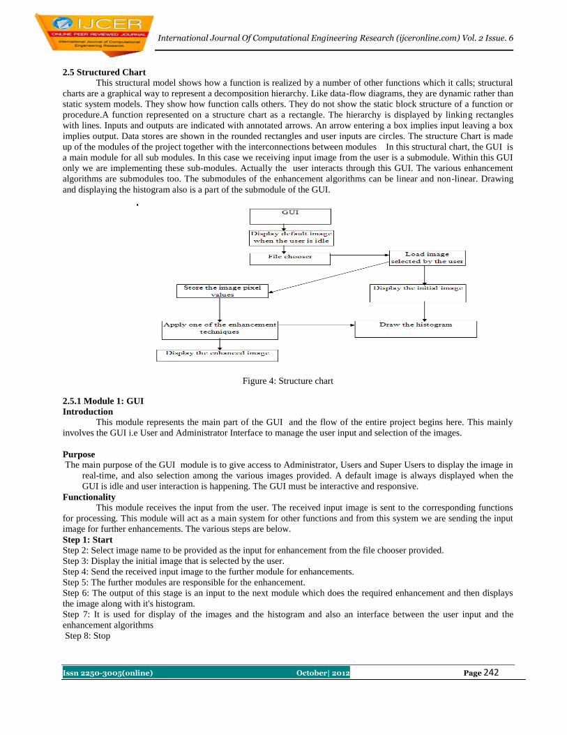
International Journal Of Computational Engineering Research (ijceronline.com) Vol. 2 Issue. 6
Issn 2250-3005(online) October| 2012 Page 242
2.5 Structured Chart
This structural model shows how a function is realized by a number of other functions which it calls; structural
charts are a graphical way to represent a decomposition hierarchy. Like data-flow diagrams, they are dynamic rather than
static system models. They show how function calls others. They do not show the static block structure of a function or
procedure.A function represented on a structure chart as a rectangle. The hierarchy is displayed by linking rectangles
with lines. Inputs and outputs are indicated with annotated arrows. An arrow entering a box implies input leaving a box
implies output. Data stores are shown in the rounded rectangles and user inputs are circles. The structure Chart is made
up of the modules of the project together with the interconnections between modules In this structural chart, the GUI is
a main module for all sub modules. In this case we receiving input image from the user is a submodule. Within this GUI
only we are implementing these sub-modules. Actually the user interacts through this GUI. The various enhancement
algorithms are submodules too. The submodules of the enhancement algorithms can be linear and non-linear. Drawing
and displaying the histogram also is a part of the submodule of the GUI.
Figure 4: Structure chart
2.5.1 Module 1: GUI
Introduction
This module represents the main part of the GUI and the flow of the entire project begins here. This mainly
involves the GUI i.e User and Administrator Interface to manage the user input and selection of the images.
Purpose
The main purpose of the GUI module is to give access to Administrator, Users and Super Users to display the image in
real-time, and also selection among the various images provided. A default image is always displayed when the
GUI is idle and user interaction is happening. The GUI must be interactive and responsive.
Functionality
This module receives the input from the user. The received input image is sent to the corresponding functions
for processing. This module will act as a main system for other functions and from this system we are sending the input
image for further enhancements. The various steps are below.
Step 1: Start
Step 2: Select image name to be provided as the input for enhancement from the file chooser provided.
Step 3: Display the initial image that is selected by the user.
Step 4: Send the received input image to the further module for enhancements.
Step 5: The further modules are responsible for the enhancement.
Step 6: The output of this stage is an input to the next module which does the required enhancement and then displays
the image along with it's histogram.
Step 7: It is used for display of the images and the histogram and also an interface between the user input and the
enhancement algorithms
Step 8: Stop

International Journal Of Computational Engineering Research (ijceronline.com) Vol. 2 Issue. 6
Issn 2250-3005(online) October| 2012 Page 243
Input
This module accepts the inputs from the user in the form of the image selected from the file chooser.
Output
This module send the selected image to the further modules for enhancement.
Inter component Relationship
This module receives inputs from the user which is received by subsequent modules for further enhancements and
display.
2.5.2 Module 2: Input image Retrieval
Introduction
The particular image input have to be retrieved from the GUI where the user interacts. The module is
responsible for checking whether the image retrieved as per the specifications(fixed image).
Purpose
This module will be responsible for getting inputs from user for retrieving data and report it to display module.
Functionality
This module accepts input from user through the GUI.
The various steps are as below.
Step 1: Start
Step 2: Select a file name which contains the input image.
Step 3: Display the initial image.
Step 4: Grab the pixel values of the input image and store it in a buffer for modification during enhancement.
Step 5: Send the retrieved input to the Display module through the main GUI for different displays.
Step 6: If we want retrieve pixel values for another input image than go to Step 2 otherwise go to Step 7
Step 7: Stop
Input
This module accepts input from the user as an image and sends it for displaying and drawing of the histogram.
Output
This module returns the enhanced image as the output.
Inter component Relationship
This retrieves the input from the user and produces the retrieved inputs as an output to the Display module
through the GUI.
2.5.3 Module 3: Image Display
Introduction
In image display, the particular image to be enhanced must be retrieved and based on the pixel values stored,
the image is appropriately drawn. There are various inbuilt functions for drawing the image from the pixel values. The
appropriate packages must be imported. The histogram for the image must also be displayed.
Purpose
The main purpose of the image Display module is to display the initial and final image after enhancement.
Functionality
his module accepts inputs as pixel values from the buffer where it is stored. Based on the value of the pixels,
the image is drawn onto the display. The pixel values determine the resolution of the image being displayed.
Steps:
The various steps are as below:
Step 1: Start
Step 2: Select the image name for display
Step 3: Select the image format for display
Step 4: Start to receive pixel data from the buffer and start drawing the image onto the screen.

International Journal Of Computational Engineering Research (ijceronline.com) Vol. 2 Issue. 6
Issn 2250-3005(online) October| 2012 Page 244
Step 5: Display the image in the required proper format.
Step 6: Send the display details to Display_Mode module for different displays.
Step 7: Stop
Input
This module accepts the input data as the pixel values of the input image which is stored in the buffer..
Output This module returns the pixel data that is raw data display to Display_Mode.
Inter component Relationship
This function receives input from the Retrieval module to produce the image and histogram display as output. That
displayed output send to Display_Mode module.
2.5.4 Module 4: Histogram display Mode[10]
Introduction
Already we know about full frame mode display in where both the initial and final images are displayed
together along with their histogram respectively.
Purpose
This module is responsible for the displaying only selected single frame from the master frame either only the
image or the histogram.
Functionality
This module is responsible to displaying selected single frame and drawing the histogram. JfreeChart is used to
plot the graph by taking pixel values as the input.
The steps are as below.
Step 1: Start
Step 2: Make sure that the appropriate libraries are included that the JfreeChart requires for plotting the histogram.
Step 3: The pixel values of the image for which the histogram is to be drawn are pass to the JFreeChart.
Step 4: Then it reads these pixel values and plots the graph.
Step 5: The histogram is displayed for the image selected.
Step 6: Stop
Input
It receives pixel values from the image for which the histogram is to be plotted.
Output
The graphical representation of the intensity of the image by drawing the histogram for the image selected by the user.
Inter component Relationship
It mainly depends on the intensity of the pixels of the image selected. Depending on pixel values, a smooth or sharp or
dense or exponential or linear or non-linear curve may be obtained.
2.5.5 Module 5: Stepwise Linear stretching
Introduction
This is an enhancement algorithm which takes the input image given by the user and enhances the image and
displays it along with it's histogram.
Purpose
This module is responsible for stretching the pixel values so that the image intensity becomes more uniform.
Functionality
This module is responsible to displaying the selected image and compare it before and after enhancement . The
various steps are as below.
Step 1: Start
Step 2: The image to be enhanced is selected by the user and the pixel values are grabbed.
Step 3: The pixel values of the initial image are not uniform. The intensity is high at the peaks. All the pixel values at
peaks are stretched so that the histogram curve becomes smooth and uniform.

International Journal Of Computational Engineering Research (ijceronline.com) Vol. 2 Issue. 6
Issn 2250-3005(online) October| 2012 Page 245
Step 4: The modified pixel values are then used to draw the enhanced image.
Step 5: This image is now sent to the display module.
Step 6: Stop
Input
It receives pixel values grabbed from the selected input image.
Output
The selected input image is modified and the final image is displayed along with the histogram.
Inter component Relationship
It mainly depends on the pixel values of the input image and the intensity curve distribution.
2.5.6 Module 6: Linear equalization[11]
Introduction
This is an enhancement algorithm which takes the input image given by the user and enhances the image and
displays it along with it's histogram.
Purpose
This module is responsible for equalizing the pixel values so that the image intensity becomes more uniform and is
equally distributed.
Functionality
This module is responsible to displaying the selected image and compare it before and after enhancement . The
various steps are as below.
Step 1: Start
Step 2: The image to be enhanced is selected by the user and the pixel values are grabbed.
Step 3: The pixel values of the initial image are not uniform. The intensity is high at the peaks.
Step 4: The maximum and minimum values of the occurances of the image pixel values are identified
and the value less than minimum is considered as zero and the value greater than maximum is 255.
Step 5: The modified pixel values are then used to draw the enhanced image.
Step 6: This image is now sent to the display module.
Step 7: Stop
Input
It receives pixel values grabbed from the selected input image.
The selected input image is modified and the final image is displayed along with the histogram.
Inter component Relationship
It mainly depends on the pixel values of the input image and the intensity curve distribution.
2.5.7 Module 7: Modification of the resolution
Introduction
This is a modification technique which takes the input image given by the user and enhances the image and
displays both the images onto the frame.
Purpose
This module is responsible for modifying the pixel values so that the image intensity becomes as desired by the user.
Functionality
This module is responsible to displaying the selected image and compare it before and after modification . The various
steps are as below.
Step 1: Start
Step 2: The image to be modified is selected by the user and the pixel values are grabbed.
Step 3: The pixel values of the initial image are not uniform.
Step 4: It contains six options:
3. Brightness
4. Darkness
5. Edge detection
6. Negative

International Journal Of Computational Engineering Research (ijceronline.com) Vol. 2 Issue. 6
Issn 2250-3005(online) October| 2012 Page 246
7. Reset
Step 5: Based on the option selected, the pixel values are modifie
Brightness is used to increase the resolution of the pixels so that it looks more bright where as darkness does
the opposite of this function. Negative nverts the value of each and every pixel value. Reset is used to get back
the itial image after applying one of these modification techniques so that the next modification can be
applied later.
Step 6: The modified pixel values are then used to draw the enhanced image.
Step 7: This image is now sent to the display module.
Step 8: Stop
Input
It receives pixel values grabbed from the selected input image.
Output
The selected input image is modified and the final image is displayed. The initial image can be got back by clicking on
the reset option.
Inter component Relationship
It mainly depends on the pixel values of the input image and the resolution of the pixel values of the image being used.
2.5.8 Module 8: Global Histogram equalization[11]
Introduction
This is an enhancement algorithm which takes the input image given by the user and enhances the image globally and
displays both the initial and final images.
Purpose
This module is responsible for equalizing the pixel values so that the image intensity becomes more uniform and is
equally distributed. This is based on the global values of the pixels
Functionality
This module is responsible to displaying the selected image and compare it before and after enhancement . The various
steps are as below.
Step 1: Start
Step 2: The image to be enhanced is selected by the user and the pixel values are rabbed.
Step 3: The pixel values of the initial image are not uniform.
Step 4: The pixel values of the image to be enhanced are used to get the RGB (Red Green Blue) components. Using this,
the HSV(Hue Saturation Value)
components of the image are obtained. The hue and saturation remain the
same,where as the value is modified to enhance the image intensity. Then the
modified value is used and the new HSV values are converted back into their
corresponding RGB values and this value of pixels are used to draw the
enhanced image.
Step 5: The modified and enhanced pixel values are then used to draw the enhanced image.
Step 6: This image is now sent to the display module.
Step 7: Stop
Input
It receives pixel values grabbed from the selected input image.
Output
The selected input image is globally equalized based on the RGB values of the pixels and the final image is
displayed along with the histogram.
Inter component Relationship
It mainly depends on the pixel values of the input image and the intensity curve distribution and mainly on the RGB
values and the corresponding HSV values.
2.5.9 Module 9: Scaling and shearing of images
Introduction
This is a processing algorithm which takes the input image given by the user and modifies the imagefor scaling
and shearing[12] effects and displays both the initial and final images.

International Journal Of Computational Engineering Research (ijceronline.com) Vol. 2 Issue. 6
Issn 2250-3005(online) October| 2012 Page 247
Purpose
This module is responsible for modifying the pixel values so that the image intensity becomes as desired by the user.
Functionality
This module is responsible to displaying the selected image and compare it before and after enhancement . The various
steps are as below.
Step 1: Start
Step 2: The image to be enhanced is selected by the user and the pixel values are grabbed.
Step 3: The pixel values of the initial image are not uniform.
Step 4: If it is scale value then matrix becomes
[sx 0 0] sx-The factor by which the co ordinate are scaled along x axis
direction.
[0 sy 0] sy-The factor by which the co ordinate are scaled along y axis
direction.
If it is shear value matrix becomes
[1 shx 0] shx-Multiplier by which co-ordinates are shifted in the direction of
+ve X axis as factor of their y co-ordinates.
[shy 1 0] shy- Multiplier by which co-ordinates are shifted in the direction of +ve Y axis as factor of their X co-
ordinates.
Step 5: Draw the processed image on buffer using graphics function.
The modified and enhanced pixel values are then used to draw the enhanced image.
Step 6: This image is now sent to the display module.
Step 7: Stop
Input
It receives pixel values grabbed from the selected input image.
Output
The selected input image is modified and the final image is displayed. The initial image can be displayed again
and compared with the final image..
Inter component Relationship
It mainly depends on the pixel values of the input image and the resolution of the pixel values of the image being used.
2.5.10 Module 10: Filters
Introduction
This is a processing algorithm which takes the input image given by the user and modifies the image for scaling
and shearing effects and displays both the initial and final images.
Purpose
This module is responsible for modifying the pixel values so that the image intensity becomes as desired by the user.
Functionality
This module is responsible to displaying the selected image and compare it before and after enhancement . The various
steps are as below.
Step 1: Start
Step 2: The image to be enhanced is selected by the user and the pixel values are grabbed.
Step 3: The pixel values of the initial image are not uniform.
Step 4: Here we are doing three kinds of filters, blue, green and red. In green filter,
we consider the RGB color matrix and in that we make only the value of
green as 1 and the others 0. Similarly for red and blue.
Step 5: The modified and enhanced pixel values are then used to draw the enhanced image.
Step 6: This image is now sent to the display module.
Step 7: Stop
Input
It receives pixel values grabbed from the selected input image.
Output
The selected input image is modified and the final image is displayed. The initial image can be displayed again and
compared with the final image..
Inter component RelationshipIt mainly depends on the pixel values of the input image and the resolution of the pixel
values of the image being used.

International Journal Of Computational Engineering Research (ijceronline.com) Vol. 2 Issue. 6
Issn 2250-3005(online) October| 2012 Page 248
3. TESTING: Test Cases for Unit Testing:
Module under test Image retrieval
Description Retrieving the pixel values from the input image
Sample input fish.jpg
Expected output It should store the pixel values of this image
Actual output The pixel values of the input image are stored
Remarks Test is successful
Module under test Image display
Description Display the images in the required format
Sample input fish.jpg
Expected output It should display the initial and final image in the required
fashion and format
Actual output The initial and final images are displayed as required
Remarks Test is successful
Module under test Histogram display
Description Display the histogram for the initial and final images
Sample input fish.jpg
Expected output It should draw the histogram based on the pixel values
passed to the JFreeChart
Actual output The histogram is drawn and displayed
Remarks Test is successful
Module under test Stepwise linear stretching
Description It equalizes the pixel values by stretching the values present at
the peak
Sample input fish.jpg
Expected output The enhanced image along with the histogram
Actual output The enhanced image is displayed
Remarks Test is successful
Module under test Linear equalization
Description It equalizes the pixel values by finding the minimum and
maximum occurances of the pixel values
Sample input fish.jpg
Expected output The enhanced image along with the histogram
Actual output The enhanced image is displayed
Remarks Test is successful

International Journal Of Computational Engineering Research (ijceronline.com) Vol. 2 Issue. 6
Issn 2250-3005(online) October| 2012 Page 249
Module under test Modification of resolution
Description It modifies the pixel values either brighten or darken or
form the negative or contrast
Sample input fish.jpg
Expected output The enhanced image must be displayed
Actual output The enhanced image is displayed
Remarks Test is successful
Module under test Global Histogram equalization
Description It equalizes the pixel values globally by converting the RGB
values to HSV. Then the value is enhanced and converted
back to RGB
Sample input fish.jpg
Expected output The enhanced image along with the histogram
Actual output The enhanced image is displayed
Remarks Test is successful
Module under test Scaling and Shearing images
Description It scales or shears the input image by a given value along the x
or y axis according to a matrix. The modified pixel values are
used to draw the final image.
Sample input fish.jpg
Expected output The modified image along with the histogram
Actual output The modified image is displayed
Remarks Test is successful
Module under test Filters
Description It uses three different filters blue, green and red. A matrix is
used for modification of the pixel values. These modified
pixel values are used for the final output.
Sample input fish.jpg
Expected output The modified image along with the histogram
Actual output The modified image is displayed
Remarks Test is successful
4. SCREEN SHOTS
Run the Main program.
We will get the intial image and its histogram.

International Journal Of Computational Engineering Research (ijceronline.com) Vol. 2 Issue. 6
Issn 2250-3005(online) October| 2012 Page 250
Initial image and its histogram.
Choose the option Stepwise Linear Equalization.
We shall get intial as well as enhanced images along with their histograms.
Stepwise Linear Equalization of the image and its histogram.
Choose the option Globalhistogram.
We shall get the enhanced image along with its histogram.
Global Histogram Equalization of the image and its histogram.
Choose the option Linear Equalization.
We shall get the enhanced image along with its histogram.
Linear Equalization of image and its histogram.
Choose the option Modification of Resolution.
We shall get options to modify the Brightness, Darkness, Contrast and Negative of images.

International Journal Of Computational Engineering Research (ijceronline.com) Vol. 2 Issue. 6
Issn 2250-3005(online) October| 2012 Page 251
a. Brightness of image b. Darkness of image
c. Contrast of image d. Negative of image
5. CONCLUSION AND FUTURE ENHANCEMENTS
Conclusions
The application deals with the retrieval of pixel values from the selected user image and applying one of the
image enhancement algorithm. Then it displays the histogram. The major portion of the project is concentrated on
“JAVA” on Linux platform. Various options are provided to implement one of the enhancement algorithm. These
include stepwise linear stretching, linear equalization, global histogram equalization, modification of resolution.
The user selects one of the best-suited distribution algorithm for the image selected. The histogram is drawn for
both the initial image and the final image. After enhancement, the histogram curve becomes smoother. The application is
made interactive by allowing the user to select the image to be enhanced.
Limitations
The limitations of the product are not negative aspects of the work done. However, no product can fulfill all the
needs of the user. With respect to this, the following might be the limitations of this package.
Some important limitations are as follows:
1. The package has been designed for only fixed images.
2. The application includes only a few of the algorithms for enhancement and does not cover all possible
algorithms.
3. Few vulnerabilities associated with the Linux Operating system are as mentioned below:
3.1 Superuser may misuse the privileges granted to him.
3.2 Many system files can be changed easily
3.3 Modules can be easily used to intercept the kernel.
Future enhancements
The software can be extended to support the following functionality:
This application will be supported on Linux platform as well as windows operating system.
This application, which currently supports fixed images can be extended for moving images such as videos and also
for satellite images which are in the form of raw binary data.
Color histograms can also be implemented along with intensity histogram.

International Journal Of Computational Engineering Research (ijceronline.com) Vol. 2 Issue. 6
Issn 2250-3005(online) October| 2012 Page 252
References [1]. Java: The complete reference, Seventh Edition, Herbert Schildt, Tata McGraw Publishing Company Limited.
[2]. Digital Image Processing-Concepts, Algorithms, and Scientific Applications, Jaehne. B, Springer, Berlin 1991
[3]. Digital Image Processing, Third Edition, Rafael. C. Gonzalez and Richard. E. Woods, Prentice Hall 2002
[4]. The image processing handbook, Fifth edition, John. C. Russ, IEEE Press, New York 1994
[5]. Digital Image Processing: Principles and Applications, Baxes.G.A., Wiley, New York 1994
[6]. Digital Image Processing, Gonzalez.R.C. and Wintz.P.A, Addison-Wesley 1977
[7]. An Introduction to Digital Image Processing, Niblack.W., Prentice Hall 1986
[8]. http://en.wikipedia.org/wiki/Digital_image_processing
[9]. http://www.cromwell-intl.com/3d/histogram
[10]. http://designer-info.com/Writing/image_enhancement.htm
[11]. http://en.wikipedia.org/wiki/Histogram_equalization
[12]. http:/en.wikipedia.org/wiki/Color_model

International Journal Of Computational Engineering Research (ijceronline.com) Vol. 2 Issue. 6
Issn 2250-3005(online) October| 2012 Page 253
Analyzing & Identifying The Superlative Keying Protocol To Support
Sensor Networking
Akula Santha Manohari1, Ravi Kumar. Singisetti
2
1,M.Tech Student(Neural Networks), Gokul institute of Engineering & Technology, Piridi,Bobilli
2,Asst.Professor, Gokul institute of Engineering & Technology, Piridi,Bobilli.
Abstract The sensor networks like mobile sensor networks or the network that are built in a hurry are deployed in whimsical
and undersigned configuration. For this reason, the sensor in such a network may become eventually adjacent to any other
sensor in the network. In order to make a communication between every pair of adjacent sensors, in a secure way in such an
arbitrary network, each sensor ,let x in the network be in need to store n-1 symmetric keys that sensor x shares with all the
other sensors where n is the number that represents the count of the sensors in the network. When the number n is large and if
the availability of storage in each sensor is reserved, then the storage requirement for the keying protocol is a bit hard. Some
earlier achievements were made just to redesign this keying protocol and also to reduce the number of keys to be stored in
each sensor .Those achievements have exhibited protocols that are accessible to collusion attacks, eavesdropping, and
impersonation. We want to present a secure keying protocol that makes each sensor to store (n+1)/2 keys that are less that n-1
keys that are needed to be stored in each sensor in the original keying protocol. In this paper we also want to show that each
sensor needs to store at least (n-1)/2 keys, in any of the fully secure keying protocol.
I. Introduction A wireless sensor network (WSN) consists of spatially distributed autonomous sensors to monitor physical or
environmental conditions, such as temperature, sound, pressure, etc. and to cooperatively pass their data through the network to
a main location.
Fig.1: Wireless Sensor Network
Many wireless sensor networks are deployed in random and unintended style. Examples of such networks are
networks of mobile sensors [11] and networks that are deployed in a hurry to monitor evolving crisis situations [7] or
continuously changing battle fields [1]. In any such network, any deployed sensor can end up being adjacent to any other
deployed sensor. Thus, each pair of sensors, say sensors x and y, in the network need to share a symmetric key, denoted Kx,y,
that can be used to secure the communication between sensors x and y if these two sensors happen to be deployed adjacent to
one another. In particular, if sensors x and y become adjacent to one another, then these two sensors can use their shared
symmetric key Kx,y to authenticate one another (i.e. defend against impersonation) and to encrypt and decrypt their exchanged
data messages (i.e. defend against eavesdropping).

International Journal Of Computational Engineering Research (ijceronline.com) Vol. 2 Issue. 6
Issn 2250-3005(online) October| 2012 Page 254
The probabilistic keying protocol and grid keying protocol are two main keying protocols that were proposed in the
past to reduce the number of stored keys in each sensor in the network.Unfortunately, the probabilistic keying protocol suffers
from the following problem. The stored keys in any sensor x are independent of the identity of sensor x and so these keys
cannot be used to authenticate sensor x to any other sensor in the network. In other word, the probabilistic protocol cannot
defend against impersonation.In the grid keying protocol [8], each sensor is assigned an identifier which is the coordinates of a
distinct node in a two-dimensional grid. Unfortunately, it turns out that the grid keying protocol is vulnerable to collusion.
Specifically, a small gang of adversarial sensors in the network can pool their stored keys together and use the pooled keys to
decrypt all the exchanged data messages in the sensor network.
2. CHALLENGES FOR SENSOR NETWORKS
As a third example, if the deployed sensor network is mobile, then a detailed plan of the initial topology may be of
little value.) In this network, when a sensor x is deployed, it first attempts to identify the identity of each sensor adjacent to x,
then starts to exchange data with each of those adjacent sensors. Any sensor z in this network can be an “adversary”, and can
attempt to disrupt the communication between any two legitimate sensors, say sensors x and y, by launching the following two
attacks:
a)Impersonation Attack:
Sensor z notices that it is adjacent to sensor x while sensor y is not. Thus, sensor z attempts to convince sensor x that it
(z) is in fact sensor y. If sensor z succeeds, then sensor x may start to exchange data messages with sensor z, thinking that it is
communicating with sensor y.
b)Eavesdropping Attack:
Sensor z notices that it is adjacent to both sensors x and y, and that sensors x and y are adjacent to one another. Thus,
when sensors x and y start to exchange data messages, sensor z can copy each exchanged data message between x and y.If the
network has n sensors, then each sensor in the network needs to store (n-1) symmetric keys before the network is deployed. If n
is large, then the storage requirement, just to store the required shared keys, is relatively large, especially since the size of
storage in each sensor is typically small.
To solve this problem, we present the following two results in this paper:
i) Efficiency:There is a keying protocol, where each sensor shares a distinct symmetric key with every other sensor in the
network, and yet each sensor needs to store exactly (n+1)/2 symmetric keys, before the network is deployed.
ii) Optimality:In every keying protocol, where each sensor shares a distinct symmetric key with every other sensor in the
network, each sensor needs to store at least (n-1)/2 symmetric keys, before the network is deployed.
3. PROPOSED PROTOCOL KEYING CONCEPTS & ALGORITHMS
1) Mutual Authentication: Sensor x authenticates sensor y, and sensor y authenticates sensor x.
2) Confidential Data Exchange: Encrypt and later decrypt all the exchanged data messages between x and y.
Where n denote the number of sensors in our network. Without loss of generality, we assume that n is an odd positive integer.
Each sensor in the network has a unique identifier in the range 0…n - 1. We use ix and iy to denote the identifiers of sensors x
and y, respectively, in this network. Each two sensors, say sensors x and y, share a symmetric key denoted Kx,y or Ky,x. Only the
two sensors x and y know their shared key Kx,y. And if sensors x and y ever become neighbors in the network, then they can use
their shared symmetric key Kx,y to perform above two protocol keying concepts.
Mutual Authentication Protocol:
Before the sensors are deployed in a network, each sensor x is supplied with the following items:
1) One distinct identifier ix in the range 0...n-1
2) One universal key ux
3) (n-1)/2 symmetric keys Kx,y = H(ix/uy) each of which is shared between sensor x and another sensor y, where ix is below iy.
After every sensor is supplied with these items, the sensors are deployed in random locations in the network. Now if two
sensors x and y happen to become adjacent to one another, then these two sensors need to execute a mutual authentication

International Journal Of Computational Engineering Research (ijceronline.com) Vol. 2 Issue. 6
Issn 2250-3005(online) October| 2012 Page 255
protocol so that sensor x proves to sensor y that it is indeed sensor x and sensor y proves to sensor x that it is indeed
sensor y. The mutual authentication protocol consists of the following six steps.
Step 1: Sensor x selects a random nonce nx and sends a hello message that is received by sensor y.
Step 2: Sensor y selects a random nonce ny and sends a hello message that is received by sensor x.
Step 3: Sensor x determines whether ix is below iy. Then it either fetches Kx;y from its memory or computes it. Finally, sensor
x sends a verify message to sensor y.
Step 4: Sensor y determines whether iy is below ix. Then it either fetches Kx;y from its memory or computes it. Finally, sensor
y sends a verify message to sensor x.
Step 5: Sensor x computes H(ix|iy|ny|Kx,y) and compares it with the received H(ix|iy|ny|Kx,y). If they are equal, then x
concludes that the sensor claiming to be sensor y is indeed sensor y. Otherwise, no conclusion can be reached.
Step 6: Sensor y computes H(ix|iy|ny|Kx,y) and compares it with the received H(ix|iy|ny|Kx,y). If they are equal, then y
concludes that the sensor claiming to be sensor x is indeed sensor x. Otherwise, no conclusion can be reached.
Data Exchange Protocol:
After two adjacent sensors x and y have authenticated one another using the mutual authentication protocol described
in the previous section, sensors x and y can now start exchanging data messages according to the following data exchange
protocol. (Recall that nx and ny are the two nonces that were selected at random by sensors x and y, respectively, in the mutual
authentication protocol.)
Step 1: Sensor x concatenates the nonce ny with the text of the data message to be sent, encrypts the concatenation using the
symmetric key Kx;y, and sends the result in a data message to sensor y.
Step 2: Sensor y concatenates the nonce nx with the text of the data message to be sent, encrypts the concatenation using the
symmetric key Kx;y, and sends the result in a data message to sensor x.
4. DESIGN & IMPLEMENTATION OF THE SYSTEM Design is concerned with identifying software components specifying relationships among components. Specifying software
structure and providing blue print for the document phase. Modularity is one of the desirable properties of large systems. It
implies that the system is divided into several parts. In such a manner, the interaction between parts is minimal clearly
specified. Design will explain software components in detail. This will help the implementation of the system. Moreover, this
will guide the further changes in the system to satisfy the future requirements.
Class Diagram contains the following elements:
A class which represents entities with common characteristics or features attributes operations and associations.
Association, which represent relationship between two or more classes where relationships have common characteristics or
features like attributes and operations as in Fig.2.

International Journal Of Computational Engineering Research (ijceronline.com) Vol. 2 Issue. 6
Issn 2250-3005(online) October| 2012 Page 256
Fig 2: Inter-operational Class diagram for framework
Fig 3: Inter-operational Sequence diagram for the Server & sensors
Sequence Diagrams represents the interactions between classes to achieve a result such as a usecase. The sequence diagram lists
objects horizontally and time vertically, and models these messages over time. In this paper the designing of the sequence has
been done on both server and the sensors and they were described as in the Fig.3
5. RESULTS The below are the results obtained
Fig.4: Receiver 0 Communication
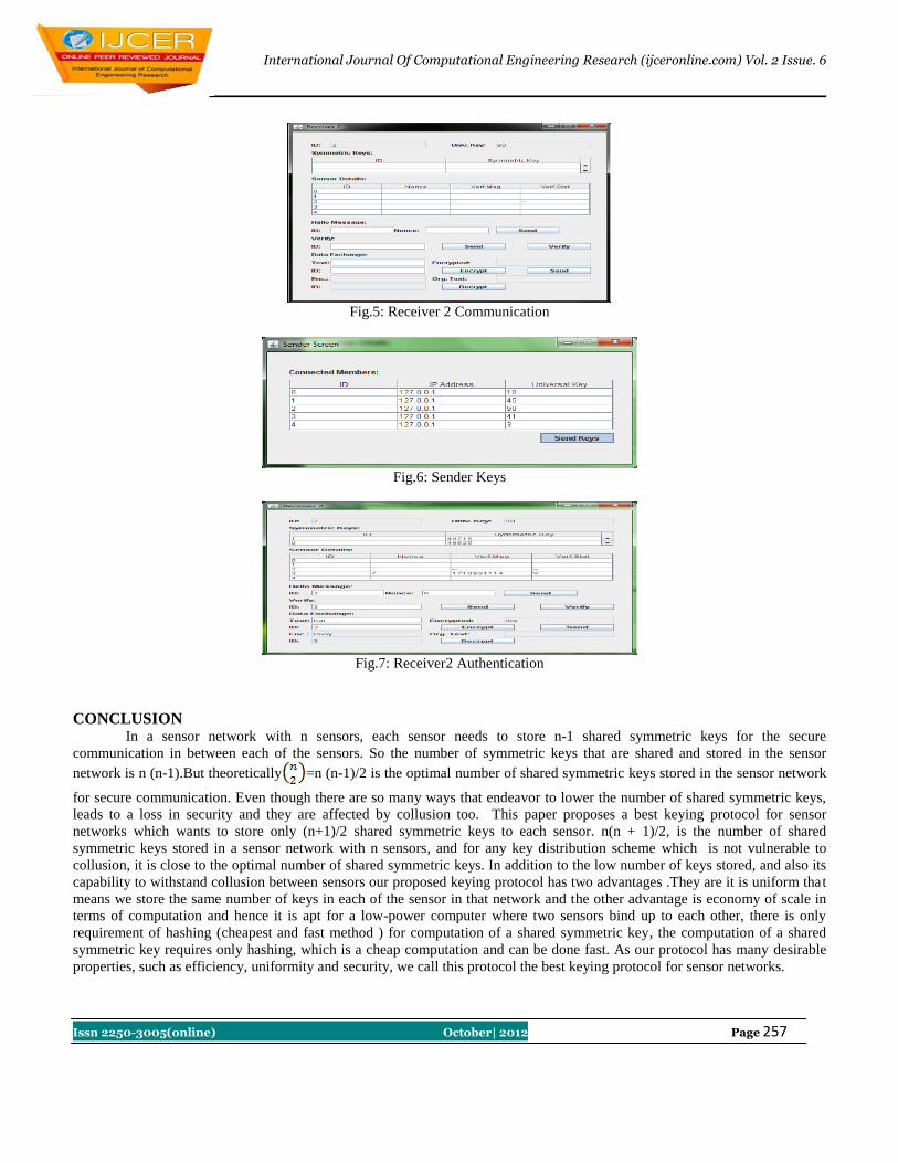
International Journal Of Computational Engineering Research (ijceronline.com) Vol. 2 Issue. 6
Issn 2250-3005(online) October| 2012 Page 257
Fig.5: Receiver 2 Communication
Fig.6: Sender Keys
Fig.7: Receiver2 Authentication
CONCLUSION
In a sensor network with n sensors, each sensor needs to store n-1 shared symmetric keys for the secure
communication in between each of the sensors. So the number of symmetric keys that are shared and stored in the sensor
network is n (n-1).But theoretically =n (n-1)/2 is the optimal number of shared symmetric keys stored in the sensor network
for secure communication. Even though there are so many ways that endeavor to lower the number of shared symmetric keys,
leads to a loss in security and they are affected by collusion too. This paper proposes a best keying protocol for sensor
networks which wants to store only (n+1)/2 shared symmetric keys to each sensor. n(n + 1)/2, is the number of shared
symmetric keys stored in a sensor network with n sensors, and for any key distribution scheme which is not vulnerable to
collusion, it is close to the optimal number of shared symmetric keys. In addition to the low number of keys stored, and also its
capability to withstand collusion between sensors our proposed keying protocol has two advantages .They are it is uniform that
means we store the same number of keys in each of the sensor in that network and the other advantage is economy of scale in
terms of computation and hence it is apt for a low-power computer where two sensors bind up to each other, there is only
requirement of hashing (cheapest and fast method ) for computation of a shared symmetric key, the computation of a shared
symmetric key requires only hashing, which is a cheap computation and can be done fast. As our protocol has many desirable
properties, such as efficiency, uniformity and security, we call this protocol the best keying protocol for sensor networks.

International Journal Of Computational Engineering Research (ijceronline.com) Vol. 2 Issue. 6
Issn 2250-3005(online) October| 2012 Page 258
References [1] S. Sana and M. Matsumoto, “Proceedings of a wireless sensor network protocol for disaster management,” in
Information, Decision and Control (IDC), 2007, pp. 209 –213.
[2] S. Hynes and N. C. Rowe, “A multi-agent simulation for assessing massive sensor deployment,” Journal of Battlefield
Technology, vol. 7, pp. 23–36, 2004.
[3] S. S. Kulkarni, M. G. Gouda, and A. Arora, “Secret instantiation in ad-hoc networks,” Special Issue of Elsevier Journal
of Computer Communications on Dependable Wireless Sensor Networks, vol. 29, pp. 200–215, 2005.
[4] A. Aiyer, L. Alvisi, and M. Gouda, “Key grids: A protocol family for assigning symmetric keys,” in Proceedings of
IEEE International Conference on Network Protocols (ICNP), 2006, pp. 178–186.
[5] A. Howard, M. J. Mataric, and G. S. Sukhatme, “Mobile sensor network deployment using potential fields: A
distributed, scalable solution to the area coverage problem,” in Proceedings of the International Symposium on
Distributed Autonomous Robotic Systems (DARS), 2002, pp. 299–308.
[6] Y. Fan and J. S. Thompson, “MIMO Configurations for Relay Channels: Theory and Practice,” IEEE Trans. on Wireless
Communications, Vol. 6, Issue 5, pp. 1774-1786, May 2007.
[7] A. Bletsas, A. Khisti, D. P. Reed, and A. Lippman, “A Simple Cooperative Diversity Method Based on Network Path
Selection,” IEEE Journal on Selected Areas in Communications, Vol. 24, Issue 3, pp. 659-672, Mar. 2006.
[8] A. Host-Madsen, “Capacity Bounds for Cooperative Diversity,” IEEE Trans. on Information Theory, Vol. 52, No. 4, pp.
1522-1544, Apr. 2006.
[9] S. Krco and M. Dupcinov, “Improved Neighbor Detection Algorithm for AODV Routing Protocol,” IEEE
Communication Letters, Vol. 7, No. 12, pp. 584-586, Dec. 2003.
[10] Intersil Prism WLAN Chipset Application Note: Tutorial on Basic Link Budget Analysis, Available from
http://www.sssmag. com/pdf/an9804.pdf, 2006.
[11] J. N. Laneman, “Cooperative Diversity in Wireless Networks: Algorithms and Architectures,” Ph.D. Thesis,
Massachusetts Institute of Technology, Cambridge, MA, Aug. 2002.
Author List:
Akula Santha Manohari received B.Tech in Computer science from JNTUH, Pursuing M.Tech in Neural
Networks from Gokul institute of Engineering & Technology Affiliated to JNTUK.. Her research area of interests are Data
mining and computer networks
Ravi Kumar. Singisetti Received B.Tech from SISTAM at Srikakulam in the year 2008 and M.Tech from GOKUL institute of
Engineering & Technology , piridi ,Bobilli.Presently Working as Ass.Professor in the Dept of CSE at institute of Engineering
& Technology.