International Journal of Chaos, Control, Modelling and ...airccse.org/journal/ijccms/papers/3214ijccms01.pdfA Comparative study of controllers for stabilizing a Rotary Inverted Pendulum

International Journal of Chaos, Control, Modelling and Simulation (IJCCMS) Vol.3, No.1/2, June 2014

DOI : 10.5121/ijccms.2014.3201 1

A Comparative study of controllers for stabilizing a

Rotary Inverted Pendulum

Velchuri Sirisha and Dr. Anjali. S. Junghare

Electrical Engineering Department, Visvesvaraya National Institute of Technology,

Nagpur, India

Abstract

This paper describes comparative study of various controllers on Rotary Inverted Pendulum (RIP). PID,

LQR, FUZZY LOGIC and H∞ controllers are tried on RIP in MatLab Simulink. The same four controllers

have been tested on test bed of RIP system the controllers are compared from various aspects. The

controllers in simulink are compared with the controllers in real time.

Keywords Fuzzy Logic, H∞, LQR, PID, RIP

1.Introduction

A typical unstable non-linear Inverted Pendulum system is often used as a benchmark to study

various control techniques in control engineering. Analysis of controllers on RIP illustrates the

analysis in cases such as control of a space booster rocket and a satellite, an automatic aircraft

landing system, aircraft stabilization in the turbulent air-flow, stabilization of a cabin in a ship etc.

RIP is a test bed for the study of various controllers like PID controller, LQR controller, and

fuzzy controller. A normal pendulum is stable when hanging downwards, an inverted pendulum

is inherently unstable, and must be actively balanced in order to remain upright, this can be done

either by applying a torque at the pivot point, by moving the pivot point horizontally as part of

a feedback system.

In this paper controllers are developed that keep the pendulum upright without any oscillations.

The model is simulated using the MATLAB application. The paper is organized as follows.

Section 2 deals with the modeling of the system, Section 3 discusses the control techniques PID,

LQR, Fuzzy Logic and H infinity controllers, Section 4 gives the test bed results, Section 5

discusses the conclusion drawn from the analysis of these controllers in simulink and on test bed.

1.Modelling of Rotary Inverted Pendulum

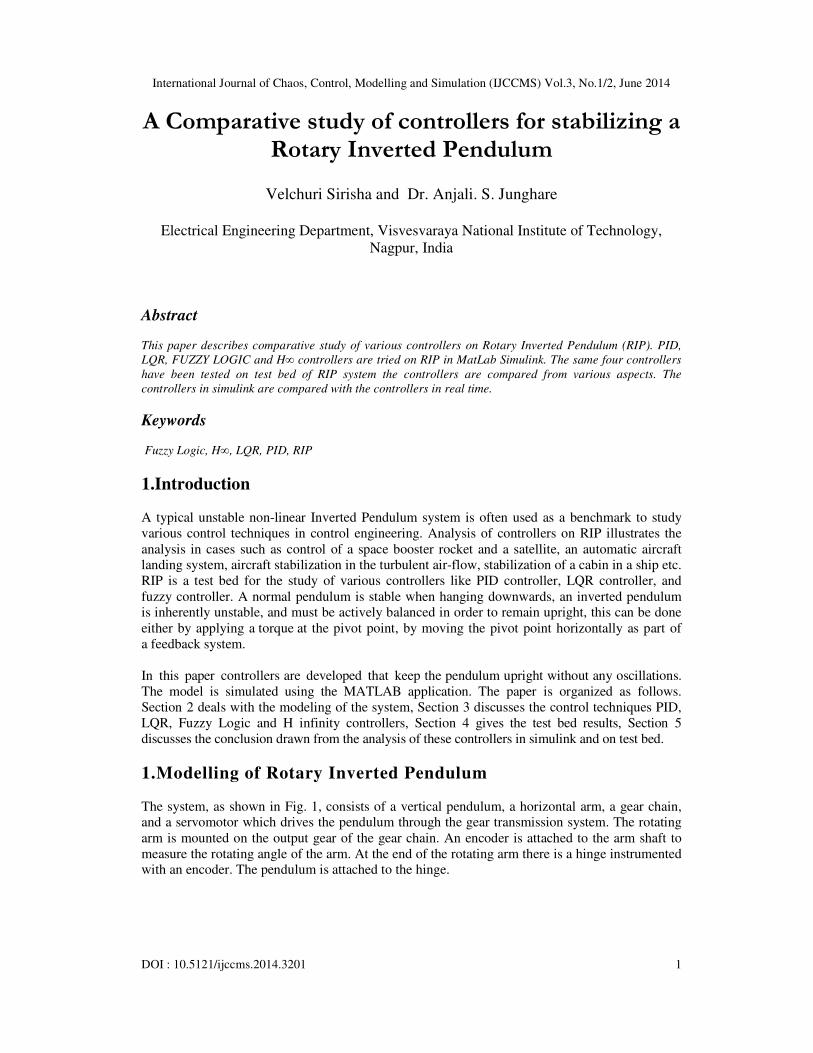
The system, as shown in Fig. 1, consists of a vertical pendulum, a horizontal arm, a gear chain,

and a servomotor which drives the pendulum through the gear transmission system. The rotating

arm is mounted on the output gear of the gear chain. An encoder is attached to the arm shaft to

measure the rotating angle of the arm. At the end of the rotating arm there is a hinge instrumented

with an encoder. The pendulum is attached to the hinge.


2

Fig.1. Rotary Inverted Pendulum system

The inverted pendulum is shown in Fig. 2, with its physical parameters α and θ are employed as

the generalized coordinates to describe the inverted pendulum system. The pendulum is displaced

with a given α while the arm rotates with an angle of θ.

.

Fig.2. Figure showing physical parameters to be measured

Using the Lagrangian method [1], the equation of Rotary Inverted Pendulum is as follows:

�� + �� + �� sin�� − �� cos��= � − �� 1� 43�� − �� cos�� − �� sin � = 0�2�

Where Torque T is given as, � =�� ! � "#$%$&'�(&

Table I

PHYSICAL PARAMETERS OF THE SYSTEM

Parameter Description Value(SI)

J Moment of inertia at the load 0.0033

m Mass of pendulum arm 0.1250

r Rotating arm length 0.2150


3

L Length to pendulum’s center of mass 0.1675

g Gravitational constant 9.81

B Viscous damping coefficient 0.0040

! Motor torque constant 0.0077 � SRV02 system gear ratio 70 � Back-EMF constant 0.0077 )� Armature resistance 2.6 �� Motor efficiency 0.69 �� Gear efficiency 0.90

Solving the equations (1), (2) and (3) and values from the Table I, state space model is formed

which is written as,

*�� + = *0 0 1 00 0 0 10 39.32 −14.52 00 81.78 −13.98 0+ *

�� + + *0025.5424.59+ 1

The state space parameters [2] are written as,

2 = *0 0 1 00 0 0 10 39.32 −14.52 00 81.78 −13.98 0+ ; � = *0025.5424.59+

C= 41 0 0 00 1 0 05; D=0;

1.Controller Design

3.1 PID Controller Proportional, integral derivative are the controllers whose output, a control variable (CV), is

generally based on the error (e) between some user-defined set point (SP) and some measured

process variable (PV).


4

Fig.3. Schematic diagram for the closed loop system with force as a disturbance

The transfer function of PID is written as [3]

�6� = 7 + 86 + 96

Manual tuning method is used to determine the gains [4].

Ki and Kd are set to zero. Then, Kp is increased until the output of the loop oscillates, after

obtaining optimum Kp value, it is set to approximately half of that value for a "quarter amplitude

decay" type response. Then, Ki is increased until any offset is corrected in sufficient time for the

process. However, too much Ki will cause instability. Finally, Kd is increased, until the loop is

acceptably quick to reach its reference after a load disturbance [5].

Fig.4. Simulink diagram of system using PID controller

Tuning the gain values Kp, Ki, Kd with 4, 2, 0.5 respectively along with a negative feedback as

shown in the simulink model of Fig.4, the position of pendulum gets stabilized as shown in Fig 5.


5

Fig.5 Variation of pendulum angle alpha (deg) with time (sec)

From Fig 5, it is observed that using PID control pendulum angle becomes zero within 1 second.

3.2 LQR Controller

LQR is a method in modern control theory that uses state-space approach to analyze a system like

inverted pendulum. The theory of optimal control is concerned with operating a dynamic

system at minimum cost. The case where system dynamics are described by a set of linear

differential equations and the cost is described by quadratic functions which are called LQ

problem [6]. The goal of such problem is to find an optimal control that minimizes a quadratic

cost functional associated with a linear system.

A system is expressed in state variable form as, :� = 2: + �;�3� The initial condition is x (0). Assuming here all the states measurable and seek to find a state-

variable feedback (SVFB) control ; = − : + < (4)

To design a SVFB that is optimal, an Index called performance index (PI) is used and is given by, � = 12= �:>?@ A: + ;>);�BC�5�

Substituting the SVFB control equation in equation (1) yields

� = 12= :>?@ �A + >) �:BC�6�

The objective in optimal design is to select the SVFB K that minimizes the performance index J.

Solving equations(3) to (6), equation (7) is obtained,

2>E + E2 + A + >) − >�>E − E� = 0 (7)

taking, = )#F�>E

it gives, 2>E + E2 + A − E�)#F�>E = 0

It is a matrix quadratic equation that is solved to get the value of auxiliary matrix P. After getting

the value of matrix P, SVFB gain K is determined.


6

Gain value is found as,

K = [-1.13 14.5 -1.44 2.46]

Fig.6 Simulink diagram of system using LQR control

By substituting the SVFB gain into the system and implemented in Simulink model of Fig.6,

system gets stabilized. Fig 7 is the response of the pendulum position of the system.

Fig. 7 Variation of pendulum position α (in deg) w.r.t time (in sec)

From Fig 7, it is observed that using LQR control, pendulum angle becomes zero within 1.5

seconds. Rotary Inverted Pendulum is stabilized at 34 degrees, and arm velocity becomes zero

within 2 seconds.

Hence, Rotary Inverted Pendulum is stable within 1.5 seconds.

3.3 Fuzzy Logic Controller (FLC)

FLC provides a simple way to arrive at a definite conclusion based upon vague, ambiguous,

imprecise, noisy, or missing input information [7]. FLC's approach to control problems mimics

how a person makes decisions. Fuzzy control describes the algorithm for process control as a

fuzzy relation between information about the condition of the process to be controlled, x and y

and the input for the process. The control algorithm is given in the IF - THEN expression such as

if x is small and y is big then z is medium.

if x is big and y is medium, then z is big.


7

The input and output variables as shown in FIS editor in Fig.8 are quantized into several modules

or fuzzy subsets and the appropriate labels are assigned in this controller [8].

Fig. 8 FIS editor with two input and one output

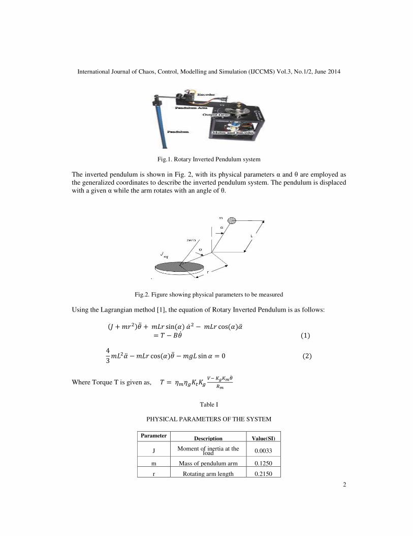
There is FLC to control pendulum angle. Five fuzzy subsets have been taken to quantize each

fuzzy variable for FLC as shown in Table II.

Table II

STANDARD LABELS OF QUANTIZATION

Linguistic Term Label

Negative big NB

Negative small NS

Zero ZE

Positive small PS

Positive big PB

Depending upon the range of alpha and alpha_dot, controlled voltage is decided. If alpha is NB

and alpha_dot is PB then according to the rule base shown in Table III, the voltage applied to the

system is zero.

Table III

FUZZY RULE BASE


8

Fig. 9 and Fig.10 shows the simulink model and simulation result of the system using fuzzy logic

controller:

Fig. 9. Simulink diagram of system for fuzzy logic controller

Fig. 10. Variation of pendulum angle with time (sec)

From results it is concluded that using fuzzy logic controller Rotary Inverted pendulum is

stabilized within 0.5 sec.

3.4 H infinity controller

In order to achieve robust performance or stabilization, the H-Infinity control method is used. The H∞ name derives from the fact that mathematically the problem may be set in the space H∞,


9

which consists of all bounded functions that are analytic in the right-half complex plane [9]. H∞

method is also used to minimize the closed loop impact of a perturbation depending on the

problem formulation the impact will be measured in terms of either stabilization or performance.

This problem is defined by the configuration of Fig 11.

Fig.11 Generalized plant

The “plant” is a given system with two inputs and two outputs. It is often referred to as the

generalized plant [9]. The signal w is an external input and represents driving signals that

generate disturbances, measurement noise, and reference inputs. The signal u is the control input.

The output z has the meaning of control error and ideally should be zero. The output y, finally, is

the observed output and is available for feedback.

The augmented plant is formed by accounting for the weighting functions W1, W2, and W3 as

shown in the Fig 12.

Fig.12. Plant with weighting functions for H∞ design

Choosing weights W1, W2 and W3 as,

W1=0.99*(s+50)/(s+.001);

W2=1;

W3=10*(s+50)/(s+500);

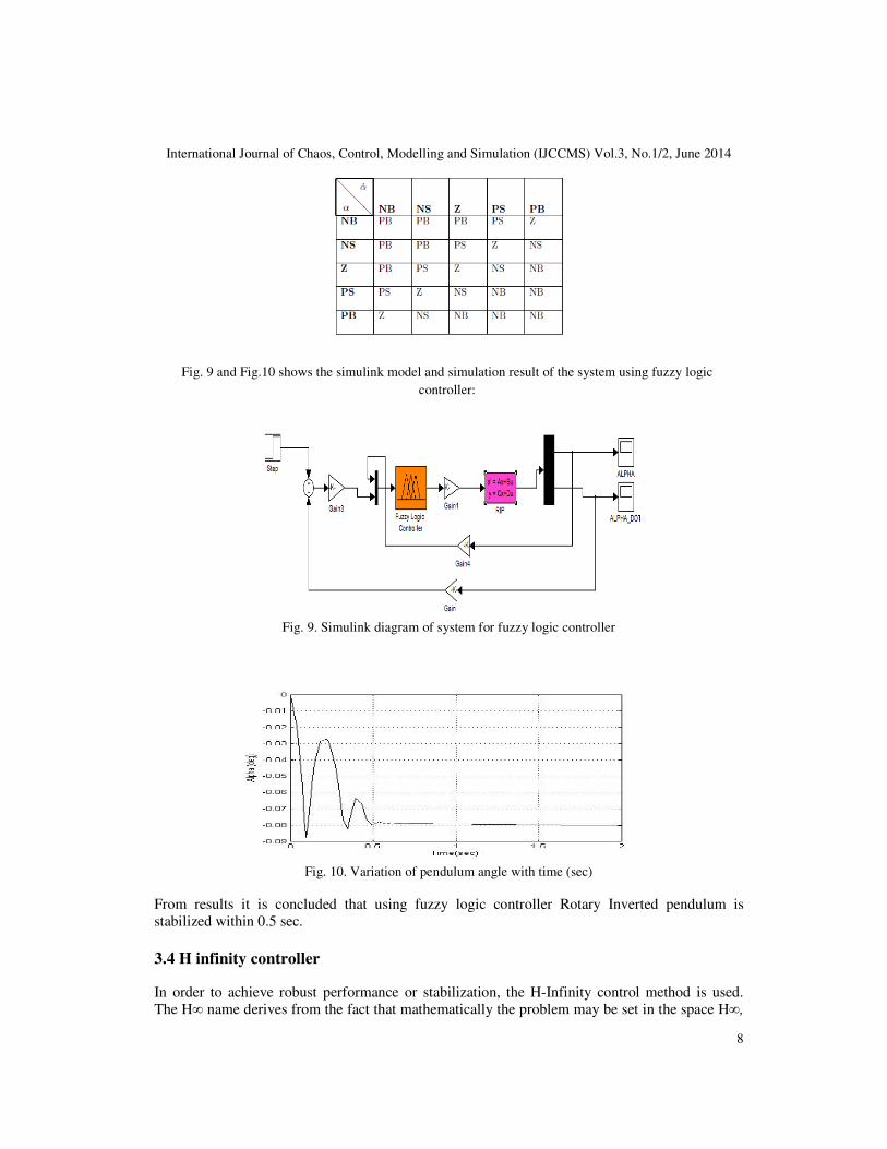
Using weights, controller in the form of state space form is obtained,


10

A =

GHHHHHHHI −0.001 0 0 0 08.356e − 025 −500 82.33 0 06.685e − 024 −3.829e − 007 −15.08 0 1−110.9 0.6872 −425.9 48.48 −84.08−106.7 0.6616 −454 46.67 −80.95KL

LLLLLLM ;

B =

GHHHHHHHI 11.11−3.961−23.69−42.23−178.7KL

LLLLLLM;

C =[−2.763 0.01 −10.92 1.57 −2];

D = [0];

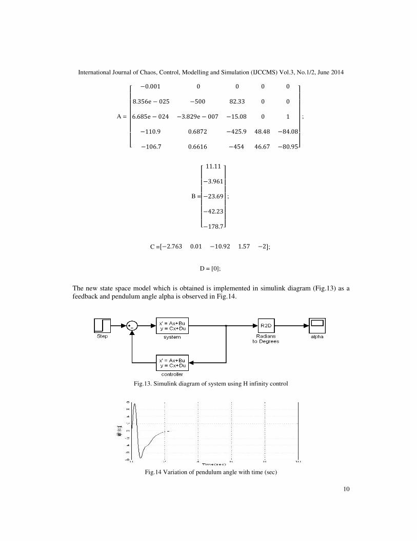
The new state space model which is obtained is implemented in simulink diagram (Fig.13) as a

feedback and pendulum angle alpha is observed in Fig.14.

Fig.13. Simulink diagram of system using H infinity control

Fig.14 Variation of pendulum angle with time (sec)


11

1.Test Bed Results

4.1 PID Controller

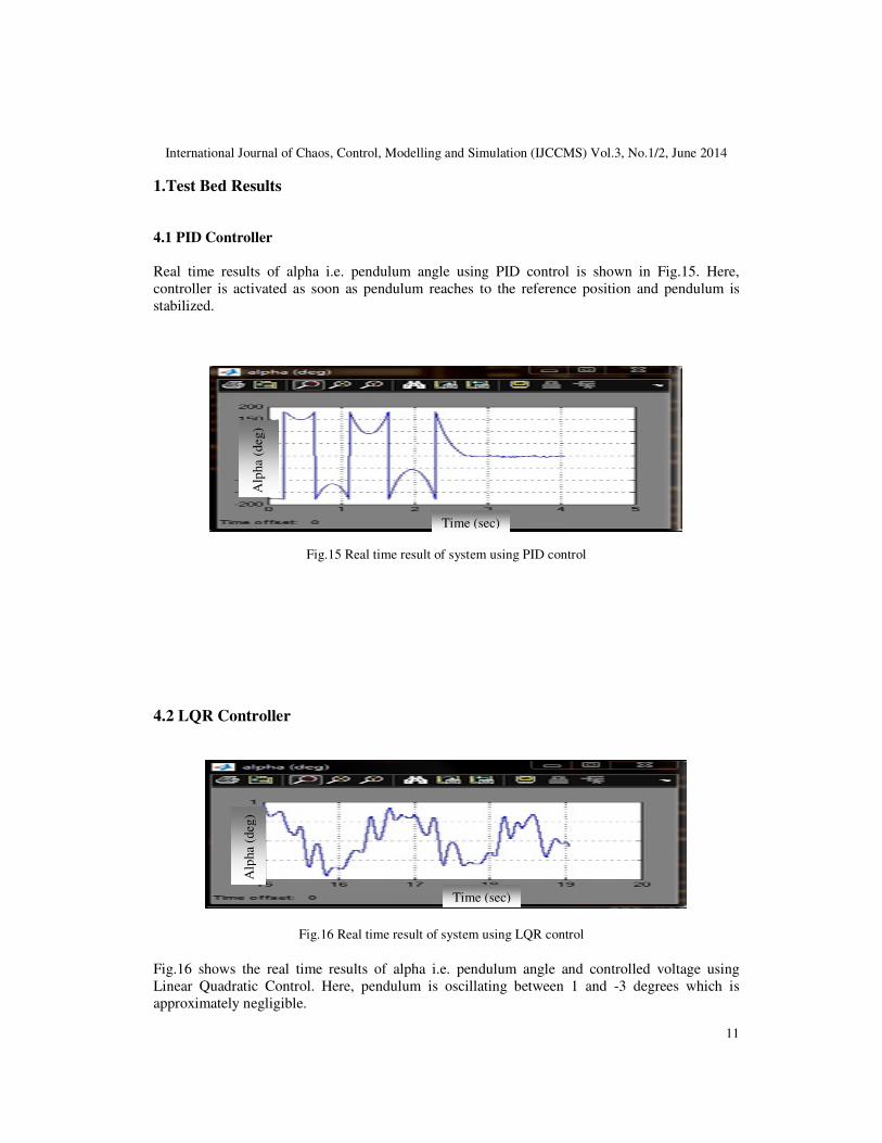
Real time results of alpha i.e. pendulum angle using PID control is shown in Fig.15. Here,

controller is activated as soon as pendulum reaches to the reference position and pendulum is

stabilized.

Fig.15 Real time result of system using PID control

4.2 LQR Controller

Fig.16 Real time result of system using LQR control

Fig.16 shows the real time results of alpha i.e. pendulum angle and controlled voltage using

Linear Quadratic Control. Here, pendulum is oscillating between 1 and -3 degrees which is

approximately negligible.

Time (sec)

Alp

ha

(deg

)

Time (sec)

Alp

ha

(deg

)


12

4.3 Fuzzy Logic Controller

Fig.17 Real time result of system using FUZZY LOGIC control

Fig.17 shows the real time results of alpha i.e. pendulum angle and controlled voltage using fuzzy

logic controller. Here, controller is activated as soon as pendulum reaches to the reference

position and pendulum is slightly oscillating.

1.Conclusion

5.1 COMPARISON OF SIMULATION RESULTS

In this section comparison of all the four controllers based on Simulation Results are discussed.

Parameters compared are percentage peak overshoot and rise time as shown in Table IV.

Table IV

Comparison of controllers based on simulation results

Controller Peak overshoot

(%Mp) Rise time (tr)

PID 0.3 0.1

LQR 4.8 0.1

Fuzzy Logic 0.09 0.05

H∞ 7.8 0.25

Comparing simulation results of all the four controllers, from the Table IV, it is concluded that,

percentage peak overshoot is less in case of Fuzzy Logic controller as compared to other three

controllers. Rise time is also less for this controller.

5.2 COMPARISON OF TEST BED RESULTS

Time (sec)

Alp

ha

(deg

)


13

In this section comparison of all the four controllers based on Test bed Results are discussed.

Parameters compared are percentage peak overshoot and rise time as shown in Table V.

Table V : Comparison of controllers based on Test Bed results

Controller Peak overshoot

(%Mp) Rise time (tr)

PID 2 0.3

LQR 2.5 0.5

Fuzzy Logic 10 0.1

H∞ -- --

Comparing test bed results of PID, LQR and FUZZY LOGIC, from the Table V it is concluded

that, percentage peak overshoot as well as rise time of response is less for LQR controller as

compared to PID and Fuzzy Logic controller

1.REFERENCES

[1] Quanser Inc.SRV02 Exp7 Inverted Pendulum.pdf.2003

[2] Quanser Inc.SRV02 Exp1 position control.pdf.2003

[3] T.Sugie and K. Fujimoto, “Controller design for an inverted pendulum based on approximate

linearization,” Int. J. of Robust and Nonlinear control, vol. 8, no 7, pp. 585-597, 1998.

[4] Katebi M R and M.H. Moradi (2001):“Predictive PID Controllers”. IEE Proc. Control Theory

Application, Vol. 148, No. 6; November 2001, pp. 478-487.

[5] K. Ang, G. Chong, and Y. Li, “PID control system analysis, design and technology,” IEEE

Trans.Control System Technology, vol. 13, pp. 559-576, July 2005.

[6] Md. Akhtaruzzaman and A. A. Shafie, “Modeling and Control of a Rotary Inverted Pendulum Using

Various Methods, Comparative Assessment and Result Analysis”, Proceedings of the 2010 IEEE,

International Conference on Mechatronics and Automation, August 4-7, 2010, Xi'an, China

[7] Chen Wei Ji, Fang Lei, Lei Kam Kin, I997 IEEE International Conference on Intelligent Processing

System October 28 - 31.“Fuzzy Logic Controller for an Inverted Pendulum System”

[8] Muskinja, N. and B. Tovornik, 2006. “Swinging up and stabilization of a real Inverted pendulum”.

IEEE Trans. Ind. Elect., 53. DOI: 10.1109/TIE.2006.870667

[9] Ximena CeliaM´endez Cubillos and Luiz Carlos Gadelha de Souza, 2009.“Using of H-Infinity Control

Method in Attitude Control System of Rigid-Flexible Satellite”, Hindawi Publishing Corporation

Mathematical Problems in Engineering Volume 2009, Article ID 173145, 9 pages

doi:10.1155/2009/173145

Documents

International Journal of Chaos, Control, Modelling and ...airccse.org/journal/ijccms/papers/3214ijccms01.pdfA Comparative study of controllers for stabilizing a Rotary Inverted Pendulum