Embed Size (px)
Citation preview

EDITORIAL OFFICE
EDITOR-IN-CHIEFMalcolm J. Crocker
MANAGING EDITORMarek Pawelczyk
ASSOCIATE EDITORSDariusz BismorNickolay IvanovZhuang Li
ASSISTANT EDITORSTeresa GlowkaJozef Wiora
EDITORIAL ASSISTANTKelcie Sharp
EDITORIAL BOARD
Jorge P. ArenasValdivia, Chile
Jonathan D. BlotterProvo, USA
Leonid GelmanCranfield, UK
Samir GergesFlorianopolis, Brazil
Victor T. GrinchenkoKiev, Ukraine
Colin H. HansenAdelaide, Australia
Hanno HellerBraunschweig, Germany
Hugh HuntCambridge, England
Finn JacobsenLyngby, Denmark
Dan MarghituAuburn, USA
Manohar Lal MunjalBangalore, India
David E. NewlandCambridge, England
Kazuhide OhtaFukuoka, Japan
Goran PavicVilleurbanne, France
Subhash SinhaAuburn, USA
International Journal ofAcoustics and Vibration
A quarterly publication of the International Institute of Acoustics and Vibration
Volume 18, Number 2, June 2013
EDITORIAL
The World of SoundMalcolm J. Crocker . . . . . . . . . . . . . . . . . . . . . . . . 50
ARTICLES
Forced Response Approach to Predict Parametric VibrationDishan Huang and Chenchen Fu . . . . . . . . . . . . . . . . . 51
Gear Fault Diagnosis Using Bispectrum Analysis of Active NoiseCancellation-Based Filtered Sound and Vibration Signals
Dibya Prakash Jena and S. N. Panigrahi . . . . . . . . . . . . 58
Recent Advances in Muffler AcousticsM. L. Munjal . . . . . . . . . . . . . . . . . . . . . . . . . . 71
A Dynamic Model of a Reinforced Thin Plate with Ribs of FiniteWidth
Jaclyn E. Sylvia and Andrew J. Hull . . . . . . . . . . . . . . 86
A Simplified Formula for Calculating the Sound Power Radiatedby Planar Structures
Yu Du and Jun Zhang . . . . . . . . . . . . . . . . . . . . . . 91
About the Authors . . . . . . . . . . . . . . . . . . . . . . . . . . 94
INFORMATION
Book Reviews . . . . . . . . . . . . . . . . . . . . . . . . . . . . . 96

Editor’s Space
The World of Sound
As human beings we are bathed
in a world of sound—the sounds of
nature—and man-made sound, some of it wanted and some
unwanted. We are dependent on sound and our acute sense
of hearing to communicate through speech and music. But
the sound on which we depend only exists in a small blan-
ket around our planet—the atmosphere. Noise can rob us of
the ability to communicate and can interfere with our sleep
and other activities. Noise also causes us stress, and in cases
where it is intense it can even damage our hearing. The engi-
neers among us try to ameliorate the effects of environmental
noise caused by road and rail traffic and aircraft. We mask the
noise of machinery though both passive and active means—
with mixed success.
But wait! There is a second world of sound—equally
important—but one we do not think about so much – the un-
derwater world of oceans, lakes, and rivers. This world teams
with life—fish, reptiles and mammals—porpoises and whales.
We can listen in to the strange sounds they make—their form
of communication. This second world of sound is also threat-
ened by man-made sounds from merchant and naval shipping.
Experts tell us that near shipping routes the underwater noise
is increasing by about three decibels every ten years. Mardi
Hastings gave us an excellent overview of sound in the under-
water world in “Sound in the Ocean: Acoustical Interactions
with Marine Animals,” her keynote lecture at ICSV18 in Rio
de Janeiro in July 2011.
What can we do as engineers to reduce underwater noise of
shipping? It is not easy. The predominant source is normally
the ship’s propeller. If that source is reduced then the power
plant noise can become dominant . Even with the best attempts
to vibration-isolate the power plant from the hull, the hull of a
ship will act as a “sounding board” and radiate noise into the
water, disturbing the marine life and announcing the presence
of the approaching ship to any of us “listening in.”
It is hard enough to reduce the noise of machinery in the at-
mosphere; but in water it is much harder. The fluid-loading
caused by water is much stronger than that of air. Modal
loading can normally be neglected in air, but not so in water,
where fluid-loading causes the complication of coupling be-
tween modes of vibration and increases the difficulty of mak-
ing accurate sound radiation predictions. Nicole Kessissoglou
is scheduled to review this topic in her keynote lecture “Nu-
merical Prediction of the Signature of Maritime Platforms” at
ICSV20 in Bangkok in July 2013.
I always find the keynote lectures of our ICSV congresses
informative. But I can honestly say that those by Mardi Hast-
ings and Nicole Kessissoglou have opened up a new world for
me.
Malcolm J. Crocker
Editor in Chief, International Journal of Acoustics
and Vibration (IIAV)
50 International Journal of Acoustics and Vibration, Vol. 18, No. 2, 2013
Forced Response Approach to Predict ParametricVibrationDishan Huang and Chenchen FuDept. of Mech. Eng, Shanghai University, Shanghai, P. R. China, 200072
(Received 16 August 2011; Revised 17 November 2012; Accepted 7 February 2013)
In this paper, forecast modelling based on modulation feedback is used to investigate the forced response of para-metric vibration with a damper. The system is excited by both the periodic coefficient and external force terms,which have different periods. In this study, the forced response is expressed as a linear combination of harmoniccomponents. By applying harmonic balance, the parametric equation is converted into a set of infinite-order linearalgebraic equations. Then, by taking the limit to infinity, all coefficients of the harmonic components in the forcedresponse are fully expanded into a series. The advantages of the presented approach are (1) the forced responseexpressed as a trigonometric series is easier to apply in practice and (2) all coefficients of the harmonic componentscan be determined by numerical computation. The accuracy of the proposed approach has been verified by com-paring resulting phase diagram trajectories with those obtained by the standard Runge-Kutta method. The resultsshow that the presented approach is suitable for the forced response approach and the nonlinear characterization ofparametric vibration.
1. INTRODUCTION
The problem with parametric vibration arises in manybranches of physics and engineering, and stability and re-sponse prediction are the two most significant dynamic prob-lems in the parametric vibration system. In the past, severalmethods have been used to study the stability of systems withperiodic coefficients. These include Hill’s method,1 the per-turbation method,2 the averaging approach, the Floquet the-ory with numerical integration,3 and Sinha’s numerical schemewith the shifted Chebyshev polynomial,4, 5 etc.
Many approaches, such as the general solution of the Math-ieu equation expressed in terms of auxiliary periodical func-tions,6 David’s transfer matrix method,7 linear combinationof the Floquet eigenvectors,8 and improved direct spectralmethod,9 etc., have been used to find the response expression.Some of these were able to efficiently find the forced responsein a multi-degree of freedom system in terms of periodic coef-ficients. However, the forced response would have more prac-tical value if it were expressed in the form of a Fourier series.For example, in the mechanical fault diagnosis for a rotor witha cross crack, such an expression would be irreplaceable.10 Sofar, none of the above mentioned approaches has directly con-sidered using a Fourier series solution.
This paper applies the concept of forecast modelling basedon modulation feedback to investigate the forced response.The investigation results in the mathematical derivation of theresponse in terms of a trigonometric series. Although the con-cept of forecast modelling has its roots in the modulation sys-tem, it can represent the physical characteristics of the para-metric vibration system.
2. MODULATION FEEDBACK CONCEPTION
Consider a system excited by both the periodic coefficientand external force terms, which have different periods, as de-scribed in Eq. (1):
d2x
dt2+ 2ζωn
dx
dt+ ω2
n(1 + β cosωot)x = F cosωpt. (1)
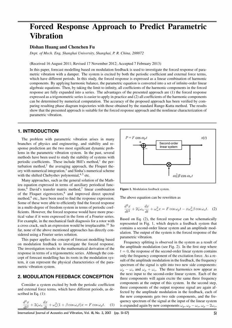
Figure 1. Modulation feedback system.
The above equation can be rewritten as
d2x
dt2+ 2ζωn
dx
dt+ ω2
nx = F cosωpt− xω2nβ cosωot. (2)
Based on Eq. (2), the forced response can be schematicallyrepresented in Fig. 1, which depicts a feedback system thatcontains a second-order linear system and an amplitude mod-ulation. The output of the system is the forced response of theparametric vibration.
Frequency splitting is observed in the system as a result ofthe amplitude modulation (see Fig. 2). In the first step wheret = 0, the response of the second-order linear system containsonly the frequency component of the excitation force. As a re-sult of the amplitude modulation in the feedback, the frequencyspectrum of the signal is split into two new side components:ωp − ωo and ωp + ωo. The three harmonics now appear asthe next input to the second-order linear system. Each of thethree components will again excite the same three frequencycomponents at the output of this system. In the second step,three components of the output response signal are again af-fected by the amplitude modulation in the feedback, each ofthe new components gets two side components, and the fre-quency spectrum of the signal at the input of the linear systemis expanded again by new components ωp, ωp−ωo, ωp− 2ωo,
International Journal of Acoustics and Vibration, Vol. 18, No. 2, 2013 (pp. 51–57) 51

D. Huang, et al.: FORCED RESPONSE APPROACH TO PREDICT PARAMETRIC VIBRATION
Figure 2. Frequency-splitting procedure (t ≥ 0, ∆t→ 0).
ωp+ωo, and ωp+2ωo. Figure 2 depicts the frequency-splittingprocess as it continues to infinity.
Assuming the process continues, the frequency splitting willeventually reach a state of balance unless the system is un-stable. Therefore, as a result of the frequency splitting, thereare many linear combinations of the harmonic components (ωpand ωo) in the system output, and they can be mathematicallyexpressed as follows:
x(t) =1
2
∞∑k=−∞
Akej(ωp+kωo)t+
1
2
∞∑k=−∞
Bke−j(ωp+kωo)t. (3)
Whether frequency splitting occurs in the given parametricvibration system also depends on the values ωo, ωp, andωp ± kωo, where, for frequency splitting to occur, the valuesmust be assumed to be close to ωn. When ωp ± kωo � ωn(k increases), the amplitude of the harmonic components willtend to zero because of decay, which is a characteristic of thesecond-order linear system. As a result, the energy of the har-monic components is concentrated on the narrow band rangearound the frequency ωp, where the coefficient Ak → 0 andBk → 0 when k →∞.
The key to the solution is to determine coefficients Ak andBk in Eq. (3).
3. SPLITTING EQUATION
Using Euler’s formula, Eq. (1) is changed to
d2x
dt2+ 2ζωn
dx
dt+ ω2
nx+ω2nβ
2(ejωot + e−jωot)x =
F
2(ejωpt + e−jωpt). (4)
Substituting Eq. (3) into Eq. (4) yields the following infiniteset of linear equations. The Ak and Bk terms can be found byapplying harmonic balance to both sides of Eq. (4):
ω2nβ
2A−1 +
[ω2n + 2jζωnωp − ω2
p
]A0 +
ω2nβ
2A1 = F ;
...
ω2nβ
2Ak−1 +
[ω2n + 2jζωn(ωp+kωo)− (ωp+kωo)
2]Ak +
ω2nβ
2Ak+1 = 0;
(k = . . . ,−m,−(m−1), . . . ,−3,−2,−1, 1, 2, 3, . . . ,m−1,m, . . .). (5)
ω2nβ
2B−1 +
[ω2n − 2jζωnωp − ω2
p
]B0 +
ω2nβ
2B1 = F ;
...
ω2nβ
2Bk−1 +
[ω2n − 2jζωn(ωp+kωo)− (ωp+kωo)
2]Bk +
ω2nβ
2Bk+1 = 0;
(k = . . . ,−m,−(m−1), . . . ,−3,−2,−1, 1, 2, 3, . . . ,m−1,m, . . .). (6)
The variable $k and its conjugate can be written as
$k = ω2n − (ωp+kωo)
2 + j2ζωn(ωp+kωo);
$∗k = ω2n − (ωp+kωo)
2 − j2ζωn(ωp+kωo);(k = . . . ,−m,−(m−1), . . . ,−3,−2,−1, 1, 2, 3, . . . ,
m−1,m, . . .); (7)
and
γ =ω2nβ
2. (8)
Combining 2m + 1 finite equations and applying all the coef-ficient relationships, a set of linear algebraic equations can beformed, here denoted as the splitting equation (Eq. (9)). Theequation is similar to Hill’s form. The matrices are noted as
WA = F1. (11)
For the same reason, another set of linear algebraic equationsis obtained for the coefficient B (Eq. (10)). It is denoted as
W∗B = F2; (12)
where ∗ indicates the conjugate, W is a complex symmetricmatrix, W∗ is the conjugate of W, and A and B are complexvectors.
4. CONJUGATE RELATIONa) Vector F
The coefficients Ak → 0 and Bk → 0 when k →∞. Thus,F1 = F2 = F, where F is a real vector and is expressed as
F = F∗ = [. . . , 0, 0, 0, F, 0, 0, 0, . . .]T . (13)
b) |A| = |B|Substitute Eq. (13) into Eqs. (11) and (12) and obtain
WA = W∗B. (14)
Applying a modulus operator to the above equation would re-sult in vectors A and B having the same modulus.
|A| = |B| or |Ak| = |Bk|. (15)
c) B = A∗
For the same modulus value in Eq. (3), which is the complexexponential series, the pair of indices (positive and negative)must result in a real function of time. Therefore, vectors Aand B must satisfy the following condition:
B = A∗. (16)
The vector B is a conjugate of vector A when k → ∞. Oncethe solution to vector A is found, the solution to vector B canbe obtained by using the conjugate relationship.
52 International Journal of Acoustics and Vibration, Vol. 18, No. 2, 2013
D. Huang, et al.: FORCED RESPONSE APPROACH TO PREDICT PARAMETRIC VIBRATION
$−m γγ $−m+1 γ
· · ·γ $−3 γ
γ $−2 γγ $−1 γ
γ $0 γγ $1 γ
γ $2 γγ $3 γ
· · ·γ $m−1 γ
γ $m
A−m
A−m+1
·A−3
A−2
A−1
A0
A1
A2
A3
·Am−1
Am
=
−γA−(m+1)
0·000F000·0
−γAm+1
. (9)
$∗−m γγ $∗
−m+1 γ· · ·
γ $∗−3 γγ $∗
−2 γγ $∗
−1 γγ $∗
0 γγ $∗
1 γγ $∗
2 γγ $∗
3 γ· · ·
γ $∗m−1 γγ $∗
m
B−m
B−m+1
·B−3
B−2
B−1
B0
B1
B2
B3
·Bm−1
Bm
=
−γB−(m+1)
0·000F000·0
−γBm+1
. (10)
5. DETERMINING COEFFICIENT Ak
The coefficient Ak is determined using the following alge-braic operations:(1) Consider the lower half of Eq. (9):
$0 γγ $1 γ
γ $2 γ· · ·
γ $m
A0
A1
A2
·Am
=
F − γA−1
00·
−γAm+1
. (17)
To solve Eq. (17), the set of frequency factors needs to be sub-stituted into the matrix, and these frequency factors are denotedas
α0 = $0;
α1 = $1 −γ2
α0;
...
αm = $m −γ2
α(m−1). (18)
Once the frequency factors are substituted into the coefficientmatrix, it can be simplified as an upper triangular matrix, andEq. (17) can be rewritten as
α0 γα1 γ
α2 γ· · ·
αm
A0
A1
A2
·Am
=
F − γA−1−γ(F−γA−1)
α0γ2(F−γA−1)
α0α1
·(−1)m γm(F−γA−1)∏m
i=1 αi−1− γAm+1
. (19)
Based on Eq. (19),
A0 = (F − γA−1)
(1
α0+
γ2
α20α1
+γ4
α20α
21α2
+
γ6
α20α
21α
22α3
+ . . .+(−1)mγm+1∏m+1
i=1 αi−1Am+1
). (20)
Given that Am → 0 while m→∞, A0 can be rewritten as
A0 = (F − γA−1)
(1
α0+
γ2
α20α1
+γ4
α20α
21α2
+
γ6
α20α
21α
22α3
+ . . .+γ2n−2
αn−1∏n−2i=0 α
2i
+ . . .
); (21)
A0 = (F − γA−1)S0; (22)
where
S0 =1
α0+
γ2
α20α1
+γ4
α20α
21α2
+
γ6
α20α
21α
22α3
+ . . .+γ2n−2
αn−1∏n−2i=0 α
2i
+ . . . (23)
For the same reason,
A1 = (F − γA−1)S1;
A2 = (F − γA−1)S2;
A3 = (F − γA−1)S3;
...Ak = (F − γA−1)Sk; (24)
where
S1 = − γ
α0α1− γ3
α0α21α2−
γ5
α0α21α
22α3− . . .− γ2n−1
α0(∏n−1i=1 α
2i )αn
− . . . ;
International Journal of Acoustics and Vibration, Vol. 18, No. 2, 2013 53
D. Huang, et al.: FORCED RESPONSE APPROACH TO PREDICT PARAMETRIC VIBRATION
S2 =γ2
α0α1α2+
γ4
α0α1α22α3
+
γ6
α0α1α22α
23α4
+ . . .+γ2n
α0α1(∏ni=2 α
2i )αn+1
+ . . . ;
S3 = − γ3
α0α1α2α3− γ5
α0α1α2α23α4−
γ7
α0α1α2α23α
24α5− . . .− γ2n+1
α0α1α2(∏n+1i=3 α
2i )αn+2
− . . . ;
...
Sk = (−1)k∞∑n=1
γ2n+k−2
(∏k−1j=0 αj)(
∏n+k−2i=k α2
i )αn+k−1. (25)
(2) Consider the upper half of Eq. (9):
$0 γγ $−1 γ
γ $−2 γ· · ·
γ $−m
A0
A−1A−2·
A−m
=
F − γA1
00·
−γA−m−1
.(26)
Equation (27) is obtained by applying the same logic and sub-stituting the frequency factors into Eq. (26):
α0 γ
α−1 γα−2 γ· · ·
α−m
A0
A−1A−2·
A−m
=
F − γA1
−γ(F−γA1)α0
γ2(F−γA1)α0α−1
·(−1)m γm(F−γA1)∏m
i=1 α−i+1− γA−m−1
. (27)
The frequency factors are
α0 = $0;
α−1 = $−1 −γ2
α0;
...
α−m = $−m −γ2
α−(m−1). (28)
The coefficients Am for Eq. (26) are
A0 = (F − γA1)R1;
A−1 = (F − γA1)R1;
A−2 = (F − γA1)R2;
A−3 = (F − γA1)R3;
...A−k = (F − γA1)Rk; (29)
where
R0 =1
α0+
γ2
α20α−1
+γ4
α20α
2−1α−2
+
γ6
α20α
2−1α
2−2α−3
+ . . .+γ2n−2
α−(n−1)∏n−2i=0 α
2−i
+ . . . ;
R1 = − γ
α0α−1− γ3
α0α2−1α−2
−
γ5
α0α2−1α
2−2α−3
− . . .− γ2n−1
α0(∏n−1i=1 α
2−i)α−n
− . . . ;
R2 =γ2
α0α−1α−2+
γ4
α0α−1α2−2α−3
+
γ6
α0α−1α2−2α
2−3α−4
+ . . .+
γ2n
α0α−1(∏ni=2 α
2−i)α−(n+1)
+ . . . ;
R3 = − γ3
α0α−1α−2α−3− γ5
α0α−1α−2α2−3α−4
−
γ7
α0α−1α−2α2−3α
2−4α−5
− . . .−
γ2n+1
α0α−1α−2(∏n+1i=3 α
2−i)α−(n+2)
− . . . ;
...
Rk = (−1)k∞∑n=1
γ2n+k−2
(∏k−1j=0 α−j)(
∏n+k−2i=k α2
−i)α−(n+k−1).
(30)
Based on A1 = (F − γA−1)S1 in Eq. (24) and A−1 = (F −γA1)R1 in Eq. (29), a set of linear algebraic equations can beset up. The solutions are
A−1 =FR1(1− γS1)
1− γ2R1S1;
A1 =FS1(1− γR1)
1− γ2R1S1. (31)
The final solution is achieved once Eq. (31) is substituted intoEq. (24) and Eq. (29):
A−k =1− γS1
1− γ2R1S1FRk; (k = 1, 2, 3, . . .);
Ak =1− γR1
1− γ2R1S1FSk; (k = 1, 2, 3, . . .). (32)
6. FORCED RESPONSE SOLUTION
Given the conjugate relationship of A and B, the forced re-sponse (Eq. (33)) can be expressed as a trigonometric series:
x(t) =1
2
∞∑k=−∞
Akej(ωp+kωo)t +
1
2
∞∑k=−∞
A∗ke−j(ωp+kωo)t.
(33)Let Ak = |Ak|ejφk , then A∗k = |Ak|e−jφk , and thus Eq. (33)can be rewritten as
x(t) =∞∑
k=−∞
|Ak| cos [(ωp + kωo)t+ φk] . (34)
54 International Journal of Acoustics and Vibration, Vol. 18, No. 2, 2013
D. Huang, et al.: FORCED RESPONSE APPROACH TO PREDICT PARAMETRIC VIBRATION
where φk = arg(Ak), and the coefficient Ak is determinedby Eq. (32). Therefore, the forced response of parametric vi-bration can be represented as a trigonometric series (Eq. (34)),and the coefficient Ak can be determined by Eq. (32).
7. RESONANCE CONDITION
The resonance condition of the parametric vibration can beroughly analysed using the given response solution (i.e., Ak).For greater accuracy, the computation of the coefficient valueAk should be carried out.
7.1. Main ResonanceBased on Eqs. (21) and (23), the frequency factor α0 is
the dominant contributor to the value of coefficient A0. Al-though all frequency factors (α1, α2,. . . ) affect the coefficientvalue A0, α0 has the greatest effect. Even when the damp-ing ratio ζ → 0, the main resonance response takes place inthe parametric vibration system when the force excitation fre-quency ωp is less than and close to the natural frequency ωn(ωp < ωn).
7.2. Combination Harmonic ResonanceBased on Eqs. (24) and (25), the frequency factor αk is the
dominant contributor to the value of Ak. Thus, |Ak| → ∞when αk = 0. That is,
αk = ω2n−(ωp+kωo)2+j2ζωn(ωp+kωo)−γ2/α(k−1) = 0.
(35)Therefore, the condition of combination harmonic resonancecan be approximately determined as follows:
ωp + kωo ≈ ωn. (36)
Since the term γ2/α(k−1) is a part of Eq. (35), the frequencypoint of a combination harmonic resonance occurs in the leftbias.
8. SPECTRAL PREDICTION
The following examples illustrate the transfer of responsefrom the time domain to the frequency domain using thetrigonometric series (Eq. (34)). The examples also testify thecondition of combination harmonic resonance.
Example 1: As an example of theoretical spectral predictionfor the forced response of parametric vibration, the followingconditions are given: natural frequency ωn = 25, force ex-citation frequency ωp = 10, frequency of period coefficientωo = 5, amplitude of excitation force F = 1, parametric mod-ulation index β = 0.3, and damping ratio ζ = 0.0001.
The forced response solution to Eq. (34) is determined asfollows:
x(t) = . . .+ |A−4| cos(−10t+ φ−4) +
|A−3| cos(−5t+ φ−3) + |A−2| cosφ−2 +|A−1| cos(5t+ φ−1) + |A0| cos(10t+ φ0) +
|A1| cos(15t+ φ1) + |A2| cos(20t+ φ2) +
|A3| cos(25t+ φ3) + |A4| cos(30t+ φ4) + . . . =
. . .+ |A−4| cos(10t− φ−4) +|A−3| cos(5t− φ−3) + |A−2| cosφ−2 +|A−1| cos(5t+ φ−1) + |A0| cos(10t+ φ0) +
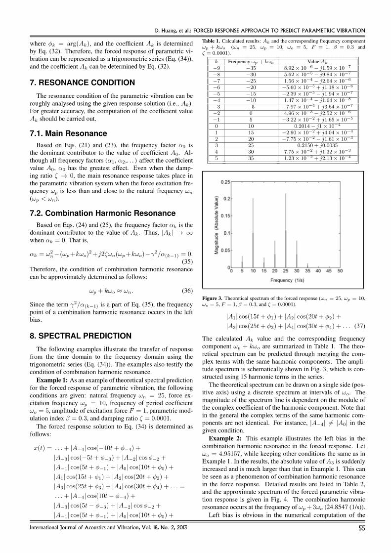
Table 1. Calculated results: Ak and the corresponding frequency componentωp + kωo (ωn = 25, ωp = 10, ωo = 5, F = 1, β = 0.3 andζ = 0.0001).
k Frequency ωp + kωo Value Ak
−9 −35 8.92× 10⁻⁶ − j1.59× 10−7
−8 −30 5.62× 10⁻⁵ − j9.84× 10−7
−7 −25 1.56× 10⁻⁴ − j2.64× 10−6
−6 −20 −5.60× 10⁻⁵ + j1.18× 10−6
−5 −15 −2.39× 10⁻⁵ − j1.94× 10−7
−4 −10 1.47× 10⁻⁴ − j1.64× 10−8
−3 −5 −7.97× 10⁻⁴ + j3.64× 10−7
−2 0 4.96× 10⁻³ − j2.52× 10−6
−1 5 −3.22× 10⁻² + j1.65× 10−5
0 10 0.2014− j1× 10−4
1 15 −2.90× 10⁻² + j4.04× 10−4
2 20 −7.75× 10⁻² − j1.61× 10−3
3 25 0.2150 + j0.00354 30 7.75× 10⁻² + j1.32× 10−3
5 35 1.23× 10⁻² + j2.13× 10−4
Figure 3. Theoretical spectrum of the forced response (ωn = 25, ωp = 10,ωo = 5, F = 1, β = 0.3, and ζ = 0.0001).
|A1| cos(15t+ φ1) + |A2| cos(20t+ φ2) +
|A3| cos(25t+ φ3) + |A4| cos(30t+ φ4) + . . . (37)
The calculated Ak value and the corresponding frequencycomponent ωp + kωo are summarized in Table 1. The theo-retical spectrum can be predicted through merging the com-plex terms with the same harmonic components. The ampli-tude spectrum is schematically shown in Fig. 3, which is con-structed using 15 harmonic terms in the series.
The theoretical spectrum can be drawn on a single side (pos-itive axis) using a discrete spectrum at intervals of ωo. Themagnitude of the spectrum line is dependent on the module ofthe complex coefficient of the harmonic component. Note thatin the general the complex terms of the same harmonic com-ponents are not identical. For instance, |A−4| 6= |A0| in thegiven condition.
Example 2: This example illustrates the left bias in thecombination harmonic resonance in the forced response. Letωo = 4.95157, while keeping other conditions the same as inExample 1. In the results, the absolute value of A3 is suddenlyincreased and is much larger than that in Example 1. This canbe seen as a phenomenon of combination harmonic resonancein the force response. Detailed results are listed in Table 2,and the approximate spectrum of the forced parametric vibra-tion response is given in Fig. 4. The combination harmonicresonance occurs at the frequency of ωp+3ωo (24.8547 (1/s)).
Left bias is obvious in the numerical computation of the
International Journal of Acoustics and Vibration, Vol. 18, No. 2, 2013 55

D. Huang, et al.: FORCED RESPONSE APPROACH TO PREDICT PARAMETRIC VIBRATION
Table 2. Calculated results: Ak and the corresponding frequency componentωp + kωo (ωn = 25, ωp = 10, ωo = 4.95157, F = 1, β = 0.3 andζ = 0.0001).
k Frequency ωp + kωo Value Ak
−9 ≈ −1.4ωn −7.47× 10⁻⁶ + j8.69× 10−6
−8 ≈ −1.2ωn −4.46× 10⁻⁵ + j5.19× 10−5
−7 ≈ −ωn −1.13× 10⁻⁴ + j1.31× 10−4
−6 ≈ −0.8ωn 6.48× 10⁻⁵ − j7.57× 10−5
−5 ≈ −0.6ωn −5.32× 10⁻⁵ + j6.29× 10−5
−4 ≈ −0.4ωn 1.55× 10⁻⁴ − j1.85× 10−4
−3 ≈ −0.2ωn −8.23× 10⁻⁴ + j9.82× 10−4
−2 ≈ 0 5.12× 10⁻³ − j6.12× 10−3
−1 ≈ 0.2ωn −3.33× 10⁻² + j3.98× 10−2
0 ≈ 0.4ωn 0.21− j0.251 ≈ 0.6ωn −0.07 + j1.352 ≈ 0.8ωn 0.07− j5.543 ≈ ωn −0.12 + j12.174 ≈ 1.2ωn −0.05 + j4.65 ≈ 1.4ωn −0.01 + j0.75
Figure 4. Theoretical spectrum of the forced response in the case of combi-nation harmonic resonance (ωn = 25, ωp = 10, ωo = 4.95157, F = 1,β = 0.3, and ζ = 0.0001).
combination harmonic resonance. This is due to the fact thatthe parametric modulation index β and the damping ratio ζ areboth factored into the parametric vibration equation.
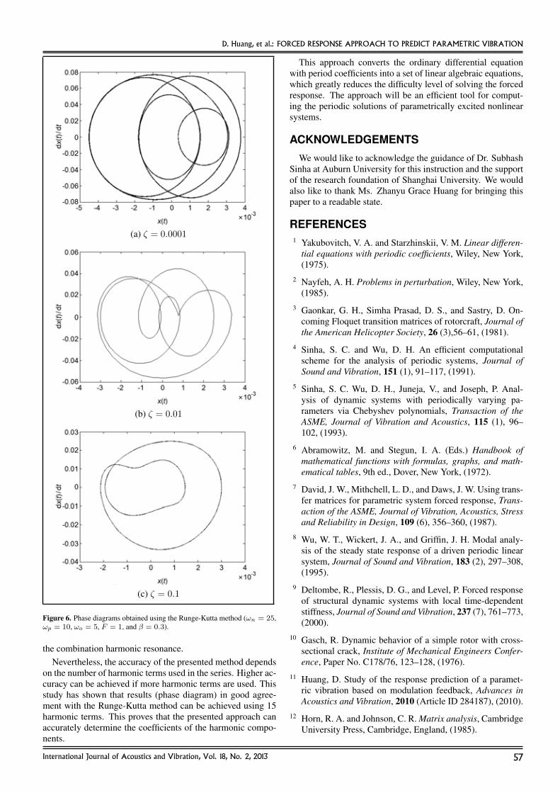
9. PHASE DIAGRAM
The phase diagram is sensitive to small changes in the forcedresponse. Based on Eq. (33), the detailed forced response isconstructed in the form of trigonometric series; thus, its phasediagram can be drawn in a phase plan, as shown in Fig. 5. Thefigure shows obvious quasiperiodic characteristics and sensi-tivity to the damping ratio.
For a complete investigation of the accuracy of the presentedapproach, the phase diagram was compared with one obtainedusing the fourth-order Runge-Kutta method (coding with Mat-lab function ode45), as shown in Fig. 6. All parameters arethe same as those in Example 1 except for the damping ratio.Thus, the phase diagram can be observed after the forced re-sponse approaches the steady state.
A comparison of the trajectories in Figs. 5 and 6 shows thatthe result of the presented approach is in good agreement withthe one obtained using the Runge-Kutta method. Therefore,the presented approach is valid in determining the coefficientsof harmonic components in a forced response and can be usedfor predicting the forced response solution.
(a) ζ = 0.0001
(b) ζ = 0.01
(c) ζ = 0.1
Figure 5. Phase diagrams obtained using the presented approach (ωn = 25,ωp = 10, ωo = 5, F = 1, and β = 0.3).
10. DISCUSSION AND CONCLUSIONS
The trigonometric series presented can completely deter-mine the forced response of a single-freedom parametric vi-bration with a damper. The complex coefficients work withvariables ωp, ωo, β, and ζ and has an advantage in both thetime and frequency domains when predicting the forced re-sponse. Once parameters are available, the approach can pre-dict the theoretical spectrum of the forced response and analyse
56 International Journal of Acoustics and Vibration, Vol. 18, No. 2, 2013
D. Huang, et al.: FORCED RESPONSE APPROACH TO PREDICT PARAMETRIC VIBRATION
(a) ζ = 0.0001
(b) ζ = 0.01
(c) ζ = 0.1
Figure 6. Phase diagrams obtained using the Runge-Kutta method (ωn = 25,ωp = 10, ωo = 5, F = 1, and β = 0.3).
the combination harmonic resonance.Nevertheless, the accuracy of the presented method depends
on the number of harmonic terms used in the series. Higher ac-curacy can be achieved if more harmonic terms are used. Thisstudy has shown that results (phase diagram) in good agree-ment with the Runge-Kutta method can be achieved using 15harmonic terms. This proves that the presented approach canaccurately determine the coefficients of the harmonic compo-nents.
This approach converts the ordinary differential equationwith period coefficients into a set of linear algebraic equations,which greatly reduces the difficulty level of solving the forcedresponse. The approach will be an efficient tool for comput-ing the periodic solutions of parametrically excited nonlinearsystems.
ACKNOWLEDGEMENTS
We would like to acknowledge the guidance of Dr. SubhashSinha at Auburn University for this instruction and the supportof the research foundation of Shanghai University. We wouldalso like to thank Ms. Zhanyu Grace Huang for bringing thispaper to a readable state.
REFERENCES1 Yakubovitch, V. A. and Starzhinskii, V. M. Linear differen-
tial equations with periodic coefficients, Wiley, New York,(1975).
2 Nayfeh, A. H. Problems in perturbation, Wiley, New York,(1985).
3 Gaonkar, G. H., Simha Prasad, D. S., and Sastry, D. On-coming Floquet transition matrices of rotorcraft, Journal ofthe American Helicopter Society, 26 (3),56–61, (1981).
4 Sinha, S. C. and Wu, D. H. An efficient computationalscheme for the analysis of periodic systems, Journal ofSound and Vibration, 151 (1), 91–117, (1991).
5 Sinha, S. C. Wu, D. H., Juneja, V., and Joseph, P. Anal-ysis of dynamic systems with periodically varying pa-rameters via Chebyshev polynomials, Transaction of theASME, Journal of Vibration and Acoustics, 115 (1), 96–102, (1993).
6 Abramowitz, M. and Stegun, I. A. (Eds.) Handbook ofmathematical functions with formulas, graphs, and math-ematical tables, 9th ed., Dover, New York, (1972).
7 David, J. W., Mithchell, L. D., and Daws, J. W. Using trans-fer matrices for parametric system forced response, Trans-action of the ASME, Journal of Vibration, Acoustics, Stressand Reliability in Design, 109 (6), 356–360, (1987).
8 Wu, W. T., Wickert, J. A., and Griffin, J. H. Modal analy-sis of the steady state response of a driven periodic linearsystem, Journal of Sound and Vibration, 183 (2), 297–308,(1995).
9 Deltombe, R., Plessis, D. G., and Level, P. Forced responseof structural dynamic systems with local time-dependentstiffness, Journal of Sound and Vibration, 237 (7), 761–773,(2000).
10 Gasch, R. Dynamic behavior of a simple rotor with cross-sectional crack, Institute of Mechanical Engineers Confer-ence, Paper No. C178/76, 123–128, (1976).
11 Huang, D. Study of the response prediction of a paramet-ric vibration based on modulation feedback, Advances inAcoustics and Vibration, 2010 (Article ID 284187), (2010).
12 Horn, R. A. and Johnson, C. R. Matrix analysis, CambridgeUniversity Press, Cambridge, England, (1985).
International Journal of Acoustics and Vibration, Vol. 18, No. 2, 2013 57

Gear Fault Diagnosis Using Bispectrum Analysisof Active Noise Cancellation-Based Filtered Soundand Vibration SignalsDibya Prakash Jena and S. N. PanigrahiSense and Process (SnP) Laboratory, School of Mechanical Sciences Indian Institute of Technology, Bhubaneswar- 751013, India
(Received 25 October 2011; Revised 8 January 2013; Accepted 6 February 2013)
Fault diagnosis using acoustical and vibration signal processing has received strong attention from many re-searchers over the last two decades. In the present work, the experiment has been carried out with a customizedgear mesh test setup in which the defects have been introduced in the driver gear. Classical statistical analysis in-cluding higher-order statistics, namely bispectrum analysis, has been incorporated to detect the defects. However,in order to improve the signal-to-noise ratio of the captured signals for accurate defect detection, an adaptive filter-ing has been proposed. Active noise cancellation (ANC) has been applied on the acoustical and vibration signalsas a denoising filter. The least mean square based ANC technique has been implemented considering the signalsfrom healthy gear meshing as the background noise. The focus of this experimental research is to evaluate theappropriateness of the ANC technique as a denoising tool and the subsequent bispectrum analysis for identifyingthe defects. The performance of the ANC filtering was evaluated with most widely accepted standard filters. Asynthetic signal, close in nature to the actual signal, has been investigated to ascertain the adequacy.
1. INTRODUCTION
Safety, reliability, efficiency, and performance of rotatingmachinery are major concerns in the industry. In this situa-tion, the task of condition monitoring and fault diagnosis ofrotating machinery has significant importance. Many meth-ods have already been widely used in a variety of industriesfor predictive maintenance. It has been widely accepted thatthe structural defects in rotating machinery components can bedetected through monitoring acoustical and/or vibration sig-nals. The machine condition monitoring process consists ofthree stages of signal processing: (1) acquisition of acoustic orvibration signals, (2) signal pre-processing and extraction ofthe fault feature, and (3) diagnosis of the defect.
Various signal processing techniques have been identifiedand proposed by many researchers in this context. The mostcommon method is the fast Fourier transform (FFT) to obtainthe power spectrum to investigate the frequency componentsof the entire signal. However, it is a well-known fact is that theacoustical or vibration signals from a rotating system is com-posed of a large number of non-stationary signals, particularlyin the presence of a localized, defect such as bearing pitting orgear tooth fracture. Short-time Fourier transform and relatedtime-frequency and time-scale techniques have often been usedto detect such non-stationary defect signatures. Another fact isthat typical defects in machinery components have been char-acterized by particular vibration patterns.1 Loutas et al. havereported that the acoustical emission (AE) technique is moreeffective in the early stages of defect identification comparedto vibration monitoring, particularly in the case of a crack inthe gear. Regionally linear behaviour of AE parameters hasbeen observed by them where the associated gradients change
proportionally with the crack propagation rate.2 Some poten-tial defects, namely spalling of the gears and bearings, clear-ances, etc., induce periodic impulses in acoustical and vibra-tion signals of rotating machines. Such impulses may excitethe eigenmodes of the structure and the sensor. The statisticalparameters such as the root mean square (RMS) value, kur-tosis, crest factor, skewness, peak value, and signal-to-noiseratio (SNR) are most widely used to detect the defect. Theseindicators are easy to implement; however, the complexity ofthe mechanisms involved may give rise to serious errors in in-terpretation. A detailed study was conducted by Dron et al.on the influence of certain parameters on the value of the crestfactor, kurtosis, and RMS value.3 In order to carry out con-dition monitoring of the gear meshing using acoustical andvibration signals analysis, the selection of such statistical in-dicators needs to be well suited to the impulsive nature of theexcitatory forces generated by the defects. Thus, reliability infault diagnosis can be achieved if, and only if, the acquired sig-nals are free from any background noise. Therefore, the majorchallenge is to remove background noise from acoustical andvibration signals captured at the faulty condition using appro-priate signal processing. The intention of signal denoising is tominimize the influence of the unwanted noise without affectingthe defect signatures.
Over the last decade, the performance of active noise can-cellation (ANC) systems has been improved primarily due tothe integration of digital signal processing. The merging of ac-tive noise cancellation techniques and digital signal processinghas enabled the control of noise dynamically and adaptively. Inpractice, active noise control is mainly used for duct-like sys-tems such as blowers, ventilation systems, or enclosures likeaircraft and vehicle cabins, headphones, and control rooms.
58 (pp. 58–70) International Journal of Acoustics and Vibration, Vol. 18, No. 2, 2013

D. P. Jena, et al.: GEAR FAULT DIAGNOSIS USING BISPECTRUM ANALYSIS OF ACTIVE NOISE CANCELLATION-BASED FILTERED SOUND. . .
The adaptive filtering deals with a least mean square (LMS)algorithm and an approach with reference signals with fixedlength of filter coefficients. The LMS algorithm is widely usedin adaptive filtering due to its computational simplicity and un-biased converging nature in a stationary environment.4 Adap-tive digital filters consist of two distinctive parts: (1) a digitalfilter to perform the desired signal processing and (2) an adap-tive algorithm using a reference signal and a residual error toadjust the coefficients (weights) of that filter. Based on a finiteimpulse response (FIR) structure, an adaptive digital filter witha filtered-x least mean square algorithm has been widely im-plemented in ANC applications due to its relative simplicity indesign and implementation.5 Gonzalez et al. have investigatedthe attenuation of engine noise using active noise cancellation.They have demonstrated that ANC can be considered a usefultool to reduce the sound pressure level of low-frequency noisesfor improving the acoustical comfort.6 On the other hand, theuse of higher-order spectral (HOS) analysis is an emerging areaof interest, particularly when the nonlinear system analysis isof interest.7–9 HOS analysis demonstrates the groups of fre-quencies and their interrelationships. This technique is alsocapable of explaining the origins of spectral peaks at certainvalues in the frequency spectrum. An HOS, especially bispec-trum analysis, has been used by many investigators for machin-ery condition monitoring.7 HOS has the potential to quantifynonlinearities using the time series signal. As a result, HOSmethods have been applied with partial success to rotating ma-chinery condition monitoring and fault diagnosis.8 In sum-mary, bispectrum analysis can identify the non-Gaussian pro-cesses.9 Collis, White, and Hammond have reported the basicprinciples of HOS and also have demonstrated the capabilityof HOS in yielding information which is unavailable throughinspection of second-order statistics such as the spectrum orcorrelation function.10
However, analysis using a bispectrum technique has beenused predominantly for condition monitoring purposes. Thebispectrum of a signal is the decomposition of the third mo-ment skewness of the signal over frequency, which supports theanalysis of systems with asymmetric nonlinearities. Similarly,another powerful technique known as trispectrum represents adecomposition of kurtosis over frequency. The bispectrum ofacoustical, vibration, or current signals has been extensivelyinvestigated by many researchers and reported suitable in faultdiagnosis of rotating system components, such as a damagedgear or bearing.9 Montero and Medina have demonstrated thetheoretical approach of implementing a bispectrum techniqueto identify a rolling bearing element defect.11 Li et al. havepresented fault detection and diagnosis of a gearbox in ma-rine propulsion systems using bispectrum analysis and artifi-cial neural networks. Incipient gear fault vibration signals of-ten have non-stationary features, are usually heavily corruptedby noise, and are often strongly coupled with the faults of othercomponents. Li et al. have demonstrated that the featuresof the gear fault vibration signals can be extracted effectivelyusing bispectrum analysis. Both the amplitude and phase in-formation can be preserved, and distinguished features can beextracted along the parallel lines of the bispectrum diagonal.12
Time-frequency analysis has been used by many investiga-
tors to analyse the non-stationarity of the signal.13 Sung, Tai,and Chen have employed wavelet transform to detect the lo-cation of tooth defects in a gear system precisely. They haveimplemented wavelet analysis on vibration signals for locat-ing gear defects and advantages of multi-resolution propertyof the wavelet.14 Jena, Panigrahi, and Kumar recently investi-gated adaptive wavelet transform for analysing non-stationaryvibration response from a faulty gear mesh system.15 Anotherimportant aspect of condition monitoring is establishing a re-liable online system to offer accurate fault diagnostic informa-tion for mechanical systems to prevent machinery performancedegradation, malfunction, or even catastrophic failures. More-over, machinery fault diagnosis information can also enablethe establishment of a maintenance program based on an earlywarning of incipient defects.
In the present work, an experiment has been carried out witha customized gear-meshing test setup in which defects havebeen introduced in the driver gear teeth. Two different defectconditions have been analysed: (1) a defect in one tooth and (2)a defect in two teeth. The acoustical and vibration signals arecaptured both in healthy conditions and with faulty gears. TheANC has been proposed for denoising purposea. An LMS-based adaptive filtering technique has been used on acousticaland vibration signals to improve the SNR of the signals in de-fect scenarios. The acoustical and vibration signals at healthyconditions have been used as reference signals for the adaptiveLMS filter. The statistical and bispectrum analysis have beenincorporated to evaluate the performance of the filtering tech-nique. A synthetic signal simulation analysis has been carriedout to understand the capability of the proposed method fol-lowed by experimental validations, which are explained andpresented in subsequent sections.
2. UNDERLYING THEORY
2.1. Hunting Tooth FrequencyIt is a well-known fact that gear-mesh frequency can be com-
puted by multiplying the number of teeth (T ) of a gear by thespeed of the gear (Gs). The number of teeth on the drive gearmultiplied by the speed of the drive gear must equal the num-ber of teeth on the driven gear multiplied by the speed of thedriven gear. The fractional gear-mesh frequencies generatedmay be caused by the common factor and the eccentric gear.Hunting tooth frequency (HTF) occurs when the same toothon each gear comes into mesh again.16 The HTF can be deter-mined by dividing the least common multiple of the teeth onthe two gears by the uncommon factor of the gear of interest.The product equals the number of revolutions the gear mustmake before the HTF occurs and can be expressed as
HTF = [1/(L/U)]× (1/Gs); (1)
where L is the least common multiple and U is the uncommonfactor of the gear. The HTF is not normally measurable be-cause it occurs infrequently; however, one can notice the samesituation occurring in the time domain signal. The broken toothon each gear generates a pulse each time when it goes intomesh. In the case of two broken teeth, consecutive pulses are
International Journal of Acoustics and Vibration, Vol. 18, No. 2, 2013 59

D. P. Jena, et al.: GEAR FAULT DIAGNOSIS USING BISPECTRUM ANALYSIS OF ACTIVE NOISE CANCELLATION-BASED FILTERED SOUND. . .
generated. The frequency of such impulse events observed ina time-domain signal is called HTF.16 Amplitude modulationof gear-mesh frequency and harmonics reveals useful informa-tion about the mesh (e.g., misaligned gears, improper backlash,loading, eccentricity, etc.). Gear-mesh frequency does not usu-ally reveal a broken, cracked, or chipped tooth except in rarecases when natural frequencies are not measurable. Gear-meshfrequency and amplitude can be modulated by the speed of theproblem gear. Some ghost frequencies may also be present dueto errors during gear manufacturing.17
2.2. Active Noise Cancellation Using an LMSAlgorithm
Acoustical and vibration signals acquired from the machinesfor diagnostic purposes may be either deterministic or ran-dom. Deterministic signals can be further classified as peri-odic and non-periodic, whereas random signals can be clas-sified as stationary and non-stationary.18 Useful informationcan be extracted from these signals by appropriate signal pro-cessing techniques. However, these acoustical and vibrationsignals often contain a lot of noise, which may also lead toincorrect conclusions. In such cases, techniques that enhancethe SNR are highly desired. Adaptive noise cancellation is onesuch technique that enhances SNR.17 An adaptive digital fil-ter consists of two stages of signal processing. The first stageis a digital filter, which processes the expected output signal,and second one is an algorithm to adjust weighting coefficientsof the digital filter. Two kinds of digital filters can be usedin ANC, namely infinite impulse response or FIR filters. Inthe present study, an FIR filter is used as the controller of thesystem.
Mathematically, if a linear FIR filter (discrete-time) has aseries of coefficients wl(n); (l = 0, 1 . . . , L − 1) and a seriesof continuous inputs {x(n) x(n− 1) . . . x(n−L+ 1)}, thenan expected output, d(n), occurs, and the output signal is usedto reduce noise from filter.19
Briefly, the procedures for the ANC system can be describedas follows:
1. Optimal selection of the order of filter coefficient L, stepsize µ, and the initial filter coefficients w0(n)
2. Evaluation of the output signal from the adaptive filter:
y(n) =L−1∑l=0
wl(n)x(n− 1) (2)
3. Measurement of the error signal as:
e(n) = d(n)− y(n) (3)
4. Updating of the adaptive filter coefficient using LMS al-gorithm
wl(n+ 1) = wl(n) + µx(n− l)e(n); (4)
where l = 0, 1, . . . , L− 1.
The step size and filter length are major parameters in adaptivefiltering. The step size value affects the convergence speed,steady-state error, and stability of the adaptive filter. A smallstep size ensures low steady-state error and decreased conver-gence speed. Large step size improves the convergence speedbut might cause instability.
The filter length affects the computational resource require-ments, convergence speed, and steady-state error. The optimalfilter length is decided by a trial-and-error process. However,simulation of adaptive filter is advised to be carried out to de-termine the most appropriate filter length. The filter lengthmust be greater than the number of significant taps in the im-pulse response of the unknown system.20 A long filter lengthcan reduce the steady-state error. Optimization of the filterlength that satisfies the application is highly desired.
2.3. Statistical ParametersTo obtain useful information from the time-domain acoustic
and vibration signals various statistical techniques have beendeveloped over the years. One of the parameters, namely, thecrest factor, which is defined as the ratio of maximum absolutevalue to the RMS value of the vibration signal, gives an ideaabout the occurrence of impulse in the time-domain signal. Inreal-time condition monitoring, an increased value of the crestfactor over a period of time indicates the presence of wear orpitting. Another powerful parameter called kurtosis measuresthe degree of peakiness of a distribution compared to a normaldistribution. In general, even statistical moments give infor-mation about spread. Mathematically, crest factor and kurtosisfor signal x(n) with N number of samples in the time domaincan be expressed as:
CrestFactor =CrestValueRMS value
=sup |x(n)|√
(1/N)∑N
n=1[x(n)]2(5)
and
Kurtosis =M4
M22
=(1/N)
∑Nn=1 (x(n)− x)
4[(1/N)
∑Nn=1 (x(n)− x)
2]2 ; (6)
where M4 and M2 are the fourth-order and second-order sta-tistical moment, respectively, and the x is the mean of the sig-nal.3, 21 The kurtosis and the crest factor parameters are verysensitive to the shape of the signal. The fourth-order momentof the signal gives a substantial weight to high amplitudes ofthe kurtosis. The crest factor attenuates the impact of an iso-lated event with high crest amplitude that only takes into ac-count the crest amplitude of this event. The kurtosis thereforeappears as a better indicator than the crest factor.21 But, inthe case of severe defects or a multiple defect scenario, thesestatistical parameters only provide the indication of the pres-ence of the defect but do not provide any information aboutthe severity of the defect. One of the limitations of the kurtosismethod is that the kurtosis value falls to 3 when the damage iswell advanced. This may be due to the higher relaxation timeof the impulsive response than the impulsive repetition period.Monitoring the overall RMS values can be more useful in suchcases. Another limitation is that the kurtosis method can give
60 International Journal of Acoustics and Vibration, Vol. 18, No. 2, 2013

D. P. Jena, et al.: GEAR FAULT DIAGNOSIS USING BISPECTRUM ANALYSIS OF ACTIVE NOISE CANCELLATION-BASED FILTERED SOUND. . .
variable and misleading results if measurements are taken onmachines in an unloaded condition.17
SNR is a measure used to compare the level of a desiredsignal to the level of the background noise. SNR can be definedas the inverse of coefficient of variation (Cv), (i.e., SNR =
1/Cv and Cv = σ/|µ|), where σ is the standard deviation andµ is the mean of a discrete signal. The absolute value is takenfor the mean to ensure Cv will be always positive.
The mean-square error (MSE) is widely used for filter-ing performance analysis. MSE measures the average of thesquares of the errors. The error is the difference between theobserved and estimated values. MSE is the second moment(about the origin) of the error and thus incorporates both thevariance of the estimator and its bias. For an unbiased estima-tor, the MSE is the variance.22 Mathematically, MSE can beexpressed as
MSE = (1/n)n−1∑i=0
(xi − yi)2; (7)
where n is the number of data points, xi is the i-th element ofx and yi is the i-th element of y.
2.4. Bispectrum EstimationHigher-order statistics is effective in studying feature extrac-
tion of the non-stationary signal. Higher-order statistics usu-ally refers to four major forms: (1) high-order moments, (2)high-order cumulants, (3) high-order moment spectrum, and(4) the high-order cumulant spectrum. The high-order cumu-lant of the random signal can be generated by the derivative ofthe second characteristic function. In practice, the higher-orderspectra of a signal must be estimated from a finite set of mea-surements. Essentially, there are two broad non-parametric ap-proaches: (1) the indirect method based on estimating the cu-mulant functions and then taking the Fourier transform and (2)the direct method based on a segment averaging approach.23
In the present analysis, indirect method is used to estimate thebispectrum.
Mathematically, for a random signal x(t), the second-orderspectral density (power spectrum) is given by
P (f) = E [X(f)X∗(f)]; (8)
where X(f) is the Fourier transform of x(t), E[. . .] indicatesthe expectation value (or equivalently the average over a statis-tical ensemble) and ∗ denotes the complex conjugate. Mathe-matically, the bispectrum can be expressed as
B(f1,f2) = E [X(f1)X(f2)X∗(f1 + f2)]. (9)
Due to the symmetries in the bispectrum, the region boundedby the lines f1 = 0 and f1 = f2 contains all the available in-formation. It is worth noting that if X(f1) = 0; X(f2) = 0; orX(f1 + f2) = 0, the bispectrum at f1, f2 is also zero, whichis not obvious. In short, signals resulting from the nonlin-ear interaction of some excitation components have a specificphase relationship with the excitations that caused them. Inthe power spectrum, the phase information is lost, and hence,this phase relationship between different frequencies cannot beexploited.12, 24
3. SIMULATED ANALYSIS
This section is intended to evaluate the performance of theproposed method of analysis using synthetic test signals. Asignal containing a number of sinusoidal bursts of progres-sively increasing frequency with respect to time was chosenfor the analysis in order to observe the frequency resolutiondependencies. The signal used can be mathematically writtenas
X[n] = x[n] +Gn; (10)
where
x[n] =m=10∑m=1
cos
[2πn
fmfs
(t− τm)
][u(t− τm)− u(t− δm)] ;
where fm = 15 mHz; τm = 0.0006 + 0.002(m − 1); δm =
τm + 0.0006; Gn ∼ N(0, 0.25); and fs = 50 kHz is the sam-pling frequency that is used to convert the continuous signalto a discrete one. The corresponding signals x[n] and X[n]
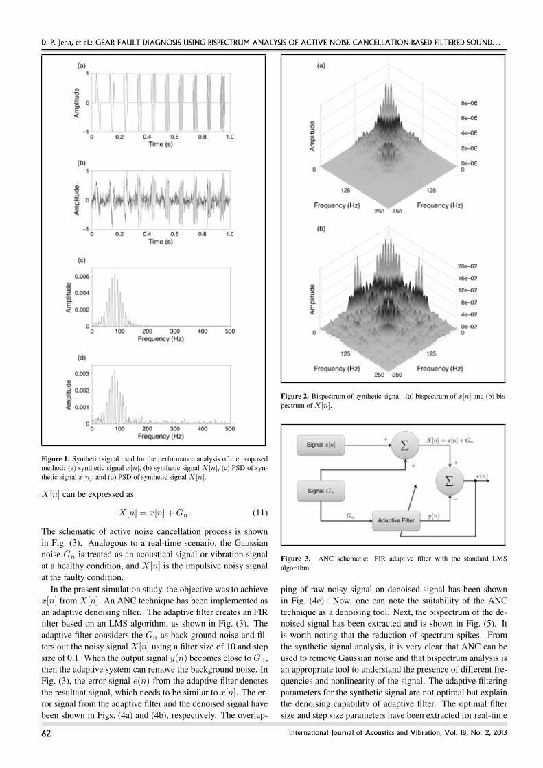
are shown in Figs. (1a) and (1b), respectively. To understandthe effect of Gaussian noise Gn on the synthetic signal x[n],the power spectrum density (PSD) has been extracted for bothx[n] and X[n], as shown in Figs. (1c) and (1d), respectively. Itis worth noting that from the PSD spectra, the impact of Gn isnot observed prominently.
Traditional correlation and power spectral analysis based onFourier transform could not extract useful information from thenonstable and nonlinear signals because the Fourier transformis based on the assumption that the signal is stationary. Thebispectrum has been proven to be effective in this situation. Itcan capture characteristic frequency, identify the phase infor-mation, and extract nonlinearity. To demonstrate the effect ofGn on synthetic signals, the bispectrum has been investigatedfor x[n] andX[n], as shown in Figs. (2a) and (2b), respectively.The bispectrum has been evaluated with 2048 numbers of fre-quency bins, 256 points of window length, and linear peak holdaveraging with 50% overlapping. A large window generates aPSD with small bias but results in a coarse PSD plot.
A small window generates a smooth PSD plot but leads tolarge bias. Overlap specifies the overlap in percentage, of themoving window that applies to the time series. This parameterdetermines how much data of the signal will be used for spacematrix. A large overlap reduces the variance of the resultingpower spectrum but increases computation time. The resultingbispectrum can detect the asymmetric nonlinearities in the in-put time series. From Figs. (2a) and (2b), one can note thatadditional spectrum spikes are visible after introducing Gn.The bispectrum of x[n] (see Fig. (2a)) explains the presenceof periodic impulses at different frequencies, which creates theprominent side band spikes. The bispectrum of X[n] has addi-tional spikes due to well-known quadratic phase coupling withGaussian noise Gn and synthetic signal x[n]. It is well knownthat the nonlinear couplings, including quadratic phase cou-pling, can be identified using bispectrum analysis.
In line with the proposed technique, adaptive noise cancel-lation was implemented to improve the SNR of the signal. Theperiodic burst signal x[n] is the desired signal, where Gaussiansignal Gn acts as the background noise. The resultant signal
International Journal of Acoustics and Vibration, Vol. 18, No. 2, 2013 61
D. P. Jena, et al.: GEAR FAULT DIAGNOSIS USING BISPECTRUM ANALYSIS OF ACTIVE NOISE CANCELLATION-BASED FILTERED SOUND. . .
Figure 1. Synthetic signal used for the performance analysis of the proposedmethod: (a) synthetic signal x[n], (b) synthetic signal X[n], (c) PSD of syn-thetic signal x[n], and (d) PSD of synthetic signal X[n].
X[n] can be expressed as
X[n] = x[n] +Gn. (11)
The schematic of active noise cancellation process is shownin Fig. (3). Analogous to a real-time scenario, the Gaussiannoise Gn is treated as an acoustical signal or vibration signalat a healthy condition, and X[n] is the impulsive noisy signalat the faulty condition.
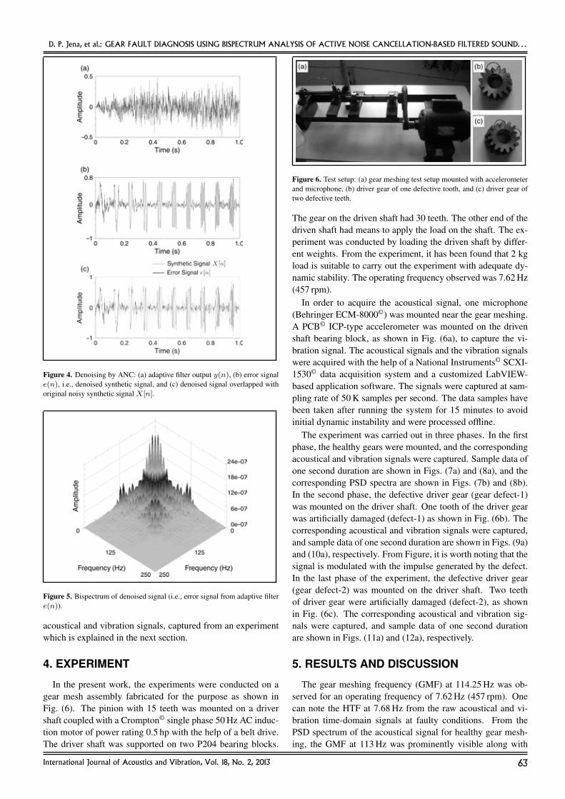
In the present simulation study, the objective was to achievex[n] from X[n]. An ANC technique has been implemented asan adaptive denoising filter. The adaptive filter creates an FIRfilter based on an LMS algorithm, as shown in Fig. (3). Theadaptive filter considers the Gn as back ground noise and fil-ters out the noisy signal X[n] using a filter size of 10 and stepsize of 0.1. When the output signal y(n) becomes close to Gn,then the adaptive system can remove the background noise. InFig. (3), the error signal e(n) from the adaptive filter denotesthe resultant signal, which needs to be similar to x[n]. The er-ror signal from the adaptive filter and the denoised signal havebeen shown in Figs. (4a) and (4b), respectively. The overlap-
Figure 2. Bispectrum of synthetic signal: (a) bispectrum of x[n] and (b) bis-pectrum of X[n].
Figure 3. ANC schematic: FIR adaptive filter with the standard LMSalgorithm.
ping of raw noisy signal on denoised signal has been shownin Fig. (4c). Now, one can note the suitability of the ANCtechnique as a denoising tool. Next, the bispectrum of the de-noised signal has been extracted and is shown in Fig. (5). Itis worth noting that the reduction of spectrum spikes. Fromthe synthetic signal analysis, it is very clear that ANC can beused to remove Gaussian noise and that bispectrum analysis isan appropriate tool to understand the presence of different fre-quencies and nonlinearity of the signal. The adaptive filteringparameters for the synthetic signal are not optimal but explainthe denoising capability of adaptive filter. The optimal filtersize and step size parameters have been extracted for real-time
62 International Journal of Acoustics and Vibration, Vol. 18, No. 2, 2013
D. P. Jena, et al.: GEAR FAULT DIAGNOSIS USING BISPECTRUM ANALYSIS OF ACTIVE NOISE CANCELLATION-BASED FILTERED SOUND. . .
Figure 4. Denoising by ANC: (a) adaptive filter output y(n), (b) error signale(n), i.e., denoised synthetic signal, and (c) denoised signal overlapped withoriginal noisy synthetic signal X[n].
Figure 5. Bispectrum of denoised signal (i.e., error signal from adaptive filtere(n)).
acoustical and vibration signals, captured from an experimentwhich is explained in the next section.
4. EXPERIMENT
In the present work, the experiments were conducted on agear mesh assembly fabricated for the purpose as shown inFig. (6). The pinion with 15 teeth was mounted on a drivershaft coupled with a Crompton© single phase 50 Hz AC induc-tion motor of power rating 0.5 hp with the help of a belt drive.The driver shaft was supported on two P204 bearing blocks.
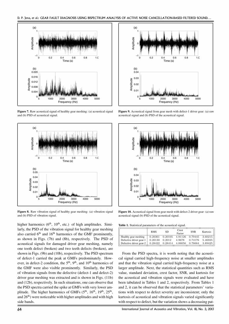
Figure 6. Test setup: (a) gear meshing test setup mounted with accelerometerand microphone, (b) driver gear of one defective tooth, and (c) driver gear oftwo defective teeth.
The gear on the driven shaft had 30 teeth. The other end of thedriven shaft had means to apply the load on the shaft. The ex-periment was conducted by loading the driven shaft by differ-ent weights. From the experiment, it has been found that 2 kgload is suitable to carry out the experiment with adequate dy-namic stability. The operating frequency observed was 7.62 Hz(457 rpm).
In order to acquire the acoustical signal, one microphone(Behringer ECM-8000©) was mounted near the gear meshing.A PCB© ICP-type accelerometer was mounted on the drivenshaft bearing block, as shown in Fig. (6a), to capture the vi-bration signal. The acoustical signals and the vibration signalswere acquired with the help of a National Instruments© SCXI-1530© data acquisition system and a customized LabVIEW-based application software. The signals were captured at sam-pling rate of 50 K samples per second. The data samples havebeen taken after running the system for 15 minutes to avoidinitial dynamic instability and were processed offline.
The experiment was carried out in three phases. In the firstphase, the healthy gears were mounted, and the correspondingacoustical and vibration signals were captured. Sample data ofone second duration are shown in Figs. (7a) and (8a), and thecorresponding PSD spectra are shown in Figs. (7b) and (8b).In the second phase, the defective driver gear (gear defect-1)was mounted on the driver shaft. One tooth of the driver gearwas artificially damaged (defect-1) as shown in Fig. (6b). Thecorresponding acoustical and vibration signals were captured,and sample data of one second duration are shown in Figs. (9a)and (10a), respectively. From Figure, it is worth noting that thesignal is modulated with the impulse generated by the defect.In the last phase of the experiment, the defective driver gear(gear defect-2) was mounted on the driver shaft. Two teethof driver gear were artificially damaged (defect-2), as shownin Fig. (6c). The corresponding acoustical and vibration sig-nals were captured, and sample data of one second durationare shown in Figs. (11a) and (12a), respectively.
5. RESULTS AND DISCUSSION
The gear meshing frequency (GMF) at 114.25 Hz was ob-served for an operating frequency of 7.62 Hz (457 rpm). Onecan note the HTF at 7.68 Hz from the raw acoustical and vi-bration time-domain signals at faulty conditions. From thePSD spectrum of the acoustical signal for healthy gear mesh-ing, the GMF at 113 Hz was prominently visible along with
International Journal of Acoustics and Vibration, Vol. 18, No. 2, 2013 63
D. P. Jena, et al.: GEAR FAULT DIAGNOSIS USING BISPECTRUM ANALYSIS OF ACTIVE NOISE CANCELLATION-BASED FILTERED SOUND. . .
Figure 7. Raw acoustical signal of healthy gear meshing: (a) acoustical signaland (b) PSD of acoustical signal.
Figure 8. Raw vibration signal of healthy gear meshing: (a) vibration signaland (b) PSD of vibration signal.
higher harmonics (6th, 10th, etc.) of high amplitudes. Simi-larly, the PSD of the vibration signal for healthy gear meshingalso carried 6th and 16th harmonics of the GMF prominently,as shown in Figs. (7b) and (8b), respectively. The PSD ofacoustical signals for damaged driver gear meshing, namelyone tooth defect (broken) and two teeth defects (broken), areshown in Figs. (9b) and (10b), respectively. The PSD spectrumof defect-1 carried the peak at GMFs predominately. How-ever, in defect-2 condition, the 5th, 9th, and 10th harmonics ofthe GMF were also visible prominently. Similarly, the PSDof vibration signals from the defective (defect-1 and defect-2)driver gear meshing was extracted and is shown in Figs. (11b)and (12b), respectively. In such situations, one can observe thatthe PSD spectra carried the spike at GMFs with very lower am-plitude. The higher harmonics of GMFs (5th, 16th, 19th, 25th,and 26th) were noticeable with higher amplitudes and with highside bands.
Figure 9. Acoustical signal from gear mesh with defect-1 driver gear: (a) rawacoustical signal and (b) PSD of the acoustical signal.
Figure 10. Acoustical signal from gear mesh with defect-2 driver gear: (a) rawacoustical signal (b) PSD of the acoustical signal.
Table 1. Statistical parameters of the acoustical signal.
RMS SD Crest SNR KurtosisFactorHealthy gear meshing 0.20361 0.20105 4.91126 0.79445 3.60215Defective driver gear-1 0.20130 0.2012 4.9678 0.74176 5.46935Defective driver gear-2 0.28422 0.28414 4.06056 0.76664 3.89425
From the PSD spectra, it is worth noting that the acousti-cal signal carried high-frequency noise at smaller amplitudesand that the vibration signal carried high-frequency noise at alarger amplitude. Next, the statistical quantities such as RMSvalue, standard deviation, crest factor, SNR, and kurtosis forthe acoustical and vibration signals were evaluated and havebeen tabulated in Tables 1 and 2, respectively. From Tables 1and 2, it can be observed that the statistical parameters’ varia-tions with respect to defect severity are inconsistent; only thekurtosis of acoustical and vibration signals varied significantlywith respect to defect, but the variation shows a decreasing pat-
64 International Journal of Acoustics and Vibration, Vol. 18, No. 2, 2013

D. P. Jena, et al.: GEAR FAULT DIAGNOSIS USING BISPECTRUM ANALYSIS OF ACTIVE NOISE CANCELLATION-BASED FILTERED SOUND. . .
Figure 11. Vibration response from gear mesh with defect-1 driver gear:(a) raw vibration signal and (b) PSD of the vibration signal.
Figure 12. Vibration response from gear mesh with defect-2 driver gear:(a) raw vibration signal and (b) PSD of the vibration signal.
Table 2. Statistical parameters of vibration signal.
RMS SD Crest SNR KurtosisFactorHealthy gear meshing 0.23287 0.23287 4.29431 0.76149 4.25658Defective driver gear-1 0.14548 0.08068 5.15058 1.59379 31.71135Defective driver gear-2 0.12390 0.12080 5.74989 0.67445 13.76904
tern with severe defect condition. This is possible due to thesharpness of the burst visible for defect-1 condition.17
For effective feature extraction of the nonstationary acous-tical and vibration signals, we implemented bispectrum analy-sis, which computes the single-sided bispectrum of a univari-ate time series using the FFT method. The bispectra were ex-tracted with 2048 frequency bins using 256 points of windowlength and linear peak hold, with parametersaveraging at 50%overlap. The resultant bispectrum had 24.42 Hz frequency res-olution.
The bispectrum for acoustical signals (healthy condition,
Figure 13. Bispectrum analysis of gear meshing acoustical signals: (a) healthygear meshing, (b) defective (one failure tooth) gear meshing, and (c) defective(two failure teeth) gear meshing.
defect-1, and defect-2) was extracted and are shown inFigs. (13a), (13b), and (13c), respectively. The bispectrum ofthe acoustical signal from healthy gear meshing had a majorspike at the GMF frequency (at ∼110 Hz). From Fig. (13),it can be noted that the bispectrum of faulty condition carriesa prominent peak at about 1500 Hz with wide side band. Insuch cases, it can also be observed that the high-frequency sig-nal components are introduced with a linear phase. So, thelow-frequency peaks for HTF and GMF are not discernible.Similarly, the bispectra for vibration signals (healthy condi-tion, defect-1, and defect-2) have been extracted and are shown
International Journal of Acoustics and Vibration, Vol. 18, No. 2, 2013 65

D. P. Jena, et al.: GEAR FAULT DIAGNOSIS USING BISPECTRUM ANALYSIS OF ACTIVE NOISE CANCELLATION-BASED FILTERED SOUND. . .
Figure 14. Bispectrum analysis of gear meshing vibration signals: (a) healthygear meshing, (b) defective (one failure tooth) gear meshing, and (c) defective(two failure teeth) gear meshing.
in Figs. (14a), (14b), and (14c), respectively. The bispectraof the vibration signals from healthy gear meshing shows ma-jor spikes at around 670 Hz, 1800 Hz, and 2100 Hz with wideside band. From Fig. (14), it can be noted that the bispectrumcarries major peaks at around 2100 Hz, 2500 Hz, and 2800 Hzwith wide side bands for faulty conditions. In such cases, an-other observation is that the high-frequency components areintroduced with the linear phase. The low-frequency peak ofHTF is visible for defect-1 condition but not prominently vis-ible for defect-2. It is worth noting from the bispectrum thatthe three major spikes are visible, which dominates other low-
frequency spikes in the faulty condition.From statistical analysis and bispectrum analysis, it is under-
stood that an adequate filtering is required to remove noise andmake signals more informative. Next, in line with the proposedsignal processing scheme, an ANC-based filtering techniquewas implemented. The filtering performance was comparedwith standard filters such as (a) FIR-based high-pass filter witha high cut-off frequency of 100 Hz with 51 taps; (b) FIR-basedlow-pass filter with a low cut-off frequency 5 kHz with 51 taps;(c) FIR-based band-pass filter with a high cut-off frequencyof 100 Hz and low cut-off frequency of 5 kHz with 51 taps;(d) rectangular half the width of the moving average filter; and(e) wavelet denoising using undecimated wavelet transform upto decomposition level 3, using db-2 as the mother waveletand soft thresholding at multiple levels using the SURE tech-nique.25
5.1. Acoustical Signal Analysis
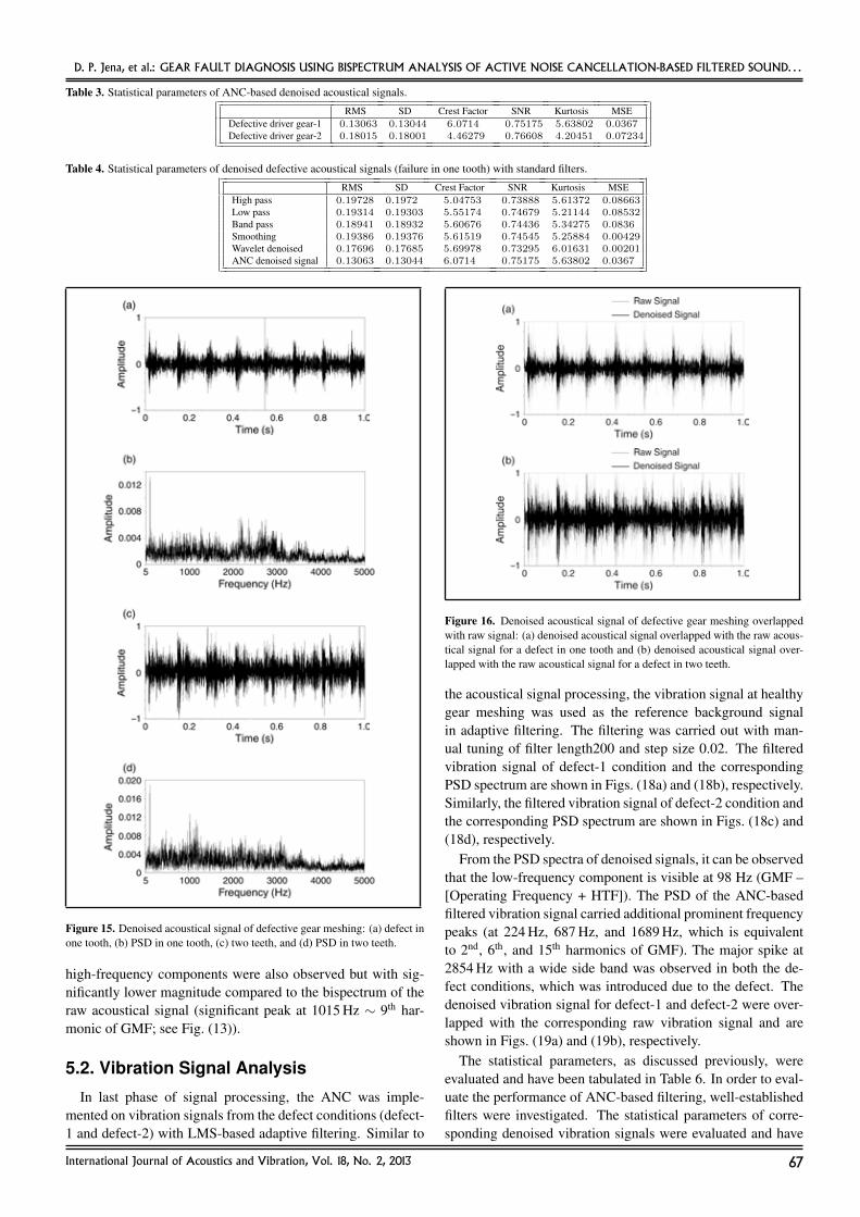
Active noise cancellation has been implemented with anLMS-based adaptive filtering for acoustical signals from thedefect conditions (defect-1 and defect-2). The acoustical signalfrom the healthy gear meshing was used as the reference back-ground signal in the adaptive filter. The filtering was carriedout with manual tuning of FIR filter length (200) and step size(0.093). The filtered acoustical signal of defect-1 and the cor-responding PSD spectrum are shown in Figs. (15a) and (15b),respectively. Similarly, the filtered signal of defect-2 conditionand the corresponding PSD spectrum are shown in Figs. (15c)and (15d), respectively.
From the PSD spectra of the denoised signals, it can benoted that the major low-frequency component is visible at99.9 Hz (GMF –[Operating Frequency + HTF]). The high-frequency components are also visible, but their magnitudeshave been reduced significantly. The denoised acoustical sig-nal for defect-1 and defect-2 were overlapped with the corre-sponding raw acoustical signal and are shown in Figs. (16a)and (16b), respectively.
The statistical parameters, as discussed previously, wereevaluated and have been tabulated in Table 3. In order to eval-uate the performance of ANC-based filtering, well-establishedfilters have been investigated. The statistical parameters of cor-responding denoised acoustical signals were evaluated and arepresented in Tables 4 and 5 for defect-1 and defect-2, respec-tively. It is worth noting from Tables 4 and 5 that the RMSand standard deviation decreased for the ANC-based denoisedsignal. However, the crest factor, SNR, and kurtosis values in-creased significantly compared to the raw acoustical signal anddenoised signals from other standard filters. The MSE param-eter was the lowest compared to other standard filters, whichexplains the retaining of the signal signature with minimal dis-tortion after ANC-based filtering.
Next, the bispectrum of denoised acoustical signals fordefect-1 and defect-2 conditions were extracted with the pa-rameters in Tables 4 and 5. The corresponding spectra areshown in Figs. (17a) and (17b), respectively. Based on bispec-trum analysis, it can be observed that the low-frequency com-ponent of HTF is clearly visible with high amplitudes. Other
66 International Journal of Acoustics and Vibration, Vol. 18, No. 2, 2013
D. P. Jena, et al.: GEAR FAULT DIAGNOSIS USING BISPECTRUM ANALYSIS OF ACTIVE NOISE CANCELLATION-BASED FILTERED SOUND. . .
Table 3. Statistical parameters of ANC-based denoised acoustical signals.
RMS SD Crest Factor SNR Kurtosis MSEDefective driver gear-1 0.13063 0.13044 6.0714 0.75175 5.63802 0.0367Defective driver gear-2 0.18015 0.18001 4.46279 0.76608 4.20451 0.07234
Table 4. Statistical parameters of denoised defective acoustical signals (failure in one tooth) with standard filters.
RMS SD Crest Factor SNR Kurtosis MSEHigh pass 0.19728 0.1972 5.04753 0.73888 5.61372 0.08663Low pass 0.19314 0.19303 5.55174 0.74679 5.21144 0.08532Band pass 0.18941 0.18932 5.60676 0.74436 5.34275 0.0836Smoothing 0.19386 0.19376 5.61519 0.74545 5.25884 0.00429Wavelet denoised 0.17696 0.17685 5.69978 0.73295 6.01631 0.00201ANC denoised signal 0.13063 0.13044 6.0714 0.75175 5.63802 0.0367
Figure 15. Denoised acoustical signal of defective gear meshing: (a) defect inone tooth, (b) PSD in one tooth, (c) two teeth, and (d) PSD in two teeth.
high-frequency components were also observed but with sig-nificantly lower magnitude compared to the bispectrum of theraw acoustical signal (significant peak at 1015 Hz ∼ 9th har-monic of GMF; see Fig. (13)).
5.2. Vibration Signal Analysis
In last phase of signal processing, the ANC was imple-mented on vibration signals from the defect conditions (defect-1 and defect-2) with LMS-based adaptive filtering. Similar to
Figure 16. Denoised acoustical signal of defective gear meshing overlappedwith raw signal: (a) denoised acoustical signal overlapped with the raw acous-tical signal for a defect in one tooth and (b) denoised acoustical signal over-lapped with the raw acoustical signal for a defect in two teeth.
the acoustical signal processing, the vibration signal at healthygear meshing was used as the reference background signalin adaptive filtering. The filtering was carried out with man-ual tuning of filter length200 and step size 0.02. The filteredvibration signal of defect-1 condition and the correspondingPSD spectrum are shown in Figs. (18a) and (18b), respectively.Similarly, the filtered vibration signal of defect-2 condition andthe corresponding PSD spectrum are shown in Figs. (18c) and(18d), respectively.
From the PSD spectra of denoised signals, it can be observedthat the low-frequency component is visible at 98 Hz (GMF –[Operating Frequency + HTF]). The PSD of the ANC-basedfiltered vibration signal carried additional prominent frequencypeaks (at 224 Hz, 687 Hz, and 1689 Hz, which is equivalentto 2nd, 6th, and 15th harmonics of GMF). The major spike at2854 Hz with a wide side band was observed in both the de-fect conditions, which was introduced due to the defect. Thedenoised vibration signal for defect-1 and defect-2 were over-lapped with the corresponding raw vibration signal and areshown in Figs. (19a) and (19b), respectively.
The statistical parameters, as discussed previously, wereevaluated and have been tabulated in Table 6. In order to eval-uate the performance of ANC-based filtering, well-establishedfilters were investigated. The statistical parameters of corre-sponding denoised vibration signals were evaluated and have
International Journal of Acoustics and Vibration, Vol. 18, No. 2, 2013 67

D. P. Jena, et al.: GEAR FAULT DIAGNOSIS USING BISPECTRUM ANALYSIS OF ACTIVE NOISE CANCELLATION-BASED FILTERED SOUND. . .
Table 5. Statistical parameters of denoised defective acoustical signals (failure in two teeth) with standard filters.
RMS SD Crest Factor SNR Kurtosis MSEHigh Pass (100 Hz) 0.27711 0.27705 3.58247 0.7645 3.96218 0.18548Low Pass (5000 Hz) 0.27191 0.27183 4.17771 0.77238 3.78861 0.18355Band Pass (100–5000 Hz) 0.26517 0.2651 4.22489 0.77082 3.84271 0.1785Smoothing (rectangular) 0.27458 0.27451 4.22522 0.77017 3.79728 0.00785Wavelet denoised (UWT) 0.25239 0.25231 4.28111 0.76607 3.9837 0.00408ANC denoised signal 0.18015 0.18001 4.46279 0.76608 4.20451 0.07234
Table 6. Statistical parameters of the ANC-based denoised vibration signal.
RMS SD Crest Factor SNR Kurtosis MSEDefective driver gear-1 0.14762 0.06516 7.37072 2.09151 20.75317 0.00453Defective driver gear-2 0.09081 0.08566 8.59815 0.74164 11.54897 0.00869
Figure 17. Bispectrum of denoised acoustical signals by ANC: (a) bispectrumspectrum of the denoised acoustical signal at defect in one tooth and (b) bis-pectrum spectrum of the denoised acoustical signal at defect in two teeth.
been presented in Tables 7 and 8 for defect-1 and defect-2, re-spectively. Similar to the statistics of the denoised acousticalsignal, it is worth noting from Tables 7 and 8 that the RMS andstandard deviation are decreased for the ANC-based denoisedsignal. However, the crest factor, SNR, and kurtosis values in-creased significantly compared to the raw vibration signal anddenoised signals from other standard filters. The MSE param-eter is was the lowest compared to other standard filters, whichexplains the retaining of signal signature with minimal distor-tion after ANC-based filtering.
Finally, the bispectrum of denoised vibration signals fordefect-1 and defect-2 conditions was extracted, similar to theacoustical signal processing. The corresponding spectra areshown in Figs. (20a) and (20b), respectively. From the bis-
Figure 18. Denoised vibration signal of defective gear meshing: (a) one tooth,(b) PSD in one tooth, (c) two teeth, and (d) PSD in two teeth.
pectrum, it can be observed that the low-frequency componentof HTF is clearly visible with high amplitudes. Other high-frequency components were also observed but with signifi-cantly lower magnitude compared to the bispectrum of the rawacoustical signal (significant peak at ∼2854 Hz, see Fig. (14)).With an increase in defect severity, other high-frequency com-ponents are introduced which dominate the HTF spike magni-tude. The proposed method was tested with 20 test samples,and the observed results are repeatable. in summary, the pro-
68 International Journal of Acoustics and Vibration, Vol. 18, No. 2, 2013

D. P. Jena, et al.: GEAR FAULT DIAGNOSIS USING BISPECTRUM ANALYSIS OF ACTIVE NOISE CANCELLATION-BASED FILTERED SOUND. . .
Table 7. Statistical parameters of the denoised defective vibration signal (failure in one tooth) with standard filters.
RMS SD Crest Factor SNR Kurtosis MSEHigh pass (100 Hz) 0.13635 0.07964 7.1434 1.48993 32.72079 0.01597Low pass (5000 Hz) 0.14491 0.07976 7.38803 1.60825 30.62829 0.01584Band pass (100–5000 Hz) 0.13611 0.07886 7.46802 1.50524 31.67959 0.01578Smoothing (rectangular) 0.14399 0.07796 7.43385 1.64244 30.6741 0.00064Wavelet denoised (UWT) 0.1436 0.07723 7.41479 1.65786 34.98493 0.00005ANC denoised signal 0.14762 0.06516 7.37072 2.09151 20.75317 0.00453
Table 8. Statistical parameters of the denoised defective acoustical signal (failure in two teeth) with standard filters.
RMS SD Crest Factor SNR Kurtosis MSEHigh pass (100 Hz) 0.12066 0.11801 8.19805 0.66358 14.50472 0.02853Low pass (5000 Hz) 0.12315 0.12004 8.23485 0.67596 13.41093 0.0291Band pass (100–5000 Hz) 0.12019 0.11752 8.27487 0.66537 14.13218 0.02837Smoothing (rectangular) 0.12107 0.1179 8.28729 0.67947 13.30746 0.00103Wavelet denoised (UWT) 0.11854 0.1153 8.32403 0.66858 14.78804 0.00014ANC denoised signal 0.09081 0.08566 8.59815 0.74164 11.54897 0.00869
Figure 19. Denoised vibration signal of defective gear meshing overlappedwith raw signal: (a) one tooth and (b) two teeth.
posed method can be deemed suitable and reliable in gear teethfault diagnosis using emitted acoustical signals or induced vi-bration response.
6. CONCLUSIONS
Statistical parameters provide information about the pres-ence of the defects. However, they cannot explain the severityof the defect. The HTF is not observed from the PSD spec-tra of the acoustical and vibration signals from faulty condi-tions. The experimental analysis reveals that the ANC is anappropriate denoising tool for these faulty conditions. Acous-tical and vibration signals from the healthy gear meshing sce-nario can be used as the background noise for the LMS-basedadaptive filter. The performance of the proposed denoisingtechnique is superior to most of the well-established standardfilters. The improvement in SNR, crest factor, and kurtosisare significantly noteworthy after the denoising of acousticaland vibration signals from the faulty condition (defect-1 anddefect-2) as compared to the raw signal. The bispectrum of de-noised acoustical and vibration signal carries prominent spikesat lower frequencies, which explains the presence of HTF inthe faulty condition. From identification of HTF, one can en-sure the presence of faulty teeth in gear meshing. In summary,
Figure 20. Bispectrum of denoised vibration signals by ANC: (a) bispectrumspectrum in one tooth and (b) bispectrum spectrum in two teeth.
the bispectrum of denoised (ANC-based) acoustical and vibra-tion signals provides a clearer view about the presence of faultin gear teeth.
ACKNOWLEDGEMENTS
The authors want to acknowledge support from Dr. RajeshKumar, Mechanical Engineering Department, SLIET Lon-gowal for execution of the experiment. The first author ac-knowledges generous funding received from the Ministry ofHuman Resource Development, Government of India that al-lowed this work to be carried out.
International Journal of Acoustics and Vibration, Vol. 18, No. 2, 2013 69

D. P. Jena, et al.: GEAR FAULT DIAGNOSIS USING BISPECTRUM ANALYSIS OF ACTIVE NOISE CANCELLATION-BASED FILTERED SOUND. . .
Bibliography1 Parker Jr., B. E., Ware, H.A., Wipf, D. P., Tompkins, W. R.,
Clark, B. R., Larson, E. C., and Poor, H. V. Fault diagnos-tics using statistical change detection in the bispectral do-main, Mech. Syst. Signal Process.,14(4), 561–570, (2000).
2 Loutas, T. H., Sotiriades, G., Kalaitzoglou, I. andKostopoulos, V. Condition monitoring of a single-stagegearbox with artificially induced gear cracks utilizing on-line vibration and acoustic emission measurements, Appl.Acoust., 70(9), 1148–1159, (2009).
3 Dron, J. P., Rasolofondraibe, L., Chiementin, X., and Bo-laers, F. A comparative experimental study on the use ofthree denoising methods for bearing defect detection, Mec-canica, 45 (2), 265–277, (2010).
4 Troparevskya, M. I. and D’Attellis, C. E. On the conver-gence of the LMS algorithm in adaptive filtering, SignalProcess., 84 (10), 1985–1988, (2004).
5 Liao, C. W. and Lin, J. Y. New FIR filter-based adaptive al-gorithms incorporating with commutation error to improveactive noise control performance, Automatica, 43 (2), 325–331, (2007).
6 Gonzalez, A., Ferrer, M., Diego, M. D., Piñero, G., andGarcia-Bonito, J.J. Sound quality of low-frequency and carengine noises after active noise control, J. Sound Vib., 265(3), 663–679, (2003).
7 Wang, W. J., Wu, Z. T., and Chen, J. Fault identificationin rotating machinery using the correlation dimension andbispectra, Nonlinear Dyn., 25 (4), 383–393, (2001).
8 Jiang, L., Liu, Y., Li, X., and Tang, S. Using bispectral dis-tribution as a feature for rotating machinery fault diagnosis,Measurement, 44 (7), 1284–1292, (2011).
9 Boltezar, M. and Slavic, J. Fault detection of DC elec-tric motors using the bispectral analysis, Meccanica 41 (3),283–297, (2006).
10 Collis, W. B., White, P. R., and Hammond, J. K. Higher-order spectra: The bispectrum and trispectrum, Mech. Syst.Signal Process., 12 (3), 375–394, (1998).
11 Montero, F. E. H. and Medina, O. C. The application of bis-pectrum on diagnosis of rolling element bearings: A theo-retical approach, Mech. Syst. Signal Process., 22 (3), 588–596, (2008).
12 Li, Z., Yan, X., Yuan, C., Zhao, J., and Peng, Z. Fault de-tection and diagnosis of a gearbox in marine propulsionsystems using bispectrum analysis and artificial neural net-works, J. Marine Sci. Appl., 10, 17–24, (2011).
13 Jena, D. P. and Panigrahi, S. N. Bearing and gear fault diag-nosis using adaptive wavelet transform of vibration signals,Procedia Eng., 50, 265–274, (2012).
14 Sung, C. K., Tai, H. M., and Chen, C. W. Locating defectsof a gear system by the technique of wavelet transform,Mech. Mach. Theory, 35 (8), 1169–1182, (2000).
15 Jena, D. P., Panigrahi, S. N., and Kumar, R. Gear faultidentification and localization using analytic wavelet trans-form of vibration signal, Measurement, 46 (3), 1115–1124,(2013).
16 Taylor, J. I. The vibration analysis handbook, 2nd ed., VCI,(2003).
17 G. and Robert X., Condition monitoring and control for in-telligent manufacturing, 1st ed., Springer, (2006).
18 Learned, R. E. and Willsky, A. S. A wavelet packet ap-proach to transient signal classification, Center for Intel-ligent Control Systems, 380, (1993).
19 Chen, S. R. and Too, G. P. J. Simulations and experimentsfor hybrid noise control systems, Appl. Acoust., 70 (2),247–255, (2009).
20 Loy, N. J. An engineer’s guide to FIR digital filters, PrenticeHall (1987).
21 Dron, J. P., Bolaers, F., and Rasolofondraibe, I. Improve-ment of the sensitivity of the scalar indicators (crest factor,kurtosis) using a de-noising method by spectral subtraction:application to the detection of defects in ball bearings, J.Sound Vib., 270 (1–2), 61–73, (2004).
22 DeGroot, M. H. and Schervish, M. J. Probability and statis-tics, 2nd ed., Addison-Wesley, (1980).
23 Choudhury, M. A. A. S., Shah, S. L., and Thornhill, N.F. Diagnosis of process nonlinearities and valve stiction:Data driven approaches, 1st ed., Springer, (2008).
24 Courtney, C. R. P., Neild, S. A., Wilcox, P. D., andDrinkwater, B. W. Application of the bispectrum for detec-tion of small nonlinearities excited sinusoidally, J. SoundVib., 329 (20), 4279–4293, (2010).
25 Shin, K. and Hammond, J. Fundamentals of signal pro-cessing for sound and vibration engineers, 1st ed., Wiley,(2008).
70 International Journal of Acoustics and Vibration, Vol. 18, No. 2, 2013

Recent Advances in Muffler AcousticsM. L. MunjalFacility for Research in Technical Acoustics (FRITA), Department of Mechanical Engineering, Indian Institute ofScience, Bangalore — 560 012, India.
(Received 23 December 2011; Accepted 14 November 2012)
Exhaust noise in engines has always been a major source of automotive noise. Challenges for muffler design havebeen constraints on size, back pressure, and, of course, the cost. Designing for sufficient insertion loss at theengine firing frequency and the first few harmonics has been the biggest challenge. Most advances in the designof efficient mufflers have resulted from linear plane wave theory, making use of the transfer matrix method. Thisreview paper deals with evaluating approximate source characteristics required for prediction of the unmuffledintake and exhaust noise, making use of the electroacoustical analogies. In the last few years, significant advanceshave been made in the analysis of variable area perforated ducts, transverse plane wave analysis of short elliptical aswell as circular chambers, double-tuned expansion chambers and concentric tube resonators, catalytic converters,diesel particulate filters, air cleaners, etc. The development of long strand fibrous materials that can be used inhot exhaust systems without binders has led to the use of combination mufflers in exhaust systems. Breakthroughshave been achieved in the prediction and control of breakout noise from the elliptical and circular muffler shell aswell as the end plates of typical mufflers. Diesel particulate filters and inlet air cleaners have also been modeledacoustically. Some of these recent advances are the subject of this review paper.
1. INTRODUCTION
Mufflers are essentially low-pass acoustical filters. Makinguse of electroacoustical analogies,1 lumped inductance and ca-pacitance of electrical wave filter are represented in mufflersby connecting pipes (or ducts) and chambers (or plenums),respectively. Helmholtz resonators of musical acoustics havealso found their counterpart here in the form of a hole-cavityresonator. Although the science of acoustics of ducts and muf-flers is over 150 years old,2 the first comprehensive experimen-tal investigation on analysis and design of mufflers for internalcombustion engines was reported by Davis et al. in 1954.3
The classical 1-D or plane wave theory with progressive wavesmoving in either direction led to the development of the trans-fer matrix method (TMM), which is ideally suited for acousti-cal modelling of cascaded elements constituting typical auto-motive mufflers.4
The TMM makes use of the standing wave variables to movefrom one element to the next in the cascade. Computationally,successive multiplication of transfer matrices is much faster aswell as more convenient than formulation and simultaneous so-lution of a large number of linear algebraic equations. In fact,a heuristic study of the transfer matrix multiplication processled to the development of a user-friendly algebraic algorithm,5
which in turn helped in a rational synthesis of 1-D acousticalfilters6 as well as vibration isolators.7
Morfey’s work on the sound generation and propagation inducts with mean flow8 indicated that the convective effect ofmean flow9 is to augment the flow-acoustical power of the for-ward wave and reduce that of the rearward (or reflected) wave.This led to the definition of convective (or flow acoustical) statevariables (pc, vc) that are linearly related in the classical (sta-tionary medium) state variables (p, v). Replacement of (p, v)with (pc, vc) yields identically similar expressions for inser-tion loss (IL) of a muffler with incompressible mean flow.10
The transformation relations between (p, v) and (pc, vc) enableconversion of the transfer matrices in classical state variableswith a moving medium to their counterparts in convective statevariables and vice versa.
A Helmholtz resonator introduces a sharp peak at its reso-nance frequency.10 However, designing an automotive mufflerrequires wide-band domes. Therefore, a designer would usepipes with extended perforations opening into an annular cav-ity. The resulting concentric tube resonator was first modelledby Sullivan and Crocker,11 making use of a 1-D control vol-ume approach. The resulting coupled equations were solved bywriting the acoustical field in the annular cylindrical cavity asa summation of natural modes satisfying the rigid-wall bound-ary conditions at the two ends. Sullivan followed it up witha segmentation approach which was applicable to a configu-ration with even three interacting ducts.12 Munjal, NarayanaRao, and Sahasrabudhe developed a generalized decouplingapproach for such perforated-element configurations.13, 14 Thisapproach was soon followed by Peat’s eigenvalue analysis,15
which was particularly tailored for digital computation, wherewe can make use of the standard subroutines or library func-tions. A parametric study by Munjal, Krishnan, and Reddyyielded a relative flow-acoustical performance of concentrictube resonators, plug mufflers, and chambers with three inter-acting ducts.16 Empirical expressions for the stagnation pres-sure drop for all three types of perforated-element muffler con-figurations were derived in terms of the open-area ratio of theperforate.16
Over the next decade, a large amount of research wasreported on acoustical analysis of complex perforated ele-ments,17–24 particularly the open-end flow-reversal elements24
and acoustical characterization of the exhaust and intake sys-tem of the reciprocating internal combustion engines.
Automobile engine is a variable speed engine, and therefore,a muffler must act as a low-pass filter with adequate wide-
International Journal of Acoustics and Vibration, Vol. 18, No. 2, 2013 (pp. 71–85) 71

M. L. Munjal: RECENT ADVANCES IN MUFFLER ACOUSTICS
Figure 1. Geometry of the fluid domain incorporating wall thickness andboundary conditions.27
band IL. Starting from the firing frequency corresponding tothe idling speed of the engine, dips, if any, in the transmissionloss (TL; or IL) curve may severely compromise the overall ILof the muffler, owing to the implications of the anti-logarithmicaddition of sound pressure levels (SPL). Most of the unmuffledexhaust noise is associated with the first few (say, 10) speed or-ders of the engine, and therefore, the plane wave or 1-D anal-ysis of the muffler would do.14 For large mufflers and/or athigher frequencies, higher-order modes would start propagat-ing unattenuated, and then a rigorous 3-D analysis may be nec-essary. Besides, breakout noise from the muffler shell and endplate would limit the net IL. This paper reviews the relativelyrecent advances in the following areas:
(1) double-tuned expansion chambers,
(2) tuning of the extended concentric tube resonators,
(3) transverse plane-wave analysis of end chambers,
(4) source characterization of the engine,
(5) multiply-connected mufflers,
(6) breakout noise from the muffler shell and end plates,
1. ](7)] diesel particulate filters and inlet air cleaners.
In this review paper, there is an unavoidable bias towards theresearch work of the author and his former students and as-sociates. Nevertheless, reference has been made to the salientcontributions of contemporary researchers worldwide.
2. DOUBLE-TUNED EXPANSIONCHAMBERS
The TL spectrum of a simple expansion chamber is char-acterized by periodic peaks and troughs. The peak of the TLlobe depends on the expansion area of the simple expansionchamber and width of the lobe depends upon the length of thechamber. The chamber length troughs occur at kL = mπ,m = 0, 1, 2, 3, . . ..
According to the 1-D plane wave theory, the peaks of TLof the extended inlet elements (see Fig. 1) occur at resonancefrequencies given by14
−jY cot(kLa) = 0. (1)
If the length of the extended inlet element La = L/2, then theresonance peaks would occur at
kL = (2n− 1)π; n = 1, 2, 3, . . . ; (2)
Figure 2. Comparison between the 1-D and 3-D models for the configura-tion of Fig. 1, with end corrections applied to the 1-D model.27 (Lg,a =189.1 mm, Lg,b = 87.4 mm, La = 203.25 mm, Lb = 101.625 mm,δa = 14.1 mm, δb = 14.25 mm, and L = 406.5 mm).
where L is total length of the expansion chamber, La is the ex-tended inlet length, Lb is the extended outlet length, k is wavenumber, and Y is characteristic impedance of the medium.Thus, the cancellation of troughs would occur at m = 2n− 1.This will result in nullification of troughs atm = 1, 3, 5, 7, . . ..
Similarly, the peaks of TL of the extended outlet elementoccur at roots of the following equation:
−jY cot(kLb) = 0. (3)
If the length of extended outlet Lb = L/4, then the resonancepeaks would occur at
kL = 2(2n− 1)π; (4)
and the quarter wave resonance peaks would nullify the cham-ber length troughs at m = 2, 6, 10, . . ..
Thus, for a double-tuned extended inlet-outlet muffler(La = L/2 and Lb = L/4), all troughs except those atm = 4, 8, 12, . . . are tuned out. In other words, three-fourthsof the troughs are nullified, and the desirable broadband noiseattenuation can be attained.23, 25 The trick, however, lies incorrecting the extension lengths La and Lb for the evanescentmodes by means of appropriate end corrections,26 as the acous-tical length of the inlet/outlet would be slightly larger than thecorresponding geometrical lengths due to the presence of theevanescent higher-order modes at the junctions.25, 27
In order to design a double-tuned extended muffler, we needto know the precise end corrections such that the chamber-length troughs are exactly cancelled by the quarter wave reso-nance peaks of the extended lengths. The resonance frequen-cies in a simple 1-D analysis are given by −jY cot(kLeff ) =0, where the effective length Leff = Lg + δ. Thus, the firstresonance peak is given by
fr = c0/4(Lg + δ). (5)
Therefore,δ = c0/(4fr)− Lg; (6)
where fr is the first resonance frequency evaluated by meansof 3-D analysis or observed in an experimental measurement,
72 International Journal of Acoustics and Vibration, Vol. 18, No. 2, 2013
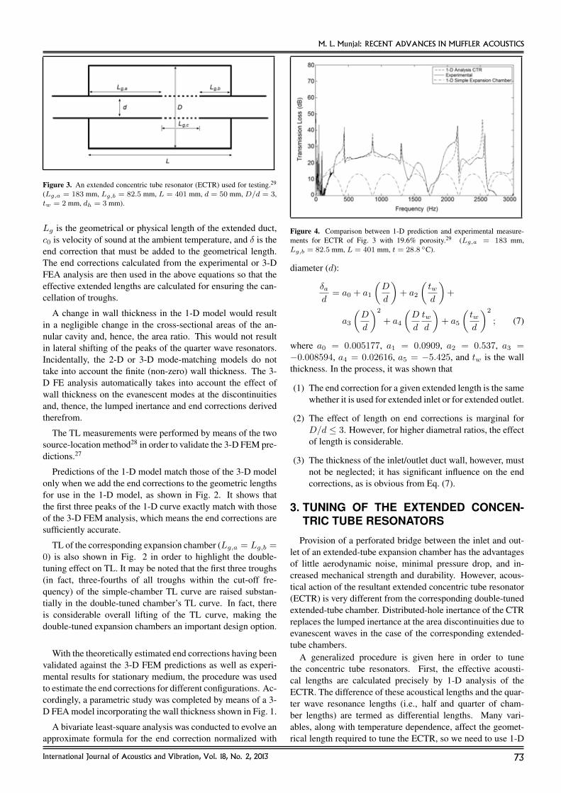
M. L. Munjal: RECENT ADVANCES IN MUFFLER ACOUSTICS
Figure 3. An extended concentric tube resonator (ECTR) used for testing.29
(Lg,a = 183 mm, Lg,b = 82.5 mm, L = 401 mm, d = 50 mm, D/d = 3,tw = 2 mm, dh = 3 mm).
Lg is the geometrical or physical length of the extended duct,c0 is velocity of sound at the ambient temperature, and δ is theend correction that must be added to the geometrical length.The end corrections calculated from the experimental or 3-DFEA analysis are then used in the above equations so that theeffective extended lengths are calculated for ensuring the can-cellation of troughs.
A change in wall thickness in the 1-D model would resultin a negligible change in the cross-sectional areas of the an-nular cavity and, hence, the area ratio. This would not resultin lateral shifting of the peaks of the quarter wave resonators.Incidentally, the 2-D or 3-D mode-matching models do nottake into account the finite (non-zero) wall thickness. The 3-D FE analysis automatically takes into account the effect ofwall thickness on the evanescent modes at the discontinuitiesand, thence, the lumped inertance and end corrections derivedtherefrom.
The TL measurements were performed by means of the twosource-location method28 in order to validate the 3-D FEM pre-dictions.27
Predictions of the 1-D model match those of the 3-D modelonly when we add the end corrections to the geometric lengthsfor use in the 1-D model, as shown in Fig. 2. It shows thatthe first three peaks of the 1-D curve exactly match with thoseof the 3-D FEM analysis, which means the end corrections aresufficiently accurate.
TL of the corresponding expansion chamber (Lg,a = Lg,b =0) is also shown in Fig. 2 in order to highlight the double-tuning effect on TL. It may be noted that the first three troughs(in fact, three-fourths of all troughs within the cut-off fre-quency) of the simple-chamber TL curve are raised substan-tially in the double-tuned chamber’s TL curve. In fact, thereis considerable overall lifting of the TL curve, making thedouble-tuned expansion chambers an important design option.
With the theoretically estimated end corrections having beenvalidated against the 3-D FEM predictions as well as experi-mental results for stationary medium, the procedure was usedto estimate the end corrections for different configurations. Ac-cordingly, a parametric study was completed by means of a 3-D FEA model incorporating the wall thickness shown in Fig. 1.
A bivariate least-square analysis was conducted to evolve anapproximate formula for the end correction normalized with
Figure 4. Comparison between 1-D prediction and experimental measure-ments for ECTR of Fig. 3 with 19.6% porosity.29 (Lg,a = 183 mm,Lg,b = 82.5 mm, L = 401 mm, t = 28.8 ◦C).
diameter (d):
δad
= a0 + a1
(D
d
)+ a2
(twd
)+
a3
(D
d
)2
+ a4
(D
d
twd
)+ a5
(twd
)2
; (7)
where a0 = 0.005177, a1 = 0.0909, a2 = 0.537, a3 =−0.008594, a4 = 0.02616, a5 = −5.425, and tw is the wallthickness. In the process, it was shown that
(1) The end correction for a given extended length is the samewhether it is used for extended inlet or for extended outlet.
(2) The effect of length on end corrections is marginal forD/d ≤ 3. However, for higher diametral ratios, the effectof length is considerable.
(3) The thickness of the inlet/outlet duct wall, however, mustnot be neglected; it has significant influence on the endcorrections, as is obvious from Eq. (7).
3. TUNING OF THE EXTENDED CONCEN-TRIC TUBE RESONATORS
Provision of a perforated bridge between the inlet and out-let of an extended-tube expansion chamber has the advantagesof little aerodynamic noise, minimal pressure drop, and in-creased mechanical strength and durability. However, acous-tical action of the resultant extended concentric tube resonator(ECTR) is very different from the corresponding double-tunedextended-tube chamber. Distributed-hole inertance of the CTRreplaces the lumped inertance at the area discontinuities due toevanescent waves in the case of the corresponding extended-tube chambers.
A generalized procedure is given here in order to tunethe concentric tube resonators. First, the effective acousti-cal lengths are calculated precisely by 1-D analysis of theECTR. The difference of these acoustical lengths and the quar-ter wave resonance lengths (i.e., half and quarter of cham-ber lengths) are termed as differential lengths. Many vari-ables, along with temperature dependence, affect the geomet-rical length required to tune the ECTR, so we need to use 1-D
International Journal of Acoustics and Vibration, Vol. 18, No. 2, 2013 73
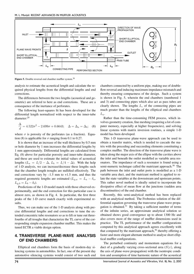
M. L. Munjal: RECENT ADVANCES IN MUFFLER ACOUSTICS
Figure 5. Double reversal end chamber muffler system.30
analysis to estimate the acoustical length and calculate the re-quired physical lengths from the differential lengths and endcorrections.
The differences between the two lengths (acoustical and ge-ometric) are referred to here as end corrections. These are aconsequence of the inertance of perforates.
The following least-squares fit has been developed for thedifferential length normalized with respect to the inner-tubediameter:29
∆
d= 4.522σ2 − 2.699σ + 0.6643; ∆ = ∆a = ∆b; (8)
where σ is porosity of the perforates (as a fraction). Equa-tion (8) is applicable for σ ranging from 0.1 to 0.27.
It is shown that an increase of the wall thickness by 0.5 mmor hole diameter by 1 mm increases the differential lengths by1 mm approximately. Differential lengths are calculated fromEq. (8) above for particular porosity and inner-tube diameter,and these are used to estimate the initial values of acousticallengths (La = L/2 − ∆, Lb = L/4 − ∆). With the helpof 1-D analysis, we can increase/decrease these lengths suchthat the chamber length troughs are nullified effectively. Theend corrections vary by –1.5 mm to +1.5 mm, and thus therequired geometric lengths are estimated (Lg,a = La − δa,Lg,b = Lb − δb).
Predictions of the 1-D model match with those observed ex-perimentally, and the end correction for this particular case isalmost zero, as shown in Fig. 4. In particular, the first threepeaks of the 1-D curve match exactly with experimental re-sults.
Thus, we can make use of the 1-D analysis along with pre-cise differential lengths and end corrections to tune the ex-tended concentric tube resonators so as to lift or tune out three-fourths of all troughs that characterize the TL curve of the cor-responding simple expansion chamber muffler. This makes thetuned ECTR a viable design option.
4. TRANSVERSE PLANE-WAVE ANALYSISOF END CHAMBERS
Elliptical end chambers form the basis of modern-day si-lencing systems in automobiles. In fact, one of the present dayautomotive silencing systems would consist of two such end
chambers connected by a uniform pipe, making use of double-flow reversal and inducing maximum impedance mismatch andthereby ensuring compactness of the design. Such a systemis shown in Fig. 5, wherein the end chambers (numbered 1and 3) and connecting pipes which also act as pass tubes areclearly shown. The lengths Lc of the connecting pipes aremuch greater than the lengths of the elliptical end chambersLa.
Rather than the time-consuming FEM process, which in-volves geometry creation, fine meshing (requiring a lot of com-puter memory, especially at higher frequencies), and solvinglinear systems with matrix inversion routines, a simple 1-Dmodel has been developed.
This 1-D transverse plane-wave approach can be used toobtain a transfer matrix, which is needed to cascade the ma-trix with the preceding and succeeding elements constituting acomplex muffler. The direction of the transverse plane wave istaken along the major axis of the ellipse with the cavities abovethe inlet and beneath the outlet modelled as variable area res-onators. The impedance of such a resonator is found using asemi-numeric technique called the matrizant approach.30 Thepath between the inlet and outlet ports is modelled as a 1-Dvariable area duct, and the matrizant method is applied to re-late the state variables at the downstream and upstream points.This rather novel method is ideally suited to incorporate thedissipative effect of mean flow at the junctions (sudden areadiscontinuities) of the end chamber.
Recently, this semi-analytical method has been replacedwith an analytical method. The Frobenius solution of the dif-ferential equation governing the transverse plane-wave propa-gation is obtained.31 By taking a sufficient number of termsof the infinite series, an approximate analytical solution soobtained shows good convergence up to about 1300 Hz andalso covers most of the range of muffler dimensions used inpractice. The TL performance of the muffler configurationscomputed by this analytical approach agrees excellently withthat computed by the matrizant approach,30 thereby offering afaster and more elegant alternate method to analyse short ellip-tical muffler configurations.
The perturbed continuity and momentum equations for aduct of a gradually varying cross-sectional area (S(x), alongthe axis of plane-wave propagation) with the isentropic condi-tion and assumption of time harmonic nature of the acoustical
74 International Journal of Acoustics and Vibration, Vol. 18, No. 2, 2013

M. L. Munjal: RECENT ADVANCES IN MUFFLER ACOUSTICS
Figure 6. An elliptical cross-section having a major diameter asD1 and minordiameter as D2. The distance x and non-dimensional length y is measuredfrom the top section S-S.31
Figure 7. A short elliptical chamber with a side inlet and (a) an end outlet porton the same half as the side inlet port and (b) an end outlet port on the oppositehalf of the side port.31
pressure field yield the following 1-D equation for acousticalwave propagation:14
d2p
dx2+ 1/S(x)(dS(x)/dx)
dp
dx+ k20p = 0. (9)
The assumption of a stationary medium (i.e., the mean flowMach number, M = 0) with no viscous losses is inherent inthe derivation of Eq. (9). The cross-sectional area S(x) forpropagation along the transverse direction in a short ellipticalchamber is given as31
S(x) = (2D2L/D1)(√
D1x− x2)
;
⇓
S(y) = (2D2L)(√
y − y2)
; y = x/D1. (10)
Figure 8. A short elliptical chamber with an end inlet and end outlet port withboth the ports located (a) on the same half and (b) on the opposite halves.31
In Eq. (10), D2 is the minor axis of the elliptical section, andL is the axial length of the chamber. The coordinate x is beingmeasured from the top of the elliptical chamber as depicted inFig. 6, while y is the non-dimensional counterpart of x. Theregion of interest where we look for a solution of Eq. (9) is 0 ≤x ≤ D1, and in a non-dimensional form, we get 0 ≤ y ≤ 1.By making use of Eq. (10), we get a non-dimensional form ofEq. (9) as
d2p
dy2+((1/2− y)/(y − y2)
) dpdy
+ β2p = 0; β = k0D1.
(11)It is interesting to note that by replacing y with 1−z, such that(0 ≤ z ≤ 1) in Eq. (11), the differential equation so obtainedhas the same form as Eq. (11), as shown below:
d2p
dz2+((1/2− z)/(z − z2)
) dpdz
+ β2p = 0; β = k0D1.
(12)Hence, Eqs. (11) and (12) reveal the symmetry of the solutionabout y = 0.5 or equivalently about x = D1/2. Thus, wemust solve Eq. (11) for the region 0 ≤ y ≤ 1/2 only, as thesolution for the other half (i.e., Eq. (12) is the same as that ob-tained by solving Eq. (11)). In fact, we exploit this symmetryproperty of the differential equation governing the transversewave propagation in elliptic ducts to find the Frobenius solu-tion of Eq. (11), computing only as many terms as would giveus a satisfactory convergence up to y ≤ 0.5. It is importantto take note of the singular points of Eq. (11) before attempt-ing the series solution. Some typical muffler configurations ofshort elliptical end chambers are shown in Figs. 7 and 8. Vali-dation of the transverse plane wave approach using Frobeniussolution is provided in Fig. 9.
It is indeed observed that this analytical approach31 is much
International Journal of Acoustics and Vibration, Vol. 18, No. 2, 2013 75
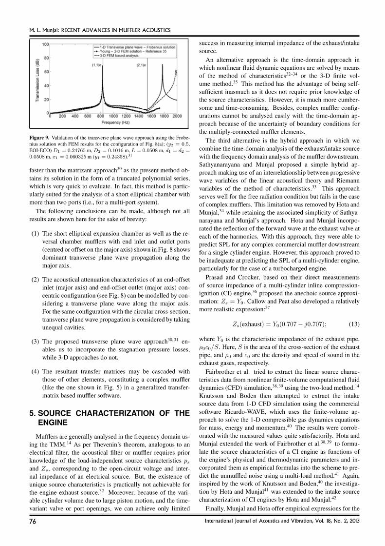
M. L. Munjal: RECENT ADVANCES IN MUFFLER ACOUSTICS
Figure 9. Validation of the transverse plane wave approach using the Frobe-nius solution with FEM results for the configuration of Fig. 8(a); (y2 = 0.5,EOI-ECO) D1 = 0.24765 m, D2 = 0.1016 m, L = 0.0508 m, d1 = d2 =0.0508 m, x1 = 0.060325 m (y1 = 0.24358).31
faster than the matrizant approach30 as the present method ob-tains its solution in the form of a truncated polynomial series,which is very quick to evaluate. In fact, this method is partic-ularly suited for the analysis of a short elliptical chamber withmore than two ports (i.e., for a multi-port system).
The following conclusions can be made, although not allresults are shown here for the sake of brevity:
(1) The short elliptical expansion chamber as well as the re-versal chamber mufflers with end inlet and outlet ports(centred or offset on the major axis) shown in Fig. 8 showsdominant transverse plane wave propagation along themajor axis.
(2) The acoustical attenuation characteristics of an end-offsetinlet (major axis) and end-offset outlet (major axis) con-centric configuration (see Fig. 8) can be modelled by con-sidering a transverse plane wave along the major axis.For the same configuration with the circular cross-section,transverse plane wave propagation is considered by takingunequal cavities.
(3) The proposed transverse plane wave approach30, 31 en-ables us to incorporate the stagnation pressure losses,while 3-D approaches do not.
(4) The resultant transfer matrices may be cascaded withthose of other elements, constituting a complex muffler(like the one shown in Fig. 5) in a generalized transfer-matrix based muffler software.
5. SOURCE CHARACTERIZATION OF THEENGINE
Mufflers are generally analysed in the frequency domain us-ing the TMM.14 As per Thevenin’s theorem, analogous to anelectrical filter, the acoustical filter or muffler requires priorknowledge of the load-independent source characteristics psand Zs, corresponding to the open-circuit voltage and inter-nal impedance of an electrical source. But, the existence ofunique source characteristics is practically not achievable forthe engine exhaust source.32 Moreover, because of the vari-able cylinder volume due to large piston motion, and the time-variant valve or port openings, we can achieve only limited
success in measuring internal impedance of the exhaust/intakesource.
An alternative approach is the time-domain approach inwhich nonlinear fluid dynamic equations are solved by meansof the method of characteristics32–34 or the 3-D finite vol-ume method.35 This method has the advantage of being self-sufficient inasmuch as it does not require prior knowledge ofthe source characteristics. However, it is much more cumber-some and time-consuming. Besides, complex muffler config-urations cannot be analysed easily with the time-domain ap-proach because of the uncertainty of boundary conditions forthe multiply-connected muffler elements.
The third alternative is the hybrid approach in which wecombine the time-domain analysis of the exhaust/intake sourcewith the frequency domain analysis of the muffler downstream.Sathyanarayana and Munjal proposed a simple hybrid ap-proach making use of an interrelationship between progressivewave variables of the linear acoustical theory and Riemannvariables of the method of characteristics.33 This approachserves well for the free radiation condition but fails in the caseof complex mufflers. This limitation was removed by Hota andMunjal,34 while retaining the associated simplicity of Sathya-narayana and Munjal’s approach. Hota and Munjal incorpo-rated the reflection of the forward wave at the exhaust valve ateach of the harmonics. With this approach, they were able topredict SPL for any complex commercial muffler downstreamfor a single cylinder engine. However, this approach proved tobe inadequate at predicting the SPL of a multi-cylinder engine,particularly for the case of a turbocharged engine.
Prasad and Crocker, based on their direct measurementsof source impedance of a multi-cylinder inline compression-ignition (CI) engine,36 proposed the anechoic source approxi-mation: Zs = Y0. Callow and Peat also developed a relativelymore realistic expression:37
Zs(exhaust) = Y0(0.707− j0.707); (13)
where Y0 is the characteristic impedance of the exhaust pipe,ρ0c0/S. Here, S is the area of the cross-section of the exhaustpipe, and ρ0 and c0 are the density and speed of sound in theexhaust gases, respectively.
Fairbrother et al. tried to extract the linear source charac-teristics data from nonlinear finite-volume computational fluiddynamics (CFD) simulation,38, 39 using the two-load method.14
Knutsson and Boden then attempted to extract the intakesource data from 1-D CFD simulation using the commercialsoftware Ricardo-WAVE, which uses the finite-volume ap-proach to solve the 1-D compressible gas dynamics equationsfor mass, energy and momentum.40 The results were corrob-orated with the measured values quite satisfactorily. Hota andMunjal extended the work of Fairbrother et al.38, 39 to formu-late the source characteristics of a CI engine as functions ofthe engine’s physical and thermodynamic parameters and in-corporated them as empirical formulas into the scheme to pre-dict the unmuffled noise using a multi-load method.41 Again,inspired by the work of Knutsson and Boden,40 the investiga-tion by Hota and Munjal41 was extended to the intake sourcecharacterization of CI engines by Hota and Munjal.42
Finally, Munjal and Hota offer empirical expressions for the
76 International Journal of Acoustics and Vibration, Vol. 18, No. 2, 2013
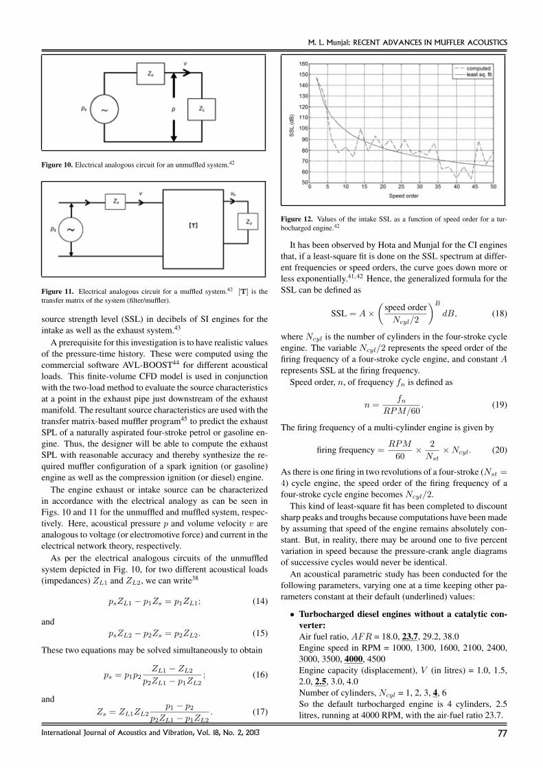
M. L. Munjal: RECENT ADVANCES IN MUFFLER ACOUSTICS
Figure 10. Electrical analogous circuit for an unmuffled system.42
Figure 11. Electrical analogous circuit for a muffled system.42 [T] is thetransfer matrix of the system (filter/muffler).
source strength level (SSL) in decibels of SI engines for theintake as well as the exhaust system.43
A prerequisite for this investigation is to have realistic valuesof the pressure-time history. These were computed using thecommercial software AVL-BOOST44 for different acousticalloads. This finite-volume CFD model is used in conjunctionwith the two-load method to evaluate the source characteristicsat a point in the exhaust pipe just downstream of the exhaustmanifold. The resultant source characteristics are used with thetransfer matrix-based muffler program45 to predict the exhaustSPL of a naturally aspirated four-stroke petrol or gasoline en-gine. Thus, the designer will be able to compute the exhaustSPL with reasonable accuracy and thereby synthesize the re-quired muffler configuration of a spark ignition (or gasoline)engine as well as the compression ignition (or diesel) engine.
The engine exhaust or intake source can be characterizedin accordance with the electrical analogy as can be seen inFigs. 10 and 11 for the unmuffled and muffled system, respec-tively. Here, acoustical pressure p and volume velocity v areanalogous to voltage (or electromotive force) and current in theelectrical network theory, respectively.
As per the electrical analogous circuits of the unmuffledsystem depicted in Fig. 10, for two different acoustical loads(impedances) ZL1 and ZL2, we can write38
psZL1 − p1Zs = p1ZL1; (14)
andpsZL2 − p2Zs = p2ZL2. (15)
These two equations may be solved simultaneously to obtain
ps = p1p2ZL1 − ZL2
p2ZL1 − p1ZL2; (16)
andZs = ZL1ZL2
p1 − p2p2ZL1 − p1ZL2
. (17)
Figure 12. Values of the intake SSL as a function of speed order for a tur-bocharged engine.42
It has been observed by Hota and Munjal for the CI enginesthat, if a least-square fit is done on the SSL spectrum at differ-ent frequencies or speed orders, the curve goes down more orless exponentially.41, 42 Hence, the generalized formula for theSSL can be defined as
SSL = A×(
speed orderNcyl/2
)B
dB, (18)
where Ncyl is the number of cylinders in the four-stroke cycleengine. The variable Ncyl/2 represents the speed order of thefiring frequency of a four-stroke cycle engine, and constant Arepresents SSL at the firing frequency.
Speed order, n, of frequency fn is defined as
n =fn
RPM/60. (19)
The firing frequency of a multi-cylinder engine is given by
firing frequency =RPM
60× 2
Nst×Ncyl. (20)
As there is one firing in two revolutions of a four-stroke (Nst =4) cycle engine, the speed order of the firing frequency of afour-stroke cycle engine becomes Ncyl/2.
This kind of least-square fit has been completed to discountsharp peaks and troughs because computations have been madeby assuming that speed of the engine remains absolutely con-stant. But, in reality, there may be around one to five percentvariation in speed because the pressure-crank angle diagramsof successive cycles would never be identical.
An acoustical parametric study has been conducted for thefollowing parameters, varying one at a time keeping other pa-rameters constant at their default (underlined) values:
• Turbocharged diesel engines without a catalytic con-verter:Air fuel ratio, AFR = 18.0, 23.7, 29.2, 38.0Engine speed in RPM = 1000, 1300, 1600, 2100, 2400,3000, 3500, 4000, 4500Engine capacity (displacement), V (in litres) = 1.0, 1.5,2.0, 2.5, 3.0, 4.0Number of cylinders, Ncyl = 1, 2, 3, 4, 6So the default turbocharged engine is 4 cylinders, 2.5litres, running at 4000 RPM, with the air-fuel ratio 23.7.
International Journal of Acoustics and Vibration, Vol. 18, No. 2, 2013 77
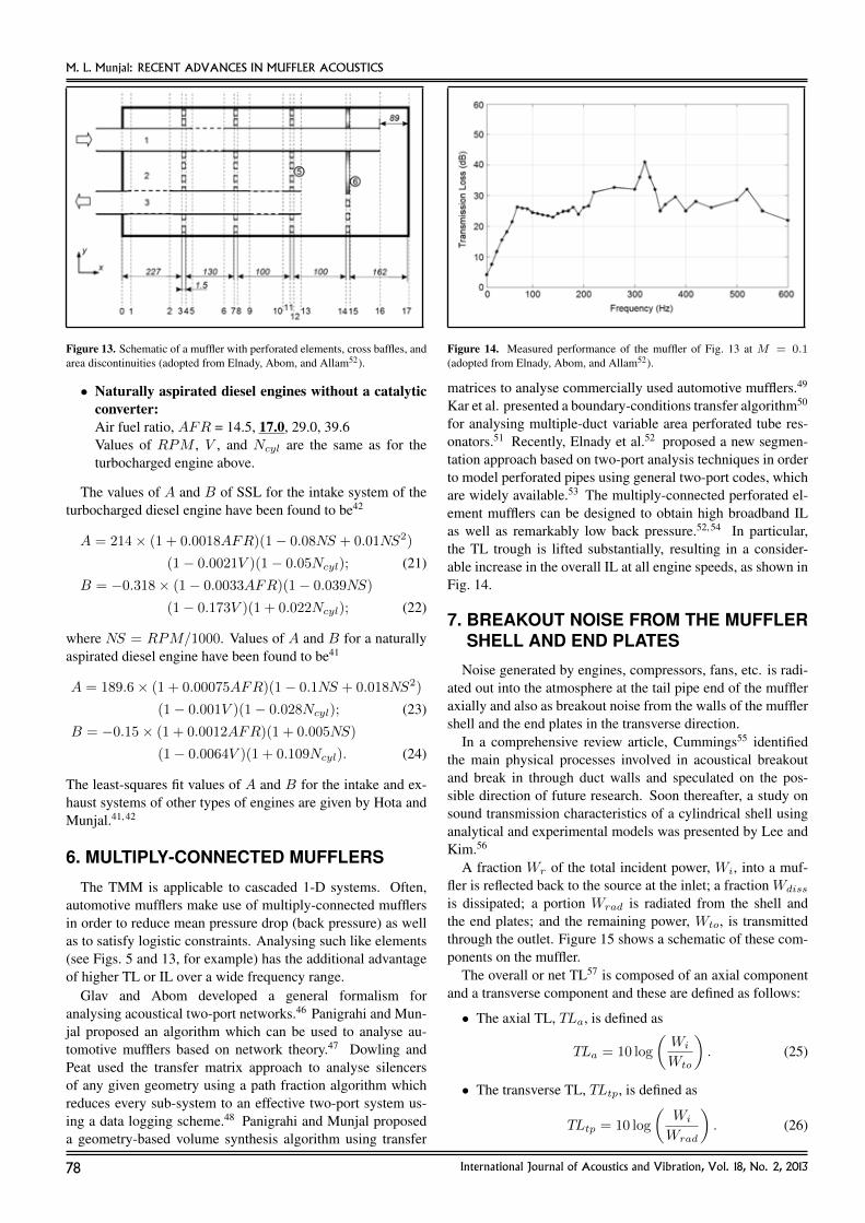
M. L. Munjal: RECENT ADVANCES IN MUFFLER ACOUSTICS
Figure 13. Schematic of a muffler with perforated elements, cross baffles, andarea discontinuities (adopted from Elnady, Abom, and Allam52).
• Naturally aspirated diesel engines without a catalyticconverter:Air fuel ratio, AFR = 14.5, 17.0, 29.0, 39.6Values of RPM , V , and Ncyl are the same as for theturbocharged engine above.
The values of A and B of SSL for the intake system of theturbocharged diesel engine have been found to be42
A = 214× (1 + 0.0018AFR)(1− 0.08NS + 0.01NS2)
(1− 0.0021V )(1− 0.05Ncyl); (21)
B = −0.318× (1− 0.0033AFR)(1− 0.039NS)
(1− 0.173V )(1 + 0.022Ncyl); (22)
where NS = RPM/1000. Values of A and B for a naturallyaspirated diesel engine have been found to be41
A = 189.6× (1 + 0.00075AFR)(1− 0.1NS + 0.018NS2)
(1− 0.001V )(1− 0.028Ncyl); (23)
B = −0.15× (1 + 0.0012AFR)(1 + 0.005NS)
(1− 0.0064V )(1 + 0.109Ncyl). (24)
The least-squares fit values of A and B for the intake and ex-haust systems of other types of engines are given by Hota andMunjal.41, 42
6. MULTIPLY-CONNECTED MUFFLERS
The TMM is applicable to cascaded 1-D systems. Often,automotive mufflers make use of multiply-connected mufflersin order to reduce mean pressure drop (back pressure) as wellas to satisfy logistic constraints. Analysing such like elements(see Figs. 5 and 13, for example) has the additional advantageof higher TL or IL over a wide frequency range.
Glav and Abom developed a general formalism foranalysing acoustical two-port networks.46 Panigrahi and Mun-jal proposed an algorithm which can be used to analyse au-tomotive mufflers based on network theory.47 Dowling andPeat used the transfer matrix approach to analyse silencersof any given geometry using a path fraction algorithm whichreduces every sub-system to an effective two-port system us-ing a data logging scheme.48 Panigrahi and Munjal proposeda geometry-based volume synthesis algorithm using transfer
Figure 14. Measured performance of the muffler of Fig. 13 at M = 0.1(adopted from Elnady, Abom, and Allam52).
matrices to analyse commercially used automotive mufflers.49
Kar et al. presented a boundary-conditions transfer algorithm50
for analysing multiple-duct variable area perforated tube res-onators.51 Recently, Elnady et al.52 proposed a new segmen-tation approach based on two-port analysis techniques in orderto model perforated pipes using general two-port codes, whichare widely available.53 The multiply-connected perforated el-ement mufflers can be designed to obtain high broadband ILas well as remarkably low back pressure.52, 54 In particular,the TL trough is lifted substantially, resulting in a consider-able increase in the overall IL at all engine speeds, as shown inFig. 14.
7. BREAKOUT NOISE FROM THE MUFFLERSHELL AND END PLATES
Noise generated by engines, compressors, fans, etc. is radi-ated out into the atmosphere at the tail pipe end of the muffleraxially and also as breakout noise from the walls of the mufflershell and the end plates in the transverse direction.
In a comprehensive review article, Cummings55 identifiedthe main physical processes involved in acoustical breakoutand break in through duct walls and speculated on the pos-sible direction of future research. Soon thereafter, a study onsound transmission characteristics of a cylindrical shell usinganalytical and experimental models was presented by Lee andKim.56
A fraction Wr of the total incident power, Wi, into a muf-fler is reflected back to the source at the inlet; a fraction Wdiss
is dissipated; a portion Wrad is radiated from the shell andthe end plates; and the remaining power, Wto, is transmittedthrough the outlet. Figure 15 shows a schematic of these com-ponents on the muffler.
The overall or net TL57 is composed of an axial componentand a transverse component and these are defined as follows:
• The axial TL, TLa, is defined as
TLa = 10 log
(Wi
Wto
). (25)
• The transverse TL, TLtp, is defined as
TLtp = 10 log
(Wi
Wrad
). (26)
78 International Journal of Acoustics and Vibration, Vol. 18, No. 2, 2013
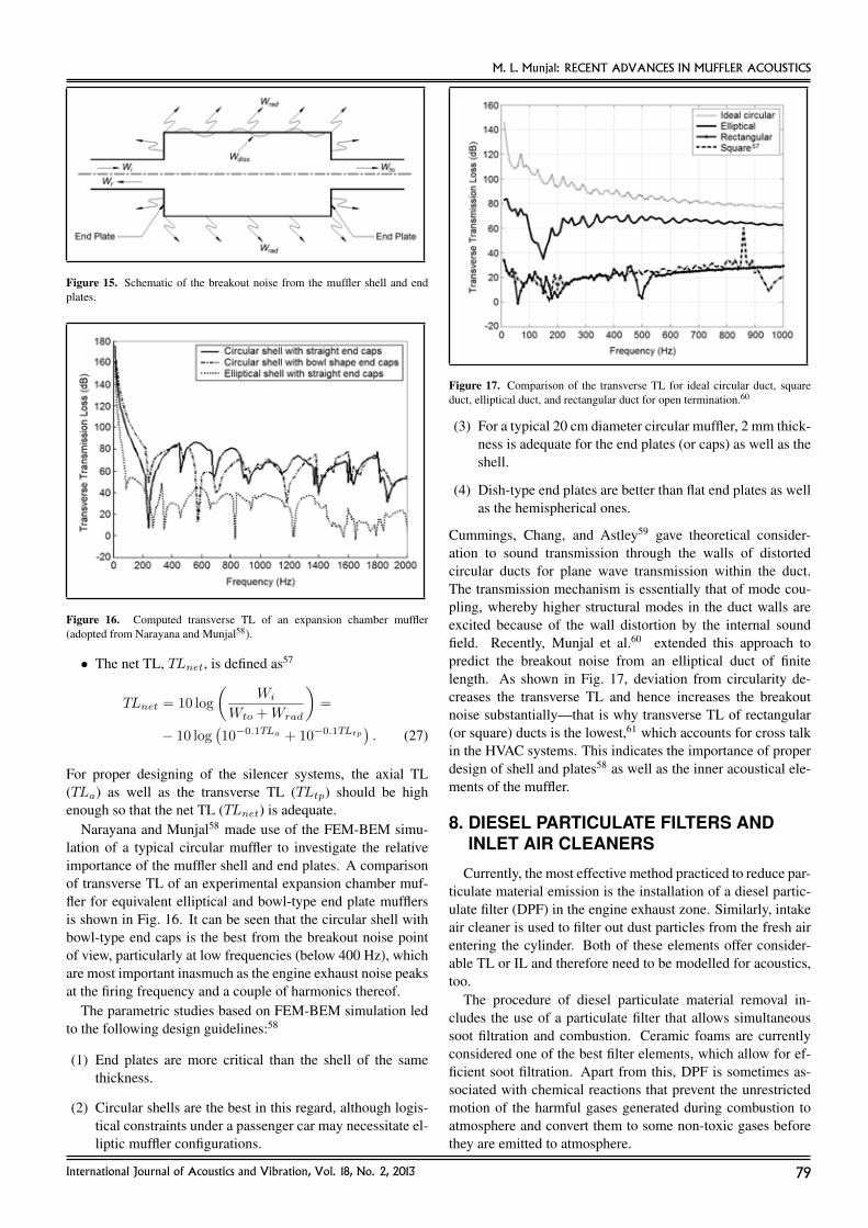
M. L. Munjal: RECENT ADVANCES IN MUFFLER ACOUSTICS
Figure 15. Schematic of the breakout noise from the muffler shell and endplates.
Figure 16. Computed transverse TL of an expansion chamber muffler(adopted from Narayana and Munjal58).
• The net TL, TLnet, is defined as57
TLnet = 10 log
(Wi
Wto +Wrad
)=
− 10 log(10−0.1TLa + 10−0.1TLtp
). (27)
For proper designing of the silencer systems, the axial TL(TLa) as well as the transverse TL (TLtp) should be highenough so that the net TL (TLnet) is adequate.
Narayana and Munjal58 made use of the FEM-BEM simu-lation of a typical circular muffler to investigate the relativeimportance of the muffler shell and end plates. A comparisonof transverse TL of an experimental expansion chamber muf-fler for equivalent elliptical and bowl-type end plate mufflersis shown in Fig. 16. It can be seen that the circular shell withbowl-type end caps is the best from the breakout noise pointof view, particularly at low frequencies (below 400 Hz), whichare most important inasmuch as the engine exhaust noise peaksat the firing frequency and a couple of harmonics thereof.
The parametric studies based on FEM-BEM simulation ledto the following design guidelines:58
(1) End plates are more critical than the shell of the samethickness.
(2) Circular shells are the best in this regard, although logis-tical constraints under a passenger car may necessitate el-liptic muffler configurations.
Figure 17. Comparison of the transverse TL for ideal circular duct, squareduct, elliptical duct, and rectangular duct for open termination.60
(3) For a typical 20 cm diameter circular muffler, 2 mm thick-ness is adequate for the end plates (or caps) as well as theshell.
(4) Dish-type end plates are better than flat end plates as wellas the hemispherical ones.
Cummings, Chang, and Astley59 gave theoretical consider-ation to sound transmission through the walls of distortedcircular ducts for plane wave transmission within the duct.The transmission mechanism is essentially that of mode cou-pling, whereby higher structural modes in the duct walls areexcited because of the wall distortion by the internal soundfield. Recently, Munjal et al.60 extended this approach topredict the breakout noise from an elliptical duct of finitelength. As shown in Fig. 17, deviation from circularity de-creases the transverse TL and hence increases the breakoutnoise substantially—that is why transverse TL of rectangular(or square) ducts is the lowest,61 which accounts for cross talkin the HVAC systems. This indicates the importance of properdesign of shell and plates58 as well as the inner acoustical ele-ments of the muffler.
8. DIESEL PARTICULATE FILTERS ANDINLET AIR CLEANERS
Currently, the most effective method practiced to reduce par-ticulate material emission is the installation of a diesel partic-ulate filter (DPF) in the engine exhaust zone. Similarly, intakeair cleaner is used to filter out dust particles from the fresh airentering the cylinder. Both of these elements offer consider-able TL or IL and therefore need to be modelled for acoustics,too.
The procedure of diesel particulate material removal in-cludes the use of a particulate filter that allows simultaneoussoot filtration and combustion. Ceramic foams are currentlyconsidered one of the best filter elements, which allow for ef-ficient soot filtration. Apart from this, DPF is sometimes as-sociated with chemical reactions that prevent the unrestrictedmotion of the harmful gases generated during combustion toatmosphere and convert them to some non-toxic gases beforethey are emitted to atmosphere.
International Journal of Acoustics and Vibration, Vol. 18, No. 2, 2013 79
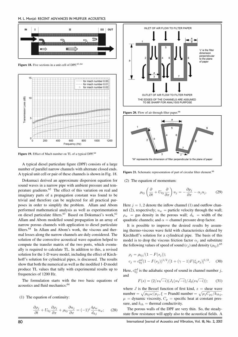
M. L. Munjal: RECENT ADVANCES IN MUFFLER ACOUSTICS
Figure 18. Five sections in a unit cell of DPF.63, 64
Figure 19. Effect of Mach number on TL of a typical DPF.64
A typical diesel particulate figure (DPF) consists of a largenumber of parallel narrow channels with alternate closed ends.A typical unit cell or pair of these channels is shown in Fig. 18.
Dokumaci derived an approximate dispersion equation forsound waves in a narrow pipe with ambient pressure and tem-perature gradients.62 The effect of this variation on real andimaginary parts of a propagation constant was found to betrivial and therefore can be neglected for all practical pur-poses in order to simplify the problem. Allam and Abomperformed mathematical analysis as well as experimentationon diesel particulate filters.63 Based on Dokumaci’s work,62
Allam and Abom modelled sound propagation in an array ofnarrow porous channels with application to diesel particulatefilters.64 In Allam and Abom’s work, the viscous and ther-mal losses along the narrow channels are duly considered. Thesolution of the convective acoustical wave equation helped tocompute the transfer matrix of the two ports, which eventu-ally is required to calculate TL. In addition to this, a revisedsolution for the 1-D wave model, including the effect of Kirch-hoff’s solution for cylindrical pipes, is discussed. The resultsshow that both the numerical as well as the modified 1-D modelproduce TL values that tally with experimental results up tofrequencies of 1200 Hz.
The formulation starts with the two basic equations ofacoustics and fluid mechanics:64
(1) The equation of continuity:
∂ρj∂t
+ U0j∂ρj∂x
+ ρ0j∂uj∂x
= (−1)j4ρwdhj
uw; (28)
Figure 20. Flow of air through filter paper.66
Figure 21. Schematic representation of part of circular filter element.66
(2) The equation of momentum:
ρ0j
(∂
∂t+ U0j
∂
∂x
)uj = −∂pj
∂x− αjuj . (29)
Here j = 1, 2 denote the inflow channel (1) and outflow chan-nel (2), respectively; uw = particle velocity through the wall;ρw = gas density in the porous wall; dh = width of thequadratic channels; and α = channel pressure drop factor.
It is possible to improve the desired results by assum-ing thermo-viscous wave field with characteristics defined byKirchhoff’s solution for a cylindrical pipe. The basis of thismodel is to drop the viscous friction factor αj and substitutethe following values of speed of sound (cj) and density (ρ0j):65
ρj = ρ0j/(1− F (sj));
cj = cad0j (1− F (sj))1/2/[1 + (γ − 1)F (ξjsj)]
1/2. (30)
Here, cad0j is the adiabatic speed of sound in channel number j,and
F (s) = (2/s√−i)(J1(s
√−i)/J0(s
√−i)); (31)
where J is the Bessel function of first kind, s = shear wavenumber =
√ρ0jω/µj , ξ = Prandtl number =
õjCpj/kthj ,
µ = dynamic viscosity, Cp = specific heat at constant pres-sure, and kth = thermal conductivity.
The porous walls of the DPF are very thin. So, the steady-state flow resistance will apply also to the acoustical fields. A
80 International Journal of Acoustics and Vibration, Vol. 18, No. 2, 2013
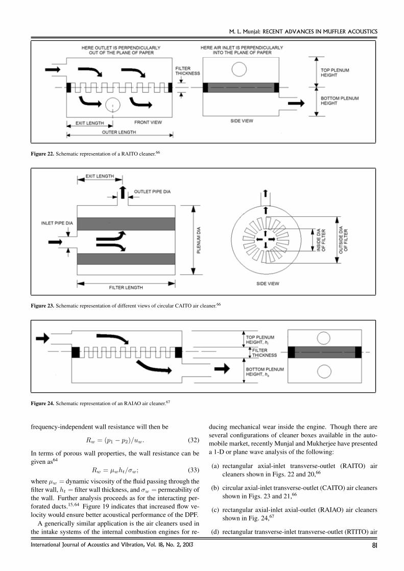
M. L. Munjal: RECENT ADVANCES IN MUFFLER ACOUSTICS
Figure 22. Schematic representation of a RAITO cleaner.66
Figure 23. Schematic representation of different views of circular CAITO air cleaner.66
Figure 24. Schematic representation of an RAIAO air cleaner.67
frequency-independent wall resistance will then be
Rw = (p1 − p2)/uw. (32)
In terms of porous wall properties, the wall resistance can begiven as64
Rw = µwht/σw; (33)
where µw = dynamic viscosity of the fluid passing through thefilter wall, ht = filter wall thickness, and σw = permeability ofthe wall. Further analysis proceeds as for the interacting per-forated ducts.15, 64 Figure 19 indicates that increased flow ve-locity would ensure better acoustical performance of the DPF.
A generically similar application is the air cleaners used inthe intake systems of the internal combustion engines for re-
ducing mechanical wear inside the engine. Though there areseveral configurations of cleaner boxes available in the auto-mobile market, recently Munjal and Mukherjee have presenteda 1-D or plane wave analysis of the following:
(a) rectangular axial-inlet transverse-outlet (RAITO) aircleaners shown in Figs. 22 and 20,66
(b) circular axial-inlet transverse-outlet (CAITO) air cleanersshown in Figs. 23 and 21,66
(c) rectangular axial-inlet axial-outlet (RAIAO) air cleanersshown in Fig. 24,67
(d) rectangular transverse-inlet transverse-outlet (RTITO) air
International Journal of Acoustics and Vibration, Vol. 18, No. 2, 2013 81

M. L. Munjal: RECENT ADVANCES IN MUFFLER ACOUSTICS
cleaners shown in Fig. 25.67
The 1-D acoustical analysis model proposed by Munjal andMukherjee66, 67 makes use of an analogy to a two-duct perfo-rated cross flow element.7 Results of the 1-D analysis werevalidated with those of the 3-D finite element software SYS-NOISE.
In the RAITO filter cleaner shown in Fig. 22, the mean flowenters axially in the top plenum, passes through the filter ele-ment, and then exits the bottom plenum in the transverse di-rection. Typical thickness of the filtering element is around25 mm, and the paper that the filter is made of has a thick-ness of around 0.35–1 mm. The filter paper is treated as auniformly perforated element. However, since the filter con-figuration cannot be treated as a uniformly perforated elementin a single plane, we need to modify the resistance value of thetotal filter accordingly. This can be done as follows.
It is obvious from Fig. 20 that in this configuration, the flowgets more than one path to traverse from the top plenum to thebottom plenum, compared to a configuration in which the filterpaper would lie flat on a single plane without any waviness.For this reason, due to the special configuration of the filteringelement, we need to modify the nominal resistance of the filterpaper. To get an idea of how this modification can be done, inFig. 20, two open and three closed channels are drawn, but theanalysis is based on n pairs of such channels. The division offlow corresponds to resistances in parallel. Thus,
1/Req = (2n+ 1)/R1 + 2n/R2. (34)
Now,
Req =((p1 − p2)/uf )eq
(2n+ 1)ac;
R1 = (1/ac)(µh/σ);
R2 = (1/bc)(µh/σ); (35)
where p1 and p2 are acoustical pressures in the two regionsacross the filter element, uf is the surface averaged particlevelocity through the filter element, µ is dynamic viscosity ofair, h is filter paper thickness, σ is permeability of the filterpaper, and µh/σ is the resistance provided by the filter wall.68
Substituting all these values in Eq. (34) yields
ζ ≡ (p/u)eq = (µh/σ) [a/ {a+ 2n/(2n+ 1)b}] . (36)
In all practical cases, n is a large number (varying from 20–100). Therefore, 2n/(2n+ 1) ≈ 1. Thus,
ζ = (µh/σ) [a/(a+ b)] . (37)
Typical results of the analysis66, 67 are shown in Figs. 26 and27. The data assumed to generate these plots are as follows(see Fig. 22): Cleaner outer length = 275 mm; cleaner outerwidth = 170 mm; filter thickness = 20 mm; inside height ofthe top plenum = 60 mm; inside height of the bottom plenum= 60 mm; inlet pipe diameter = 40 mm; outlet pipe diameter= 40 mm; exit length = 137.5 mm; number of channel pairs =80 (approximately); filter paper permeability = 1×10⁻¹² m2
(range of permeability is obtained from Qi and Uesaka69).
Figure 25. Schematic representation of an RTITO air cleaner.67
Figure 26. Comparison of complete filter box effect with that of the plenumalone.66
Figure 26 brings out the role of the filter paper (the differ-ence between the two curves represents that effect). Resultsof the 1-D prediction model above are validated with the 3-D finite element predictions in Fig. 27, where the filter ele-ment is modeled by a transfer impedance interface condition((p1 − p2)/uf = µh/σ) between two neighbouring finite ele-ments.
It should be noted that up to 700 Hz, the 1-D model and 3-DFEM results are in good agreement with each other. Beyondthat frequency, two curves start deviating from each other.This is not a limitation since our main interest lies in the low-frequency zone, where the intake SPL is relatively high. Oneimportant note should be highlighted here. In Fig. 27, one res-onance peak is observed at 1000 Hz due to wave propagationin the y-direction in the configuration of Fig. 22. In our 1-Dmodel, considering wave propagation in the x-direction, wecannot capture this resonance peak in our TL versus frequencycurve. This is, of course, one of the limitations of this kind of1-D analytical formulation.
Similar inferences have been made for the RAIAO aircleaner of Fig. 24 and the RTITO air cleaner of Fig. 25.67
Major conclusions of this investigation are as follows:
(a) Typical inlet air cleaner acts as a simple expansion cham-ber. The filter element enhances its TL by means of inline
82 International Journal of Acoustics and Vibration, Vol. 18, No. 2, 2013
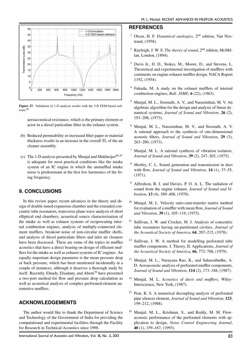
M. L. Munjal: RECENT ADVANCES IN MUFFLER ACOUSTICS
Figure 27. Validation of 1-D analysis results with the 3-D FEM-based soft-ware.66
aeroacoustical resistance, which is the primary element oractor in a diesel particulate filter in the exhaust system.
(b) Reduced permeability or increased filter paper or materialthickness results in an increase in the overall TL of the aircleaner assembly.
(c) The 1-D analysis presented by Munjal and Mukherjee66, 67
is adequate for most practical conditions like the intakesystem of an IC engine in which the unmuffled intakenoise is predominant at the first few harmonics of the fir-ing frequency.
9. CONCLUSIONS
In this review paper, recent advances in the theory and de-sign of double-tuned expansion chamber and the extended con-centric tube resonators, transverse plane wave analysis of shortelliptical end chambers, acoustical source characterization ofthe intake as well as exhaust systems of reciprocating inter-nal combustion engines, analysis of multiply-connected ele-ment mufflers, breakout noise of non-circular muffler shells,and analysis of diesel particulate filters and inlet air cleanershave been discussed. These are some of the topics in muffleracoustics that have a direct bearing on design of efficient muf-flers for the intake as well as exhaust systems of IC engines. Anequally important design parameter is the mean pressure dropor back pressure, which has been mentioned incidentally at acouple of instances, although it deserves a thorough study byitself. Recently, Elnady, Elsadany, and Abom70 have presenteda two-port method for flow and pressure drop calculation aswell as acoustical analysis of complex perforated-element au-tomotive mufflers.
ACKNOWLEDGEMENTS
The author would like to thank the Department of Scienceand Technology of the Government of India for providing thecomputational and experimental facilities through the Facilityfor Research in Technical Acoustics since 1998.
REFERENCES1 Olson, H. F. Dynamical analogies, 2nd edition, Van Nos-
trand, (1958).
2 Rayleigh, J. W. S. The theory of sound, 2nd edition, McMil-lan, London, (1894).
3 Davis Jr., D. D., Stokes, M., Moore, D., and Stevens, L.Theoretical and experimental investigation of mufflers withcomments on engine exhaust muffler design, NACA Report1192, (1954).
4 Fukuda, M. A study on the exhaust mufflers of internalcombustion engines, Bull. JSME, 6 (22), (1963).
5 Munjal, M. L., Sreenath, A. V., and Narasimhan, M. V. Analgebraic algorithm for the design and analysis of linear dy-namical systems, Journal of Sound and Vibration, 26 (2),193–208, (1973).
6 Munjal, M. L., Narasimhan, M. V., and Sreenath, A. V.A rational approach to the synthesis of one-dimensionalacoustic filters, Journal of Sound and Vibration, 29 (3),263–280, (1973).
7 Munjal, M. L. A rational synthesis of vibration isolators,Journal of Sound and Vibration, 39 (2), 247–265, (1975).
8 Morfey, C. L. Sound generation and transmission in ductwith flow, Journal of Sound and Vibration, 14 (1), 37–55,(1971).
9 Alfredson, R. J. and Davies, P. O. A. L. The radiation ofsound from the engine exhaust, Journal of Sound and Vi-bration, 13 (4), 389–408, (1970).
10 Munjal, M. L. Velocity ratio-cum-transfer matrix methodfor evaluation of a muffler with mean flow, Journal of Soundand Vibration, 39 (1), 105–119, (1975).
11 Sullivan, J. W. and Crocker, M. J. Analysis of concentrictube resonators having un-partitioned cavities, Journal ofthe Acoustical Society of America, 64, 207–215, (1978).
12 Sullivan, J. W. A method for modelling perforated tubemuffler components. I. Theory, II. Applications, Journal ofthe Acoustical Society of America, 66, 772–788, (1979).
13 Munjal, M. L., Narayana Rao, K., and Sahasrabudhe, A.D. Aeroacoustic analysis of perforated muffler components,Journal of Sound and Vibration, 114 (2), 173–188, (1987).
14 Munjal, M. L. Acoustics of ducts and mufflers, Wiley-Interscience, New York, (1987).
15 Peat, K. S. A numerical decoupling analysis of perforatedpipe silencer element, Journal of Sound and Vibration, 123,199–212, (1988).
16 Munjal, M. L., Krishnan, S., and Reddy, M. M. Flow-acoustic performance of the perforated elements with ap-plication to design, Noise Control Engineering Journal,40 (1), 159–167, (1993).
International Journal of Acoustics and Vibration, Vol. 18, No. 2, 2013 83

M. L. Munjal: RECENT ADVANCES IN MUFFLER ACOUSTICS
17 Gogate, G. R. and Munjal, M. L. Analytical and experimen-tal aeroacoustic studies of open-ended three-duct perforatedelements used in mufflers, Journal of the Acoustical Societyof America, 97 (5), 2919–2927, (1995).
18 Munjal, M. L. Plane wave analysis of side inlet/outletchamber mufflers with mean flow, Applied Acoustics,52 (2), 165–175, (1997).
19 Munjal, M. L., Behera, B. K., and Thawani, P. T. An ana-lytical model of the reverse flow, open end, extended per-forated element muffler, International Journal of Acousticsand Vibration, 2 (2), 59–62, (1997).
20 Munjal, M. L. Analysis of a flush tube three-pass perfo-rated element muffler by means of transfer matrices, Inter-national Journal of Acoustics and Vibration, 2 (2), 63–68,(1997).
21 Kar, T. and Munjal, M. L. Analysis and design of conicalconcentric tube resonators, Journal of the Acoustical Soci-ety of America, 116 (1), 74–83, (2004).
22 Kar, T. and Munjal, M. L. Generalized analysis of a mufflerwith any number of interacting ducts, Journal of Sound andVibration, 285 (3), 585–596, (2005).
23 Munjal, M. L., Galaitsis, A. G., and Ver, I. L. Passive si-lencers, In I. L. Ver and L. L. Beranek, eds., Noise and vi-bration control engineering, John Wiley, New York, (2006).
24 Munjal, M. L. Muffler acoustics, In F. P. Mechel, ed., For-mulas of acoustics, Springer Verlag, Berlin, (2002).
25 Munjal, M. L. and Gowri, S. Theory and design of tuned ex-tended tube chambers and concentric tube resonators, Jour-nal of the Acoustical Society of India, 36 (2), 53–71, (2009).
26 Karal, F. C. The analogous impedance for discontinuitiesand constrictions of circular cross-section, Journal of theAcoustical Society of America, 25 (2), 327–334, (1953).
27 Chaitanya, P. and Munjal, M. L. Effect of wall thicknesson the end corrections of the extended inlet and outletof a double-tuned expansion chamber, Applied Acoustics,72 (1), 65–70, (2011).
28 Munjal, M. L. and Doige, A. G. Theory of a two source-location method for direct experimental evaluation of thefour-pole parameters of an aeroacoustic element, Journalof Sound and Vibration, 141 (2), 323–334, (1990).
29 Chaitanya, P. and Munjal, M. L. Tuning of the ex-tended concentric tube resonators, SAE International Sym-posium on International Automotive Technology (SIAT-2011), 2011-26-0070, ARAI, Pune, India, (2011).
30 Mimani, A. and Munjal, M. L. Transverse plane-wave anal-ysis of short elliptical end-chamber and expansion-chambermufflers, International Journal of Acoustics and Vibration,15 (1), 24–38, (2010).
31 Mimani, A. and Munjal, M. L. Transverse plane wave anal-ysis of short elliptical chamber mufflers — An analyticalapproach, Journal of Sound and Vibration, 330, 1472–1489,(2011).
32 Gupta, V. H. and Munjal, M. L. On numerical predictionof the acoustical source characteristics of an engine ex-haust system, Journal of the Acoustical Society of America,92 (5), 2716–2725, (1992).
33 Sathyanarayana, Y. and Munjal, M. L. A hybrid approachfor aero-acoustic analysis of the engine exhaust system, Ap-plied Acoustics, 60, 425–450, (2000).
34 Hota, R. N. and Munjal, M. L. A new hybrid approach forthermo-acoustic modeling of engine exhaust system, Inter-national Journal of Acoustics and Vibration, 9 (3), 129–138, (2004).
35 Young, C.-I. J. and Crocker, M. J. Prediction of transmis-sion loss in mufflers by the finite element method, Jour-nal of the Acoustical Society of America, 57 (1), 144–148,(1975).
36 Prasad, M. G. and Crocker, M. J. On the measurement ofthe internal source impedance of a multi-cylinder engineexhaust system, Journal of Sound and Vibration, 90, 491–508, (1983).
37 Callow, G. D. and Peat, K. S. Insertion loss of engine inflowand exhaust silencers, I Mech. E C19/88:39-46, (1988).
38 Fairbrother, R., Boden, H., and Glav, R. Linear acoustic ex-haust system simulation using source data from linear sim-ulation, SAE Technical Paper 2005-01-2358, (2005).
39 Boden, H., Tonse M., and Fairbrother, R. On extractionof IC-engine acoustic source data from non-linear simula-tions, Proceedings of the Eleventh International Congresson Sound and Vibration (ICSV11), St. Petersburg, Russia,(2004).
40 Knutsson, M. and Boden, H. IC-Engine intake source datafrom non-linear simulations, SAE Technical Paper 2007-01-2209, (2007).
41 Hota, R. N. and Munjal, M. L. Approximate empirical ex-pressions for the aeroacoustic source strength level of theexhaust system of compression ignition engines, Interna-tional Journal of Aeroacoustics, 7 (3–4), 349–371, (2008).
42 Hota, R. N. and Munjal, M. L. Intake source characteriza-tion of a compression ignition engine: Empirical expres-sions, Noise Control Engineering Journal, 56 (2), 92–106,(2008).
43 Munjal, M. L. and Hota, R. N. Acoustic source character-istics of the exhaust and intake systems of a spark ignitionengine, Paper No. 78, Inter-Noise 2010, Lisbon, Portugal,(2010).
44 BOOST Version 5.0.2, AVL LIST GmbH, Graz, Austria,(2007).
84 International Journal of Acoustics and Vibration, Vol. 18, No. 2, 2013
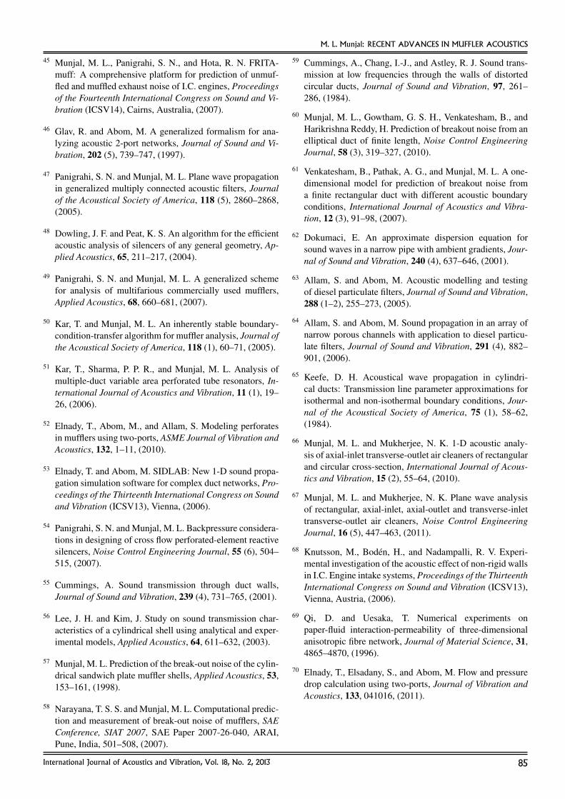
M. L. Munjal: RECENT ADVANCES IN MUFFLER ACOUSTICS
45 Munjal, M. L., Panigrahi, S. N., and Hota, R. N. FRITA-muff: A comprehensive platform for prediction of unmuf-fled and muffled exhaust noise of I.C. engines, Proceedingsof the Fourteenth International Congress on Sound and Vi-bration (ICSV14), Cairns, Australia, (2007).
46 Glav, R. and Abom, M. A generalized formalism for ana-lyzing acoustic 2-port networks, Journal of Sound and Vi-bration, 202 (5), 739–747, (1997).
47 Panigrahi, S. N. and Munjal, M. L. Plane wave propagationin generalized multiply connected acoustic filters, Journalof the Acoustical Society of America, 118 (5), 2860–2868,(2005).
48 Dowling, J. F. and Peat, K. S. An algorithm for the efficientacoustic analysis of silencers of any general geometry, Ap-plied Acoustics, 65, 211–217, (2004).
49 Panigrahi, S. N. and Munjal, M. L. A generalized schemefor analysis of multifarious commercially used mufflers,Applied Acoustics, 68, 660–681, (2007).
50 Kar, T. and Munjal, M. L. An inherently stable boundary-condition-transfer algorithm for muffler analysis, Journal ofthe Acoustical Society of America, 118 (1), 60–71, (2005).
51 Kar, T., Sharma, P. P. R., and Munjal, M. L. Analysis ofmultiple-duct variable area perforated tube resonators, In-ternational Journal of Acoustics and Vibration, 11 (1), 19–26, (2006).
52 Elnady, T., Abom, M., and Allam, S. Modeling perforatesin mufflers using two-ports, ASME Journal of Vibration andAcoustics, 132, 1–11, (2010).
53 Elnady, T. and Abom, M. SIDLAB: New 1-D sound propa-gation simulation software for complex duct networks, Pro-ceedings of the Thirteenth International Congress on Soundand Vibration (ICSV13), Vienna, (2006).
54 Panigrahi, S. N. and Munjal, M. L. Backpressure considera-tions in designing of cross flow perforated-element reactivesilencers, Noise Control Engineering Journal, 55 (6), 504–515, (2007).
55 Cummings, A. Sound transmission through duct walls,Journal of Sound and Vibration, 239 (4), 731–765, (2001).
56 Lee, J. H. and Kim, J. Study on sound transmission char-acteristics of a cylindrical shell using analytical and exper-imental models, Applied Acoustics, 64, 611–632, (2003).
57 Munjal, M. L. Prediction of the break-out noise of the cylin-drical sandwich plate muffler shells, Applied Acoustics, 53,153–161, (1998).
58 Narayana, T. S. S. and Munjal, M. L. Computational predic-tion and measurement of break-out noise of mufflers, SAEConference, SIAT 2007, SAE Paper 2007-26-040, ARAI,Pune, India, 501–508, (2007).
59 Cummings, A., Chang, I.-J., and Astley, R. J. Sound trans-mission at low frequencies through the walls of distortedcircular ducts, Journal of Sound and Vibration, 97, 261–286, (1984).
60 Munjal, M. L., Gowtham, G. S. H., Venkatesham, B., andHarikrishna Reddy, H. Prediction of breakout noise from anelliptical duct of finite length, Noise Control EngineeringJournal, 58 (3), 319–327, (2010).
61 Venkatesham, B., Pathak, A. G., and Munjal, M. L. A one-dimensional model for prediction of breakout noise froma finite rectangular duct with different acoustic boundaryconditions, International Journal of Acoustics and Vibra-tion, 12 (3), 91–98, (2007).
62 Dokumaci, E. An approximate dispersion equation forsound waves in a narrow pipe with ambient gradients, Jour-nal of Sound and Vibration, 240 (4), 637–646, (2001).
63 Allam, S. and Abom, M. Acoustic modelling and testingof diesel particulate filters, Journal of Sound and Vibration,288 (1–2), 255–273, (2005).
64 Allam, S. and Abom, M. Sound propagation in an array ofnarrow porous channels with application to diesel particu-late filters, Journal of Sound and Vibration, 291 (4), 882–901, (2006).
65 Keefe, D. H. Acoustical wave propagation in cylindri-cal ducts: Transmission line parameter approximations forisothermal and non-isothermal boundary conditions, Jour-nal of the Acoustical Society of America, 75 (1), 58–62,(1984).
66 Munjal, M. L. and Mukherjee, N. K. 1-D acoustic analy-sis of axial-inlet transverse-outlet air cleaners of rectangularand circular cross-section, International Journal of Acous-tics and Vibration, 15 (2), 55–64, (2010).
67 Munjal, M. L. and Mukherjee, N. K. Plane wave analysisof rectangular, axial-inlet, axial-outlet and transverse-inlettransverse-outlet air cleaners, Noise Control EngineeringJournal, 16 (5), 447–463, (2011).
68 Knutsson, M., Boden, H., and Nadampalli, R. V. Experi-mental investigation of the acoustic effect of non-rigid wallsin I.C. Engine intake systems, Proceedings of the ThirteenthInternational Congress on Sound and Vibration (ICSV13),Vienna, Austria, (2006).
69 Qi, D. and Uesaka, T. Numerical experiments onpaper-fluid interaction-permeability of three-dimensionalanisotropic fibre network, Journal of Material Science, 31,4865–4870, (1996).
70 Elnady, T., Elsadany, S., and Abom, M. Flow and pressuredrop calculation using two-ports, Journal of Vibration andAcoustics, 133, 041016, (2011).
International Journal of Acoustics and Vibration, Vol. 18, No. 2, 2013 85

A Dynamic Model of a Reinforced Thin Plate withRibs of Finite WidthJaclyn E. Sylvia and Andrew J. HullNaval Undersea Warfare Center, Newport, Rhode Island, USA
(Received 1 March 2012; Revised 27 February 2013; Accepted 19 March 2013)
This paper derives an analytical model of a thin plate of infinite extent stiffened by ribs that have a finite width.The governing model of the plate is the one-dimensional flexural wave equation, and the ribs were modelled astranslational springs. The plate was excited by an external load that is harmonic in time and space. An orthogo-nalization procedure was developed, and the resulting system equations are an infinite set of algebraic equationscontaining a diagonal matrix that represents the plate dynamics and a full matrix that contains permutations of theFourier coefficients of the Heaviside step function that represent the rib forces. This matrix equation is truncatedand inverted and yields a solution of the plate displacements. An example problem is formulated, and the resultingdisplacement field is compared to a solution generated using finite element analysis for validation of the solutionmethod. The system stop- and pass-band behaviour as a function of rib width is illustrated. It is shown that anincrease in the width of the ribs results in greater stop-band behaviour of the system.
NOMENCLATUREAp Dynamic plate termb Width of each ribcn Fourier coefficients of the Heaviside step functionD Flexural rigidity of the plateE Young’s modulus of the platef(x, t) External load applied to the plateF0 Magnitude of applied forceh Height of the plateH Heaviside step functioni Square root of −1k Wavenumber of excitationkn Periodic wavenumber termK Stiffness of each rib per unit lengthL Distance between adjacent ribsm Indexn Indexp Indext Timew(x, t) Transverse displacement of the plateW (x) Spatial term of displacement of the plateWm Magnitude of indexed spatial term of
displacement of the platex Spatial location on plateρ Density of the plateυ Poisson’s ratio of the plate
1. INTRODUCTION
Reinforced plates and shells have a variety of applications.For instance, they are present in the design of ships, un-dersea vehicles, and aircrafts because reinforcement providesincreased structural strength with minimal increased weight.While reinforcing a structure will allow it to survive in environ-ments in which an unreinforced structure will fail, the result-ing dynamic response of the structure changes dramatically.
Early work in the area of reinforced plates generally mod-elled the reinforcement of the plate as a line stiffener using aDirac delta function to mathematically represent the effects.1–6
Mace modelled the response of periodically stiffened fluid-loaded plates to harmonic loading and to line and point forceloading.1, 2 Mace’s work involved a transformation into thewavenumber domain and the evaluation of a contour integral.Stepanishen modelled the scattering characteristics of a platewith line impedance discontinuities.3 To evaluate the scatteredpressure, Stepanishen used a Fourier integral to calculate therelationship between the plate velocity in the wavenumber do-main and the spatial domain. Eatwell and Butler determinedthe sound radiation from a fluid-loaded plate stiffened by a fi-nite number of beams.4 Their solution involves an asymptoticevaluation of the pressure field by two Fourier integrals. Craydetermined the response of a sectionally aperiodic plate to aline force in the wavenumber domain.5 Recently, Hull derivedthe elastic response of a thick plate system to harmonic loadingwith stiffeners.6 Some work exists in which the stiffeners aremodelled with finite width. Woolley modelled the acousticalscattering from a plate reinforced by a single rib and by a finitenumber of ribs.7, 8 In these studies, Woolley formulates theproblem in the wavenumber domain and then solves it usinga complicated method of contour integration. Woolley allowsribs of finite width in his model; however, Woolley states thatStepanishen “has obtained a different result” (p. 1657 in8).The specific problem of a spatial domain response of a thinplate reinforced by ribs of finite width subjected to convectiveloading has not yet been addressed.
This paper derives an analytical model of a thin plate of in-finite spatial extent stiffened by periodic ribs that have a finitewidth. The model developed here is different from previousmodels as it is based on differential equation theory in the spa-tial domain only and thus does not involve a complicated inte-gral to be evaluated. The governing equation is a flexural platemodel that has an external load and is reinforced by an infinite
86 (pp. 86–90) International Journal of Acoustics and Vibration, Vol. 18, No. 2, 2013
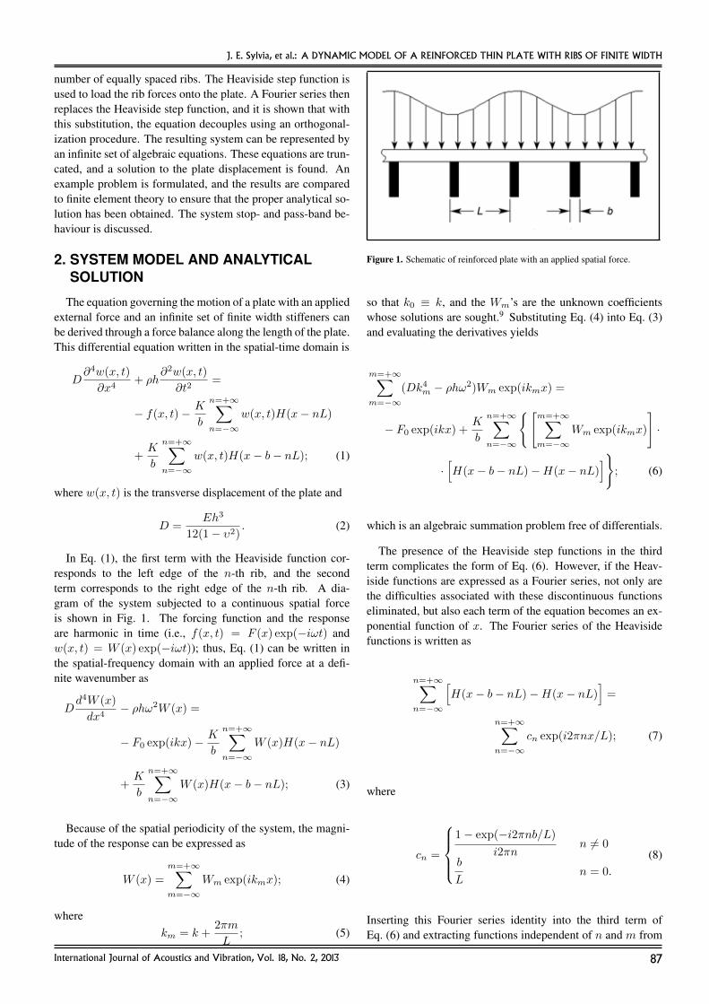
J. E. Sylvia, et al.: A DYNAMIC MODEL OF A REINFORCED THIN PLATE WITH RIBS OF FINITE WIDTH
number of equally spaced ribs. The Heaviside step function isused to load the rib forces onto the plate. A Fourier series thenreplaces the Heaviside step function, and it is shown that withthis substitution, the equation decouples using an orthogonal-ization procedure. The resulting system can be represented byan infinite set of algebraic equations. These equations are trun-cated, and a solution to the plate displacement is found. Anexample problem is formulated, and the results are comparedto finite element theory to ensure that the proper analytical so-lution has been obtained. The system stop- and pass-band be-haviour is discussed.
2. SYSTEM MODEL AND ANALYTICALSOLUTION
The equation governing the motion of a plate with an appliedexternal force and an infinite set of finite width stiffeners canbe derived through a force balance along the length of the plate.This differential equation written in the spatial-time domain is
D∂4w(x, t)
∂x4+ ρh
∂2w(x, t)
∂t2=
− f(x, t)− K
b
n=+∞∑n=−∞
w(x, t)H(x− nL)
+K
b
n=+∞∑n=−∞
w(x, t)H(x− b− nL); (1)
where w(x, t) is the transverse displacement of the plate and
D =Eh3
12(1− υ2). (2)
In Eq. (1), the first term with the Heaviside function cor-responds to the left edge of the n-th rib, and the secondterm corresponds to the right edge of the n-th rib. A dia-gram of the system subjected to a continuous spatial forceis shown in Fig. 1. The forcing function and the responseare harmonic in time (i.e., f(x, t) = F (x) exp(−iωt) andw(x, t) = W (x) exp(−iωt)); thus, Eq. (1) can be written inthe spatial-frequency domain with an applied force at a defi-nite wavenumber as
Dd4W (x)
dx4− ρhω2W (x) =
− F0 exp(ikx)−K
b
n=+∞∑n=−∞
W (x)H(x− nL)
+K
b
n=+∞∑n=−∞
W (x)H(x− b− nL); (3)
Because of the spatial periodicity of the system, the magni-tude of the response can be expressed as
W (x) =
m=+∞∑m=−∞
Wm exp(ikmx); (4)
wherekm = k +
2πm
L; (5)
Figure 1. Schematic of reinforced plate with an applied spatial force.
so that k0 ≡ k, and the Wm’s are the unknown coefficientswhose solutions are sought.9 Substituting Eq. (4) into Eq. (3)and evaluating the derivatives yields
m=+∞∑m=−∞
(Dk4m − ρhω2)Wm exp(ikmx) =
− F0 exp(ikx) +K
b
n=+∞∑n=−∞
{[m=+∞∑m=−∞
Wm exp(ikmx)
]·
·[H(x− b− nL)−H(x− nL)
]}; (6)
which is an algebraic summation problem free of differentials.
The presence of the Heaviside step functions in the thirdterm complicates the form of Eq. (6). However, if the Heav-iside functions are expressed as a Fourier series, not only arethe difficulties associated with these discontinuous functionseliminated, but also each term of the equation becomes an ex-ponential function of x. The Fourier series of the Heavisidefunctions is written as
n=+∞∑n=−∞
[H(x− b− nL)−H(x− nL)
]=
n=+∞∑n=−∞
cn exp(i2πnx/L); (7)
where
cn =
1− exp(−i2πnb/L)
i2πnn 6= 0
b
Ln = 0.
(8)
Inserting this Fourier series identity into the third term ofEq. (6) and extracting functions independent of n and m from
International Journal of Acoustics and Vibration, Vol. 18, No. 2, 2013 87
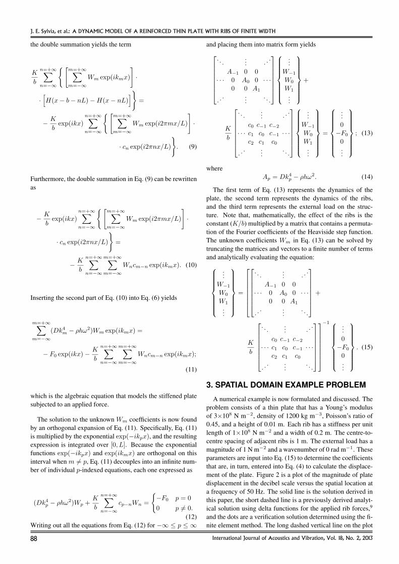
J. E. Sylvia, et al.: A DYNAMIC MODEL OF A REINFORCED THIN PLATE WITH RIBS OF FINITE WIDTH
the double summation yields the term
K
b
n=+∞∑n=−∞
{[m=+∞∑m=−∞
Wm exp(ikmx)
]·
·[H(x− b− nL)−H(x− nL)
]}=
− K
bexp(ikx)
n=+∞∑n=−∞
{[m=+∞∑m=−∞
Wm exp(i2πmx/L)
]·
· cn exp(i2πnx/L)
}. (9)
Furthermore, the double summation in Eq. (9) can be rewrittenas
− K
bexp(ikx)
n=+∞∑n=−∞
{[m=+∞∑m=−∞
Wm exp(i2πmx/L)
]·
· cn exp(i2πnx/L)
}=
− K
b
n=+∞∑n=−∞
m=+∞∑m=−∞
Wncm−n exp(ikmx). (10)
Inserting the second part of Eq. (10) into Eq. (6) yields
m=+∞∑m=−∞
(Dk4m − ρhω2)Wm exp(ikmx) =
− F0 exp(ikx)−K
b
n=+∞∑n=−∞
m=+∞∑m=−∞
Wncm−n exp(ikmx);
(11)
which is the algebraic equation that models the stiffened platesubjected to an applied force.
The solution to the unknown Wm coefficients is now foundby an orthogonal expansion of Eq. (11). Specifically, Eq. (11)is multiplied by the exponential exp(−ikpx), and the resultingexpression is integrated over [0, L]. Because the exponentialfunctions exp(−ikpx) and exp(ikmx) are orthogonal on thisinterval when m 6= p, Eq. (11) decouples into an infinite num-ber of individual p-indexed equations, each one expressed as
(Dk4p − ρhω2)Wp +K
b
n=+∞∑n=−∞
cp−nWn =
{−F0 p = 0
0 p 6= 0.
(12)Writing out all the equations from Eq. (12) for −∞ ≤ p ≤ ∞
and placing them into matrix form yields
. . .... . .
.
A−1 0 0
· · · 0 A0 0 · · ·0 0 A1
. .. ...
. . .
...
W−1W0
W1
...
+
K
b
. . .... . .
.
c0 c−1 c−2· · · c1 c0 c−1 · · ·
c2 c1 c0
. .. ...
. . .
...
W−1W0
W1
...
=
...
0
−F0
0...
; (13)
whereAp = Dk4p − ρhω2. (14)
The first term of Eq. (13) represents the dynamics of theplate, the second term represents the dynamics of the ribs,and the third term represents the external load on the struc-ture. Note that, mathematically, the effect of the ribs is theconstant (K/b) multiplied by a matrix that contains a permuta-tion of the Fourier coefficients of the Heaviside step function.The unknown coefficients Wm in Eq. (13) can be solved bytruncating the matrices and vectors to a finite number of termsand analytically evaluating the equation:
...
W−1W0
W1
...
=
. . .... . .
.
A−1 0 0
· · · 0 A0 0 · · ·0 0 A1
. .. ...
. . .
+
K
b
. . .... . .
.
c0 c−1 c−2· · · c1 c0 c−1 · · ·
c2 c1 c0
. .. ...
. . .
−1
...
0
−F0
0...
. (15)
3. SPATIAL DOMAIN EXAMPLE PROBLEM
A numerical example is now formulated and discussed. Theproblem consists of a thin plate that has a Young’s modulusof 3×10⁸ N m−2, density of 1200 kg m−3, Poisson’s ratio of0.45, and a height of 0.01 m. Each rib has a stiffness per unitlength of 1×10⁸ N m−2 and a width of 0.2 m. The centre-to-centre spacing of adjacent ribs is 1 m. The external load has amagnitude of 1 N m−2 and a wavenumber of 0 rad m−1. Theseparameters are input into Eq. (15) to determine the coefficientsthat are, in turn, entered into Eq. (4) to calculate the displace-ment of the plate. Figure 2 is a plot of the magnitude of platedisplacement in the decibel scale versus the spatial location ata frequency of 50 Hz. The solid line is the solution derived inthis paper, the short dashed line is a previously derived analyt-ical solution using delta functions for the applied rib forces,9
and the dots are a verification solution determined using the fi-nite element method. The long dashed vertical line on the plot
88 International Journal of Acoustics and Vibration, Vol. 18, No. 2, 2013

J. E. Sylvia, et al.: A DYNAMIC MODEL OF A REINFORCED THIN PLATE WITH RIBS OF FINITE WIDTH
Figure 2. Magnitude of plate displacement versus spatial location. The solidline is the analytical solution developed above, the short dashed line is theanalytical solution derived using a delta function for the application of the ribforces, and the dots are the finite element solution. The long dashed verticalline is the location of the right edge of the n = 0 rib.
indicates the spatial position of the right edge of the rib thatcorresponds to n = 0 in Eq. (1). This specific problem con-verged using 31 terms (−15 ≤ p ≤ 15), although it is notedthat convergence is a function of the specific parameters usedin the model.
The finite element model was created and analysed us-ing Abaqus FEA. The plate was modelled using 10000 solidquadrilateral two-dimensional plain strain elements, 1000 inthe longitudinal direction, and 10 in the transverse direction.The rib was modelled using 201 one-dimensional (vertical)translational spring elements equally distributed in the hori-zontal direction between x = 0 and x = b. A nodal tie con-straint was set up between the left and right edges of the plateto ensure periodic behaviour. The model was run using thesteady state dynamics solver. The analytical model and the fi-nite element model yield almost exactly the same results. Thisis because they both model the same structure and have the dy-namic components and enough degrees of freedom to properlycapture all of the dynamics present in the system, although wenote that these are two very different analysis techniques.
Several features in Fig. 2 are now noted. First, the plate/ribsystem is softer between the ribs and thus has a greater dis-placement at these spatial locations. As a result, if the stiffnessof the ribs approaches zero, the solution approaches that of anunreinforced plate. Second, even though the ribs are fairly stiffin this example, they still exhibit dynamic behaviour acrosstheir spatial extent. As evidence, examine Fig. 2 in the areafrom x = 0 to x = b = 0.2 m. Each rib has almost 40 dBof motion in this relatively small space, although the displace-ment is significantly lower than the plate displacement betweenthe ribs. Third, although not explicitly shown in Fig. 2, the so-lution is periodic on x ∈ [0, L]. Sectional aperidocity can beadded to the model using previously developed techniques.5
Fourth, it is noted that when the width of the ribs approacheszero, the solution derived above (solid line) will approach thesolution derived using delta functions for the applied rib forces(short dashed line).
Figure 3. Dispersion curve for b = 0.01 m. The solid line is the free wavepropagation locations, the grey areas are the system stop bands, and the dashedline is the dispersion curve of the plate only.
4. STOP- AND PASS-BAND BEHAVIOUR
The stop- and pass-band behaviour of this system can beexamined by calculating when the determinant of the systemmatrix is zero with respect to frequency and wavenumber vari-ation. Specifically, when
det
. . .... . .
.
A−1 0 0
· · · 0 A0 0 · · ·0 0 A1
. .. ...
. . .
+
K
b
. . .... . .
.
c0 c−1 c−2· · · c1 c0 c−1 · · ·
c2 c1 c0
. .. ...
. . .
= 0; (16)
free wave propagation can exist. Figures 3 and 4 are plots ofthe free wave propagation (dispersion) curves generated fromEq. (16) when b = 0.01 m and b = 0.02 m, respectively.In these figures, the x-axis is wavenumber, the y-axis is fre-quency, the solid lines are the locations of free wave propaga-tion, the grey areas are stop-bands, and the dashed line is thesystem dispersion curve when K = 0 (no ribs). Figure 5 is aplot of the ratio of rib width to rib spacing versus the percentpass-band analysed from 0 to 200 Hz. This analysis allows thesystem pass-band behaviour to be characterized as a functionof rib width.
5. CONCLUSIONS
A model of a reinforced thin plate with ribs of finite thick-ness was derived, and the solution was obtained using an or-thogonalization procedure. It was shown that the effect of theribs is mathematically a constant multiplied by a matrix that
International Journal of Acoustics and Vibration, Vol. 18, No. 2, 2013 89

J. E. Sylvia, et al.: A DYNAMIC MODEL OF A REINFORCED THIN PLATE WITH RIBS OF FINITE WIDTH
Figure 4. Dispersion curve for b = 0.02 m. The solid line is the free wavepropagation locations, the grey areas are the system stop bands, and the dashedline is the dispersion curve of the plate only.
contains a permutation of the Fourier coefficients of the Heav-iside step function. A numerical example was presented andcompared to a finite element analysis and a previous solutionto a related problem. This new analytical solution was in al-most exact agreement with the finite element solution. Thestop- and pass-band behaviour of the model with respect to ribwidth is characterized.
ACKNOWLEDGEMENTS
This paper was funded by the Naval Undersea WarfareCenter’s In-House Laboratory Independent Research Program,Program Manager Dr. Anthony A. Ruffa. Jaclyn E. Sylvia wasfunded by the Office of Naval Research Naval Research Enter-prise Intern Program.
REFERENCES1 Mace, B. R. Periodically stiffened fluid-loaded plates, I: Re-
sponse to convected harmonic pressure and free wave prop-agation, J. Sound Vib., 73 (4), 473–486, (1980).
2 Mace, B. R. Periodically stiffened fluid-loaded plates, II:Response to line and point forces, J. Sound Vib., 73 (4),487–504, (1980).
Figure 5. Ratio of rib width to rib spacing versus percent pass band from 0 to200 Hz.
3 Stepanishen, P. R. The acoustic transmission and scatteringcharacteristics of a plate with line impedance discontinu-ities, J. Sound Vib., 58 (2), 257–272, (1978).
4 Eatwell, G. P. and Butler D. The response of a fluid-loaded, beam-stiffened plate, J. Sound Vib., 84 (3), 371–388, (1982).
5 Cray, B. A. Acoustic radiation from periodic and sec-tionally aperiodic rib-stiffened plates, J. Acoust. Soc. Am.,95 (1), 256–264, (1994).
6 Hull, A. J. Elastic response of an acoustic coating on a rib-stiffened plate, J. Sound Vib., 329 (20), 4192–4211, (2010).
7 Woolley, B. L. Acoustic scattering from a submerged plate.I. One reinforcing rib, J. Acoust. Soc. Am., 67 (5), 1642–1653, (1980).
8 Woolley, B. L. Acoustic scattering from a submerged plate.II. Finite number of reinforcing ribs, J. Acoust. Soc. Am.,67 (5), 1654–1658, (1980).
9 Mead, D. J. and Pujara, K. K. Space-harmonic analysis ofperiodically supported beams: Response to convected ran-dom loading, J. Sound Vib., 14 (4), 525–541, (1971).
90 International Journal of Acoustics and Vibration, Vol. 18, No. 2, 2013

A Simplified Formula for Calculating the SoundPower Radiated by Planar StructuresYu DuSchool of Automotive Engineering, State Key Laboratory of Structural Analysis for Industrial Equipment, DalianUniversity of Technology, Dalian 116024, ChinaState Key Laboratory of Vehicle NVH and Safety Technology, Chongqing 401120, China
Jun ZhangState Key Laboratory of Vehicle NVH and Safety Technology, Chongqing 401120, ChinaChangan Automobile Engineering Institute, NVH Department, Chongqing 401120, China
(Received 23 May 2012; Revised 13 February 2013; Accepted 21 February 2013)
Based on the wave number transform, the sound power radiated by a planar structure embedded in a baffle canbe derived theoretically as a double integral within the range of supersonic wave numbers. Due to the specificform of the integrand, a singularity problem is encountered at the integration boundary that leads to difficultiesin evaluating the sound power directly. This technical note discusses a mathematical method for simplifying theoriginal formula to avoid this singularity problem by using a technique of substituting variables. Compared toits original counterpart, the simplified formula not only eliminates the singularity points but also converges muchmore rapidly when evaluating the double integrals numerically.
1. INTRODUCTION
In noise control engineering, the sound power generated bya structure often needs to be evaluated analytically for designand/or troubleshooting purposes. A classical model that istypically used in practice to describe the sound radiation be-haviour of planar structures consists of a plate embedded inan infinite baffle. In the frequency domain, the sound powerradiated by this finite plate is normally expressed as a two-dimensional integral within a finite area as shown below:1
W (ω) =ωρ
8π2
x
k>√k2x+k
2y
|V (kx, ky)|2√k2 − (k2x + k2y)
dkxdky; (1)
where W is the sound power, ω is the radian frequency, ρ isthe ambient medium density, k is the acoustic wave number ofthe ambient medium that is given as k = ω/c; c is the speedof sound in the medium, kx and ky are x and y componentsof the flexural wave number of the plate, and V (kx, ky) is thetwo-dimensional velocity wave number transform of the plate,which can be expressed as
V (kx, ky) =
∫ ∞x=−∞
∫ ∞y=−∞
v(x, y)eikxxeikyydxdy; (2)
in which v(x, y) is the velocity distribution on the plate andi =√−1 is the unit imaginary number.
Based on the acoustical theory, only the supersonic wavenumber components contribute to the sound power radiation.2
Thus, the original formula in Eq. (1) requires that the integral iscalculated within the range in which the flexural wave numberof the structure (
√k2x + k2y) is less than the acoustical wave
number (k) in the ambient medium. This requirement inducesa singularity problem in the integral when the denominator ofthe integrand is zero at the boundary of k =
√k2x + k2y . There-
fore, to obtain reliable results, we must handle this singularityproblem carefully when evaluating the sound power directly inaccordance to Eq. (1). One possible way to avoid the singular-ity is letting the integration range infinitesimally approach butnever reach the boundary. That is, the original integration canbe approximated as
W (ω) =ωρ
8π2
∫ ky=σk
ky=−σk
∫ kx=σky
kx=−σky
|V (kx, ky)|2√k2 − (k2x + k2y)
dkxdky;
(3)where σ is a weighting coefficient whose value is between 0and 1. Although Eq. (3) does not suffer from the singularityproblem, it inevitably introduces a truncation error in the dou-ble integral since the weighting coefficient σ can never be 1.Obviously, the closer the value of σ to 1, the more accurate theresult will be.
Although other approaches such as the elemental-radiatormethod3, 4 may also be considered to estimate the sound power,the current study focuses on a mathematical method for sim-plifying the original formula so that the singularity problemis removed without introducing the above-mentioned trunca-tion error. The advantages of the simplified formula are alsodemonstrated by comparing the convergence rates of the twomethods using a numerical example.
International Journal of Acoustics and Vibration, Vol. 18, No. 2, 2013 (pp. 91–93) 91
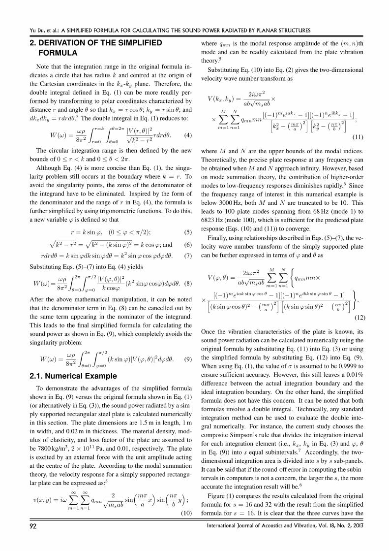
Yu Du, et al.: A SIMPLIFIED FORMULA FOR CALCULATING THE SOUND POWER RADIATED BY PLANAR STRUCTURES
2. DERIVATION OF THE SIMPLIFIEDFORMULA
Note that the integration range in the original formula in-dicates a circle that has radius k and centred at the origin ofthe Cartesian coordinates in the kx-ky plane. Therefore, thedouble integral defined in Eq. (1) can be more readily per-formed by transforming to polar coordinates characterized bydistance r and angle θ so that kx = r cos θ; ky = r sin θ; anddkxdky = rdrdθ.3 The double integral in Eq. (1) reduces to:
W (ω) =ωρ
8π2
∫ r=k
r=0
∫ θ=2π
θ=0
|V (r, θ)|2√k2 − r2
rdrdθ. (4)
The circular integration range is then defined by the newbounds of 0 ≤ r < k and 0 ≤ θ < 2π.
Although Eq. (4) is more concise than Eq. (1), the singu-larity problem still occurs at the boundary where k = r. Toavoid the singularity points, the zeros of the denominator ofthe integrand have to be eliminated. Inspired by the form ofthe denominator and the range of r in Eq. (4), the formula isfurther simplified by using trigonometric functions. To do this,a new variable ϕ is defined so that
r = k sinϕ, (0 ≤ ϕ < π/2); (5)√k2 − r2 =
√k2 − (k sinϕ)2 = k cosϕ; and (6)
rdrdθ = k sinϕdk sinϕdθ = k2 sinϕ cosϕdϕdθ. (7)
Substituting Eqs. (5)–(7) into Eq. (4) yields
W (ω)=ωρ
8π2
∫ 2π
θ=0
∫ π/2
ϕ=0
|V (ϕ, θ)|2
k cosϕ(k2 sinϕ cosϕ)dϕdθ. (8)
After the above mathematical manipulation, it can be notedthat the denominator term in Eq. (8) can be cancelled out bythe same term appearing in the nominator of the integrand.This leads to the final simplified formula for calculating thesound power as shown in Eq. (9), which completely avoids thesingularity problem:
W (ω) =ωρ
8π2
∫ 2π
θ=0
∫ π/2
ϕ=0
(k sinϕ)|V (ϕ, θ)|2dϕdθ. (9)
2.1. Numerical ExampleTo demonstrate the advantages of the simplified formula
shown in Eq. (9) versus the original formula shown in Eq. (1)(or alternatively in Eq. (3)), the sound power radiated by a sim-ply supported rectangular steel plate is calculated numericallyin this section. The plate dimensions are 1.5 m in length, 1 min width, and 0.02 m in thickness. The material density, mod-ulus of elasticity, and loss factor of the plate are assumed tobe 7800 kg/m3, 2 × 10¹¹ Pa, and 0.01, respectively. The plateis excited by an external force with the unit amplitude actingat the centre of the plate. According to the modal summationtheory, the velocity response for a simply supported rectangu-lar plate can be expressed as:5
v(x, y) = iω∞∑m=1
∞∑n=1
qmn2√msab
sin(mπax)sin(nπby);
(10)
where qmn is the modal response amplitude of the (m,n)thmode and can be readily calculated from the plate vibrationtheory.5
Substituting Eq. (10) into Eq. (2) gives the two-dimensionalvelocity wave number transform as
V (kx, ky) =2iωπ2
ab√msab
×
×M∑m=1
N∑n=1
qmnmn[(−1)meiakx − 1][(−1)neibky − 1][
k2x −(mπa
)2] [k2y −
(nπb
)2] ;
(11)
where M and N are the upper bounds of the modal indices.Theoretically, the precise plate response at any frequency canbe obtained whenM andN approach infinity. However, basedon mode summation theory, the contribution of higher-ordermodes to low-frequency responses diminishes rapidly.6 Sincethe frequency range of interest in this numerical example isbelow 3000 Hz, both M and N are truncated to be 10. Thisleads to 100 plate modes spanning from 68 Hz (mode 1) to6823 Hz (mode 100), which is sufficient for the predicted plateresponse (Eqs. (10) and (11)) to converge.
Finally, using relationships described in Eqs. (5)–(7), the ve-locity wave number transform of the simply supported platecan be further expressed in terms of ϕ and θ as
V (ϕ, θ) =2iωπ2
ab√msab
M∑m=1
N∑n=1
{qmnmn×
× [(−1)meiak sinϕ cos θ − 1][(−1)neibk sinϕ sin θ − 1][(k sinϕ cos θ)2 −
(mπa
)2] [(k sinϕ sin θ)2 −
(nπb
)2]}.
(12)
Once the vibration characteristics of the plate is known, itssound power radiation can be calculated numerically using theoriginal formula by substituting Eq. (11) into Eq. (3) or usingthe simplified formula by substituting Eq. (12) into Eq. (9).When using Eq. (1), the value of σ is assumed to be 0.9999 toensure sufficient accuracy. However, this still leaves a 0.01%difference between the actual integration boundary and theideal integration boundary. On the other hand, the simplifiedformula does not have this concern. It can be noted that bothformulas involve a double integral. Technically, any standardintegration method can be used to evaluate the double inte-gral numerically. For instance, the current study chooses thecomposite Simpson’s rule that divides the integration intervalfor each integration element (i.e., kx, ky in Eq. (3) and ϕ, θin Eq. (9)) into s equal subintervals.7 Accordingly, the two-dimensional integration area is divided into s by s sub-panels.It can be said that if the round-off error in computing the subin-tervals in computers is not a concern, the larger the s, the moreaccurate the integration result will be.6
Figure (1) compares the results calculated from the originalformula for s = 16 and 32 with the result from the simplifiedformula for s = 16. It is clear that the three curves have the
92 International Journal of Acoustics and Vibration, Vol. 18, No. 2, 2013

Yu Du, et al.: A SIMPLIFIED FORMULA FOR CALCULATING THE SOUND POWER RADIATED BY PLANAR STRUCTURES
Figure 1. Calculated sound power of a simply supported steel plate with di-mensions of 1.5 by 1 by 0.02 m excited by a unit force at its geometrical center.The variable s indicates the number of the integration subinterval.
same shape and agree very well at most frequencies. How-ever, at some frequencies, the discrepancy between the resultsobtained from the original and the simplified formulas couldbe as high as 10 dB. Figure (1) also shows that as s increases,the prediction from the original formula approaches that fromthe simplified formula calculated with a lower s value. Thiscan be further demonstrated in Fig. (2) that examines the in-tegration convergence rates as a function of s. For exam-ple, the sound power at 1000 Hz evaluated using the originaland the simplified methods are compared as s increases. Ob-serve that the simplified method converges to a stable valueof 2.002 × 10⁻⁷ after s = 16, while the original methodcontinuously approaches this value with increasing s. Whens = 200, the best result obtained from the original method is2.048 × 10−7, giving a 2.3% error compared to the value ob-tained by the simplified method at s = 16. This result clearlyshows that the simplified method is much more efficient thanthe original method in computing the sound power.
3. CONCLUSIONS
When using the direct formula shown in Eq. (1) to calculatethe sound power radiated by a planar structure embedded ina baffle, a singularity problem is always encountered becausethe denominator of the integrand has zeros at the integrationboundary. This study presents a new technique to simplifythe original formula so as to eliminate the singularity problem.Moreover, the simplified formula also leads to more accurateresults at a computational cost much less than that required bythe original formula.
ACKNOWLEDGEMENTS
This work was funded by the National Basic ResearchProject (973 Project) of China (No. 2010CB736104) and theState Key Laboratory of Vehicle NVH and Safety Technology(No. NVHSKL-201111). The authors gratefully acknowledgethe financial support from these funding sources.
Figure 2. Convergence trend of the calculated sound power at 1000 Hz as thenumber of the integration subinterval s increases.
Bibliography1 Cremer, L., Heckl, M., and Ungar, E. E. Structure-borne
sound, Springer-Verlag, Berlin, (1987).
2 Fahy, F. Sound and structural vibration – Radiation, trans-mission and response, Academic Press, London, (1985).
3 Elliott, S. J. and Jonson, M. E. Radiated modes and the ac-tive control of sound power, Journal of the Acoustical Soci-ety of America, 94 (4), 2194–2204, (1993).
4 Du, Y., Burdisso, R., and Efstratios, N. Control of internalresonances in isolation isolators using passive and hybriddynamic vibration absorbers, Journal of Sound and Vibra-tion, 286 (4–5), 697–727, (2005).
5 Meirovitch, L. Principles and techniques of vibrations,Prentice Hall, (1997).
6 Du, Y. and Zhang, J. Structural-acoustic coupling charac-teristics of a rectangular enclosure with lightweight designconsiderations, Noise Control Engineering Journal, 60 (6),726–739, (2012).
7 Davis, P. J. and Rabinowits, P. Methods of numerical inte-gration, Academic Press, Orlando, Florida, (1984).
International Journal of Acoustics and Vibration, Vol. 18, No. 2, 2013 93

About the Authors
Dishan Huang was born in Shaoxing, China, in 1957 and obtained a PhD from the Depart-ment of Mechanical Engineering at Zhejiang University. Now he teaches courses on vibrationand mechanical design and carries out research as an associate professor at Shanghai Univer-sity. His current research focuses on response approach and stability of parametric vibrationand wave propagation in rotating bodies with applications to structure design and advancedmanufacturing.
Chenchen Fu was born in Shanghai in 1989 and is a graduate student in the Department ofMechanical Engineering at Shanghai University, China. His research focuses on responseapproach of parametric vibration and parametric vibration testing and control in mechanicalsystems.
S. N. Panigrahi obtained a masters degree and PhD from Indian Institute of Science, Ban-galore, India, in the year 2007. His doctoral work dealt with analysis of multiply-connectedacoustical filters with application to design of underwater noise control linings. After work-ing for two years in the field of industrial computational mechanics, he moved to IndianInstitute of Technology Bhubaneswar, India, where he has been working as a faculty membersince July 2009. His present research interests lie in technical acoustics, automotive noisecontrol, acoustics and vibration signal processing, musical acoustics, and underwater soundabsorbers.
Dibya Prakash Jena obtained a masters degree from BITS Pilani, India, and joined IndianInstitute of Technology Bhubaneswar, India, as a research scholar in the School of Mechani-cal Sciences. He is presently pursuing a doctoral degree in the area of vibration and acousticalemission-based condition monitoring and the effect of active and passive filters thereon. Heis on sabbatical from Robert Bosch, Bangalore, India, where he has been working since Oc-tober 2008. His interests lie in industrial automation, automotive cluster, and high-speed dataacquisition in which he has acquired expertise while working with John Deere TechnologyCentre, Pune and Captronics Systems, Bangalore before joining his present company.
94 International Journal of Acoustics and Vibration, Vol. 18, No. 2, 2013

About the AuthorsM. L. Munjal has been on the faculty of Indian Institute of Science since 1968. He haspublished over 185 papers in professional journals. He has authored a book Acoustics ofDucts and Mufflers (WileyInterscience, New York, 1987) and chapters in handbooks. He hasexecuted nearly 100 industrial consultancy projects on different aspects of noise control andquieter designs, with particular application to automobiles. Prof. Munjal has been convenerof the Facility for Research in Technical Acoustics since its inception in 1998. Since 1988, hehas been a Distinguished International Member of the Institute of Noise Control Engineeringof USA. Recently, Prof. Munjal has been elected as Honorary Fellow of the InternationalInstitute of Acoustics and Vibration. Currently, he is a member of the editorial board of theInternational Journal of Acoustics and Vibration.
Jaclyn E. Sylvia received two BA degrees in mathematics and English from College of theHoly Cross, Worcester, Massachusetts, USA, in 2010. She previously worked as an Office ofNaval Research Intern in the Autonomous Systems and Technology Department at the NavalUndersea Warfare Center in Newport, Rhode Island, USA. She is currently teaching Englishin Korea.
Andrew J. Hull received a BS degree in 1983, MS degree in 1985, and PhD degree in 1990,all in mechanical engineering from Michigan State University, East Lansing, Michigan, USA.He currently works as a mechanical engineer in the Autonomous Systems and TechnologyDepartment at the Naval Undersea Warfare Center in Newport, Rhode Island, USA. His re-search interests are in the areas of mechanical vibrations, acoustics, and boundary value prob-lems. He is a member of the International Institute of Acoustics and Vibrations and a fellowof the Acoustical Society of America.
Yu Du received a BS and MS in vehicle engineering from Tsinghua University (Beijing,China) in 1997 and 1999 respectively and a PhD in mechanical engineering from VirginiaTech (Blacksburg, Virginia, USA) in 2003. He was a research scientist at Adaptive Tech-nologies, Inc. (Blacksburg, Virginia, USA) from 2003 to 2009, then at Knowles Electronics,LLC (Itasca, Illinois, USA) from 2009 to 2010. He is currently a professor at the School ofAutomotive Engineering in Dalian University of Technology (Dalian, China). His researchinterests include passive and active control of sound and vibration, vehicle NVH, noise andvibration of lightweight structures, and acoustical signal processing.
Jun Zhang received a PhD in mechanical engineering from Shanghai Jiaotong University(Shanghai, China) in 2006. He has been working at Chongqing Changan Auto R&D Center,Inc. (Chongqing, China) since his graduation and is currently a staffengineer at the NVHResearch Instituteof Changan Auto R&D Center, Inc. His current research interests are NVHanalysis and mitigation in transportation engineering, such as automobile, launchvehicles,and ship structures.
International Journal of Acoustics and Vibration, Vol. 18, No. 2, 2013 95

Book ReviewsDynamic Methods for DamageDetection in Structures: CISM Coursesand Lectures, vol. 499
Edited by: Antonino Morassi and Fabrizio VestroniSpringer, Wien, New York, 2008, 221 p., 108 illus.ISBN: 978-3-211-78776-21Price: US $139
This book is written for researcherswho are interested in advanced lec-tures in dynamic methods for damagedetection. The first chapter outlinesthe dynamic characterization of dis-crete systems.
Chapter 2 provides an overview ofinverse methods in damage identifica-tion and discusses difficulties in in-verse methods in detail. The simu-lated examples presented in this chap-ter help the readers understand thedifficulties, including regularisationtechniques, parametric models of damage, and sensor valida-tion.
Chapter 3 proposes a method to estimate the physical pa-rameters of structures using dynamic response measurements.A numerical example shows that the predicted physical param-eters do not vary with the locations of the dynamic measure-ments. The possibility to assess structural damage by compar-ing the undamaged and damaged estimates is briefly discussed.
Chapter 4 reviews structural identification techniques basedon parametric models. A procedure for identifying the lin-ear finite element model is described. The effects of elementmesh size on the frequency response function prediction arediscussed with a lattice structure study.
Chapter 5 continues the use of parametric models to differ-ent damage identifications. The first part examines the abilityto estimate local characteristics of structures affected by dif-fused damage with an experimental investigation on a masonrybuilding. The second part proposes a procedure for identifica-tion of concentrated damage.
Chapter 6 provides a comprehensive overview of inversemethods for damage detection in vibrating beams. Differentcases are presented, including longitudinal and bending vibra-tion, general damage, and open crack identification. Besidesnatural frequency measurements, techniques that make use ofchanges in anti-resonances and in nodes of mode shapes arediscussed.
Chapter 7 describes a simple approach to damage localiza-tion based on frequency changes introduced by damage. Asimple crack locator model is implemented to locate crackswith closure.
Chapter 8 presents a detailed study of the reflection of thefundamental torsional mode from defects in pipelines. The ex-perimental setup and finite element model are described. Thesensitivity of the finite element model is examined. A compar-ison between the measured and predicted coefficients is pre-sented.
Chapter 9 introduces the use of auxiliary systems to enhancethe sensitivity of the frequency response to local variations ofmechanical characteristics. A case of a beam-like structurecoupled to piezoelectric patches is briefly discussed.
This book focuses on inverse methods for damage detectionin structures. The reader can obtain a satisfactory review of
inverse methods from the first two chapters. The rest of thebook, chapters 3 to 8, presents updated advanced techniquesfor detecting damage with discussions of real-life applications.Overall, this is a good book on dynamic methods for damagedetection in structures.
Ran ZhouScore Atlanta Inc., Kennesaw, Georgia, USA
Vibrations of Mechanical Systems withRegular Structure
By Liudmila Ya. Banakh and Mark L KempnerSpringer, 2010, XII, 252 p.ISBN: 978-3-642-03126-7Price: US $ 209
This book is in two parts. Part I,written by the first author, looks at vi-brations systems with lumped param-eters, while Part II, written by the sec-ond author, studies systems with dis-tributed parameters. A third author, P.S. Akhmetkhanov, wrote a section inPart I on dynamic properties of lam-inar systems. The work is based onoriginal research by the authors.
Regular structures are defined asperiodic structures consisting of re-peated elements, as well as structureswith repeated symmetry. The book contents are quite con-densed, but give a good account of methods using lumpedparameter models and the use of idealized elements with dis-tributed parameters and known analytical solutions. In Part I,a fresh approach to using finite element methods is adopted.FEM being usually used as a tool for numerical calculations,the author of this section draws attention to the fact that it hascapabilities for obtaining interesting analytical results, makinguse of FEM matrices for analytical solutions. Regular systemsof periodic structure are considered using a wave approach andmodels using superposition of wave motions are described.Frames with periodic structure are considered by combiningfinite element methods and dispersion equations, as are beamsystems. Quasi-symmetrical systems are considered includingvibroisolation, and an example is given of a dynamic model ofplanetary reduction gear.
Part II begins with basic equations and numerical methods,and then deals with systems of periodic structure and systemswith cyclic symmetry, systems with reflection symmetry ele-ments and self-similar structures. Vibrations of rotor systemswith periodic structures are considered as regular ribbed cylin-drical cells. Fractals, in which every consecutive element isformed from the preceding one by scaling before being addedto regular structures, are described.
The book contains many numerical examples of real-life en-gineering structures, in particular aviation engines. There is auseful list of 115 references (over 20 by the book’s authors)and four appendices describing stiffness and inertia matrices.
This book is an important addition to the library, being morethan just a résumé of known mathematical techniques with theaddition of an explanation of the authors’ original work.
Rupert Thornely-TaylorRuper Taylor Ltd., UK
96 International Journal of Acoustics and Vibration, Vol. 18, No. 2, 2013