International Cost of Capital - Understanding and

INTERNATIONAL COST OF CAPITAL: UNDERSTANDING AND QUANTIFYING COUNTRY RISK

03

2903 — International Cost of Capital: Understanding and Quantifying Country Risk

INTERNATIONAL COST OF CAPITAL: UNDERSTANDING AND QUANTIFYING COUNTRY RISK1 James Harrington and Carla Nunes

The cost of capital may be described in simple terms as the expected return appropriate for the expected level of

risk.2 The cost of capital is also commonly called the discount rate, the expected return, or the required return.3

A basic insight of capital market theory, that expected return is a function of risk, still holds when dealing with cost

of equity capital in a global environment.

“Practitioners typically are confronted with this situation: “I know how to value a company in the United

States, but this one is in Country X, a developing economy. What should I use for a discount rate?”4

Estimating an appropriate cost of capital (i.e., a discount rate) in developed countries, where a relative abundance

of market data and comparable companies exist, requires a high degree of expertise. Estimating cost of capital in

less-developed (i.e., “emerging”) countries can present an even greater challenge, primarily due to lack of data (or

poor data quality) and the potential for magnified financial, economic, and political risks.

“Measuring the impact of country risk is one of the most vexing issues in finance, particularly in emerging

markets, where political and other country-specific risks can significantly change the dynamics of the

project. It is absolutely essential to incorporate these risks into either the expected cash flows or the

discount rate. While this point is not controversial, the key is using a reliable method to quantify these extra

country risks.”5

This article provides an overview of international cost of capital issues.6

Are Country Risks Real?

Why should there be any incremental challenges when developing cost of capital estimates for a business,

business ownership interest, security, or intangible asset based outside the United States (or outside a mature,

developed country like Canada)?

1 This article is a summary of the June 21, 2019 presentation entitled “International Cost of Capital; Understanding and Quantifying

Country Risk” by James P. Harrington at the CBV Institute 2019 National Business Valuation Congress. Mr. Harrington a Director in

Duff & Phelps’ Business Publications Group, co-author of the Duff & Phelps “Valuation Handbook” series, and a co-creator of

Duff & Phelps online Cost of Capital Navigator platform. To learn more, visit dpcostofcapital.com. Thank you to Carla Nunes, Jamie

Warner, Anas Aboulamer, Kevin Madden, Aaron Russo and Kevin Latz of Duff & Phelps for their assistance in preparing this paper.

2 Modern portfolio theory and related asset pricing models assume that investors are risk-averse. This means that investors try to

maximize expected return for a given amount of risk, or minimize risk for a given amount of expected return.

3 When a business uses a given cost of capital to evaluate a commitment of capital to an investment or project, it often refers to that

cost of capital as the “hurdle rate”. The hurdle rate is the minimum expected rate of return that the business would be willing to

accept to justify making the investment.

4 Shannon P. Pratt and Roger J. Grabowski, Cost of Capital: Applications and Examples 5th ed. (Hoboken, NJ: John Wiley & Sons, 2014).

5 Campbell R. Harvey, Professor of Finance at the Fuqua School of Business, Duke University; Research Associate of the National

Bureau of Economic Research in Cambridge, Massachusetts; President of the American Finance Association in 2016

6 For a more detailed discussion, please see the Valuation Handbook – International Guide to Cost of Capital, accessible through the

Cost of Capital Navigator: International Cost of Capital Module. To learn more or to subscribe, visit: dpcostofcapital.com.

03 —International Cost of Capital: Understanding and Quantifying Country Risk30

If investors are alike everywhere and international capital markets are integrated (i.e., investors can easily and

freely transact in any country around the globe), then the task is relatively simple. However, if markets are (entirely

or partially) isolated (i.e., segmented) from world markets, then we need to address the perceived (and real) risk

differences between markets.

“Segmentation” in this context refers to markets (i.e., economies) that are not fully integrated into world markets

(i.e., are to some degree isolated from world markets). Markets may be segmented due to a host of issues, usually

categorized as “financial”, “economic”, or “political” risks. These risks can include: (i) regulation that restricts

foreign investment, (ii) taxation differences, (iii) legal factors, (iv) information deficiencies, (v) trading costs, (vi)

political instability, and (vii) physical barriers, among others. Experts do not agree on the extent or effects of

market segmentation, although there can be no doubt that some markets are at least partially segmented.

The most common adjustments made by practitioners aimed at this segmentation problem are addressed by

adding ad hoc country-specific risk premia (CRPs) to cost of capital estimates.

While in today’s increasingly integrated economy there may be less theoretical justification for country risk premia

than may have been warranted even a few decades ago, these risks still exist in the real world, and it would likely

be unwise to make investment decisions without considering these incremental risks.

A Common Error

A common error in estimating international cost of capital is mixing currencies. According to corporate finance

theory, the currency of the projections should always be consistent with the currency of the discount rate. In

practice, this means that the inputs used to derive a discount rate (the discount rate is included in the denominator

in a discounted cash flow (DCF) model) should be in the same currency used to project cash flows (the numerator

in a DCF model). For example, if cash flow projections are denominated in Canadian Dollars, then the risk-free rate,

equity risk premium, and other discount rate inputs should also be denominated in Canadian Dollar terms.

There are two basic methods to address foreign currency cash flows in valuations, assuming the analysis is being

conducted in nominal terms:

• Perform the valuation in the Investee Country7 currency, discount the projected cash flows with a discount

rate denominated in the Investee Country currency (i.e., developed using inputs denominated in the

Investee Country currency), and convert the resulting value conclusion into the Investor Country8 currency

(e.g., CAD, USD, EUR) at the spot exchange rate.

• Convert cash flows at a forecasted exchange rate into the Investor Country currency (e.g., CAD, USD,

EUR) and discount the projected cash flows with an Investor Country discount rate (i.e., developed using

inputs denominated in the Investor Country currency). In this case, the forecasted exchange rate already

includes the risk associated with exchange rate fluctuations.

What if Reliable Local Inputs are Not Available?

Notwithstanding the two general approaches outlined in the previous section, valuation and finance professionals

may find themselves in a position where a local currency discount rate is needed and yet there are no reliable cost

of capital inputs in the local (foreign) currency (i.e., the Investee Country currency). What should you do in such

a situation?

One can go back to one of the central ideas in international finance: the so-called “law of one price”.

7 The “Investee Country” is the country in which the investment is located. For example, if a Canadian investor is evaluating an

investment located in Germany, the Investee Country is Germany, and the “Investor Country” is Canada.

8 The term “Investor Country” is closely related to the concept of “investor perspective”. In the previous example, the German

investment is being evaluated from the “perspective” of a Canadian investor.


The basic idea is that international investors explore profit arbitrage opportunities across financial markets in

different countries, therefore guaranteeing that identical financial assets have similar prices, once adjusted for

different currencies. This presumes competitive markets, where market imperfections do not exist.

Five key theoretical economic relationships result from these arbitrage activities: (i) Purchasing Power Parity,

(ii) Fisher Effect, (iii) International Fisher Effect, (iv) Interest Rate Parity, and (v) Forward Rates as Unbiased

Predictors of Future Spot Rates9

It is beyond this article’s scope to discuss these concepts on a detailed level. Several international finance

textbooks have been written and published which cover this topic extensively. These theoretical relationships are

also central to understanding and forecasting foreign exchange rates, as well as prices of other financial assets

denominated in foreign currencies.10

The International Fisher Effect is formalized in Equation 1.

Equation 1: The International Fisher Effect Equation

(1 + Inflation )

(1 + Inflation )

Interest Rate

(1 + Interest Rate ) 1×

=

—Investor Country Currency

Investee Country CurrencyInvestee Country Currency

Investor Country Currency

The International Fisher Effect suggests that countries with high inflation rates should expect to see higher

interest rates relative to countries with lower inflation rates. This relationship can be extended from interest rates

into discount rates, thereby allowing us to translate a home (or Investor Country) currency cost of capital estimate

into a foreign (or Investee Country) currency indication.

However, it is crucial to understand that the International Fisher Effect relationship holds only in equilibrium.

This presumes that (i) there is no government intervention in capital markets; and (ii) capital can flow freely in

international financial markets from one currency to another, such that any potential arbitrage opportunity across

countries will be quickly eliminated. In reality, market frictions (e.g., transaction costs, regulations, etc.)

and government interventions do exist in practice, which means that using the International Fisher Effect to

translate the home currency discount rate into a local currency will result in only an approximation.

Despite these limitations, the International Fisher Effect can be useful in ensuring that inflation assumptions

embedded in the projected cash flows are consistent with those implied by discount rates.11

Applying the International Fisher Effect to translate rates of return on equity and debt would result in the

relationships expressed in Equation 2 and Equation 3, respectively.

Equation 2: International Fisher Effect Applied to Cost of Equity Capital

(1 + Inflation )

(1 + Inflation )

Cost of Equity Capital

(1 + Cost of the Equity Capital ) 1×

=

—Investor Country Currency

Investee Country Currency

Investor Country Currency


9 Alan C. Shapiro, Multinational Financial Management, 10th ed. (Hoboken, NJ: John Wiley & Sons, 2013).

10 See for example: i) Chapters 4 and 19 of Piet Sercu (2009), International Finance: Theory into Practice, (Princeton, NJ: Princeton

University Press); and ii) Chapter 4 of Alan C. Shapiro (2013), Multinational Financial Management, 10th ed. (Hoboken, NJ: John Wiley

& Sons, 2013).

11 For a discussion and examples of how to apply the methods outlined in this section, refer to the complimentary CFA Institute webinar

entitled “Quantifying Country Risk Premiums”, presented on December 6, 2016 by James P. Harrington and Carla S. Nunes, CFA, both

of Duff & Phelps. This webcast can be accessed here: https://www.cfainstitute.org/en/research/multimedia/2016/quantifying-country-

risk-premiums.


Equation 3: International Fisher Effect Applied to Cost of Debt Capital

(1 + Inflation )

(1 + Inflation )1

Cost of Debt Capital

(1 + Cost of the Debt Capital ) × —

=Investee Country Currency

Investor Country CurrencyInvestor Country Currency


Framework for Cross-Border Valuations

In cases where local inputs (e.g., risk-free rate, equity risk premium, betas, etc.) are available, the analyst could use

a “Single Country CAPM” to develop cost of capital estimates. This single-country version of the CAPM approach

has appeal because local investors provide capital to local firms in the local market. This approach allows more

local factors to be incorporated in the measure of local market risks. This type of model works best in developed

economies. The value conclusion resulting from a Single Country CAPM application will be in the local currency,

and thus the value from any given investor perspective can be derived by translating the local currency value

conclusion into the investor’s currency at the spot exchange rate.

In cases where local inputs are not available, the analyst could use the framework outlined in Exhibit 1 to develop

cost of capital estimates. If the subject company is exposed to country risk, there are two broad approaches to

incorporate that risk into a valuation using the DCF method:

• Alternative 1 – Scenario analysis: In this approach, country risk is directly reflected in the projected

cash flows and probability assessments of each scenario. While the scenario approach may be more

specific to the situation, it can be not only time consuming and costly to estimate the appropriate

scenarios (and the probabilities associated with them), but also difficult, if not impossible to derive.

• Alternative 2 – Country Risk Premium: In this approach, country risk is reflected in the cost of equity and

debt capital and in the weighted average cost of capital (WACC).

If the cash flows are denominated in a mature currency (i.e., the currency of a country for which reliable

cost of capital inputs are available such as CAD, USD, EUR, etc.) then compute the WACC in the mature

currency and use available models to quantify a country risk premium (CRP).

If the cash flows are not denominated in a mature market currency, then compute the cost of equity

capital and the WACC in the mature currency and use available models to quantify a CRP, and then

translate the cost of equity capital and the WACC into the needed foreign currency by using the

International Fisher Effect.

In addition to being commonly used, the CRP approach has several other strengths: (i) data is generally

available,12 (ii) there is a choice of multiple models, and (iii) cost effectiveness. The CRP approach also has

several weaknesses: (i) there is lack of consensus on which model(s) work best, and (ii) a CRP impacts the

entire cash flow forecast, but the relative risks of countries change over time.

Exhibit 1 displays a framework that can be helpful to analysts in going through a variety of fact patterns when

valuing businesses across different countries. The framework in Exhibit 1 is intended to be general and not

comprehensive; there are other paths that can be used to estimate cost of capital that the analyst may deem more

appropriate to a given scenario.

12 For example, on a quarterly basis Duff & Phelps estimates CRPs from 56 different investor country perspectives into over 180 investee

countries in the Cost of Capital Navigator: International Cost of Capital Module. To learn more, visit: dpcostofcapital.com.


Exhibit 1: A Framework for Valuing Businesses in Other Countries

Alternative 2: Reflect country risk in WACC

Are cash flows in a mature currency?*

Compute WACC in mature currency using available models to quantify CRP


If WACC needed in Investee Country currency:

Alternative 1: Use scenario analysis

Reflect di erent outcomes in cash flows

No CRP in WACC

Yes (Alt. 2)

Yes (Alt. 1)

*A “mature currency” is the currency of a countryfor which reliable cost of capital inputs are available.

Yes

No

NoIs Subject Company

exposed to country risk?

No CRP needed

Translate WACC into Investee Country currency using the International Fisher E ect

Which International Cost of Equity Model should I Use?

There is no consensus among academics and practitioners as to the best model to use in estimating the cost of

equity capital in a global environment, particularly with regards to companies operating in emerging economies.

There are several common approaches to incorporating country factors into a cost of equity capital estimate. None

are perfect.

In choosing a model, the goal is to balance several objectives:

• Acceptance and Use: Does the model have a degree of acceptance, and is the model actually used by

valuation analysts?

• Data Availability: Are quality data available for consistent and objective application of the model?

• Simplicity: Are the model’s underlying concepts understandable and they can be explained in plain

language?

Exhibit 2 presents a summary of the general strengths and weaknesses of various international cost of equity

capital models.


Exhibit 2: A Comparison of International Cost of Capital Models

International Cost of Capital Model

Strengths Weaknesses

World (Global) CAPM Model Can work well if country is integrated and/or the subject company operates in many countries.

Assumes away meaningful differences across countries.

Generally requires the Investee Country to have a history of bond market and stock market returns.

Does not work well in emerging markets: generally results in lower betas for companies located in emerging markets, counter to expectations.

Single Country CAPM Model Allows more local factors to be introduced.

Does not work well in emerging markets.


Nested Global CAPM Model Introduces a measure of a country’s covariance with its region (in addition to a measure of a country’s covariance with the world).

Complexity.


Requires proxies to measure covariances.

Damodaran Model Introduces a measure of economic integration at the company level.

Complexity.


Country Yield Spread Model Intuitive/easily implemented. Requires that the Investee Country government issues debt denominated in the Investor Country government’s currency. However, this can be overcome by using a regression of observed yield spreads against country risk ratings.May double count (or underestimate) business cash flow risks, particularly if the default risk of a given country is not a good proxy for the risks faced by the subject company operating locally.


International Cost of Capital Model

Strengths Weaknesses

Relative Volatility Model Intuitive/easily implemented. Does not work well in countries that do not have well-diversified stock markets.

Requires the Investee Country to have a history of stock market returns.

Results are sensitive to the period selected to compute standards deviation of returns.

At times does not work well for even the most developed countries resulting in implied adjustments far in excess of what would be expected.

Country Credit Rating Model Intuitive/can be applied to a significant number of countries.

Complexity

Requires access to quality stock market return data from a large number of countries.

Stock market data and country credit rating data is more frequently available for countries that are more developed, which may bias the results.

Results are sensitive to the period chosen over which the regression is performed.

The country credit ratings used as inputs the CCR Model are (at least in part) based on qualitative factors that are subject to judgment.

The Cost of Capital Navigator: International Cost of Capital Module estimates country risk premia or “CRPs” using

two of the models outlined in Exhibit 2 (the Country Yield Spread Model and the Country Credit Rating Model),

and Relative Volatility (RV) factors using the Relative Volatility Model.13,14 The Investor Country perspectives that

are calculable is dependent on data availability, and thus varies across models.

These three models are summarized in the following sections.

13 In late 2019, the Valuation Handbook – International Guide to Cost of Capital was transitioned to the online Duff & Phelps Cost of

Capital Navigator. The Cost of Capital Navigator: International Cost of Capital Module guides the analyst through the process of

estimating country-level cost of capital globally and provides subscribers with the same data previously published in the Valuation

Handbook – International Guide to Cost of Capital. To learn more and to subscribe, visit dpcostofcapital.com.

14 The Cost of Capital Navigator: International Cost of Capital Module also provides readers with historical equity risk premia (ERPs) for

16 countries (Australia, Austria, Belgium, Canada, France, Germany, Ireland, Mexico, Japan, Netherlands, New Zealand, South Africa,

Spain, Switzerland, United Kingdom, and the United States).

(continued from previous page)


Erb-Harvey-Viskanta Country Credit Rating Model (i.e., CCR Model)15

The CRPs based on the CCR Model assume that countries with lower creditworthiness, which is translated into

lower credit ratings, are associated with higher costs of equity capital, and vice versa.16

The CCR Model allows for the estimation of cost of equity capital for countries that have a country credit risk

rating – even if they do not have a long history of equity returns available (or even if they have no equity returns

history at all). The coverage possible using the CCR model is therefore significantly wider in scope than the

Relative Volatility Model.

The CCR Model is a powerful analytical tool that investors around the world can use to develop cost of capital and

evaluate investments on a global scale.

The CCR Model is also a very flexible model – analysts can use the CRP data based on this model to easily develop

comparisons of relative country risk by various criteria, including: (i) country, (ii) geographic region, (iii) level of

economic development (i.e., developed, developing, and frontier markets), and (iv) sovereign credit rating.

The CRPs derived from the CCR Model as presented in the Cost of Capital Navigator: International Cost of Capital

Module are from 56 Investor Country perspectives, into over 180 Investee Countries. In other words, the platform

provides CRPs for 56 different Investor Countries valuing investments in any of over 180 Investee Countries.17

Exhibit 3 lists the 56 Investor Country “perspectives” that the CCR Model includes, as presented in the Cost of

Capital Navigator: International Cost of Capital Module.

Exhibit 3: Investor Country Perspectives Presented in the Cost of Capital Navigator: International Cost of Capital

Module (total 56), calculated Using the Country Credit Rating (CCR) Model

Investor Perspective Currency Investor Perspective Currency

Argentina Argentine Peso (ARS) Latvia Euro (EUR)

Australia Australian Dollar (AUD) Lithuania Euro (EUR)

Austria Euro (EUR) Luxembourg Euro (EUR)

Bahrain Bahraini Dinar (BHD) Malaysia Malaysian Ringgit (MYR)

Belgium Euro (EUR) Malta Euro (EUR)

Brazil Brazilian Real (BRL) Morocco Moroccan Dirham (MAD)

Canada Canadian Dollar (CAD) Netherlands Euro (EUR)

15 The “Erb-Harvey-Viskanta Country Credit Rating (CCR) Model”, is based upon the work of Claude Erb, Campbell Harvey, and Tadas

Viskanta, “Expected Returns and Volatility in 135 Countries”, Journal of Portfolio Management (Spring 1996): 46–58. See also Claude

Erb, Campbell R. Harvey, and Tadas Viskanta, “Country Credit Risk and Global Portfolio Selection: Country Credit Ratings Have

Substantial Predictive Power”, Journal of Portfolio Management, Winter 1995.

16 The CCRs based on the Erb-Harvey-Viskanta Country Credit Rating Model are calculated by regressing all available CCRs (as of the

month of calculation, going back in time 30 years, monthly) for all countries in a given period t against all the available (equivalent)

equity returns (for all countries that have returns) in the next period t + 1. For example, to estimate country-level cost of equity from

a U.S. investor’s perspective as of March 2019, all available countries’ CCRs from March 1989 through February 2019 are matched

with each of the available 72 countries’ respective monthly equity returns (in USD) from April 1989 through March 2019. This results

in 20,762 matched pairs of CCRs in period t and returns in period t + 1. A regression analysis is then performed, with the natural log

of the CCRs as the independent variable (the “predictor” variable), and the equity returns as the dependent variable (what is being

“predicted”). Duff & Phelps performs this analysis for each of the 56 investor perspective countries, in turn, quarterly.

17 Depending on data availability.

(Continued on next page)


Investor Perspective Currency Investor Perspective Currency

Chile Chilean Peso (CLP) New Zealand New Zealand Dollar (NZD)

China Yuan Renminbi (CNY) Norway Norwegian Krone (NOK)

Colombia Colombian Peso (COP) Philippines Philippine Peso (PHP)

Cyprus Euro (EUR) Poland Zloty (PLN)

Czech Republic Czech Koruna (CZK) Portugal Euro (EUR)

Denmark Danish Krone (DKK) Qatar Qatari Rial (QAR)

Estonia Euro (EUR) Russia Russian Ruble (RUB)

Finland Euro (EUR) Saudi Arabia Saudi Riyal (SAR)

France Euro (EUR) Singapore Singapore Dollar (SGD)

Germany Euro (EUR) Slovakia Euro (EUR)

Greece Euro (EUR) Slovenia Euro (EUR)

Hong Kong Hong Kong Dollar (HKD) South Africa Rand (ZAR)

Hungary Forint (HUF) Spain Euro (EUR)

Iceland Iceland Krona (ISK) Sweden Swedish Krona (SEK)

India Indian Rupee (INR) Switzerland Swiss Franc (CHF)

Indonesia Rupiah (IDR) Taiwan New Taiwan Dollar (TWD)

Ireland Euro (EUR) Thailand Thai Baht (THB)

Italy Euro (EUR) United Arab Emirates UAE Dirham (AED)

Japan Yen (JPY) United Kingdom Pound Sterling (GBP)

Korea (South) Won (KRW) United States U.S Dollar (USD)

Kuwait Kuwaiti Dinar (KWD) Uruguay Peso Uruguayo (UYU)

The application of CRPs based on the Country Credit Rating Model, within the framework of the capital asset

pricing model (CAPM), is expressed in Equation 4.18

18 In the discussions herein the most commonly-used model (CAPM) is used to calculate a base cost of equity capital (to which a CRP is

then added), but a CRP can be added to the base conclusion of other cost of equity capital estimation models as well.


Equation 4: The Application of CRPs based on the Country Credit Rating Model, Within the Framework of the

CAPM

K

R × ERPβ + CRP

=

+

e, Investee Country

f, Investor Country Investor Country Country Credit Rating ModelInvestor Country

Where:

=K e, Investee Country

=R f, Investor Country

=β Investor Country

=ERPInvestor Country

=CRPCountry Credit Rating Model

Cost of equity capital in the Investee Country, denominated in the Investor Country’s currency

Risk-free rate on government bonds, denominated in the Investor Country’s currency

Beta measured using returns denominated in the Investor Country’s currency

Equity risk premium of Investor Country, denominated in the Investor Country’s currency

Country risk premia based on the Country Credit Rating Model are determined as the base country-level cost of equity capital estimate for an Investor-Country-based investor investing in the Investor Country, subtracted from the base country-level cost of equity captial estimate for an Investor-Country-based investor investing in the Investee Country

eq: 4

Country Yield Spread Model19

The CRPs based on the Country Yield Spread Model attempt to isolate the incremental risk premium associated

with investing in another market as a function of the spread between the Investee Country’s sovereign yields and

the Investor Country’s sovereign yields (both denominated in the Investor Country’s currency).

The Country Yield Spread Model as presented in the Cost of Capital Navigator: International Cost of Capital

Module starts by calculating observed yield spreads, but uses alternative methods when countries do not issue

publicly-traded government debt denominated in either USD or EUR.

The CRPs derived from the Country Yield Spread Model are from two Investor Country perspectives (the U.S. and

Germany), into over 180 Investee Countries.20 That is, we provide CRPs for U.S. and German investors (i.e., Investor

Countries) valuing investments in any of over 180 Investee Countries.21

The Country Yield Spread Model is limited to two Investor Country perspectives because it is based on the spread

between an Investee Country’s sovereign yields and an Investor Country’s sovereign yields, both issued in bonds

in the Investor Country’s currency. While there is sufficient observable data to calculate these spreads in United

States currency (USD) and in German currency (EUR), there is not enough sufficient observable data to calculate

these spreads in other currencies.

19 This model was originally developed in U.S. Dollars (USD) in 1993 by researchers at investment bank Goldman Sachs. See Jorge O.

Mariscal, and Rafaelina M. Lee, “The Valuation of Mexican Stocks: An Extension of the Capital Asset Pricing Model”, 1993, Goldman

Sachs, New York.

20 It is not unusual for German securities to be used as proxies when estimating cost of capital across the Eurozone. Germany is the

largest economy in Europe (and in the Eurozone), and the yields on German government debt instruments are considered by market

participants as the “gold standard” for the risk-free security denominated in Euros.

21 Depending on data availability.


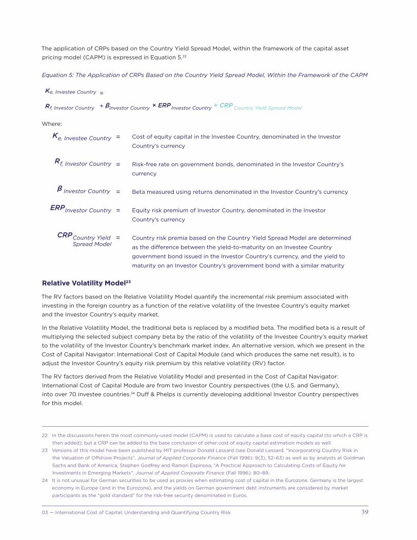
The application of CRPs based on the Country Yield Spread Model, within the framework of the capital asset

pricing model (CAPM) is expressed in Equation 5.22

Equation 5: The Application of CRPs Based on the Country Yield Spread Model, Within the Framework of the CAPM

K

R × ERPβ + CRP

=

+

e, Investee Country

f, Investor Country Investor Country Country Yield Spread ModelInvestor Country

Where:





=CRPCountry YieldSpread Model

Cost of equity capital in the Investee Country, denominated in the Investor

Country’s currency

Risk-free rate on government bonds, denominated in the Investor Country’s

currency


Equity risk premium of Investor Country, denominated in the Investor


Country risk premia based on the Country Yield Spread Model are determined

as the di�erence between the yield-to-maturity on an Investee Country

government bond issued in the Investor Country’s currency, and the yield to

maturity on an Investor Country’s grovernment bond with a similar maturity

eq: 5

Relative Volatility Model23

The RV factors based on the Relative Volatility Model quantify the incremental risk premium associated with

investing in the foreign country as a function of the relative volatility of the Investee Country’s equity market

and the Investor Country’s equity market.

In the Relative Volatility Model, the traditional beta is replaced by a modified beta. The modified beta is a result of

multiplying the selected subject company beta by the ratio of the volatility of the Investee Country’s equity market

to the volatility of the Investor Country’s benchmark market index. An alternative version, which we present in the

Cost of Capital Navigator: International Cost of Capital Module (and which produces the same net result), is to

adjust the Investor Country’s equity risk premium by this relative volatility (RV) factor.

The RV factors derived from the Relative Volatility Model and presented in the Cost of Capital Navigator:

International Cost of Capital Module are from two Investor Country perspectives (the U.S. and Germany),

into over 70 investee countries.24 Duff & Phelps is currently developing additional Investor Country perspectives

for this model.

22 In the discussions herein the most commonly-used model (CAPM) is used to calculate a base cost of equity capital (to which a CRP is

then added), but a CRP can be added to the base conclusion of other cost of equity capital estimation models as well.

23 Versions of this model have been published by MIT professor Donald Lessard (see Donald Lessard, “Incorporating Country Risk in

the Valuation of Offshore Projects”, Journal of Applied Corporate Finance (Fall 1996): 9(3), 52–63) as well as by analysts at Goldman

Sachs and Bank of America, Stephen Godfrey and Ramon Espinosa, “A Practical Approach to Calculating Costs of Equity for

Investments in Emerging Markets”, Journal of Applied Corporate Finance (Fall 1996): 80–89.

24 It is not unusual for German securities to be used as proxies when estimating cost of capital in the Eurozone. Germany is the largest

economy in Europe (and in the Eurozone), and the yields on German government debt instruments are considered by market

participants as the “gold standard” for the risk-free security denominated in Euros.


The use of RV factors based on the Relative Volatility Model within the framework of the CAPM model is slightly

different from the use of CRPs, as outlined previously. While CRPs are added to the base cost of equity capital,

RVs are multiplied by the equity risk premium (see Equation 6).25

Equation 6: The Application of RV Factors Based on the Relative Volatility Model, Within the Framework of the

CAPM

K

R × ERPβ × RV Factor

=

+

e, Investee Country

f, Investor Country Investor Country Relative Volatility ModelInvestor Country

Cost of equity capital in the Investee Country, denominated in the Investor


Risk-free rate on government bonds, denominated in the Investor Country’s

currency




Country risk premia based on the Country Yield Spread Model are determined

as the di�erence between the yield-to-maturity on an Investee Country

government bond issued in the Investor Country’s currency, and the yield to

maturity on an Investor Country’s grovernment bond with a similar maturity

Where:





=RV FactorRelative Volatility Model

Cost of equity capital in the Investee Country, denominated in the

Investor Country’s currency

Risk-free rate on government bonds, denominated in the Investor


Beta measured using returns denominated in the Investor Country’s

currency


Country currency

Relative Volatility Factors based on the Relative Volatility Model are

determined as the ratio of the annualized monthly standard deviation

of the Investee Country's equity returns (denominated in Investor

Country’s currency) relative to the annualized monthly standard

deviation of the Investor Country’s equity returns (denominated in

the Investor Country’s currency)

Case Study

This section provides a case study of a Canadian investor developing a cost of equity capital to be used in

the WACC for an investment located in Mexico, using the information found in the Cost of Capital Navigator:

International Cost of Capital Module.26

25 In the discussions herein the most commonly-used model (CAPM) is used to calculate a base cost of equity capital (to which an

RV adjustment is made), but an RV adjustment could potentially be made to the base conclusion of other cost of equity capital

estimation models as well.

26 The Cost of Capital Navigator: International Cost of Capital Module provides country-level equity risk premia (ERPs) for countries,

country risk premia (CRPs) developed using the Country Yield Spread Model and the Erb-Harvey-Viskanta Country Credit Rating

Model, and relative volatility (RV) factors developed using the Relative Volatility Model. This module can be used to estimate country-

level cost of equity capital globally, for up to 188 countries, from the perspective of investors based in any one of up to 56 countries

(depending on data availability). To learn more or to subscribe to the Cost of Capital Navigator: International Cost of Capital Module,

visit: dpcostofcapital.com.


Case Study Assumptions

In our case study:

• A Canadian investor plans to make an investment in Cyber Mexico, a company providing information

technology software and services in Mexico.

• Most of Cyber Mexico’s cash flows are generated in Mexico.

• The cash flow projections we have been given are in Mexican Pesos (MXN).

• A country risk premium (CRP) is considered appropriate.

The assumptions used in our case study are summarized in Exhibit 4.

Exhibit 4: Assumptions Used in Case Study27

Valuation DateCanadian Long-Term Risk Free Rate Mexican Tax Rate

March 31, 2018 3.50% 24%

Investor Country Canadian Industry Beta Cash Flow Projections

Canada 1.3 Mexico (MXN)

Investee Country Canadian Historical ERP Industry Sub-industry

Mexico 5.60% Information Technology Software and Services

In the following sections we will calculate cost of equity capital for Cyber Mexico.

The assumptions of our case study state that “most of Cyber Mexico’s cash flows are generated in Mexico”, and

that “the cash flows we have been given are in Pesos (MXN)”. The Canadian investor has determined there are no

sufficiently reliable inputs (e.g., risk-free rate, equity risk premium, beta) for the Investee Country (Mexico), and

has decided to develop a cost of equity capital estimate using inputs from a country for which reliable inputs are

available, and then translate that estimate into MXN using the International Fisher Effect.

This path is illustrated in Exhibit 5. Exhibit 5 is identical to Exhibit 1, except that the path that the Canadian investor

has decided to use to develop the discount rate estimates has been colored in Turquoise.28

27 Source of risk-free rate input: 2018 Valuation Handbook – International Guide to Cost of Capital, Appendix 3C, “Additional Sources of

Equity Risk Premium Data – Canada”, page 3C-10, as found in the “Resources” section of the Cost of Capital Navigator: International

Cost of Capital Module at dpcostofcapital.com. Duff & Phelps calculates estimates of “normalized” long-term risk-free rates for

the U.S., Canada, the U.K., and Germany (quarterly). Source of long-term equity risk premium input: Cost of Capital Navigator:

International Cost of Capital Module. The 5.6% used here is the historical average as measured over the 1919–2017 time horizon.

Additional Canadian long-term equity risk premia estimates are provided in the Cost of Capital Navigator: International Cost of

Capital Module, including: (i) an estimate (and underlying support analysis) based upon the research of Dr. Laurence Booth, Professor

of Finance and the CIT Chair in Structured Finance at the Rotman School of Management, University of Toronto, (ii) estimates from

Elroy Dimson, Paul Marsh, and Mike Staunton, authors of the Credit Suisse Global Investment Returns Yearbook 2019 (London: Credit

Suisse/ London Business School, 2019), and (iii) Pablo Fernandez, professor in the Department of Financial Management at IESE, the

graduate business school of the University of Navarra, Spain. All rights reserved. Used with permission.

28 The Canadian investor could have selected an alternative path. For example, this investor could have used future expected exchange

rates to convert the MXN cash flows to CAD. He or she would then need a discount rate also denominated in CAD to discount

these CAD-denominated cash flows. A solution would then be: (i) develop a discount rate using Canadian inputs, (ii) add a CAD-

denominated CRP, (iii) discount the CAD-denominated cash flows. This would result in a value conclusion denominated in CAD for

Cyber Mexico that incorporates the relative country risks of Mexico and Canada. If the Canadian investor then wanted to see the

value conclusion of Cyber Mexico in MXN, he could use the spot exchange rate to translate the value conclusion from CAD into MXN.

In Exhibit 5, this alternative path is equivalent to answering “Yes” to the question “Are cash flows in a mature currency?” and then

“Computing WACC in mature currency using available models to quantify CRP”.


Exhibit 5: A Framework for Valuing Businesses in Other Countries

Alternative 2: Reflect country risk in WACC

Are cash flows in a mature currency?*



If Investee Country currency needed:

Alternative 1: Use scenario analysis

Reflect di erent outcomes in cash flows

No CRP in WACC

Yes (Alt. 2)

Yes (Alt. 1)

*A “mature currency” is the currency of a countryfor which reliable cost of capital inputs are available.

Yes

No

NoIs Subject Company

exposed to country risk?

No CRP needed

Translate WACC into Investee Country currency using the

Internation Fisher E ect

In the Cost of Capital Navigator: International Cost of Capital Module, the Country Credit Rating Model is used to

calculate country risk premia for over 180 Investee Countries from 56 different investor perspectives, including

Canada. Canada has reliable risk-free rate, beta, and equity risk premium inputs available, so we will first develop

a cost of equity capital estimate for Cyber Mexico using (i) Canadian inputs, and (ii) the Country Credit Rating

Model.29

Estimating Cost of Equity Capital Using the Country Credit Rating Model Method

A summary of the steps needed is as follows:

• Develop cost of capital estimates using Investor Country (Canadian) inputs, which does have reliable

inputs available.

• Incorporate a measure of country risk (in this case, a CRP), in the cost of equity, and then

• Translate the estimate into the Investee Country’s currency (the Mexican Peso, or MXN) using the

International Fisher Effect.30

• Discount the MXN-denominated projected cash flows.

This results in a value conclusion denominated in MXN for Cyber Mexico that incorporates the country risks

of Mexico from a Canadian investor’s perspective. If the Canadian investor then wanted to see the value

conclusion of Cyber Mexico in CAD, the spot exchange rate could be used to translate the value conclusion from

MXN into CAD.

29 Later in this article the Country Yield Spread Model and the Relative Volatility Model are used to develop cost of equity capital

estimates for Cyber Mexico.

30 If the cash flows to be discounted are denominated in MXN, the discount rate must also be expressed in terms of MXN.


From Equation 4, the application of CRPs based on the country credit rating model within the framework of the

CAPM is:

K

R × ERPβ + CRP

=

+

e, Investee Country

f, Investor Country Investor Country Country Credit Rating ModelInvestor Country

Using the assumptions in Exhibit 4, we are using a Canadian long-term risk-free rate of 3.5% (normalized) and a

Canadian ERP of 5.6%, and have determined that the appropriate beta to use for a company in the Information

Technology Software & Services industry is 1.3. Substituting these values into Equation 4 gives us (with Canada

being the “Investor Country”):

K

3.5% + 1.3 X 5.6% + CRP

10.8% + CRP

=

=

e, Mexico (in CAD)

Country Credit Rating Model


The cost of equity capital estimate for a hypothetical company located in Canada and in the same industry as

Cyber Mexico is estimated at 10.8% (i.e., excluding the CRP adjustment for Mexico).31

The next step entails incorporating a country risk premium, since the actual subject company (Cyber Mexico)

is located in Mexico. As of the valuation date (March 31, 2018), the country risk premium for Mexico (from the

perspective of a Canadian investor in the context of the Country Credit Rating Model) is 4.1%.32

Substituting the 4.1% CRP value into the CAPM equation gives us:

K

K

K

10.8% + CRP

10.8% + 4.1%

14.9%

=

=

e, Mexico (in CAD)

e, Mexico (in CAD)

=e, Mexico (in CAD)


The cost of equity capital estimate for Cyber Mexico is estimated at 14.9%, expressed in CAD. This estimate

represents the risk of a hypothetical subject company located in Canada and in the same industry as Cyber Mexico

(10.8%), with an additional country risk premium of 4.1% added to adjust for the country risk of the actual subject

company, which is located in Mexico.33

The cost of equity capital estimate (14.9%) was developed using Canadian inputs (and is therefore in terms of

CAD) because reliable Mexican inputs (risk-free rate, equity risk premium, beta) were not available. However,

according to the assumptions of our case study, “most of Cyber Mexico’s cash flows are generated in Mexico”,

and “the cash flows we have been given are in Mexican Pesos (MXN)”.

31 For simplicity, the basic (i.e., “textbook”) CAPM is used here. Analysts may have additional risks that they deem necessary (e.g., size

premium, company specific risk, etc.).

32 Source: Cost of Capital Navigator: International Cost of Capital Module. To learn more or to subscribe, visit dpcostofcapital.com.

33 An implied assumption in this analysis is that what it “means” to be an “information technology software and services” company in

Canada means the same thing as being an information technology software and services company in Mexico. Some questions that

the analyst may wish to consider: (i) Are the risks of being a company operating in “Industry XYZ” in the Investee Country the same

as the risks of being a company operating in Industry XYZ in the Investor Country? (ii) Does a company operating in Industry XYZ in

the Investee Country have the same beta (β) as a company operating in Industry XYZ in the Investor Country? (iii) Does a company

operating in Industry XYZ in the Investee Country operate in a different industry environment from a company operating in Industry

XYZ in the Investor Country? (iv) Did the analyst apply any additional adjustments when the discount rate was developed for the

company operating in Industry XYZ as if it were located in the Investor Country? For example, was a size premium applied? “Large

company” and “small company” can mean very different things from country to country. For instance, a smaller-sized company in the

U.S. or Germany may be a “large” company in Estonia or Norway.


As previously discussed, a “common error” when dealing with cross-border valuations is mixing currencies. In

a DCF model, the numerator (expected cash flows) must be in the same currency as the denominator (which

includes the discount rate). So, either both the numerator and the denominator must be in CAD, or both must be

in MXN. The Canadian investor in our case study has decided to discount the MXN-denominated cash flows, so the

14.9% cost of equity estimate (currently in CAD) must be translated into MXN using the International Fisher Effect.

Using Equation 2, the application of the International Fisher Effect to translate the rates of return on equity would

result in the following relationship:

(1 + Inflation )

(1 + Inflation )



=

—CADMXN

CAD

MXN

If we assume that the expected long-term inflation rate for Mexico and Canada as of the valuation date (March 31,

2018) are 3.2% and 2.0%, respectively, then:34



(1 + 14.9%)

16.3%

=

=

MXN

MXN

(1 + 3.2%)

(1 + 2.0%)1× —

The cost of equity capital estimate for Cyber Mexico is estimated at 16.3%, expressed in MXN. This estimate

represents the risk of a subject company located in Mexico, in MXN, from the perspective of a Canadian investor.

Using Additional Models

As previously discussed, there is no single international cost of capital estimation model that is perfect. As such,

it is suggested that the analyst use the valuation data presented in the Cost of Capital Navigator: International

Cost of Capital Module to develop a range of indicated cost of equity capital estimates.35

In the following sections we estimate the cost of equity capital for Cyber Mexico using: (i) the Country Yield

Spread Model, and (ii) the Relative Volatility Model.

While the Country Credit Rating Model (used in the previous example) has 56 different Investor Country

perspectives (including Canada), the Country Yield Spread Model and the Relative Volatility Model have two

Investor Country perspectives: the U.S. and Germany. We can still use these two models to develop cost of capital

estimates for Cyber Mexico by using a “proxy” Investor Country perspective to develop cost of capital estimates,

and then translating the results into the desired currency using the International Fisher Effect.

Estimating Cost of Equity Capital Using the Country Yield Spread Model


• Develop cost of capital estimates using a Proxy Investor Country inputs (in this case, the U.S.),

which does have reliable inputs available.

34 Source of expected inflation estimates used in this example: IHS Markit’s long-term average CPI inflation forecasts for Canada and

Mexico dated March 15, 2018. For the purposes of the examples herein, expected inflation forecasts were calculated as the simple

average of IHS 2018 -2027 (10 years) annual forecasts for Canada and Mexico, in turn. In practice, the analyst may use longer time

horizons (or different data sources and/or methodologies) to estimate expected inflation. To learn more about IHS Markit, visit

https://ihsmarkit.com/company/index.html.






• Incorporate a measure of country risk (in this case, a CRP denominated in USD).

• Translate the estimate into the Investee Country’s currency (in this case, the Mexican Peso, or MXN)

using the International Fisher Effect.36

• Discount the projected MXN-denominated cash flows.

This results in a value conclusion denominated in MXN for Cyber Mexico. If the Canadian investor then wanted

to see the value conclusion of Cyber Mexico in CAD, the spot exchange rate could be used to translate the value

conclusion from MXN into CAD.

Using the U.S. as a “Proxy Investor Country” in the Country Yield Spread Model (see Equation 5), the application of

CRPs based on the Country Yield Spread Model within the framework of the CAPM is:

K

R

+ CRP

=

+

e, Investee Country

f, Proxy Investor Country

Country Yield Spread Model

× ERPβ Proxy Investor CountryProxy Investor Country

Substituting the U.S. long-term risk-free rate (3.5%, normalized), the Duff & Phelps Recommended U.S. ERP as of

March 31, 2018 (5.0%) and using the same beta (1.3) as of the March 31, 2018 valuation date into the Country Yield

Spread Model equation gives us:37

K 3.5% + 1.3 X 5.0% + CRP

10.0% + CRP

=e, Mexico (in USD)



=

The cost of equity capital estimate for a hypothetical company located in the U.S. (the Proxy Investor Country in

this example) and in the same industry as Cyber Mexico is estimated at 10.0% in USD.38


is located in Mexico. As of the valuation date (March 31, 2018), the country risk premium for Mexico (from the

perspective of a United States investor in the context of the Country Yield Spread Model) is 1.9%.39

Substituting the 1.9% CRP value into the CAPM equation gives us (with the U.S. being the “Proxy Investor Country”):

K

K

K

10.0% + CRP

10.0% + 1.9%

11.9%

=

=

e, Mexico (in USD)

e, Mexico (in USD)

=e, Mexico (in USD)


The cost of equity capital estimate for Cyber Mexico is estimated at 11.9%, expressed in USD. This estimate

represents the risk of a hypothetical subject company located in the U.S. and in the same industry as Cyber Mexico

(10.0%), with an additional 1.9% added to adjust for the country risk of the actual subject company, which is located

in Mexico.

36 If the cash flows to be discounted are denominated in MXN, the discount rate must also be in terms of MXN.

37 Duff & Phelps employs a multi-faceted analysis to estimate the conditional U.S. ERP that takes into account a broad range of

economic information and multiple ERP estimation methodologies to arrive at its recommendation. For details on the Duff & Phelps

recommended U.S. ERP over time, visit: https://www.duffandphelps.com/insights/publications/cost-of-capital.

38 For simplicity the basic (i.e., “textbook”) CAPM is used here. Analysts may have additional risks that they deem necessary to add in

specific analyses (e.g., size premium, company specific risk, etc.).



The cost of equity capital estimate (11.9%) was developed using U.S. inputs (and is therefore in terms of USD)

because reliable Mexican inputs (risk-free rate, equity risk premium) were not available. However, according to the

assumptions of our case study, “most of Cyber Mexico’s cash flows are generated in Mexico”, and “the cash flows

we have been given are in Mexican Pesos (MXN)”.

As previously discussed, in a DCF model, the numerator (expected cash flows) must be denominated in the

same currency as the denominator (which includes the discount rate). So, either both the numerator and the

denominator must be in USD, or both must be in MXN. The investor in our case study has decided to discount the

MXN-denominated cash flows, so the 11.9% cost of equity estimate (currently in USD) must be translated into MXN

using the International Fisher Effect.



(1 + Inflation )

(1 + Inflation )



=

—USDMXN

USD

MXN

If we assume that the expected long-term inflation rate for Mexico and the United States as of the valuation date (March 31, 2018) are 3.2% and 2.3%, respectively, then: 40

If we assume that the expected long-term inflation rate for Mexico and the United States as of the valuation date

(March 31, 2018) are 3.2% and 2.3%, respectively, then:40



(1 + 11.9%)

12.9%

=

=

MXN

MXN

(1 + 3.2%)

(1 + 2.3%)1× —


represents the risk of a subject company located in Mexico, in MXN, from the perspective of a U.S. investor.41

Estimating Cost of Equity Capital Using the Relative Volatility Model


• Develop cost of capital estimates using a Proxy Investor Country inputs (in this case, the U.S.), which does

have reliable inputs available.

• Incorporate a measure of country risk (in this case, a Relative Volatility (RV) factor denominated in USD).

• Translate the estimate into the Investee Country’s currency (in this case, the Mexican Peso, or MXN) using

the International Fisher Effect.42

• Discount the MXN-denominated cash flows.

This results in a value conclusion denominated in MXN for Cyber Mexico. If the Canadian investor then wanted

to see the value conclusion of Cyber Mexico in CAD, the spot exchange rate can be used to translate the value

conclusion from MXN into CAD.

40 Source of expected inflation estimates used in this example: IHS Markit’s long-term average CPI inflation forecasts for the U.S.

and Mexico dated March 15, 2018. For the purposes of the examples herein, expected inflation forecasts were calculated as the simple

average of IHS 2018 -2027 (10 years) annual forecasts for the U.S. and Mexico, in turn. In practice, the analyst may use longer time

horizons (or different data sources and/or methodologies) to estimate expected inflation. To learn more about IHS Markit,

visit https://ihsmarkit.com/company/index.html.

41 The Canadian investor may need to adjust for differences in expectations between those of a Canadian investor compared to a U.S.

investor, such as differences in expected ERP, etc.

42 If the cash flows to be discounted are denominated in MXN, the discount rate must also be in terms of MXN.


Using the U.S. as a “Proxy Investor Country” in the Relative Volatility Model (see Equation 6), the application of an

RV factor based on the Relative Volatility Model within the framework of the CAPM is:

K

R

× RV Factor

=

+

e, Investee Country

f, Proxy Investor Country

Relative Volatility Model

× ERPβ Proxy Investor CountryProxy Investor Country

Substituting the U.S. long-term risk-free rate (3.5%, normalized), the Duff & Phelps Recommended U.S. ERP as of

March 31, 2018 (5.0%) and using the same beta (1.3) as of March 31, 2018 valuation date into the Relative Volatility

Model equation gives us:43

K

3.5% + 1.3 X 5.0% × RV Factor

3.5% + 6.5% × RV Factor

=

=

e, Mexico (in USD)




is located in Mexico. As of the valuation date (March 31, 2018), the relative volatility factor for Mexico

(from the perspective of a United States investor) is 1.5.44

Substituting the 1.5 RV Factor value into the CAPM equation gives us (with the U.S. being the “Proxy Investor

Country”):

K

K

K

3.5% + 6.5% × 1.5

3.5% + 9.75%

13.3%

=

=

e, Mexico (in USD)

e, Mexico (in USD)

=e, Mexico (in USD)

The cost of equity capital estimate for Cyber Mexico is estimated at 13.3%, expressed in USD. This estimate

represents the risk of a hypothetical subject company located in the U.S. and in the same industry as Cyber Mexico,

with the excess return term multiplied by a ratio of 1.5 to adjust for the country risk of the actual subject company,

which is located in Mexico.

The cost of equity capital estimate (13.3%) was developed using U.S. inputs (and is therefore in terms of USD)

because reliable Mexican inputs (risk-free rate, equity risk premium) were not available. However, according to the

assumptions of our case study, “most of Cyber Mexico’s cash flows are generated in Mexico”, and “the cash flows

we have been given are in Mexican Pesos (MXN)”.

As previously discussed, in a DCF model, the numerator (expected cash flows) must be denominated in the

same currency as the denominator (which includes the discount rate). So, either both the numerator and the

denominator must be denominated in USD, or both must be in MXN. The investor in our case study has decided

to discount the MXN-denominated cash flows, so the 13.3% cost of equity estimate (currently in USD) must be

translated into MXN using the International Fisher Effect.

43 Duff & Phelps employs a multi-faceted analysis to estimate the conditional U.S. ERP that takes into account a broad range of

economic information and multiple ERP estimation methodologies to arrive at its recommendation. For details on the Duff & Phelps

recommended U.S. ERP over time, visit: https://www.duffandphelps.com/insights/publications/cost-of-capital.





(1 + Inflation )

(1 + Inflation )



=

—USDMXN

USD

MXN

If we assume that the expected long-term inflation rate for Mexico and the United States as of the valuation date

(March 31, 2018) are 3.2% and 2.3%, respectively, then:45

(1 + 3.2%)

(1 + 2.3%)Cost of Equity Capital


(1 + 13.3%)

14.3%

1×=

=

—MXN

MXN


represents the risk of a subject company located in Mexico, in MXN, from the perspective of a U.S. investor.46

Using this value as input in a DCF to discount the cash flows (which are denominated in MXN) results in a value

conclusion denominated in MXN for Cyber Mexico. If the Canadian investor wants to see the value conclusion of

Cyber Mexico in CAD, the spot exchange rate can be used to translate the value conclusion from MXN into CAD.

Summary of Cost of Equity Capital Estimates

In the preceding sections, we presented a case study of a Canadian investor developing a cost of capital estimate

for an investment located in Mexico using the information found in the Cost of Capital Navigator: International

Cost of Capital Module. More specifically, the case study focused on deriving cost of equity capital estimates for

our subject company, Cyber Mexico, using the three models available in the Cost of Capital Navigator (the Country

Credit Rating Model, the Country Yield Spread Model, and the Relative Volatility Model). A summary of these

estimates is shown in Exhibit 6. Note that in this particular case study, we did not focus on estimating the cost of

debt capital or the WACC for the subject company.

Exhibit 6: Summary of Cost of Equity Capital Estimates for Cyber Mexico (in MXN)

Model Cost of Equity Capital Estimate (%) (in MXN)

Country Credit Rating Model 16.3%

Country Yield Spread Model 12.9%

Relative Volatility Model 14.3%

45 Source of expected inflation estimates used in this example: IHS Markit’s long-term average CPI inflation forecasts for the U.S. and

Mexico dated March 15, 2018. For the purposes of the examples herein, expected inflation forecasts were calculated as the simple

average of IHS 2018 -2027 (10 years) annual forecasts for the U.S. and Mexico, in turn. In practice, the analyst may use longer time

horizons (or different data sources and/or methodologies) to estimate expected inflation. To learn more about IHS Markit, visit

https://ihsmarkit.com/company/index.html.

46 The Canadian investor may need to adjust for differences in expectations between those of a Canadian investor compared to a U.S.

investor, such as differences in expected ERP, etc.


Cyber Mexico’s cost of equity capital falls in a range of 12.9% (the low estimate) to 16.3% (the high estimate),

with an average and median estimate of 14.5% and 14.3%, respectively. The specific facts and circumstances of

the subject business, asset, or project being evaluated, coupled with the judgment of the analyst, will determine

whether the actual cost of equity capital falls in the upper, middle, or lower part of the indicated range.

Using these conclusions (which are in terms of MXN) in a DCF to discount the cash flows (which are also

denominated in MXN) results in a value conclusion denominated in MXN for Cyber Mexico. If the Canadian investor

wants to see the value conclusion of Cyber Mexico in CAD, he could use the spot exchange rate to translate the

value conclusion from MXN into CAD.

Key Things to Remember About International Risk and Cost of Capital

• Due to the trend toward globalization, there may be less theoretical justification for country risk premia

than may have been warranted even a few decades ago. However, these risks still exist in the real world,

and it would likely be unwise to make investment decisions without considering these incremental risks.

• The risks associated with international investing can largely be characterized as financial, economic, or

political. These risks can include: (i) regulation that restricts foreign investment, (ii) taxation differences,

(iii) legal factors, (iv) information deficiencies, (v) trading costs, (vi) political instability, and (vii) physical

barriers, among others.

• There is no consensus among academics and practitioners as to the best model to use in estimating

the cost of equity capital in a global environment. None are perfect. Understanding the strengths and

weaknesses of the available models is important. Employing multiple methods may be prudent.

• In choosing a model, the goal is to balance several objectives: (i) acceptance and use, (ii) data availability,

and (iii) simplicity.

• Cash flows generated in foreign currency and country risk may have a significant impact in a valuation.

• Currency used to project cash flows MUST always be consistent with the currency of the discount rate.

Not doing so is a common error.

• The Cost of Capital Navigator: International Cost of Capital Module provides country-level equity risk

premia (ERPs) for 16 countries, country risk premia (CRPs) developed using the Country Yield Spread

Model and the Erb-Harvey-Viskanta Country Credit Rating Model, and relative volatility (RV) factors

developed using the Relative Volatility Model. The Cost of Capital Navigator is an online tool that can

be used to estimate country-level cost of equity capital globally, for up to 188 countries, from the

perspective of investors based in any one of up to 56 countries (depending on data availability).47

To learn more or to subscribe to the Cost of Capital Navigator: International Cost of Capital Module,

please visit dpcostofcapital.com.





Documents

International Cost of Capital - Understanding and