Embed Size (px)
Citation preview
Faculty of Business and Law
SCHOOL OF ACCOUNTING, ECONOMICS AND FINANCE
School Working Paper - Economic Series 2006
SWP 2006/13
INTERNATIONAL COMPARISONS OF RURAL‐URBAN EDUCATIONAL ATTAINMENT:
DATA AND DETERMINANTS
Mehmet A. Ulubaşoğlu and Buly A. Cardak
First Version: December 2004 This Version: August 2006
The working papers are a series of manuscripts in their draft form. Please do not quote without obtaining the author’s consent as these works are in their draft form. The views expressed in this paper are those of the author and not necessarily endorsed by the School.
1
INTERNATIONAL COMPARISONS OF RURAL‐URBAN EDUCATIONAL ATTAINMENT:
DATA AND DETERMINANTS†
Mehmet A. Ulubaşoğlu* Buly A. Cardak±
First Version: December 2004 This Version: August 2006
Abstract
We study cross‐country differences in rural and urban educational attainment by using a data set for a diverse group of 56 countries. Utilizing human capital, labor market and migration theories, we identify national, rural and urban factors that are expected to influence rural and urban households in their educational choices. We apply our theoretical arguments to a dataset that we construct from data available in UNESCO Educational Yearbooks (1964‐1999). We find that improved access to labor markets and lower risks associated with human capital investment reduce the disparities in the ratio and the levels of rural and urban schooling years. Importantly, countries with higher amount of resources and with better institutional framework to allocate such resources have lower rural‐urban inequality in education. We also find that the impact of credit availabilities, type of legal system, geography and religion on the rural‐urban educational inequality are related to the level of economic development. JEL Classification: I20, O18, R12.
Keywords: Human Capital, Economic Geography, Rural and Urban Educational Inequality, Political and Legal Institutions.
† We would like to thank Nejat Anbarci, Prasad Bhattacharya, Hristos Doucouliagos, Monica Escaleras, Phillip Hone, Jean‐Pierre Laffargue, Pushkar Maitra and Dimitrios Thomakos for their valuable comments in the earlier drafts of this paper. Any remaining errors are our own. * School of Accounting, Economics and Finance, Deakin University, 221 Burwood Highway, Burwood, Victoria 3125, Australia. e‐mail: [email protected]. ± Corresponding author: Department of Economics and Finance, La Trobe University, Bundoora, Victoria 3086, Australia. e‐mail: [email protected].

2
1. INTRODUCTION This paper studies cross‐country differences in rural and urban educational attainment by using a dataset for a diverse group of 56 countries. Using human capital, labor market and migration theories, we identify national and rural‐urban factors that are expected to influence rural and urban households and individuals in their educational decision making. We apply our theoretical arguments to a dataset that we construct from data available in UNESCO Educational Yearbooks (1964‐1999). In our empirical analysis, we use the ratio of rural to urban average schooling years to study rural‐urban educational inequality, while we also investigate cross‐country variation in the levels of rural and urban educational attainment. The rural‐urban divide has been a major area of study in development economics, focusing on divisions along rural‐urban lines within countries, particularly with respect to industrialization (Kuznets, 1955, 1973). In more recent times, studies on rural‐urban issues have focused on economic geography, and its links to migration, urbanization, trade and economic growth (see Williamson 1988, Shukla 1996, Fujita et al. 1999, Henderson 2005). While numerous studies have considered the rural‐urban educational divide within a single‐country, there has been limited research on this issue across countries.1 Thus, our paper unifies two existing literatures: i) the survey based studies that consider rural‐urban differences in educational attainment within single countries (for example Kochar (2004) considers India, Knight and Li (1996) consider China and Al‐Samarrai and Reilly (2000) and Barnum and Sabot (1977) both consider Tanzania), and ii) the cross country studies employing average national educational attainment (for example de Gregorio and Lee (2002)). In doing this, we are attempting to provide a unified explanation of cross country differences in rural‐urban educational inequality. Barro and Lee (1993, 1996, 2001) are pioneers in providing researchers with comprehesive cross‐country data sets on national educational attainment, the most recent covering the period 1960‐2000 and 142 countries.2 While the Barro and Lee datasets, which are based on UNESCO Educational Yearbooks, cannot be decomposed to create a panel of rural and urban schooling, sufficient data exists in that source to construct an unbalanced panel data set of rural and urban educational attainment across countries. This is critical as our cross‐country analysis would not be possible without this data. Our dataset comprises a diverse range of countries from the most developed to some of the least developed. Another feature of our dataset is that we have further disaggregated rural and urban educational attainment
1 Sahn and Stifel (2003) compare a number of living standard measures (of which educational attainment is one) across the rural‐urban divide for 24 African countries. 2 While Barro and Lee (1993, 1996, 2001) were the first to create large cross‐country data sets on national average years of schooling, Nehru et al. (1995) and de la Fuente and Domenech (2001) offer alternative data sets at the national level, suggesting a growing interest in such data. We expand the diversity of data sets through disaggregation at the regional level.

3
into male and female attainment within each region, though we do not exploit this distinction econometrically in this paper.3 In the empirical analysis, we model the ratio and the levels of rural vs urban schooling years by using economic, demographic, political, cultural, geographic, gender and infrastructural variables, estimating reduced form equations with General–to‐Specific and Specific‐to‐General modelling techniques, and subjecting our results to a range of statistical tests. As educational inequality across regions is an extremely important development issue, we place more emphasis on the results for the ratio of rural‐urban schooling. We find that countries with greater resources and those with more effective channels to allocate these resources have less rural‐urban educational inequality. Such distributional channels seem to be influenced by institutional framework such as the legal system within a country, colonial history, political stability as well as geographical characteristics such as being landlocked and/or a larger country. For instance, countries with French legal system, on average, have higher rural‐urban inequality, while the reverse is true for countries with British legal system. Also, countries with colonial past in general, and the countries with post‐war independence in particular have higher rural‐urban inequality. This may be related to the extractive rather than settlement nature of colonies gaining independence in the postwar period; see Acemoglu et al. (2001). In addition, countries with less stable political environments, that are landlocked and those with larger surface areas have higher rural‐urban inequality, suggesting that such factors negatively influence effective allocation of resources across regions, other things being equal. We also find that rural‐urban educational inequality is lower in economies with larger formal labor markets and better infrastructure, while greater risks associated with human capital investment lead to greater rural‐urban educational inequality. Our results also show that the strength of these mechanisms depends on the level of economic development. In particular, the impact of credit availability, type of legal system, geography and religion on rural‐urban inequality changes with the level of development in a country. Two particularly interesting examples of such results include that a legal system of French (British) origin is negatively (positively) related to rural‐urban educational inequality in less developed economies, while the reverse is found in wealthier, more developed economies. In light of recent findings by Grier (1999) on the link between colonial history, education and economic performance and the robust impact of human capital on economic growth (Doppelhofer, Miller and Sala‐i‐Martin 2004), our results suggest rural‐urban human capital accumulation, and the disparities between regions, may be another mechanism through which colonial heritage and institutions influence long run economic performance.4 3 While our focus is understanding cross‐country differences in rural and urban educational attainment, we expect that our newly assembled dataset on rural‐urban schooling years will be useful to researchers wishing to explain cross‐country phenomena such as economic growth, inequality, employment and migration. To this end, the data are presented in Table 1. 4 For some other mechanisms, see Acemoglu et al. 2001 and La Porta et al. 1998, 1999.
4
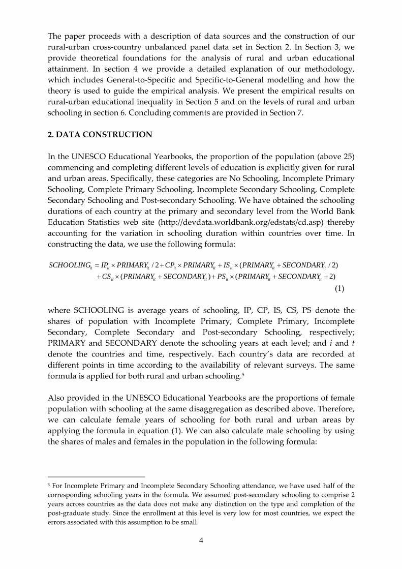
The paper proceeds with a description of data sources and the construction of our rural‐urban cross‐country unbalanced panel data set in Section 2. In Section 3, we provide theoretical foundations for the analysis of rural and urban educational attainment. In section 4 we provide a detailed explanation of our methodology, which includes General‐to‐Specific and Specific‐to‐General modelling and how the theory is used to guide the empirical analysis. We present the empirical results on rural‐urban educational inequality in Section 5 and on the levels of rural and urban schooling in section 6. Concluding comments are provided in Section 7. 2. DATA CONSTRUCTION In the UNESCO Educational Yearbooks, the proportion of the population (above 25) commencing and completing different levels of education is explicitly given for rural and urban areas. Specifically, these categories are No Schooling, Incomplete Primary Schooling, Complete Primary Schooling, Incomplete Secondary Schooling, Complete Secondary Schooling and Post‐secondary Schooling. We have obtained the schooling durations of each country at the primary and secondary level from the World Bank Education Statistics web site (http://devdata.worldbank.org/edstats/cd.asp) thereby accounting for the variation in schooling duration within countries over time. In constructing the data, we use the following formula:
)2()()2/(2/
++×++×++×+×+×=
itititititit
itititititititit
SECONDARYPRIMARYPSSECONDARYPRIMARYCSSECONDARYPRIMARYISPRIMARYCPPRIMARYIPSCHOOLING
(1) where SCHOOLING is average years of schooling, IP, CP, IS, CS, PS denote the shares of population with Incomplete Primary, Complete Primary, Incomplete Secondary, Complete Secondary and Post‐secondary Schooling, respectively; PRIMARY and SECONDARY denote the schooling years at each level; and i and t denote the countries and time, respectively. Each country’s data are recorded at different points in time according to the availability of relevant surveys. The same formula is applied for both rural and urban schooling.5 Also provided in the UNESCO Educational Yearbooks are the proportions of female population with schooling at the same disaggregation as described above. Therefore, we can calculate female years of schooling for both rural and urban areas by applying the formula in equation (1). We can also calculate male schooling by using the shares of males and females in the population in the following formula:
5 For Incomplete Primary and Incomplete Secondary Schooling attendance, we have used half of the corresponding schooling years in the formula. We assumed post‐secondary schooling to comprise 2 years across countries as the data does not make any distinction on the type and completion of the post‐graduate study. Since the enrollment at this level is very low for most countries, we expect the errors associated with this assumption to be small.

5
POPMALESCHOOLINGMALEPOPFEMALESCHOOLINGFEMALESCHOOLINGTOTAL _____ ×+×=
(2) where female_pop and male_pop are the shares of female and male populations above 25 in the society, respectively. The data on the rural‐urban divide in the female and total population are presented in Table 1.6 Descriptive statistics on rural and urban attainment are presented in Tables 2a through 2d. The comparability of the data per se is limited since we have data for different countries in different years. Thus, we compare the data of developing and developed countries, classified for each decade from 1950‐1990, and these statistics are presented in Table 2e. The data set spans countries from various development levels, providing a good source of variation for empirical analysis. To assess the reliability of our construction of the data and its compatibility with the existing data sets, we compare the “national” average years of schooling that we calculate from our rural and urban educational attainment (weighted by respective populations of age 25 years or more) with that of Barro and Lee (2001).7 The correlation is found to be 0.95. All statistics show strong similarities between the two measures. Statistical tests fail to reject the equality of means and medians. These minor discrepancies seem reasonable in the light of the fact that Barro and Lee, i) have time series observations available on national schooling enrolments, ii) take into account population growth (by looking at national birth and mortality rates) to approximate the enrolment of each age group, and iii) use gross enrollment rates, adjusted for repeaters, while such features are not available for our data. 3. THEORETICAL FRAMEWORK FOR THE ANALYSIS OF RURAL‐URBAN SCHOOLING Schooling decisions and the subsequent educational attainment are typically household and individual choices, which are subject to various constraints such as mandatory schooling and credit availability. Haveman and Wolfe (1995) outline three broad classes of factors that determine educational attainment; (i) environmental and social factors (largely affected by government), (ii) within‐household decisions and allocations (typically made by parents) and (iii) individual choices made by the student. They posit that in this line of reasoning, government moves first, making some direct investments and establishing the environment in which parents and children make their choices. Given this environment, parents decide on their work and earnings, time and resources spent on children, family structure and location, all of which affect their children. Lastly, children, given their talents, resources devoted
6 The data on rural‐urban male educational attainment are available upon request; we, however, present the descriptive statistics for those calculations. 7 See Table 2b. This comparison is based on the countries and years with data available to us and the data of the corresponding year in the Barro and Lee data set. As their data set is in 5‐year intervals, we use straight‐line interpolation to approximate the data of a specific year in their data set.
6
to them, and the social and parental incentives they face, make their own choices about education. Our objective, however, is to focus on rural‐urban differences in educational attainment in a cross country framework. We do this by considering environmental and social factors that shape educational outcomes and their differences within and between countries. The ideas behind our empirical study are that individuals react to national and rural‐urban characteristics in making their education choices, and schooling years evolve accordingly. The Haveman‐Wolfe structure can guide us in forming the theoretical and empirical frameworks for the analysis. We focus on human capital and labor market theories and the possibility of returns to human capital investment, through formal education, given the labor market environment. A simple, though somewhat stylized, way to think about our approach is that households face the choice of their children supplying labor to the family farm and subsisting, both during schooling years and beyond, or alternatively foregoing some farm labor during school years and supplying labor on the formal labor market in the long run. The possibility of such choices is limited by mandatory schooling requirements. However, even in the presence of mandatory schooling, the amount of time and resources devoted to education is at the discretion of the household, conditional on the institutional structures that enforce such rules and how strictly they are applied.8 The key point is that the likelihood of parents and students investing in human capital through formal schooling will be determined by the potential for such investment to earn a greater return than the best alternative. This will be affected not only by the level of economic development within a country but by the differences in development and opportunities between rural and urban areas within countries and the way that nation‐wide factors influence both rural and urban households.9 The following theoretical arguments are expected to underpin the cross‐country differences in the ratio and the levels of rural and urban schooling years. 3.1 Riskiness of the Investment From the perspective of the household and the student, investment in human capital through formal schooling entails uncertainty. For the household, this might be the risk of child mortality, and for the student, it might be related to demand for skilled labor in local areas ensuring a reasonable return on investment. We expect that differences in demographic characteristics such as health and death rates as well as political environments and institutions that enforce contracts and protect property rights will influence the probability of children completing a schooling program and
8 In Turkey, for instance, mandatory schooling of five years has applied since 1923 (with its origins dating back to 1876 in the Ottoman period), however, we find average years of schooling of 4.3 at the national level and 3.3 years in rural areas in 1990. This is consistent with observations for other countries in our sample. 9 Barro (1991) emphasizes the importance of national characteristics by implying that the individual return to ability (or education) is higher if the population is generally more able (or educated).

7
supplying labor on the market. The lower this probability, the less inclined households will be to invest in the human capital of their children. We interpret data about health, type of legal system and political environment as providing some empirical evidence on the differences in the riskiness of human capital investment, both across countries and across rural and urban areas. The data we have in this category include: (i) Demographic and infrastructural variables such as national life expectancy,10 rural and urban death rates and doctors availability. The intuition behind these variables is that the longer is life expectancy and the lower the death rate, the greater the expected benefit to the household of investing in human capital; and (ii) Political and institutional variables such as type of legal system (British, French, German, Scandinavian and Socialist), the standard of political rights and civil liberties, and the average number of revolutions, coups and assassinations. Laws pertaining to investor protection are investigated by La Porta et al. (1998) who find that French‐civil‐law countries provide the weakest protection to investors, while British‐common‐law countries the strongest. German and Scandinavian‐law countries generally fall between these two. La Porta et al. (1999) argue that countries that have a British legal system (common law) enforce contracts in a more practical way, with implications for credit availability, business formation and long‐run growth, whereas a French legal system imposes bureaucratic burden on economic activities. We expect that greater investor rights and protections will lower the risks associated with investment in physical capital and lead to substitution away from human into physical capital. However, we also expect that a legal system that is more conducive to investment in physical capital will also encourage investment in human capital; see Acemoglu et al. (2001) and references therein. The overall effect is an empirical question to be identified below. 3.2 Labor Markets It is no secret to development economists that countries, and rural and urban regions within, differ in the operation of their labor markets. The role of agriculture in the economy, and the employment, organization, payment structure and other distinct features of this sector can affect the education choices of households and students. If agriculture is primarily for subsistence, the required human capital can be acquired without formal schooling.11 Similarly, the role of non‐farm production, heterogeneity of the products produced and technological features thereof, seasonal continuity and geographically contained production structures can differ across urban areas (Rosenzweig, 1988). If non‐farm employment prospects are significant, the expected benefits of formal schooling would be greater as would educational attainment. In addition, real wages and price levels are generally higher in urban than in rural areas (Schultz, 1988); this may account for the relative differences in educational returns and costs in rural and urban areas. Moreover, returns to schooling in rural areas may
10 We address the use of national variables in sections 4.1. and 6.3. 11 There is empirical evidence that farmers with more education are more productive and earlier to adopt new farming techniques and technologies, see Schultz (1988, p. 597).
8
be lower due to the “less dynamic agricultural technology that creates lower opportunities for the educated worker” (Jamison and Lau, 1982). Of the data we have, economic variables include agricultural vs. nonagricultural value added per worker (to approximate income and productivity), arable land per capita (to approximate relative factor returns) and the proportion of female teachers to total teachers (to proxy for non‐agricultural labor market opportunities). We expect higher levels of female teachers to lead to higher rural educational attainment because of greater labor market opportunities for both men and women. Demographic data include rural and urban birth rates (to approximate average household size and congestion in schools) and rural population density, and geographical data include latitude (weather conditions and rainfall) and surface area of the countries. These geographical variables are included because we expect them to influence the productivity of land in agriculture, thereby affecting the size of formal labor markets and making education more or less attractive. It is also argued that natural resource endowments and the latitude can affect government policies and institutions that underlie the business environment, thereby influencing formal labor markets and the value of education; see Acemoglu et al. (2001) and Easterly and Levine (2003). 3.3 Labor Mobility and Intersectoral Migration As suggested above, demand for formally educated labor will influence households and individuals in their willingness to invest in human capital. Often, the demand for such labor might be far from rural centers, implying transport infrastructure and migration patterns might have something to say about differences in educational attainment between rural and urban areas.12 When making a decision about investing in human capital through formal schooling, the prospects of being able to take the acquired human capital to market is important and the more costly this is likely to be for rural residents, the less likely they will be to invest in human capital, relative to their urban counterparts. Schultz (1988) points out that accumulating human capital in rural areas has a potentially lower time cost and since the return in urban centers is typically higher, migration is one way to boost returns. While we are not focusing on the rate of return to schooling here, we are concerned about migration and its potential to contaminate data on where actual education is acquired. We interpret the following data to measure either the ability or willingness of citizens to move around their country in order to access labor markets: economic data such as intersectoral migration; geographical variables such as total surface area, latitude of the countries (distance from the equator), and landlocked and island dummies; demographic variable, ethnic fractionalization; infrastructural variable, telephone line availability; political variables such as number of assassinations, coups and revolutions. Larson and Mundlak (1997) argue that countries that are ethnically fractionalized, with lower political freedom and stability and larger geographical
12 For a study of the interaction between rural and urban labor markets and their implications for education in India, see Kochar (2000) and Kochar (2004).
9
area are less likely to experience migration, thereby lowering returns and discouraging rural education. Also, Easterly and Levine (1997) show that ethnic diversity reduces the provision of public goods like physical infrastructure and national education, thereby reducing the mobility of labor and discouraging rural educational attainment. It is also argued, however, that political instability leads governments to discourage rural‐urban migration in order to reduce political and social unrest in the seat of power, see for example Davis and Henderson (2003) and Ades and Glaeser (1995). This will reduce opportunities for human capital in urban markets and discourage rural relative to urban educational attainment. Lattitude is expected to play a role because the further from the equator, the more problematic travel can be in winters, thereby reducing mobility. Landlocked countries are generally mountainous and do not have sea based transport, restricting mobility within such countries. Conversely islands depend heavily on sea transport and are likely to experience enhanced mobility. Improved telecommunication infrastructure reflects lower (non‐economic) costs for migrating labor, thereby encouraging mobility and rural educational attainment. 3.4 Credit Constraints It is highly likely that parents and children seeking formal schooling would, at least partially, lack funds to finance the costs of attending a school program; Saint Paul and Verdier (1993). Thus, differences in credit availabilities and the distribution of assets used to credibly borrow could explain cross‐country and inter‐regional differences in educational attainment. Economic variables such as land Gini, the share of education expenditures in GDP and M2/GDP can be interpreted to be capturing these effects. We also use a German legal system dummy, as financial systems of German origin are known to be strict but efficient in allocating credit; see for example Aoki et al. (1995, chapter 4) who point out that creditors play an important monitoring role in the Japanese financial system which has similiarities to the German system, see also Deeg (1998) and Vitols (1998) who discuss the characteristics of the German banking system.13 In the political economy literature, land Gini is mostly used as a proxy variable for cross‐country differences in asset distribution; see Deininger and Olinto (2000). We use it, however, as a proxy for income distribution, because we expect land distribution to be closely tied to income distribution particularly in rural areas. We expect greater rural income inequality to reduce rural educational attainment relative to urban educational attainment. The monetary measure M2/GDP is typically used to approximate credit availabilities and financial constraints in an economy; see Benhabib and Spiegel (2000). Again, the tighter is credit availability, the less scope for households to access education. 3.5 Infrastructure
13 Countries with a German based legal system in our sample are Japan and South Korea.
10
Infrastructure and its availability is a general development issue and as such is likely to play a role in educational choices and outcomes. In terms of our descriptive modelling of rural and urban education, infrastructure will primarily operate through the mechanisms we have outlined above; investment risk, labor markets, labor mobility and migration, and credit constraints. Behrman and Birdsall (1983) argue returns to schooling in rural areas may be lower due to lower quality of schools. In terms of educational infrastructure, we have data on primary school pupil‐teacher ratios while we also use the ratio of rural‐urban birth rates to proxy for for rural‐urban differences in congestion in schools.14 More general infrastructure measures available to us include telephone line availability, fertilizer consumption and tractor availability and a colonization dummy which controls for infrastructural and institutional inheritances from colonial powers as in Acemoglu et al. (2001) and La Porta et al. (1999).15 We expect greater infrastructure to improve the opportunities for human capital and therefore raise educational attainment, especially in rural regions. 3.6 Other Factors We also consider a number of cultural control variables such as religion variables and the ratio of female pupils to male pupils in primary and secondary public and private schools (girl‐boy student ratio). We include Catholic, Protestant and Confucian16 religion variables to control for differences in national attitudes to education based on religious practices, as some religions may be more open to the education of girls or higher education than others. The girl‐boy student ratio is intended to control for differences in cultural attitudes to the education of girls and boys and a more conservative attitude to education in general, possibly reflecting differences in attitudes towards education between rural and urban areas. Its inclusion is consistent with Sahn and Stifel (2003) who find that girl‐boy student ratio is lower in rural areas.17 4. ECONOMETRIC FRAMEWORK FOR THE ANALYSIS OF RURAL‐URBAN SCHOOLING We have a range of intuitively appealing data at the rural, urban and national levels to identify the data generating process (DGP) behind the levels of rural and urban schooling and their ratio (henceforth, RATIO). Detailed data definitions and their sources are provided in Appendix A, with summary statistics presented in Table 3.
14 We would prefer to use the ratio of rural to urban pupil/teacher ratio but such disaggregated data is unavailable. 15 We do not use data on time held as a colony, however, Grier (1999) finds that colonies held for longer periods tend to perform better on average. 16 Three countries in our sample are Confucian: Japan, South Korea and China (the latter was listed in the “other” category of religions in La Porta et al. (1999), as Japan and Korea. We have named this category as Confucian as a general name for East Asian teachings and approach to education. 17 Note that we use girl‐boy student ratio and girl‐boy ratio interchangably throughout the paper.

11
Note that the explanatory variables are measured as five year averages (i.e., 1970‐74, 1975‐79, etc).18 For instance, rural and urban educational attainment data for Chile are recorded for 1970, and we use the independent variables from the 1970‐1974 period.19 Establishing the econometric framework entails an interactive blend of theory and evidence.20 More specifically, in our modelling approach, we utilize both the empirical evidence that arises en route as well as the afore‐mentioned theoretical guidance. This leads us to two approaches: general‐to‐specific (GTS) and specific‐to‐general (STG) modelling. 4.1 Some Issues on Explanatory Variables in Modelling It is important to note some points about the explanatory variables. We have two types of variables. The first type are region‐specific variables, where rural vs urban decomposition is available, such as agricultural and nonagricultural value added per worker and rural and urban birth rates. In the RATIO models, we employ the ratios of such variables, while the levels of such variables are employed in the models of the levels of rural and urban schooling. The second type are national variables. We make a further distinction within this class of variables: i) ‘truly’ national variables (e.g., landlocked, political rights), which are not likely to differ across rural and urban areas, and ii) those that could be decomposed into rural‐urban values (e.g., pupil‐teacher ratio), but whose decompositions are not available. National variables are employed in the models of both the ratio and the levels of rural‐urban schooling. While truly national variables do not differ across regions, the influence that they exert on each region may be quite different. In particular, the impact on rural and urban schooling may vary with the level of economic development, a hypothesis that will
18 This is expected to reduce the measurement error that might exist in the explanatory variable data. Also, the “Aliasing the time series” problem (see Hamilton 1994) is expected to be minimal in this case as we are modelling a relatively slow changing variable such as average educational attainment. 19 We assume that three data points of the 1950s (i.e., on Finland, France and Norway) belong to 1960‐64. Two observations of Afghanistan (1975 and 1979) are averaged to use explanatory variables from the 1975‐79 period. 20 Note that we can at most approximate the DGP, as whatever models we form would be the reduction of the true DGP due to the sampling process, data unavailability or the measurement of available data. 24 Ideally, we would like to have access to many national data disaggregated to the regional (rural and urban) level. This would improve the empirical analysis and enhance our understanding of the rural versus urban educational attainment. Unfortunately, a wide variety of such data such as rural and urban unemployment data for a large number of countries is not readily available.
12
be tested in Section 5.2. For potentially decomposible variables there may be differences between rural and urban areas, but the data for a rural‐urban decomposition are unavailable.24 Thus, some of these variables proxy national resources in the RATIO models, while they are used as proxies for their rural‐urban counterparts in the levels models. We check the reliability and implications of the latter approach in Section 6.3. 4.2. General‐to‐Specific Modelling: Data‐driven approach General‐to‐specific modelling involves the formation of a general unrestricted model (GUM) with several explanatory variables, and testing it down by eliminating insignificant variables to arrive at a final model in which all variables are significant. Hendry defines a GUM as “the most general, estimable, statistical model that can reasonably be postulated initially, given the present sample of data, previous empirical and theoretical research, and any institutional and measurement information available” (1995, p. 361). In essence this process is driven by the data. The Haveman‐Wolfe structure, however, can help us with the initial steps of the search process. The GUM should include the objectives, opportunities and constraints‐related conrol variables, and in fact many of these variables can also be linked to the labor market, human capital and migration theories. Thus, we use economic, demographic, political, cultural, geographic and infrastructure‐related variables in the general regression. The regression takes the following form:
itititit
itititit
CULTURALGEOGRAPHICPOLITICALTURALINFRASTRUCCDEMOGRAPHIECONOMICSCHOOLINGREG
εααααααα
+++++++=
654
3210_
(4) where the variables on the right‐hand side derive from the relevant categories and REG_SCHOOLING is one of the three dependent variables: RATIO, rural or urban schooling levels. Each category includes three to four variables, so that the general regressions are run with around 20 variables. A general model for RATIO is presented in Table 5. We sequentially delete one or a group of insignificant variables from this model by using F‐tests, starting from the most insignificant(s) to the least, leading to the Specific model presented in the next column. The GTS modelling for RATIO produces a narrow group of explanatory variables. We find that relative productivity is positively related to RATIO. The estimated coefficient 0.768 implies that, ceteris paribus, there would be a 0.40 points difference in the RATIO values of Nepal and Canada, which possess the lowest and the highest relative productivity values in our sample, respectively, both belonging to the 1980‐84 period.25 We also find that telephone availability (per 1,000 people) is positively associated with RATIO. Its coefficient, 0.001, implies that this variable can explain 0.38 points of the difference in the RATIO values of Mali and Canada in the 1975‐79 period (which are recorded to have 0.6 and 375.7 phones per 1,000,
25 Such cross‐country comparisons can be made across the same time periods.
13
respectively, with Mali’s figure being the lowest in our sample, and Canada having one of the highest). The model also suggests that countries with colonial past have, on average, 0.12 lower RATIO points than those with no colonial history. Likewise, countries with a legal system of French origin have, on average, 0.17 lower RATIO points than those with a non‐French system, other things being equal. These results are with important implications and will be discussed further below. Lastly, we find that catholic populations tend to have less rural‐urban inequality. The coefficient estimate 0.002 implies that, ceteris paribus, a country with exclusively catholic population has about 0.20 higher RATIO than a country with no catholic population. For rural schooling, the significant variables of the specific model are arable land per capita (+), rural birth rate (‐), fertilizer consumption (+), colony (‐), landlock (+) and French legislation (‐) dummies, the share of protestants in the population (+) and the girl‐boy ratio (+). In parentheses are the signs of the estimated coefficients, which are consistent with economic intuition. For urban schooling, we have again fewer variables in the specific model. These include, life expectancy (+), urban birth rate (‐), landlock dummy (+) and girl‐boy ratio (+). While the signs are consistent with intuition, we are surprised by how few of these variables are statistically significant in explaining urban educational attainment. 4.3. Specific‐to‐General Modelling: Theory‐driven approach We feel the need to analyze the data further for several reasons: i) Multicollinearity may arise in these models because most explanatory variables are development‐related and very likely to be correlated with each other. Thus, in some cases some relevant variables may initially appear as insignificant and hence be incorrectly omitted; ii) Importantly, there might be several economic mechanisms driving rural‐urban educational attainments, which suggests an approach motivated by theory. To address these issues simultaneously, one solution is to conjecture the potentially relevant processes with the help of theory and attempt our modelling at a smaller scale. In this vein, we estimate equation (4) with each category having only one representative variable. This can mitigate the multicollinearity problem, while keeping the explanatory power of the models relatively high, as between‐category correlation is expected to be lower than for variables within the same category.26 The multiplicity of models also acknowledges that there might be several models that are generated by the same data set (Hendry, 1995, p. 501). Moreover, from the empirical perspective, there are no comparable criteria for the validity of any particular model, because the DGP is unknown. Thus, multiple models help approach the true process.
26 One can use a principal components approach to aggregate the data within each category too. However, this should ideally involve a strict decomposition of explanatory variables into rural and urban.
14
Our approach involves constructing five different models for each dependent variable in accord with the theories above. We name these models as Ratio1, Ratio 2, ..., Ratio5. In tailoring these models, however, a “where to start from” problem exists. In terms of a starting point, we conjecture that some variables are more important than others and can drive a mechanism. We therefore start the search by including what we call a “seeded” variable into each model. These variables, and the associated mechanisms, are consistent with theoretical ideas discussed in Sections 3.1. – 3.6. Controlling variables are then added to the models to identify which variables need to be held constant, in the context of equation (4), to find a more precise relationship between the seeded variables and the dependent variable. These control variables are selected to balance the objectives, opportunities and constraints on schooling, consistent with Haveman and Wolfe (1995). An intensive iterative process is employed during this procedure to find combinations of significant seeded and control variables. That is, no other variables or no other combination of them have been found to be more significant in the iteration process than the ones presented. In formal terms, our STG modelling can be described as follows. We specify restricted models with “seeded” variables only:
ejejejejej uSy ,,,1,0, ++= ββ (5) where y is schooling, S is a seeded variable, and the index j identifies if the regression uses RATIO, rural or urban schooling data, and the index e = 1, 2,...,5 denotes which mechanism is being estimated. The unrestricted models then are described as:
ejejejejejejej vCSy ,,,,,1,0, +++= γδδ (6) where C is a vector of control variables (contains one variable from each category, excluding the seeded variable’s category). However, the omitted variable problem may exist in these models. We first identify these models with Ramsey’s RESET test. We then augment them with more variables, this time with no categorical restriction, allowing them to be from all categories as long as they enter the regression significantly and the significance of the variables in the unrestricted models are not lost. Through this process, we pay attention to the RESET and Lagrange multiplier (LM) tests, the latter to be explained below, to ensure that the procedure is statistically justifiable. Thus, our final models are described as:
ejejejejejejejejej wACSy ,,,,,,,1,0, ++++= φραα (7) where A is a vector of further controls (with no categorical restriction on variables).
15
We next compare the strength of the models and appraise the power of each individual mechanism. We do this by judging the in‐sample forecasting ability of the models through adjusted R‐squared, and Akaike and Schwarz criteria. 4.4. Statistical Tests For GTS modelling, we adopt the standard F‐test that compares the residual sum of squares of the restricted and unrestricted models. The test statistics on whether all the removed variables are jointly zero appear in the row labelled F‐GTS in Table 5. Note, however, that GTS and STG modelling require different methods of testing the respective restrictions. In the GTS modelling we can perform nested tests that satisfy certain conditional independence requirements, so that if the null hypothesis is true and with a diminishing level of significance, we can proceed to safely eliminate redundant variables. In the STG modelling, however, any sequential tests performed are not independent, and the only way to control for the significance of variables is an intensive iterative search that considers all possible combinations of variables. In doing so we do the suggested tests based on the Lagrange multiplier (LM) principle. The LM tests check whether each included variable significantly increases the explanatory power of the models. In particular, if the restricted model is
uXy += 11β and the hypothesized unrestricted model is vXXy ++= 2211 ββ , then the LM‐test tests 0: 20 =βH . In testing this hypothesis, we first estimate a Gauss‐Newtonian regression of τββ ++= 2211 XXu and then obtain a chi‐squared statistic uncRn 2× , where ‘n’ is the number of observations and uncR 2 is the uncentered 2R . This statistic is distributed with degrees of freedom equal to the number of restrictions. Because the regression contains a constant term, uncR 2 is identical to the usual 2R (see Davidson and McKinnon, 2004, p. 249).29 In addition to this statistic, Davidson and McKinnon suggest that it is also useful to test
0: 20 =βH with an F‐test in the unrestricted model, because the power of the LM‐based test decreases in small samples. We also report the results of this test. Finally, we carry out a series of Durbin‐Wu‐Hausman (DWH) tests to check the endogeneity of the right‐hand side variables (see Davidson and Mckinnon 2004, p. 338 for details). In the first step of this test, the exogenous variables should be
29 The regressand residuals have means zero in all cases, the violation of which would not yield a valid test result. In addition, an alternative chi‐squared statistic uncRrkn 2)( ×+− , where k is the number of parameters and r is the number of restrictions, does not change the results.

16
correlated with the suspected endogenous variable but contemporaneously uncorrelated with the error term. We use two sets of variables in the first step of these regressions: the lagged values of the suspected endogenous variables (where available), and more theory‐oriented exogenous variables. These theory‐oriented variables are explained for levels of rural and urban schooling in Appendix B. 4.5. Time Effects and Other Issues Owing to the structure of the data set at hand, there is no provision to test for panel effects using either the GTS or STG techniques.30 However, it is important to control for possible parametric shifts across time because the data for every country are available for different years. Most of our data span the 1970s, 1980s and 1990s. Therefore, time dummies for 1980s and 1990s are consistently used in the models.31 Most of these dummies are found to be insignificant, implying that the modeled variations can account for any cross‐country temporal differences in schooling years. With respect to functional form, we employed quadratic and interaction terms for seeded and control variables at each stage of modelling, however, we were not able to extract any additional significant economic and statistical information. As a consequence, we do not present these results. However, as will become clear below, we interact certain variables with log per capita income with some interesting results. 5. ESTIMATION RESULTS As a preliminary analysis, one can test the hypothesis that the correlation between the ratio of rural‐urban educational attainment and long‐run development (as measured by per capita income) is positive, be it linear or non‐linear. The same hypothesis can also be tested for the levels of rural and urban schooling. It would also be interesting to test how both the ratio and the levels of rural‐urban years of schooling are related to national years of schooling, and whether these relationships are linear or non‐linear. This shows how uniformly education is “distributed” across regions given the overall level of education within a country. The estimation results are presented in Table 4. They show that per capita income can explain around 50‐55% of the variation in RATIO and rural schooling, and 35% of the variation in urban schooling. We also find that RATIO and per capita income are positively and non‐linearly related. In other words, development reduces educational inequality, at a decreasing rate. The level of
30 The pooling of developing and developed countries for empirical analysis assumes the parameters are the same for both groups of countries. This is a critical assumption, pointed out by Grier and Tullock (1988). While the assumption is testable, a ”poolability” test requires a large panel time‐wise (see Baltagi, 2005, chapter 4). Our dataset cannot facilitate such a test. Rigobon and Rodrik (2005) find empirical support for this pooling assumption in a cross country setting. In addition, the pooling of developing and developed countries is taken as a source of variation that is necessary to explain the cross‐country differences in the variable of interest. Nevertheless, we investigate the parameter stability issue by interacting some important variables with log per capita income in section 5.2. 31 We treat the observation for Kenya in 1969 as belonging to 1970s .

17
income where the estimated relationship becomes negative (i.e. the turning point) is $51,000, which is well out of our sample. Additionally, both rural and urban schooling are positively related to development, while the relationship is non‐linear in the case of rural schooling and linear in the case of urban schooling.32,33 Table 4 also shows that the relationship between RATIO and national educational attainment is positive and non‐linear. Higher national educational attainment is associated with lower educational inequality between regions. The correlation between urban schooling and the national educational attainment is positive and non‐linear, while the relationship between national and rural educational attainment is positive and linear. There is a very high correlation between national years of schooling and the ratio and the levels of rural‐urban schooling, as shown by R‐squareds around 80%.34 5.1. Results for Educational Inequality Between Regions (RATIO) We initially estimate the models with Ordinary Least Squares (OLS).36 The seeded variables for the RATIO models are the ratio of agricultural to nonagricultural value added per worker (labor markets), the ratio of rural to urban death rate (riskiness of investment), M2/GDP (credit constraints), migration (labor mobility), and telephone line availability (infrastructure). Table 6 presents these results with test results at the bottom of the table suggesting all of these regressions have strong explanatory power and are robust to the range of statistical tests and other modelling routines described in Section 4.4. The column in Table 6 headed Ratio1 focuses on the credit constraints mechanism. We find that higher M2/GDP leads to lower rural‐urban inequality across countries. This is consistent with our expectations about this mechanism: improved credit markets will enable investment in human capital in rural as well as urban areas. The coefficient estimate 0.004 implies that one standard deviation decrease from the mean of M2/GDP, roughly Panama’s figure for 1980‐84, brings us to Indonesia’s figure of the same period, implying 0.07 lower RATIO points, ceteris paribus. The highest M2/GDP belongs to Japan in the same period, implying 0.21 higher RATIO points than that of Panama. Higher national population density is found to be negatively related to RATIO, with an estimated coefficient of ‐0.043. We conclude that, given 32 We are careful here to describe the relationship as “correlation”, as there is possible endogeneity between levels of educational attainment and income. This does not preclude, however, numerical evaluations related to joint plot of the variables . 33 The estimated relationship between per capita income and rural schooling becomes negative at an income of $64,500, which is again out of our sample. 34 The national years of schooling at which the relationships with RATIO and urban schooling become negative are 25 and 29 years, respectively, which are clearly out of sample. 36 Sample sizes vary in the regressions because the explanatory variables used in different regressions are not available for all countries for which we have regional education data.
18
other factors in the model, more crowded countries are on average more likely to have inequalities between regions, possibly due to a failure to allocate resources evenly between populations in rural and urban areas. We also find that countries having a colonial past, which form exactly two‐thirds of our sample, have on average 0.14 lower RATIO values than countries with no colonial past, holding other factors constant. It is possible that “having colonial past” is too broad a class of nations, as some of today’s rich countries such as the US, Australia and New Zealand were colonized, along with some of the world’s poorest nations. This issue is handled with the interaction effect of development and national variables (such as colonization) in the next section. We also find that landlocked countries, which form 11% of our observations, on average have 0.19 lower RATIO values than non‐landlocked countries, ceteris paribus. This suggests that rough geographical conditions (most landlocked countries in our sample are mountainous, such as Afghanistan, Nepal and Bolivia) and a reliance on infrastructure investment for transportation are associated with higher educational inequality. Lastly, this model finds that nations with high proportions of Catholic, Protestant and Confucian populations are found to exhibit less rural‐urban inequality. Countries exclusively with these religions, either jointly or separately,37 have, ceteris paribus, 0.20 higher RATIO points than an average country that has none of these. This may be associated with the involvement of these religions in the provision of education, especially Catholic and Protestant religions. The column labelled Ratio2 in Table 6 focuses on the labor market mechanism. The results show that higher relative income (agricultural/non‐agricultural) is positively related to RATIO. This is consistent with the labor market mechanism: the higher is relative income, the greater the role of formal agricultural labor markets and the greater the incentive for rural educational attainment. The estimated coefficient 1.28 predicts a 0.67 point difference between the highest and the lowest relative income values in our sample, which are for Nepal and Canada, respectively, for the 1980‐84 period; the whole difference between Nepal and Canada. Relative birth rate is also estimated to be negatively related to inequality. One standard deviation from the mean relative birth rate, which roughly takes us from India’s rate of 1.28 to Norway’s rate of 1.82 in the 1970‐74 period, increases RATIO by 0.06. This model also finds another important result: the French legal system variable is associated with higher rural‐urban inequality. Other things being equal, and on average, countries with a legal system of French origin, about half our sample, have 0.13 lower RATIO points than the countries with non‐French legal systems. This result is robust to the inclusion of Sub‐saharan Africa dummy in the model.38 This model also finds that island countries, which form 17% of our observations, on average have lower educational inequality by around 0.30 RATIO points. Finally, we find that the joint 37 Grouping religions together aims to maximize the information from these variables, because the involvement of these religions in education is likely to be positive and similar, i.e., mutually inclusive. 38 Our approach is not to include regional dummies in the final models, because we aim to capture the variations in models through categorical variables. However, it is of policy interest to check the robustness of the French law variable, and accordingly Ratio2 includes a Sub‐saharan Africa dummy.

19
positive impact of catholic, protestant and confucian populations on RATIO also holds in this model. The results about legal systems of French origin are related to institutional structures within countries, with implications for, among other things, the long‐run performance of economies, and deserve further discussion. La Porta et al. (1999) argue that countries with legal systems of French origin are on average interventionist, have less secure property rights, less efficient governments, more bureaucratic delays, lower provision of basic public goods and lower infrastructure quality, as compared to countries with legal systems based on common law (British legal origin). These are important factors for schooling. La Porta et al. (1999) also mention that French origin systems pay higher wages to bureaucrats. Thus, holding the pay and productivity structure constant, which would be captured by relative productivity, the French law dummy in the regression would be capturing the regulatory aspects of such legal systems. Would this have a particular effect on rural schooling? Henderson (2005) argues that government policies are characterized by urban bias, i.e., governments favor urban areas for investment, infrastructure (esp. for transport and communication), capital markets, loans and trade protection. This is due to favoritism, localized information sharing by the lobbyists, and agglomeration economies centered in urban areas. Thus, taking this urban bias argument as given, the characteristics identified by La Porta et al. (1999) about the French system would be more harmful for rural schooling than in other legal systems, other things being equal. The column labelled Ratio3 in Table 6 focuses on the migration mechanism. We find that intersectoral migration is positively related to RATIO, which provides some support for the idea that labor mobility through migration raises levels of rural educational attainment, though this effect will be confounded by the educational attainments of those migrating, effects that we cannot control for given the nature of our dataset. The estimated coefficient of 0.007 predicts that a one standard deviation decrease from the mean migration rate, which is about Panama’s value, would bring us to Sri Lanka in the 1980‐84 period, with about 0.06 lower RATIO. Higher pupil‐teacher ratio, on the other hand, is negatively related to RATIO, suggesting the more resources devoted to education, the more evenly they are distributed between rural and urban areas. The estimated coefficient ‐0.006 implies that one standard deviation increase from the mean, which roughly takes us from Greece to Algeria in the 1970‐74 period, predicts a 0.06 lower RATIO, while one standard deviation decrease from the mean would bring us to Norway (of 1970‐74), with the same implications on the magnitude. The model also finds that higher political rights are associated with higher RATIO, although the coefficient is weakly significant.39 The point estimate of ‐0.021 implies that the differences in the RATIOs of the most democratic countries would be 0.13 higher than those of the least democratic countries, other things being
39 Note that political rights, civil liberties and land Gini are measured in descending order in our sample.

20
equal. The model’s prediction on the relationship between the distance from equator and RATIO is a positive one. The estimated coefficient 0.003 implies that Egypt, which is at the mean distance to Kenya, the latter is on equator, has a 0.09 higher RATIO points. One standard deviation increase from the mean brings us to Romania, predicting a 0.05 points difference from that of Egypt, and two standard deviation takes us to Finland. Given other control variables, it is likely that latitude is also proxying the income level in this model. Finally, confucian religion is associated with lower rural‐urban inequality. The coefficient 0.002 implies that Japan, with the highest confucian population in our sample with 98.5%, has about 0.20 higher RATIO points than an average country with no confucian population. The column labelled Ratio4 in Table 6 focuses on the investment riskiness mechanism. We find that the higher the share of education in GDP, the lower is rural‐urban inequality. The estimated coefficient of 0.035 can, ceteris paribus, explain 0.22 points of difference between the RATIO values of the US and Haiti, possessing the highest and lowest values in 1970‐74 in our sample. Holding a rich array of variables constant (i.e. on labor markets, institutions and investment riskiness), this variable should be capturing the effect of additional educational resources. The model also finds that a higher relative death rate is associated with higher rural‐urban inequality. A one standard deviation increase from the mean, which is about the rate of Greece in 1970‐74, brings us to India, with the implication of 0.06 lower RATIO points. Higher doctor availability is also an important factor. The positive coefficient 0.089 predicts a 0.42 points difference between Estonia and Ethiopia, which possess the highest and the lowest doctor availabilities, respectively, in our sample for around 1990. These results confirm the riskiness of investment factor: higher doctor availability and lower death rates are correlated with less educational inequality between rural and urban areas, both capturing different risks faced by parents and children. We also find that countries with British (common law) legal systems on average have 0.32 higher RATIO values than countries with non‐British legal systems. This may be due to better protection afforded to investors by common law legal systems. The model also provides further support for a result in the Ratio2 model: relative income and RATIO are positively related. The estimated coefficient, 0.619, is about the half that in Ratio2, however. Our further investigation shows that it is the presence of British legal system variable in the regression that halves the coefficient of relative income.40 This implies that about half of the impact of relative income on RATIO is related to the British legal system varaible, i.e., relative income and the British law are strongly and positively correlated, holding other factors constant. We also find further support for the earlier result that a higher proportion
40 Removing the British law dummy from the regression brings the coefficient of relative income to 1.4, while removing any of the other variables does not change the coefficient significantly. 42 Lower coefficient magnitude in Ratio5 may imply that other variables in this model may be the ones through which the British law dummy has an indirect effect on RATIO, so that when these variables are held constant in the model, the direct effect of this legal system on RATIO is revealed. This may also imply that the British legal system has a positive impact on such variables, i.e., it is associated with lower pupil‐teacher ratio, lower political instability and higher telephone availability.
21
of confucian population implies higher RATIO. Finally, we find another important result: Countries that gained their independence in the post war period, which form about 40% our sample, on average have 0.20 lower RATIO values than countries that gained independence before the WW II. Note that the majority of the post‐war‐independent countries in our sample are ex‐colonies. This result may be related to the extractive rather than settlement nature of colonies gaining independence in the postwar period; see Acemoglu et al. (2001). In addition, Fieldhouse (1983, p.49), discusses the limited institutional structures built by colonizers, that could facilitate national cohesion and economic self sufficiency in the post colonial period. Thus a lower RATIO may result from a lack of institutions that allocate educational resources between regions. The column labelled Ratio5 in Table 6 focuses on the infrastructure availability mechanism. We find that a higher proportion of rural to urban population is associated with higher rural‐urban inequality. The estimated coefficient of ‐0.037 predicts that the population proportion variable can explain 0.48 of the difference in the RATIO values of Nepal and New Zealand, which have the highest and the lowest relative population figures in 1980‐84, respectively. This can be rationalised as countries with relatively higher rural populations are more agriculturally based. However, we also expect a demand effect, bigger rural populations exert pressure to obtain better education. It seems the agriculture argument dominates. This model also finds that infrastructural availability, as proxied by telephone mainlines availability per 1,000 people, is positively related to RATIO. As in the GTS results, this variable can explain 0.38 points of the difference in the RATIO values of Mali and Canada in the 1975‐79 period. This supports our infrastructure availability theory. We also find that higher political instability, as proxied by number of revolutions, is associated with higher inequality. Higher surface area is also found to be related to higher inequality. This implies that larger countries have difficulties in allocating resources across regions evenly. Confucian religion, in this model too, is a significant cultural explanatory variable. Higher pupil‐teacher ratio is again found to be negatively correlated with RATIO. One standard deviation increase from the mean (i.e., from Greece to Algeria) implies a 0.09 points difference in RATIO, ceteris paribus. Finally, this model finds that a country with a British legal system has, on average, 0.11 points higher RATIO values than an average country with a non‐British legal system. The magnitude of the coefficient on the British variable in this model is lower as compared to Ratio4. Our further analysis shows that this is due to different variables held constant in the model. This is an interesting result on its own. In particular, removing any of the variables from Ratio4 one at a time (other than the education share of GDP) decreases the coefficient of the British dummy by about 0.10‐0.15, while the same exercise does not change the coefficient in Ratio5. Thus, the bottomline effect of the British legal system in our models can be said to be around a 0.10 higher RATIO points than the other systems, while different factors can also augment this impact.42

22
Overall, our results reveal important implications regarding the impact of national resources on rural‐urban education. There are two important points to consider regarding this link: i) volume (availability) of resources, i.e., a development or wealth effect, and ii) distribution of available resources. Our models contain important variables that capture both the volume and the distribution of resources. The former category can include credit, teacher, doctor and phone availability and funds available for education, while the distribution effect can be captured by institutional, geographic, demographic and religion variables (such as colonization, legal system, surface area, being a landlocked or an island country, population density, relative population, etc). In terms of the latter, institutions (including religious ones) establish the channels to distribute resources, geographic variables explain the natural constraints for distribution, and demographic variables capture the demand for resources. Although one might argue that both development and distributional variables are correlated, the importance of distribution arises once the resource availability grows. That is, holding resource availability constant, how does distribution affect education? Likewise, holding distributional channels constant, how does resource availability affect education? We find that development does seem to account for rural‐urban equality of education within a country, holding distributional channels constant. That is, the more resources available, the more equal is education across regions (recall the positive impact of credit, teacher, doctor and phone availabilities and available funds for education on RATIO). Similarly we find that the distribution of resources is important, holding resources constant. Our results also provide support for urban bias arguments, especially when resources are limited. That is, when resources are limited, they seem to be concentrated in urban areas. Back‐of‐the‐envelope calculations show that our models do a very good job in predicting RATIO for various countries at varying development levels. For instance, Ratio1 predicts a 0.47 points difference for Japan and Indonesia for the 1980‐84 period, while the actual value is 0.54. Ratio2 predicts the RATIO difference between Norway and India in 1990‐94 as 0.59, while it is actually 0.56. Ratio3 predicts that in 1980‐84 there should be about a 0.40 points difference between Zambia and New Zealand (the latter’s pupil‐teacher ratio is approximated with the first available observation), while the actual difference is 0.46. Ratio4 predicts that the difference between Estonia and Ethiopia in 1990‐94 period to be 0.76, while the actual value is 0.72.43 Ratio5 predicts the difference between Mali and Canada in the 1975‐79 period as 0.86, while the actual value is 0.81. We next proceed to an endogeneity check. Although the majority of the explanatory variables are exogenous by construction (i.e., geographical variables), some economic and demographic variables might be affected by reverse causation from schooling. In particular, relative income and relative birth rate in Ratio2, migration in Ratio3 and relative income in Ratio4 may be endogenous. The DWH tests that we carry out show
43 For the former the relative productivity is proxied by Croatia and Romania’s average value.

23
that, using two sets of instruments for each suspected variable (i.e., lagged values where available and theoretical instruments), these variables are exogenous in the models.44 The results in Table 6 suggest the best‐fitting models, in terms of adjusted R‐squared and Akaike and Schwarz criteria are labor markets (Ratio2) and relative riskiness (Ratio4). Migration (Ratio3) and infrastructural availability (Ratio5) are also important but less so. The credit availability mechanism (Ratio1) has relatively low power in explaining RATIO. Care should be taken with these comparisons owing to the different sample sizes used in estimating the models. 5.2. The Interaction Effect of Development and National Variables on RATIO We futher explore the behavior of the RATIO variable, focusing on the following hypothesis: The influence that ‘truly national’ variables exert on rural and urban educational attainment varies with the level of development. To illustrate, consider M2/GDP, which proxies national credit availability. The allocation and the impact of national credit availability in Germany is expected to operate more evenly on rural and urban schooling than it would in Bangladesh. That is, financial markets would be relatively equally accessible in both rural and urban regions of Germany, while financial markets in the rural areas of Bangladesh might be relatively restricted compared to its urban regions. We focus on national variables that are constant across regions and could not be decomposed into rural and urban variables for this analysis.45 Along with M2/GDP, all political and geographic variables are relevant. We introduce an interaction term between the relevant variables and log of real per capita income (RPCY) in our regressions. There is a potential feedback from rural‐urban educational inequality to RPCY, thus the endogeneity problem needs to be addressed. In addition to interacting all the national variables with per capita income, we also interact them with the residuals of per capita income, that are obtained from a first‐step regression.46 The second step DWH tests‐incorporated results are presented in Table
44 The lagged value of relative birth rate is not available. Theory oriented instruments used in the first‐step Hausman regressions are; for relative productivity:.tractor availability, arable land per capita, M2/GDP, German legislation dummy, share of government tax revenue in GDP and postwar independence dummy (0.31); for relative birth rate: tractor availability, religion variables, tropical dummy and M2/GDP(0.14); and for migration: arable land per capita, log of surface area and ethnic fractionalization (0.22). Adjusted R‐squareds of the first‐step regressions in parentheses and all models are significant as shown by F‐tests. For relative productivity and birth rate, we combine the corresponding theoretical instruments for rural and urban levels of schooling as described in Appendix B. See Appendix B also for the rationale behind the instruments used for migration. 45 The variables that can be decomposed into regional variables would address a separate issue, i.e. the relative effectiveness of regional factors on RATIO due to development. 46 The following variables, suggested by Alesina et al. (2000), are expected to be exogenous to schooling and are used as instruments in the first step DWH regressions: Ethnic fractionalization, surface area, latitude, colonization, post‐war independence and regional dummies, and the shares of Hindu,
24
7 and show that a majority of the interaction variables are endogenous. The coefficients of the endogenous variables presented in the table are unbiased estimates, and one can correct the standard errors to obtain the relevant instrumental variables (IV) standard errors (see Davidson and McKinnon, 2004, p. 331).47 The variables M2/GDP (Ratio1) and education share of GDP (Ratio4) are observed to be supporting our hypothesis, as seen through the positive signs on the interaction terms. Our conclusion is that credit markets seem to operate more evenly between rural and urban areas in more developed economies, facilitating more equal educational attainment between regions. It should be noted that the signs of the coefficients on the interaction terms are all opposite to the sign on the variable of interest on its own. The implication is that the sign of the effect of the variable of interest will switch at some level of RPCY. To illustrate, in the case of M2/GDP if RPCY is above (below) 8.25, the effect of M2/GDP is positive (negative), while in the case of education share of GDP if RPCY is above (below) 7.83, the effect of increased education share of GDP is also positive (negative). Table 8 presents the RPCY for our sample countries in ascending order. As per this Table, we find Brazil’s RPCY just above 8.25 and South Korea’s value of RPCY just above 7.83. That is, for countries above Brazil in the list, improved credit availability acts to reduce inequality in rural‐urban schooling, while for countries above South Korea in the list, increased education share of GDP is allocated more evenly across rural and urban regions than for those countries below South Korea. In addition, the French legal system variable (Ratio2) has a positive and the British legal system variable (Ratio4, Ratio5) has a negative impact on RATIO in development level. This result implies that at low levels of development, economies with British (common law) legal systems are more effective at more evenly distributing resources, while at high levels of development, countries with French legal systems seem to allocate resources more evenly. The level of RPCY where the effect of the French legal system dummy switches sign in Ratio2 is 7.76, implying that countries from Chile onwards experience a positive relationship between the French legal system and RATIO while those below Chile experience a negative effect. The level of RPCY where the effect of the British legal system dummy switches sign in Ratio4 is 9.31 and in Ratio5 is 7.72. Ratio4 suggests that only New Zealand, the US and Canada are affected by the non‐linearity. Ratio5 implies that, in addition to these three countries, South Africa and Malaysia also experience a negative impact of their British legal origin on RATIO.
Catholic, Protestant, Muslim and Confucian religions in total population. The adjusted R‐squared of this regression is 0.64. 47 We also test for the endogeneity of the other variables present in the respective models (i.e., relative income, birth rates, and migration), but they all turn out to be exogenous in this framework. Thus we do not include their residuals in the regressions reported in Table 7, to save degrees of freedom. The correction coefficients in the covariance matrices due to the endogeneity of per capita income are: 1.20 for Ratio1, 1.13 for Ratio2, 1.17 for Ratio3, 1.25 for Ratio4, and 1.13 for Ratio5.
25
Assuming higher levels of development are associated with higher levels of industrialization. British legal system, through the greater investor protection it provides (La Portal et al. 1998), might have encouraged education in urban areas where industries are based, relative to education in rural areas. Conversely, the weaker investor protection afforded by legal systems of French origin does not encourage education in urban areas in the same way, leading to less rural‐urban educational inequality in more industrialized French legal system economies. Part of the explanation may also lie in different colonial educational practices. As pointed out in Grier (1999), French colonies were centrally governed from Paris, with locally focused education prohibited in favor of French instruction by imported French teachers. The less developed an economy, the less relevant such education would be, particularly in rural areas, consistent with our empirical result. Conversely, as development increases, the importance of labour markets increases and returns to this French education rise, leading to lower educational inequality. British educational practices were more decentralized with instruction in vernacular languages and by native teachers. This would have been less likely to alienate rural households from education and may have led to lower rural‐urban educational inequality at lower development levels. However, this effect may not change as development level increases in countries with British based legal systems. We also find that geographical characteristics such as being landlocked (Ratio1), latitude (Ratio3) and surface area (Ratio5) have positive impacts on the RATIO in development. Less developed economies with these characteristics are at a disadvantage, possibly due to a lack of infrastructure to facilitate distribution of resources across regions. The level of RPCY in Ratio3 where the effect of latitude switches sign is 7.5 (i.e., starting off with Chile), and for surface area in Ratio5 is 7.21 (starting off with Bulgaria). We also find the joint impact of catholic, protestant and confucian populations on RATIO increases in development (Ratio1 and Ratio2). In other words, these religions contribute to the reduction of rural‐urban disparities at low levels of development, but lead to the reverse at high levels of development. The level of RPCY where the sign switches is 7.00 in both cases, affecting countries from the Philippines onwards. On the other hand, we find that being an island country (Ratio2) and political rights (Ratio3) have negative effects on RATIO in development. This suggests that on islands, urbanization and resource usage might be centered on the coasts, marginalising rural areas as development proceeds. Improved political rights seem to be increasing rural‐urban educational inequality as the level of development increases. As development increases, people in urban areas can be better organized politically, and demand that the resources be allocated to them at the expense of rural areas. The level of RPCY where the effects of political rights switches sign is 7.35, indicating that the positive relationship starts around El Salvador.
26
Lastly and interestingly, we find that the impact of colonial past on RATIO does not vary with the level of development. However, we found a negative and significant sign for the colonization dummy in Section 5.1. Having found that this effect does not vary with development level, the effect identified may be related to common practices that were adopted by all colonizing powers and the influences that such practices had on colonial and current institutions.48 An explanation for this finding might be that parent countries encouraged urban‐biased investments for infrastructure in the colonies. Investments such as on railways, harbours, roads and communication were likely to have been tilted against the rural areas where people were already pre‐occupied with heavy agricultural production and high taxes. Such urban bias may have even been observed in today’s rich countries (such as Canada, New Zealand and the US) when they had close links with Britain until the WW II, as Britain was the main supplier of capital and labor to these countries at the time.49 Our result also implies that in the countries with colonial past, the feedback from rural‐urban inequality (RATIO) to long‐term income (RPCY) has been more significant and dominant than the other way around (the interaction of colony dummy and the residual RPCY is significant).50 We also find that the interaction term of post‐war independence is also insignificant. This is possibly because that countries with post‐war independence are still poor today. 6. ESTIMATION RESULTS FOR LEVELS OF RURAL‐URBAN SCHOOLING Differences in levels of rural and/or urban schooling across countries can be attributed to: (i) differences in countries’ national characteristics, and (ii) differences in rural‐urban characteristics within countries. Table 2a shows that the unconditional means of rural and urban schooling are 4.23 and 6.53 years, respectively. The equality of these means is statistically rejected. If rural‐urban differences persist after holding certain national chacteristics constant, i.e., if the conditional means are also different, then there is scope to investigate the determinants of the levels of rural and urban schooling. To check, we first pool the rural and urban schooling data, creating a dummy that takes the value 0 for rural areas and 1 for urban areas. We then regress the pooled schooling variable on a constant and this dummy. The dummy, which shows the difference between the mean rural and urban schooling, is statistically significant. Adding various national variables to the regression, such as log per capita
48 Acemoglu et al. (2001) argue that colonial institutions persist after independence. 49 Cain and Hopkins (1993) cite Habakkuk (1940): “..(colonies) found they had neither the means nor the administrative capacity to redeem and carry on with ease the public works which they desired. England had to supply not merely the original capital but the permanent direction. The companies formed to build railways, found banks and cultivate tea had their headquarters in London and worked their properties from England”. Cain and Hopkins go on to note that in both Australasia and Canada, economic power rested in urban rather than rural bases after 1850 (p. 242). 50 In an attempt to explore this effect further, we regress RPCY on RATIO, RATIO interacted with colony dummy, and the other variables of Ratio1 (including time dummies). We find that while RATIO has a positive and significant coefficient, RATIO interacted with colony has a negative and significant coefficient. The magnitude of the latter is about the half of the former, indicating that the impact of regional educational equality on development is smaller in the countries with colonial past.
27
income and life expectancy, shows that (see Table 9) the conditional means are also different, and there is a scope to model the levels of rural and urban schooling. 6.1. Results for Rural Educational Attainment The empirical models tailored for levels analysis are rich in explanatory variables.51 For rural schooling models, the seeded variables are agricultural value added per worker (labor markets), land Gini (credit constraints), rural birth rate (labor markets), rural death rate (investment riskiness), and tractors availability (infrastructure).52 The results reported in Table 10a show that almost all coefficients have signs consistent with intuition. Examples of some positive effects are, arable land per capita, tractors availability, British legal system, agricultural value added per worker, fertilizer consumption, education share of GDP and the joint effect of confucian, catholic and protestant populations. Negative effects include, pupil‐teacher ratio, French legal system, land Gini, rural population density, rural birth and death rates, colonization and number of assassinations. The results suggest that the best‐fitting models are Rural2 and Rural4, both of which focus on the labor market mechanisms. The Rural1 and Rural3 models also exhibit strong explanatory power, focusing on infrastructural availability and credit constrains, respectively, while the Rural5 (riskiness of investment model) is statistically the weakest model.53 The endogeneity problem between schooling years and some explanatory variables may be an issue. Life expectancy in Rural1, agricultural value added per worker in Rural2, and rural birth rate and the share of female teachers in primary education in Rural4 are subjected to Hausman tests. Only life expectancy is found to be endogenous. Accordingly, the residuals of life expectancy from the first‐step DWH regressions are included in Rural1. The exogeneity of agricultural value added per worker may be due to the fact that in the primary model (Rural2), the regression includes tractors availability and land Gini, and thus the agricultural value added per worker is most likely measuring how the labor market works in rewarding labor for a given level of productivity (see Appendix B for details). 6.2. Results for Urban Educational Attainment
51 Note that we are exploring the gross determinants of regional schooling. Given that average years of schooling changes slowly, we use a static approach and employ no lagged variables in modelling. 52 For rural schooling, we were unable to identify a plausible labor mobility and migration variable owing to theoretical concerns. Instead, we construct two alternative labor market models. 53 We again issue the same caveat on comparing results of regressions with different sample sizes. 55 Note again, we are comparing regressions with different sample sizes.
28
The urban schooling seeded variables are M2/GDP (credit constraints), nonagricultural value added per worker (labor markets), migration (labor mobility), urban death rate (investment riskiness), and telephone availability (infrastructure). Results presented in Table 10b also show signs consistent with intuition. Examples of variables with positive effects on urban schooling include M2/GDP, telephone availability, girl‐boy ratio, nonagricultural value added per worker, doctor availability, migration, education share of GDP, German and British legal systems, tropical dummy and the share of industry and services in GDP. Variables with negative effects include urban birth and death rates, French legal system, latitude, ethnic fractionalization and pupil‐teacher ratio. Urban1, focusing on the importance of credit constraints, is the best‐fitting model.55 The Urban2, Urban4 and Urban5 models, which respectively focus on labor markets, riskiness of investment and infrastructural availability also have strong explanatory power. However, the migration mechanism represented by Urban3 has relatively low explanatory power. The variables, urban birth rate and girl‐boy ratio in Urban1, nonagricultural value added per worker in Urban2, and migration in Urban3 are suspected of endogeneity. The test results show that only nonagricultural value added per worker is endogenous to urban schooling. We include the residual of this variable from the first step DWH regressions in the Urban2 regression. See Appendix B for details. 56 6.3. Cross‐Dependent Variable Validation As discussed above, in some cases we proxy rural‐urban variables with national counterparts. In order to assess how well the national variables act as proxy, we switch the dependent variables (rural and urban schooling) across the models, i.e. we employ urban schooling as the dependent variable in the Rural1 – Rural5 models, and vice versa. Through this, our objectives are to identify, (i) the importance of regional (rural and urban‐based) explanatory variables to the original dependent variable; and (ii) the relative effectiveness of the national variables in explaining each dependent variable, by comparing the coefficients on national variables. The results are reported in Tables 11a and 11b. These exercises reveal three important implications. First, some regional variables, such as tractor availability and urban death rate, appear to be unique to explaining their “original” dependent variables. Second, the variables that turn out to be significant in explaining the other dependent variable, such as rural population density and most region‐specific labor market and 56 For all models, variables that were considered but estimated to be statisically insignificant are: expenditure per student, growth of agricultural and nonagricultural value added and their ratio, and agricultural and nonagricultural deflators and their ratio. Possibly they capture short‐run effects, whereas our dependent variables are long‐run variables. Other religion variables such as Muslim and Hindu were not found to be significant.

29
infrastructural variables, may be capturing similar or general (national) effects that also exist in the other dependent variables’ domain (e.g., urban population density is correlated with national population density). This also suggests that future research in the disaggregation of national data (explanatory variables) may lead to new and useful insights into differences in rural and urban educational outcomes. Third and importantly, the coefficient magnitudes of the national variables are considerably different in some cases, although their significance levels may remain within conventional levels. This suggests that as far as national factors are concerned, cross‐country variation in both rural and urban educational attainment (the intra‐regional variation across countries) goes hand in hand. That is, some similar factors are driving both rural and urban educational attainment, though the effects are not necessarily uniform across regions. 7. CONCLUSIONS In this paper, we have studied differences between rural and urban educational attainment across a diverse group of 56 countries. Using the ratio of rural to urban average years of schooling as our measure of rural‐urban educational inequality, we find that countries with greater resources and those with more effective channels to allocate these resources have lower RUEI. Such distributional channels seem to be influenced by institutional characteristics, such as the type of legal system, colonial history, degree of political stability as well as geographical characteristics, such as landlockedness and a country’s surface area. Some of the most significant results we find are about the impact of colonial histories on RUEI. We find that countries with colonial pasts in general, and those that gained their independence in the post‐war period in particular, have greater RUEI. We also find that in countries with legal systems of French origin, the educational inequality between rural and urban citizens is much wider than in other countries, implying greater RUEI. This may associated with the bureacracy of French legal systems and urban bias identified in the literature; see La Porta et al. (1999) for the former and Henderson (2005) for the latter. Conversely, countries with legal systems of British origin exhibit lower RUEI, which may be due to the types of colonies settled by the British. British colonies were less likely to be extractive and more likely to involve a high degree of settlement, with colonists demanding the rights and priviliges afforded to citizens in the colonizing country (see Acemoglu et al. 2001). We also identified an interaction effect between the level of economic development and some of the factors already mentioned. Most important were the interactions with legal systems and colonial histories. We found the French (British) legal system variable to have a positive (negative) interaction with economic development. That is, developing economies exhibit more (less) rural‐urban educational inequality if they have a legal system of French (British) origin, while the reverse is true of developed economies. On the other hand, countries with colonial pasts and those with post‐war independence have higher RUEI, regardless of development.
30
In addition, we find that greater risks related to human capital investment, less credit availability and landlockedness of nations are all associated with relatively lower rural educational levels and greater RUEI. Conversely, larger formal labor markets and better infrastructure are associated with lower RUEI. In the light of the impact of human capital on economic growth (see for example, Doppelhofer et al. 2004), our results suggest that colonial history and the types of legal systems in place (British versus French) have long run implications for countries. Overall, rural‐urban differences in human capital accumulation seem to have been considerably influenced by the historical, and in many cases, colonially‐imposed institutional structure within a country. References Acemoglu, D., J. A. Robinson and S. Johnson (2001), ``The Colonial Origins of Comparative Development: An Empirical Investigationʹʹ, American Economic Review, 91, pp. 1369‐1401. Ades, A.F and E.L. Glaeser (1995), “Trade and Circuses: Explaining Urban Giants”, Quarterly Journal of Economics, 110(1), pp. 195‐227. Aoki, M., H. Patrick and P. Sheard (1995), ʺThe Japanese Main Bank System: An Introductory Overviewʺ, in The Japanese Main Bank System: Its Relevance for Developing and Transforming Economies , M. Aoki and H. Patrick (eds), Oxford : Oxford University Press. Alesina, A., E. Spolaore and R. Wacziarg (2000), “Economic Integration and Political Disintegration”, American Economic Review, 90: 5, pp. 1276‐1296. Alesina, A., A. Devleeschauwer, W. Easterly, S. Kurlat and R. Wacziarg, (2003), “Fractionalization”, Journal of Economic Growth 8, 155‐94. Al‐Samarrai, S. and B.Reilly, (2000), “Urban and Rural Differences in Primary School Attendance: an Empirical Study for Tanzania”, Journal of African Economics 9(4), 430‐474. Baltagi, B. H. (2005), Econometric Analysis of Panel Data, 3rd Edition, John Wiley & Sons, Ltd., England. Barnum, H.N. and R.H. Sabot (1977), “Education, Employment Probabilities and Rural‐Urban Migration in Tanzania”, Oxford Bulletin of Economics and Statistics 39(2), pp. 109‐26
31
Barro, R.J. (1991), ” Economic Growth in a Cross Section of Countries”, Quarterly Journal of Economics 106(2), pp. 407‐43 Barro, R.J. and J.W. Lee, (1993), “International Comparisons of Educational Attainment”, Journal of Monetary Economics 32, 363‐94. Barro, R.J. and J.W. Lee, (1996), “International Measures of Schooling Years and Schooling Quality”, American Economic Review 86, 218‐23. Barro, R.J. and J.W. Lee, (2001), “International Data on Educational Attainment: Updates and Implications”, Oxford Economic Papers 53, 541‐63. Behrman, J. R. and N. Birdsall, (1983), “The Quality of Schooling: Quantity Alone is Misleading”, American Economic Review 73, 928‐46. Benhabib, J. and M. Spiegel (2000), ``The Role of Financial Development in Growth and Investmentʹʹ, Journal of Economic Growth, 5: 341‐80. Cain, P.J. and A.G. Hopkins (1993), British Imperialism: Innovation and Expansion 1688‐1914. Longman, London and New York. Davidson, R. and J.G. McKinnon, (1981), “Several Tests for Model Specification in the Presence of Alternative Hypotheses”, Econometrica 49, 781‐93. Davidson, R. and J.G. McKinnon, (2004), Economic Theory and Methods, Oxford: Oxford University Press. Davis, J.C. and J.V. Henderson, (2003), “Evidence on the Political Economy of the Urbanization Process”, Journal of Urban Economics 53, 98‐125. de Gregorio, J. and J‐W Lee, (2002), “Education and Income Inequality: New Evidence From Cross‐Country Data”, Review of Income and Wealth 48, 395‐416. de la Fuente, A. and R. Domenech, (2001), “Schooling Data, Technological Diffusion, and the Neoclassical Model”, American Economic Review 91, 323‐27. Deeg, R. (1998), “What Makes German Banks Different”, Small Business Economics 10(2), 93‐101. Deininger, K. and P. Olinto (2000), “Asset distribution inequality and growth”, Policy Research Working Paper 2375 Washington, DC: World Bank. Doppelhofer, G., R.I. Miller and X. Sala‐i‐Martin (2004), “Determinants of Long‐Term Growth: A Bayesian Averaging of Classical Estimates (BACE) Approach” American Economic Review 94, 813‐35.

32
Easterly, W. and R. Levine (1997), “Africa’s Growth Tragedy: Policies and Ethnic Divisions”, Quarterly Journal of Economics 112:4, 1203‐50. Easterly, W. and R. Levine (2003), ``Tropics, Germs, and Crops: the Role of Endowments in Economic Developmentʹʹ, Journal of Monetary Economics, 50:1, 3‐39. Fieldhouse, D.K. (1983), Colonialism 1870‐1945 An Introduction, London: Macmillan. Freedom House, www.freedomhouse.org. Fujita, M., P. Krugman, A.J. Venables, (1999), The spatial economy: Cities, Regions, and International Trade, Cambridge and London: MIT Press. Grier, R.M. (1999), “Colonial Legacies and Economic Growth”, Public Choice 98, 317‐335. Grier, K.B. and G.Tullock (1988), “An Empirical Analysis of Cross‐National Economic Growth, 1951‐80”, Journal of Monetary Economics 24, 259‐276. Habakkuk, H.J. (1940), “Free Trade and Commercial Expansion, 1853‐70”, Cambridge History of the British Empire, II, Cambridge. Hamilton, J. D, Time Series Analysis, by., Princeton University Press, 1994. Haveman, R. and B. Wolfe (1995), “The Determinants of Childrenʹs Attainments: A Review of Methods and Findings”, Journal of Economic Literature 33, 1829‐78. Henderson, J.V. (2005), “Urbanization and Growth” in Handbook of Economic Growth Volume 1b, Eds. P. Aghion and S.Durlauf, North Holland: Amsterdam. Hendry, D.F. (1995) Dynamic Econometrics, Oxford University Press. Oxford. Jamison, D.T. and L.J. Lau, (1982), Farmer Education and Farm Efficiency, Johns Hopkins University Press, Baltimore, MD. Knight, J. and S. Li, (1996), “Educational Attainment and the Rural‐Urban Divide in China”, Oxford Bulletin of Economics and Statistics 58, 83‐117. Kochar, A., (2000), “Migration and Schooling Rates of Return”, Stanford University, mimeo. Kochar, A., (2004), “Urban influences on Rural Schooling in India”, Journal of Development Economics 74, 113‐136.
33
Kuznets, S. (1955), “Economic Growth and Income Inequality”, American Economic Review 45(1), pp. 1‐28. Kuznets, S. (1973), “Modern Economic Growth: Findings and Reflections”, American Economic Review 63(3), pp. 247‐58. La Porta, R., F. Lopez‐de‐Silanes, A. Shleifer, and R Vishny, (1998), “Law and Finance”, Journal of Political Economy 106(6), 1113‐1155. La Porta, R., F. Lopez‐de‐Silanes, A. Shleifer, and R Vishny, (1999), “The Quality of Government”, Journal of Law, Economics, and Organization 15, 222‐279. Larson, D. and Y. Mundlak (1997), ``On the Intersectoral Migration of Agricultural Labor,ʹʹ Economic Development and Cultural Change, 45, 295‐319. Lee, J.W. and R.J. Barro, (2001), “Schooling Quality in a Cross‐Section of Countries”, Economica 68, 465‐88. Nehru, V., E. Swanson and A. Dubey, (1995), “A New Database on Human Capital Stock in Developing and Industrial Countries: Sources, Methodology, and Results” Journal of Development Economics 46, 379‐401. Rigobon, R. and D. Rodrik (2005), “Rule of Law, Democracy, Openness, and Income: Estimating the Interrelationships”, Economics of Transition 13, 533‐64. Rosenzweig, M.R., (1988), “Labor Markets in Low‐Income Countries” in Handbook of Development Economics Volume 1, Eds. H. Chenery and T.N. Srinivasan, North Holland: Amsterdam. Sahn, D.E. and D.C. Stifel, (2003), “Urban‐Rural Inequality in Africa”, Journal of African Economies 12, 564‐597. Saint‐Paul, G. and T. Verdier, (1993), “Education, Democracy and Growth”, Journal of Development Economics 42, 399‐407. Schultz, T.P., (1983), “Migrant Behavior and the effects of regional prices: Aspects of Migrant selection in Colombia”, discussion paper no. 443, yale Economic growth Center. Schultz, T.P., (1988), “Education Investments and Returns” in Handbook of Development Economics Volume 1, Eds. H. Chenery and T.N. Srinivasan, North Holland: Amsterdam. Shukla, V., (1996), Urbanization and economic growth, pp. xv, 483, Delhi; Oxford and New York: Oxford University Press.
34
Summers, R., A. Heston and D.A. Nuxoll (2000), Penn World Tables, PWT6. United Nations, UNESCO Educational Yearbooks (various issues). United Nations, Demographic Yearbooks (various issues). Vitols, S., (1998), “Are German Banks Different?”, Small Business Economics 10(2), pp. 79‐91 Williamson, J.G. (1988), “Migration and Urbanization”, Handbook of Development Economics, ch. 11, eds. H. Chenery and T.N. Srinivasan, North Holland. World Bank (2003), World Development Indicators, CD‐ROM.
35
APPENDIX A: DATA DEFINITIONS AND SOURCES
We obtain most of our data on explanatory variables from World Development Indicators (2003). Education share of GDP is defined as the share of current operating expenditures on education in Gross Domestic Product. Pupil‐teacher ratio is the number of pupils enrolled in primary schools divided by the number of primary school teachers. Girl‐boy ratio is the percentage ratio of female pupils to male pupils in primary and secondary public and private schools. Rural population density is rural population divided by the arable land area. Agricultural per worker is agricultural value added divided by agricultural labor force. Non‐agricultural value added is found in the same way. Agricultural GDP deflator is defined as the ratio of nominal agricultural value added to real agricultural value added (base year 1995). Non‐agricultural GDP deflator is defined in a similar vein. Other data obtained from WDI (2003) are M2/GDP; life expectancy at birth; share of arable land in total land; fertilizer consumption (in terms of 100 grams per hectare of arable land); arable land per person (in hectares); tractor per 100 hectares of arable land; doctors per 1,000 people; and telephone mainlines per 1,000 people (whose original source is International Telecommunication Union, World Telecommunication Development Report and database). Female teachers is percentage of female teachers in all teachers. Colonization is a dummy variable that takes 1 if a country was colonized since 1774, and 0 otherwise, and is based on Acemoglu et al. (2001). British, French, German, Scandinavian and Socialist legal system dummies and the shares of Catholic, Protestant, Confucian, Muslim, Hindu religion populations in total populations are also obtained from La Porta et al. (1999). Post‐war independence is also a dummy and takes 1 if the country gained its independence after 1945. Rural and urban birth rate are the number of live births in rural and urban areas per 1,000 people. Rural and urban death rate is defined as the number of deaths in rural and urban areas per 1,000 people. These are obtained from UN Demographic Yearbooks (various issues). The figures for total and female populations above 25 years are obtained from Barro‐Lee (2001). Data on surface area, latitude and dummy variables on landlock, island, tropical, obtained from Social and Fixed factors data set of World Bank. Land Gini is obtained from Deininger and Olinto (2000), real GDP per capita data are from Summers, Heston and Nuxoll (2000), and political rights and civil liberties data are from Freedom House data set. Ethnic fractionalization data are obtained from Alesina et al. (2003). In the absence of concrete figures on intersectoral migration, we approximate migration (the number of people migrating) according to Larson and Mundlak (1997) by using the formula
itittiit ALFnALFMIGRATION −+×= − )1(1, , where ALF is the agricultural labor force, and n
is the growth of agricultural labor force. MIGRATION is attributed to the difference between the current level of the agricultural labor force and that with expected innovation. Then, the migration rate is simply 1,/ −= tiitit ALFMIGRATIONm . Generally the literature assumes that
the growth of agricultural labor is equal to the national labor force growth.
36
APPENDIX B: DURBIN‐WU‐HAUSMAN TESTS– LEVELS OF SCHOOLING
First‐step Regressions for Rural Schooling: For life expectancy, we use a tropical dummy, a colonial dummy and land Gini (0.30). Tropical countries may be more frequently exposed to fatal diseases; colonial countries might lack infrastructure to provide sufficient health care; and land Gini may capture wealth inequality to invest resources in health development. On both set of instruments, life expectancy is endogenous to the educational attainment. As for agricultural value added per worker in Rural2, we use tractors availability, arable land per capita and latitude (0.52). This variable is found not to be endogenous with both sets of instruments. In Rural4, for rural birth rate, we use tractors availability, religious dummies and a tropical dummy (0.35). The availability of tractors may determine the need for labor in agriculture; certain religions may encourage or discourage fertility, and hotter climates may raise the fertility rate. For female teachers in primary education, we use the share of females in overall population and religion dummies (0.60). The former may naturally determine the share of female teachers in education, while religions may encourage or discourage women to work as teachers. Both rural birth rate and the share of female teachers in primary education are not endogenous to the educational attainment. First‐step Regressions for Urban Schooling: For urban birth rate, we use religion dummies, tropical country dummy and M2/GDP (0.49) as exogenous variables. The reasonings are similar as in the case of rural birth rate, except M2/GDP, which is used to capture financial constraints that can affect parents’ fertility decisions. For girl‐boy ratio, we use the share of female population to male population and religion variables (0.63). The former is expected to be the demographic and the latter the cultural determinant of girl‐boy ratio in school. The test shows that, based on both sets of instruments, urban birth rate and girl boy ratio jointly exogenous to educational attainment in our models. For non‐agricultural value added per worker in Urban2, we use M2/GDP, German legal system dummy, the share of government’s tax revenue in GDP and a postwar independence dummy (0.54). M2/GDP and German legal system are expected to capture the availability and efficient distribution of credits to industry. Taxes are mostly levied on the nonagricultural sector and the share of tax revenue in GDP can capture the cross‐country difference in the incentive to undertake industrial activity. Finally, most of the countries that gained their independence in the postwar period had difficulties, inefficiencies and competition in building their industrial bases and the related dummy is expected to explain this fact. Non‐agricultural value added per worker is found to be endogenous to the level of urban schooling on both sets of instruments. In Urban3, for migration, we use log surface area, arable land per capita and ethnic fractionalization (0.22). All these determinants are cited in Larson and Mundlak (1997). Based on both set of instruments, migration is determined to be exogenous in our model. We also test for the endogeneity of the (industrial + services value added)/GDP and phones per person in Urban5, but we find no evidence for it (provided in parentheses are the adjusted R‐squareds in the regressions and all models are significant as shown by F‐tests). Accordingly, the residuals of life expectancy and non‐agricultural value added per worker are included in Rural1 and Urban2, respectively, in order to obtain consistent coefficient estimates in these models. The corrections to be made in the covariance matrices of this second step regressions are to multiply the standard errors by 1.04 for Rural1 and 1.03 for Urban2. For the purposes of LM and Ramsey tests, the residuals variables are treated as another variable in the regression.
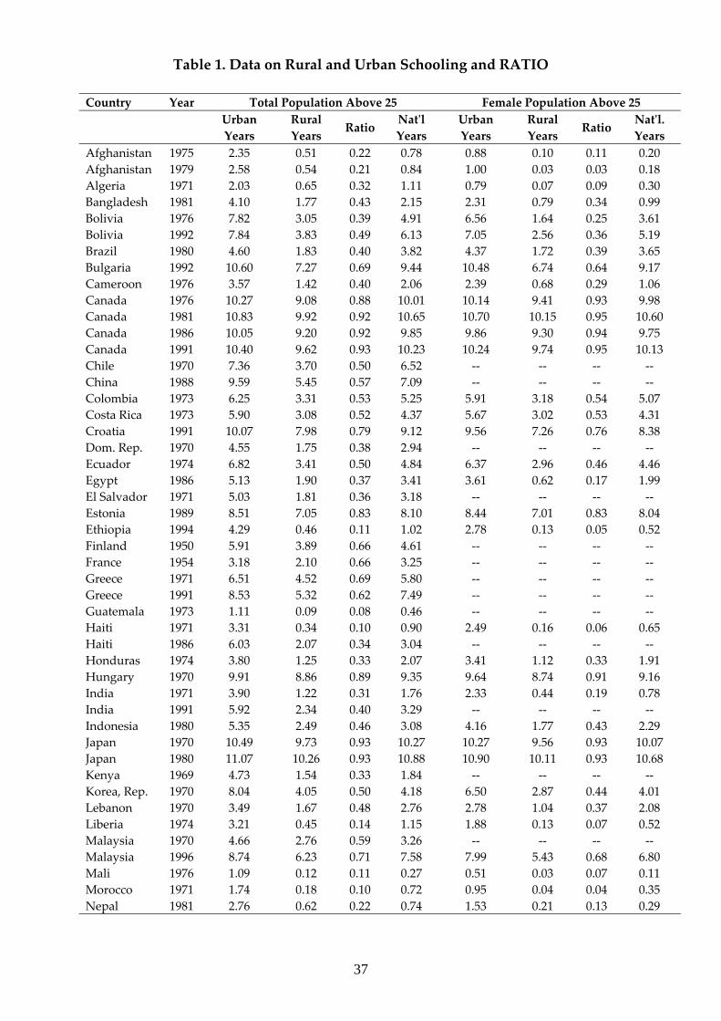
37
Table 1. Data on Rural and Urban Schooling and RATIO Country Year Total Population Above 25 Female Population Above 25
Urban Years
Rural Years
Ratio Natʹl Years
Urban Years
Rural Years
Ratio Natʹl. Years
Afghanistan 1975 2.35 0.51 0.22 0.78 0.88 0.10 0.11 0.20 Afghanistan 1979 2.58 0.54 0.21 0.84 1.00 0.03 0.03 0.18 Algeria 1971 2.03 0.65 0.32 1.11 0.79 0.07 0.09 0.30 Bangladesh 1981 4.10 1.77 0.43 2.15 2.31 0.79 0.34 0.99 Bolivia 1976 7.82 3.05 0.39 4.91 6.56 1.64 0.25 3.61 Bolivia 1992 7.84 3.83 0.49 6.13 7.05 2.56 0.36 5.19 Brazil 1980 4.60 1.83 0.40 3.82 4.37 1.72 0.39 3.65 Bulgaria 1992 10.60 7.27 0.69 9.44 10.48 6.74 0.64 9.17 Cameroon 1976 3.57 1.42 0.40 2.06 2.39 0.68 0.29 1.06 Canada 1976 10.27 9.08 0.88 10.01 10.14 9.41 0.93 9.98 Canada 1981 10.83 9.92 0.92 10.65 10.70 10.15 0.95 10.60 Canada 1986 10.05 9.20 0.92 9.85 9.86 9.30 0.94 9.75 Canada 1991 10.40 9.62 0.93 10.23 10.24 9.74 0.95 10.13 Chile 1970 7.36 3.70 0.50 6.52 ‐‐ ‐‐ ‐‐ ‐‐ China 1988 9.59 5.45 0.57 7.09 ‐‐ ‐‐ ‐‐ ‐‐ Colombia 1973 6.25 3.31 0.53 5.25 5.91 3.18 0.54 5.07 Costa Rica 1973 5.90 3.08 0.52 4.37 5.67 3.02 0.53 4.31 Croatia 1991 10.07 7.98 0.79 9.12 9.56 7.26 0.76 8.38 Dom. Rep. 1970 4.55 1.75 0.38 2.94 ‐‐ ‐‐ ‐‐ ‐‐ Ecuador 1974 6.82 3.41 0.50 4.84 6.37 2.96 0.46 4.46 Egypt 1986 5.13 1.90 0.37 3.41 3.61 0.62 0.17 1.99 El Salvador 1971 5.03 1.81 0.36 3.18 ‐‐ ‐‐ ‐‐ ‐‐ Estonia 1989 8.51 7.05 0.83 8.10 8.44 7.01 0.83 8.04 Ethiopia 1994 4.29 0.46 0.11 1.02 2.78 0.13 0.05 0.52 Finland 1950 5.91 3.89 0.66 4.61 ‐‐ ‐‐ ‐‐ ‐‐ France 1954 3.18 2.10 0.66 3.25 ‐‐ ‐‐ ‐‐ ‐‐ Greece 1971 6.51 4.52 0.69 5.80 ‐‐ ‐‐ ‐‐ ‐‐ Greece 1991 8.53 5.32 0.62 7.49 ‐‐ ‐‐ ‐‐ ‐‐ Guatemala 1973 1.11 0.09 0.08 0.46 ‐‐ ‐‐ ‐‐ ‐‐ Haiti 1971 3.31 0.34 0.10 0.90 2.49 0.16 0.06 0.65 Haiti 1986 6.03 2.07 0.34 3.04 ‐‐ ‐‐ ‐‐ ‐‐ Honduras 1974 3.80 1.25 0.33 2.07 3.41 1.12 0.33 1.91 Hungary 1970 9.91 8.86 0.89 9.35 9.64 8.74 0.91 9.16 India 1971 3.90 1.22 0.31 1.76 2.33 0.44 0.19 0.78 India 1991 5.92 2.34 0.40 3.29 ‐‐ ‐‐ ‐‐ ‐‐ Indonesia 1980 5.35 2.49 0.46 3.08 4.16 1.77 0.43 2.29 Japan 1970 10.49 9.73 0.93 10.27 10.27 9.56 0.93 10.07 Japan 1980 11.07 10.26 0.93 10.88 10.90 10.11 0.93 10.68 Kenya 1969 4.73 1.54 0.33 1.84 ‐‐ ‐‐ ‐‐ ‐‐ Korea, Rep. 1970 8.04 4.05 0.50 4.18 6.50 2.87 0.44 4.01 Lebanon 1970 3.49 1.67 0.48 2.76 2.78 1.04 0.37 2.08 Liberia 1974 3.21 0.45 0.14 1.15 1.88 0.13 0.07 0.52 Malaysia 1970 4.66 2.76 0.59 3.26 ‐‐ ‐‐ ‐‐ ‐‐ Malaysia 1996 8.74 6.23 0.71 7.58 7.99 5.43 0.68 6.80 Mali 1976 1.09 0.12 0.11 0.27 0.51 0.03 0.07 0.11 Morocco 1971 1.74 0.18 0.10 0.72 0.95 0.04 0.04 0.35 Nepal 1981 2.76 0.62 0.22 0.74 1.53 0.21 0.13 0.29
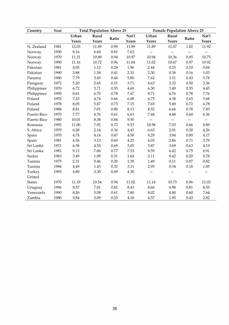
38
Country Year Total Population Above 25 Female Population Above 25
Urban Years
Rural Years Ratio Natʹl
Years Urban Years
Rural Years Ratio Natʹl
Years N. Zealand 1981 12.03 11.89 0.99 11.99 11.89 12.07 1.02 11.92 Norway 1950 8.16 6.60 0.81 7.63 ‐‐ ‐‐ ‐‐ ‐‐ Norway 1970 11.21 10.49 0.94 10.97 10.94 10.36 0.95 10.75 Norway 1990 11.16 10.72 0.96 11.04 11.02 10.67 0.97 10.92 Pakistan 1981 4.05 1.12 0.28 1.96 2.44 0.25 0.10 0.84 Pakistan 1990 3.88 1.58 0.41 2.31 2.30 0.38 0.16 1.03 Panama 1980 7.79 3.45 0.44 5.80 7.62 3.31 0.43 5.78 Paraguay 1972 5.20 2.65 0.51 3.71 4.63 2.33 0.50 3.36 Philippines 1970 6.72 3.71 0.55 4.69 6.30 3.49 0.55 4.45 Philippines 1995 8.61 6.70 0.78 7.67 8.71 6.76 0.78 7.76 Poland 1970 7.23 4.74 0.66 6.08 6.75 4.38 0.65 5.68 Poland 1978 8.05 5.87 0.73 7.15 7.65 5.49 0.72 6.78 Poland 1988 8.81 7.01 0.80 8.13 8.52 6.66 0.78 7.83 Puerto Rico 1970 7.77 4.76 0.61 6.63 7.44 4.48 0.60 6.36 Puerto Rico 1980 10.01 8.38 0.84 9.50 ‐‐ ‐‐ ‐‐ ‐‐ Romania 1992 11.00 7.92 0.72 9.53 10.58 7.03 0.66 8.89 S. Africa 1970 6.28 2.14 0.34 4.41 6.63 2.01 0.30 4.26 Spain 1970 4.74 4.14 0.87 4.58 4.29 3.84 0.89 4.17 Spain 1981 4.56 3.13 0.69 4.25 4.03 2.86 0.71 3.79 Sri Lanka 1971 6.58 4.55 0.69 5.05 5.87 3.69 0.63 4.19 Sri Lanka 1981 9.13 7.06 0.77 7.53 8.59 6.42 0.75 6.91 Sudan 1983 3.49 1.09 0.31 1.64 2.11 0.42 0.20 0.78 Tunisia 1975 2.31 0.46 0.20 1.59 1.49 0.11 0.07 0.82 Tunisia 1984 4.49 1.43 0.32 3.11 2.95 0.54 0.18 1.85 Turkey 1993 4.80 3.30 0.69 4.30 ‐‐ ‐‐ ‐‐ ‐‐ United States 1970 11.19 10.54 0.94 11.02 11.14 10.73 0.96 11.03 Uruguay 1996 8.57 7.01 0.82 8.43 8.66 6.98 0.81 8.55 Venezuela 1990 8.26 5.08 0.61 7.80 8.02 4.80 0.60 7.64 Zambia 1980 5.84 3.09 0.53 4.18 4.57 1.95 0.43 2.82

39
Table 2a. Descriptive Statistics (Total Population)
Table 2b. Descriptive Statistics (Total Pop. – Matched Years of National Schooling)
Table 2c. Descriptive Statistics (Female Population)
Table 2d. Descriptive Statistics (Male Population)
Table 2e. Developing vs. Developed Countries, Decade‐wise Means
Developing Countries Developed Countries # of
Obs. Rural Urban RATIO Nat’l (ours)
# of Obs. Rural Urban RATIO
Nat’l (ours)
1950s ‐‐ ‐‐ ‐‐ ‐‐ ‐‐ 3 4.20 5.75 0.71 5.16 1960s ‐‐ ‐‐ ‐‐ ‐‐ ‐‐ ‐‐ ‐‐ ‐‐ ‐‐ ‐‐ 1970s 31 2.41 4.95 0.41 3.38 6 8.08 9.07 0.88 8.78 1980s 16 3.49 6.23 0.49 4.58 5 8.88 9.71 0.89 9.52 1990s 12 4.98 7.72 0.60 6.39 3 8.56 10.03 0.84 9.59
Rural Years Urban Years RATIO Mean 4.23 6.53 0.55 Median 3.36 6.27 0.53 Std. Dev 3.23 2.89 0.25 Min. 0.10 1.09 0.09 Max. 11.89 12.03 0.99
National Years (ours)
National Years (Barro‐Lee,2001)
Mean 5.25 4.82 Median 4.59 4.27 Std. Dev 3.29 3.12 Min 0.27 0.26 Max. 11.99 11.43
Rural Years Urban Years RATIO National Years
(ours) Mean 4.01 5.99 0.51 4.94 Median 2.99 6.33 0.52 4.28 Std. Dev 3.65 3.42 0.32 3.70 Min. 0.03 0.51 0.03 0.11 Max. 12.07 11.89 1.02 11.92
Rural Years Urban Years RATIO National Years
(ours) Mean 4.86 7.31 0.59 5.89 Median 4.19 7,18 0.57 5.24 Std. Dev 3.30 2.74 0.25 3.31 Min. 0.22 1.70 0.12 0.44 Max. 11.74 12.19 0.96 12.07

40
Table 3. Summary Statistics for Explanatory Variables Variable Mean Median Max Min St. Dev. Obs. Agr. ValueAdded/worker ($) 5,449 1,917 32,470 137 7,432 59 NonAgr. VA/worker ($) 13,641 6,600 64,257 628 15,182 58 Relative Income 0.38 0.29 2.80 0.03 0.38 58 Real Income/capita ($) 5,273 1,616 30,493 95 7,175 70 Education Expend. (% of GDP) 3.62 3.39 7.54 1.14 1.65 66 M2/GDP (%) 34.75 30.35 89.05 8.13 18.56 60 Industry VA/Total VA (%) 31.12 30.89 52.30 10.43 9.60 63 Services VA/Total VA (%) 49.07 49.34 73.45 26.50 10.17 63 Agr. VA/Total VA (%) 19.80 18.62 61.07 2.26 14.17 63 Land Gini Index 64.03 62.72 93.31 33.85 15.90 54 Hectares of arable land/person 0.37 0.27 1.87 0.02 0.39 74 Migration (%) 12.55 12.34 36.98 ‐2.35 8.37 72 Agr. Deflator/NonAgr. Def. 1.18 1.07 2.94 0.59 0.40 59 Female Teachers (% of all) 51.83 56.28 92.00 8.00 24.17 49 Doctors (per 1,000 people) 0.95 0.50 4.78 0.02 1.05 64 Fertilizer Cons. (kg/hectare) 113.18 76.94 695.53 1.97 123.44 72 Pupil/Teacher in Pri. Educ. 30.60 30.98 56.87 12.53 10.05 61 Phone lines (per 1,000 people) 108.30 32.03 578.70 0.60 152.36 68 Tractors (per 100 hectares) 2.25 0.86 31.51 0.01 4.51 72 Life Expectancy (years) 63.27 65.67 77.65 39.60 10.11 75 Nat. Pop. Density (people) 97.57 52.64 785.28 2.58 125.16 74 Rural Pop. Density (people) 332.46 176.56 1558.77 13.00 345.72 74 Rural Births (per 1,000 people) 28.75 30.80 64.00 2.50 11.95 59 Rural Deaths (per 1,000 people) 10.86 9.70 50.40 1.20 6.89 56 Rural Pop./Tot. Pop. (%) 51.72 49.48 92.99 8.91 20.80 75 Urban Births (per 1,000 people) 25.06 21.30 59.30 7.80 12.99 59 Urban Deaths (per 1,000 people) 9.35 8.50 42.80 3.00 5.53 55 Urban Pop./Tot. Pop. (%) 48.28 50.52 91.09 7.01 20.80 75 Relative Birth Rate 1.28 1.20 3.04 0.21 0.55 59 Relative Death Rate 1.23 1.24 2.43 0.27 0.46 44 Relative Population 1.79 0.98 13.24 0.10 2.15 75 Ethnic Frac. Index 0.40 0.42 0.91 0.00 0.27 73 Island Dummy 0.17 0 1 0 0.38 75 Landlocked Dummy 0.11 0 1 0 0.31 75 Tropical Dummy 0.40 0 1 0 0.49 75 Latitude (absolute value) 28.36 30.00 60.21 0.51 16.28 75 British Legal Sys. Dummy 0.28 0 1 0 0.45 75 French Legal Sys. Dummy 0.51 1 1 0 0.50 75 German Legal Sys. Dummy 0.04 0 1 0 0.20 75 Scandin. Legal Sys. Dummy 0.05 0 1 0 0.23 75 Socialist Legal Sys. Dummy 0.12 0 1 0 0.33 75 Political Rights Index 3.79 4.27 7.00 1.00 2.00 68 Civil Liberties Index 3.78 4.00 6.80 1.00 1.68 68 Colony Dummy 0.67 1 1 0 0.47 75 No. of Revolutions (5‐year avg.) 0.17 0.00 1.25 0.00 0.27 66 Post‐war Indep. Dummy 0.39 0 1 0 0.49 75 No. of Assassin. (5‐year avg.) 0.28 0.00 3.25 0.00 0.65 66 Catholic (% of total population) 39.12 26.20 96.90 0.00 40.42 75 Confucian (% of total pop.) 4.57 0.00 98.50 0.00 20.03 75 Protestant (% of total pop.) 12.35 1.90 97.80 0.00 23.81 75 Girl‐boy ratio (%) 82.20 91.22 103.29 16.80 20.18 57
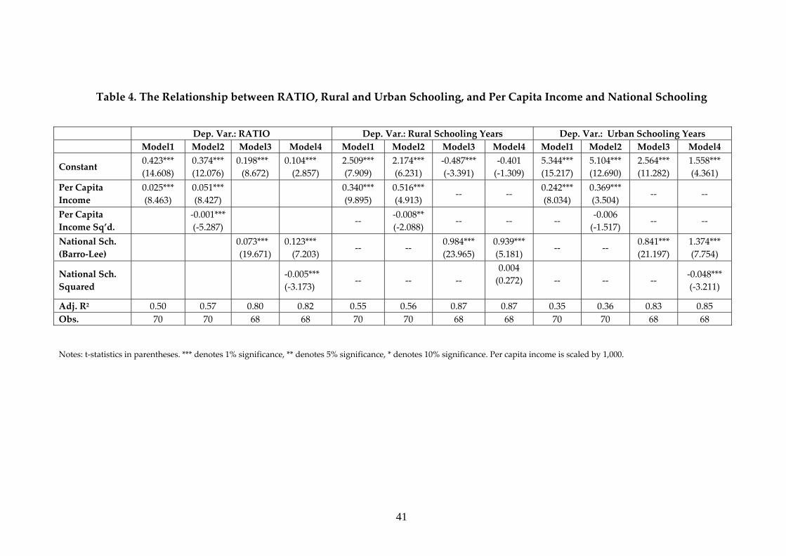
41
Table 4. The Relationship between RATIO, Rural and Urban Schooling, and Per Capita Income and National Schooling
Dep. Var.: RATIO Dep. Var.: Rural Schooling Years Dep. Var.: Urban Schooling Years Model1 Model2 Model3 Model4 Model1 Model2 Model3 Model4 Model1 Model2 Model3 Model4
Constant 0.423*** (14.608)
0.374*** (12.076)
0.198*** (8.672)
0.104*** (2.857)
2.509*** (7.909)
2.174*** (6.231)
‐0.487*** (‐3.391)
‐0.401 (‐1.309)
5.344*** (15.217)
5.104*** (12.690)
2.564*** (11.282)
1.558*** (4.361)
Per Capita Income
0.025*** (8.463)
0.051*** (8.427)
0.340*** (9.895)
0.516*** (4.913) ‐‐ ‐‐
0.242*** (8.034)
0.369*** (3.504) ‐‐ ‐‐
Per Capita Income Sq’d.
‐0.001*** (‐5.287) ‐‐
‐0.008** (‐2.088) ‐‐ ‐‐ ‐‐
‐0.006 (‐1.517) ‐‐ ‐‐
National Sch. (Barro‐Lee)
0.073*** (19.671)
0.123*** (7.203) ‐‐ ‐‐
0.984*** (23.965)
0.939*** (5.181) ‐‐ ‐‐
0.841*** (21.197)
1.374*** (7.754)
National Sch. Squared
‐0.005*** (‐3.173) ‐‐ ‐‐ ‐‐
0.004 (0.272)
‐‐ ‐‐ ‐‐ ‐0.048*** (‐3.211)
Adj. R2 0.50 0.57 0.80 0.82 0.55 0.56 0.87 0.87 0.35 0.36 0.83 0.85 Obs. 70 70 68 68 70 70 68 68 70 70 68 68 Notes: t‐statistics in parentheses. *** denotes 1% significance, ** denotes 5% significance, * denotes 10% significance. Per capita income is scaled by 1,000.
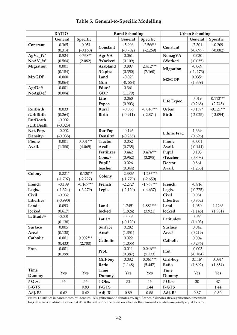
42
Table 5. General‐to‐Specific Modelling
RATIO Rural Schooling Urban Schooling General Specific General Specific General Specific Constant 0.365
(0.314) ‐0.051 (‐0.168)
Constant ‐5.906 (‐0.702)
‐2.566** (‐2.269)
Constant ‐7.301 (‐0.697)
‐0.209 (‐0.082)
AgVa_W/ NoAV_W
0.524 (0.564)
0.768** (2.082)
Agr.VA /Worker§
0.061 (0.109)
NonagVA /Worker§
‐0.030 (‐0.055)
Migration 0.001 (0.184)
Arabland/Capita
0.807 (0.350)
2.412*** (7.160)
Migration ‐0.069 (‐1. 173)
M2/GDP 0.000 (0.064)
Land Gini
‐0.029 (‐0. 554)
M2/GDP 0.035* (1.889)
AgrDef/ NoAgDef
0.001 (0.004)
Educ./GDP
0.361 (1.179)
Life Expec.
0.060 (0.903)
Life Expec. 0.019 (0.268)
0.113*** (2.745)
RurBirth /UrbBirth
0.033 (0.264)
Rural Birth
‐0.036 (‐0.911)
‐0.046*** (‐2.874)
Urban Birth
‐0.139* (‐2.025)
‐0.121*** (‐3.094)
RurDeath /UrbDeath
‐0.002 (‐0.023)
Nat. Pop. Density§
‐0.002 (‐0.038)
Rur Pop Density§
‐0.193 (‐0.255)
Ethnic Frac. 1.669 (0.696)
Phone Avail.
0.001 (1.380)
0.001*** (4.065)
Tractor Avail.
0.052 (0.735)
Phone Avail.
‐0.001 (‐0.144)
Fertilizer Cons. §
0.442 (0.962)
0.474*** (3.295)
Pupil /Teacher
0.103 (0.808)
Pupil/teacher
0.026 (0.344)
Doctor Avail.
0.861 (1.235)
Colony ‐0.221* (‐1.797)
‐0.120** (‐2.227)
Colony ‐2.386* (‐1.779)
‐1.236*** (‐2.650)
French Legis.
‐0.189 (‐1.324)
‐0.167*** (‐3.279)
French Legis.
‐2.272* (‐2.120)
‐1.768*** (‐4.637)
French Legis.
‐0.816 (‐0.775)
Civil Liberties
‐0.032 (‐0.990)
Civil Liberties
0.081 (0.352)
Land‐ locked
0.093 (0.617)
Land‐locked
1.745* (1.824)
1.881*** (3.921)
Land‐ locked
1.050 (1.146)
1.126* (1.981)
Latitude§§ ‐0.001 (0.138)
Latit.§§ ‐0.005 (‐0.120)
Latitude§§ 0.064 (1.403)
Surface Area§
0.005 (0.138)
SurfaceArea§
0.282 (1.351)
Surface Area§
0.042 (0.219)
Catholic 0.001 (0.433)
0.002*** (2.700)
Catholic 0.022 (1.055)
Catholic 0.004 (0.276)
Prot. 0.001 (0.399)
Prot. 0.011 (0.387)
0.046*** (5.133)
Prot. ‐0.003 (‐0.184)
Girl‐boyRatio
0.032 (1.148)
0.061*** (5.447)
Girl‐boy Ratio
0.116* (1.892)
0.031* (1.854)
Time Dummy Yes Yes
Time Dummy Yes Yes
Time Dummy Yes Yes
# Obs. 36 56 # Obs. 32 46 # Obs. 30 47 F‐GTS 0.83 F‐GTS 1.44 F‐GTS 1.44 Adj. R2 0.62 0.62 Adj. R2 0.89 0.88 Adj. R2 0.87 0.80 Notes: t‐statistics in parentheses. *** denotes 1% significance, ** denotes 5% significance, * denotes 10% significance. § means in logs. §§ means in absolute value. F‐GTS is the statistic of the F‐test on whether the removed variables are jointly equal to zero.

43
Table 6. Cross-country Determinants of RATIO
Notes: t‐statistics in parentheses. *** denotes 1% significance, ** 5% significance, * 10% significance. § means in logs. §§ means in absolute value. White heteroskedasticity‐consistent standard errors. Added Var. denotes that the relevant model is augmented over the form in Equation (6) to treat the omitted variables problem. Time dummies included in the regressions but not reported to save space; a great majority of them are insignificant and all of them are jointly insigificant in the respective models. LM‐ test ‐ χ2 is the chi‐squared test statistic of the LM test, and LM test–F. Stat. is the F statistic of the same test. See the text for the difference. Reset F.stat . is the test statistic of the omitted variables test. C+C+P is the sum of the shares of confucian, catholic and protestant populations in total population.
Ratio1 (Credit Cons.)
Ratio2 (Labor Market)
Ratio3 (Migration)
Ratio4 (Inv. Riskiness)
Ratio5 (Infrast. Avail.)
Constant 0.514*** (3.706)
‐0.746** (‐2.572)
0.588*** (4.820)
‐0.095 (‐0.292)
1.228*** (5.332)
Economic Var. M2/GDP
0.004*** (2.681)
AgVA_W/NoAgV_W
1.278*** (3.847) Migrat.
0.007** (2.214)
Educ.Exp./ GDP
0.035* (1.701)
Demog. Var.
NatPop Density.§
‐0.043** (‐2.158)
RurBirth /UrbBirth
0.124*** (2.991)
Rurdeath /UrbDeath
‐0.129* (‐1.802)
RurPop /UrbPop
‐0.037*** (‐3.603)
Infrast. Var.
Pupil /Teach.
‐0.006** (‐2.564)
Doctor Avail.
0.089* (1.815)
Phone Avail.
0.001*** (3.559)
Political Var Colony
‐0.136** (‐2.080)
French Legisl.
‐0.131** (‐2.371)
Pol. Rights
‐0.021 (‐1.552) British Leg.
0.321*** (4.861)
No. of Revol.
‐0.121** (‐2.208)
Geog. Var.
Land‐ locked
‐0.188*** (‐3.144) Island
0.289*** (5.422) Latit.§§
0.003* (1.965)
Surface Area§
‐0.032** (‐2.246)
Cultural Var.
C+C+P
0.002*** (2.984)
C+C+P
0.001** (2.032) Conf.
0.002*** (4.005) Conf.
0.002*** (4.367)
Added Var.
Sub‐sah. Africa
‐0.077 (‐0.675)
AgVA_W /NAVA_W
0.619* (1.659)
Pupil /Teacher
‐0.009*** (‐2.979)
Added Var. Confucian
0.001* (1.752)
British Legis.
0.114** (2.367)
Added Var.
Postwar Independ.
‐0.204** (‐2.617)
Adj. R2 0.37 0.70 0.50 0.68 0.61 A/S ‐0.22/‐0.06 ‐0.87/‐0.54 ‐0.61/‐0.32 ‐0.61/‐0.17 ‐0.68/‐0.40 LM ‐ χ2 17.99*** 24.97*** 25.75*** 11.56*** 9.76*** LM–F. stat 7.93*** 16.30*** 20.61*** 9.99*** 5.26*** Reset F.st 2.30 0.26 0.78 1.79 0.57 Obs. 60 45 58 36 48
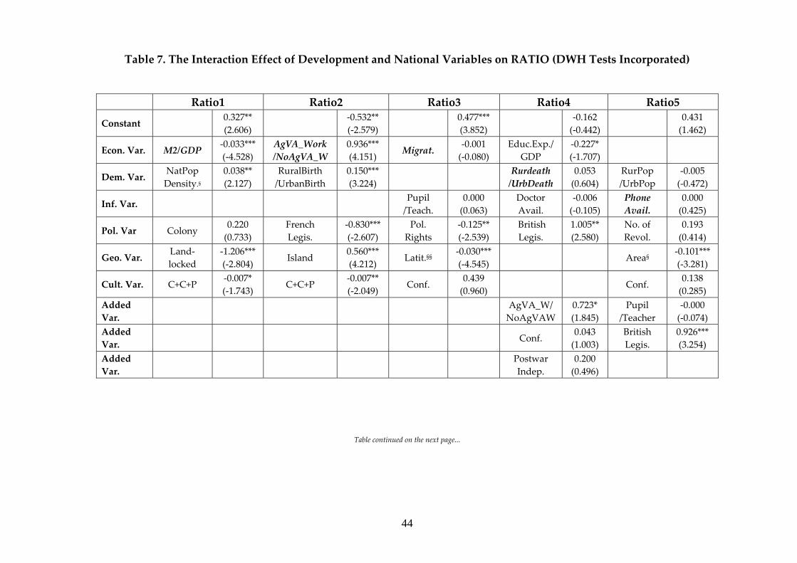
44
Table 7. The Interaction Effect of Development and National Variables on RATIO (DWH Tests Incorporated)
Table continued on the next page...
Ratio1 Ratio2 Ratio3 Ratio4 Ratio5
Constant 0.327** (2.606)
‐0.532** (‐2.579)
0.477*** (3.852)
‐0.162 (‐0.442)
0.431 (1.462)
Econ. Var. M2/GDP ‐0.033*** (‐4.528)
AgVA_Work /NoAgVA_W
0.936*** (4.151) Migrat.
‐0.001 (‐0.080)
Educ.Exp./ GDP
‐0.227* (‐1.707)
Dem. Var. NatPop Density.§
0.038** (2.127)
RuralBirth /UrbanBirth
0.150*** (3.224)
Rurdeath /UrbDeath
0.053 (0.604)
RurPop /UrbPop
‐0.005 (‐0.472)
Inf. Var. Pupil /Teach.
0.000 (0.063)
Doctor Avail.
‐0.006 (‐0.105)
Phone Avail.
0.000 (0.425)
Pol. Var Colony 0.220 (0.733)
French Legis.
‐0.830*** (‐2.607)
Pol. Rights
‐0.125** (‐2.539)
British Legis.
1.005** (2.580)
No. of Revol.
0.193 (0.414)
Geo. Var. Land‐ locked
‐1.206*** (‐2.804) Island
0.560*** (4.212) Latit.§§
‐0.030*** (‐4.545) Area§
‐0.101*** (‐3.281)
Cult. Var. C+C+P ‐0.007* (‐1.743) C+C+P
‐0.007** (‐2.049) Conf.
0.439 (0.960) Conf.
0.138 (0.285)
Added Var.
AgVA_W/ NoAgVAW
0.723* (1.845)
Pupil /Teacher
‐0.000 (‐0.074)
Added Var. Conf.
0.043 (1.003)
British Legis.
0.926*** (3.254)
Added Var.
Postwar Indep.
0.200 (0.496)
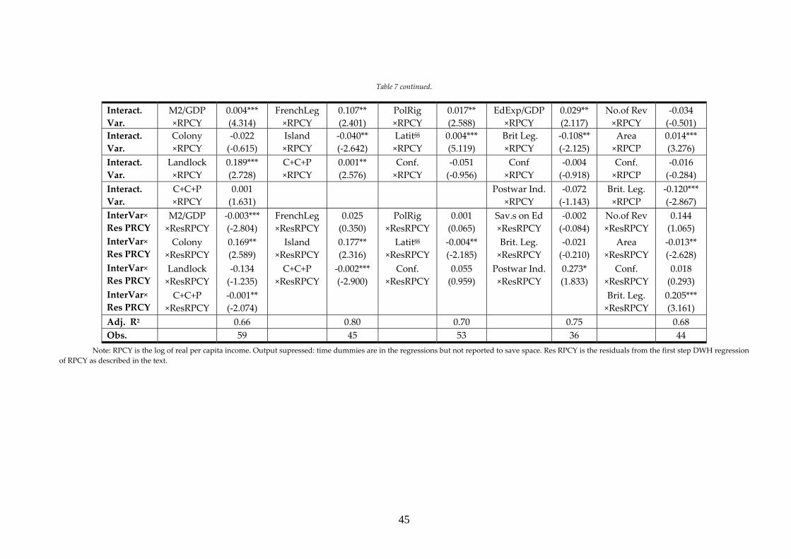
45
Table 7 continued.
Note: RPCY is the log of real per capita income. Output supressed: time dummies are in the regressions but not reported to save space. Res RPCY is the residuals from the first step DWH regression of RPCY as described in the text.
Interact.Var.
M2/GDP ×RPCY
0.004*** (4.314)
FrenchLeg ×RPCY
0.107** (2.401)
PolRig ×RPCY
0.017** (2.588)
EdExp/GDP ×RPCY
0.029** (2.117)
No.of Rev ×RPCY
‐0.034 (‐0.501)
Interact. Var.
Colony ×RPCY
‐0.022 (‐0.615)
Island ×RPCY
‐0.040** (‐2.642)
Latit§§ ×RPCY
0.004*** (5.119)
Brit Leg. ×RPCY
‐0.108** (‐2.125)
Area ×RPCP
0.014*** (3.276)
Interact. Var.
Landlock ×RPCY
0.189*** (2.728)
C+C+P ×RPCY
0.001** (2.576)
Conf. ×RPCY
‐0.051 (‐0.956)
Conf ×RPCY
‐0.004 (‐0.918)
Conf. ×RPCP
‐0.016 (‐0.284)
Interact. Var.
C+C+P ×RPCY
0.001 (1.631)
Postwar Ind.×RPCY
‐0.072 (‐1.143)
Brit. Leg. ×RPCP
‐0.120*** (‐2.867)
InterVar×Res PRCY
M2/GDP ×ResRPCY
‐0.003*** (‐2.804)
FrenchLeg ×ResRPCY
0.025 (0.350)
PolRig ×ResRPCY
0.001 (0.065)
Sav.s on Ed ×ResRPCY
‐0.002 (‐0.084)
No.of Rev ×ResRPCY
0.144 (1.065)
InterVar×Res PRCY
Colony ×ResRPCY
0.169** (2.589)
Island ×ResRPCY
0.177** (2.316)
Latit§§ ×ResRPCY
‐0.004** (‐2.185)
Brit. Leg. ×ResRPCY
‐0.021 (‐0.210)
Area ×ResRPCY
‐0.013** (‐2.628)
InterVar×Res PRCY
Landlock ×ResRPCY
‐0.134 (‐1.235)
C+C+P ×ResRPCY
‐0.002*** (‐2.900)
Conf. ×ResRPCY
0.055 (0.959)
Postwar Ind.×ResRPCY
0.273* (1.833)
Conf. ×ResRPCY
0.018 (0.293)
InterVar×Res PRCY
C+C+P ×ResRPCY
‐0.001** (‐2.074)
Brit. Leg. ×ResRPCY
0.205*** (3.161)
Adj. R2 0.66 0.80 0.70 0.75 0.68 Obs. 59 45 53 36 44
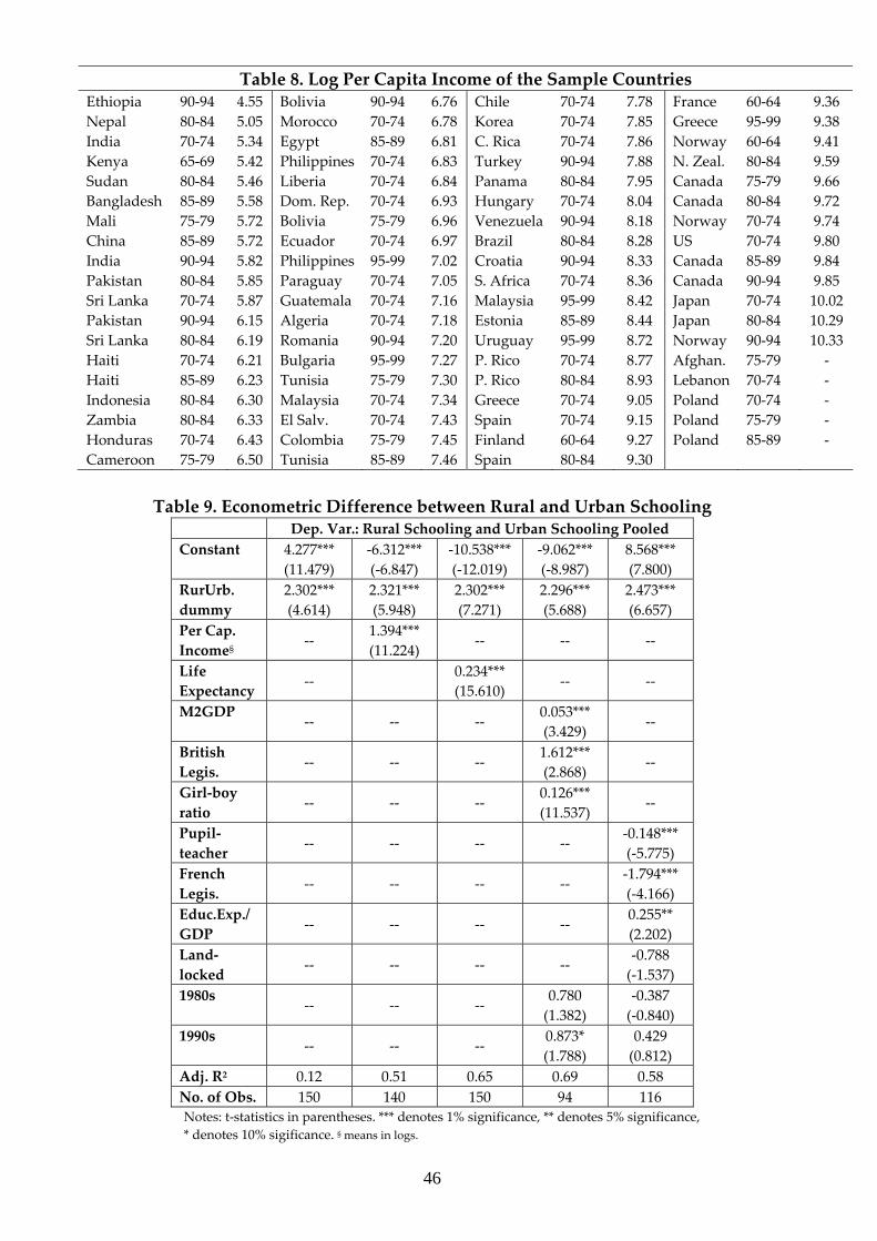
46
Table 8. Log Per Capita Income of the Sample Countries Ethiopia 90‐94 4.55 Bolivia 90‐94 6.76 Chile 70‐74 7.78 France 60‐64 9.36 Nepal 80‐84 5.05 Morocco 70‐74 6.78 Korea 70‐74 7.85 Greece 95‐99 9.38 India 70‐74 5.34 Egypt 85‐89 6.81 C. Rica 70‐74 7.86 Norway 60‐64 9.41 Kenya 65‐69 5.42 Philippines 70‐74 6.83 Turkey 90‐94 7.88 N. Zeal. 80‐84 9.59 Sudan 80‐84 5.46 Liberia 70‐74 6.84 Panama 80‐84 7.95 Canada 75‐79 9.66 Bangladesh 85‐89 5.58 Dom. Rep. 70‐74 6.93 Hungary 70‐74 8.04 Canada 80‐84 9.72 Mali 75‐79 5.72 Bolivia 75‐79 6.96 Venezuela 90‐94 8.18 Norway 70‐74 9.74 China 85‐89 5.72 Ecuador 70‐74 6.97 Brazil 80‐84 8.28 US 70‐74 9.80 India 90‐94 5.82 Philippines 95‐99 7.02 Croatia 90‐94 8.33 Canada 85‐89 9.84 Pakistan 80‐84 5.85 Paraguay 70‐74 7.05 S. Africa 70‐74 8.36 Canada 90‐94 9.85 Sri Lanka 70‐74 5.87 Guatemala 70‐74 7.16 Malaysia 95‐99 8.42 Japan 70‐74 10.02 Pakistan 90‐94 6.15 Algeria 70‐74 7.18 Estonia 85‐89 8.44 Japan 80‐84 10.29 Sri Lanka 80‐84 6.19 Romania 90‐94 7.20 Uruguay 95‐99 8.72 Norway 90‐94 10.33 Haiti 70‐74 6.21 Bulgaria 95‐99 7.27 P. Rico 70‐74 8.77 Afghan. 75‐79 ‐ Haiti 85‐89 6.23 Tunisia 75‐79 7.30 P. Rico 80‐84 8.93 Lebanon 70‐74 ‐ Indonesia 80‐84 6.30 Malaysia 70‐74 7.34 Greece 70‐74 9.05 Poland 70‐74 ‐ Zambia 80‐84 6.33 El Salv. 70‐74 7.43 Spain 70‐74 9.15 Poland 75‐79 ‐ Honduras 70‐74 6.43 Colombia 75‐79 7.45 Finland 60‐64 9.27 Poland 85‐89 ‐ Cameroon 75‐79 6.50 Tunisia 85‐89 7.46 Spain 80‐84 9.30
Table 9. Econometric Difference between Rural and Urban Schooling
Dep. Var.: Rural Schooling and Urban Schooling Pooled Constant 4.277***
(11.479) ‐6.312*** (‐6.847)
‐10.538*** (‐12.019)
‐9.062*** (‐8.987)
8.568*** (7.800)
RurUrb. dummy
2.302*** (4.614)
2.321*** (5.948)
2.302*** (7.271)
2.296*** (5.688)
2.473*** (6.657)
Per Cap. Income§ ‐‐ 1.394***
(11.224) ‐‐ ‐‐ ‐‐
Life Expectancy ‐‐ 0.234***
(15.610) ‐‐ ‐‐
M2GDP ‐‐ ‐‐ ‐‐ 0.053***
(3.429) ‐‐
British Legis. ‐‐ ‐‐ ‐‐ 1.612***
(2.868) ‐‐
Girl‐boy ratio ‐‐ ‐‐ ‐‐ 0.126***
(11.537) ‐‐
Pupil‐teacher ‐‐ ‐‐ ‐‐ ‐‐ ‐0.148***
(‐5.775) French Legis. ‐‐ ‐‐ ‐‐ ‐‐ ‐1.794***
(‐4.166) Educ.Exp./ GDP ‐‐ ‐‐ ‐‐ ‐‐ 0.255**
(2.202) Land‐locked ‐‐ ‐‐ ‐‐ ‐‐ ‐0.788
(‐1.537) 1980s
‐‐ ‐‐ ‐‐ 0.780 (1.382)
‐0.387 (‐0.840)
1990s ‐‐ ‐‐ ‐‐ 0.873*
(1.788) 0.429 (0.812)
Adj. R2 0.12 0.51 0.65 0.69 0.58 No. of Obs. 150 140 150 94 116 Notes: t‐statistics in parentheses. *** denotes 1% significance, ** denotes 5% significance, * denotes 10% sigificance. § means in logs.

47
Table 10a. Cross‐country Determinants of Levels of Rural Schooling Years ‐ OLS Notes: t‐statistics in parentheses. *** denotes 1% significance, ** 5% significance, * 10% significance. § in logs. §§ in absolute value. White heteroskedasticity‐consistent standard errors. Added Var. denotes that the relevant model is augmented to treat the omitted variables case. ResLife Expec. is the residual of life expectancy from the first‐step DWH regressions (using theoretical instruments) and is in Rural1 to obtain consistent coefficients. See Appendix B for details. Time dummies are in the regressions but not reported to save space; all of them are jointly insigificant in the respective models. LM statistics test the variable additions over and above the STG models in Equation (6) for which the additions are tested over and above Equation (5). Reset F.‐st. is for the omitted variables test.
Rural 1 (Infrast. Avail.)
Rural 2 (Labor Market)
Rural 3 (Credit Cons.)
Rural 4 (Labor Market)
Rural 5 (Inv. Riskiness)
Constant† ‐3.674 (‐1.130)
‐0.964 (0.477)
8.215*** (4.500)
8.088*** (4.151)
‐7.219 (‐1.651)
Economic Var.
Arland /capita
1.789*** (3.466)
Agr.VA /work.§
1.028*** (7.077)
Land Gini
‐0.057*** (‐3.758)
Educ.Exp./ GDP
0.432* (1.996)
AgrDef/ GDPDef
2.864 (1.664)
Demog. Var.
Life Expec.
0.094* (1.740)
RuralPop Density§
‐1.653*** (‐7.342)
Rural birth
‐0.05*** (‐2.243)
Rural death
‐0.113** (‐2.574)
Infrast. Var.
Tractor Avail.
0.207** (2.480)
Pupil /teach
‐0.069*** (‐2.873)
Fertilizer Cons. §
0.729*** (4.003)
Pupil /teacher
‐0.137*** (‐4.117)
Tractor Avail.
0.183* (1.744)
Political Var
British Legis.
1.381** (2.260)
French Legis.
‐1.581*** (‐3.832)
No of. Assassin.
‐0.558*** (‐2.838)
French Legis.
‐2.200*** (‐3.010)
Colony dummy
‐2.672* (‐1.786)
Geog. Var.
Land‐ locked
1.227 (1.489) Island
1.625*** (2.948)
Arable /tot. land
‐0.008 (‐0.350)
Surface Area§
0.815** (2.550)
Cultural Var.
Cath.+ Prot.
0.021*** (4.434)
C+C+P
0.018** (2.332)
Added Var.
Germ. Leg.
1.869 (1.370)
Tractor Avail.
0.056** (2.259)
Tractor Avail.
0.166** (2.111)
Female Teacher
0.022* (2.008)
Added Var.
ResLife Expec.
0.146*** (3.104)
Land Gini
‐0.053*** (3.753) Colony
1.338* (1.984)
German Legis.
3.585*** (3.969)
Added Var. Island
2.919*** (2.864)
Adj. R2 0.75 0.88 0.72 0.81 0.35 A/S 4.00/4.37 3.06/3.08 4.19/4.61 3.71/4.15 5.14/5.46 LM ‐ χ2 48.23*** 14.58*** 18.70*** 12.96*** 17.87*** LM ‐ F. St. 6.86*** 10.67*** 7.16*** 8.85*** 7.00*** Reset‐F.st. 0.01 0.78 2.59 2.78 0.98 Obs. 54 40 50 36 44
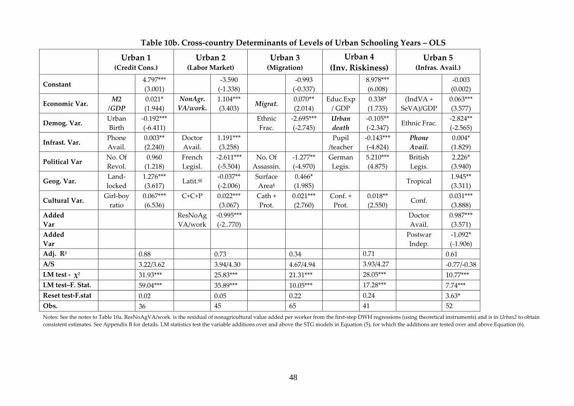
48
Table 10b. Cross‐country Determinants of Levels of Urban Schooling Years – OLS
Notes: See the notes to Table 10a. ResNoAgVA/work. is the residual of nonagricultural value added per worker from the first‐step DWH regressions (using theoretical instruments) and is in Urban2 to obtain consistent estimates. See Appendix B for details. LM statistics test the variable additions over and above the STG models in Equation (5), for which the additions are tested over and above Equation (6).
Urban 1 (Credit Cons.)
Urban 2 (Labor Market)
Urban 3 (Migration)
Urban 4 (Inv. Riskiness)
Urban 5 (Infras. Avail.)
Constant 4.797*** (3.001)
‐3.590 (‐1.338)
‐0.993 (‐0.337)
8.978*** (6.008)
‐0.003 (0.002)
Economic Var. M2 /GDP
0.021* (1.944)
NonAgr.VA/work.
1.104*** (3.403) Migrat.
0.070** (2.014)
Educ.Exp/ GDP
0.338* (1.735)
(IndVA + SeVA)/GDP
0.063*** (3.577)
Demog. Var. Urban Birth
‐0.192*** (‐6.411)
Ethnic Frac.
‐2.695*** (‐2.745)
Urban death
‐0.105** (‐2.347) Ethnic Frac.
‐2.824** (‐2.565)
Infrast. Var. Phone Avail.
0.003** (2.240)
Doctor Avail.
1.191*** (3.258)
Pupil /teacher
‐0.143*** (‐4.824)
Phone Avail.
0.004* (1.829)
Political Var No. Of Revol.
0.960 (1.218)
French Legisl.
‐2.611*** (‐5.504)
No. Of Assassin.
‐1.277** (‐4.970)
German Legis.
5.210*** (4.875)
British Legis.
2.226* (3.940)
Geog. Var. Land‐ locked
1.276*** (3.617) Latit.§§
‐0.037** (‐2.006)
Surface Area§
0.466* (1.985) Tropical
1.945** (3.311)
Cultural Var. Girl‐boy ratio
0.067*** (6.536)
C+C+P
0.022*** (3.067)
Cath + Prot.
0.021*** (2.760)
Conf. + Prot.
0.018** (2.550) Conf.
0.031*** (3.888)
Added Var
ResNoAgVA/work
‐0.995*** (‐2..770)
Doctor Avail.
0.987*** (3.571)
Added Var
Postwar Indep.
‐1.092* (‐1.906)
Adj. R2 0.88 0.73 0.34 0.71 0.61 A/S 3.22/3.62 3.94/4.30 4.67/4.94 3.93/4.27 ‐0.77/‐0.38 LM test ‐ χ2 31.93*** 25.83*** 21.31*** 28.05*** 10.77*** LM test–F. Stat. 59.04*** 35.89*** 10.05*** 17.28*** 7.74*** Reset test‐F.stat 0.02 0.05 0.22 0.24 3.63* Obs. 36 45 65 41 52

49
Table 11a. Cross‐country Determinants of Rural Educational Attainment – Cross‐Dependent Variable Validation Notes: t‐statistics in parantheses. *** denotes 1% significance, ** 5% significance, * 10% significance. § means in logs. §§ means in absolute value. White heteroskedasticity‐consistent standard errors.
† means the dependent variable is Urban Educational Attainment. OLS regressions.
Rural 1† Rural 2† Rural 3† Rural 4† Rural 5†
Constant ‐6.836*** (‐4.475)
4.646 (1.608)
7.464*** (3.327)
8.978*** (4.645)
‐2.199 (‐0.626)
Economic Var.
Arland/capita
0.809* (1.843)
Agr.VA/work.§
0.729*** (2.869)
Land Gini
‐0.045** (‐2.632)
Savings on Educ.
0.255 (1.149)
AgrDef /GDPDef
0.063*** (3.577)
Demog. Var.
Life Expec.
0.193*** (7.325)
RuralPop Density§
‐1.024*** (‐4.682)
Rural birth
‐0.083*** (‐5.042)
Rural Death
‐0.154*** (‐4.602)
Infrast. Var.
Tract. /hect’e
0.035 (0.064)
Pupil /teac’r.
‐0.063 (‐1.351)
Fertilizer /hectare §
0.605** (2.223)
Pupil /teacher
‐0.068* (‐1.917)
Tractor /hectare
0.097 (1.294)
Political Var
British Legis.
0.790** (1.555)
French Legisl.
‐1.291*** (‐3.182)
No of. Assassin.
‐0.784*** (‐2.224)
French Legis.
‐1.977*** (‐3.314)
Colony ‐2.501* (‐1.916)
Geog. Var.
Land locked
1.269** (1.612) Island
1.426*** (2.780)
Arabland /tot. land
‐0.019 (‐1.081)
Area 0.619* (2.165)
Cultural Var.
Cath+ Prot
0.022*** (3.700)
Conf.+Cath+ Prot.
0.024** (2.925)
1980s 0.307 (0.548)
0.132 (0.218)
0.561 (0.944)
1.789 (1.671)
1990s 1.133* (1.795)
1.262** (2.069)
0.715 (1.282)
1.778* (1.878)
Added Var.
Germ. Leg.
2.588* (3.557)
Tractor/hect’e.
0.036 (1.327)
Tractor /hectare
0.103** (1.613)
FemTeac./TotTeac.
0.039*** (2.749)
Added Var.
Land gini
‐0.045** (‐2.275) Colony
1.614** (2.103)
German Legis.
2.203** (2.299)
Added Var. Island
2.227** (2.550)
Adj. R2 0.60 0.69 0.58 0.80 0.37 Obs. 71 40 50 36 44
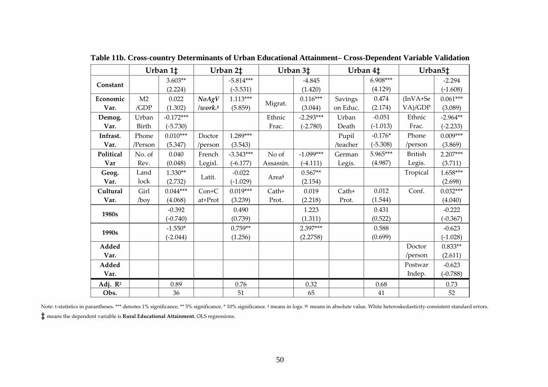
50
Table 11b. Cross-country Determinants of Urban Educational Attainment– Cross-Dependent Variable Validation Note: t‐statistics in parantheses. *** denotes 1% significance, ** 5% significance, * 10% significance. § means in logs. §§ means in absolute value. White heteroskedasticity‐consistent standard errors. ‡ means the dependent variable is Rural Educational Attainment. OLS regressions.
Urban 1‡ Urban 2‡ Urban 3‡ Urban 4‡ Urban5‡
Constant 3.603** (2.224)
‐5.814*** (‐3.531)
‐4.845 (1.420)
6.908*** (4.129)
‐2.294 (‐1.608)
Economic Var.
M2 /GDP
0.022 (1.302)
NoAgV/work.§
1.113*** (5.859) Migrat.
0.116*** (3.044)
Savings on Educ.
0.474 (2.174)
(InVA+SeVA)/GDP
0.061*** (3.089)
Demog. Var.
Urban Birth
‐0.172*** (‐5.730)
Ethnic Frac.
‐2.293*** (‐2.780)
Urban Death
‐0.051 (‐1.013)
Ethnic Frac.
‐2.964** (‐2.233)
Infrast. Var.
Phone /Person
0.010*** (5.347)
Doctor /person
1.289*** (3.543)
Pupil /teacher
‐0.176* (‐5.308)
Phone /person
0.009*** (3.869)
Political Var
No. of Rev.
0.040 (0.048)
French Legisl.
‐3.343*** (‐6.177)
No of Assassin.
‐1.099*** (‐4.111)
German Legis.
5.965*** (4.987)
British Legis.
2.207*** (3.711)
Geog. Var.
Land lock
1.330** (2.732) Latit.
‐0.022 (‐1.029) Area§
0.567** (2.154)
Tropical 1.658*** (2.698)
Cultural Var.
Girl /boy
0.044*** (4.068)
Con+Cat+Prot
0.019*** (3.239)
Cath+ Prot.
0.019 (2.218)
Cath+ Prot.
0.012 (1.544)
Conf. 0.032*** (4.040)
1980s ‐0.392 (‐0.740)
0.490 (0.739)
1.223 (1.311)
0.431 (0.522)
‐0.222 (‐0.367)
1990s ‐1.550* (‐2.044)
0.759** (1.256)
2.397*** (2.2758)
0.588 (0.699)
‐0.623 (‐1.028)
Added Var.
Doctor /person
0.833** (2.611)
Added Var.
Postwar Indep.
‐0.623 (‐0.788)
Adj. R2 0.89 0.76 0.32 0.68 0.73Obs. 36 51 65 41 52