International Capital Flows, Returns and

World Financial Integration

First Draft: September 23, 2005

Martin D. D. Evans1 Viktoria Hnatkovska

Georgetown University and NBER Georgetown University

Department of Economics Department of Economics

Washington DC 20057 Washington DC 20057

Tel: (202) 338-2991

evansm1@georgetown.edu vh6@georgetown.edu

Abstract

International capital flows have increased dramatically since the 1980s, with much of the increase being

due to trade in equity and debt markets. Such developments are often attributed to the increased integration

of world financial markets. We present a model that allows us to examine how greater integration in world

financial markets affects the behavior of international capital flows and financial returns. Our model predicts

that international capital flows are large (in absolute value) and very volatile during the early stages of

financial integration when international asset trading is concentrated in bonds. As integration progresses

and households gain access to world equity markets, the size and volatility of international bond flows fall

dramatically but continue to exceed the size and volatility of international equity flows. This is the natural

outcome of greater risk sharing facilitated by increased integration. We find that the equilibrium flows in

bonds and stocks are larger than their empirical counterparts, and are largely driven by variations in equity

risk premia. The paper also makes a methodological contribution to the literature on dynamic general

equilibrium asset-pricing. We implement a new technique for solving a dynamic general equilibrium model

with production, portfolio choice and incomplete markets.

JEL Classification: D52; F36; G11.

Keywords: Globalization; Portfolio Choice; Financial Integration; Incomplete Markets; Asset Prices.

1We thank Jonathan Heathcote for valuable discussions and the National Science Foundation for financial support.

IntroductionInternational capital flows have increased dramatically since the 1980s. During the 1990s gross capital

flows between industrial countries rose by 300 per cent, while trade flows increased by 63 percent and real

GDP by a comparatively modest 26 percent. Much of the increase in capital flows is due to trade in equity

and debt markets, with the result that the international pattern of asset ownership looks very different

today than it did a decade ago. These developments are often attributed to the increased integration of

world financial markets. Easier access to foreign financial markets, so the story goes, has led to the changing

pattern of asset ownership as investors have sought to realize the benefits from international diversification.

It is much less clear how the growth in the size and volatility of capital flows fits into this story. If the

benefits of diversification were well-known, the integration of debt and equity markets should have been

accompanied by a short period of large capital flows as investors re-allocated their portfolios towards foreign

debt and equity. After this adjustment period is over, there seems little reason to suspect that international

portfolio flows will be either large or volatile. With this perspective, the prolonged increase in the size and

volatility of capital flows we observe suggests that the adjustment to greater financial integration is taking

a very long time, or that integration has little to do with the recent behavior of capital flows.

In this paper we present a model that allows us to examine how greater integration in world financial

markets affects the structure of asset ownership and the behavior of international capital flows. We use the

model to address three main questions:

(i) How is the size and volatility of international capital flows affected by greater financial integration in

world debt and equity markets?

(ii) What factors drive international portfolio flows, and does their influence change with the degree of

integration?

(iii) How does the degree of financial integration affect the behavior of equity prices and returns?

To the best of our knowledge, these questions have yet to be addressed in the literature.

The model we present captures the effects of financial integration in the simplest possible way. We

consider a symmetric two-country model with production for traded and nontraded goods. Firms in both

the traded and nontraded sectors issue equity on domestic stock markets. We examine the impact of financial

integration in this world by considering three configurations: Financial Autarky (fa), Partial Integration

(pi), and Full Financial Integration (fi). Under fa, households only have access to the domestic stock

market and so can only hold their wealth in the form of the equity of domestic firms producing traded and

nontraded goods. The equilibrium in this economy serves as a benchmark for gauging the effects of financial

integration. Under pi, we open a world bond market. Now households can allocate their wealth between

domestic equity and international bonds. This configuration roughly corresponds the state of world financial

markets before the mid-1980’s where bonds are the main medium for international financial transactions. The

third configuration, fi, corresponds to the current state of world financial markets. Under fi, households have

access to international bonds, equity issued by domestic firms, and equity issued by foreign firms producing

traded goods.

Two aspects of our model deserve special note. First, in all three market configurations we consider,

international risk-sharing among households is less than perfect. In other words, we only consider interna-

1

tional capital flows in equilibria where markets are incomplete. As we move from the fa to pi and then to

fi configurations of the model, the degree of risk-sharing increases, but households never have access to a

rich enough array of financial assets to make markets complete. We view this as an important feature of the

model. There is ample evidence that incomplete risk-sharing persists even with the high degree of financial

integration we see today (see, Backus and Smith 1993, Kollman 1995 and many others). This observation

precludes us from characterizing our fi configuration as an equilibrium with complete markets.

The second important feature of the model concerns information. The equilibria we study are derived

under the assumption that all households and firms have access to the same information regarding the current

state of the world economy. While this common-knowledge assumption is standard in international macro

models, it does have important implications for the role played by international capital flows. Specifically,

capital flows in our model do not result from differences of opinion concerning the future returns or risks

associated with different assets. As such, capital flows do not convey any information to firms and households

that is unavailable from other sources. We do not view this common-knowledge framework as necessarily the

best one for analyzing capital flows. Nevertheless we adopt it here to establish a theoretical benchmark for

how greater financial integration affects capital flows when information about risks and returns is common-

knowledge. By contrast, Evans and Lyons (2004) present a model where information about the state of the

economy is dispersed internationally, and as a result capital flows convey information that is not available

elsewhere. That paper does not undertake the task of analyzing the effects of increased financial integration.

Our analysis is related to three major strands of research. The first strand studies the effects of financial

liberalization on capital flows and returns. Examples of theoretical research with this focus include Obstfeld

(1994), Bacchetta and van Wincoop (1998), and Martin and Rey (2002), while empirical assessments can

be found in Bekaert, Harvey and Lumsdaine (2002a,b), Henry (2000), Bekaert and Harvey (1995, 2000),

Albuquerque, Loayza and Serven (2003) and many others. The second strand of research focuses on the

joint determination of capital flows and equity returns. Representative papers in this area include Bohn

and Tesar (1996), Froot and Teo (2004), Stulz (1999), and Froot, O’Connell and Seasholes (1998). Hau and

Rey (2004a,b) extend the analysis of equity return-capital flow interaction to include the real exchange rate.

The third strand of the literature studies the macroeconomic implications of financial integration. Baxter

and Crucini (1995) and Heathcote and Perri (2002) compare the equilibrium of models with restricted asset

trade against an equilibrium with complete markets. The comparative approach adopted by these papers

is closest to the methodology we adopt, but our model does not equate financial integration with complete

markets. An alternative view of integration is that it reduces the frictions that inhibit asset trade. Examples

of this approach include Buch and Pierdzioch (2003), Sutherland (1996), and Senay (1998).

Although the model we develop has a relatively simple structure, several technical problems need to

be solved in order to find the equilibrium associated with any of our market configurations. The first of

these problems concerns portfolio choice. We interpret increased financial integration as giving households

a wider array of assets in which to hold their wealth. How households choose to allocate their wealth

among these assets is key to understanding how financial integration affects international capital flows,

so there is no way to side-step portfolio allocation decisions. We model the portfolio problem as part of

the intertemporal optimization problem of the households allowing for the fact that returns do not follow

i.i.d. processes in equilibrium. The second problem relates to market incompleteness. Since markets are

incomplete in all the configurations we study, we cannot find the equilibrium allocations by solving an

2

appropriate planning problem. Instead, the equilibrium allocations must be established by directly checking

the market clearing conditions implied by the decisions of households and firms. This paper uses a new

solution methodology, developed in Evans and Hnatkovska (2005), to compute equilibrium allocations and

prices in this decentralized setting. The methodology also incorporates the complications of portfolio choice in

an intertemporal setting. The third problem concerns non-stationarity. In the equilibria we study, temporary

productivity shocks have permanent effects on a number of state-variables. This general feature of models

with incomplete markets arises because the shocks permanently affect the distribution of wealth. Recognizing

this aspect of our model, the solution method provides us with equilibrium dynamics for the economy in a

large neighborhood of a specified initial wealth distribution.

A comparison of the equilibria associated with our three market configurations provides us with several

striking results. First, in the pi configuration where all international asset trading takes place via the bond

market, international capital flows are large (in absolute value) and very volatile. Second, when households

gain access to foreign equity markets, the size and volatility of international bond flows falls dramatically.

Third, the size and volatility of bond flows remains above the size and volatility of equity portfolio flows

under fi. The standard deviation of quarterly bond flows measured relative to GDP is approximately 1.6

percent, while the corresponding value for equity is 0.88 percent, figures that exceed the estimates from the

data. Thus, our analysis overturns the conventional view that actual capital flows are excessively volatile.

Our fourth main finding concerns the factors driving capital flows. In our model, variations in the equity

risk premia account for almost all of the international portfolio flows in bonds and equities. Changes in the

risk premia arise endogenously as productivity shocks affect the distribution of wealth, with the result that

households are continually adjusting their portfolios. Although these portfolio adjustments are small, their

implications for international capital flows are large relative to GDP. Our model also makes a number of

predictions concerning the behavior of asset prices and returns. In particular, we find that as integration

rises the volatility of returns falls and global risk factors become more important in the determination of

expected returns. We also show that international equity price differentials can be used as reliable measures

of financial integration.

The paper is organized as follows. The next section documents how the international ownership of assets

and the behavior of capital flows has evolved over the past thirty years. The model is presented in Section

3. Section 4 describes the solution to the model. Our comparison of the equilibria under the three market

configurations is presented in Section 5. Section 6 concludes.

1 The Globalization of Financial Markets

The large increase in international capital flows represents one of the most striking developments in the

world economy over the past thirty years. In recent years, the rise in international capital flows has been

particularly dramatic. IMF data indicates that gross capital flows between industrialized countries (the sum

of absolute value of capital inflows and outflows) expanded 300 percent between 1991 and 20002. Much

of this increase was attributable to the rise in foreign direct investment and portfolio equity flows, which

2The numbers on capital flows and its components are calculated using Balance of Payments Statistics Yearbook (2003),IMF.

3

both rose by roughly 600 percent. By contrast, gross bond flows increased by a comparatively modest 130

percent. The expansion in all these flows vastly exceeds the growth in the real economy or the growth in

international trade. During 1991-2000 period, real GDP in industrialized countries increased by 26 percent,

and international trade rose by 63 percent3. So while the growth in international trade is often cited as

indicating greater interdependence between national economies, the growth in international capital flows

suggests that the integration of world financial markets has proceeded even more rapidly.

0

5

10

15

20

25

76 78 80 82 84 86 88 90 92 94 96 98 00 02

bonds equity FDI

Figure 1a. U.S.-owned assets abroad, %GDP

0

5

10

15

20

76 78 80 82 84 86 88 90 92 94 96 98 00 02

bonds equity FDI

Figure 1b. Foreign-owned assets in US, %GDP

Source: BEA (2005). US International investment porisiton at yearend (at market costs).

Greater financial integration is manifested in both asset holdings and capital flows. Figures 1a and 1b

show how the scale and composition of foreign asset holdings have changed between 1976 and 2003. US

ownership of foreign equity, bonds and capital (accumulated FDI) is plotted in Figure 1a, while foreign

ownership of US corporate bonds, equity, and capital are shown in Figure 1b. All the series are shown

as a fraction of US GDP. Before the mid-1980s, capital accounted for the majority of foreign assets held

by US residents, followed by bonds. US ownership of foreign equity was below 1% of GDP. The size and

composition of these asset holdings began to change in the mid-1980s when the fraction of foreign equity

surpassed bonds. Thereafter, US ownership of foreign equity increased rapidly peeking at roughly 22 percent

of GDP in 1999. US ownership of foreign capital and bonds also increased during this period but to a lesser

extent. In short, foreign equities have become a much more important component of US financial wealth in

the last decade or so. Foreign ownership of US assets has also risen significantly. As Figure 1b shows, foreign

ownership of corporate bonds, equity and capital have steadily increased as a fraction of US GDP over the

past thirty years. By 2003, foreign ownership of debt, equity and capital totalled 45 percent of US GDP.

The pattern of asset ownership depicted in Figures 1a and 1b is consistent with increased international

portfolio diversification by both US and non-US residents. More precisely, the plots show changes in own-

ership similar to those that would be necessary to reap the benefits of diversification. This is most evident

in the pattern of equity holdings. Foreign ownership of equities has been at historically high levels over the

past five years.

3Trade volume is calculated as exports plus imports using International Finance Statistics database, IMF. GDP data comesfrom World Development Indicators database, World Bank.

4

-1.0

-0.8

-0.6

-0.4

-0.2

0.0

0.2

0.4

75 80 85 90 95 00

debt equity

Figure 2a. US portfolio investment, outflows, %GDP

-0.5

0.0

0.5

1.0

1.5

2.0

75 80 85 90 95 00

debt equity

Figure 2b. US portfolio investment, inflows, %GDP

Source: IMF (2005). International Finance Statistics, Balance of Payments statistics

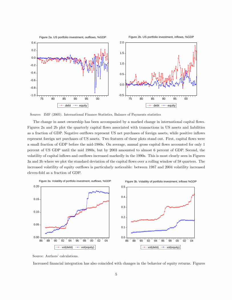
The change in asset ownership has been accompanied by a marked change in international capital flows.

Figures 2a and 2b plot the quarterly capital flows associated with transactions in US assets and liabilities

as a fraction of GDP. Negative outflows represent US net purchases of foreign assets, while positive inflows

represent foreign net purchases of US assets. Two features of these plots stand out. First, capital flows were

a small fraction of GDP before the mid-1980s. On average, annual gross capital flows accounted for only 1

percent of US GDP until the mid 1980s, but by 2003 amounted to almost 6 percent of GDP. Second, the

volatility of capital inflows and outflows increased markedly in the 1990s. This is most clearly seen in Figures

3a and 3b where we plot the standard deviation of the capital flows over a rolling window of 58 quarters. The

increased volatility of equity outflows is particularly noticeable: between 1987 and 2004 volatility increased

eleven-fold as a fraction of GDP.

0.00

0.05

0.10

0.15

0.20

86 88 90 92 94 96 98 00 02 04

vol(debt) vol(equity)

Figure 3a. Volatility of portfolio investment, outflows, %GDP

0.0

0.1

0.2

0.3

0.4

0.5

86 88 90 92 94 96 98 00 02 04

vol(debt) vol(equity)

Figure 3b. Volatility of portfolio investment, inflows %GDP

Source: Authors’ calculations.

Increased financial integration has also coincided with changes in the behavior of equity returns. Figures

5

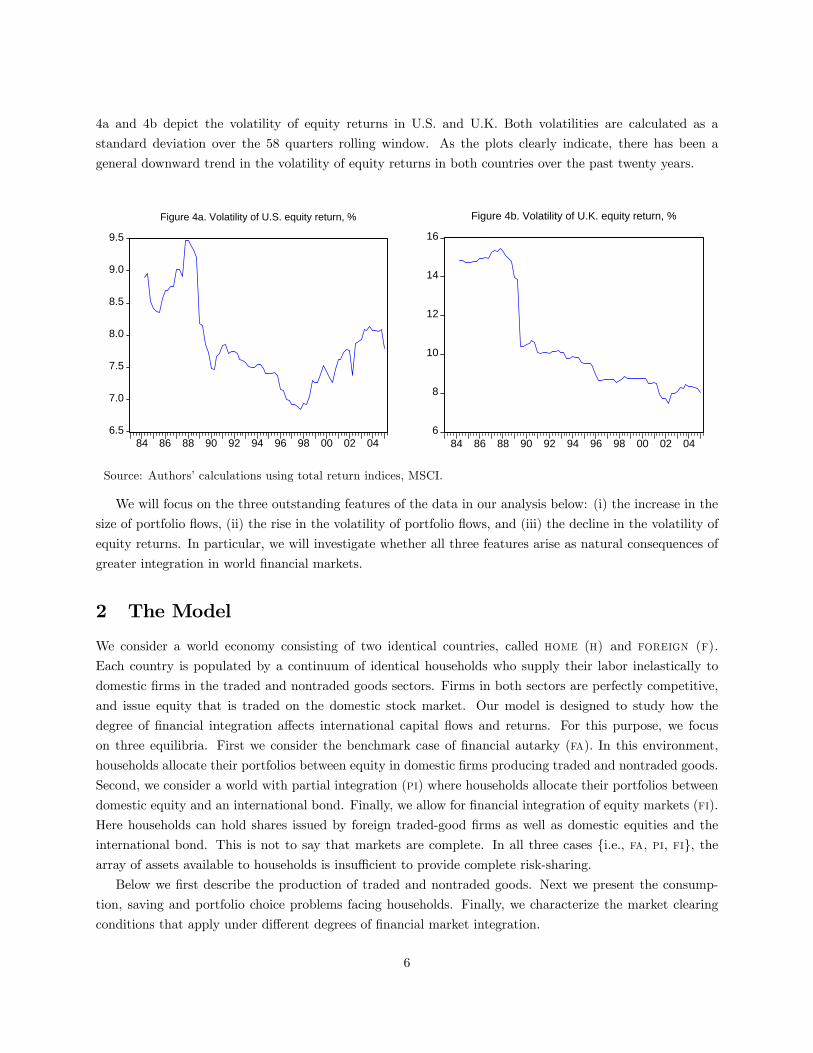
4a and 4b depict the volatility of equity returns in U.S. and U.K. Both volatilities are calculated as a

standard deviation over the 58 quarters rolling window. As the plots clearly indicate, there has been a

general downward trend in the volatility of equity returns in both countries over the past twenty years.

6.5

7.0

7.5

8.0

8.5

9.0

9.5

84 86 88 90 92 94 96 98 00 02 04

Figure 4a. Volatility of U.S. equity return, %

6

8

10

12

14

16

84 86 88 90 92 94 96 98 00 02 04

Figure 4b. Volatility of U.K. equity return, %

Source: Authors’ calculations using total return indices, MSCI.

We will focus on the three outstanding features of the data in our analysis below: (i) the increase in the

size of portfolio flows, (ii) the rise in the volatility of portfolio flows, and (iii) the decline in the volatility of

equity returns. In particular, we will investigate whether all three features arise as natural consequences of

greater integration in world financial markets.

2 The Model

We consider a world economy consisting of two identical countries, called home (h) and foreign (f).

Each country is populated by a continuum of identical households who supply their labor inelastically to

domestic firms in the traded and nontraded goods sectors. Firms in both sectors are perfectly competitive,

and issue equity that is traded on the domestic stock market. Our model is designed to study how the

degree of financial integration affects international capital flows and returns. For this purpose, we focus

on three equilibria. First we consider the benchmark case of financial autarky (fa). In this environment,

households allocate their portfolios between equity in domestic firms producing traded and nontraded goods.

Second, we consider a world with partial integration (pi) where households allocate their portfolios between

domestic equity and an international bond. Finally, we allow for financial integration of equity markets (fi).

Here households can hold shares issued by foreign traded-good firms as well as domestic equities and the

international bond. This is not to say that markets are complete. In all three cases i.e., fa, pi, fi, the

array of assets available to households is insufficient to provide complete risk-sharing.

Below we first describe the production of traded and nontraded goods. Next we present the consump-

tion, saving and portfolio choice problems facing households. Finally, we characterize the market clearing

conditions that apply under different degrees of financial market integration.

6

2.1 Production

The traded goods sector in each country is populated by a continuum of identical firms. Each firm owns its

own capital and issues equity on the domestic stock market. Period t production by a representative firm in

the traded goods sector of the h country is

Y tt = ZttK

θt , (1)

with θ > 0, where Kt denotes the stock of physical capital at the start of the period, and Ztt is the

exogenous state of productivity. The output of traded goods in the f country, Y tt , is given by an identical

production function using foreign capital Kt, and productivity Ztt . Hereafter we use “ˆ” to denote foreign

variables. The traded goods produced by h and f firms are identical and can be costlessly transported

between countries. Under these conditions, the law of one price must prevail for traded goods to eliminate

arbitrage opportunities.

At the beginning of each period, traded goods firms observe the current state of productivity, and then

decide how to allocate output between consumption and investment goods. Output allocated to consumption

is supplied competitively to domestic and foreign households and the proceeds are used to finance dividend

payments to the owner’s of the firm’s equity. Output allocated to investment adds to the stock of physical

capital available for production next period. We assume that firms allocate output to maximize the value of

the firm to its shareholders.

Let P tt denote the ex-dividend price of a share in the representative h firm producing traded-goods at

the start of period t, and let Dtt be the dividend per share paid at period t. P tt and Dt

t are measured in

terms of h traded goods. We normalize the number of shares issued by the representative traded-good firm

to unity so the value of the firm at the start of period t is P tt +Dtt . h firms allocate output to investment,

It, by solving

maxIt(Dt

t + P tt ) , (2)

subject to Kt+1 = (1− δ)Kt + It,

Dtt = ZttK

θt − It,

where δ > 0 is the depreciation rate on physical capital. The representative firm in the f traded goods sector

choose investment It to solve an analogous problem. Notice that firms do not have the option of financing

additional investment through the issuance of additional equity or corporate debt. Additional investment

can only be undertaken at the expense of current dividends.

The production of nontraded goods does not require any capital. The output of nontraded goods by

representative firms in countries h and f is given by

Y nt = κZnt , (3a)

Y nt = κZnt , (3b)

where κ > 0 is a constant. Znt and Znt denote the period t state of nontraded good productivity in countries

h and f respectively. The output of nontraded goods can only be consumed by domestic households. The

7

resulting proceeds are then distributed in the form of dividends to owners of equity. As above, we normalize

the number of shares issued by the representative firms to unity, so period t dividends for h firms are

Dnt = Y n

t , and for f firms are Dnt = Y n

t . We denote the ex-dividend price of a share in the representative h

and f firm, measured in terms of nontraded goods, as P nt and P nt respectively.

Productivity in the traded and nontraded good sectors is governed by an exogenous productivity process.

In particular, we assume that the vector zt ≡ [lnZtt , ln Ztt , lnZnt , ln Znt ]0 follows an AR(1) process:

zt = azt−1 + et, (4)

where et is a (4× 1) vector of i.i.d. normally distributed, mean zero shocks with covariance Ωe.

2.2 Households

Each country is populated by a continuum of households who have identical preferences over the consumption

of traded and nontraded goods. The preferences of a representative household in country h are given by

Ut = Et∞Xi=0

βiU(Ctt+i, Cnt+i), (5)

where 0 < β < 1 is the discount factor, and U(.) is a concave sub-utility function defined over the consumption

of traded and nontraded goods, Ctt and Cnt :

U(Ct, Cn) =1

φlnhλ1−φt (Ct)

φ+ λ1−φn (Cn)

φi,

with φ < 1. λt and λn are the weights the household assigns to tradable and nontradable consumption

respectively. The elasticity of substitution between tradable and nontradable consumption is (1− φ)−1 > 0.

Preferences for households in country f are similarly defined in terms of foreign consumption of tradables

and nontradables, Ctt and Cnt .

The array of financial assets available to households differs according to the degree of financial integration.

Under financial autarky (fa), households can hold their wealth in the form of equity issued by domestic

firms in the traded and nontraded goods sectors. Under partial integration (pi), households can hold

internationally traded bonds in addition to their domestic equity holdings. The third case we consider is

that of full integration (fi). Here households can hold domestic equity, international bonds and equity issued

by firms in the foreign traded-goods sector.

The household budget constraint associated with each of these different financial structures can be written

in a simple common form. In the case of the representative h household, we write

Wt+1 = Rwt+1 (Wt − Ctt −QntCnt ) , (6)

where Qnt is the relative price of h nontradables in terms of tradables. Rwt+1 is the (gross) return on wealth

between period t and t + 1, where wealth, Wt, is measured in terms of tradables. The return on wealth

depends on how the household allocates wealth across the available array of financial assets, and on the

8

realized return on those assets. In the fi case, the return is given by

Rwt+1 = Rt + αtt (Rtt+1 −Rt) + αtt (R

tt+1 −Rt) + αnt (R

nt+1 −Rt), (7)

where Rt is the return on bonds, Rtt+1 and Rtt+1 are the returns on h and f tradable equity, and R

nt+1 is the

return on h nontradable equity. The fraction of wealth held in h and f tradable equity and h nontradable

equity are αtt , αtt and αnt respectively. In the pi case, h households cannot hold f tradable equity, so α

tt = 0.

Under fa, households can only hold domestic equity, so αtt = 0 and αtt + αnt = 1.

The budget constraint for f households is similarly represented by

Wt+1 = Rwt+1(Wt − Ctt − Qnt Cnt ), (8)

with Rwt+1 = Rt + αtt (Rtt+1 −Rt) + αtt (R

tt+1 −Rt) + αnt (R

nt+1 −Rt), (9)

where Rtt+1, and Rtt+1 denote the return on h and f tradable equity, and R

nt+1 is the return on f nontradable

equity. Although these returns are also measured in terms of tradables, they can differ from the returns

available to h households. In particular, the returns on nontradable equity received by f households, Rnt+1,

will in general differ from the returns received by h households because the assets are not internationally

traded. Arbitrage will equalize returns in other cases. In particular, if bonds are traded, the interest received

by h and f households must be the same as (7) and (9) show. Similarly, arbitrage will equalize the returns

on tradable equity in the case of pi and fi so that Rtt+1 = Rtt+1 and Rtt+1 = Rtt+1.

2.3 Market Clearing

The market clearing requirements of the model are most easily stated if we normalize the national populations

to unity, as well as the population of firms in the tradable and nontradable sectors. Output and consumption

of traded and nontraded goods can now be represented by the output and consumption of representative

households and firms. In particular, the market clearing conditions in the nontradable sector of each country

are given by

Cnt = Y nt , and Cnt = Y n

t . (10)

Recall that firms in the nontraded sector pay dividends to their shareholders with the proceeds from the sale

of nontradables to households. Thus, market clearing in the nontraded sector also implies that

Dnt = Y n

t , and Dnt = Y n

t . (11)

The market clearing conditions in the tradable goods market are equally straightforward. Recall that the

traded goods produced by h and f firms are identical and can be costlessly transported between countries.

Market clearing therefore requires that the world demand for tradables equals world output less the amount

allocated to investment:

Ctt + Ctt = Y tt + Y t

t − It − It. (12)

Next, we turn to market clearing in financial markets. Let Att , Att and A

nt denote the number of shares of

h tradable, f tradable and h nontradable firms held by h households between the end of periods t and t+1.

9

f household share holdings in h tradable, f tradable and f nontradable firms are represented by Att , Att and

Ant . h and f household holdings of bonds between the end of periods t and t+ 1 are denoted by Bt and Bt.

Household demand for equity and bonds are determined by their optimal choice of portfolio shares (i.e., αtt ,

αtt and αnt for h households, and αtt , αtt and αnt for f households) described below. We assume that bonds

are in zero net supply. We also normalized the number of outstanding shares issued by firms in each sector

to unity.

The market clearing conditions in financial markets vary according to the degree of financial integration.

Under fa, households can only hold the equity issued by domestically located firms, so the equity market

clearing conditions are

home: 1 = Att , 0 = Att , and 1 = Ant , (13a)

foreign: 0 = Att , 1 = Att , and 1 = Ant , (13b)

while bond market clearing requires that

0 = Bt, and 0 = Bt. (14)

Notice that fa rules out the possibility of international borrowing or lending, so neither country can run at

positive or negative trade balance. Domestic consumption of tradables must therefore equal the fraction of

tradable output not allocated to investment. Hence, market clearing under fa also implies that

Dtt = Ctt , and Dt

t = Ctt . (15)

Under pi, households can hold bonds in addition to domestic equity holdings. In this case, equity market

clearing requires the conditions in (13), but the bond market clearing condition becomes

0 = Bt + Bt. (16)

The bond market can now act as the medium for international borrowing and lending, so there is no longer

a balanced trade requirement restricting dividends. Instead, the goods market clearing condition in (12)

implies that

Dtt + Dt

t = Ctt + Ctt . (17)

Under fi, households have access to domestic equity, international bonds and equity issued by firms in

the foreign tradable sector. In this case market clearing in equity markets requires that

tradable : 1 = Att + Att , and 1 = Att + Att , (18a)

nontradable : 1 = Ant , and 1 = Ant . (18b)

Market clearing in the bond market continues to require condition (16) so tradable dividends satisfy (17).

In this case international borrowing and lending takes place via trade in international bonds and the equity

of h and f firms producing tradable goods.

10

3 Equilibrium

An equilibrium in our world comprises a set of asset prices and relative goods prices that clear markets

given the state of productivity, the optimal investment decisions of firms producing tradable goods, and the

optimal consumption, savings and portfolios decisions of households. Since markets are incomplete under all

three levels of financial integration we consider, an equilibrium can only be found by solving the firm and

households’ problems for a conjectured set of equilibrium price processes, and then checking that resulting

decisions are indeed consistent with market clearing. In this section, we first characterize the solutions to the

optimization problems facing households and firms. We then describe a procedure for finding the equilibrium

price processes.

3.1 Consumption, Portfolio and Dividend Choices

Consider the problem facing a h household under fa. In this case the h household chooses consumption

of tradable and nontradable goods, Ctt and Cnt , and portfolio shares for equity in h and f firms producing

tradables and h firms producing nontradables, αtt , αtt and αnt , to maximize expected utility (5) subject to

(6) and (7) given current equity prices, P tt P tt , Pnt , the interest rate on bonds, Rt, and the relative price

of nontradables Qnt . The first order conditions for this problem are

Qnt =∂U/∂Cnt∂U/∂Ctt

, (19a)

1 = Et£Mt+1R

tt+1

¤, (19b)

1 = Et£Mt+1R

nt+1

¤, (19c)

1 = Et [Mt+1Rt] , (19d)

1 = EthMt+1R

tt+1

i, (19e)

where Mt+1 ≡ β¡∂U/∂Ctt+1

¢/ (∂U/∂Ctt ) is the discounted intertemporal marginal rate of substitution

(IMRS) between the consumption of tradables in period t and period t + 1. Condition (19a) equates the

relative price of nontradables to the marginal rate of substitution between the consumption of tradables

and nontradables. Under fa, consumption and portfolio decisions are completely characterized by (19a) -

(19c). When households are given access to international bonds under pi, there is an extra dimension to

the portfolio choice problem facing households so (19d) is added to the set of first order conditions. Under

fi, all the conditions in (19) are needed to characterize optimal h household behavior. An analogous set of

conditions characterize the behavior of f households.

It is important to note that all the returns in (19) are measured in terms of tradables. In particular, the

return on the equity of firms producing tradable goods in the h and f counties held by h investors are

Rtt+1 =¡P tt+1 +Dt

t+1

¢/P tt , and Rtt+1 =

³P tt+1 + Dt

t+1

´/P tt . (20)

Because the law of one price applies to tradable goods, these equations also define the return f households

receive on their equity holdings in h and f firms producing tradable goods. In other words, Rtt+1 = Rtt+1and Rtt+1 = Rtt+1. The law of one price similarly implies that the return on bonds Rt is the same for all

11

households.

The returns on equity producing nontradable goods differ across countries. In particular, the return on

equity for h households is

Rnt+1 =©¡P nt+1 +Dn

t+1

¢/P nt

ª©Qnt+1/Q

nt

ª, (21)

while for f households the return is

Rnt+1 =n³

P nt+1 + Dnt+1

´/P nt

onQnt+1/Q

nt

o, (22)

where Qnt is the relative price of nontradables in country f.

The returns Rnt+1 and Rnt+1 differ from each other for two reasons: First, international productivity

differentials in the nontradable sectors will create differences in returns measured in terms of nontradables.

These differences will affect returns via the first term on the right hand side of (21) and (22). Second,

international differences in the dynamics of relative prices Qnt and Qnt will affect returns via the second term

in each equation. These differences arise quite naturally in equilibrium as the result of productivity shocks

in either the tradable or nontradable sectors.

Variations in the relative prices of nontraded goods also drive the real exchange rate, which is defined as

the ratio of price indices in the two countries:

Qt =

(λT + λN (Q

nt )

φφ−1

λT + λN (Qnt )φ

φ−1

)φ−1φ

. (23)

The returns on equity shown in (20) - (22) are functions of equity prices, the relative price of nontradables,

and the dividends paid by firms. The requirements of market clearing and our specification for the production

of nontraded goods implies that dividends Dnt+1 and D

nt+1 are exogenous. By contrast, the dividends paid by

firms producing tradable goods are determined optimally. Recall that h firms choose real investment It in

period t to maximize the current value of the firm, Dtt +P tt . Combining (19b) with the definition of returns

Rtt+1 in (20) implies that Ptt = Et

£Mt+1

¡P tt+1 +Dt

t+1

¢¤. This equation identifies the price a h household

would pay for equity in the firm (after period t dividends have been paid). Using this expression to substitute

for P tt in the h firm’s investment problem (2) gives the following first order condition:

1 = EthMt+1

³θZtt+1 (Kt+1)

θ−1+ (1− δ)

´i. (24)

This condition implicitly identifies the optimal level of dividends in period t because next period’s capital

depends on current capital, productivity and dividend payments: Kt+1 = (1−δ)Kt+ZttKθt −Dt

t . Dividends

on the equity of f firms producing tradable goods is similarly determined by

1 = EthMt+1

³θZtt+1(Kt+1)

θ−1 + (1− δ)´i

, (25)

where Mt+1 is the IMRS for tradable goods in country f, and Kt+1 = (1− δ)Kt + Ztt Kθt − Dt

t .

The dividend policies implied by (24) and (25) maximize the value of each firm from the perspective of

domestic shareholders. For example, the stream of dividends implied by (24) maximizes the value of h firms

12

producing traded goods for households in country h because the firm uses Mt+1 to value future dividends.

This is an innocuous assumption under financial autarky and partial integration because domestic households

must hold all the firm’s equity. Under full integration, however, foreign households have the opportunity to

hold the h firm’s equity so the firm’s dividend policy need not maximize the value of equity to all shareholders.

In particular, since markets are incomplete even under full integration, the IMRS for h and f households

will differ, so f households holding domestic equity will generally prefer a different dividend stream from the

one implied by (24). In short, the dividend streams implied by (24) and (25) incorporate a form of home

bias because they focus exclusively on the interests of domestic shareholders.

We can now summarize the equilibrium actions of firms and households. At the beginning of period

t, firms in the traded-goods sector observe the new level of productivity and decide on the amount of

real investment to undertake. This decision determines dividend payments Dtt and Dt

t as a function of

existing productivity, physical capital, expectations regarding future productivity and the IMRS of domestic

shareholders. Firms in the nontradable sectors have no real investment decision to make so in equilibriumDnt

and Dnt depend only on current productivity. At the same time, households begin period t with a portfolio

of financial assets. Under fa the menu of assets is restricted to domestic equities, under pi households may

hold domestic equities and bonds, and under fi the menu may contain domestic equity, foreign equity and

bonds. Households receive dividend payments from firms according to the composition of their portfolios.

They then make consumption and new portfolio decisions based on the market clearing relative price for

nontradables, and the market-clearing prices for equity. The first-order conditions in (19) implicitly identify

the decisions made by h households. The decisions made by f households are characterized by an analogous

set of equations. The portfolio shares determined in this manner will depend on household expectations

concerning future returns and the IMRS. As equations (20) - (22) show, equity returns are a function of

current equity prices and future dividends and prices, so expectations regarding the latter will be important

for determining how households choose portfolios in period t. Current and future consumption decisions also

affect period t portfolio shares through the IMRS. Households’ demand for financial assets in period t follows

from decisions on consumption and the portfolio shares in a straightforward manner. In the case of fi, the

demand for each asset from h and f households is

h households f households

h tradable equity: Att = αttWct /P

tt , Att = αtt W

ct /P

tt ,

f tradable equity: Att = αttWct /P

tt , Att = αtt W

ct /P

tt ,

nontradable equity: Ant = αntWct /Q

ntP

nt , Ant = αnt W

ct /Q

nt P

nt ,

bonds Bt = αbtWct Rt, Bt = αbt W

ct Rt,

(26)

where W ct ≡ Wt − Ctt − QntC

nt and W c

t ≡ Wt − Ctt − Qnt Cnt denote period t wealth net of consumption

expenditure with αbt ≡ 1 − αtt − αtt − αnt and αbt ≡ 1 − αtt − αtt − αnt . Equation (26) shows that asset

demands depend on expected future returns and risk via optimally chosen portfolio shares, αt, accumulated

net wealth W ct and W c

t , and current asset prices (i.e., Ptt , P

tt , P

nt and P nt for equity, and 1/Rt for bonds).

13

3.2 Equilibrium Dynamics

Finding an equilibrium in this model is conceptually straightforward. All that is required are the time

series processes for equity prices P tt , Ptt , P

nt and P

nt , the relative prices of nontradables Qnt and Qnt , and

interest rate on bonds Rt, that clear markets given the optimal behavior of firms and households. Finding

these time series in practice is complicated by the need to completely characterize how firms and households

behave. When markets are complete, this complication can be circumvented by finding the equilibrium

allocations as the solution of an appropriate social planning problem and then deriving the price and interest

rates processes that support these allocations when decision—making is decentralized. This solution method

is inapplicable in our model. When markets are incomplete, as they under fa, pi, and fi, there is no way to

formulate a social planning problem that will provide the equilibrium allocation of the decentralized market

economy. To solve the model, we must therefore characterize the optimal behavior of firms and households

for a wide class of price and interest rate processes, and then use the implied allocations in conjunction

with the market clearing conditions to find the particular set of price and interest rate processes that clear

markets. We implement this solution procedure as follows.

Our first step is to conjecture the form of the vector of state variables that characterize the equilibrium

dynamics of the economy. For this purpose, let kt ≡ ln (Kt/K) and kt = ln³Kt/K

´where K is the steady

state capital stock for firms producing tradable goods. We posit that the state vector is given by

xt = [zt, kt, kt, wt, wt]0,

where wt ≡ ln(Wt/W0), wt ≡ ln(Wt/W0) and zt ≡ [lnZtt , ln Ztt , lnZnt , ln Znt ]0. Our conjecture for xt containsthe current state of productivity, the capital stocks in the h and f traded-goods sectors relative to their

steady state levels, and the wealth of h and f households relative to their initial levels W0 and W0. All eight

variables are needed to characterize period t decisions and market—clearing prices.

The next step is to characterize the dynamics of xt. Nonlinearities in our model make it impossible

to describe the dynamics of xt using just its own lagged values. When households face portfolio choice

problems, wealth in period t will depend on the first and second moments of returns conditioned on period

t − 1 information. In general, these moments will be high order polynomials in the elements of xt−1 (e.g.,w2t−1, w

2t−1, wt−1wt−1, ..., w

3t−1, ...), so elements of xt will depend on not just xt−1 but also elements in

xt−1x0t−1 and so on. We consider an approximate solution to the model that ignores the impact of third

and higher order terms. Under this assumption, we conjecture that the dynamics of the economy can be

summarized by

Xt+1 = AXt + Ut+1, (27)

whereXt+1 ≡ [ 1 x0t+1 x0t+1 ]0, xt+1 ≡ vec

¡xt+1x

0t+1

¢and Ut+1 is a vector of shocks with E [Ut+1|Xt] = 0,

and E£Ut+1U

0t+1|Xt

¤= S(Xt). Equation (27) describes the approximate dynamics of the augmented state

vector Xt that contains a constant, the original state vector xt and all the cross-products of xt in xt. Notice

that Xt+1 depends linearly on lagged Xt so forecasting future states of the economy is straightforward:

E [Xt+1|Xt] = AXt. Since firms and households based their period t decisions on expectations concerning

variables in t+1, this aspect of (27) is useful when checking the optimality of decision-making. Equation (27)

also introduces conditional heteroskedasticity into the state variables via the S(.) function. Heteroskedasticity

14

arises endogenously in our model if households change the composition of their portfolios, so our conjecture

for the equilibrium dynamics of the state variables must allow the covariance of Ut+1 to vary with elements

of Xt.

The final step is to find the elements of the A matrix and the covariance function S(.) implied by theequilibrium of the model. Some elements of A and S(.) are simple functions of the model’s parameters,others depend on the decisions made by households and firms. To find these elements, we use the method of

undetermined coefficients. Specifically, we posit that the log dividend, log consumption and portfolio shares

in period t can be written as particular linear functions of the augmented state vector, Xt. With these

functions we can then characterize the dynamics of capital and wealth from period to period, and hence fill

in all the unknown elements of the A matrix and the covariance function S(.).We also use the assumed formof period t decisions in conjunction with the market clearing conditions to derive expressions for equilibrium

equity prices, relative prices and the interest rate as log linear functions of Xt. Lastly, we verify that the

assumed form of the period t decisions are consistent with the firm and household first order conditions

given the equilibrium price and return dynamics implied by (27). Evans and Hnatkovska (2005) provides a

detailed description of this procedure.

Two further aspects of this solution procedure deserve emphasis. First, it does not make any assumption

about the stationarity of individual state variables. In the calibrated version of the model we examine below,

productivity is assumed to follow a stationary process, but capital and wealth are free for follow unit root

processes in equilibrium. This turns out to be a useful feature of the procedure. As we discuss in detail

below, there are good economic reasons for transitory shocks to productivity to have permanent effects

on equilibrium wealth in our model. So a solution procedure that imposed stationarity on wealth would

be inappropriate. Our procedure allows for these permanent wealth effects but in a limited manner. The

limitation arises from the second important aspect of our procedure, namely its use of (27). This equation

approximates the equilibrium dynamics of the economy under the assumption that terms involving third and

higher order powers of the state variables have negligible impact on the elements of xt. This is reasonable

along a sample path where all the elements of xt are small. However, our specification for xt contains the log

deviation of household wealth from its initial level, wt and wt, so a sequence of transitory productivity shocks

could push wt and wt permanently far from zero. At this point the dynamics of Xt are poorly approximated

by (27) and our characterization of the equilibrium would be unreliable. In this sense (27) approximates the

dynamics of the economy in a neighborhood of the initial distribution of wealth. We are cognizant of this

fact when studying the equilibrium dynamics below. In particular, when simulating the model we check that

the sample paths for wealth and capital remain in a neighborhood of their initial distributions so that third

order terms are unimportant.

Our solutions to the model use the parameter values summarized in Table 1. We assume that household

preferences and firm technologies are symmetric across the two countries, and calibrate the model for a

period equalling one quarter. The value for φ is chosen to set the intratemporal elasticity of substitution

between tradables and nontradables at 0.74, consistent with the value in Corsetti, Dedola and Leduc (2003).

The share parameters for traded and nontraded goods, λt and λn, are both set to 0.5, and the discount factor

β equals 0.99. On the production side, we set the capital share in tradable production θ to 0.36, and the

depreciation rate δ to 0.02. These values are consistent with the estimates in Backus, Kehoe and Kydland

(1995). The only other parameters in the model govern the productivity process. We assume that each of

15

the four productivity processes (i.e. lnZtt , ln Ztt , lnZ

nt , and ln Z

nt ) follow AR(1) processes with independent

shocks. The AR(1) coefficients in the processes for tradable—goods productivity, lnZtt and ln Ztt , are 0.78,

while the coefficients for nontradable productivity, lnZnt , and ln Znt , are 0.99. Shocks to all four productivity

process have a variance of 0.0001. This specification implies that all shocks have persistent but temporary

affects on productivity. Any permanent effects they have on other variables must arise endogenously from

the structure of the model.

Table 1: Model Parameters

Preferences β λt λn 1/(1− φ)0.99 0.5 0.5 0.74

Production θ δ0.36 0.02

Productivity atii anii Ωe0.78 0.99 0.0001

4 Results

We analyze the equilibrium properties of our model in three steps. First, we examine how the economy

responds to productivity shocks. Next, we study the behavior of international capital flows. Finally, we

examine the implications of differing degrees of integration for the behavior of asset prices and returns.

4.1 Risk-Sharing and Financial Integration

The consequences of greater financial integration are most easily understood by considering how the economy

responds to productivity shocks. With this in mind, consider how a positive productivity shock to domestic

firms producing traded goods affects real output and consumption in both countries under our three market

configurations. The effects on the current account and the relative price of tradables are shown in the left

hand panels of Figure 5a4. Recall that productivity shocks only have temporary affects on the marginal

product of capital. Thus, a positive productivity shock in the domestic traded-goods sector will induce an

immediate one-period rise in real investment as firms in that sector take advantage of the temporarily high

marginal product of capital. In short, there is an investment boom in the domestic tradable goods sector.

Because the equity issued by these firms represents a claim on the future dividend stream sustained by the

firm’s capital stock, one effect of the investment boom is to increase the equilibrium price of tradable equity

4The current account in country h is calculated from the individual’s budget constraint as the sum of net exports and netforeign income: CAt = Dt

t − Ctt + (DttA

tt−1 − Dt

t Att−1). The current account is also identically equal to the change in net

foreign asset position: CAt = P tt ∆Att −P tt ∆Att + (1Rt

Bt −Bt−1). Under pi, the current account is equal to the trade balance,

which in turn equals the change in bond holdings: CAt = Dtt −Ctt =

1Rt

Bt −Bt−1.

16

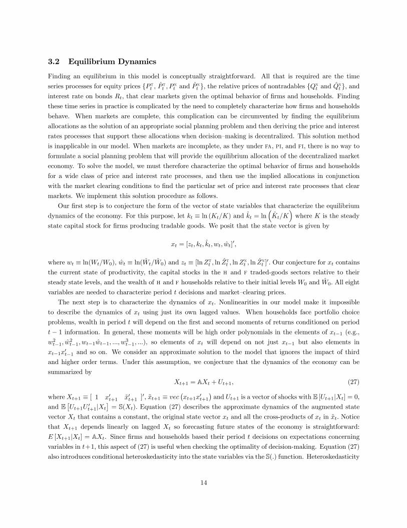
P tt . Under fa, this capital gain raises the wealth of h households so the domestic demand for both tradable

and nontradable goods increase. While increased domestic output can accommodate the rise in demand for

tradables, there is no change in the output of nontradables, so the relative price of nontradables, Qnt , must

rise to clear domestic goods markets.

Figure 5a. Real effects of productivity shocks

A similar adjustment pattern occurs under pi. The capital gain enjoyed by h households again translates

into increased demand for tradables and nontradables, but now the demand for tradables can be accom-

modated by both h and f firms producing tradables. As a result, the productivity shock is accompanied

by a trade deficit in the h country and a smaller rise in Qnt than under fa. Once the investment boom is

over, the domestic supply of tradables available for consumption rises sharply above domestic consumption.

From this point on, the h country runs a trade surplus. Initially, this surplus is used to pay off the foreign

debt incurred during the investment boom. Once this is done, h households start lending to f households

by buying bonds. This allows h households to smooth the consumption gains from the productive shock far

beyond the point where its direct effects on domestic output disappear. As a consequence, the temporary

shock to productivity has permanent effects on the international distribution of wealth.

In the case of fi, the increase in P tt represents a capital gain to both h and f households because

everyone diversifies their international equity holdings (i.e., all households hold equity issued by h and f firms

producing tradable goods). As a result, the demand for tradables and nontradables rise in both countries. At

the same time, by taking a fully diversified positions in t equities, households in both countries can finance

17

higher tradable consumption without borrowing from abroad. As the trade deficit is exactly offset by the

positive net foreign income, the current account remains in balance.5 Market clearing in the nontradable

markets raises relative prices (i.e. Qnt and Qnt ), but less than under pi.

The right hand panels of Figure 5a show the effects of positive productivity shock in the h nontradable

sector. Once again, the shock produces a trade and current account deficits under pi, but it is much smaller

and persists for much longer than the deficit associated with productivity shocks in the tradable sector. The

reason for this difference arises from the absence of an investment boom. A positive productivity shock in

h nontradables increases the supply of nontradable output available for domestic consumption. This has

two equilibrium effects. First, it lowers the relative price of nontradables, Qnt , so that the h market for

nontradables clears. This is clearly seen in the lower right hand panel of Figure 5a. Second, it raises the

h demand for tradables because tradables and nontradables are complementary. The result is a persistent

trade and current account deficit. Under fi, a productivity increase in n sector leads to a current account

deficit. On impact, the size of the deficit is comparable with that under pi, and likewise is financed by

borrowing from abroad. However, the amount of such borrowing under fi is much larger as it is used to

finance both consumption demand and purchases of a diversified portfolio of t equity shares. Immediately

after the shock, the current account deficit falls by more than 50% as dividends on foreign equities flow in.

Thereafter, it slowly reverts back to zero.

To summarize, the current account dynamics displayed in Figure 5a are readily understood in terms

of intertemporal consumption smoothing once we recognize that shocks to tradable productivity induce

domestic investment booms. In addition, these dynamics differ under the pi and fi configurations. When

given a choice between international bonds and equity, households choose to take fully diversified positions

in stocks allowing them to share country specific risks internationally. Then, depending on the productivity

shock, bonds are either used to finance the purchases of equity, or become redundant. When equity is not

available, bonds must be used to smooth consumption.

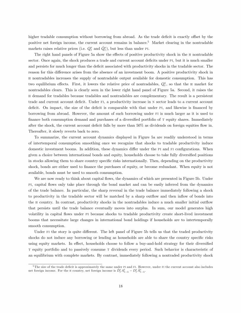
We are now ready to think about capital flows, the dynamics of which are presented in Figure 5b. Under

pi, capital flows only take place through the bond market and can be easily inferred from the dynamics

of the trade balance. In particular, the sharp reversal in the trade balance immediately following a shock

to productivity in the tradable sector will be matched by a sharp outflow and then inflow of bonds into

the h country. In contrast, productivity shocks in the nontradables induce a much smaller initial outflow

that persists until the trade balance eventually moves into surplus. In sum, our model generates high

volatility in capital flows under pi because shocks to tradable productivity create short-lived investment

booms that necessitate large changes in international bond holdings if households are to intertemporally

smooth consumption.

Under fi the story is quite different. The left panel of Figure 5b tells us that the traded productivity

shocks do not induce any borrowing or lending as households are able to share the country specific risks

using equity markets. In effect, households choose to follow a buy-and-hold strategy for their diversified

t equity portfolio and to passively consume t dividends every period. Such behavior is characteristic of

an equilibrium with complete markets. By contrast, immediately following a nontraded productivity shock

5The size of the trade deficit is approximately the same under pi and fi. However, under fi the current account also includesnet foreign income. For the h country, net foreign income is Dt

tAtt−1 −Dt

t Att−1.

18

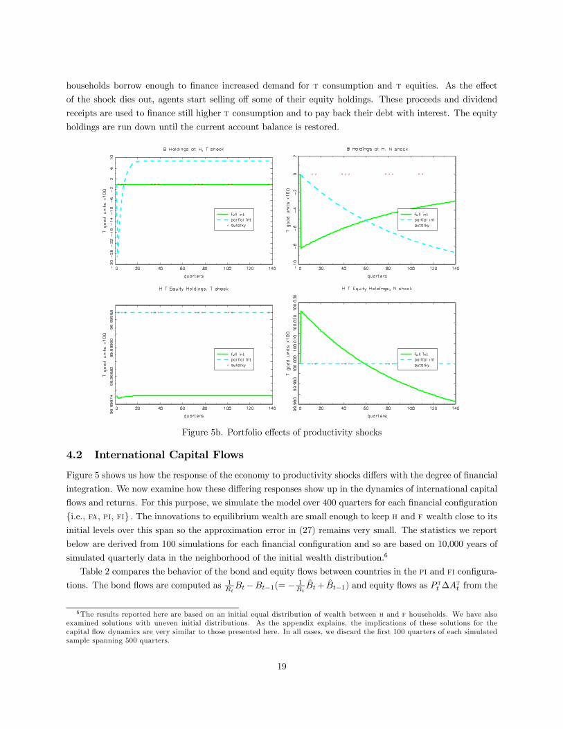
households borrow enough to finance increased demand for t consumption and t equities. As the effect

of the shock dies out, agents start selling off some of their equity holdings. These proceeds and dividend

receipts are used to finance still higher t consumption and to pay back their debt with interest. The equity

holdings are run down until the current account balance is restored.

Figure 5b. Portfolio effects of productivity shocks

4.2 International Capital Flows

Figure 5 shows us how the response of the economy to productivity shocks differs with the degree of financial

integration. We now examine how these differing responses show up in the dynamics of international capital

flows and returns. For this purpose, we simulate the model over 400 quarters for each financial configuration

i.e., fa, pi, fi . The innovations to equilibrium wealth are small enough to keep h and f wealth close to its

initial levels over this span so the approximation error in (27) remains very small. The statistics we report

below are derived from 100 simulations for each financial configuration and so are based on 10,000 years of

simulated quarterly data in the neighborhood of the initial wealth distribution.6

Table 2 compares the behavior of the bond and equity flows between countries in the pi and fi configura-

tions. The bond flows are computed as 1RtBt−Bt−1(= − 1

RtBt+ Bt−1) and equity flows as P tt ∆A

tt from the

6The results reported here are based on an initial equal distribution of wealth between h and f households. We have alsoexamined solutions with uneven initial distributions. As the appendix explains, the implications of these solutions for thecapital flow dynamics are very similar to those presented here. In all cases, we discard the first 100 quarters of each simulatedsample spanning 500 quarters.

19

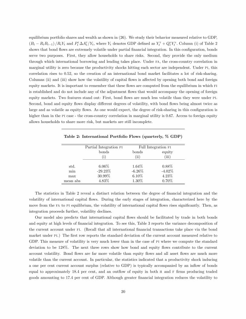
equilibrium portfolio shares and wealth as shown in (26). We study their behavior measured relative to GDP,

(Bt −RtBt−1) /RtYt and P tt ∆Att /Yt, where Yt denotes GDP defined as Y

tt +Qnt Y

nt . Column (i) of Table 2

shows that bond flows are extremely volatile under partial financial integration. In this configuration, bonds

serve two purposes. First, they allow households to share risks. Second, they provide the only medium

through which international borrowing and lending takes place. Under fa, the cross-country correlation in

marginal utility is zero because the productivity shocks hitting each sector are independent. Under pi, this

correlation rises to 0.52, so the creation of an international bond market facilitates a lot of risk-sharing.

Columns (ii) and (iii) show how the volatility of capital flows is affected by opening both bond and foreign

equity markets. It is important to remember that these flows are computed from the equilibrium in which fi

is established and do not include any of the adjustment flows that would accompany the opening of foreign

equity markets. Two features stand out: First, bond flows are much less volatile than they were under pi.

Second, bond and equity flows display different degrees of volatility, with bond flows being almost twice as

large and as volatile as equity flows. As one would expect, the degree of risk-sharing in this configuration is

higher than in the pi case - the cross-country correlation in marginal utility is 0.67. Access to foreign equity

allows households to share more risk, but markets are still incomplete.

Table 2: International Portfolio Flows (quarterly, % GDP)

Partial Integration pi Full Integration fibonds bonds equity(i) (ii) (iii)

std. 6.06% 1.64% 0.88%min -29.23% -6.26% -4.02%max 30.99% 6.10% 4.23%

mean abs 4.83% 1.30% 0.70%

The statistics in Table 2 reveal a distinct relation between the degree of financial integration and the

volatility of international capital flows. During the early stages of integration, characterized here by the

move from the fa to pi equilibrium, the volatility of international capital flows rises significantly. Then, as

integration proceeds further, volatility declines.

Our model also predicts that international capital flows should be facilitated by trade in both bonds

and equity at high levels of financial integration. To see this, Table 3 reports the variance decomposition of

the current account under fi. (Recall that all international financial transactions take place via the bond

market under pi.) The first row reports the standard deviation of the current account measured relative to

GDP. This measure of volatility is very much lower than in the case of pi where we compute the standard

deviation to be 128%. The next three rows show how bond and equity flows contribute to the current

account volatility. Bond flows are far more volatile than equity flows and all asset flows are much more

volatile than the current account. In particular, the statistics indicated that a productivity shock inducing

a one per cent current account surplus (relative to GDP) is typically accompanied by an inflow of bonds

equal to approximately 18.4 per cent, and an outflow of equity in both h and f firms producing traded

goods amounting to 17.4 per cent of GDP. Although greater financial integration reduces the volatility to

20

the current account by facilitating greater risk-sharing, the financial flows accompanying current account

imbalances remain sizable.

Table 3: Variance Decomposition of Current Account

Std. of Current Account 0.293%

∆ net debt, 1R1tBt −Bt−1 18.3711

∆ t equity assets, PTt ∆A

tt -8.6783

∆ t equity liabilities, −PTt ∆A

tt -8.6875

We can gain further insight into the origins of the international equity and bond flows by decomposing

each flow into two components. For this purpose, we use (26) to re-write the flow of equity in traded—good

firms as:

P tt ∆Att = αTt W

ct − αTt−1W

ct−1

PTtPTt−1

,

= ∆αTt Wct +

∙αTt−1∆W

ct −

µPTtPTt−1

− 1¶W c

t−1αTt−1

¸. (28)

The first term in the second line captures portfolio flows resulting from each household’s desire to alter

portfolio shares due to changes in expected returns and risk. Bohn and Tesar (1996) name this term the

“return chasing” component. The second term reflects each household’s intention to acquire or sell off some

of the asset when wealth changes or when there are some capital gains or losses on the existing portfolio. This

term is called the “portfolio rebalancing” component. Bond flows can be decomposed in a similar manner:

1

RtBt −Bt−1 = ∆α

btW

ct +

£αbt−1∆W

ct − (Rt−1 − 1)W c

t−1αbt−1¤. (29)

Again, the first term on the right identifies the “return chasing” component, and the second the “portfolio

rebalancing” component.

Table 4 reports the contribution each component makes to the variance of the bond and equity flows.7

The upper panel shows that variations in the “return chasing” component are the main source of volatility

in bond flows under pi. Portfolio rebalancing plays an insignificant role. This is not a surprising result.

The statistics in Table 4 are based on the equilibrium dynamics of the economy in the neighborhood of an

initial symmetric wealth distribution, so the bond position of households at the beginning of each period is

typically a small fraction of total wealth. Under these circumstances αbt−1 ∼= 0, so the second term in (29)

makes a negligible contribution to bond flows.

7More precisely, equation (28) implies that

V (P tt ∆Att ) = CV (P tt ∆Att ,∆αttWct ) +CV (P tt ∆Att , α

tt−1∆W c

t − [(P tt /P tt−1)− 1]W ct−1α

tt−1).

Table 4 reports the first and second terms on the right as a fraction of V (P tt ∆Att ) in the rows labeled “Equity”. We performa similar computation using (29) for the bond decompositions and report the results in the rows labeled “Bonds”.

21

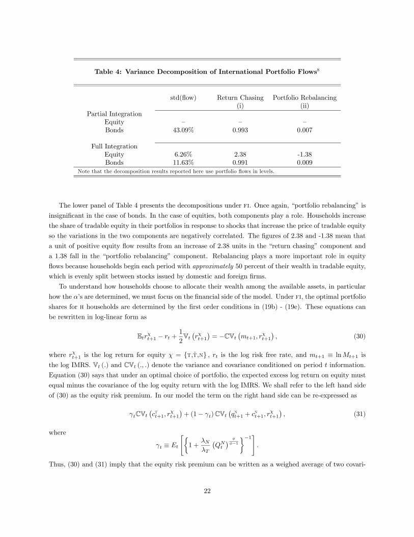
Table 4: Variance Decomposition of International Portfolio Flows8

std(flow) Return Chasing Portfolio Rebalancing(i) (ii)

Partial IntegrationEquity — — —Bonds 43.09% 0.993 0.007

Full IntegrationEquity 6.26% 2.38 -1.38Bonds 11.63% 0.991 0.009

Note that the decomposition results reported here use portfolio flows in levels.

The lower panel of Table 4 presents the decompositions under fi. Once again, “portfolio rebalancing” is

insignificant in the case of bonds. In the case of equities, both components play a role. Households increase

the share of tradable equity in their portfolios in response to shocks that increase the price of tradable equity

so the variations in the two components are negatively correlated. The figures of 2.38 and -1.38 mean that

a unit of positive equity flow results from an increase of 2.38 units in the “return chasing” component and

a 1.38 fall in the “portfolio rebalancing” component. Rebalancing plays a more important role in equity

flows because households begin each period with approximately 50 percent of their wealth in tradable equity,

which is evenly split between stocks issued by domestic and foreign firms.

To understand how households choose to allocate their wealth among the available assets, in particular

how the α’s are determined, we must focus on the financial side of the model. Under fi, the optimal portfolio

shares for h households are determined by the first order conditions in (19b) - (19e). These equations can

be rewritten in log-linear form as

Etrχt+1 − rt +1

2Vt¡rχt+1

¢= −CVt

¡mt+1, r

χt+1

¢, (30)

where rχt+1 is the log return for equity χ = t,t,n , rt is the log risk free rate, and mt+1 ≡ lnMt+1 is

the log IMRS. Vt (.) and CVt (., .) denote the variance and covariance conditioned on period t information.

Equation (30) says that under an optimal choice of portfolio, the expected excess log return on equity must

equal minus the covariance of the log equity return with the log IMRS. We shall refer to the left hand side

of (30) as the equity risk premium. In our model the term on the right hand side can be re-expressed as

γtCVt¡ctt+1, r

χt+1

¢+ (1− γt)CVt

¡qnt+1 + cnt+1, r

χt+1

¢, (31)

where

γt ≡ Et

"½1 +

λNλT

¡QNt

¢ φ

φ−1

¾−1#.

Thus, (30) and (31) imply that the equity risk premium can be written as a weighed average of two covari-

22

ances: the covariance between the log equity return and the log tradable consumption ctt+1, and covariance

between the log equity return and log nontradable consumption measured in terms of tradables, qnt+1+ cnt+1.

In principle, both covariances can change as shocks hit the economy and so can induce variations in the

equity premia. However, in practice most of the variation in the risk premia come through changes in γt.

As figure 4a showed, productivity shocks have an immediate and long-lasting effects on the relative price of

nontraded goods under fi, so they also induce variations in the equity risk premia via changes in γt.

Changes in the equity premia determine how households allocate their wealth between equities and bonds.

This is easily demonstrated once we recognize that mt+1 is perfectly correlated with log wealth, wt+1. Using

this feature of the model, we can use the household’s budget constraint to rewrite the right hand side of (30)

for χ = t,t,n . Re-arranging the resulting equations gives

αt = Σ−1t

¡Etert+1 + 1

2σ2t

¢, (32)

where αt = [αtt , α

tt , α

nt ]0 is the vector of portfolio shares, ert+1 = [rtt+1− rt, r

tt+1− rt, r

nt+1− rt]

0 is a vector of

excess equity returns, Σt is the conditional covariance of ert+1, and σ2t = diag (Σt) . Notice that Etert+1+ 12σ

2t

is just the vector of equity premia.9 Thus, the variations in Qnt induced by productivity shocks change the

equity premia and also the equilibrium portfolio shares of households. This is why the “return chasing”

component is such an important component of equity flows under fi.

4.3 Asset Prices and Returns

We now turn to examine how greater financial integration affects the behavior of asset prices and returns.

This analysis naturally complements the study of capital flows. It also provides a theoretical perspective on

the large empirical literature that uses the behavior of asset prices as a metric for measuring the degree of

financial integration between countries.

Table 5 reports the standard deviations of realized returns computed from our model simulations. Column

(i) reports volatility under fa. Here we see that the model produces far less volatility in bond and equity

returns than we observe in the world. This is not surprising given our very standard specification for

productivity, production and preferences. We do note, however, that the relative volatility of returns is

roughly in accordance with reality: equity are much more volatile than the risk free rate, and foreign

exchange returns, ∆qt ≡ lnQt − lnQt−1, are an order of magnitude more volatile than equity. Note also

that the volatility of the return on equity in firms producing nontradable goods is almost twice that of the

return on firms producing tradables.

Columns (ii) - (v) of Table 5 show how the volatility of returns change as the degree of financial integration

increases. Column (ii) reports the standard deviation of returns for the case of partial integration where

households can trade international bonds. Column (iii) shows how the volatility changes relative to the case

of fa. Opening trade in international bonds reduces the volatility of equity returns and the risk-free rate by

approximately one third, while the volatility of foreign exchange returns falls by roughly 5%. The volatility

of returns changes further when households are given access to foreign t equity. As column (v) shows, the

9Excess returns are adjusted by the addition of one half times the return variance, a Jensen’s inequality term, to accountfor the fact that we are working with log returns.

23

Table 5: Return Volatility, (annual, % std. dev.)

fa pi pi-fa difference fi fi-pi difference(i) (ii) (iii) (iv) (v)

Risk free rate rt 0.15% 0.11% -33.94% 0.11% 0.00%tradable equity rtt 0.57% 0.44% -27.17% 0.44% -0.01%nontradable equity rnt 1.09% 0.94% -14.65% 0.92% -2.77%Portfolio returns rwt 0.80% 0.64% -21.29% 0.61% -4.63%Foreign exchange ∆qt 3.75% 3.56% -5.15% 3.55% -0.17%Depositary receipt rtt 0.44% 0.44% -1.92% 0.44% -0.04%

largest changes occur in the volatility of portfolio returns (i.e., the return on wealth), which falls by 5%

relative to its level under pi. Volatility of n equity return decreases by roughly 3%.

Next, we turn to issue of how financial integration affects the relation between returns. For this purpose,

we first derive a log version of the CAPM implied by our model. Under our log specification for household

utility, the IMRS for each household is proportional to the reciprocal of the (gross) return of optimally

invested wealth, Rwt+1. Using this fact, we can rewrite the log linearized version of the h household’s first

order conditions in (19b) - (19e) as

Etrχt+1 − rt +12Vt

¡rχt+1

¢= Bχt Vt

¡rwt+1

¢(33)

where rχt+1 is the log return on equity χ = t,t,n, and rwt+1 ≡ lnRwt+1. Bχt is the beta for asset χ, defined

as the ratio of conditional covariance between asset χ and return on domestic wealth, and the conditional

variance of the market portfolio:

Bχt =CVt

¡rwt+1, r

χt+1

¢Vt¡rwt+1

¢ .

Notice that unlike the standard CAPM beta, Bχt depends on the moments of log rather than gross returns.The household first order conditions in (19b) - (19e) also imply that 1 = Et[Mt+1R

wt+1], so the approximate

relation in (33) also applies to the log return on wealth. In this case Bwt = 1, so the approximation simplifiesto

Etrwt+1 − rt =12Vt

¡rwt+1

¢. (34)

Our log version of the CAPM is obtained by combining (33) and (34):

Etrχt+1 − rt +12Vt

¡rχt+1

¢= Bχt

¡Etrwt+1 − rt +

12Vt

¡rwt+1

¢¢. (35)

This equation says that the expected log excess return on equity is proportional to the log excess return on

optimally invested wealth. Importantly, this relation is based on the optimality of households’ portfolio choice

and holds (approximately) true whatever the degree of financial integration. It therefore provides a natural

framework for examining how increased financial integration affects the relationship between equilibrium

returns.

24

We examine the effects of integration with the regression

Etrχt+1 − rt +12Vt

¡rχt+1

¢= α0 + α1Eterwt+1 + α2Eterwt+1 + α3Eterfxt+1 + ηt, (36)

for χ = t,n , where Eterit+1 ≡ Etrit+1−rt+ 12Vt

¡rit+1

¢for i = w,bw,fx. Here we consider the regression of

the expected log excess equity return on the expected log excess return on domestic wealth, Eterwt+1, foreignwealth, Eterwt+1, and the expected excess return on foreign exchange, Eterfxt+1 (where rfxt+1 ≡ qt+1 − qt). Our

CAPM equation in (35) implies that if the betas for equity are constant, the coefficients α0, α2 and α3

should equal zero, and the R2 of the regression should be very close to unity. Alternatively, if the betas are

time-varying, and those variations are unrelated to returns on foreign wealth or foreign exchange, the R2 of

the regression will be lower but α0, α2 and α3 should still equal zero. Only when the variations in the betas

are correlated with the return on foreign wealth and/or foreign exchange, will α2 and/or α3 differ from zero.

Table 6 presents the results from estimating (36) with simulated data on expected log excess returns

from our model.10 Since our simulations span 10,000 years of quarterly data, all the regression coefficients

are estimated with great precision. We therefore omit standard errors from the table for the sake of clarity.

Three results stand out. First, excess equity returns are unrelated to the foreign exchange returns across all

degrees of financial integration; the estimates of α3 are zero in all cases. Second, as integration increases,

time-varying betas play a larger role in the determination of t equity returns and a smaller role in the

determination of returns on n equity. The R2 statistics for t equity fall from 0.82 to 0.66 as we move from

the fa to fi equilibria, while the statistics for n equity rise from 0.27 to 0.99. Since returns (approximately)

satisfy the CAPM equation (35), a small R2 signals the presence of a time-varying beta that is largely

uncorrelated with the expected excess returns on wealth and foreign exchange. Third, the expected return

on domestic (foreign) wealth has less (more) of an influence on t equity returns as integration rises. This

result accords with the idea that foreign risk factors play an increasing important role in the determination

of equilibrium expected returns as integration rises. In the last row of the table we report estimates of α1from (36) with the restriction α1 = 1−α2. These estimates show that the relative influence of domestic risk

on traded equity falls from unity to approximately 0.5 as we move from the fa to fi equilibrium.

Overall, the results in Table 6 confirm the idea that global risks have a larger impact on the behavior

of excess returns on assets that are more widely traded as financial integration increases.11 In our model,

Eterwt+1 represents the effects of global risk from the perspective of domestic t equity. Once all households

are free to trade this equity, global risk accounts for approximately 50% of the variation in excess returns.

By contrast, excess returns on n equity remain largely unaffected by global risk even under fi because these

equity are only held domestically.12 The second noteworthy feature of the results concerns the estimates

of α3. Pure foreign exchange risk, as represented by Eterfxt+1, exerts no independent influence on expectedexcess equity returns in any equilibrium. Currency risk only affects equity returns via its impact on the

10We can compute log excess returns directly from the model, so the regression can be estimated without the need toinstrument for the expected returns on the right hand side.11The emprical literature relating returns to local and global risk factors includes Korajczyk and Viallet (1989), Chan et al

(1992), Errunza et al (1992), Dumas and Solnik (1995), Heston et al (1995), Bekaert and Harvey (1995, 1997), Hardouvelis etal (2000) and Fratzscher (2001).12These results provide theoretical perspective on the literature examining the relative importance of country and industry

factors in explaining equity return dynamics. See, for example, Heston and Rouwenhorst (1994), Griffin and Karolyi (1998),Rouwenhorst (1999) and Adjaourte and Danthine (2002).

25

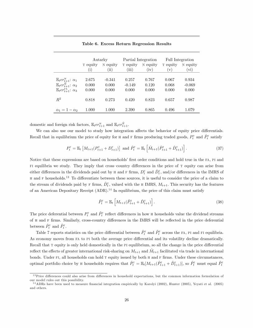
Table 6. Excess Return Regression Results

Autarky Partial Integration Full Integrationt equity n equity t equity n equity t equity n equity(i) (ii) (iii) (iv) (v) (vi)

Eterwt+1: α1 2.675 -0.341 0.257 0.767 0.067 0.934Eterwt+1: α2 0.000 0.000 -0.149 0.120 0.068 -0.069Eterfxt+1: α3 0.000 0.000 0.000 0.000 0.000 0.000

R2 0.818 0.273 0.420 0.823 0.657 0.987

α1 = 1− α2 1.000 1.000 2.390 0.865 0.496 1.079

domestic and foreign risk factors, Eterwt+1 and Eterwt+1.We can also use our model to study how integration affects the behavior of equity price differentials.

Recall that in equilibrium the price of equity for h and f firms producing traded goods, P tt and P tt satisfy

P tt = Et£Mt+1(P

tt+1 +Dt

t+1)¤and P tt = Et

hMt+1(P

tt+1 + Dt

t+1)i. (37)

Notice that these expressions are based on households’ first order conditions and hold true in the fa, pi and

fi equilibria we study. They imply that cross—country differences in the price of t equity can arise from

either differences in the dividends paid out by h and f firms, Dtt and Dt

t , and/or differences in the IMRS of

h and f households.13 To differentiate between these sources, it is useful to consider the price of a claim to

the stream of dividends paid by f firms, Dtt , valued with the h IMRS, Mt+1. This security has the features

of an American Depositary Receipt (ADR).14 In equilibrium, the price of this claim must satisfy

P tt = EthMt+1(P

tt+1 + Dt

t+1)i. (38)

The price deferential between P tt and P tt reflect differences in how h households value the dividend streams

of h and f firms. Similarly, cross-country differences in the IMRS will be reflected in the price deferential

between P tt and P tt .

Table 7 reports statistics on the price differential between P tt and P tt across the fa, pi and fi equilibria.

As economy moves from fa to pi both the average price differential and its volatility decline dramatically.

Recall that t equity is only held domestically in the pi equilibrium, so all the change in the price differential

reflect the effects of greater international risk-sharing onMt+1 and Mt+1 facilitated via trade in international

bonds. Under fi, all households can hold t equity issued by both h and f firms. Under these circumstances,

optimal portfolio choice by h households requires that P tt = Et[Mt+1(Ptt+1 + Dt

t+1)], so Ptt must equal P

tt

13Price differences could also arise from differences in household expectations, but the common information formulation ofour model rules out this possibility.14ADRs have been used to measure financial integration empirically by Karolyi (2002), Hunter (2005), Yeyati et al. (2005)

and others.

26

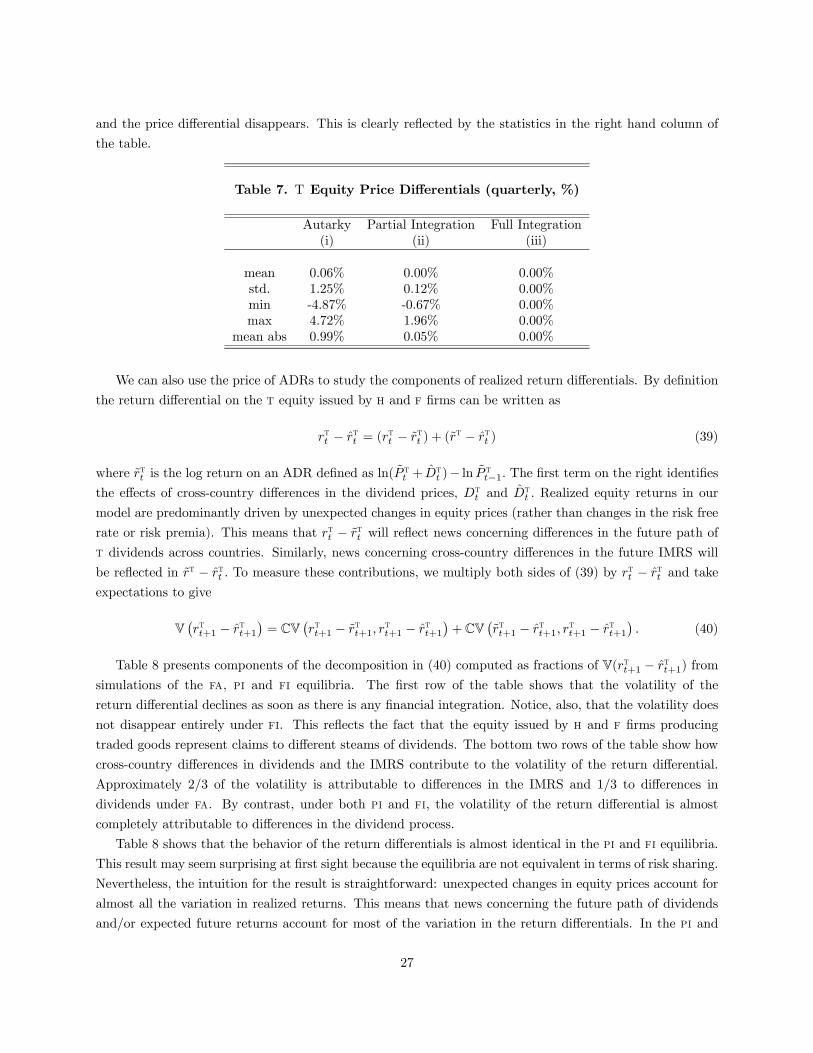
and the price differential disappears. This is clearly reflected by the statistics in the right hand column of

the table.

Table 7. T Equity Price Differentials (quarterly, %)

Autarky Partial Integration Full Integration(i) (ii) (iii)

mean 0.06% 0.00% 0.00%std. 1.25% 0.12% 0.00%min -4.87% -0.67% 0.00%max 4.72% 1.96% 0.00%

mean abs 0.99% 0.05% 0.00%

We can also use the price of ADRs to study the components of realized return differentials. By definition

the return differential on the t equity issued by h and f firms can be written as

rtt − rtt = (rtt − rtt ) + (r

t − rtt ) (39)

where rtt is the log return on an ADR defined as ln(Ptt + Dt

t )− ln P tt−1. The first term on the right identifies

the effects of cross-country differences in the dividend prices, Dtt and Dt

t . Realized equity returns in our

model are predominantly driven by unexpected changes in equity prices (rather than changes in the risk free

rate or risk premia). This means that rtt − rtt will reflect news concerning differences in the future path of

t dividends across countries. Similarly, news concerning cross-country differences in the future IMRS will

be reflected in rt − rtt . To measure these contributions, we multiply both sides of (39) by rtt − rtt and take

expectations to give

V¡rtt+1 − rtt+1

¢= CV

¡rtt+1 − rtt+1, r

tt+1 − rtt+1

¢+CV

¡rtt+1 − rtt+1, r

tt+1 − rtt+1

¢. (40)

Table 8 presents components of the decomposition in (40) computed as fractions of V(rtt+1 − rtt+1) from

simulations of the fa, pi and fi equilibria. The first row of the table shows that the volatility of the

return differential declines as soon as there is any financial integration. Notice, also, that the volatility does

not disappear entirely under fi. This reflects the fact that the equity issued by h and f firms producing

traded goods represent claims to different steams of dividends. The bottom two rows of the table show how

cross-country differences in dividends and the IMRS contribute to the volatility of the return differential.

Approximately 2/3 of the volatility is attributable to differences in the IMRS and 1/3 to differences in

dividends under fa. By contrast, under both pi and fi, the volatility of the return differential is almost

completely attributable to differences in the dividend process.

Table 8 shows that the behavior of the return differentials is almost identical in the pi and fi equilibria.

This result may seem surprising at first sight because the equilibria are not equivalent in terms of risk sharing.

Nevertheless, the intuition for the result is straightforward: unexpected changes in equity prices account for

almost all the variation in realized returns. This means that news concerning the future path of dividends

and/or expected future returns account for most of the variation in the return differentials. In the pi and

27

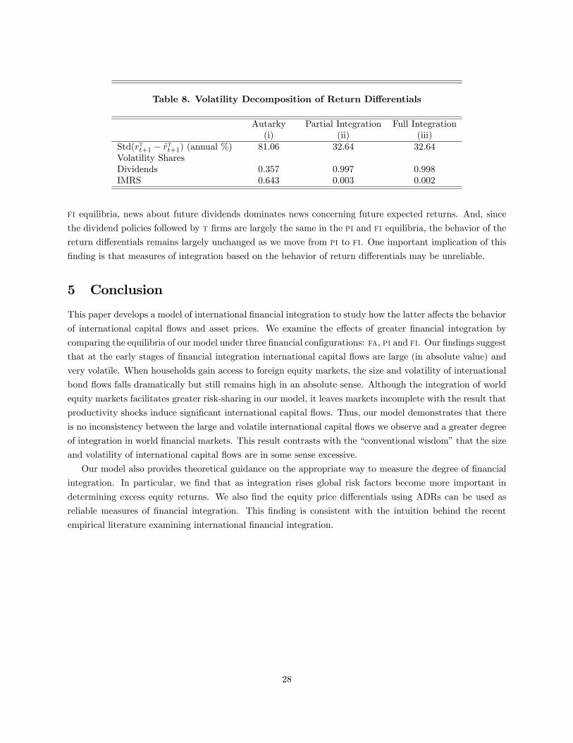
Table 8. Volatility Decomposition of Return Differentials

Autarky Partial Integration Full Integration(i) (ii) (iii)

Std(rtt+1 − rtt+1) (annual %) 81.06 32.64 32.64Volatility SharesDividends 0.357 0.997 0.998IMRS 0.643 0.003 0.002

fi equilibria, news about future dividends dominates news concerning future expected returns. And, since

the dividend policies followed by t firms are largely the same in the pi and fi equilibria, the behavior of the

return differentials remains largely unchanged as we move from pi to fi. One important implication of this

finding is that measures of integration based on the behavior of return differentials may be unreliable.

5 Conclusion

This paper develops a model of international financial integration to study how the latter affects the behavior

of international capital flows and asset prices. We examine the effects of greater financial integration by

comparing the equilibria of our model under three financial configurations: fa, pi and fi. Our findings suggest

that at the early stages of financial integration international capital flows are large (in absolute value) and

very volatile. When households gain access to foreign equity markets, the size and volatility of international

bond flows falls dramatically but still remains high in an absolute sense. Although the integration of world

equity markets facilitates greater risk-sharing in our model, it leaves markets incomplete with the result that

productivity shocks induce significant international capital flows. Thus, our model demonstrates that there

is no inconsistency between the large and volatile international capital flows we observe and a greater degree

of integration in world financial markets. This result contrasts with the “conventional wisdom” that the size

and volatility of international capital flows are in some sense excessive.

Our model also provides theoretical guidance on the appropriate way to measure the degree of financial

integration. In particular, we find that as integration rises global risk factors become more important in

determining excess equity returns. We also find the equity price differentials using ADRs can be used as

reliable measures of financial integration. This finding is consistent with the intuition behind the recent

empirical literature examining international financial integration.

28

References

[1] Adjaoute, Kpate and Jean-Pierre Danthine (2002). ”European Financial Integration and Equity Re-

turns: A Theory-Based Assessment”, European Central Bank.

[2] Albuquerque, Rui, Norman Loayza, and Luis Serven (2003). ”World Market Integration Through the

Lens of Foreign Direct Investors”.

[3] Ayuso, Juan and Roberto Blanco (1999). ”Has Financial Market Integration Increased During The

Nineties?” Banco de España Working Paper 9923.

[4] Bacchetta, Philippe and Eric van Wincoop (1998). ”Capital Flows to Emerging Markets: Liberalization,

Overshooting, and Volatility”, NBER Working Paper No. 6530.

[5] Backus, Dave and Gregory Smith (1993). “Consumption and Real Exchange Rates in Dynamic Exchange

Economies with Nontraded Goods”, Journal of International Economics, Vol. 35, pp. 297-316.

[6] Baele, Lieven, Annalisa Ferrando, Peter Hördahl, Elizaveta Krylova, and Cyril Monnet ”Measuring

Financial Integration in The Euro Area” ECB Occasional Paper Series No. 14.

[7] Baxter, Marianne and Mario J. Crucini (1995). ”Business Cycles and the Asset Structure of Foreign

Trade”, International Economic Review, Vol. 36, pp. 821-854.

[8] _______, Urban J. Jermann, and Robert G. King (1998). ”Nontraded Goods, Nontraded Factors

and International Non-diversification”, Journal of International Economics Vol. 44, pp. 211-229.

[9] Bekaert, Geert and Campbell R. Harvey (1995). ”Time-Varying World Market Integration” The Journal

of Finance, Vol. 50, No. 2, pp. 403-444.

[10] _______ (1997). ”Emerging Equity Market Volatility” Journal of Financial Economics Vol. 43, pp.

29-77.

[11] _______ (2000). ”Capital flows and the behavior of emerging market equity returns”. In: Edwards,

S. (Ed.), Capital Inflows and the Emerging Economies. University of Chicago Press and NBER, Cam-

bridge, MA, pp. 159-194.

[12] _______, and Robin L. Lumsdaine (2002a). ”The Dynamics of Emerging Market Equity Flows”,

Journal of Money and Finance, Vol. 21, pp. 295-350.

[13] _______ (2002b). ”Dating the Integration of World Equity Markets”, Journal of Financial Eco-

nomics Vol. 65, pp.203-247.

[14] Bohn, Henning and Linda L. Tesar (1996). ”U.S. Investment in Foreign Markets: Portfolio Rebalancing

or Return Chasing?”, The American Economic Review, Vol. 86, No. 2, Papers and Proceedings, pp.

77-81.

[15] Brandt, Michael W., Amit Goyal, and Pedro Santa-Clara (2001). ”Dynamic Portfolio Choice: A Simu-

lation Approach”, Anderson Graduate School of Management Finance Paper No. 4-01.

29

[16] Buch, Claudia M., Jorg Dopke, and Christian Pierdzioch (2002). ”Financial Openness and Business

Cycle Volatility”, Kiel Working Paper No. 1121.

[17] ______ and Christian Pierdzioch (2003). ”The Integration of Imperfect Financial Markets: Implica-

tions for Business Cycle Volatility”, Kiel Working Paper No. 1161.

[18] Carrieri, Francesca, Vihang Errunza, and Ked Hogan (2003). ”Characterizing World Market Integration

Through Time” McGill University.

[19] Chan, K.C., G. Andrew Karolyi, and Renl M. Stulz (1992). ”Global Financial Markets and the Risk

Premium on U.S. Equity” Journal of Financial Economics Vol. 32, pp.137-167.

[20] Chen, Zhiwu and Peter J. Knez (1995). ”Measurement of Market Integration and Arbitrage” The Review

of Financial Studies Vol. 8, No. 2, pp. 287-325.

[21] Cochrane, John H. (2001). ”Asset Pricing”, Princeton University Press, Princeton, New Jersey.

[22] Corsetti, Giancarlo, Luca Dedola and Sylvain Leduc (2003). ”International Risk-Sharing and the Trans-

mission of Productivity Shocks”.

[23] Campbell, John Y., Yeung Lewis Chan, and Luis M. Viceira (2000). ”A Multivariate Model of Strategic

Asset Allocation”.

[24] Danthine, Jean-Pierre and John B. Donaldson (1994). ”Asset Pricing Implications of Real Market

Frictions”.

[25] Diermeier, Jeff and Bruno Solnik (2000). ”Global Pricing of Equity”.

[26] Dumas, Bernard and Bruno Solnik (1995). ”The World Price of Foreign Exchange Risk” The Journal

of Finance Vol. 50, No. 2, pp. 445-479.

[27] Engel, Charles and Akito Matsumoto (2004). ”Home Bias in Equities under New Open Economy Macro-

economics”.

[28] Evans, Martin D. D. and Viktoria V. Hnatkovska (2005). ”Approximation Methods for Solving General

Equilibrium Models with Incomplete Markets and Many Assets”.

[29] ______ and Richard K. Lyons (2004), “A New Micro Model of Exchange Rate Dynamics”, NBER

Working Paper No.10379.

[30] Errunza, Vihang and Etienue Losq (1985). ”International Asset Pricing under Mild Segmentation: The-

ory and Test”, The Journal of Finance Vol. 40, No. 1, pp. 105-124.

[31] ______, and Prasad Padmanabhan (1992). ”Tests of Integration, Mild Segmentation and Segmen-

tation Hyposeses”, Journal of Banking and Finance, Vol. 16, pp. 949-972.

[32] Ferson, Wayne E. and Campbell R. Harvey (1993). ”The Risk and Predictability of International Equity

Returns”, The Review of Financial Studies Vol. 6, No. 3, pp. 527-566.

30

[33] Flood, Robert P. and Andrew K. Rose ”Financial Integration: A New Methodology and an Illustration”

http://faculty.haas.berkeley.edu/arose.

[34] Fratzscher, Marcel (2001) ”Financial Market Integration In Europe: On The Effects Of EMU On Stock

Markets” ECB Working Paper No. 48.

[35] Froot, Kenneth A., Paul G. J. O’Connell and Mark S. Seasholes (1998). ”The Portfrolio Flows of

International Investors”, NBER Working Paper No. 6687.

[36] Froot, Kenneth A. and Melvyn Teo (2004). ”Equity Style Returns and Institutional Investor Flows,

NBER Working Paper 10355.

[37] Griffin, John M. and G. Andrew Karolyi (1998). ”Another Look at the Role of the Industrial Structure

of Markets for International Diversification Strategies” Journal of Financial Economics Vol. 50 pp.

351-373.

[38] Hardouvelis, Gikas, Dimitrios Malliaropulos, and Richard Priestley (2000). ”EMU and European Stock

Market Integration” CEPR Discussion Paper No. 2124.

[39] Hau, Harald and Helene Rey (2004a). ”Exchange Rates, Equity Prices and Capital Flows”.

[40] ______ (2004b). ”Can Portfolio Rebalancing Explain the Dynamics of Equity Returns, Equity Flows,

and Exchange Rates?”.

[41] Heathcote, Jonathan and Fabrizio Perri (2002). ”Financial Autarky and International Business Cycles”,

Journal of Monetary Economics Vol. 49, pp. 601-627.

[42] ______ (2004). ”Financial Globalization and Real Regionalization”, Journal of Economic Theory,

Vol.119, No.1, pp. 207-243.

[43] ______ (2004). ”The International Diversification Puzzle is Not as Bad as You Think”, Georgetown

University Working Paper.

[44] Henry, Peter Blair (2000). ”Stock Market Liberalization, Economic Reform, and Emerging Market

Equity Prices” The Journal of Finance Vol. 55, No.2, pp. 529-564.

[45] Heston, Steven L. and K. Geert Rouwenhorst (1994). ”Does Industrial Structure Explain the Benefits

of International Diversification?” Journal of Financial Economics Vol. 36, pp. 3-27.

[46] ______, and Roberto E. Wessels (1995). ”The Structure of International Stock Returns and the

Integration of Capital Markets”, Journal of Empirical Finance Vol. 2, pp. 173-197.

[47] Hunter, Delroy M. (2005). ”What Drives Time Variation in Emerging Market Segmentation”, The

Journal of Financial Research Vol. 28, No. 2, pp. 261-280.

[48] Karolyi, Andrew G. (2002). ”The Role of ADRs in the Development and Integration of Emerging Equity

Markets”, Ohio State University.

31

[49] ______ and Rene M. Stulz (2001). ”Are International Assets Priced Locally or Globally?” Handbook

of the Economics of Finance, George Constantinides, Milton Harris, and Rene M. Stulz, eds., North-

Holland.

[50] Korajczyk, Robert A. and Claude J. Viallet (1989). ”An Empirical Investigation of International Asset

Pricing”, The Review of Financial Studies Vol. 2, No. 4, pp. 553-585.

[51] Kollmann, Robert, (1995). “Consumption, real exchange rates and the structure of international asset

markets”, Journal of International Money and Finance, 14, pp. 191- 211.

[52] Kose, M. Ayhan, Eswar S. Prasad, and Marco E. Terrones (2003). ”Financial Integration and Macro-

economic Volatility”, IMF Working Paper WP/03/50.

[53] Lessard, Donald R. ”World, National, and Industry Factors in Equity Returns”, The Journal of Finance,

Vol. 29, No. 2, Papers and Proceedings of the Thirty-Second Annual Meeting of the American Finance

Association, New York, New York, pp. 379-391.

[54] Markowitz, Harry (1952). ”Portfolio Selection”, The Journal of Finance, Vol 7, No. 1, pp. 77-91.

[55] Martin, Philippe and Helene Rey (2000). ”Financial Integration and Asset Returns”.

[56] Merton, Robert C. (1969). ”Lifetime Portfolio Selection under Uncertainty: The Continuous-Time

Case”, The Review of Economics and Statistics Vol. 51, No.3, pp. 247-257.

[57] Lewis, Karen K. (1999). ”Trying to Explain Home Bias in Equities and Consumption”, Journal of

Economic Literature Vol.37, pp. 571-608.

[58] Obstfeld, Maurice (1994). ”Risk-Taking, Global Diversification, and Growth”, The American Economic

Review, Vol. 84, No. 5, pp. 1310-1329.

[59] ______ and Kenneth Rogoff (1996). ”Foundations of International Macroeconomics”, The MIT

Press, Cambridge, Massachusetts.

[60] Pesenti, Paolo and Eric van Wincoop (1996). ”Do Nontraded Goods Explain the Home Bias Puzzle?”,

NBER Working Paper No. 5784.

[61] Rouwenhorst, K.Geert (1999). ”European Equity Markets and the EMU”, Financial Analysts Journal,

pp.57-64.

[62] Samuelson, Paul A. (1969). ”Lifetime Portfolio Selection by Dynamic Stochastic Programming”, The

Review of Economics and Statistics Vol. 51, No.3, pp. 239-246.

[63] Senay, Ozge (1998). ”The Effects of Goods and Financial Market Integration on Macroeconomic Volatil-

ity”, The Manchester School.

[64] Serrat, Angel (2001). ”A Dynamic Model of International Portfolio Holdings”, Econometrica, Vol. 69,

No. 6, pp. 1467-1489.

32

[65] Smith, P. N., Sorenson S., and M. R. Wickens (2003). ”An Asset Market Integration Test Based on

Observable Macroeoconomic Stochastic Discount Factors”, University of York.

[66] Stockman, C. Alan and Linda L. Tesar (1995). ”Tastes and Technology in a Two-Country Model of the

Business Cycle: Explaining International Comovements”, The American Economic Review, Vol. 85 (1),

pp. 168-185.

[67] Stulz, Rene M. (1999). ”International Portfolio Flows and Security Markets”, Working Paper.

[68] Sutherland, Alan (1996). ”Financial Market Integration and Macroeconomic Volatility”, Scandinavian

Journal of Economics, Vol. 98 (4), pp. 521-539.

[69] Tesar, Linda L. (1993). ”International Risk Sharing and nontraded Goods”, Journal of International

Economics, Vol. 35, pp. 69-89.

[70] Yeyati, Eduardo Levy, Sergio L. Schmukler, and Neeltje Van Horen (2005). ”International Financial

Integration through the Law of One Price”, Universidad Torcuato di Tella.

33

A Appendix: Approximations

This appendix describes the approximations used in the solution of the model. A formal discussion of the

solution technique is presented in Evans and Hnatkovska (2005).

In our model the equilibrium conditions include equations (6), (7) and (19a)-(19e) characterizing house-

hold’s behavior, equations (24) describing firm’s problem at h country, a symmetric system of conditions

for the f country, a set of market clearing conditions in equations (10)-(12) and (16)-(18b), plus return

definitions in (20)-(22). The system in summarized below.

Rwt+1 = Rt + αtt¡Rtt+1 −Rt

¢+ αtt

³Rtt+1 −Rt

´+ αnt

¡Rnt+1 −Rt

¢,

Wt+1 = Rwt+1 (Wt − Ctt −QntCnt ) ,

Qnt =

µλnλt

¶1−φµCntCtt

¶φ−1, (A1)

1 = Et [Mt+1Rt] ,

1 = Et£Mt+1R

tt+1

¤,

1 = EthMt+1R

tt+1

i,

1 = Et£Mt+1R

nt+1

¤,

Mt+1 = β

µCtt +QntC

nt

Ctt+1 +Qnt+1Cnt+1

¶, (A2)

Ktt+1 = (1− δ)Kt

t + ezttKtθ

t −Dtt ,

1 = EthMt+1

³θZtt+1 (Kt+1)

θ−1+ (1− δ)

´i,

Cnt = Y nt = Dn

t ,

Ctt + Ctt = Y tt + Y t

t − It − It,

1 = Att + Att ,

1 = Ant ,

Bt + Bt = 0,

An analogous set of conditions for foreign country applies. To solve the model, we first find its non-

stochastic steady state. The system of equilibrium equations is then log-linearized as follows. The equations

pertinent to the real side of the model are log-linearized up to the first order, while those related to the

financial side - up to the second order. Real variables, such as capital, dividends, etc. are stationary around

their steady state. Individual’s financial wealth is linearized around its initial distribution. Distributions of

consumption and portfolio shares will be pinned down endogenously by the model. All small letters denote

log transformation of the corresponding variable, measured as deviation from the steady state or its initial

level.

The log return on h wealth can be approximated as

rwt+1 = rt +α0tert+1 +1

2α0t¡σ2t − Σtαt

¢. (A3)

CCV show that this approximation holds exactly in continuous time and remains a good approximation in

A1

discrete formulation with short time intervals.

The budget constraint of the h household in (6) can be simplified when preferences are logarithmic. In

particular, the optimal consumption-wealth ratio under log-utility preferences is constant and is equal to

(1− β) so Ctt +QntCnt = (1− β)Wt. The simplified budget constraint then becomes

Wt+1 = Rwt+1 (Wt − Ctt −QntCnt ) = βRwt+1Wt,

whose log-linearized form is

∆wt+1 = rwt+1 + lnβ. (A4)

Next, we turn to the IMRS. By definition,

Mt+1 =β¡∂U/∂Ctt+1

¢(∂U/∂Ctt )

= β

µCtt +QntC

nt

Ctt+1 +Qnt+1Cnt+1

¶,

which can be simplified further with log preferences to

Mt+1 = βWt

Wt+1,

or in logs

mt+1 = −∆wt+1 + lnβ.

The Euler equations are linearized using a second-order Taylor series expansion and lognormality of asset

returns. We start with the consumption Euler equation in (19a):

1 = Et [exp(mt+1 + rt)] ' exp£Et (mt+1 + rt) +

12Vt (mt+1)

¤.

Taking logs on both side yields a log-linearized Euler equation for the international bond:

0 = rt + Etmt+1 +12Vt (mt+1) . (A5)

The equity Euler equations are log-linearized analogously:

1 = Et£Mt+1R

χt+1

¤' exp

£Et¡mt+1 + rχt+1

¢+ 1

2Vt¡mt+1 + rχt+1

¢¤.

Again, taking logs and substituting in the bond Euler equation gives equation (30):

Etrχt+1 − rt +12Vt

¡rχt+1

¢= −CVt

¡mt+1, r

χt+1

¢. (A6)

The system (19b)-(19e) can be summarized is terms of portfolio shares αt and first and second moments

of asset returns as

Etert+1 = Σtαt − 12σ

2t . (A7)

A2

Using this equation, the budget constraint in (A4) can be rewritten as:

∆wt+1 = rt +12α

0tΣtαt +α0t (ert+1 − Etert+1) . (A8)

The optimal dividend policy of domestic firm implies

1 = EthMt+1

³θZtt+1 (Kt+1)

θ−1+ (1− δ)

´i.

Again, we apply the log-normal approximation to get

Etrkt+1 − rt +12Vt

¡rkt+1

¢= −CVt

¡mt+1, r

kt+1

¢, (A9)

where rkt+1 = ψztt+1 − (1− θ)ψkt+1 and ψ = 1− β (1− δ) .

Next, we turn to the market clearing conditions. Bond market clearing from (16) requires Bt + Bt = 0.

Substituting for bonds from (26) into this condition gives

β³Wt + Wt

´=³P tt + P tt

´+³QntP

nt + Qnt P

nt

´.

In addition, since each aggregate consumption is a constant fraction of wealth, the same relation holds at

the global level

(1− β)³Wt + Wt

´=³Ctt + Ctt

´+³QntC

nt + Qnt C

nt

´.

Combining the last two equations gives

(1− β)h³P tt + P tt

´+³QntP

nt + Qnt P

nt

´i= β

h³Ctt + Ctt

´+³QntC

nt + Qnt C

nt

´i.

The linearized version of this expression isnP tptt + P tptt +QnP n (qnt + pnt ) + QnP n (qnt + pnt )

o³P t + P t

´+³QnP n + QnP n

´=

nDtdtt + Dtdtt +QnDn (qnt + dnt ) + QnDn

³qnt + dnt

´o³Dt + Dt

´+³QnDn + QnDn

´ , (A10)

where we have also applied the t and n goods market clearing conditions.

Market clearing in the t equity market requires 1 = Att + Att . Substituting for Att and Att in terms of

portfolio shares αt from (26) we obtain

exp (ptt − wt − lnβ) = αtt + αtt · exp (wt − wt) .

Approximation of the exponential terms on both sides is done around the aggregate steady state share of

t equity issued in h country, αt = αt + αt. With the benchmark symmetric parametrization this share is

equal to half of h country wealth. The other half is allocated into n equity. This split is determined by

A3

the preference parameters on t and n consumptions and the assumption about equal initial distribution of

wealth across countries. So, we get

P t

βW+

P t

βW(ptt − wt) +

12

P t

βW(ptt − wt)

2= αtt + αtt

ÃW

W+

W

W(wt − wt) +

12

W

W(wt − wt)

2

!,

which becomes

αt³1 + (ptt − wt) +

12 (p

tt − wt)

2´= αtt + αtt

³1 + (wt − wt) +

12 (wt − wt)

2´. (A11)

The approximation for the f country t equity market clearing is symmetric and is approximated around the

aggregate steady state share of t equity issued by the foreign country, αt = αt + αt :

αt³1 + (ptt − wt) +

12 (p

tt − wt)

2´= αtt + αtt

³1 + (wt − wt) +

12 (wt − wt)

2´. (A12)

In summary, the system of linearized equations used to characterize the equilibrium in full integration

model consists of:

• the productivity process in (4);

• the three Euler equations for equity as given by equation (A6) for χ = t,t,n in each country;

• the Euler equation for capital, given in (A9) for each country;

• the budget constraint in each country as given in equation (A8);

• t goods market clearingctt + ctt = dtt + dtt ;

• bond market clearing reformulated in terms of dividends and prices in (A10);

• t equity market clearing as derived in (A11)-(A12);

• n equity definition from equation (26)

αnt = αnµ1 + (qnt + pnt − wt) +

1

2(qnt + pnt − wt)

2

¶(A13)

αnt = αnµ1 + (qnt + pnt − wt) +

1

2(qnt + pnt − wt)

2

¶.

B Appendix: Robustness

Varying the initial wealth distribution In order to solve the model we need to make an assumption

about the initial distribution of wealth across the countries. The results in the text assume that both

countries have identical wealth to start with. To check the robustness of our results, we considered an

alternative solution to the model based on the relative wealth of country f to h equal to 1.00218. This wealth

A4

distribution implies an initial current account deficit for country h equal to 4% of GDP. Re—solving the model

with this initial wealth distribution (and the other model parameters unchanged) does not materially affect

the model solution. In particular, the dynamics of international capital flows and returns are similar to those

we report in the text.

Varying the weight assigned to n consumption Our benchmark model parametrization also assumes

that two countries are perfectly symmetric in terms of preferences, production and shocks. As a result, the

model predicts that investors take fully diversified positions in t equity shares. This prediction is, however,

at odds with the persistent equity home bias observed in the actual portfolio holdings of most developed

countries. Our next robustness exercise, therefore, consists of studying the effects of integration on capital

flow dynamics in the presence of home bias in equity portfolios. We accomplish this by biasing preferences of

consumers towards n consumption in their aggregate basket. In particular, we assume that share parameters

λn and λn in the utility function increase to 0.75.

We find that when households put more weight on n consumption in their utility function, they also

increase the share of their wealth allocated into equity providing claims to n consumption, thus leading to

the home bias in aggregate domestic portfolios. In particular, the average n equity share in both h and f

countries is equal to 81.53% under the new parametrization. The remaining wealth is allocated into t equity,

which, under fi is equally split between h and f issued claims. As a result, even though the model generates

home bias through an increase in the share of n equity, the t equity holdings remain fully diversified.

The degree of risk sharing under fi is smaller in this version of the model: the cross—country correlation

in log IMRS is now 0.562 rather than 0.669. The size and volatility of both bond and equity flows are higher

than in our benchmark case, under fi. By contrast, the size and volatility of bond flows under pi remain

much the same. Overall, our finding of a hump-shaped relation between capital flows and the degree of

integration, appears robust.

A5