1

Internal Condensing Flows inside a Vertical Pipe –

Experimental/Computational Investigations of the Effects of Specified and

Unspecified (Free) Conditions at Exit

A. Narain1, J. H. Kurita, M. Kivisalu, A. Siemionko, S. Kulkarni, T. W. Ng, N. Kim, and L. Phan

Department of Mechanical Engineering-Engineering Mechanics

Michigan Technological University

Houghton, MI-49931

ABSTRACT

Reported experimental and computational results confirm that both the flow features and heat transfer rates inside a

condenser depend on the specification of inlet, wall, and exit conditions. The results show that the commonly occuring

condensing flows’ special sensitivity to changes in exit conditions (i.e. changes in exit pressure) arise from the ease with

which these changes alter the vapor flow field in the interior. When exit pressure is changed from one steady value to

another, the changes required of the interior vapor flow towards achieving a new steady flow are such that they do not

demand removal of the new exit pressure imposition back to the original steady value - as is the case for incompressible

single phase flows with an original and “required” exit pressure. Instead, new steady flows may be achieved through

appropriate changes in the vapor/liquid interfacial configurations and associated changes in interfacial mass, heat transfer

rates (both local and overall), and other flow variables. This special feature of these fows is for the commonly occurring

large heat sink situations for which the condensing surface temperature (not heat flux) remain approximately the same for

any given set of inlet conditions while exit condition changes. In this paper’s context of flows of a pure vapor that

experience film condensation on the inside walls of a vertical tube, the reported results provide important quantitative and

qualitative understanding as well as exit-condition based categorization of the flows.

Experimental results and selected relevant computational results that are presented here reinforce the fact that there

exist multiple steady solutions (with different heat transfer rates) for multiple steady prescriptions of the exit-condition –

even though the other boundary conditions do not change. However for some situations that do not fix any specific value for

the exit condition (say exit pressure) but allow the flow the freedom to choose any exit pressure value within a certain

range, experiments confirm the computational results that, given enough time, there typically exists, under normal gravity

conditions, a self selected “natural” steady flow with a “natural” exit condition. This happens if the vapor flow is seeking

(or attracted to) a specific exit condition and the conditions downstream of the condenser allow the vapor flow a range of

exit conditions that includes the specific “natural” exit condition of choice. However, for some unspecified exit condition

cases involving partial condensation, even if computations predict that a “natural” exit condition choice exists, the

experimental arrangement employed here does not allow the flow to approach its steady “natural” exit condition value and,

instead, it only allows oscillatory exit conditions leading to an oscillatory flow. For the reported experiments, these

oscillatory pressures are induced and imposed by the instabilities in the system components downstream of the condenser.

Key-words: film condensation, phase-change heat transfer, two-phase flows, interfacial waves.

1To whom correspondence should be addressed.

E-mail: narain@mtu.edu, Phone: 906-487-2555

Fax: 906-487-2822

2

NOMENCLATURE

D Inner diameter of the test-section, m

G Inlet mass flux, kg/(m2/s)

hfg(p) Heat of vaporization at pressure p, J/kg

h Average convective heat coefficient, W/(m2-K)

Ja Condensate liquid Jacob number

L Length of the test-section, m

inM⋅

Vapor flow rate at test-section inlet, g/s

LM⋅

Liquid flow rate at test-section exit, g/s

VM⋅

Vapor flow rate at test-section exit, g/s

pb Evaporator (boiler) pressure, kPa

pD2 Pressure at the location near the rotameter, kPa

pT" Pressure at the location outside the test section, kPa

pin Pressure at location at the test-section inlet, kPa

pexit Pressure at location at the test-section exit, kPa

Pr1 Condensate liquid Prandtl number.

pxi Test-section pressures at different locations x = xi (i = 1, 2, …), kPa

q ′′′′′′′′ Average convective heat flux, W/m2

bQ⋅

Net heat rate into the evaporator, W

outQ⋅

Net heat rate out of the test-section, W

Re Inlet vapor Reynolds number

Tb Evaporator temperature, oC

TR Rotameter temperature, oC

Tsat(p) Saturation temperature at pressure p, oC

Ts-xi Condensing surface temperatures at different locations x = xi (i = 1, 2, …), oC

wT Mean uniform condensing surface temperature, oC

Tw (x) Non-uniform steady condensing surface temperature, oC

TV-in Vapor temperature at test-section inlet, oC

TC-in Temperature of the counter-current coolant water flow at the approach to the test-section, oC

Xfc Approximate length needed for full condensation (estimted by computations), m.

3

xe Ratio of test section length to test section inner diameter (L/D).

T∆ Tsat(p) - wT , oC

∆Tsup Vapor superheat, TV-in - Tsat(p) , o

C

∆p pin – pexit, kPa

Ze Ratio of exit vapor flow rate to total inlet flow rate

Ze-expt Ze as obtained by experiments

Ze-comp Ze as obtained by computations

ρ 2 Density of vapor, kg/m3

ρ1 Density of liquid, kg/m3

µ2 Viscosity of vapor, kg/(m-sec)

µ1 Viscosity of liquid, kg/(m-sec)

Subscripts

exit Test-section exit

in Test-section inlet

Na Natural steady case

1. INTRODUCTION

This paper outlines a fundamental and novel experimental investigation of effects of exit

conditions on internal condensing flows. Reported experimental results confirm the existing

computational results ([1], [2], [3]) that both the flow features and heat transfer rates inside a condenser

are sensitive to exit conditions and therefore depend on the specification of inlet, wall (particularly

condensing surface temperature), and exit conditions. The condensing surface temperature (not heat

flux) is assumed known (and fixed) or knowable (through consideration of approriate conjugate

problem). This is true because, geneally, heat is removed from the condensing flow through a wall and

put in a large heat sink which may be a steady coolant flow in contact with the other side of the wall-

surface or a suitabe arrangement of thermo-electric coolers. The paper identifies and establishes

4

multiplicity of steady/quasi-steady solutions – and/or oscillatory flows – under different conditions at

the exit. Experiments support the existing simulation results ([1], [2], [3]) that have already shown the

presence of different steady/quasi-steady solutions for different steady specifications of the exit

condition. Exit condition for condenser is specified by exit pressure. For partial (incomplete)

condensation flows, specification of exit pressure is equivalent (see Fig. 6 in [1]) to specification of

exit vapor quality (the ratio of vapor mass flow rate at the exit to the inlet mass flow rate). The

computational simulations ([1], [2], [3]) for the gravity driven partial condensation cases inside a

vertical tube predict that, for a certain set of inlet and wall conditions, even if the exit condition is not

specified and a suitable range of exit conditions is available for the flow to choose from, the flow seeks

and attains a specific “natural” exit condition (in Narain et al. [1] this situation is also termed natural

unspecified steady exit condition due to the presence of an “attractor”, i.e., an attracting solution).

Unfortunately many planned system designs incorporate a condenser and assume that the condenser

will always attain a steady flow even if no exit conditions are specified. This is not generally true. The

attainment of steady flows under unspecified exit conditions occur more readily (over a larger

parameter zone) for gravity driven condensate flows as opposed to shear driven flows (see [3]). The

reported experimental results for gravity driven partial condensation cases under unspecified exit

conditions support the computational results – both qualitatively and quantitatively. However the

steady “natural” exit condition may or may not exist depending on whether or not a steady “attractor”

exists (e.g., as shown in [3], it does not exist for most slow inlet flowrates in horizontal or zero gravity

conditions) and even if an “attractor” does exist, its realization depends on whether the attracting

“natural” exit condition value falls within the range of the available steady choices at the exit. In the

absence of active specification of a steady exit condition, the available range of steady exit conditions

is determined by the components downstream of the condenser and the specific nature of the flow loop

design. Furthernore, because of the small pressure drops (see [3] or experimental runs reported here),

5

when a steady “natural” exit condition is achieved under unspecified conditions, or the specified exit

condition is not too far from this “natural” steady exit value, typically, vapor flows are close to

incompressible.

The fact that, for partial condensation flows, one can achieve quite different values of average

heat transfer coeffiecients under different realizations of quasi-steady flows that correspond to different

specifications of exit vapor quality (or pressure) is not surprising - as this follows from a simple overall

energy balance. In the context of boundary value problems for internal condensing flows, what is new

is that our computational and experimental results unequivocally show that the commonly occuring

condensing flows are very sensitive to the nature of exit conditions as well as to the changes in exit

conditions (due to changes in exit pressure). This sensitivity arises from the ease with which these

changes alter the vapor flow field in the interior. Therefore when only exit condition is changed from

one steady value to another, the changes required for the interior vapor flow towards attaining a new

steady flow are such that they do not demand removal of the new exit pressure imposition - as is the

case for incompressible single phase flows with only one allowed exit pressure. Instead, for condensing

flows, new steady flows are achieved for new exit conditions through appropriate changes in the

vapor/liquid interfacial configurations and associated changes in interfacial mass, heat transfer rates

(both local and overall), and other flow variables.

The vertical in-tube internal condensing flows – partial or complete (full) – are investigated

here for downflow configuration. Though numerous in-tube condensation experiments have been done,

most of the well known in-tube vertical downflow experiments done by Goodykoontz and Dorsch [4]-

[5], Carpenter [6], etc. either limit themselves to sufficiently fast flows that do not significantly depend

on exit conditions or operate under a particular set of exit conditions (that automatically gets

determined by the employed experimental set up) and, therefore, results may vary from one

experimental system to another. In addition to our group’s very early (see Yu [7]) and subsequent ([1],

6

[2]) computational findings on the importance of exit conditions for internal condensing flows,

experimental findings of Rabas and Arman ([8]) have also indicated the significance of exit conditions

through their observation that presence or absence of valves at the exit affected some of their in-tube

vertical downflow results. Rabas and Arman [8] also pointed out an important fact that, in the annular

regime, even for complete condensation in a vertically downward flow inside a tube (for which, at exit,

the condensate is collected in a vapor plenum), the condensing flow is usually annular all the way up to

the exit – that is, a continuous liquid phase never fills the entire tube. This ensures that the flow

remains annular (or, at most, has a few liquid bridges that encapsulate vapor bubbles) in the segment

downstream of the point of complete condensation. Beyond this point, average vapor flow rate and

interfacial mass flux remain zero for all practical purposes. Additionally Rabas and Arman [8] have

also pointed out that, in the case of horizontal in-tube complete condensation, the flow regime near the

point of complete condensation (where vapor flow rate is nearly zero) is known to vary from gravity

dominated stratified to gravity dominated plug-annular depending on whether the inlet mass flow rate

is above or below a certain critical value.

Furthermore, on a related topic, several experimental results and analyses ([9] - [17]) indicate

that, for certain physical arrangements leading to a specific class of inlet and outlet conditions,

transients and instabilities are expected in complete condensation internal condensing flows. Since

these experiments and the corresponding modeling techniques in the literature ([9] - [17]) limit

themselves to a particular type of inlet and exit conditions, they do not directly apply to the presence or

absence of observed transients and instabilities in other feasible categories of exit-condition

specifications.

Since understanding of internal condensing flows’ transients is not entirely possible in the

context of traditional two-phase flow analyses based on homogeneous, separated, or drift flux

formulations (see Wallis [18]), more sophisticated averaged model equations of varying degrees of

7

complexities (see, e.g., Lahey and Drew [19]) have been proposed. Despite this, appropriate drift-flux

and/or virtual mass force based analyses of Liao et al. ([20], [21]) and Wang ([22]) report some ability

to capture transients in certain internal condensing flows of the type studied by Wedekind et al.

([9],[12],[15]), Bhatt et al. ([10],[11],[13]), Kobus et al. ([16]-[17]), Boyer et al. [14], etc. Furthermore

Liao et al. ([20],[21]) have also reported difficulties in employing multi-dimensional, four field, two-

fluid model of Lahey and Drew [19] towards modeling transients and instabilities that are observed in

internal condensing flow cases of their concern. Other analyses of Wedekind et al. ([9],[12]), Bhatt et

al. ([10],[11]), and Kobus et al. ([16],[17]) employ the system mean void fraction (SMVF) model

which allows one to ignore the momentum balance equation. These simpler integral analyses have been

somewhat successful in capturing some features of the experimentally observed transients and flow

oscillations that have been reported ([9],[11]) for certain in-tube horizontal condensing flows involving

complete condensation. In these cases, a fixed-pressure tank (plenum) at sufficiently high pressure

pushes vapor through an inlet valve to the inlet of a horizontal condensing section where the vapor is

fully condensed and then the liquid flows out of the condenser exit, through an exit valve, to a fixed -

pressure tank (plenum) at low pressure.

To understand exit condition issues more clearly, the approach taken here has been to seek

experimental confirmation of key results obtained from employing our fundamental and nearly exact

computational technique ([1]-[3]) to obtain steady and unsteady simulations for laminar-vapor/laminar-

condensate initial boundary value problems - in the limited context of separated quasi-steady annular

condensing flows. Therefore, simulation results regarding internal condensing flows’ sensitivity to exit

conditions ([1]-[3]) have been central to the planning and development of the reported experiments and

to the interpretation of the experimental results reported here. Fundamentally, internal condensing

flows’ exit condition sensitivity arises from governing equations being “elliptic” or requiring “two-

way” space co-ordinates in the flow direction (see, e.g., Patankar ([23] or Fig. 1c). However this

8

sensitivity to exit conditions or “two-way” behavior (i.e. flow variable at a point is influenced both by

upstream and downstream local neighbors) is special and does not result from the typical “ellipticity”

associated with slow flows and flow reversals (which are, as described in Patankar [23], associated

with the changes in the sign of local Peclet numbers). In fact, it is found (for simulations in [1]-[3]) that

even when vapor and liquid flows are unidirectional and local Peclet numbers (which appear in local

discretization equations for the velocity components - see eqs. (5.61) – (5.64) in [23]) are very large,

the flows exhibit “elliptic” or “two-way” behavior leading to sensitivity to exit conditions. This special

sensitivity to exit condition is due to “two-way” behavior of the vapor pressure fields (reflected, in the

context of our computational methodology [1], by the “two-way” behavior of the pressure equations

given by eqs. (6.30) – (6.31) in [23]). These equations for condensing flows are such that the

coefficients that multiply the pressures at the locally upstream and downstream neighbors are

comparable even for large Peclet numbers. Due to this, effects of changes in the exit pressure are felt

by the entire vapor flow field that is able to accommodate these changes because of the extra degree of

freedom associated with multiple interface locations and associated heat transfer rates. As a result,

when exit condition is changed from one steady value to another, the changes required for the interior

vapor flow towards attaining a new steady flow are such that they do not demand removal of the new

exit pressure imposition back to the original and “natural” steady value - as is the case for

incompressible single phase flows. In stead, new steady flows are achieved through appropriate

changes in the vapor/liquid interfacial configurations and associated changes in interfacial mass, heat

transfer rates (both local and overall), and other flow variables.

The simulation results ([1]-[3]) supporting the experiments in this paper have already

established that, for partial condensation, conditions at the exit of a condenser can be specified by

unsteady or steady specification of the exit vapor quality (see Fig. 6 in [1]). Equivalently, and, more

generally (for partial and full condensation cases), the exit-condition can be specified by specifying the

9

exit pressure values. The underlying simulations ([3]) and experiments reported here also show that, for

cases where the flow loop does not actively specify any exit condition (as is often the case with many

condenser applications), given enough time, the flow may or may not be able to select a quasi-steady

flow with a “natural” exit condition. This is because the unspecified exit condition cases, though

commonly used in applications, are essentially “ill posed” boundary value problems and therefore

existence of steady solutions are at the mercy of other factors (such as whether or not an “attracting”

steady solution exists and, if it does, whether or not downstream conditions are conducive to the

attainment of this “attracting” solution). Typically, for gravity dominated annular flows of the type

considered here, a “natural” exit condition does exist. In the literature, condensing flows have been

classified as to whether they are shear dominated or gravity dominated, internal or external, smooth or

wavy at the interface, laminar or turbulent in the two phases, etc. It is proposed here that one can only

make sense of the vast literature on internal condensing flows if they are also classified in different

categories based on the conditions imposed at the inlet and the exit. The following three categories

(termed categories I – III) proposed here cover most cases of interest.

Category I (with complete or incomplete condensation under specified exit conditions)

• Prescribed or known values of total inlet mass flow rate (kg/s)Min

& , inlet vapor quality, inlet pressure

pin, and inlet temperature at all times t. Without loss of generality, one can focus on an all vapor

flow (an inlet vapor quality of unity) at the inlet with known values of total inlet (all vapor) mass

flow rate (kg/s)Min

& , inlet pressure pin, and inlet temperature (at saturation temperature Tsat(pin) or at

some superheat) at all times t. This means the prescription could be steady or unsteady.

• Prescribed or known wall temperatures Tw(x,t) < Tsat(pin) for all x-locations over which film

condensation occurs. Typical wall temperature conditions of interest are steady, but unsteady

conditions are relevant to start-up and shutdown.

10

• Prescribed or known exit condition. For example, for steady exit conditions, exit pressure pe =

constant, which is equivalent, for partial condensation cases, to setting exit mass quality

(kg/s)M(kg/s)MZ inVapor@exite&&≡ = an appropriate constant, where (kg/s)M Vapor@exit

& is the vapor

mass flow rate at the exit at time t.

Category II (with complete or incomplete condensation under unspecified exit conditions)

• Prescribed or known values of inlet mass flow rate (kg/s)Min

& , inlet pressure pin, and inlet temperature

(at saturation temperature Tsat(pin) or at some superheat) at all times t. Without loss of generality, it

is assumed that the flow is all vapor at the inlet.

• Prescribed or known wall temperatures Tw(x,t) < Tsat(pin) for all x-locations over which film

condensation occurs.

• No exit condition is prescribed, except for some system hardware limitations that may restrict the

range of exit conditions available to the condenser.

Category III (complete condensation involving special specified conditions at the inlet and the exit)

Though, technically, this is a special form of category I flows, it is listed separately because it

correlates with a different experimental set-up whose choice of hardware facilitate imposition of this

special class of inlet and outlet prescriptions. This class has been extensively investigated in the

literature ([9]-[16]) for oscillatory condensing flows.

• In this case there is a constant pressure reservoir, with a high pressure pTank-in, that feeds the vapor

flow (at inlet pressure pin, temperature TV-in, and density ρV-in) into the test section through an inlet

valve (with valve coefficient ki). This requires that the inlet pressure, pin, satisfy:

in-V

in

iin-Tankin ρ

2(t)Mkpp

&

−≅

11

• Also there is a constant pressure exit tank with a lower pressure pTank-exit to which the condensate

flows through an exit valve of valve coefficient ke. The exit valve handles an all liquid flow

because this case is only for complete condensation flows. At the exit of the condenser, the flow

rate is exit

M& at any time, t, and the liquid density is ρL-exit. This requires that the test section exit

pressure, pexit, satisfy:

exitL

exit

eexitTankexit ρ

2(t)M

kpp−

− +≅&

• Prescribed or known steady wall temperatures Tw(x) < Tsat(pin) for all x-locations over which film

condensation occurs.

In the above context, the experiments and computations in this paper focus only on category I

and category II flows. The reported experiments also define specific flow loop arrangements that allow

realization of flows in these two categories. The experimental and/or modeling analysis papers of

Wedekind et al. ([9],[12]), Bhatt et al. ([10]-[11],[13]), Kobus et al. ([16],[17]), Liao et al. ([18],[19]),

etc. focus on category III flows for a horizontal condenser. Category III flows are not the subject of this

paper. As a result, the flow transients and system instabilities reported in this paper, as far as flows

within the test-section are concerned, are necessarily of different origin. However, at a system level, the

experimentally observed flow oscillations’ relationship to the better known ([11],[13]) results for

category III flows in the downstream auxiliary condenser is discussed here.

The experimental runs reported here largely involve laminar condensate and turbulent vapor

situations with possible vapor compressibility effects. Despite this, both qualitative and quantitative

comparisons with simulation results based on the laminar-vapor/laminar-condensate methodology

given in [1]-[3] are possible, and are presented here, for a feasible subset (within the boundaries for

steady annular flows) of experimental runs. This comparison is possible because turbulent vapor often

12

laminarizes in the vicinity of laminar condensate as the condensate is slow and remains laminar

approximately up to Reδ ≤ 1800 (see film Reynolds number Reδ definition in Phan and Narain [24]).

Also, for gravity driven condensate cases considered here, existence of turbulent vapor zones in the

core and entrance zone of the condenser has only minor second order impact on pressure variations in

the condenser. The far field vapor turbulence often tends not to be a significant player because the

overall flow features (local and average heat transfer coefficients) are dominated by interfacial mass

and heat transfer rates which are dominated by the typically laminar nature of the gravity driven

condensate flow and the associated laminar nature of vapor flow in the vicinity of the interface.

Because of the above, all experimental runs reported here for partial (or incomplete) condensation

cases involving laminar condensate show a very good qualitative agreement with the simulations as far

as existence of multiple steady solutions for multiple steady exit conditions (category I) and a “natural”

steady solution for the unspecified exit condition cases (category II) are concerned. The agreement with

simulations, with regard to exit vapor quality and general consistency with overall heat transfer rates,

are also quantitatively very good for experimental runs that fit the annular flow assumption for the

simulations. It should be noted that, additionally, the accuracy of the employed simulation

methodology ([1] - [3]) and its quantitative compatibility with a different set of experimental runs (Lu

and Suryanarayana [25]) for shear dominated flows (category II) have also been established (see [2]).

Furthermore, computational results for internal condensaing flows are obtained from a simulation tool

that has a proven ability (see Phan and Narain [24]) to make good quantitative predictions for wave

phenomena and their effects on heat transfer rates for the benchmark classical problem of Nusselt [26].

Besides this, since the simulation yields all flow variables including interface locations, it can

potentially be used towards validating/supporting more complex averaged equations (such as Lahey

and Drew ([19]) which would necessarily be needed for more complex flow regimes (dispersed,

bubbly, intermittent plug-slug, etc.).

13

Experimental investigation of annular complete condensation cases reported here are less

complete and limited to “natural” steady flows in category-II. Computational simulations for these

cases are also limited because the flow often condenses completely somewhere within the test-section

and the current simulation technique can only cover the zone from the inlet to the point of full

condensation. The simulation tool has not yet been enhanced to automatically identify and handle the

exit-pressure sensitive adiabatic two-phase annular flow between the point of full condensation and the

exit. The reported experiments cover “natural” full condensation cases under unspecified exit

conditions and the hardware needed to investigate complete condensation category-I flow (i.e.,

prescribed exit condition case) is being developed as an important ongoing area of research.

The exit condition sensitivity for internal condensing flows and hitherto nonexistent accounting

of this fact in the categorization of these flows is perhaps one of the reasons for the large uncertainities

and deficiencies noted by Palen et al. [27] with regard to poor usefulness of quantitative information

available from existing correlations for heat transfer coefficients.

The experiments reported here involve a single pure working fluid (viz. FC-72 by 3M Corp.)

and focus on inlet mass flow rates that correspond to inlet vapor Reynolds numbers in the range of

10,000 - 40,000 and vapor to wall temperature differences of 3 - 60oC (i.e. 0 ≤ Ja ≤ 0.4).

An experimental oscillatory-flow example of a relevant system-instability arising from the

coupling of the condenser’s exit condition with flow instability in a component downstream of the

condenser is also presented here.

2. FUNDAMENTAL SIMULATION RESULTS AND FLOW-LOOP FACILITY

DEVELOPMENT

The condenser section, which is of the type shown in Figure 1a, is typically a part of a closed

flow loop. The flow loop, which maintains a steady input pressure pin and mass flow rate inM& at the

14

inlet, while maintaining a prescribed steady (and nearly uniform) condensing surface temperature, may

be designed to provide different categories of exit conditions. Exit condition specifications for category

I and category II flows defined earlier in section-1 are realized through flow arrangements indicated in

Fig. 2 and Fig. 3 respectively. Section 4 on experimental procedures further describes how these flow

loops are able to provide, respectively, a steady specified condition and a range of unspecified

conditions at the exit of the condenser (test section).

The flow condition at a point P (or a zone containing such points) is called “one-way” or

“parabolic” (see Patankar [23]), if only or mostly the upstream neighbor (besides the side neighbors, as

in Fig. 1b) affects the values of all the flow variables at P. The flow condition at a point P (or the zone

containing such points) is called “two-way” or “elliptic” (see Patankar [23]), if both the upstream and

downstream neighbors (as in Fig. 1c) affect the value of any one flow variable at P (which, in this case,

is found to be pressure in the vapor). Our theory/computations (see [1] – [3]) establish that the flow

condition at a point inside the two-phase zone of internal condensing-flows are always “two-way” or

“elliptic” because of vapor flows’ sensitivity to exit condition. Exit condition values are externally

imposed for category I and category III flows of section-1 and they are, however, unspecified (but may

be self-selected) for some category II flows. Therefore, technically, category II flows come under “ill

posed” boundary value problem category and existence/attainment of steady solutions are at the mercy

of other factors (such as whether or not a steady “attractor” solution exists for the available range of

exit conditions and how the available exit condition range is affected by components downstream of

the condenser). These flows’ exit-condition sensitivity (or “ellipticity”) is because the discretization

equation for vapor pressure field (see the pressure discretization equations for SIMPLER procedure in

Patankar [23]) is such that both the upstream and downstream neighbors of point P (Fig. 1c) influence

the pressure at that point. This pressure field behavior is there even as the velocity components are

governed by discretization equations that are “one-way” with only upstream neighbors (Fig. 1b)

15

influencing the velocity at that point. As a result, even if the wall conditions and inlet conditions are

steady/quasi-steady, the flow in the condenser can be steady or unsteady depending on whether the exit

conditions (i.e. exit pressure or vapor quality) are steady or unsteady.

When the exit conditions on internal condensing flows are not specified, as for category II

flows defined in section-1, there may or may not exist (see [1] – [3]) a long-term “natural” steady flow.

Existence of long-term “natural” steady/quasi-steady flow corresponds to the existence of an attracting

(see Narain et al. [1]) steady “natural” exit condition. When natural attractors are weak or do not exist,

as is the case for some horizontal and zero gravity condensing flows ([3]), the concave bowl analogy

schematic for “attractors” given in Fig. 9 of Narain et al. [1] needs to be replaced by a bowl shape

which is either weakly concave or completely flat. Furthermore, for category II flows, in Phan et al.

[3], existence of an “attractor” leading to a long-term steady exit condition was termed a long-term

“one-way” or “parabolic” behavior. Similarly, non-existence of an “attractor” (typically an indicator of

flows that lie outside the annular regime and are more complex in the sense that they exhibit certain

degrees of randomness or indeterminacy) was termed long-term “two-way” or “elliptic” behavior.

For category-I partial condensation flows with steady specified exit conditions, the

computational simulations in Fig. 4 (for the flow condition specified in Fig. 2 and Table 1 of Phan et al.

[3]) show three different steady solutions for three different specified vapor qualities Ze at the exit (viz.

Ze1 = 0.15, Ze2 = 0.215 and Ze3 = 0.3).

For category-II flows, in Fig. 4, it is computationally shown that if exit vapor quality

specification constraints at Ze1 = 0.15 or Ze3 = 0.3 are removed at some time (t = 0) – and subsequently

( t > 0) one does not specify any exit condition – this particular incomplete condensation flow seeks its

own long term and steady “natural” exit vapor quality Ze|Na = Ze2 = 0.215 and an associated steady

“natural” flow.

16

To validate the above results as well as to address additional issues associated with the

condensate flows’ sensitivity to ever-present minuscule wall noise ([1], [2]), start-up, steady flow

realizability issues, flow regime issues, and flow stability issues – a flow-loop is developed with a

vertical condenser as a test-section.

3. EXPERIMENTAL FACILITY

A 0-500 W evaporator/boiler in Figs. 2-3 is used to evaporate the working fluid (FC-72). The

vapor mass flow rate out of the evaporator,in

M& , is fed into the test section. This mass flow rate is

measured by a Coriolis flow meter F1 and, during transients, this value can be controlled by the

pneumatically actuated control-valve V1 (shown connected to F1 in Figs. 2-3). Under steady conditions

though, the value of in

M& gets approximately fixed by the net steady electrical heating rate for the

evaporator. This is due to the restriction imposed by the evaporator energy balance, viz.,

)p(h/QM bfgbin&& ≈ . Here bQ& is the net heat rate into the evaporator, pb is the steady evaporator pressure,

Tb ≈ Tsat (pb) is the steady evaporator temperature (which is nearly equal to the saturation temperature

of the fluid at pressure pb), and hfg is the heat of vaporization at the liquid/vapor surface pressure pb in

the evaporator. Towards reduction in start-up time to steady state in the evaporator, the liquid flowing

in the evaporator is warmed up (between points P' and B

' in Figs. 2 – 3) so its temperature is nearly

equal to the evaporator temperature Tb ≈ Tsat (pb).

The test-section is a 0.8 m long vertical stainless steel (316 SS) tube with 6.6 mm inner

diameter D, and 12.7 mm outer diameter. At the entrance of the test-section, the inlet vapor

temperature is denoted as TV-in, the inlet pressure is denoted as pin, and the inlet vapor is kept slightly

superheated (3-5oC superheat obtained by heating a relevant portion of connecting tubes by a rope

heater). A suitable thermocouple and an absolute pressure transducer respectively measure the

17

temperature TV-in and pressure pin of the vapor at the inlet. The dynamic view from an axial borescope,

mounted at the top of the test-section shown in Fig. 5, is able to visualize and ascertain the nature of the

flow in the first half of the test-section. However, because of sharpness and contrast improvements that

are needed for the images, snapshots and video clips of the flows can not currently be included in this

paper. They are, however, expected to be available in the near future. We are currently able to use these

views to ascertain whether or not annular film condensation begins near the indicated “start of

condensation” point in Fig. 5 and also to ascertain (and then to ensure) dryness of the vapor up to the

test-section inlet.

The test-section (see Fig. 5) is suitably instrumented with various sensors (thermocouples,

pressure transducers, etc.). For future work, there is an arrangement to obtain local film thickness data

through integration of our recently invented non-intrusive film thickness sensors that utilize the

principle of fluorescence and fiber-optic technology (see Ng [28]) and are able to measure “local” time-

varying thickness of dynamic liquid films. The technique used for mounting all the sensors is indicated

in Fig. 6. The sensor tips are flush with the inner surface of inner cylinder to within ± 50/1000” and

none of the sensor diameters exceeds 1.1 mm. In Fig 6, the transducer is secured in to a stainless steel

sleeve with waterproof epoxy – ensuring no air gaps were present between the transducer probe and the

sleeve. The sleeve and sensor tip sit in a groove that accommodates an O-ring of a specific dimension –

chosen for consistency with the sensor size. This O-ring when compressed by compression fitting,

expands and presses against the walls of the groove and makes certain that, over the pressure range of

the interest, neither the condensing fluid (in liquid or vapor phase) in the inner cylinder nor the cooling

water in the annulus can cross the O-ring barrier to mix with one another.

The test-section in Fig. 5b (not shown to size relative to the outer tube in Fig. 5a) is centrally

aligned in the hollow space of a larger diameter stainless steel (314 SS) tube. This outer tube has an

inner diameter of 23.62 mm and an outer diameter of 25.40 mm. The test-section tube is cooled by flow

18

of cold water in the annulus formed by the outer surface of the test-section tube and the inner surface of

the outer tube. As shown in Figs. 2-3, the flow of coolant water is arranged by a separate closed loop

consisting of the shell-side of the shell-in-tube heat exchanger (flow is on shell-side) and a pump. A

separate loop, not shown in Figs. 2-3, assures cold-water flow at a steady constant temperature and a

steady flow rate through the tube-side of the heat exchanger in Figs. 2-3. This loop (see Kurita [30])

replaces the open drain water loop used in the preliminary experiments. This loop has two chillers in

series (one for coarse and one for finer control of temperature) and this provides for a good control of

the steady value of temperature TC-in (marked in Fig. 5a) at the coolant inlet location in Figs. 2-3. This,

in turn, enables repetition of experimental runs regardless of seasonal variations in drain water

temperature.

The sensors and the controllers employed in the flow loop are described next. Resistance

temperature detectors (RTDs) and type-T thermocouples measure temperatures at different locations of

the test-section (see Fig. 5) and at other flow loop locations marked by points B, B′ , T′ , C1, C2, D1,

D2, 1P′ , 2P′ , and P′ in Figs. 2-3. A barometer measures outside atmospheric pressure. Flow meters at

locations marked F1 (Coriolis meter that directly measures mass flow rate), F2 (a volume flow rate

measuring rotameter), P1 (volume flow rate meter imbedded in pump P1), and P2 (volume flow rate

meter imbedded in pump P2) yield mass flow rates through those locations. Absolute pressure

transducers measure pressures at test-section inlet (location 1 in Fig. 5), and at locations B and D2 in

Figs. 2-3. Differential pressure transducers measure pressure differences in the test-section (in Fig. 5a,

this is between locations 1 and 9, location 3 and outside atmosphere, and location 6 and outside

atmosphere). Two electronically controllable displacement pumps P1 and P2 (see Figs. 2-3) can pump

liquid FC-72 at a steady or unsteady specification of volume or mass flow rates. A pneumatically

controlled valve V1 is used, as needed, to control mass flow rate through F1. Most of the sensors’

signals are in a 4-20 mA range with the exception of thermocouples (0-100 mV), absolute pressure

19

transducers (0-150 mV), RTDs (100 Ω), and two of the differential pressure transducers (0-10V). All

the sensors’ signals are acquired and conditioned with the help of National Instrumets’ SCXI modules

(SCXI-1102, 1102B, and 1122) and all the controllers’ signals are sent out (in 4-20 mA range) by an

SCXI-1124 module to the respective instruments (e.g. pumps P1 and P2 and valve V1). These four

SCXI modules are multiplexed together via an SCXI-100 chassis that communicates with the M-series

PCI-G251 DAQ card from National instruments.

For convenience, the system in Figs. 2-3 is broken into the following sub-systems. (i) Sub-

system A is the portion of the flow loop between points B′ and T′ (this portion contains the flow into

the evaporator, the evaporator, the flow meter F1, valve V1, and the tubing leading the flow into the

test-section). (ii) Sub-system B is the portion of the flow loop between points T′and T" (this portion

consists of the test-section). (iii) Sub-system C is the portion of the flow loop between points T" and

P′ (this portion consists of the L/V separator, the two branches of the flow in the liquid line and the

auxiliary-condenser line, and the pump or pumps). (iv) Sub-system D is the portion that consists of the

primary coolant loop shown in Figs. 2-3 and a secondary coolant loop (not shown here but shown in

Kurita [30]). The sub-systems A-D defined above are not marked in Figs. 2-3 but the definitions

introduced here are necessary for later discussions of the experimental results.

Additional details of this experimental facility (in fact of a similar earlier version), data-

acquisition, and LabView 7.1 based data processing and instrument control strategies are available in

Siemionko [29].

4. EXPERIMENTAL PROCEDURE

Here we describe the procedure for investigating partial and full condensation cases under

different exit conditions. Note that results from different exit condition cases are to be compared for

approximately the same inlet mass flow rate ,M in& inlet pressure pin, and temperature difference

20

winsat TpT ∆T )( −= , where wT is the mean condensing surface temperature. Pure vapor may be allowed

to enter the test section with a superheat of 2-10oC. The purging process (see [29]) ensures that the

vapor flowing in the test section is pure over the duration of the experimental run and that non-

condensable air in the flow loop has zero to insignificant presence. Note that vapor Jacob numbers Ja|V

(≡ Cp|V ·∆Tsup/hfg(pin), where Cp|V is the specific heat of the vapor and hfg is the heat of vaporization)

represent the ratio of sensible cooling of vapor to heat of vaporization. Since these numbers are very

small (<1.0*10-5

) in comparison to liquid Jacob numbers Ja (≡ Cp|L ·∆Tsup/hfg(pin), where Cp|L is the

specific heat of the liquid condensate), vapor temperature can be effectively modeled as a steady

constant equal to the inlet saturation temperature. The steadiness of in

M& primarily depends on the

constancy of heat supply to the evaporator (which is easily achieved by constant electric heating at a

known wattage) and the eventual approximate steadiness of the evaporator pressure pb. Even if the

steady value of pb changes somewhat for different start-ups, as long as the corresponding evaporator

saturation temperature Tb changes negligibly, it is found that the remaining flow loop pressures relative

to a single effective boiler pressure are the same for two independent repetitions of the same

experimental run (i.e. same in

M& , T∆ , wT , and Ze). This is true because all other pressures are

effectively characterized by changes relative to this pressure. Alternatively, a previously obtained

steady value of pb can be regained by bringing the new evaporator pressure back to roughly this same

value by suitably switching the heater on and off under same steady heating rate, or, by gradually

venting the evaporator from a higher pressure to the desired earlier value. Both of the above described

processes have been used to successfully assess the repeatability of a few representative experimental

runs. With regard to constancy, over time, of water temperature TC-in at the coolant inlet for the test-

section (see Fig. 5), achieving constancy of water temperature and its flow rate in the secondary

coolant loop (not shown here) is sufficient.

21

Specified Exit Conditions (Category I flows)

Incomplete or partial condensation flows

For investigation of specified conditions (through a steady and specified exit vapor quality) at

the exit that involve partial condensation flows through the test-section, the arrangement in Fig. 2 is

used. In this arrangement, the liquid at the exit flows out of the test-section at a mass rate of L

M& , goes

through the liquid/vapor (L/V) separator, and is pumped by pump P1 back into the evaporator. Both the

pumps P1 and P2 (displacement pumps made by Masterflex) in Fig. 2 allow digital control of flow

rates. The vapor at the exit flows out of the test-section at a mass flow rate of VM& and is measured

through a volume and mass flow rate measuring rotameter F2. This vapor then flows through an

auxiliary condenser where the vapor is completely condensed into liquid, goes through the pump P2,

and then, on its way to the evaporator, merges near point P′ (see Fig. 2) with the liquid flowing out of

pump P1.

The control strategy, to achieve a specified steady flow with a prescribed exit vapor quality

( VM& /in

M& ≡ Ze) for a given inlet and wall conditions, is to initially hold valve V1 open at a fixed level of

opening while ensuring (as described in the first paragraph of this section) desired steady values of

inM& , pb, and T∆ . Then the exit vapor mass rate VM& through pump P2 (or rotameter F2) is held fixed at

a value less than the inlet mass ratein

M& while exit liquid mass flow rate LM& is varied through pump P1

at a value given by the tracking equation: RotameterVin1

PL |MM|M &&& −= .

As the flow through the evaporator becomes steady, in

M& becomes steady, and, at that time, we

may or may not need to hold this value actively fixed with the help of controllable valve V1. At this

stage, active control of valve V1 does not achieve much except that it eliminates some unwanted

minuscule drifts in the inlet mass rates. For a given set of inlet (in

M& , pin, TV-in) and wall ( wT )

22

conditions, different specified steady states are achieved by the above strategy for different values of

LM& . Experimentally achieved examples of specified exit category-I flows are discussed in the next

section.

Complete or full condensation flows

The experimental technique for prescribing different exit pressures in full condensation cases is

important but has not yet been implemented. Typically, one would need to specify different pressures

at the exit of the test-section, which is downstream of the “point of full condensation.” This requires

active pressure control at the inlet of the displacement pump P1. This is part of an ongoing research and

therefore this important case is not investigated here.

Unspecified Exit Condition Cases (Category II flows)

“Natural” Partial Condensation

For obtaining/investigating existence of “long term” steady natural exit condition for category

II flows (under unspecified exit conditions) with all other conditions being kept the same as in a

corresponding specified exit condition case in category I, the flow is required to go through the test-

section and onwards under the arrangement shown in Fig. 3. Note that this arrangement has a single

displacement pump as opposed to the two displacement pumps used in the arrangement of Fig. 2. The

approach is to hold values of inM& , pb, and T∆ nearly the same as in one of the specified category-I

cases while the pump P1 in Fig. 3 is controlled such that the mass flow rate through it tracks the

equation: M|MinP1

L&& = . If start-up and other conditions allow, a steady state flow is attained in which, by

the exit, the inlet vapor mass flow rate is split, by a natural selection process, into liquid condensate

flow rate NaL

|M& and a vapor flow rate NaV |M& . Clearly these values satisfy the equation:

23

NaVNaLin|M|MM &&& += . Experimentally achieved examples of specified exit category-II flows are

discussed in the next section.

Complete or full condensation flows with a “natural” steady state

For achieving full condensation flows in the test-section, valve V3 in Fig. 2 is shut and the

arrangement in Fig. 2 is then used. Here, we choose the controlling temperature difference T∆ =

Tsat(p) - wT to become sufficiently large for a fixed inlet mass flow rate to ensure that one achieves,

through the indicated procedures for the set up and in Fig. 2, a steady flow with a “natural” 0MV =& .

For natural full condensation case, the valve V1 in Fig. 2 is left open at a fixed opening and

pump P1 is controlled to always satisfy, in time, the relation M|MinP1

L&& = . If steady state is achieved, this

leads to a “natural” steady (i.e. Xfc < L) full condensation flow. The word “natural” is also used here

because use of displacement pump P1 in the arrangement downstream of the test-section allows the

test-section vapor flow to attain whatever pressure it desires by the test-section exit or by the point of

full condensation. Because of experimental limitations, at present, Xfc < L is assured only through a

computational simulation. Also note that, because of unspecified (free) exit condition, this way of

achieving steady full condensation flows is expected to keep vapor density nearly uniform.

5. EXPERIMENTAL RESULTS, DISCUSSIONS, AND COMPARISONS WITH

SIMULATIONS

The column headers in Tables 1-3 indicate accuracies of the values of key measured variables

obtained through flow loops’ instruments and sensors. Overall accuracy bounds for the reported

calculated variables are also shown. The non-dimensional numbers Rein, xe = L/D = 106, Ja, ρ2/ρ1, and

µ2/µ1 in Tables 1-3 define the flows and they are defined in [1]-[3]. In Tables 1-3, the heat flow rate

24

Qout& and associated average heat transfer coefficients ( h ) are obtained through the relation:

TL)D(πhhMQfgLout

∆=≈ && .The inlet vapor mass-flux G in Tables 1-3 is defined as 4 inM& /(π⋅D2)

All (except the Coriolis meter F1) of the instruments’ accuracies for measured variables were

established after their in-house calibrations with the help of suitable and reliable reference instruments

of known resolution and appropriate reference physical conditions (temperature, flow rate, pressure,

etc.). The accuracy of the Coriolis meter was established by the vendor support staff at the time of its

installation. The reference instruments were more trustworthy but not necessarily of higher resolution

than the sensors being calibrated. For example, accurate mercury-in-glass thermometer for temperature,

accurate liquid-column manometers and mercury-column barometers for pressure, and timed (using a

stop-watch) collection of liquid in a graduated cylinder for liquid flow rates were used as reference

instruments. The calibrations ensured zero systematic (or bias) error (see [31]) for all measured

variables because of the definition of the calibration curve given below. The measured variables’

random errors (∆ET) indicated in Tables 1-3 were calculated as square mean value of the following

three: (i) vendor supplied precision error for the instrument denoted as ∆EP-I, (ii) precision of the

reference instrument denoted as ∆EP-R, and (iii) root mean square variation ∆ERMS obtained from the

curve fitting process that yielded the calibration curve for the instrument from a given set of reference

instrument data from the calibration experiment. The in-house calibrations provided both the offset

(also called bias) and slope modifications for typically linear sensor outputs (which is the initial vendor

recommended linear relationship between the sensor’s signal range and the range of the physical

variable that the sensor is supposed to measure). Thus 2

RMS

2

RP

2

IPT ∆E∆E∆E∆E ++≡ −− was used.

The measurements of volume flow rates obtained from the two liquid pumps and the vapor flow

rotameter were converted to mass flow rates through suitable experimentally verified density

multiplication factors. The calculated variables were related, through the right side of an explicit

25

equation, to other measured variables alone or measured and calculated variables of known accuracies.

The error estimates for the calculated variables reported in Tables 1-3 were obtained by well-known

standard procedures (see, e.g., eqs. (3.27)-(3.28) in [31]). The accuracies of individual calculated

variables in a column were taken into account to report maximum values of the errors in the column

headers of Tables 1-3. All the individual values of errors were either less than or equal to these reported

error values.

The experimental runs reported in the next section were taken after ensuring that: (i)

representative runs were repeatable, (ii) the mass flow rates added up for partial condensation cases,

(iii) overall energy balance for the test section was satisfied i.e. in

.

M · hfg ≈ w

.

M ·Cpw· T∆ for a

representative full condensation case, and (iv) various data were reasonable (based on simulation

estimates) and consistent with one another. The experimental data for category II (unspecified exit

condition) partial condensation cases in Table-1 include exit vapor quality Ze and its value obtained

from simulations. Table 2 reports the experimental data for category I (specified exit condition) cases.

The experimental data for category II full condensation cases is reported in Table 3. The values for

pressure drop across the test section were found to be negative for almost all of the cases that have been

reported here, indicating that pressure at the exit was greater than that at the inlet. This is because of

the typical range of in

.

M and T∆ we have been operating in (0.5 g/s to 2 g/s and 2° C to 12 ° C

respectively). Further, the magnitude of experimental pressure rise was found to be higher than

predictions obtained from laminar vapor/laminar condensate simulation tool employed in this paper.

The results and discussions for exit condition categories I and II are described below separately for

partial and full condensation flows.

26

Partial condensation flows

Specified Exit Condition (Category I) and Unspecified Exit Condition (Category II) Cases

The experimentally obtained partial condensation cases in category II (unspecified exit) are

listed in Table 1 with all the essential details. The corresponding flow cases under category I (specified

exit condition cases) are listed in Table 2. For partial condensation, Fig. 7a shows attainment of two

specified exit condition cases’ steady/quasi-steady flows marked Specified-1 (t2 ≤ t (min) ≤ t2 + 20) and

Specified-2 (t3 ≤ t (min) ≤ t3 + 30). The Specified-1 and Specified-2 cases respectively correspond to

run 1 and run 18 in Table-2. The results over time interval t4 ≤ t (min) ≤ t4 + 20 show the experiment’s

ability to approximately repeat the data for a case that is approximately the same as Specified-1 and is

termed as Specified-1 Approx. Following the method described in section 4, Figs. 7a-7b also show,

over the time interval t1 ≤ t (min) ≤ t1 + 76, the attainment of a corresponding “natural” steady exit

condition and associated steady flow variables for an unspecified exit condition (category-II) case. This

case corresponds to run 1 in Table 1. The Natural-1, Specified-1 and Specified-2 steady states (in Fig

7a – 7e) have the same values of inM& ≈ 1.40 ± 0.05 g/s and T∆ ≈ 11 ± 1 oC but different values of LM&

and V

M& that satisfy in2V2L1V1L M|M|M|M|M &&&&& == ++ . The differences between the Specified-1 and

Specified-2 cases are: (i) they have different heat transfer rates (since, energy balance gives:

hMQ fgLout&& ≈ ), the two cases respectively have approximate heat transfer rates of 78 ± 4 W and 64 ± 4

W and average heat transfer coefficients of 416 ± 40 W/m2-K and 377 ± 40 W/m

2-K), and (ii) different

hydrodynamics – the signature of which is clear through corresponding computational simulations and,

also, through the differences between experimentally obtained mean values of ∆p for the two cases

(they are, in Table 2, respectively, -1.82 kPa and -0.65 kPa). Furthermore, specified (category-I) and

unspecified (category-II) flows have different dynamic responses to a disturbance (in Figs. 7a-7e, a

disturbance in pb and other variables were induced by momentarily shutting or decreasing the opening

in the valve V1 shown in Figs. 2-3). The difference in dynamic response is seen by comparing

27

Specified-2 and Natural-1 cases for transients’ decay time τD associated with exit vapor flow rate VM⋅

in Fig. 7a or τD associated with ∆p in Fig. 7b. In Fig. 7a the rapid shutting or closing of valve V1

caused the indicated responses in inM& time history. For the Natural-1 case, the response is as shown in

Fig. 7a but a more rapid response for Specified-2 case is not captured by the resolution of the figure and

hence it is indicated by a dotted line. With regard to dynamic responses to a disturbance – it is clear

that Specified-2 case of Fig. 7a (though it is farther from a “natural” case) is more stable than the case

for Natural-1 because its transients decay time τD is much shorter. In other words, “natural” steady

states for unspecified exit conditions (category-II) are generally more noise-sensitive because the exit

in this case is not as isolated from the downstream flows (and thus from the variations at the exit itself)

as is the exit for specified exit condition cases (category-I) - and this causes additional lingering impact

of noise arising from the flow variables in the exit zone.

The cases shown in Fig. 7a-7e are representative runs taken from a set of partial condensation

runs for specified (category-I) and unspecified (category-II) exit condition cases in Tables 1-2. The

data matrix associated with these partial condensation category I and category II cases is best

represented by Figs. 8a-8b. The test matrix for all partial condensation (including both the categories I

and II) cases is limited by the system limits and flow regime boundaries indicated on the plane marked

by inlet mass flow rate inM⋅

and temperature difference T∆ values. Figure 8a shows all the partial

condensation cases plotted on the two dimensional plane formed by inM⋅

and T∆ . These parameters

were found to be the key variables controlling the dynamics of the condensing flows in the test section.

The typical overall values for lower and upper limits for inlet mass flow rate were found to be 1 g/s and

2 g/s respectively and that for the T∆ were recorded to be 2° C and 12 ° C respectively. The interior

shaded zone in Fig. 8a represent inM& and T∆ values for which steady flows were attained for both

specified (category -I) and unspecified (category-II) exit condition cases. As the category II partial

28

condensation cases were associated with the corresponding category I partial condensation cases (i.e.

there existed a unique “natural” category II case for a set of category I cases), they are represented with

the same point on inM& - T∆ plane. The bounding curve-B in Fig. 8a indicates lower threshold of T∆

such that steady condensing flows attained below that curve (see points marked in Fig. 8a) were drop

wise patchy – i.e. not annular – on the condensing surface near the inlet. Below this curve, the

condensation – as observed from the inlet borescope – indicates that the flow is no more film annular

near the point of onset of condensation as there are wet and dry patches associated with drop-wise

condensation. This happens because T∆ value is below a lower threshold. The bounding curve-B is

partly experimental and curve-C on the right in Fig. 8a is, at present, entirely schematic (i.e. not fully

explored by experiments). Curve-C represents expected transition to wispy-annular flows (see Fig. 10.3

in Carey [32]) at very high inM& at any T∆ . The dotted curve-A on the left bottom has been

experimentally noticed. It does not represent a flow regime boundary for the test-section, as it is a

result of the exit pressure oscillations or unsteadiness in test section imposed by oscillatory or other

plug/slug instabilities occurring in the auxiliary condenser downstream of the test section. The

auxiliary condenser is a 0.5 m long straight tube with 3o

downward inclination and experiences a fully

condensing flow due to a cold-water flow - of known temperature and flow rate - in the surrounding

annulus. The bounding curve in the upper left corner of Fig. 8a is marked as curve-D. This curve

represents transition from partial condensation to full condensation. If inM& is reduced and T∆ is

increased further, computations show that the left side of curve-D represent the zone for which the

entire vapor coming in condenses inside the test section (i.e., for category II flows, Xfc in Fig. 10 starts

satisfying Xfc ≤ L on the left side of curve-D as opposed to Xfc > L on the right side of curve-D). Since

the area on the left side of curve is a domain of full condensation, it is discussed in the next sub-

section.

29

For a few data points in Fig. 8a, the rotameter F2 data was corrupted by the float’s occasional

stickiness to the rotameter walls. These cases are marked by unfilled circles in Fig. 8a. and all the rest

of the good cases (also based on comparisons with computational simulations) are marked by dark

filled circles. These dark filled circles representing good partial condensation cases in Fig. 8a are

actually the projections on the inM& - T∆ plane of the points reported in three dimensional data matrix

which has inM& , T∆ and Ze (≡ VM& /in

M& ) as three axes. This three-dimensional data matrix is shown in

Fig. 8b and it depicts all the cases of category II (unspecified exit) as well as category I (specified exit)

partial condensing flows. Each vertical line perpendicular to the inM& - T∆ plane in Fig. 8b represents a

set of partial condensation cases involving category II and associated category I case/cases. The

category II cases are shown by circles and category I cases are shown by squares. Some vertical lines

contain only category I flows (category II flows were not experimentally obtained for these data sets)

and some of them contain only category II flows (category I flows were not experimentally obtained

for these data sets). The rest of the vertical lines contain both category I and category II flows. The

projections for Fig. 8a were taken for the data sets which contain either both category I and II flows or

just the category II flows. The points representing only category I flows in the three-dimensional Fig.

8b were not included in Fig. 8a. A few data sets (vertical lines) have more than one category I cases

associated with corresponding category II case. However, there can be only one category II

(unspecified exit) case associated with each vertical line. This category II flow along a vertical line has

a “natural” Ze value represented by Ze|Na Expt. Figure 8b shows that for some category I cases, Ze value

of the flow is higher than the “natural” Ze and for some cases, it is lower than that. The vertical lines in

Fig. 8b passing through the Ze|Na Expt data points indicate, by themselves, the possibility of many

different steady flows that are possible if one chooses the specified exit condition (category I) approach

for achieving steady flows for the same inM& and T∆ values. As discussed earlier, these category I flows

were found to be robust and stable as compared to their associated category II counterparts.

30

Figure 8b also marks an oscillatory case marked by two dark triangles. These two points

represent an oscillatory exit pressure case and they indicate the fact that the vapor quality (or the exit

pressure) for this flow was oscillating between the two values shown. This is an example of category II

flow where oscillations are induced by flow instabilities in the auxiliary condenser downstream of the

test section. This case is briefly but separately discussed in section 6.

Comparisons With Relevant Computational Results (Partial Condensation)

Figure 9 shows the computationally obtained (employing the tools reported in [3]) details of

local film thickness and heat flux variations for the specified and unspecified “natural” cases marked as

Specified-2 (run no. 18 in Table 2) and Natural-1 (run no. 1 in Table 1) in Figs. 7a-7e. The vapor

quality for Specified-2 case was greater than that of the associated Natural-1 case. As a result, higher

amount of vapor condenses into liquid for Natural-1 case and this makes heat transfer rate out

.Q to be on

the higher side (see Table 1 and 2 for details). For all other conditions remaining the same, as observed

from the computational results in Fig. 9, this makes Natural-1 case’s liquid film thickness to be lower

and wall heat flux to be higher than the values for Specified-2 case. Such details of representative local

variations in film thickness and heat-flux are very important and should also be obtained from

experiments before heat-transfer correlations are developed for suitable categories and sub-categories

of internal condensing flows. However reliable experimental information on “local” spatial variations

of these quantities is not expected until later incorporation of film thickness sensors in these

experiments. Observe that the computationally obtained prediction of “natural” exit vapor quality Ze|Na

Comp (≈0.33) for category-II flow in Fig. 7a-7e is in a very good agreement with the experimentally

obtained Ze|Na Expt (≈0.33) value (see Table 1). In fact very good agreement between Ze|Na Comp values

and Ze|Na Expt values is found for all category II cases in Fig. 8b and this is also clear from their

numerical values in Table-1. Note that good agreement between experimental and theoretical Ze values

31

have been obtained and reported (see [2]) for channel flow (category II) experiments of Lu and

Suryanarayana [25].

The values of pressure drop ∆p (pin-pexit) obtained from simulations for all the category II

partial cases were negative and below 50 Pa indicating pexit was greater than pin for all the condensation

cases in given inM& range. This is confirmed by the experimental values of ∆p (see Table 1, 2, and 3)

which are also all negative (except a very few cases). However, as expected, the magnitudes for

experimental values of ∆p were found to be greater than those from simulations. The reason behind

this is that the simulations assume laminar vapor/laminar liquid flows while, in reality, the vapor

Reynolds number are in the higher range (20000-30000) and this makes vapor flows significantly

turbulent in the core (see Tables 1-3). The turbulence in vapor core does not affect the mass transfer

across the interface by much because condensate motion is gravity dominated. However, turbulent

vapor core significantly increases the ∆p values in the vapor domain. Because of this, the values of

vapor quality obtained from the simulation are in good agreement with the experiments but the values

for pressure drop ∆p obtained from experiments are higher in magnitudes. The predicted pressure drop

∆p values can be corrected for vapor turbulence by an approximate procedure. This involves re-solving

the vapor domain (as defined by the predicted interface locations from the laminar/laminar simulation

tool) flow in FLUENT (using turbulence k-ε model) for the given inlet velocity while values of vapor

velocity at the interface boundary are assigned to be the same as the same ones that were obtained from

the underlying laminar/laminar simulation technique. Under these conditions, a more representative

pressure variation in the vapor domain is obtained. The pressure variation information can, in principle,

be iteratively fed back (until overall convergence) into solving the liquid domain (see “τ-p” method in

[1]-[3]) solution technique of the current laminar/laminar solution methodology. Though this

recommended procedure was not iteratively implemented, for one representative case, the first

32

approximate correction of the predicted pressure values yielded ∆p values that were of the same order

of magnitude as the experimental ones.

Complete or Full Condensation Flows

Specified Exit Condition Cases (Category I flows)

As mentioned earlier, this case has not been investigated experimentally because the current

set- up does not have active pressure control strategies for fixing different pressures at inlet to pump P1

(point 1P′ in Figs. 2 or 3). However, current computational simulations show that the point of full

condensation, shown in the schematic of Fig. 10, is extremely sensitive to exit pressure. The doubly

shaded zone, between the point of full condensation (FC) and the point of test-section exit (E),

experiences nearly zero interfacial mass or heat transfer and nearly zero average vapor velocity or

average vapor mass flow rate.

Unspecified Exit Condition cases (Category II flows)

The test matrix (Table 3) for the “natural” steady full condensation cases under category II

accommodates a range of vapor mass flow rates and temperature differences T∆ that are shown in Fig.

11. The shaded region in Fig. 11 contains most of the data points obtained for steady full condensation

cases. More details on these cases are given in Table 3 along with the accuracies of measured and

calculated variables. For representative full condensation cases in Table 3, Figs. 12a – 12e show three

steady states: the Natural-1 over t1 ≤ t (min) ≤ t1 + 30 (Table-3, run no.1 with inM& ≈ 0.69 ± 0.05 g/s and

T∆ = 23 ± 1 oC ), the Natural-2 over t2 ≤ t (min) ≤ t2 + 30 (Table-3, run no.18 with inM& ≈ 1.30 ± 0.05

g/s and T∆ = 30 ± 1 oC), and Natural-1 Repeated over t3 ≤ t (min) ≤ t3 + 30 (run no.1 repeated). The

mass flow rates for these three and other steady state full condensation cases are plotted along with

their T∆ values in Fig. 11. The steady pressures measured at different locations along the test section

are plotted in Fig. 12b. Fig. 12c shows the steady temperatures at different points along the test section.

33

Figure 12d shows the temperatures and pressures for sub-systems A and D. The sub-system C

temperatures and pressures are shown in Fig. 12e. For run no.1 in Table-3, Figs. 12a-12e show its

repeatability as all the parameters, including pressures and mass flow rate values, were regained after

run no.18

The full condensation cases reported in Table 3 lie in a zone bounded by semi-schematic

curves X, and Y as shown in Fig. 11. These bounding curves, at the present moment, are approximate

and schematic in nature, as no more than two points on each of the curves have been obtained by

experiments or computations. All full condensation cases in Table 3 and Fig. 11 are category II cases

and the point of full condensation lies inside the test section (i.e. Xfc ≤ L in Fig. 10). This was verified

by simulations for all full condensation cases. The curve Y (with two computationally obtained points)

depicts the right upper bound on the test matrix. For cases to the right hand side of this curve, the

“natural” point of full condensation will lie out of the test section and any steady flow that will be

realized will belong to the uninvestigated category I cases dealing with specified full condensation. If

the L/V separator had a natural and open vapor outlet (which it does not have, because the valve V3 in

Fig. 2 is closed), then curve Y would have represented the transition to partial condensation. Curve X

(with two experimentally obtained points), on the left hand side in Fig. 11, represents the lower left

bound on the test matrix. As the mass flow rate decreases below the value given by this curve, there is

an experimentally observed instability in the flow which, in all likelihood, marks the transition from

quasi-steady annular to a plug/slug (see [32]) regime. It can be seen in Fig. 13a that there exists a

steady flow for inM& ≈ 1.2 g/s and 0.8 g/s but as it is reduced to inM& ≤ 0.6 g/s, the schematic curve-X

(the suggested boundary between steady annular to unsteady plug/slug) in Fig. 11 is crossed from right

to left. The inlet mass flow rate never stabilizes for these cases but the inlet pressure, as shown in Fig.

13b, appears to be less erratic. These transition points are evident, for the circled experimental points

on curve-X, where unsteadiness/spikes of the type shown in Figs. 13a-b are observed. These unsteady

34

spikes in the inlet flow rate is probably due to the bridges of the liquid that form across the cross

section area when the flow undergoes a transition to plug/slug regime. These formations may introduce

the observed unsteadiness (Figs. 13a-b) in the inlet mass flow rate and inlet pressure.

Although, at present, different boundaries defined in Fig. 8a and Fig.11 are approximate and

schematic, some representative full and partial condensation cases on these boundaries have already

been obtained (either by experiments or by computations).

The research outlined in this paper mainly focuses on the interior region bounded by these

curves (see the shaded regions in Fig. 8a and Fig.11) and a careful investigation of the bounding curves

and their proper non-dimensionalization is part of future (ongoing) research that awaits more detailed

experimental results and better flow visualization.

Even though the exit pressure currently can not be actively specified for the full condensation

cases, the response of the category II full condensation cases to disturbances in exit pressure was

experimentally ascertained for a number of cases marked in Fig. 11. The exit pressure disturbance was

given in “Natural-2” case (see Fig. 12a) by changing the pressure at L/V separator (Fig. 2)

momentarily. It is seen from Fig. 12a that although this disturbance died out quickly for the inlet vapor

flow rate inM& , the disturbance died out much more slowly for the ∆p which is an indicator of changes

in the liquid vapor configuration in the test section. In fact, for all full condensation cases the exit

pressure disturbance died out in the manner indicated above showing the generally robust nature of

these cases and along with their sensitivity of the exit zone flow variables as indicated ∆p response.

In fact, even when the aforementioned momentary pressure disturbances in the L/V separator (by

injecting liquid through a syringe) was followed by a permanent partial closing of valve V’ in Fig. 2,

the same dynamic recovery was observed – however the recovery time was longer. Also, as seen in

Fig. 12a for “Natural-1 Repeated” case, these flows are stable to disturbances in inlet flow rates as

well. In this sense, all the category II full condensation cases in the shaded region of Fig. 11, were

35

found to be robust - pointing to the fact that this experimental procedure is conducive to getting to the

steady flow situations associated with the presence of steady “attractors” (see [1]) or what was

equivalently termed as “long term parabolicity (see [3]).” It should be noted that the steady flow’s

robustness is in part a consequence of the appropriate flow loop design whereby the displacement

pump P1 in Fig. 2 continually allows availability of suitable exit pressure being sought by the flow.

This is due to the nature of pump P1 being “displacement” type and, also, due to its ability to track the

inlet mass flow rate inM& . For example, the observed robustness of these fully condensing flows is not at

all present in full condensation cases investigated by others (see, e.g. [9]) under the earlier described set

up for category-III flows.

Comparisons With Relevant Computational Results (Full Condensation)

The simulations for most of the full condensation cases reported in this paper confirm the fact

that the point of full condensation lies within the test section and almost all the cases lie in the region

bounded by the curves X and Y shown in Fig. 11. The simulations also predict that the length Xfc for

full condensation decreases as the mass flow decreases and T∆ increases. For example, the length of

the full condensation case estimated by the computations for Run no. 11 in Table 3 (with inM& ≈ 0.97 g/s

and T∆ = 27 oC) is approximately 0.3 m while that for Run no. 13 in Table 3 (with inM& ≈ 0.8 g/s and

T∆ = 36 oC) is 0.15 m. The computationally obtained film thickness and local wall heat flux values for

run no. 12 in Table 3 (with inM& ≈ 0.87 g/s and T∆ = 43 oC) is shown in Fig. 14. As seen from Fig. 14,

the computationally found length of full condensation was around 0.2 m and our current simulation

methodology does not automatically extend to the region between Xfc and L in Fig. 10. Experimental

comparisons for these computationally predicted local variations in film thickness and heat flux are not

currently available but are expected in the near future.

36

Inclusion of correlations for local or average heat transfer coefficients is outside the scope of the

present paper and is not desirable until a comprehensive synthesis of experimental results and

computational results on local film thickness and heat-flux also becomes available. It should be noted

that such data – if obtained without full development of the proposed framework of different flow

categories, sub-categories, and their boundaries – will not be very useful.

6. RESULTS/COMMENTS ON SYSTEM INSTABILITIES AND

OSCILLATORY FLOWS

While seeking the “natural” exit condition for some unspecified exit condition (category II)

partial condensation flows, system instabilities – involving oscillatory flows – of the type shown in

Figs. 15a - 15b are observed (see dotted curve- A in Fig. 8a). The origin of these oscillatory flows

appear to be the auxiliary condenser which sees an approximate category-III flow (for which, in Fig. 2,

the sought for pressure in the L/V separator and the sought for pressure at the merger point 1P′

respectively approximate pressures pTank-in and pTank-out that appear in the definition given in section 1

for category III flows. Recall that these fully condensing flows in the auxiliary condenser, unlike the

ones studied for the test section, are known (as in [11]) to become oscillatory under certain conditions.

Since complete auxiliary condenser flow data were not obtained (because this component was not the

focus of the reported investigations), relating this auxiliary condenser instability to the type of stability

boundaries discussed in [11] and [13] is outside the scope of this study.

It is clear from Figs. 15a-15b that oscillations in vapor mass flow rate at the exit of the test section

impose oscillations on the exit pressure and the pressure drop ∆p across the test section while the inlet

vapor mass flow rates remain relatively unaffected. Figure 15b shows the oscillations in other pressure

values and the temperature at the rotameter F2 (which is nearer to the auxiliary condenser). This, along

37

with the known fact (see Fig. 6 in [1]) that there is one to one relation between exit vapor quality and

exit pressure, indicate imposition of oscillatory pressures at the exit of the test-section.

It suffices here to note that the flow oscillations in the auxiliary condenser can induce an

oscillatory exit pressure at the exit of the test-section condenser and this is the cause, in Figs. 15a-15b,

of somewhat reduced level of oscillatory behavior of other test-section flow variables. As a result of the

instability in the auxiliary condenser, the dotted curve-A in Fig. 8a is merely suggestive of the presence

of system instability. This is because the actual onset of oscillatory conditions have only a very

indirect and incomplete relation to test-section inM⋅

and T∆ values used in Fig. 8a.

7. COMMENTS ON START-UP

The start-up time to steady state depends critically on the factors listed below. (i) The size of

the evaporator used and the typical amount of liquid contained in it. (ii) The type and accuracy of the

pumps and the flow-meters used in implementing the various mass flow-rate tracking strategies. (iii)

The strategy used for warming the liquid to evaporator temperature Tsat(pb) prior to its entrance in to

the evaporator. (iv)The level of steadiness feasible for the heat load (i.e., in this case, steadiness of the

temperature and flow rate of the coolant water in the secondary coolant loop). (v) The time and

disturbances imposed by the procedure for purging the system of non-condensables. (vi) For

unspecified exit condition (category II) flows, the nature of components downstream of the test-section

condenser (e.g. the auxiliary condenser conditions and design) also affect the start-up time.

The current choices of the above factors require, on average, about three hours for reaching a

steady unspecified exit condition (category II) partial condensation flow. The above listed factors

change from system to system and can be optimized further to reduce the start-up time for flows in a

certain operation zone (say a certain subset of the zone marked in Figs. 8a or 11). For example, for

38

unspecified exit condition (category II) partial condensation flows in a horizontal rectangular cross-

section duct, the apparatus of Lu and Suryanarayana [25] had a typical start-up time of ten-to-twelve

hours. The current start up time for reaching a steady unspecified exit condition (category II) full

condensation flow or a steady specified exit condition (category I) partial condensation flow is about

one to two hours. For a typical category II case of steady full condensation, Fig. 16 shows the time

required to attain the steady state. In Fig. 16, the representative parameters of boiler pressure and boiler

temperature can be seen to have attained steady state after 75 minutes of transient time.

8. CONCLUSIONS

• This paper experimentally confirms the significance of exit conditions on the nature of quasi-steady

internal condensing flows and proposes a novel and necessary exit-condition based categorization

of these flows.

• The hardware arrangements employed for the reported experiments outlines feasible ways of

operating a condenser under different exit conditions.

• In particular, a way for achieving steady and stable fully condensing (under unspecified exit

condition cases of category II) flows is presented. These flows are typically more robust than the

fully condensing flows (category III) achieved by a different procedure that is typically employed

and discussed in the existing literature.

• The experiments reinforce simulation results that multiple steady states, with quite different local

and average heat transfer rates, are often achieved under different exit condition specifications.

Therefore, correlations for heat transfer coefficient are only meaningful if flow regimes are clearly

defined and developed in the framework of proposed exit-condition based categories.

39

• Various flow regime and system boundaries for annular category-I and category-II flows are

observed and proposed. Though reported identifications need to be refined, they are clearly needed

for steady performances of condensers.

• The existing simulation tool’s ability to be quantitatively correct in identifying “natural” exit

conditions for gravity driven partial condensation cases under unspecified exit conditions (category

II) is very good and this is supported by the reported experiments. This agreement adds credibility

to the experimental results, simulation tool, and the proposed exit condition based categorizations.

• The experiments indicate that the steady flows are definitely more robust under specified exit

condition operation of condensers. This lends credibility to the simulation result that steady

operation of shear driven condensers (in zero gravity and horizontal configurations) are much more

difficult to achieve under unspecified exit condition cases while they will be more readily realized

under an arrangement that would allow operation under specified exit-conditions (category I flows).

• The experiments also demonstrate the importance of components downstream of the condenser and

they give several examples of system instabilities (such as oscillatory flows) that may result when

one is seeking a “natural” partial or full condensation case under certain conditions.

ACKNOWLEDGMENT

This work was supported by the NSF grant CTS-0086988 and NASA grant NNC04GB52G.

REFERENCES

1. Narain, A., Q. Liang, G. Yu, and X. Wang, Jan. 2004, “Direct Computational Simulations for

Internal Condensing Flows and Results on Attainability/Stability of Steady Solutions, their Intrinsic

Waviness, and Their Noise-sensitivity,” Journal of Applied Mechanics, Vol. 71, pp. 69-88.

2. Liang, Q., X. Wang, and A. Narain, October 2004, “Effect of Gravity, Shear and Surface Tension

40

in Internal Condensing Flows - Results from Direct Computational Simulations.” ASME Journal of

Heat Transfer, 126 (5), pp. 676-686.

3. Phan L., X. Wang, and A. Narain, 2006, “Exit condition, Gravity and Surface-Tension Effects on

Stability and Noise Sensitivity Issues for Steady Condensing Flows inside Tubes and Channels,”

International Journal of Heat and Mass Transfer, Vol. 49, Issues 13-14, pp.2058-2076.

4. Goodykoontz, J. H. and R. G. Dorsch, 1966, “Local heat transfer coefficients for condensation of

steam in vertical down flow within a 5/8-inch-diameter tube,” NASA TN D-3326.

5. Goodykoontz, J. H. and R. G. Dorsch, 1967, “Local heat transfer coefficients and static pressures

for condensation of high-velocity steam within a tube,” NASA TN D-3953.

6. Carpenter, F. G., 1948, “Heat transfer and pressure drop for condensing pure vapors inside vertical

tubes at high vapor velocities,” Ph. D. thesis, University of Delaware.

7. Yu, G., 1999, “Development of a CFD Code for Computational Simulations and Flow Physics of

Annular/Stratified Film Condensation Flows,” Ph.D. Thesis, ME-EM Department, Michigan

Technological University.

8. Rabas, T. J., and B. Arman, 2000, “Effects of the Exit Condition on the Perofromance of In-Tube

Condensers,” Heat Tranfer Engineering, 21(1), pp. 4-14.

9. Wedekind, G. L. and B. L. Bhatt, 1977, “An Experimental and Theorotical Investigation in to

Thermally Governed Transient Flow Surges in Two-Phase Condensing Flow,” ASME Journal of

Heat Transfer 99 (4), pp. 561 – 567.

10. Bhatt, B. L. and G. L. Wedekind, 1980, “Transient and Frequency Characteristics of Two-Phase

Condensing Flows: With and Without Compressibilty,” ASME Journal of Heat Transfer 102 (3),

495-500.

11. Bhatt, B. L. and G. L.Wedekind, 1980b, “ A Self Sustained Oscillatory Flow Phenomenon in Two-

Phase Condensing Flow Systems,” ASME Journal of Heat Transfer 102 (4), 695-700.

41

12. Wedekind, G. L. and B. L. Bhatt, 1989, “ Modeling the Thermally Governed transient Flow Surges

in Multitube Condensing Flow Systems with Thermal Flow Distribution Asymmetry,” ASME

Journal of Heat Transfer 111 (3), pp. 786 –791.

13. Bhatt, B. L., G. L. Wedekind, and K. Jung, 1989, “ Effects of Two-phase pressure Drop on the

Self-Sustained Oscillatory Instabilty in Condensing Flow,” ASME Journal of Heat Transfer 111,

538-545.

14. Boyer, D. B., G. E. Robinson, and T. G. Hughes, 1995, “Experimental Investigation of Flow

Regimes and Oscillatory Phenomena of Condensing Steam in a Single Vertical Annular Passage,”

International Journal of Multiphase Flow, Vol. 21, No. 1, pp. 61 – 74.

15. Wedekind, G. L., C. J. Kobus, and B. L. Bhatt, 1997, “Modeling the Characteristics of Thermally

Governed Transient Flow Surges in Multitube Two-Phase Condensing Flow Systems with

Compressibility and Thermal and Flow Distribution Asymmetry,” ASME Journal of Heat

Transfer, Vol. 119, No. 3, pp. 534 – 543.

16. Kobus, C. J., G. L. Wedekind, and B. L. Bhatt, 2000, “Predicting the Influence of Compressibility

and Thermal and Flow Distribution Asymmetry on the Frequency-Response Characteristics of

Multitube Two-Phase Condensing Flow Systems,” ASME Journal of Heat Transfer, Vol. 122, No.

1, pp. 196 – 200.

17. Kobus, C. J., 2003, “An Investigation into the Effect of Subcooled Liquid Inertia on Flowrate

Induced Frequency-Response Characteristics of Horizontal Condensing Flow Systems,”

Proceedings of the 6th ASME/JSME Thermal Engineering Joint Conference (AJTEC), March 16 -

23, Hawaii.

18. Wallis, B. Graham, 1969, One-Dimensional Two-Phase Flow, McGraw-Hill Book Company, U. K.

19. Lahey, R. T. and D. A. Drew, 2000, “The Analysis of Two-Phase Flow and Heat Transfer Using A

multidimensional, Four Field, Two-Fluid Model,” Nuclear Engineering and Design, 204, 29-44.

42

20. Liao, N. S., C. C. Wang, and C. L. Tien, 1988, "Analysis of Transient Flow Surge Phenomena in a

Single-Tube Condenser,” International Communications in Heat and Mass Transfer, Vol. 15, pp.

257 – 268.

21. Liao, N. S. and C. C. Wang, 1990, “Transient response Characteristics of Two-Phase Condensing

Flows,” International Journal of Multiphase Flow, Vol. 16, pp. 139 – 151.

22. Wang, C. C. and N. S. Liao, 1989, “Transient Response of a Double-Pipe Condenser to Change of

Coolant Flowrate,” International Communications in Heat and Mass Transfer, Vol. 16, pp. 325 –

334.

23. Patankar S. V., 1980, Numerical Heat Transfer and Fluid Flow, Hemisphere, Washington D. C.

24. Phan L. and A. Narain, 2007, “Non-liner Stability of the Classical Nusselt problem of Film

Condensation and Wave Effects,”in press for publication in the ASME Journal of Applied

Mechanics, Vol.74, No.2.

25. Lu, Q. and N. V. Suryanarayana, 1995, “Condensation of a Vapor Flowing Inside a Horizontal

Rectangular Duct,” Journal of Heat Transfer, 117, pp. 418-424.

26. Nusselt, W., 1916, “Die Oberflächenkondesation des Wasserdampfes,” Z. Ver. Dt. Ing. 60 (27), pp.

541-546.

27. Palen, J. W., R. S. Kistler, and Y. Z. Frank, 1993, “What We Still Don’t Know About

Condensation in Tubes,” In Condensation and Condenser Design (Edited by J. Taborek, J. Rose

and I. Tanasawa), Pub.: United Engineering Trustees, Inc. for Engineering Foundation and ASME,

New York, pp. 19 – 53.

28. Tian W. Ng, 2006, “Development and Calibration of a Fluorescence and Fiber-Optics Based Real-

Time Thickness Sensor for Dynamic Liquid Films,” Ph.D. Thesis, MEEM, Michigan

Technological University.

29. Siemonko, A., 2006, “Design, Fabrication, and Operation of a System to Control FC-72

43

Condensation Inside a Vertical Tube,” Ph.D. Thesis, Chem Eng, Michigan Technological

University.

30. Kurita, J. H., 2006, “Experimental Investigation of Fully Condensing Downward Vapor Flows in a

Vertical Tube - Unspecified (Free) Exit Condition Cases,” M. S. Thesis, MEEM, Michigan

Technological University.

31. Parratt, L. G., 1961, Probability and Experimental Errors in Science – An Elementary Survey,

Wiley, New York.

32. Carey, V. P., 1992, Liquid-Vapor Phase-Change Phenomena, Series in Chemical and Mechanical

Engineering, Hemisphere Publishing Corporation.

List of Figure Captions

Fig. 1: The schematic for the flow through test-section and exit condition issues.

Fig. 2: The schematic of the flow loop for achieving specified exit condition category-I flows for

partial condensation cases.

Fig. 3: The schematic of the flow loop for achieving unspecified exit condition category-II flows for

partial or full condensation cases.

Fig. 4: For tube flow situations specified as in Phan et al. [3] (see their Table 1 and Fig. 2), the figure

depicts three steady film thickness profiles for three different exit conditions. The figure also indicates

time trends for two sets of δ(x,t) predictions for t > 0, one curve starts at Ze = 0.3 at t = 0, and tends, as

t → ∞, to the solution for Ze|Na = 0.215. The other curve starts at Ze = 0.15 at t = 0 and tends, as t → ∞,

to the same Ze|Na = 0.215 solution.

Fig. 5: (a) The photograph of condenser test-section. (b) The test-section schematic (diameters in (a)

and (b) are not to the same scale). The condensing surface covers the zone x0 ≤ x ≤ x10.

Fig. 6: Test section sensor mounting design.

44

Fig. 7a: Time history depiction ofin

M& , VM& and T∆ values for multiple steady states of partial

condensation cases viz. Natural-1(run 1from Table 1), Specified-1(run 1 from Table 2), Specified-2

(run 18 from Table case 2), and Specified-1 Approx.

Fig. 7b: Time history of pressures (along the test section) and ∆p values (across the test-section) for

the cases shown in Fig. 7a.

Fig. 7c: Time history of temperature values along the test section (sub-system B) and Tsat (pin) for the

cases shown in Fig. 7a.

Fig. 7d: Time history of temperature and pressure values at different locations in sub-systems A and D

of the system for the cases shown in Fig. 7a.

Fig. 7e: Time history of temperature and pressure values at different locations in sub-system C of the

system for the cases shown in Fig. 7a.

Fig. 8a: Two-dimensional test data matrix for category II (unspecified exit condition) partial

condensation cases’ points and different bounding curves represented on inM& - T∆ plane.

Fig. 8b: Three-dimensional test data matrix (a case point is represented by inM& , T∆ and Ze value) for

all partial condensation cases showing associated category I and II flow cases and their projections on

inM& - T∆ plane. The figure also shows a typical oscillatory flow case.

Fig. 9: For the “Natural-1” and “Specified-2” flow cases in Figs 7a-7e, this figure shows the

computationally obtained representative film thickness and wall heat-flux variation along the test

section. The film thickness and heat flux values shown have been obtained for smooth interface

conditions. In fact, they are modulated by waves in presence of noise (see [3]).

Fig. 10: The schematic of full condensation showing point of full condensation and zero interfacial

mass transfer region.

Fig. 11: Two-dimensional test data matrix for category II (unspecified exit condition) full condensation

cases’ points and different bounding curves represented on inM& - T∆ plane.

45

Fig. 12a: Time history depiction of in

M& and T∆ values for multiple steady states of full condensation

category II cases viz. Natural-1(run 1 from Table 3), Natural-2 (run 18 from Table 3), and Natural-1

Repeated.

Fig. 12b: Time history of pressures (along and outside the test section) and ∆p values for the cases

shown in Fig. 12a.

Fig. 12c: Time history of temperature values along the test section (sub-system B) for the cases shown

in Fig. 12a.

Fig. 12d: Time history of temperature and pressure values at different locations in sub-systems A and

D of the system for the cases shown in Fig. 12a.

Fig. 12e: Time history of temperature and pressure values at different locations in sub-system C of the

system for the cases shown in Fig. 12a.

Fig. 13a: Time history of mass flow rate for an attempted unspecified exit condition case (category II)

full condensation case that resulted in instability (likely to be a transition from annular to plug/slug

regime) as the boundary curve X in Fig. 11 is crossed.

Fig. 13b: Time history of inlet vapor pressure for the case in Fig. 13a showing transition from stable

zone to unstable zone.

Fig. 14: For a typical category II full condensation case, this figure shows the computationally obtained

representative film thickness and wall heat-flux variation along the test section. The film thickness and

heat flux value shown have been obtained for smooth interface conditions. In fact, they are modulated

by waves in presence of noise (see [3]). The figure also shows that the length of full condensation Xfc

was found to be 0.2 m, which is sufficiently shorter than the test section length L (0.7m).

Fig. 15a: Time history depiction of in

M& , VM& , LM& and ∆p values for an oscillatory partial unspecified

exit condition case (category II). In Fig. 8a, this flows’ appearance is indicated by crossing of the

dotted curve-A.

46

Fig. 15b: For the case in Fig. 15a, this figure shows the time history depiction of rotameter temperature

TR and the following pressures: inlet pressure pin, pressure at location 6 in Fig 5 (px6), and exit pressure

pexit.

Fig. 16: For a typical category II full condensation case, this figure shows representative evaporator

temperature and boiler pressure time history to indicate the start-up time to get to the steady state.

List of Table Captions

Table 1: Experimentally measured data and some key calculated and computed variables for steady

states achieved for category II (unspecified exit condition) partial condensation flows.

Table 2: Experimentally measured data and some key calculated variables for steady states achieved

for category I (specified exit condition) partial condensation flows

Table 3: Experimentally measured data and some key calculated variables for steady states achieved

for category II (unspecified exit condition) full condensation flows.

47

Flow direction

Upstream

point

P

Flow direction

Upstream

point

Flow direction

Upstream

point

P

Flow direction

Upstream

point

P

Flow direction

Upstream

point

P

Flow direction

Upstream

point

P

Flow direction

Upstream

point

P

Fig. 1a

Fig. 1b Fig. 1c

Inlet vapor (electronic flow control):

1. Fixed pressure p p p p 02. Fixed temperature TTTTsat(p p p p 0)

3. Fixed flow rate (or average speed U)

Inlet vapor (electronic flow control):

1. Fixed pressure p p p p 02. Fixed temperature TTTTsat(p p p p 0)

3. Fixed flow rate (or average speed U)

Wall temperature TTTTw:

1. Fixed & Uniform

2. TTTTw < TTTTsat(pppp0)

Wall temperature TTTTw:

1. Fixed & Uniform

2. TTTTw < TTTTsat(pppp0)

Heat sink

Liquid

Vapor

Different exit conditions (electronic flow control)

Pexit=Pexit1

Pexit2

Ze= MM &&inexitv, =

Ze1

Ze2

Different exit conditions (electronic flow control)

Pexit=Pexit1

Pexit2

Ze= MM &&inexitv, =

Ze1

Ze2

Different exit conditions (electronic flow control)

Pexit=Pexit1

Pexit2

Ze= MM &&inexitv, =

Ze1

Ze2

48

Boiler/

Evaporator

Co

ola

nt

FI

To Vent

VL

F

Min, Tv-in

Test Section

Co

ola

nt

L/V

Separator

V2

V1

ML

MV

Qb

Auxiliary

Condenser

Heat

Exchanger

Min

F1

F2

V'

Displacement Pump P2

Displacement Pump P1

Temperature

and Pressure

Control

V3

T'C2

C1

T"

D1

D2

P1'

P2'

B

B' P'

Primary

coolant

Secondary

coolant

Fig. 2

49

Evaporator

Co

ola

nt

FI

To Vent

VL

F

Min, Tv-in

Test Section

Coo

lant

L/V

Separator

Displacement Pump P1

Qb

Auxiliary

Condenser

Heat

Exchanger

V1

V2

Min

V'

F1

F2

Mout

V3

Temperature

and Pressure

Control

C2

T'

C1

T"D2

D1

B' P'P1'

B

Fig. 3

50

Fig. 4

x

Ze = 0.3 @ t = 0

Ze = 0.3 or 0.15 @ t = 25

Ze|Na = 0.215 @ t = 0

Ze = 0.15 @ t = 0

δ

51

0.800m

0.465m

0.522m

0.580m

0.695m

0.0051m

0.120m

0.235m

0.350m

0.407m

0.0051m

VL

: Nylon entrance and exit sections : Refrigerant tube wall L : Developed liquid film V: Flowing vapor

0

2

1

3

6

5

4

7

8

9

10

xi = x2

x

(a) (b)

Fig. 5

52

Fig. 6

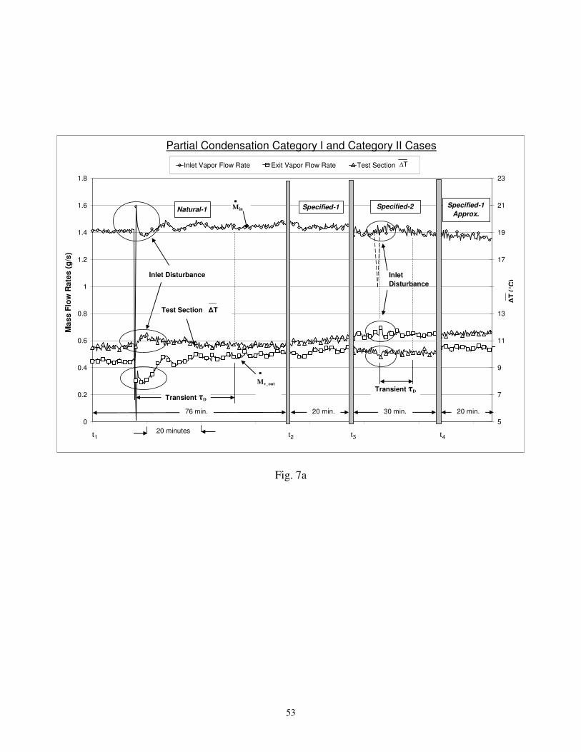
53

0

0.2

0.4

0.6

0.8

1

1.2

1.4

1.6

1.8

5

7

9

11

13

15

17

19

21

23

Inlet Vapor Flow Rate Exit Vapor Flow Rate Test Section

Min

.

t1 t2 t3

76 min. 20 min. 30 min.

∆T

(° C

)

__

Natural-1 Specified-1 Specified-2 Specified-1

Approx.

20 min.

t4

Mv_out

.

Partial Condensation Category I and Category II Cases

20 minutes

Ma

ss F

low

Rate

s (

g/s

)

Inlet Disturbance Inlet

Disturbance

∆T

Transient τD

Transient τD

Test Section ∆T

__

Fig. 7a

54

Test Section (Sub-System B) Pressures

80

84

88

92

96

100

104

108

112

116

120

0 20 40 60 80 100 120 140

Time

Pre

ssu

res:

Pin

let,

Px6

, P

x9 (

kP

a)

-5

-4

-3

-2

-1

0

1

2

3

4

5

Pin Px6 Px9 P

76 min. 20 min. 20 min.30 min.

t1 t2 t3 t4

Natural-1 Specified-1 Specified-2Specified-1

Approx.

20 minutes

. ∆P

( k

PA

)

∆

Inlet Disturbance

Inlet Disturbance

∆P

Inlet Pressure

Exit Pressure

Transient τD

Transient τD

Fig. 7b

55

Test Section (Sub-System B) Temperatures

40

42

44

46

48

50

52

54

56

58

60

0 20 40 60 80 100 120 140

Time

Te

mp

era

ture

s (

°C)

Tx1 Tx4 Tx9 Saturation Temperature

76 min. 20 min. 20 min.30 min.

t1 t2 t3

t4

Natural-1 Specified-1 Specified-2Specified-1

Approx.

20 minutes

.

Inlet Disturbance

Inlet Disturbance

Wall Temperatures

Transient τD

Transient τD

Fig. 7c

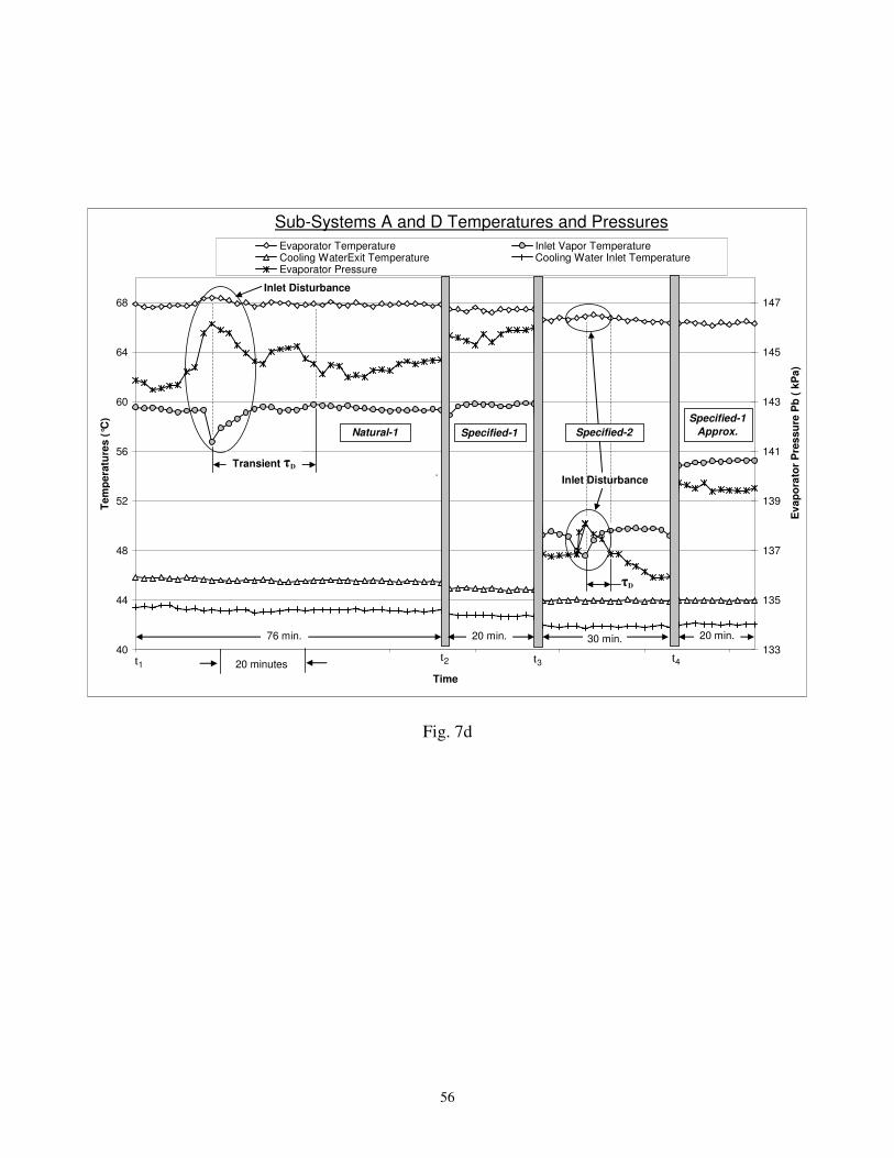
56

40

44

48

52

56

60

64

68

0 20 40 60 80 100 120 140

Time

Te

mp

era

ture

s (

°C)

133

135

137

139

141

143

145

147

Evaporator Temperature Inlet Vapor TemperatureCooling WaterExit Temperature Cooling Water Inlet TemperatureEvaporator Pressure

76 min. 20 min. 20 min.30 min.

t1 t2 t3 t4

Natural-1 Specified-1 Specified-2

Specified-1

Approx.

20 minutes

.

Sub-Systems A and D Temperatures and Pressures

Ev

ap

ora

tor

Pre

ss

ure

Pb

( k

Pa

)

Inlet Disturbance

Inlet Disturbance

Transient τD

τD

Fig. 7d

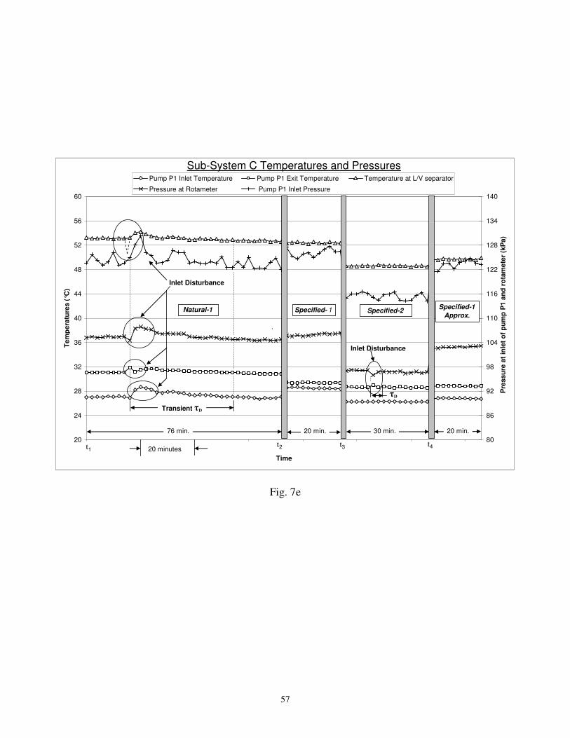
57

20

24

28

32

36

40

44

48

52

56

60

0 20 40 60 80 100 120 140

Time

Te

mp

era

ture

s (

°C)

80

86

92

98

104

110

116

122

128

134

140

Pump P1 Inlet Temperature Pump P1 Exit Temperature Temperature at L/V separator

Pressure at Rotameter Pump P1 Inlet Pressure

76 min. 20 min. 20 min.30 min.

t1 t2 t3 t4

Natural-1 Specified- 1 Specified-2Specified-1

Approx.

20 minutes

.

Sub-System C Temperatures and Pressures

Pre

ss

ure

at

inle

t o

f p

um

p P

1 a

nd

ro

tam

ete

r (k

Pa)

Inlet Disturbance

Inlet Disturbance

Transient τD

τD

Fig. 7e

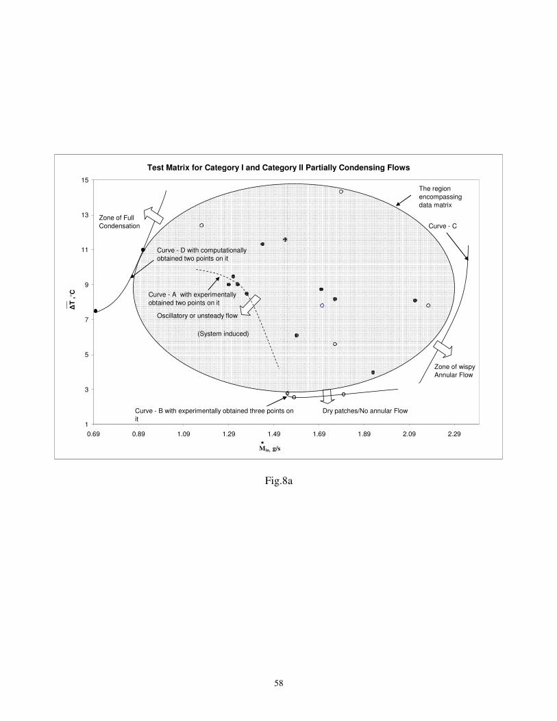
58

Test Matrix for Category I and Category II Partially Condensing Flows

1

3

5

7

9

11

13

15

0.69 0.89 1.09 1.29 1.49 1.69 1.89 2.09 2.29

∆T

,° C

__

Min, g/s.

Curve - B with experimentally obtained three points on

it

Dry patches/No annular Flow

The region

encompassing

data matrix

Curve - C

Zone of Full

Condensation

Zone of wispy

Annular Flow

Curve - A with experimentally

obtained two points on it

Curve - D with computationally

obtained two points on it

Oscillatory or unsteady flow

(System induced)

Fig.8a

59

Fig. 8b

0.00

0.25

2.1

0.50

0.75

1.8151.510

1.25

Category II "Natural Exit" Cases

Category I "Specified Exit" Cases

Representative Oscillatory Flow

Min, g/s

.

∆T ,°C

Ze

-

3-D Test Matrix for Category I and Category II Partially Condensing Flows

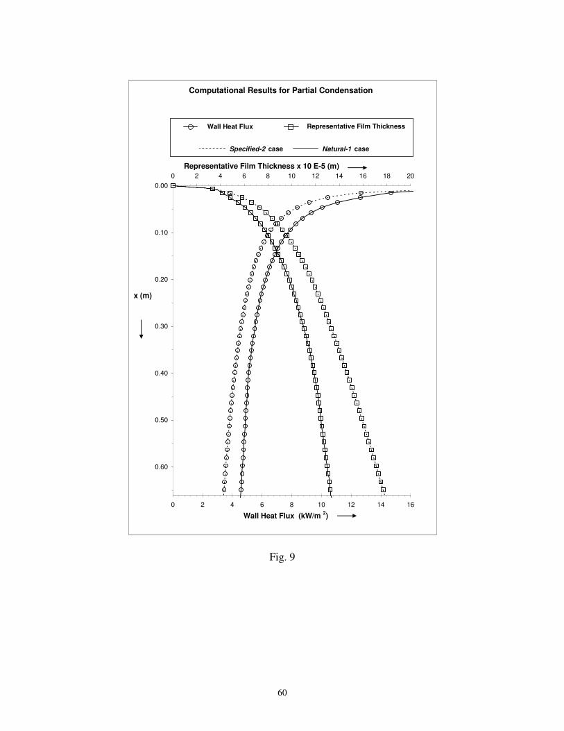
60

Fig. 9

0 2 4 6 8 10 12 14 16 18 20

0.00

0.10

0.20

0.30

0.40

0.50

0.60

x (m)

Representative Film Thickness x 10 E-5 (m)

0 2 4 6 8 10 12 14 16

Computational Results for Partial Condensation

Wall Heat Flux Representative Film Thickness

Wall Heat Flux (kW/m 2)

Specified-2 case Natural-1 case

61

xfc

E(pressure = pe)

FC

(pressure = pfc)

g

Average zero

vapor mass flow,

zero interfacial

mass flow region

insatin

.

p,T,M

L

Fig. 10

62

Test Matrix for Full Condensation Category II flows

0

5

10

15

20

25

30

35

40

45

50

0 0.5 1 1.5 2 2.5

∆T

,° C

__

Min, g/s.

The region of

plug/slug flow

Curve-X with experimentally

obtained two points on it

Data matrix region

containing maximum

data points for Full

Condesation

The region in which Full

Condensation point exists

out of the test section

The region of Full Condesation

inside the test section

Curve-Y

Computationally obtained two

points on boundary Y

Fig. 11

63

Category II Full Condensation Cases

0

5

10

15

20

25

30

35

40

1/0/1900 2/19/1900 4/9/1900 5/29/1900 7/18/1900 9/6/1900 10/26/1900

Time

0

0.2

0.4

0.6

0.8

1

1.2

1.4

1.6

Inle

t V

ap

or

Ra

te (

g/s

)

Test Section Inlet Vapor Rate

Inlet disturbance

Exit disturbance

Test Section ∆T

__

Natural - 1 Natural - 2Natural - 1

Repeated

Min

.

t1 t2 t3

30 min.

3 min.

∆T

__

30 min.30 min.

∆T

Fig. 12a

64

Test Section (Sub-system B) Pressures

40

50

60

70

80

90

100

110

120

130

1/0/1900 2/19/1900 4/9/1900 5/29/1900 7/18/1900 9/6/1900 10/26/1900

Time

Pre

ss

ure

s:

Pin

let , P

x6

, P

(

kP

a)

-5

-4

-3

-2

-1

0

1

2

3

4

DP

(kP

a)

P Px6 P DP∆P

t1 t2 t3

30 min.

3 min.

Natural - 1 Natural - 2Natural - 1

Repeated

∆P

(kP

a)

Inlet disturbance

Exit disturbance

inlet T"

T"

30 min. 30 min.

Fig. 12b

65

Test Section (Sub-system B)Temperatures

20

25

30

35

40

45

50

55

60

65

1/0/1900 2/19/1900 4/9/1900 5/29/1900 7/18/1900 9/6/1900 10/26/1900

Time

Tem

pe

ratu

re,

C

Tx1 Tx4 Tx9 Tsat

Tem

pe

ratu

re (

°C)

t1 t2 t3

30 min.

3 min.

Natural - 1 Natural - 2Natural - 1

Repeated

Exit disturbance

30 min. 30 min.

Inlet disturbance

Fig. 12c

66

Sub-systems A and D Temperatures and Pressures

0

10

20

30

40

50

60

70

80

1/0/1900 2/19/1900 4/9/1900 5/29/1900 7/18/1900 9/6/1900 10/26/1900

Time

Tem

pera

ture

, C

10

30

50

70

90

110

130

150

170

Eva

po

rato

r P

ress

ure

Pb

(k

Pa)

Test Section Inlet Temperature (Tv-in)" Cooling Water Inlet Temperature (Tc1) Evaporator Temperature (Tb)

Cooling Water Exit Temperature (Tc2) Evaporator Pressure Pb

Te

mp

era

ture

(°C

)

t1 t2 t3

30 min.

3 min.

Natural - 1 Natural - 2Natural - 1

Repeated

Exit disturbanceInlet disturbance

30 min. 30 min.

Fig. 12d

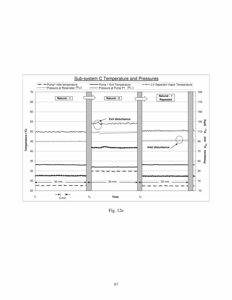
67

Sub-system C Temperature and Pressures

20

25

30

35

40

45

50

55

60

65

70

1/0/1900 2/19/1900 4/9/1900 5/29/1900 7/18/1900 9/6/1900 10/26/1900

Time

Te

mp

era

ture

, C

-10

10

30

50

70

90

110

130

150

170

190

Pre

ss

ure

s

a

nd

(kP

a)

Pump1 Inlet temperature Pump 1 Exit Temperature LV Separator Vapor Temperature

Pressure at Rotameter Pressure at Pump P1

Te

mp

era

ture

,°C

Tem

pe

ratu

re (

°C)

t1 t2 t3

30 min.

3 min.

Natural - 1 Natural - 2Natural - 1

Repeated

Exit disturbance

Inlet disturbance

(PD2) (PP1')

PD

2P

P1

'

30 min. 30 min.

Fig. 12e

68

0

0.2

0.4

0.6

0.8

1

1.2

1.4

1.6

Timet1 t2 t3

Instability at Lower Flow Rate for Category II Full Condensation

Inle

t V

ap

or

Mas

s F

low

Ra

te (

g/s

)

Natural -

1

Natural - 2 Unstable Zone, No steady Solution Exists

15 min. 60 min.

15 min.

15 min.

Fig.13a

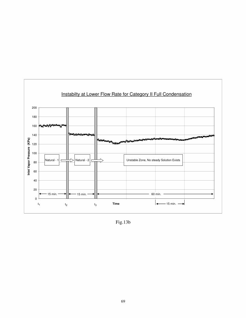
69

0

20

40

60

80

100

120

140

160

180

200

Time

Natural - 1

t1 t2 t3

15 min. 60 min.

Instabilty at Lower Flow Rate for Category II Full Condensation

Inle

t V

ap

or

Pre

ss

ure

(K

Pa)

Natural - 2 Unstable Zone, No steady Solution Exists

15 min.

15 min.

Fig.13b

70

Fig. 14

0 2 4 6 8 10 12 14 16

0.00

0.02

0.04

0.06

0.08

0.10

0.12

0.14

0.16

0.18

0.20

x (m)

Representative Film Thickness x 10 E-5 (m)

0 5 10 15 20 25 30 35 40 45 50

Computational Results for Full Condensation

Wall Heat Flux Representative Film Thickness

Wall Heat Flux (kW/m 2)

xfc=

71

Oscillatory Category II Partial Condensation Flow

0.3

0.5

0.7

0.9

1.1

1.3

1.5

1.7

Time

Ma

ss

Flo

w R

ate

(g

/s)

-3

-2.5

-2

-1.5

-1

-0.5

0

0.5

Inlet Vapor Mass Rate Exit Vapor Mass Rate

Exit Liquid Flow Rate Test Section

30 min.

Min

.

MV

.

3 min.

ML

.

∆P

Min

.MV

.

ML

.

Te

st

Sec

tio

n ∆

P (

kP

a)

∆P

Fig. 15a

72

97

99

101

103

105

107

109

111

Time

Pre

ssu

re (

Kp

a)

46.5

47

47.5

48

48.5

49

49.5

50

Inlet Vapor Pressure Pressure Exit Pressure Temperature at Rotameter

30 min.

px6

(px6)

pin

(pin)

3min.

Oscillatory Category II Partial Condensation Flow

pexit

(pexit)

Tem

pe

ratu

re (

°C)

(TR)

TR

Fig.15b

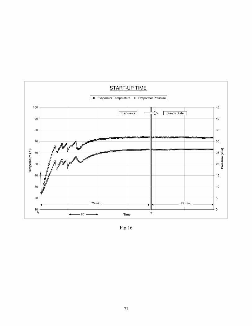
73

START-UP TIME

10

20

30

40

50

60

70

80

90

100

Time

0

5

10

15

20

25

30

35

40

45

Pre

ssu

re (

kP

a)

Evaporator Temperature Evaporator Pressure

Transients

t1

75 min. 45 min.

Tem

pe

ratu

re (

°C)

Steady State

20

mi

t2

Fig.16

74

Table 1

• *The error values for this case were greater than the representative error values shown in the column headers due to small T∆

and high relative error associated with its measurement.

• NA: The data was not available due to some equipment problem

inM& VM&

Ze

exp

Ze

comp wT Tsat T∆ pin px6 pT" ∆p pD2 ρ 2/ρ1 µ2/µ1 G Re Ja Pr1 outQ&

q ′′′′′′′′ h

(g/s) (g/s)

(K) (K) (K) (kPa) (kPa) (kPa) (kPa) (kPa) (kg/m2s) (J/s) (W/m2) (W/m2K)

Run

No.

±0.05 ±0.04 ±0.04

±1 ±0.15 ±1 ±0.6 ±0.6 ±0.7 ±0.05 ±2 ±0.0001 ±0.0001 ±1.5 ±900 ±0.02 ±0.02 ±5 ±800 ±80

1 1.44 0.48 0.33 0.33 320 331.49 11 107.3 109.3 106.5 -0.82 105 0.0085 0.0243 42.1 23900 0.14 9.61 81 5200 453

2 1.76 1.08 0.62 0.57 317 325.23 8 87.0 86.4 88.0 -0.36 85 0.0070 0.0223 51.5 29700 0.10 10.11 58 3700 450

3 1.54 0.69 0.44 0.36 323 335.55 12 122.6 116.6 116.1 -0.19 114 0.0097 0.0260 45.0 25300 0.15 9.21 71 4500 387

4 1.29 0.49 0.38 0.38 320 329.64 10 101.0 102.4 100.8 -2.09 98 0.0081 0.0230 37.7 21500 0.11 9.69 68 4300 476

5 1.70 0.83 0.51 0.52 324 332.55 9 111.0 112.5 111.0 -0.93 109 0.0089 0.0252 49.6 28100 0.11 9.37 70 4400 508

6 1.17 0.47 0.40 0.39 320 332.64 13 111.3 NA 111.3 -0.12 109 0.0088 0.0246 34.2 19325 0.16 9.55 59 3700 298

7 1.31 0.49 0.37 0.37 321 330.85 10 105.0 106.8 104.5 -2.06 102 0.0084 0.0244 38.3 21700 0.12 9.58 69 4400 462

8* 1.93 1.39 0.72 0.72 322 325.55 4 84.6 NA NA 0.01 NA 0.0071 0.0231 56.4 32500 0.05 9.85 47 3000 742

9 1.59 1.11 0.69 0.63 328 334.25 6 113.0 NA NA NA NA 0.0094 0.0265 46.5 26200 0.08 9.07 40 2500 418

10 2.12 1.37 0.64 0.64 320 327.85 8 91.4 NA NA -0.10 NA 0.0076 0.0234 62.0 35500 0.10 9.83 64 4100 503

11 1.30 0.45 0.35 0.38 321 329.29 8 99.8 100.2 99.7 -1.62 97 0.0080 0.0240 38.0 21700 0.10 9.70 72 4600 537

75

Table 2

• *The error values for this case were greater than the representative error values shown in the column headers due to small T∆ and

high relative error associated with its measurement.

• NA: The data was not available due to some equipment problem

inM& V

M&

Ze-

exp wT

Tsat ∆T pin px6 pT" ∆p pD2 ρ 2/ρ1 µ2/µ1 G Re Ja Pr1 outQ&

q ′′ h

(g/s) (g/s)

(K) (K) (K) (kPa) (kPa) (kPa) (kPa) (kPa) (kg/m2s) (J/s) (W/m2) (W/m2K)

Run

No.

±0.05 ±0.04 ±0.04 ±1 ±0.15 ±1 ±0.6 ±0.6 ±0.7 ±0.05 ±2 ±0.0001 ±0.0001 ±1.5 ±900 ±0.02 ±0.02 ±5 ±800 ±80

1 1.44 0.52 0.36 320 331.91 12 108.8 110.9 108.0 -1.82 106 0.0087 0.0244 42.1 23800 0.15 9.59 78 4900 416

2 1.31 0.50 0.38 320 329.16 9 99.4 100.3 99.5 -0.43 98 0.0080 0.0238 38.4 21900 0.11 9.72 69 4400 505

3 1.34 0.59 0.44 320 328.55 9 97.4 98.4 97.3 -0.32 96 0.0078 0.0236 39.1 22400 0.10 9.76 64 4100 491

4* 1.80 0.64 0.36 323 330.53 8 103.9 105.9 104.4 -0.59 103 0.0083 0.0246 52.6 29900 0.09 9.50 97 6200 851

5* 1.92 1.00 0.52 323 329.64 7 101.0 103.3 101.7 -0.40 100 0.0081 0.0244 56.1 32000 0.08 9.55 78 4900 771

6 1.20 0.00 0.00 320 332.23 12 110.5 113.2 110.5 -0.80 108 0.0088 0.0245 35.0 19800 0.16 9.57 101 6400 514

7 1.22 0.44 0.35 320 331.71 12 108.0 110.6 108.0 -0.62 106 0.0086 0.0243 36.6 20200 0.15 9.62 66 4200 351

8* 1.93 1.15 0.60 322 325.21 3 87.15 NA NA -1.30 NA 0.0071 0.0231 56.4 32600 0.04 9.87 67 4300 1174

9 1.61 1.14 0.70 322 332.57 11 111.4 104.6 107.0 -0.87 103 0.0089 0.0250 47.1 26630 0.13 9.46 35 2200 212

10 1.67 1.37 0.82 322 331.45 10 105.8 98.6 100.8 -0.74 97 0.0085 0.0245 49.0 27800 0.12 9.57 16 1000 108

11 1.81 1.02 0.56 317 331.48 14 106.8 102.1 NA -0.58 99 0.0085 0.0237 52.9 30000 0.18 9.80 54 3400 236

12 1.66 0.60 0.36 318 333.15 15 113.5 108.6 NA -1.46 106 0.0090 0.0243 48.5 27400 0.20 9.66 88 5600 363

13 1.71 0.49 0.28 316 331.14 15 108.0 107.9 108.1 -2.10 105 0.0085 0.0237 50.1 28400 0.19 9.81 103 6500 441

14 1.30 0.65 0.50 320 326.34 6 90.5 92.1 90.5 -1.15 88 0.0073 0.0230 38.0 21800 0.08 9.90 56 3500 545

15 1.29 0.55 0.43 321 331.63 11 107.7 113.2 110.1 -1.60 107 0.0086 0.0245 37.7 21400 0.14 9.57 62 3900 366

16 1.31 0.76 0.58 321 331.07 11 105.8 109.1 105.8 -0.95 104 0.0084 0.0243 38.3 21700 0.13 9.62 46 2900 279

17 1.14 0.88 0.77 319 326.73 8 91.6 92.8 91.9 -0.14 90.4 0.0074 0.0230 33.5 19300 0.09 9.92 22 1400 186

18 1.39 0.64 0.46 318 329.01 11 98.9 101.3 98.4 -0.65 97.1 0.0079 0.0234 40.6 23200 0.14 9.85 64 4100 377

76

Table 3

• NA: The data was not available due to some equipment problem

inM& wT Tsat ∆T

pin px6 pT" ∆p pD2 ρ 2/ρ1 µ2/µ1 G Re Ja Pr1 outQ& q ′′ h

(g/s) (K) (K) (K) (kPa) (kPa) (kPa) (kPa) (kPa) (kg/m2s) (J/s) (W/m2) (W/m2

K)

Run

No.

±0.05 ±1 ±0.15 ±1 ±0.6 ±0.6 ±0.7 ±0.05 ±2 ±0.0001 ±0.0001 ±1.5 ±800 ±0.02 ±0.02 ±5 ±500 ±26

1 0.69 304 326.93 23 92.3 94.9 90.8 -1.13 89 0.0073 0.0207 20.2 11600 0.28 10.74 59 3800 165

2 0.70 304 328.46 24 97.2 99.8 95.5 -1.54 94 0.0077 0.0210 20.4 11700 0.30 10.65 60 3800 156

3 1.01 317 329.67 13 101.1 104.0 100.1 -0.57 99 0.0081 0.0234 29.7 17000 0.16 9.87 86 5500 438

4 0.86 316 330.20 14 102.8 104.1 101.4 -3.05 99 0.0082 0.0234 25.1 14300 0.17 9.88 73 4600 331

5 0.96 304 326.95 23 92.4 93.1 90.4 -0.62 89 0.0074 0.0208 28.1 16000 0.28 10.72 82 5200 230

6 0.75 302 328.61 27 97.6 98.2 95.4 -3.01 92 0.0077 0.0207 22.0 12500 0.33 10.79 64 4000 151

7 0.62 302 327.17 25 93.0 94.8 91.1 -2.41 89 0.0074 0.0204 18.1 10400 0.31 10.86 53 3375 133

8 0.63 301 326.97 26 92.4 94.2 90.5 -0.54 90 0.0073 0.0203 18.4 10600 0.39 10.90 54 3400 134

9 0.48 301 327.07 26 92.8 94.6 90.7 -1.18 90 0.0074 0.0209 14.0 8000 0.32 10.90 41 2600 102

10 0.78 305 341.13 36 146.0 NA NA -0.35 129 0.0116 0.0240 22.9 12700 0.47 9.95 64 4100 112

11 0.97 316 343.27 27 155.8 NA NA -0.33 140 0.0127 0.0265 28.3 15600 0.37 9.25 79 5000 180

12 0.87 300 343.11 43 155.0 NA NA -0.14 138 0.0125 0.0236 25.4 14000 0.57 10.06 71 4500 104

13 0.80 306 342.02 36 150.0 NA NA -0.25 136 0.0120 0.0244 23.4 12900 0.48 9.80 65 4200 115

14 0.80 322 340.69 19 144.1 135.7 140.4 -0.29 143 0.0115 0.0277 23.6 13000 0.25 9.04 66 4200 228

15 0.99 324 342.32 18 151.4 NA 152.3 -2.05 148 0.0123 0.0279 29.2 16000 0.24 8.87 81 5200 283

16 1.59 306 333.56 27 115.0 110.5 109.3 -0.24 112 0.0090 0.0225 46.4 26100 0.35 10.25 133 8400 309

17 0.76 324 337.82 14 131.7 125.7 126.3 -0.23 130 0.0105 0.0266 22.2 12400 0.18 9.10 63 4000 289

18 1.30 312 342.32 30 109.4 111.4 108.5 -1.32 107 0.0122 0.0256 38 20900 0.40 9.46 107 6700 223