Intermolecular multiple quantum coherences in liquids

Intermolecular MultipleQuantum Coherencesin LiquidsWOLFGANG RICHTER,1 WARREN S. WARREN2

1National Research Council, Institute for Biodiagnostics, Winnipeg, Manitoba, Canada2 Princeton University, Princeton, New Jersey 08544

ABSTRACT: In the early 1990s, the traditional framework of NMR spectroscopy waschallenged through a series of simple experiments. The pulse sequences used consisted of afew RF pulses and a few gradient pulses, and the samples were mixtures of simplemolecules. The spectra showed unexpected cross peaks between spins in different molecules.

( )In order to explain these results, two basic assumptions had to be revisited: 1 the( )high-temperature approximation to the Boltzmann distribution at equilibrium, and 2 the

cancellation of dipolar couplings in solution. A close look at the physics involved showedthat correlations between spins in separate molecules exist even after a single pulse, andthat dipolar couplings can make these correlations visible in the presence of gradientpulses. A comprehensive description of the effect is given here, and some present and futureapplications are discussed. � 2000 John Wiley & Sons, Inc. Concepts Magn Reson 12: 396�409,

2000

KEY WORDS: high-temperature approximation; multiple quantum coherences; dipolarcouplings; CRAZED; density matrix

1. INTRODUCTION

Ž .Since the first experiments in 1945 1 , NMR hasarguably become the most versatile and broadlyapplicable form of spectroscopy. NMR is beingsuccessfully applied to solid, liquid, and gaseousmedia, to materials and living systems, and in theinvestigation of microscopic and macroscopicstructures.

One reason for the enduring success of NMRis that the underlying physical phenomena are

Received 10 February 2000; revised 1 May 2000;accepted 5 May 2000.

Correspondence to: Dr. Wolfgang Richter

Ž . Ž .Concepts in Magnetic Resonance, Vol. 12 6 396�409 2000� 2000 John Wiley & Sons, Inc.

extremely well understood. This is especially so inthe case of liquid-state high-resolution NMRspectroscopy. Transitions between nuclear spinstates are virtually independent of other energystates of the molecules. Therefore, for example,the approximation of a two level system to a solehydrogen nucleus in some molecule is indeed avery good one. Nobody seriously doubts that theresponse of a spin system to some sequence ofradiofrequency pulses, delays, and gradients canbe predicted with very high accuracy, even forpulse sequences consisting of thousands of RF

Žpulses and delays. The accuracy is not arbitrarilyhigh, however, because some chaotic dynamicsmight occur, due to radiation damping or residual

Ž . .dipolar couplings 2 . If the spectrum that isproduced by such a pulse sequence deviated from

396

INTERMOLECULAR MULTIPLE QUANTUM COHERENCES IN LIQUIDS 397

theoretical predictions, we would immediately as-sume that the spectrometer did not execute thepulse sequence properly.

Thus it was extraordinarily surprising when, inthe early 1990s, a series of experiments was per-

Ž .formed 3�4 , whose results seemed to contradictconventional NMR theory. In these experiments,

Žextremely simple pulse sequences for example,two RF pulses and one or two gradient pulses,such as in the CRAZED sequence or the HO-MOGENIZED sequence, which are discussed be-

.low were applied to sometimes extremely simpleŽspin systems for example, a mixture of benzene

and chloroform; each of these molecules contains.only a single distinguishable proton . A shown in

Figs. 1 and 2, the resulting spectra showed largeŽpeaks no more than an order of magnitude be-

low the peak corresponding to the full magnetiza-.tion at positions where there was no peak ex-

pected. The positions of these peaks correspondto those that would be produced by intermolecu-lar multiple-quantum transitions, which had notbeen observed before in liquids, for a variety ofperceived reasons, which will be discussed in de-tail below.

Several possible theories to explain these extrapeaks were put forward at that time. A hint of thecorrect explanation is actually contained in a

Ž .seemingly unrelated and much older paper 5 ; aŽ .recent article 6 describes this connection very

Ž .nicely. In the experiment described in 5 , a two-pulse sequence is applied to a sample of solidHelium-3 in the presence of a constant magneticfield gradient; a similar experiment was later per-

Figure 1 CRAZED spectrum of a mixture of benzeneand chloroform. By conventional theory, this spectrumshould be blank. Instead, there are peaks with allproperties of intermolecular double-quantum peaks.

Figure 2 HOMOGENIZED spectrum of a mixture ofbenzene and chloroform. By conventional theory, thisspectrum should be blank. Instead, there are peakswith all properties of intermolecular zero-quantumpeaks.

formed, at much higher field, on a sample ofŽ .water 7 . This experiment produced a series of

Ž .echoes in the free induction decay FID . Theseechoes were explained through the concept of the‘‘dipolar demagnetizing field.’’ According to thisexplanation, the magnetic field gradient leads tothe appearance of a dipolar field which makes thedynamics of the spin system nonlinear and there-fore causes harmonics in the FID. This is theorigin of a classical explanation of the extra peaksobserved in 2D experiments. However, a quantummechanical explanation was put forward as well.The classical explanation, while equally correct,lacks the predictive and intuitive power of thequantum mechanical one. For example, it is easyto see from the quantum mechanical picture whya pulse sequence like the HOMOGENIZED se-

Žquence Fig. 2; see a brief discussion of this se-.quence at the end of this article can produce

narrow-line spectra in extremely inhomogeneoussamples. A classical explanation of this is ex-tremely awkward. In this article, therefore, wewill focus on the quantum mechanical explana-tion.

Two assumptions that are explicitly or implic-itly made in all textbooks have to be discarded.One of these assumptions concerns the equilib-rium density operator for the spin system, and theother one concerns the dipolar interactions be-tween spins. It turns out that these conventionalassumptions predict experimental results cor-rectly, as long as there are no gradient pulses inthe pulse sequence. In the presence of gradientpulses, these assumptions have to be revisited, asexplained below. It would also fail for a sample

RICHTER AND WARREN398

whose shape is far from spherical; this has beenŽ .demonstrated experimentally by both Edsez 8

Ž .and Jeener 9 .

2. EARLY UNEXPECTED RESULTS:THE CRAZED EXPERIMENT

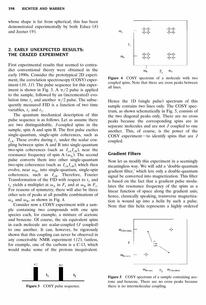
First experimental results that seemed to contra-dict conventional theory were obtained in theearly 1990s. Consider the prototypical 2D experi-

Ž .ment, the correlation spectroscopy COSY exper-Ž .iment 10, 11 . The pulse sequence for this exper-

iment is shown in Fig. 3. A ��2 pulse is appliedŽ .to the sample, followed by an incremented evo-

lution time t and another ��2 pulse. The subse-1quently measured FID is a function of two timevariables, t and t .1 2

The quantum mechanical description of thispulse sequence is as follows. Let as assume thereare two distinguishable, J-coupled spins in thesample, spin A and spin B. The first pulse excitessingle-quantum, single-spin coherences, such asI . These evolve during t under the scalar cou-xA 1pling between spins A and B into single-quantum

Ž .two-spin coherences such as I I , near theyA z BŽ .resonance frequency of spin A � . The secondA

pulse converts them into other single-quantumŽ .two-spin coherences such as I I , which thenzA yB

evolve, near � , into single-quantum, single-spinBcoherences, such as I . Therefore, Fourierx BTransformation of the FID with respect to t and1t yields a multiplet at � in F and at � in F .2 A 1 B 2For reasons of symmetry, there will also be threeother sets of peaks at all possible combinations of� and � , as shown in Fig. 4.A B

Consider now a COSY experiment with a sam-ple containing two compounds with one spinspecies each, for example, a mixture of acetoneand benzene. Of course, the six equivalent spins

Ž .in each molecule are scalar-coupled J coupledto one another. It can, however, be rigorouslyshown that this coupling can never be observed in

Ž . Žany conceivable NMR experiment 12 , unless,for example, one of the carbons is a C-13, whichwould make some of the protons inequivalent.

Figure 3 COSY pulse sequence.

Figure 4 COSY spectrum of a molecule with twocoupled spins. Note that there are cross peaks betweenall lines.

Ž .Hence the 1D single pulse spectrum of thissample contains two lines only. The COSY spec-trum, as shown schematically in Fig. 5, consists ofthe two diagonal peaks only. There are no crosspeaks because the corresponding spins are inseparate molecules and are not J coupled to oneanother. This, of course, is the power of theCOSY experiment�to identify spins that are Jcoupled.

Gradient Filters

Now let us modify this experiment in a seeminglymeaningless way. We will add a ‘double-quantumgradient filter,’ which lets only a double-quantumsignal be converted into magnetization. This filteris based on the fact that a gradient pulse modu-lates the resonance frequency of the spins as alinear function of space along the gradient axis;hence, classically speaking, transverse magnetiza-tion is wound up into a helix by such a pulse.Note that this helix represents a highly ordered

Figure 5 COSY spectrum of a sample containing ace-tone and benzene. There are no cross peaks becausethere is no intermolecular coupling.


state, which has, however, no net magnetizationassociated with it. This helix can subsequently beunwound by another gradient pulse of oppositepolarity. This classical picture can be extended to

Žmultiple-quantum coherences there is no helix ofa measurable quantity then, but the analogy is

.valid . If a gradient pulse is applied to a double-quantum coherence, which naturally evolves at

Ž .twice the basic resonance frequency, the virtualhelix that is created has only half the pitch of thehelix created by the same gradient applied to asingle-quantum coherence. In other words, thedouble-quantum helix is twice as tightly wound upas the single-quantum helix. It follows that a pairof gradient pulses whose areas are at a ratio of1:2 acts as a double-quantum filter�a quantitythat is magnetization after this filter has to havebeen a double-quantum coherence during the firstgradient pulse; then and only then would thesecond gradient pulse exactly unwind the helixand create net magnetization. This also meansthat, if there is magnetization after this filter, a2-quantum to 1-quantum transformation musthave taken place between the two gradient pulses.

We will now add a double-quantum gradientfilter at the second pulse of the COSY experi-ment, as shown in Fig. 6. G is the amplitude ofthe first gradient, and T is its duration; the areaof the second gradient pulse is twice that of thefirst one. It is easy to see that there is no signalexpected after this pulse sequence. As mentionedabove, the first pulse of the COSY experimentcreates single-quantum coherences, which will notpass the double-quantum filter. Hence, accordingto conventional NMR theory and prior to 1990,no one would have expected a signal from thispulse sequence, save for imperfections in thepulses, and effects caused by relaxation. This iswhy this pulse sequence was called the CRAZEDŽCOSY Revamped by Asymmetric Z-Gradient

. Ž .Echo Detection sequence. However, in 2 it wasshown that there is a large signal after this pulsesequence. Peaks appear both on the pseudo-diag-onal F � �2 F , and as cross peaks between1 2

Ž .benzene and acetone protons Fig. 1 .

Figure 6 CRAZED sequence.

What does it mean that there is magnetizationat the end of the gradient filter? It can only be so

Ž .if two conditions are true: 1 There must havebeen a double-quantum coherence evolving be-

Ž .fore the gradient filter; and 2 this coherencemust have been transformed into a single-quan-tum coherence after the first gradient pulse. This,

Ž .in turn, implies two things: 1 A single pulseŽ .must create double-quantum coherences; and 2

there must be a net coupling between benzeneand acetone protons. Both these statements seemto contradict conventional NMR theory, and wewill discuss them now.

3. THE DENSITY OPERATOR

The density operator, commonly designated as �,describes the state of a spin system at any pointduring the pulse sequence. For a comprehensive

Ž .discussion of the density operator, see 13 .At thermal equilibrium, the spin system fol-

lows a Boltzmann distribution. The density opera-tor is given by

Ž .exp �HHHHH��kT� �� 1eq � Ž .�tr exp �HHHHH��kT

Note that we used the Hamiltonian operator, HHHHH,in units of angular frequency. This is often conve-nient in spectroscopic applications; the conven-

Ž .tional Hamiltonian energy operator can be ob-tained by multiplying by �.

Let us discuss some examples. The simplest1one is given by an isolated spin , such as hydro-2

gen, which possesses two energy levels in a mag-netic field. The Hamiltonian of this system isgiven by

� �HHHHH � � I 2z

where I is the unitless angular momentum oper-zator, which here represents the action of thestatic magnetic field, and � is the Larmor fre-quency. A convenient basis set is given by the two

� :basis function � � 1�2, 1�2 and � �� :1�2, �1�2 . The matrix elements of I can bezcomputed by

² � � : ² � � : 1� I � � I �z z �1 0I � �z ž /² � � : ² � � : 0 �1ž /� I � � I � 2z z

� �3


At thermal equilibrium we have for this spin,

Ž . ŽŽ . .exp �HHHHH�kT exp ��kT Iz� � �0 � Ž .� � ŽŽ . .�tr exp �HHHHH�kT tr exp ��kT Iz

��exp � 0ž /2kT

��0 exp �� 0ž /2kT

� Ž Ž .. Ž Ž ..exp � ��2kT � exp � ��2kT� �4

The equilibrium population of the two states isgiven by the diagonal elements of this matrix.Therefore, the ratio of the population of the twostates is

Ž .P exp ��2kT �� exp � 5ž /Ž .P exp ��2kT kT�

An explicit calculation for a 600 MHz machineŽ 9 �1.� � 600 MHz*2� � 3.769*10 s and roomtemperature yields P �P � 1.0001.� �

Now suppose we have two isolated spins in thesystem. Accordingly, there are four energy levels,� � , � � , � � , and � � , and the density1 2 1 2 1 2 1 2operator describing this spin system is repre-sented by a four by four matrix,

� � �² � � :� � I � �1 2 z1 1 2

� � �² � � :� � I � �1 2 z1 1 2I �z1� � � �� 0� � � �

�1 0 0 01 0 �1 0 0 � �� 6

0 0 1 02 � 00 0 0 1

�1 0 0 01 0 �1 0 0I � I �z1 z 2 0 0 �1 02 � 0

0 0 0 �1

�1 0 0 01 0 �1 0 0�

0 0 �1 02 � 00 0 0 �1

�1 0 0 00 0 0 0 � �� 70 0 0 0� 00 0 0 �1

The population ratio between lowest and high-est energy states is therefore

2�� P �P � exp � 1.0002 8�� ž /kT

Similarly, we can calculate the populations for alarge number of spins. For example, for a system

4 Žcontaining 10 spins which would, incidentally,.still be a microscopic sample , we find, for the

ratio of the population of the lowest energy stateand of the highest energy state,

104�� P �P � exp � 2.6 9� � � � ž /kT

Compare these results to the traditional ‘high-temperature’ approximation to the equilibriumdensity operator. In that approximation, the expo-nential is expanded in a truncated Taylor series,as follows:

ŽŽ . .exp ��kT Ý Ii z iHT� �0 � Ž .�tr exp �HHHHH�kT

Ž .1 � ��kT Ý Ii z i � �� 10� Ž .�tr exp �HHHHH�kT

This is very convenient, because we can startany pulse sequence calculation with an equilib-rium state of

� �� I 11eq z i

because I is the only variable that evolves inztime. What are we missing by this approximation?The argument that is commonly given for thevalidity of the approximation is that the Boltz-

Ž �4 .mann factor is a small number ��kT � 10 ,and higher order terms in this expansion aretherefore negligible.

This is a fallacy. If the Taylor expansion werenot truncated, it would continue as

ŽŽ . .exp ��kT Ý Ii z i� �0 � Ž .�tr exp �HHHHH�kT

Ž .1 � ��kT Ý Ii z i2Ž .� ��kT Ý Ý I I � � i j z i z j � �� 12� ŽŽ ..�tr exp �HHHHH�kT

and, even though the quadratic term has a coef-ficient that is several orders of magnitude smaller


than that of the linear term, the double sum inthe quadratic term has N times as many mem-bers as the single sum in the linear term. For atypical NMR sample, N � 1020 and N 2 � 1040 ;hence it is not at all obvious that this expansioneven converges!

Let us now calculate the populations of thestates that are predicted by the high-temperatureapproximation. For a two-spin system, for exam-ple, we find that

��Ž .1 � I � Iz1 z 2kT

��1 � 0 0 0

kT0 1 0 0 � �� 130 0 1 0

�� 00 0 0 1 �kT

which means that the predicted ratio of popula-tions of the highest and lowest energy levels is

Ž .1 � ��kT� �P �P � � 1.0002 14�� Ž .1 � ��kT

in accordance with the exact calculation. How-ever, for 104 spins, we find

Ž .1 � 5000 ��kT� �P �P � � 2.9 15� � � � Ž .1 � 5000 ��kT

which is significantly different from the exactŽ � �.result of 2.6 obtained above Eq. 9 . For larger

number of spins, the two results diverge evenmore. The reason for this is, of course, that theapproximation made by the truncated Taylor se-

Ž .ries, exp x � 1 � x, only holds if x is smallcompared to 1. Hence the high-temperature ap-proximation fails to predict the population of theenergy levels appropriately for any macroscopicsample.

It is possible to express the exact density oper-ator in closed form as a product of individual spin

Ž .operators 14 . However, for the purpose of thisarticle, we will keep the usual expansion andterminate it after the quadratic term. This affordsthe necessary insight into the CRAZED experi-

ment; a generalization to other orders of coher-ence is conceptually straightforward and may be

Ž .found in the primary literature 14 .

4. DIPOLAR COUPLINGS

The classical dipolar interaction energy betweentwo magnetic dipoles 1 and 2 is given by

Ž .Ž .� 1 � r � r0 1 12 2 12E � � � � 3dip 1 23 24� � � � �r r12 12

� �16

where the � are the magnetic moments, and ri i jis the vector connecting them.

The dipolar Hamiltonian is constructed in fullanalogy to this, replacing the classical magneticmoment by its quantum mechanical analogueŽ .15 :

� � �0 k lHHHHH � Ýd 34� rk lk�l

Ž .Ž .I r I rk k l l k l � �� I I � 3 17k l 2ž /rk l

Here, the � are the gyromagnetic ratios of theirespective nuclei. The Hamiltonian operator is,again, given in frequency units. This can berewritten in polar coordinates; we can take alsotake into account that nonsecular terms vanish

Ž .because of the Zeeman interaction 10 . Theremaining dipolar Hamiltonian is

N N � � �0 k lsecH � Ý Ýd 34� 4 rk lk�0 l�0

Ž 2 .Ž .� 1 � 3 cos � 3I I � I Ik l k z l z k l

N N

Ž . � �� D 3I I � I I 18Ý Ý k l k z l z k lk�0 l�0

� � �0 k l 2Ž . � �D � 1 � 3 cos � 19k l k l34� 4 rk l

In this equation, is the angle between thek linternuclear vector and the main magnetic field.We have also defined the ‘dipolar coupling con-stant,’ D . Note that the double sum is unre-k l


stricted; hence each spin pair is counted twice.This is included in the definition of D .k l

What is the magnitude of the dipolar cou-plings? For convenience, we will first calculate the

Žvalue of the dipolar coupling constant for two.protons ,

� � �0 k l 2Ž .D � 1 � 3 cos �k l k l34� 4 rk l

rad 1 � 3 cos2�k l � �� 188.7 � 203ž /s Ž .r �nmk l

˚ Ž .For example, for a distance of 5 A 0.5 nm , and � 90�, we find D � 3020 rad s�1, or approxi-k lmately 480 Hz!

The question arises then why we see sharpŽ .lines less than 1 Hz in a well-shimmed sample at

all in the NMR spectrum of a liquid. If thedipolar couplings are on the order of hundreds ofHz or more for nearby protons, then the spectrallines should be just that wide, and we would notsee any structure in the spectrum. This is, ofcourse, precisely the case for a solid.

There are indeed two separate mechanismsthat produce narrow lines in liquids. One mecha-nism applies to pairs of nearby spins, and oneapplies to spins far apart. Note that, over thesurface of an isotropic sphere, the dipolar interac-tions average to zero because

� 2 � 2�Ž . � � �3 cos � � 1 sin �d �d � � 0 21H H��0 ��0

ŽThe extra factor of sin comes from the fact thatthe number of surface elements on a sphere is

.proportional to sin .The two mechanisms that average out dipolar

couplings are the following.Ž .1 Short range dipolar interactions aerage to

zero through diffusion. For a back-of-the-envelopecalculation, let us assume that the diffusion co-efficient of the liquid is D � 2.3 � 10�9 m2�sŽthis is the diffusion coefficient of water at room

.temperature . The root mean square distance thata molecule diffuses in a given time t in somedirection is

' � �r � 2 Dt 22rms

The effects of individual couplings can be ignoredif they only remain unaltered for a time such that

D t � 1k l

2 2 � �23rad 1 � 3 cos � rk l rmsD t � 188.7 � �k l 3ž /s 2 DŽ .r �nmk l

For our estimation, let us assume that the fullrange of angles is sampled when the spin movesthrough a distance of the order of the intermolec-ular separation. Then, for two spins at the closestpossible distance, say 0.2 nm, we find

2�9Ž .rad 3 0.2�10D t � 188.7 � �k l 3ž /s 2 D0.2

�7 � �� 6.2�10 24

This is indeed much smaller than 1. If we movethe spins farther apart, that number decreaseseven further, as it is approximately inversely pro-portional to the separation distance. This meansthat all indiidual spin�spin dipolar interactionscan be ignored.

Ž .2 Long-range dipolar interactions are aeragedout by magnetic isotropy. For long range dipolarinteractions, the averaging has to be consideredsomewhat differently. Here we have to look at alarge number of virtually constant interactions

Žsimultaneously each individual spin pair does notsample the full range of angles any more, but isvirtually static on an NMR time scale. We willhave to add up all individual interactions, with aproper weighting for each spin pair. If the liquid

Žis magnetically isotropic that is, if the magnetiza-.tion is the same anywhere in the sample , dipolar

interactions add up to zero by virtue of sphericalsymmetry. It is a fallacy to conclude that longrange dipolar interactions are negligible becauseof the r�3 dependence, because the number ofspins at a given distance increases as r 2. The sumof all dipolar interactions at a given spin only fallsoff as r�1.

Therefore, we will have to explicitly considerlong-range dipolar interactions whenever themagnetization of the sample is a function of loca-tion. This happens whenever gradient pulses areapplied during the pulse sequence. Dipolar inter-actions will also reappear whenever the sample isnot spherical. However, in the absence of gradi-ents, the effects of these couplings are usually


masked by radiation damping and will not beconsidered here.

5. QUANTITATIVE ANALYSIS OF THECRAZED EXPERIMENT

5.1. Overview

Considering the discussion of Sections 3 and 4,we can see now how the strange peaks in theCRAZED spectrum originate. The pulse se-quence was given in Fig. 6. The quadratic term inthe equilibrium density operator contains two-spinterms such as I I . A ��2 pulse transforms thisz1 z 2into I I , which is actually a mixture of double-x1 x 2and zero-quantum coherences. Hence double-quantum coherences evolve during t ; they even-1tually give rise to the cross peaks. They also passthe double-quantum gradient filter, because thesecond ��2 pulse transforms a term such asI I into I I , which is a single-quantum,x1 y2 z1 y2two-spin term. By then, the sample exhibits

Žanisotropic magnetization because of the gradi-.ent pulses , and dipolar couplings reappear.

Therefore, dipolar couplings between spins 1 and2 transform �I I into I , which is magnetiza-z1 y2 x 2tion. In Fig. 7, this is depicted schematically.

5.2. Quantitative Analysis

We start out the density matrix calculation withthe expansion terminated after the quadratic term,

2N N N�� 1 �� 1 � I � I I 25Ý Ý Ýz i z i z jž /kT 2 kTi�1 i�1 j�1

We can immediately simplify this, consideringthat only the second order term will survive the

Figure 7 Evolution of some relevant spin operatorsduring the CRAZED sequence.

Ždouble-quantum filter we already know that thehigh-temperature density matrix cannot con-tribute to the signal of the CRAZED sequence,

.as discussed in Sect. 2 . Furthermore, we willleave out all normalizing constants; at the end, wewill compare the signal to that after a singlepulse, which contains the same constants. There-fore we will start with

2 N N1 �� I I 26Ý Ý z i z jž /2 kT i�1 j�1

Now we apply the first pulse. This transforms thedensity operator into

2 N N1 �� I I 27Ý Ý x i x jž /2 kT i�1 j�1

This term now contains a mixture of zero-quan-tum operators and double-quantum operators.

Ž .During the first time interval t , then the system1evolves into

2 N N1 ��Ž . Ž .� � I cos � t � I sin � tÝ Ý x i 1 y i 1ž /2 kT i�1 j�1

Ž . Ž . � �� I cos � t � I sin � t 28x j 1 y j 1

The gradient pulse adds a space-dependentevolution frequency of magnitude �Gs to theinormal evolution frequency of ��, where s isithe location of spin i along the gradient axis. Asdiscussed above, net dipolar couplings are rein-troduced with the first gradient pulse; for simplic-ity, however, we will begin to consider dipolarcouplings only at the end of the second gradientpulse. This is appropriate because the gradient

Žpulses are short in the common implementations.they are on the order of a few milliseconds . The

Ždensity operator at the end of t after the gradi-1.ent is therefore

21 �� ž /2 kT

N N

Ž .� I cos � t � �GTsÝ Ý x i 1 ii�1 j�1

Ž .�I sin � t � �GTsyi 1 i

Ž .� I cos � t � �GTsx j 1 j

Ž . � ��I sin � t � �GTs 29y j 1 j


The second 90� pulse then transforms the densityoperator into

21 �� ž /2 kT

N N

Ž .� �I cos � t � �GTsÝ Ý z i 1 ii�1 j�1

Ž .�I sin � t � �GTsyi 1 i

Ž .� �I cos � t � �GTsz j 1 j

Ž . � ��I sin � t � �GTs 30y j 1 j

Now we can simplify this equation. Rememberthat no more RF pulses follow, and that only RFpulses can change the number of quanta in an

Žoperator the dipolar couplings only contain.zero-quantum operators . Therefore, we only have

to consider single-quantum terms, that is, termswith a single transverse operator from now on.Those terms are,

2 N N��Ž .� � �I cos � t � �GTsÝ Ý z i 1 iž /kT i�1 j�1

Ž . � ��I sin � t � �GTs 31y j 1 j

1The factor of was deleted, because we under-2� �counted the terms in Eq. 31 by a factor of 2.

During the second gradient pulse, this evolvesinto

2 N N��Ž .� � � I cos � t � �GTsÝ Ý z i 1 iž /kT i�1 j�1

Ž . Ž .� I sin � t � �GTs cos 2�GTsy j 1 j j

Ž . Ž . � ��I sin � t � �GTs sin 2�GTs 32x j 1 j j

Note that we have, for convenience, disregardedthe chemical shift evolution during the secondgradient pulse.

We can transform the products of the trigono-metric functions into sums, using the usualtrigonometric identities. We use

cos A sin B cos C1 � Ž . Ž .� sin A � B � C � sin A � B � C4

Ž . Ž .��sin A � B � C � sin A � B � C

� �cos A sin B sin C 331 � Ž . Ž .� cos A � B � C � cos A � B � C4

Ž . Ž .��cos A � B � C � cos A � B � C

Now consider the following simplification:A function that depends on the absolute posi-

tion of the spin in the sample will average to zero.Ž .For example, if a term depends on sin �GTs ,i

then it will average to zero if the gradient pulsewinds up a helix with many turns over the sample.The only terms that do not average to zero in thismanner are the ones that depend solely on a

Ždifference in position, which are the terms sin A. Ž .� B � C and cos A � B � C in the above

equation. Hence we obtain

21 �� ž /4 kT

N N

Ž .� �I I cos 2� t � �GT s � s�Ý Ý z i y j 1 i ji�1 j�1

Ž . � ��I I sin 2� t � �GT s � s 344z i x j 1 i j

We can further simplify this expression by using

Ž .cos A � B � cos A cos B � sin A sin B � �35Ž .sin A � B � sin A cos B � cos A sin B

Note that for every spin pair ‘ij,’ there is anotherinteraction ‘ ji’ in the sample. Since the sine is anodd function, the terms containing sin B in theabove equation vanish. Hence we are left with

21 �� ž /4 kT

N N

Ž .� �I I cos 2� t�Ý Ý z i y j 1i�1 j�1

Ž .�cos �GT s � si j

Ž . Ž .�I I sin 2� t cos �GT s � s 4z i x j 1 i j

21 �� ž /4 kT

N N

Ž .� I I cos 2� t�Ý Ý z i x j 1i�1 j�1

Ž .�I I sin 2� tz i y j 1

Ž . � ��cos �GT s � s 364i j


Now we let this evolve during t , finally using2dipolar couplings. It can be shown that the onlypart of the dipolar Hamiltonian that matters here

Ž .is the longitudinal part 11 . Evolution under thisHamiltonian takes place, for example, as

D I I t12 z1 z 2 �

2 I I 2 I Iz1 x 2 z1 x 2

Ž . Ž . � �� cos D t � I sin D t 37i j y2 i j

In our case, we find

2ÝÝ 3 D I I t 3 ��i j zi z j 2 �Ž .36 ž /8 kT

N N

Ž .� I cos 2� tÝ Ý y j 1i�1 j�1

Ž .�I sin 2� tx j 1

Ž . Ž .� cos �GT s � s sin D ti j i j 2

2 N3 ��Ž .� I cos 2� tÝ y j 1½ž /8 kT j�1

Ž .�I sin 2� tx j 1

N

Ž . Ž .�cos �GT s � s sin D tÝi j i j 2 5i�1

� �38

Finally, we can quantify the term involving thedipolar couplings. Since we are free to choose theorigin of our coordinate system, we can set s � 0iand find

N

Ž .D cos �GTsÝ i j jj�1

� ��2 N 3 cos2� � 10� H 316� V rV

Ž . 2 � �� cos �GTs r sin � dr d� d� 39

The approximation of the sum by an integral isvalid if the distribution of spins can be consideredcontinuous. The integral has a singularity at r � 0,but in reality two spins will have a finite separa-tion. If the volume of the sample is large enough,

the integral converges as

� �23 cos � � 12�H H H 3rr�r ��0 ��0min

2Ž .�cos �GTs r sin � dr d� d�

� �8� 40� � � s3

2� Ž . �3 s z � 1� �s 2

The minimum separation distance r that isminintroduced as the lower limit of the integral is ofcourse mathematically necessary to avoid the sin-gularity at that point, but also physically reason-able, as two spins cannot be separated by a dis-tance of 0. The integral gives us the total effect ofdipolar couplings on a spin at the center of aninfinitely large sample. However, the effect isobviously distance dependent; therefore, let usonly look at the polar part of this integral,

�23 cos � � 12� 2Ž .cos �GTs r sin � d� d�H H 3r��0 ��0

�23 cos � � 1

� 2� � �GTH�GTr��0

Ž . � �� cos �GTr cos � sin � d� 41

This may be numerically solved as a function ofŽ�GTr which is the interspin distance in units of

.gradient helix pitch . It then turns out that thebulk of dipolar interactions that become visiblecomes from pairs of spins by approximately one

Ž .half helix pitch r��GT � � .� � � �Following Eq. 40 , the sum from Eq. 39 be-

comes

N 2N ��0 � �D � � 42Ý i j sV 6j�1

It is now convenient to introduce a new variable,which we will call the ‘dipolar demagnetizing time,’� . With the definition ofd

1� �� 43d �M0 0


and considering that

N�� M � � 440 ž /4V kT

we find that

23 �� ž /8 kT

N

Ž . Ž .� I sin 2�� t � I cos 2�� tÝ x i 1 y i 1i�1

2 �t � kT2 s� �ž /3 � ��d

N1 ��Ž . Ž .� I sin 2�� t � I cos 2�� tÝ x i 1 y i 14 kT i�1

�t �2 s � �� 45ž /�d

Finally, the system evolves under the chemicalŽ .shift as a function of �� t only. This signal2

behaves like a single-quantum transition in t ,2and like a double-quantum transition in t , in1agreement with our experimental results! Inter-estingly, the signal increases during the acquisi-tion time, unlike a regular FID, which decaysduring t . This reflects the action of the dipolar2couplings, which transform two-spin one-quantumoperators into magnetization during t . Of course,2we have not taken relaxation into account, whichcompetes with the action of the dipolar couplingsand eventually leads to signal decay.

What is the magnitude of the signal? Theanalogous signal from a COSY sequence, usingonly the linear term of the density operatorŽ � �.Eq. 12 , is proportional to the Boltzmann factoronly. Therefore, the ratio between the signal in-tensities is given by

S 1 t �CRAZED 2 s � �� 46S 4 �COSY d

Let us quantify this result. The dipolar demagne-� �tizing time, � , was defined previously in Eq. 43 .d

M , the equilibrium magnetization, is of course a0function of the magnetic field strength, and so isthe dipolar demagnetizing time. For a sample of

water, the equilibrium magnetization is given by

1 N B02Ž .M � ��0 4 V kT

1 2 � 6 � 1023

� �6 34 18 � 10 m21

8 �34� 2.68 � 10 � 1.05 � 10 Jsž /sT

14.1T� �23 �11.38 � 10 JK � 298 K

J 1� 0.045 3T m

Therefore, the dipolar demagnetizing time in thatcase is

1 A2sT � Tm3

� �d �7 84� � 10 J � 2.68 � 10 � 0.045J

� 0.066s

This value is for a sample of pure water at 600MHz. As we can see from the definition of � ,dthis quantity is inversely proportional to both thefield strength and the proton concentration inthe sample.

Note that the derivation that we show in thispaper is incomplete, because we terminate theexpansion of the density operator after thequadratic term. Higher order terms in this expan-sion can become visible as well; for example,four-spin, single-quantum operators become mag-netization after three successive dipolar cou-plings. The magnitude of the higher order term isnot negligible. A complete derivation, as shown inŽ .9 , reveals that the FID really increases as y �Ž .J x �x, where x is t �� , and J is the second2 2 d 2

order Bessel function. This function is graphed inFig. 8. Note that the signal initially increases al-most linearly with t �this is the limit in which2the derivation in this paper is valid. Note that themaximum occurs when x � 2.2. For a z gradient,� s � 1, hence the maximum is at approximately130 ms in our example.

Now let us consider the effects of relaxation.Transverse magnetization decays with a time con-

� Žstant T the ‘‘apparent transverse relaxation2.time’’ , which may be as long as 1 s in a well-

shimmed sample, but may also be as short as afew tens of milliseconds, especially in io. This


Figure 8 Theoretical shape of the CRAZED FID inthe absence of relaxation.

limits the practicality of the iDQC method atlower field, where � is long.d

5.3. Classical Description of theCRAZED Experiment

As mentioned above, a parallel description of theCRAZED experiment is purely classical; that is,it only considers the evolution of magnetizationunder the action of RF pulses, the static magneticfield, and dipolar interactions from other spins.Classical description of the CRAZED sequencecan be outlined as follows. During the t , the1spins precess about the static magnetic field ac-cording to the conventional Bloch equations. Thismeans, conceptually, that nothing but magnetiza-

Žtion i.e., nothing that could correspond to dou-.ble-quantum coherences evolves during that time.

When gradient pulses are applied, dipolar cou-plings appear and lead to a nonlinear evolutionŽi.e., the evolution of the spins is dependent on

.the instantaneous state of the spin system . Quan-titative analysis shows that the signal is exactlythe same as the quantum treatment predicts;however, the apparent evolution at twice the res-onance frequency during t is merely an effect of1the nonlinear evolution during the gradient pulsesand t . This description is obviously conceptually2different from the quantum description; a discus-sion of the truth of either of these descriptions isbeyond the scope of this paper. However, as men-tioned above, the predictive power of the quan-tum picture is extremely important for the designof novel pulse sequences using this effect.

6. FIRST APPLICATIONS:HOMOGENIZED AND FMRI

In the past few years, some applications of theCRAZED experiment have begun to emerge. Ingeneral, we are not restricted to intermoleculardouble-quantum coherences, as in the CRAZEDexperiment itself, but, in principle, any order ofintermolecular multiple-quantum coherences maybe achieved through the proper pulse sequence.Hence the general method is called ‘intermolecu-

Ž .lar multiple-quantum coherence iMQC method.’The strength of the iMQC method is that

interactions and relationships between spins canbe measured on a mesoscopic distance scale. Asdiscussed above, the typical interaction distancethat later becomes visible is on the order of 1�2pitch of the gradient helix, which can in practicebe as short as 10 m. This lower limit is approxi-mate and essentially limited by the diffusionproperties of the sample in relation to the lengthof the pulse sequence�if the helix pitch is toshort, diffusion blurs the gradient helix so that itcannot refocus properly.

Most applications to date are based on inter-Ž .molecular zero-quantum coherences iZQCs .

Since the coherence order is generally deter-mined by the ratio of areas of the two gradientpulses, we need only a single gradient pulse toselect for iZQCs. The crucial property of a zero-quantum coherence is that it evolves at the dif-ference of the resonance frequency of the twospins. This means that the linewidth of an iZQCpeak is a function not of the overall distribution

Žof magnetic susceptibilities in the sample the.‘overall inhomogeneity’ , but rather of the distri-

bution of magnetic susceptibility gradients overthe distance scale selected. Consider, for exam-

Ž .ple, the HOMOGENIZED pulse sequence 16 .This pulse sequence is identical to the CRAZED

Ž .sequence, with three modifications: 1 The firstgradient pulse is eliminated, for zero-quantum

Ž .coherence selection; 2 the second RF pulse is a45� pulse�this achieves maximum signal, as a

Ž .simple density operator calculation shows; and 3at the end of the pulse sequence, a spin echo isadded, in order to combat effects of relaxation.

The HOMOGENIZED pulse sequence thendetects magnetization in F , and iZQCs in F .2 1Consequently, when this pulse sequence is ap-plied to a sample in an extremely inhomogeneous

Ž .field, sharp lines can be achieved in F . In 16 , it1was shown that, in spite of a directly detected


linewidth of several hundred Hz, a triplet couldbe resolved in the indirectly detected dimension.

IMQC contrast may also prove invaluable inŽ .magnetic resonance imaging MRI . Since it has

Ž .been shown 17 that the contrast is fundamen-tally different from T , T , or T� , and since there1 2 2are good reasons to believe this contrast corre-lates with oxygenation, it may be very useful indiagnostic imaging. Another exciting applicationin this context is that to functional magnetic

Ž . Ž .resonance imaging fMRI 18�21 . In short,fMRI measures brain function through the relax-ation properties of water protons in the brain.Upon neuronal activation, oxydative metabolismat the site of activation increases. Within a fewseconds, blood flow increases as well and actuallyovercompensates for the increased oxygen de-mand. Hence oxygen concentration in the vicinityof the activated site increases. As a consequence,

Ž .the relative concentration of paramagnetic de-oxyhemoglobin decreases, and the apparenttransverse relaxation time T� increases. There-2fore, an image with T� weighted contrast shows2increased intensity upon neuronal activation. This

Žis called the BOLD ‘blood oxygen level depen-.dent’ effect.

Since functional MRI measures susceptibilitygradients related to brain activation, an iMQCmethod may have vastly improved sensitivity overthe BOLD experiment. The signal change in theBOLD experiment is on the order of a few percent. Considering the already staggering difficul-ties in taking images of a living organism in quicksuccession, it is obvious that we can only detectbrain activation in the most fortunate circum-stances. In the iMQC method, we have severalvariable parameters, most notably, the interaction

Ždistance between the two spins which is thedistance over which susceptibility gradients are

.measured . Even though the BOLD mechanism isnot well understood at present, it is likely that thesusceptibility gradients that change upon activa-tion have a typical length, related to the vesselsize. Therefore it is well possible that an iMQCexperiment with appropriate parameters mightdetect a much larger signal change upon activa-tion. In fact, it has recently been shown by our

Ž .group 22 that functional activation in the visualcortex can be detected by the iMQC method; inthis first experiment, we found that the iMQCactivation map was much more focal than, andnot fully congruent with, the BOLD activationmap. Furthermore, the typical relative signalchange upon activation was several times higher

for the iMQC method. Future work will reveal ifthe iMQC method can indeed be routinely usedfor functional MRI.

7. CONCLUSION

The iMQC method was developed during the pastdecade from observations that seemed to contra-dict the very foundations of NMR. We know nowthat the signal is generated through a mechanismdifferent than that in all other liquid state NMRexperiments. This leads us to believe that aplethora of potential applications of this methodexists; we have given here a glimpse into the twomost exciting applications to date.

REFERENCES

1. Bloch F, Hansen WW, Packard ME. Nuclear in-duction. Phys Rev 1946; 69:127.

Ž2. Lin Y-Y, Lisitza N, Ahn S, Warren WS. Science in.press .

3. He Q, Richter W, Vathyam S, Warren WS. Inter-molecular multiple-quantum coherences and crosscorrelations in solution nuclear magnetic reso-nance. J Chem Phys 1993; 98:6779; Warren WS,Richter W, Hamilton Andreotti A, Farmer III BT.Generation of impossible cross peaks between bulkwater and biomolecules in solution NMR. Science1993; 262:2005.

4. Richter W, Lee S, Warren WS, He Q. Imaging withintermolecular multiple-quantum coherences in so-lution NMR. Science 1995; 267:654�657.

5. Deville G, Bernier M, Delrieux JM. Phys Rev B1979; 19:5666.

6. Minot ED, Callaghan PT, Kaplan N. J Magn Reson1999; 140:200�205.

7. Bowtell R, Bowley RM, Glover P. J Magn Reson1990; 88:643�651.

8. Edzes HT. J Magn Reson 1990; 86:293�303.9. Jeener J, Vlassenbroek A, Broekaert P. J Chem

Phys 1995; 103:1309�1332.10. Jeener J. NMR excitation with two pulses. Ampere

International Summer School. Yugoslavia: BaskoPolje; 1972.

11. Aue W, Bartholdi E, Ernst RR. Two-dimensionalspectroscopy. Application to nuclear magnetic res-onance. J Chem Phys 1976; 64:2229�2246.

12. Abragam A. The principles of nuclear magnetism.Oxford: Clarendon; 1961.

13. Ernst RR, Bodenhausen G, Wokaun A, Principlesof nuclear magnetic resonance in one and twodimensions. Oxford: Clarendon; 1987.


14. Lee S, Richter W, Vathyam S, Warren WS. Quan-tum treatment of the effects of dipole-dipole inter-actions in liquid nuclear magnetic resonance. JChem Phys 1995; 105:874�900.

15. Harris RK. Nuclear magnetic resonance spec-troscopy. London: Pitman; 1983.

16. Bandettini PA, Wong EC, Hinks RS, Tikofsky RS,Hyde JS. Time course EPI of human brain functionduring task activation. Magn Reson Med 1992;25:390�397.

17. Warren WS, Ahn S, Mescher M, Garwood M,Ugurbil K, Richter W, Rizi RR, Hopkins J, LeighJS. MR imaging contrast enhancement based onintermolecular zero quantum coherences. Science1998; 281:247�251.

18. Vathyam S, Lee S, Warren WS. HomogeneousNMR spectra in inhomogeneous fields. Science1996; 272:92�96.

19. Ogawa S, Menon RS, Kim S-G, Ugurbil K. On thecharacteristics of functional magnetic resonanceimaging of the brain. Annu Rev Biophys BiomolStruct 1998; 27:447�474.

20. Kwong KK, Belliveau JW, Chesler DA, GoldbergIE, Weisskoff RM, Poncelet BP, Kennedy DN,Hoppel BE, Cohen MS, Turner R, Cheng H, BradyTJ, Rosen BR. Dynamic magnetic resonance imag-ing of human brain activity during primary sensorystimulation. Proc Natl Acad Sci USA 1992;89:5675�5679.

21. Ogawa S, Tank DW, Menon R, Ellermann JM,Kim S-G, Merkle H, Ugurbil K. Intrinsic signalchanges accompanying sensory stimulation: func-tional brain mapping with magnetic resonanceimaging. Proc Natl Acad Sci USA 1992;89:5951�5955.

22. Richter W, Richter M, Warren WS, Merkle H,Andersen P, Adriany G, Ugurbil K. Magn ResonImag 2000; 18:489�494.

Wolfgang Richter was born and raised inBerlin, Germany. He received an M.S. inChemistry at the University of Oklahomain 1989 with Prof. Bing Fung, and a Ph.D.in Chemistry at Princeton University in1995 with Prof. Warren Warren. He thendid postdoctoral work at the Center forMagnetic Resonance Research at theUniversity of Minnesota with Prof. Kamil

Ugurbil. He is presently a staff scientist at the NationalResearch Council’s Institute for Biodiagnostics in Winnipeg.His current main research interest is functional magneticresonance imaging of the human brain.

Warren S. Warren is a Professor ofChemistry at Princeton University, Direc-tor of the N.J. Center for Ultrafast LaserApplications, and Assoc. Director of thePrinceton Center for Photonics and Op-toelectronic Materials. He is also the edi-tor of Adances in Magnetic Resonance.He received his bachelor’s degree in 1977from Harvard, and did his graduate work

with Alex Pines at Berkeley, receiving the Ph.D. in 1980. Hedid postdoctoral work in laser spectroscopy with Ahmed Ze-wail at CalTech and moved to Princeton in 1982. Dr. Warren’sresearch interests concentrate on the development and appli-cation of advanced pulsed techniques, principally in NMR andlaser spectroscopy.

Documents

Intermolecular multiple quantum coherences in liquids