Embed Size (px)
Citation preview
Chartered Professional Accountants of Canada, CPA Canada, CPA are trademarks and/or certification marks of the Chartered Professional Accountants of Canada.
© 2019, Chartered Professional Accountants of Canada. All Rights Reserved. 2019-01-15
Intermediate Management Accounting
Primer

Table of Contents
INTRODUCTION ............................................................................................................. 1
PART 1: ROLE OF THE MANAGEMENT ACCOUNTANT .............................................. 1
Cost classifications ................................................................................................... 1
Cost flows used in manufacturing systems and the schedule of cost of goods manufactured ............................................................................................................ 2
Cost estimation ......................................................................................................... 3
Statistical regression approach ............................................................................. 4
Cost-volume-profit analysis ....................................................................................... 4
The CVP model .................................................................................................... 4
Taxes and the CVP equation ................................................................................ 6
Multi-product CVP analysis ................................................................................... 7
Practice questions .................................................................................................... 7
PART 2: CAPACITY ...................................................................................................... 12
Support department cost allocation ........................................................................ 12
Allocation methods ............................................................................................. 12
Job order costing .................................................................................................... 13
Components and steps of a job order costing system ........................................ 13
Normal overhead rates and denominator activity ............................................... 13
Single plant-wide versus multiple overhead cost pools ...................................... 14
Accounting entries underlying job order costing ................................................. 16
Joint and by-product costing ................................................................................... 16
Joint cost allocation methods.............................................................................. 16
Practice questions .................................................................................................. 17
PART 3: PROCESS COSTING ..................................................................................... 22
Illustration of a typical process costing system at a soft drink manufacturing plant 22
Spoilage .................................................................................................................. 26
Transferred-in costs ................................................................................................ 26
Indirect cost allocation systems .............................................................................. 26
ABC systems .......................................................................................................... 27
The ABC cost hierarchy ...................................................................................... 27
Practice questions .................................................................................................. 29
PART 4: VARIOUS COSTING METHODS AND BUDGETING ..................................... 35
Variable (direct), absorption (full) and throughput costing ....................................... 35
Performance evaluation ...................................................................................... 38
Budgeting ................................................................................................................ 38
The master budget ............................................................................................. 39
Pricing ..................................................................................................................... 41
Cost information and short- and long-term pricing .............................................. 41
Practice questions .................................................................................................. 43
PART 5: STANDARDS AND VARIANCES..................................................................... 51
Standards for cost and usage of materials, labour and overhead ........................... 51
Illustration of standard costing ............................................................................ 51
Static budget versus flexible budget ....................................................................... 52
Flexible budget versus actual results ...................................................................... 54
Sales price variances ......................................................................................... 54
Direct materials variances .................................................................................. 55
Direct labour variances ....................................................................................... 55
Fixed manufacturing overhead variances ........................................................... 56
Practice questions .................................................................................................. 58
PART 6: RELEVANT COSTS ........................................................................................ 62
Make-or-buy decision.............................................................................................. 62
Add-or-drop decision............................................................................................... 63
Special order decision............................................................................................. 64
Scarce resource allocation decisions ...................................................................... 65
Transfer pricing ....................................................................................................... 66
Approaches to setting the transfer price ............................................................. 66
A general transfer pricing model ......................................................................... 67
Practice questions .................................................................................................. 68
Intermediate Management Accounting Primer
1 / 73
PRIMER
INTRODUCTION
Intermediate Management Accounting expands on the introductory course with an emphasis on costs for management decision-making. This will include exploring cost-volume-profit analysis, job costing, process costing and activity-based costing. In addition, Intermediate Management Accounting will touch on variable versus absorption costing, budgeting and pricing. Finally, it looks in detail at variance analysis then touches on uncertainty, linear programming and transfer pricing.
PART 1: ROLE OF THE MANAGEMENT ACCOUNTANT
One of the key roles of the management accountant is to support the decision-making process of the organization. This includes the following tasks:
• recording and evaluating costs
• developing information to support planning and control
• developing, implementing and operating performance measurement systems
Cost classifications
Management accounting has its own terminology that is used for more effective and concise communication. Knowledge of these terms is also essential in this course, as they are used throughout.
• Cost terms used in costing system design
o Product (or inventoriable) and period costs: A distinction is made between a cost incurred to produce a product (product cost) and all other operating costs (period costs).
o Cost object: A cost object is anything to which a cost can be traced, such as a product, a part of the organization (division or department), a project, a client, an event or even the entire organization.
o Direct and indirect costs: A direct cost is any cost that can be uniquely and unambiguously traced to a cost object in an economic and convenient way. All other costs are indirect.
• Cost terms used to describe and predict cost behaviour
o Fixed cost: A cost that does not change in total over the relevant range of activity.
Intermediate Management Accounting Primer
2 / 73
o Variable cost: A cost that increases in constant proportion with changes in activity level while the cost per unit stays the same within the relevant range of activity.
o Relevant range: The normal range of activity in which a company expects to operate. Management accounting decisions are made based on the cost behaviour within this range of activity.
• Cost terms used in manufacturing costing systems
o Prime and conversion costs: Prime costs generally consist of direct material and direct labour. Conversion costs generally consist of direct labour and manufacturing overhead.
• Cost terms used in planning and control
o Controllable versus non-controllable costs: The idea of controllable and uncontrollable costs relates to responsibility accounting where managers are responsible only for those costs they can control.
o Discretionary versus engineered costs: Engineered costs, such as materials, labour and equipment costs are driven by a cause-and-effect relationship (materials are driven by production, selling costs are driven by sales). Discretionary costs such as advertising and research and development are, instead, subject to periodic budget allocations.
• Cost terms used in decision-making
o Opportunity cost: The benefit forgone when a resource is used for one purpose instead of another or one course of action is taken over another.
o Sunk cost: A cost that has already been incurred and cannot be changed by any decision made now or in the future.
o Relevant cost: A relevant cost (or revenue) is a cost (or revenue) that differs among the alternatives being considered and that will be incurred in the future.
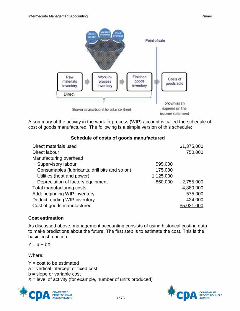
Cost flows used in manufacturing systems and the schedule of cost of goods manufactured
The following diagram illustrates the flows of costs through the various accounts used in a manufacturing system. Note the key accounts used to record these costs and the financial statements on which each account appears.
Intermediate Management Accounting Primer
3 / 73
A summary of the activity in the work-in-process (WIP) account is called the schedule of cost of goods manufactured. The following is a simple version of this schedule:
Schedule of costs of goods manufactured
Direct materials used $1,375,000
Direct labour 750,000
Manufacturing overhead
Supervisory labour 595,000
Consumables (lubricants, drill bits and so on) 175,000
Utilities (heat and power) 1,125,000
Depreciation of factory equipment 860,000 2,755,000
Total manufacturing costs 4,880,000
Add: beginning WIP inventory 575,000
Deduct: ending WIP inventory 424,000
Cost of goods manufactured $5,031,000
Cost estimation
As discussed above, management accounting consists of using historical costing data to make predictions about the future. The first step is to estimate the cost. This is the basic cost function:
Y = a + bX Where:
Y = cost to be estimated a = vertical intercept or fixed cost b = slope or variable cost X = level of activity (for example, number of units produced)
Intermediate Management Accounting Primer
4 / 73
There are a number of cost estimation methods including judgment and data approaches. Judgment approaches include engineering estimates, account analysis and the conference method, while data approaches include the high-low method, visual fit and statistical regression analysis. You may have covered many of these in your introductory course, so this primer will only touch on the statistical regression approach.
Statistical regression approach
The statistical regression approach fits an equation to the observed data using the criterion of minimizing the sum of the squared differences between the values predicted by the regression equation and the original data. The data is entered into a software package such as Microsoft Excel. The software then analyzes the data by applying regression analysis. The summary output provided by this tool consists of the following key regression statistics:
• The adjusted R-square (R2), which is a “best-fit” criterion also known as a goodness-of-fit measure (called the coefficient of determination). This measures the amount of variability in the dependent variable (Y) that is explained by changes in the independent variable (X).
• The estimated coefficients consisting of the intercept or fixed cost and the X variable or variable cost.
• The t-statistic, which is a formal statistical test of the hypothesis. For this course it can be assumed that, if the absolute value of the t-statistic is 2.00 or greater, a statistically significant relationship exists between the independent variable and the dependent variable.
There are several limitations of using historical costing data when making cost estimates. These limitations will be covered in the course.
Cost-volume-profit analysis
Managers use cost-volume-profit (CVP) analysis to assist in making decisions based on the relationship between costs and revenues and how changes in either affect the bottom line.
The CVP model
The basic CVP model is:
(Px) – (Vx) – F = OI

Intermediate Management Accounting Primer
5 / 73
Where:
P = selling price per unit V = variable cost per unit F = total fixed cost x = number of units produced and sold OI = operating income This equation allows the decision maker to answer a number of questions relating to profitability. One of these is the ability to identify the number of units (x) that must be made and sold to cover fixed costs (break-even point) and/or provide a target operating income. Contribution margin is the term used to identify how much revenue remains after deducting all variable costs. It is calculated as follows:
• Contribution margin (CM) per unit = P – V
• Contribution margin ratio = CM/P
Example Selling price: $4 per unit Variable costs: $2.50 per unit Fixed costs: $150,000 1. How many units must be sold to break even?
Using the CVP formula note that at break-even net income is $0. ($4x) – ($2.5x) – $150,000 = 0 Solve for x: $1.5x – $150,000 = 0 $1.5x = $150,000 x = $150,000 / $1.5 x = 100,000 units must be sold to break even. Break-even can also be calculated as follows: Break-even in units = F/CM = $150,000 / $1.5 = 100,000 units 2. How many units must be sold to earn a pre-tax operating income of
$100,000?
($4x) – ($2.5x) – $150,000 = $100,000
Intermediate Management Accounting Primer
6 / 73
Solve for x: $1.5x – $150,000 = $100,000 $1.5x = $250,000 x = $250,000 / $1.5x x = 166,667 units must be sold to earn a pre-tax operating income of $100,000. Achieving a target pre-tax operating income can also be calculated as follows: Units for target OI = (F + OI)/CM = ($150,000 + $100,000)/$1.5 = 166,667
Additionally, the break-even point or point to achieve desired income can be solved in dollars. Besides simply multiplying the break-even units by the selling price per unit, the CVP formula can be rewritten as follows:
Revenues to break even = F/CM ratio
For this example, CM ratio = 1.5/4 = 37.5%
$150,000 / 37.5% = $400,000 sales revenue is required to break even.
Revenues to achieved desired operating income = (F + OI)/CM ratio
For this example, ($150,000 +$100,000)/37.5% = $666,667 sales revenue is required to achieve the target operating income. Note that this is an estimate. If 166,667 units are required, then in dollars this would be 166,667 × $4 = $666,668. Also, note that you can’t sell part units so the number of units to break even must always be rounded up to the nearest whole number.
Taxes and the CVP equation
If taxes are to be considered, the CVP equation is expressed as follows: Units for target NI = {F + [NI / (1 – tax rate)]} / CM Operating income = NI / (1 – tax rate) Where after-tax net income = [(Px – Vx) – F] × (1 – tax rate)
Example Selling price: $4 per unit Variable costs: $2.50 per unit Fixed costs: $150,000 Tax rate: 30% How many units must be sold to earn an after-tax net income of $100,000? {F + [NI / (1 – tax rate)]} / CM {$150,000 + [$100,000 / (1 – 0.3)]} / $1.50 ($150,000 + $142,857.16)/$1.50 = 195,239 units (rounded up)

Intermediate Management Accounting Primer
7 / 73
Multi-product CVP analysis
CVP analysis can be used where a company produces and sells more than one product. In those situations, the units are combined in a bundle based on the projected sales mix. The contribution margin of the bundle is the denominator of the break-even equation while the numerator is the total fixed costs. As with calculating unit break-even point, bundle break-even is always rounded up to the nearest complete bundle. Once the break-even in sales mix bundles has been determined, the bundles are broken apart and each product in the mix is multiplied by the number of bundles.
Example Product A (200 units) Product B (100 units)
Per unit Total Per unit Total Firm total
Revenue $100 $20,000 $ 250 $ 25,000 $ 45,000
Variable cost 40 8,000 100 10,000 18,000
Contribution margin
$ 60 $12,000 $ 150 $ 15,000 $ 27,000
Fixed cost 21,600
Operating income $ 5,400
The sales mix based on the sales volume is: two units of Product A are sold for every unit of Product B. 200:100 = 2:1 The contribution margin using the sales mix is:
(2 × $60) + (1 × $150) = $270 per bundle of product
Then use the F/CM equation to arrive at the break-even bundles: $21,600 / $270 = 80 bundles. Each bundle consists of two units of Product A and one unit of Product B.
(2 × 80) = 160 units of Product A (1 × 80) = 80 units of Product B
Practice questions
1. Multiple-choice questions: i. The following selected data from April were taken from Elfin Inc.’s financial
statements:
Cost of goods available for sale $ 79,000 Manufacturing overhead 20,000 Cost of goods manufactured 69,000 Finished goods inventory — beginning 10,000 Direct materials used 16,000 Sales 130,000 Direct labour 23,000
Intermediate Management Accounting Primer
8 / 73
WIP inventory — beginning 15,000 Cost of goods sold 71,000
What was the WIP inventory at the end of April?
a) $5,000 b) $10,000 c) $15,000 d) $44,000
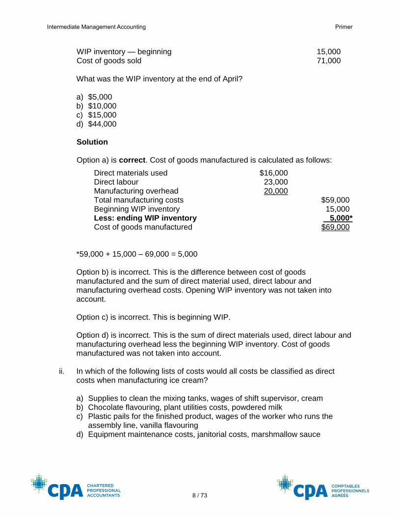
Solution Option a) is correct. Cost of goods manufactured is calculated as follows:
Direct materials used $16,000 Direct labour 23,000 Manufacturing overhead 20,000 Total manufacturing costs $59,000 Beginning WIP inventory 15,000 Less: ending WIP inventory 5,000* Cost of goods manufactured $69,000 *59,000 + 15,000 – 69,000 = 5,000 Option b) is incorrect. This is the difference between cost of goods manufactured and the sum of direct material used, direct labour and manufacturing overhead costs. Opening WIP inventory was not taken into account. Option c) is incorrect. This is beginning WIP. Option d) is incorrect. This is the sum of direct materials used, direct labour and manufacturing overhead less the beginning WIP inventory. Cost of goods manufactured was not taken into account.
ii. In which of the following lists of costs would all costs be classified as direct costs when manufacturing ice cream?
a) Supplies to clean the mixing tanks, wages of shift supervisor, cream b) Chocolate flavouring, plant utilities costs, powdered milk c) Plastic pails for the finished product, wages of the worker who runs the
assembly line, vanilla flavouring d) Equipment maintenance costs, janitorial costs, marshmallow sauce
Intermediate Management Accounting Primer
9 / 73
Solution Option c) is correct. Plastic pails and vanilla flavouring are direct ingredients and the wages of the worker who runs the assembly line is direct labour. Option a) is incorrect. Both the supplies to clean the mixing tanks and the wages of the shift supervisor are manufacturing overhead costs. Option b) is incorrect. The plant utilities costs are a manufacturing overhead cost. Option d) is incorrect. Both equipment maintenance and janitorial costs are manufacturing overhead costs.
2. ALF Inc. is starting to manufacture metal desks. It has been determined that the market demand can be 7,000, 8,000 or 9,000 units. To start up, ALF obtained a $3 million term loan at 6%. Other information is as follows:
Selling price per desk $200 Variable cost per desk $50 Total fixed costs $1,000,000 (includes interest on the term loan)
Required:
a) What is ALF’s break-even point in units and in dollars?
b) There is a risk that ALF may have to take out an additional loan for $1,500,000 at the same rate as its current loan. If so, what is the minimum level of demand (7,000, 8,000 or 9,000 units) at which ALF must operate?
Solution
a) CPA Way step: Assess the Situation
Break-even in units = $1,000,000 ÷ ($200 – $50) = 6,667 units Break-even in sales dollars = $1,000,000 ÷ [($200 – $50) ÷ $200] = $1,333,333 Or 6,667 units × $200 = $1,333,400
b) CPA Way steps: Analyze Major Issue(s) and Conclude and Advise
An additional loan of $1,500,000 at 6% annual interest will require $1,500,000 × 0.06 = $90,000 in additional profits to pay the interest. ($1,000,000 + $90,000) / ($200 – $50) = 7,267 units Thus ALF must operate at a minimum level of 8,000 units to pay the loan interest.
Intermediate Management Accounting Primer
10 / 73
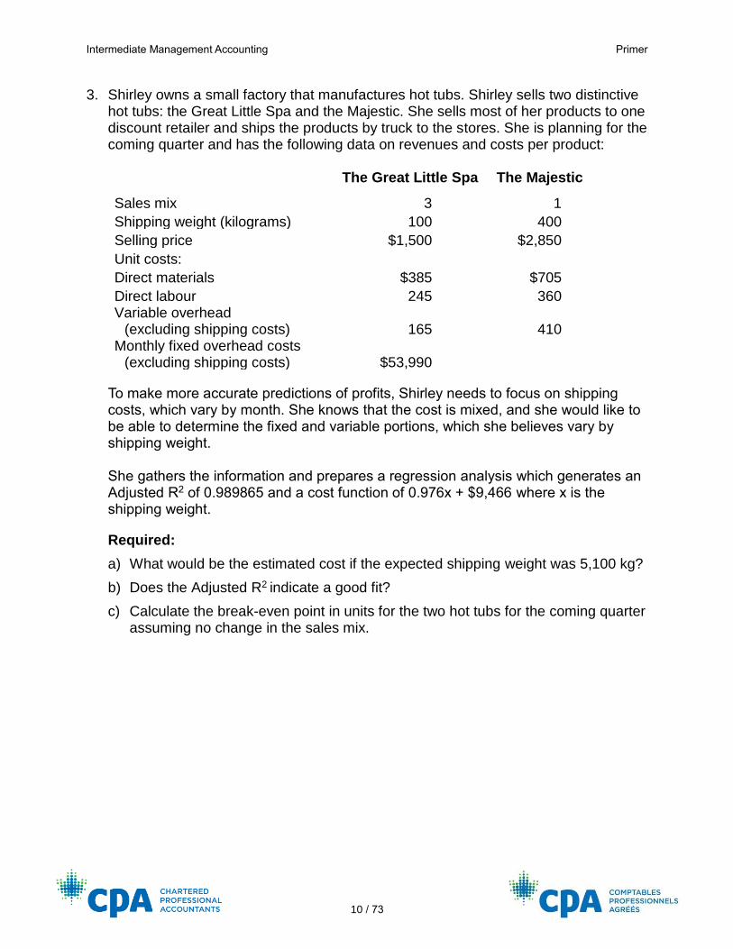
3. Shirley owns a small factory that manufactures hot tubs. Shirley sells two distinctive hot tubs: the Great Little Spa and the Majestic. She sells most of her products to one discount retailer and ships the products by truck to the stores. She is planning for the coming quarter and has the following data on revenues and costs per product:
The Great Little Spa The Majestic
Sales mix 3 1
Shipping weight (kilograms) 100 400
Selling price $1,500 $2,850
Unit costs: Direct materials $385 $705
Direct labour 245 360 Variable overhead
(excluding shipping costs) 165 410 Monthly fixed overhead costs
(excluding shipping costs) $53,990
To make more accurate predictions of profits, Shirley needs to focus on shipping costs, which vary by month. She knows that the cost is mixed, and she would like to be able to determine the fixed and variable portions, which she believes vary by shipping weight. She gathers the information and prepares a regression analysis which generates an Adjusted R2 of 0.989865 and a cost function of 0.976x + $9,466 where x is the shipping weight.
Required:
a) What would be the estimated cost if the expected shipping weight was 5,100 kg?
b) Does the Adjusted R2 indicate a good fit?
c) Calculate the break-even point in units for the two hot tubs for the coming quarter assuming no change in the sales mix.
Intermediate Management Accounting Primer
11 / 73
Solution
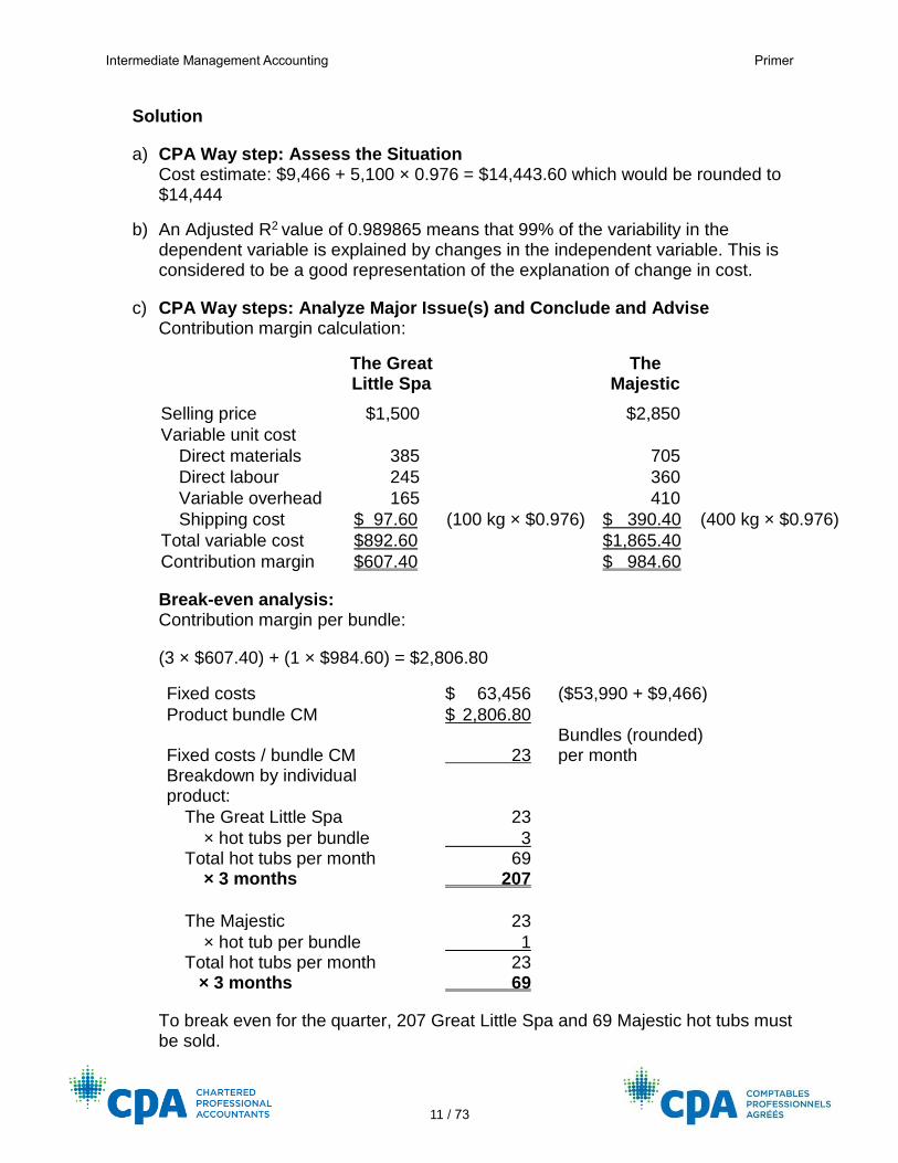
a) CPA Way step: Assess the Situation Cost estimate: $9,466 + 5,100 × 0.976 = $14,443.60 which would be rounded to $14,444
b) An Adjusted R2 value of 0.989865 means that 99% of the variability in the dependent variable is explained by changes in the independent variable. This is considered to be a good representation of the explanation of change in cost.
c) CPA Way steps: Analyze Major Issue(s) and Conclude and Advise Contribution margin calculation:
The Great Little Spa
The Majestic
Selling price $1,500 $2,850
Variable unit cost
Direct materials 385 705
Direct labour 245 360
Variable overhead 165 410
Shipping cost $ 97.60 (100 kg × $0.976) $ 390.40 (400 kg × $0.976)
Total variable cost $892.60 $1,865.40
Contribution margin $607.40 $ 984.60
Break-even analysis: Contribution margin per bundle:
(3 × $607.40) + (1 × $984.60) = $2,806.80
Fixed costs $ 63,456 ($53,990 + $9,466)
Product bundle CM $ 2,806.80
Fixed costs / bundle CM 23 Bundles (rounded) per month
Breakdown by individual product:
The Great Little Spa 23
× hot tubs per bundle 3 Total hot tubs per month
× 3 months 69 207
The Majestic 23
× hot tub per bundle 1 Total hot tubs per month
× 3 months 23 69
To break even for the quarter, 207 Great Little Spa and 69 Majestic hot tubs must be sold.
Intermediate Management Accounting Primer
12 / 73
PART 2: CAPACITY
Manufacturing capacity is the constraint on the amount of resources that are available to manufacture a product or provide a service. Actual, normal, theoretical and practical capacity are some of the ways of valuing capacity. Typically, the greater the capacity, the greater the related fixed costs. Managing the use of capacity, therefore, allows companies to manage related fixed costs.
Support department cost allocation
Support (or service) departments assist production departments by providing resources that the production departments need to complete their work. The main reason that the costs of these departments are allocated to the production departments is to help organizations have a better understanding of the costs of all resources needed to produce a good (product or service). Common examples of support departments include accounting, legal, administrative and human resources. Three different methods can be used to allocate support department costs to production departments.
Allocation methods
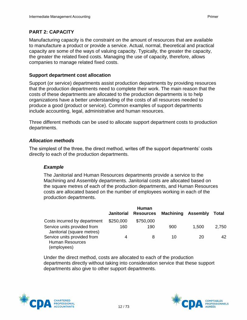
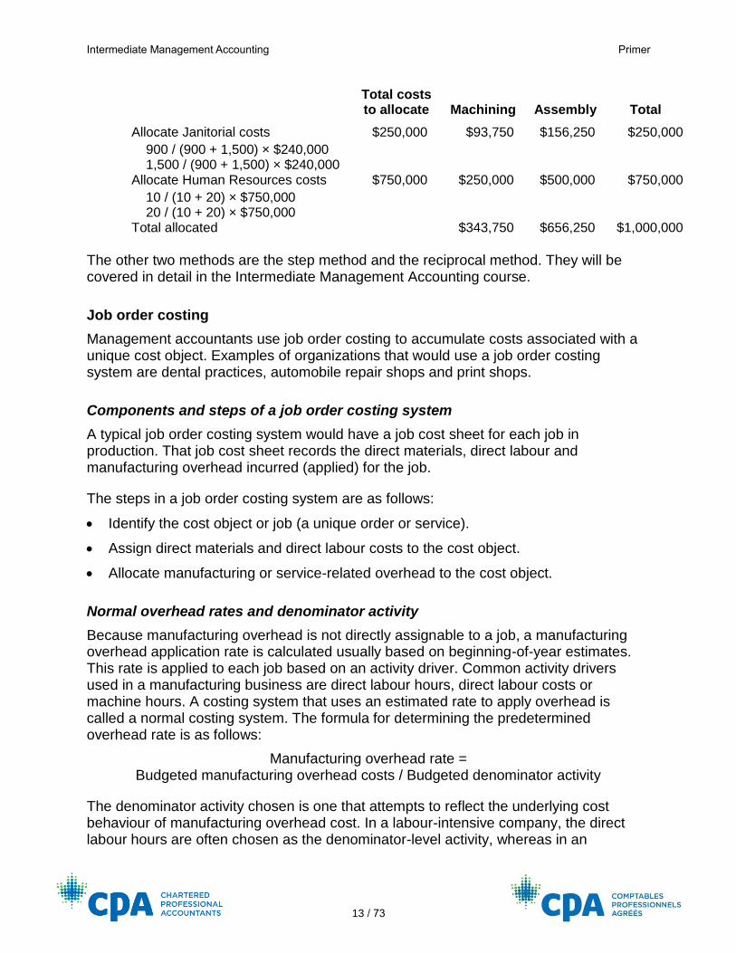
The simplest of the three, the direct method, writes off the support departments’ costs directly to each of the production departments.
Example
The Janitorial and Human Resources departments provide a service to the Machining and Assembly departments. Janitorial costs are allocated based on the square metres of each of the production departments, and Human Resources costs are allocated based on the number of employees working in each of the production departments.
Janitorial Human
Resources Machining Assembly Total
Costs incurred by department $250,000 $750,000
Service units provided from Janitorial (square metres)
160 190 900 1,500 2,750
Service units provided from Human Resources (employees)
4 8 10 20 42
Under the direct method, costs are allocated to each of the production departments directly without taking into consideration service that these support departments also give to other support departments.
Intermediate Management Accounting Primer
13 / 73
Total costs to allocate Machining Assembly Total
Allocate Janitorial costs $250,000 $93,750 $156,250 $250,000
900 / (900 + 1,500) × $240,000 1,500 / (900 + 1,500) × $240,000
Allocate Human Resources costs $750,000 $250,000 $500,000 $750,000
10 / (10 + 20) × $750,000 20 / (10 + 20) × $750,000
Total allocated
$343,750 $656,250 $1,000,000
The other two methods are the step method and the reciprocal method. They will be covered in detail in the Intermediate Management Accounting course.
Job order costing
Management accountants use job order costing to accumulate costs associated with a unique cost object. Examples of organizations that would use a job order costing system are dental practices, automobile repair shops and print shops.
Components and steps of a job order costing system
A typical job order costing system would have a job cost sheet for each job in production. That job cost sheet records the direct materials, direct labour and manufacturing overhead incurred (applied) for the job.
The steps in a job order costing system are as follows:
• Identify the cost object or job (a unique order or service).
• Assign direct materials and direct labour costs to the cost object.
• Allocate manufacturing or service-related overhead to the cost object.
Normal overhead rates and denominator activity
Because manufacturing overhead is not directly assignable to a job, a manufacturing overhead application rate is calculated usually based on beginning-of-year estimates. This rate is applied to each job based on an activity driver. Common activity drivers used in a manufacturing business are direct labour hours, direct labour costs or machine hours. A costing system that uses an estimated rate to apply overhead is called a normal costing system. The formula for determining the predetermined overhead rate is as follows:
Manufacturing overhead rate = Budgeted manufacturing overhead costs / Budgeted denominator activity
The denominator activity chosen is one that attempts to reflect the underlying cost behaviour of manufacturing overhead cost. In a labour-intensive company, the direct labour hours are often chosen as the denominator-level activity, whereas in an
Intermediate Management Accounting Primer
14 / 73
automated company, machine hours are usually chosen. Common choices for activity level are historic actual, estimated, average, and practical capacity of the cost driver.
The amount of manufacturing overhead applied to a job will equal the manufacturing overhead rate multiplied by the actual denominator activity specific to the job.
Single plant-wide versus multiple overhead cost pools
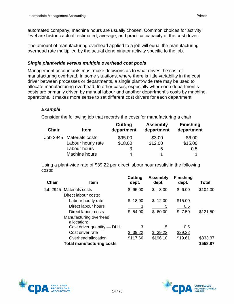
Management accountants must make decisions as to what drives the cost of manufacturing overhead. In some situations, where there is little variability in the cost driver between processes or departments, a single plant-wide rate may be used to allocate manufacturing overhead. In other cases, especially where one department’s costs are primarily driven by manual labour and another department’s costs by machine operations, it makes more sense to set different cost drivers for each department.
Example
Consider the following job that records the costs for manufacturing a chair:
Chair Item Cutting
department Assembly
department Finishing
department
Job 2945 Materials costs $95.00 $3.00 $6.00 Labour hourly rate $18.00 $12.00 $15.00 Labour hours 3 5 0.5 Machine hours 4 1 1
Using a plant-wide rate of $39.22 per direct labour hour results in the following costs:
Chair Item Cutting dept.
Assembly dept.
Finishing dept. Total
Job 2945 Materials costs $ 95.00 $ 3.00 $ 6.00 $104.00
Direct labour costs: Labour hourly rate $ 18.00 $ 12.00 $15.00
Direct labour hours 3 5 0.5
Direct labour costs $ 54.00 $ 60.00 $ 7.50 $121.50
Manufacturing overhead allocation:
Cost driver quantity — DLH 3 5 0.5
Cost driver rate $ 39.22 $ 39.22 $39.22
Overhead allocation $117.66 $196.10 $19.61 $333.37 Total manufacturing costs $558.87
Intermediate Management Accounting Primer
15 / 73
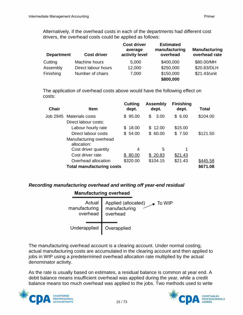
Alternatively, if the overhead costs in each of the departments had different cost drivers, the overhead costs could be applied as follows:
Department Cost driver
Cost driver average
activity level
Estimated manufacturing
overhead Manufacturing overhead rate
Cutting Machine hours 5,000 $400,000 $80.00/MH
Assembly Direct labour hours 12,000 $250,000 $20.83/DLH
Finishing Number of chairs 7,000 $150,000 $21.43/unit $800,000
The application of overhead costs above would have the following effect on costs:
Chair Item Cutting dept.
Assembly dept.
Finishing dept. Total
Job 2945 Materials costs $ 95.00 $ 3.00 $ 6.00 $104.00 Direct labour costs:
Labour hourly rate $ 18.00 $ 12.00 $15.00
Direct labour costs $ 54.00 $ 60.00 $ 7.50 $121.50
Manufacturing overhead allocation:
Cost driver quantity 4 5 1
Cost driver rate $ 80.00 $ 20.83 $21.43
Overhead allocation $320.00 $104.15 $21.43 $445.58
Total manufacturing costs $671.08
Recording manufacturing overhead and writing off year-end residual
The manufacturing overhead account is a clearing account. Under normal costing, actual manufacturing costs are accumulated in the clearing account and then applied to jobs in WIP using a predetermined overhead allocation rate multiplied by the actual denominator activity.
As the rate is usually based on estimates, a residual balance is common at year end. A debit balance means insufficient overhead was applied during the year, while a credit balance means too much overhead was applied to the jobs. Two methods used to write
Actual manufacturing
overhead
Manufacturing overhead
Underapplied
Applied (allocated) manufacturing overhead
Overapplied
To WIP
Intermediate Management Accounting Primer
16 / 73
off this amount are the direct charge to cost of goods sold method and the prorating based on ending balances method.
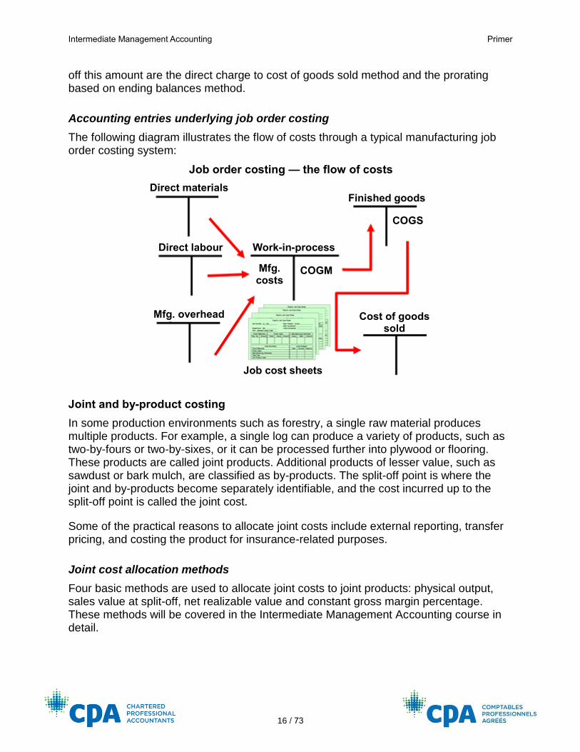
Accounting entries underlying job order costing
The following diagram illustrates the flow of costs through a typical manufacturing job order costing system:
Joint and by-product costing
In some production environments such as forestry, a single raw material produces multiple products. For example, a single log can produce a variety of products, such as two-by-fours or two-by-sixes, or it can be processed further into plywood or flooring. These products are called joint products. Additional products of lesser value, such as sawdust or bark mulch, are classified as by-products. The split-off point is where the joint and by-products become separately identifiable, and the cost incurred up to the split-off point is called the joint cost.
Some of the practical reasons to allocate joint costs include external reporting, transfer pricing, and costing the product for insurance-related purposes.
Joint cost allocation methods
Four basic methods are used to allocate joint costs to joint products: physical output, sales value at split-off, net realizable value and constant gross margin percentage. These methods will be covered in the Intermediate Management Accounting course in detail.
Direct materials
Job order costing — the flow of costs
Finished goods
Direct labour Work-in-process
Mfg. costs
Mfg. overhead
Job cost sheets
Cost of goods sold
COGM
COGS
Intermediate Management Accounting Primer
17 / 73
Practice questions
1. Multiple-choice questions:
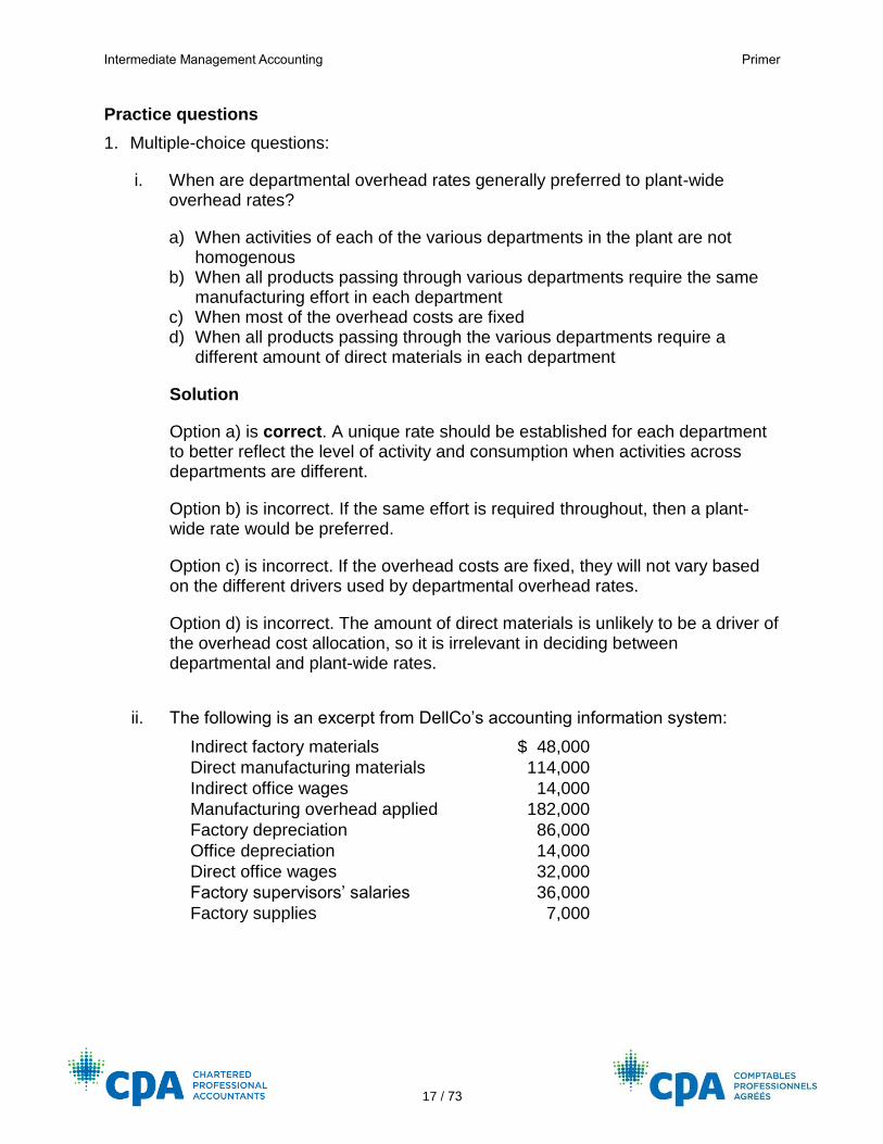
i. When are departmental overhead rates generally preferred to plant-wide overhead rates?
a) When activities of each of the various departments in the plant are not homogenous
b) When all products passing through various departments require the same manufacturing effort in each department
c) When most of the overhead costs are fixed d) When all products passing through the various departments require a
different amount of direct materials in each department
Solution
Option a) is correct. A unique rate should be established for each department to better reflect the level of activity and consumption when activities across departments are different.
Option b) is incorrect. If the same effort is required throughout, then a plant-wide rate would be preferred.
Option c) is incorrect. If the overhead costs are fixed, they will not vary based on the different drivers used by departmental overhead rates.
Option d) is incorrect. The amount of direct materials is unlikely to be a driver of the overhead cost allocation, so it is irrelevant in deciding between departmental and plant-wide rates.
ii. The following is an excerpt from DellCo’s accounting information system:
Indirect factory materials $ 48,000
Direct manufacturing materials 114,000
Indirect office wages 14,000
Manufacturing overhead applied 182,000
Factory depreciation 86,000
Office depreciation 14,000
Direct office wages 32,000
Factory supervisors’ salaries 36,000
Factory supplies 7,000
Intermediate Management Accounting Primer
18 / 73
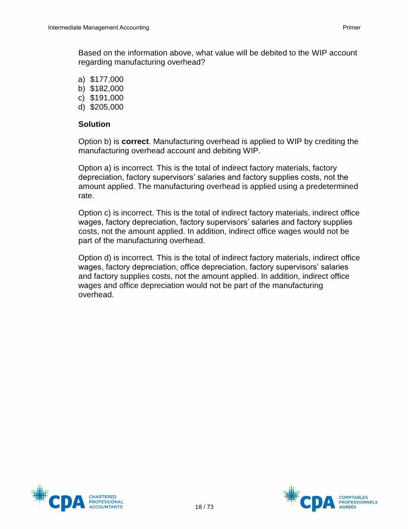
Based on the information above, what value will be debited to the WIP account regarding manufacturing overhead?
a) $177,000 b) $182,000 c) $191,000 d) $205,000
Solution
Option b) is correct. Manufacturing overhead is applied to WIP by crediting the manufacturing overhead account and debiting WIP.
Option a) is incorrect. This is the total of indirect factory materials, factory depreciation, factory supervisors’ salaries and factory supplies costs, not the amount applied. The manufacturing overhead is applied using a predetermined rate.
Option c) is incorrect. This is the total of indirect factory materials, indirect office wages, factory depreciation, factory supervisors’ salaries and factory supplies costs, not the amount applied. In addition, indirect office wages would not be part of the manufacturing overhead.
Option d) is incorrect. This is the total of indirect factory materials, indirect office wages, factory depreciation, office depreciation, factory supervisors’ salaries and factory supplies costs, not the amount applied. In addition, indirect office wages and office depreciation would not be part of the manufacturing overhead.
Intermediate Management Accounting Primer
19 / 73
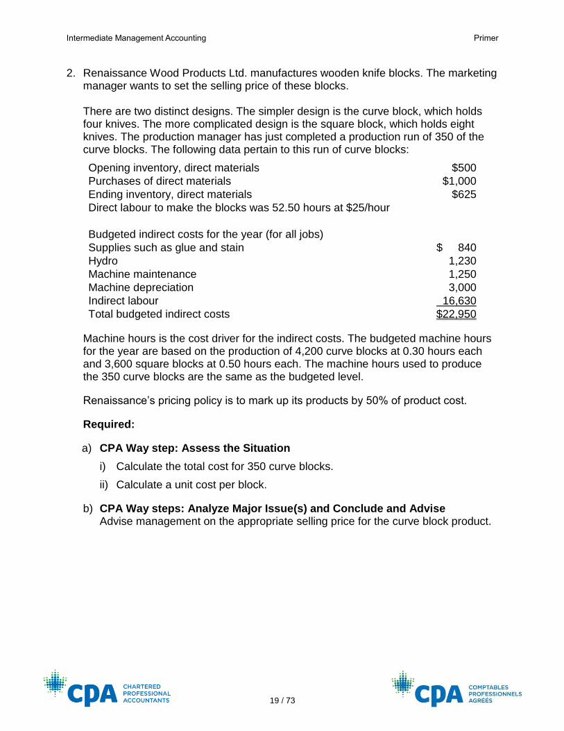
2. Renaissance Wood Products Ltd. manufactures wooden knife blocks. The marketing manager wants to set the selling price of these blocks. There are two distinct designs. The simpler design is the curve block, which holds four knives. The more complicated design is the square block, which holds eight knives. The production manager has just completed a production run of 350 of the curve blocks. The following data pertain to this run of curve blocks:
Opening inventory, direct materials $500
Purchases of direct materials $1,000
Ending inventory, direct materials $625
Direct labour to make the blocks was 52.50 hours at $25/hour
Budgeted indirect costs for the year (for all jobs)
Supplies such as glue and stain $ 840
Hydro 1,230
Machine maintenance 1,250
Machine depreciation 3,000
Indirect labour 16,630
Total budgeted indirect costs $22,950
Machine hours is the cost driver for the indirect costs. The budgeted machine hours for the year are based on the production of 4,200 curve blocks at 0.30 hours each and 3,600 square blocks at 0.50 hours each. The machine hours used to produce the 350 curve blocks are the same as the budgeted level.
Renaissance’s pricing policy is to mark up its products by 50% of product cost.
Required:
a) CPA Way step: Assess the Situation
i) Calculate the total cost for 350 curve blocks.
ii) Calculate a unit cost per block.
b) CPA Way steps: Analyze Major Issue(s) and Conclude and Advise Advise management on the appropriate selling price for the curve block product.
Intermediate Management Accounting Primer
20 / 73
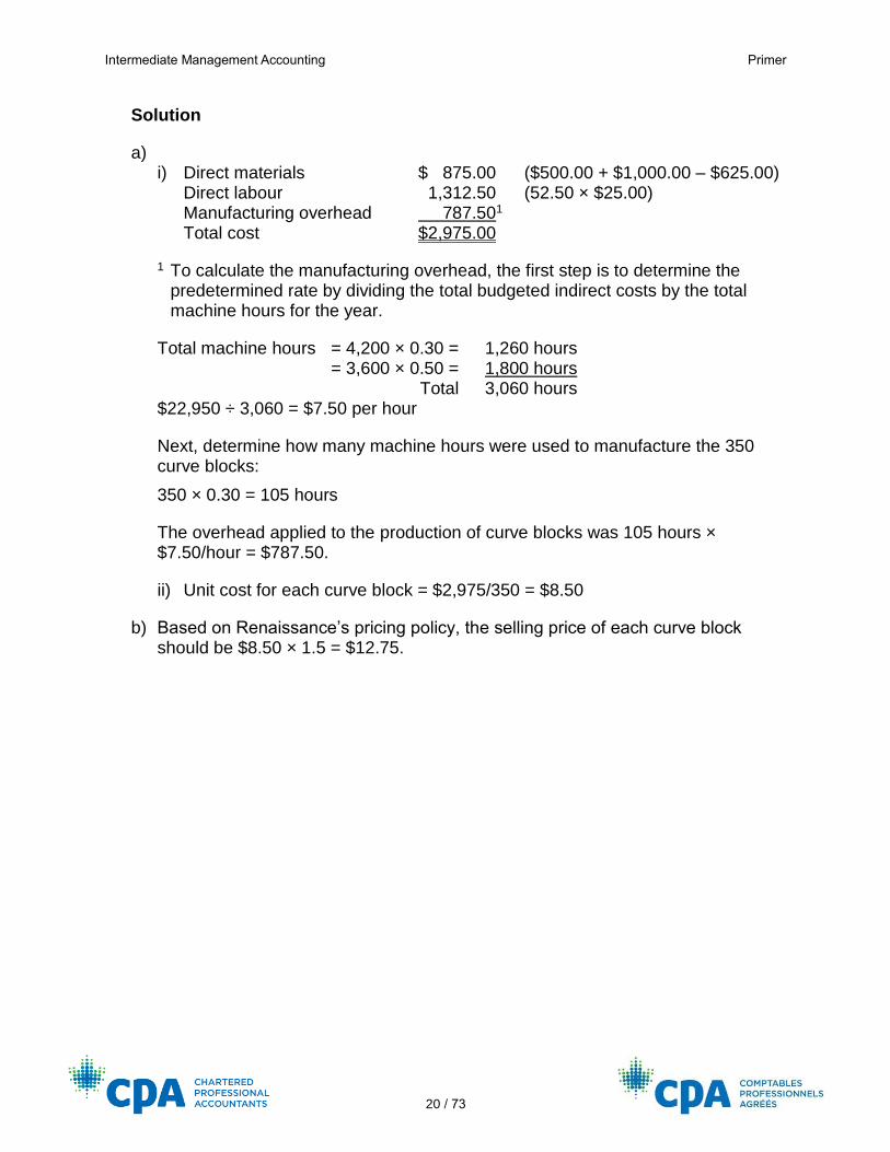
Solution
a) i) Direct materials $ 875.00 ($500.00 + $1,000.00 – $625.00) Direct labour 1,312.50 (52.50 × $25.00) Manufacturing overhead 787.501 Total cost $2,975.00
1 To calculate the manufacturing overhead, the first step is to determine the predetermined rate by dividing the total budgeted indirect costs by the total machine hours for the year.
Total machine hours = 4,200 × 0.30 = 1,260 hours = 3,600 × 0.50 = 1,800 hours Total 3,060 hours $22,950 ÷ 3,060 = $7.50 per hour
Next, determine how many machine hours were used to manufacture the 350 curve blocks:
350 × 0.30 = 105 hours
The overhead applied to the production of curve blocks was 105 hours × $7.50/hour = $787.50.
ii) Unit cost for each curve block = $2,975/350 = $8.50
b) Based on Renaissance’s pricing policy, the selling price of each curve block should be $8.50 × 1.5 = $12.75.
Intermediate Management Accounting Primer
21 / 73
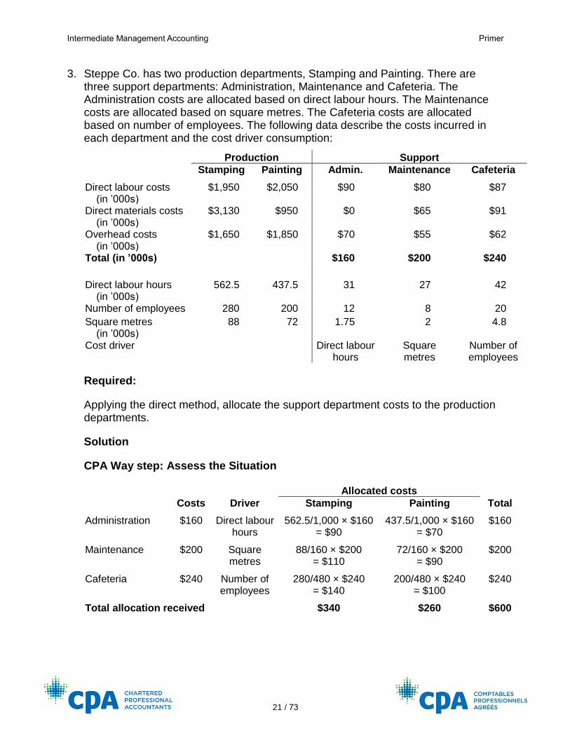
3. Steppe Co. has two production departments, Stamping and Painting. There are three support departments: Administration, Maintenance and Cafeteria. The Administration costs are allocated based on direct labour hours. The Maintenance costs are allocated based on square metres. The Cafeteria costs are allocated based on number of employees. The following data describe the costs incurred in each department and the cost driver consumption:
Production Support
Stamping Painting Admin. Maintenance Cafeteria
Direct labour costs (in ’000s)
$1,950 $2,050 $90 $80 $87
Direct materials costs (in ’000s)
$3,130 $950 $0 $65 $91
Overhead costs (in ’000s)
$1,650 $1,850 $70 $55 $62
Total (in ’000s) $160 $200 $240
Direct labour hours (in ’000s)
562.5 437.5 31 27 42
Number of employees 280 200 12 8 20
Square metres (in ’000s)
88 72 1.75 2 4.8
Cost driver Direct labour hours
Square metres
Number of employees
Required:
Applying the direct method, allocate the support department costs to the production departments.
Solution
CPA Way step: Assess the Situation
Allocated costs
Costs Driver Stamping Painting Total
Administration $160 Direct labour hours
562.5/1,000 × $160 = $90
437.5/1,000 × $160 = $70
$160
Maintenance $200 Square metres
88/160 × $200 = $110
72/160 × $200 = $90
$200
Cafeteria $240 Number of employees
280/480 × $240 = $140
200/480 × $240 = $100
$240
Total allocation received $340 $260 $600
Intermediate Management Accounting Primer
22 / 73
PART 3: PROCESS COSTING
Process costing is a costing system suitable for costing the mass production of identical products (for example, packaging soft drinks and manufacturing plastic bottles). Instead of costing individual units or jobs as is done in job costing, total costs are simply divided by the number of units produced to compute the cost per unit. The purpose of job and process costing is to cost products and services. However, some of the differences are as follows:
Job order costing Process costing
Products Each product is unique. Each product is the same as all others.
Cost accumulation Costs are collected and recorded for each job.
Costs are collected and recorded by department/process.
Reporting of costs Costs are accumulated and reported on the job cost sheet.
Costs are reported on the department production report.
Unit costs Unit costs are calculated for each job.
Unit costs are calculated for each department.
Illustration of a typical process costing system at a soft drink manufacturing plant
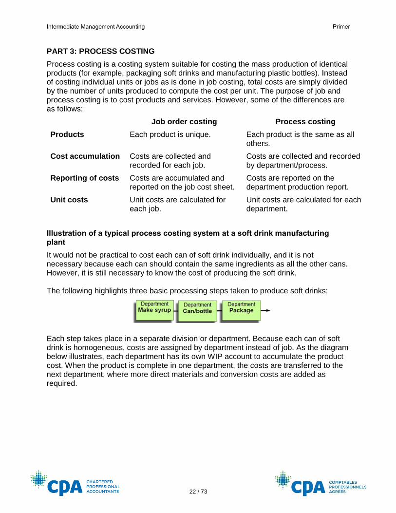
It would not be practical to cost each can of soft drink individually, and it is not necessary because each can should contain the same ingredients as all the other cans. However, it is still necessary to know the cost of producing the soft drink. The following highlights three basic processing steps taken to produce soft drinks:
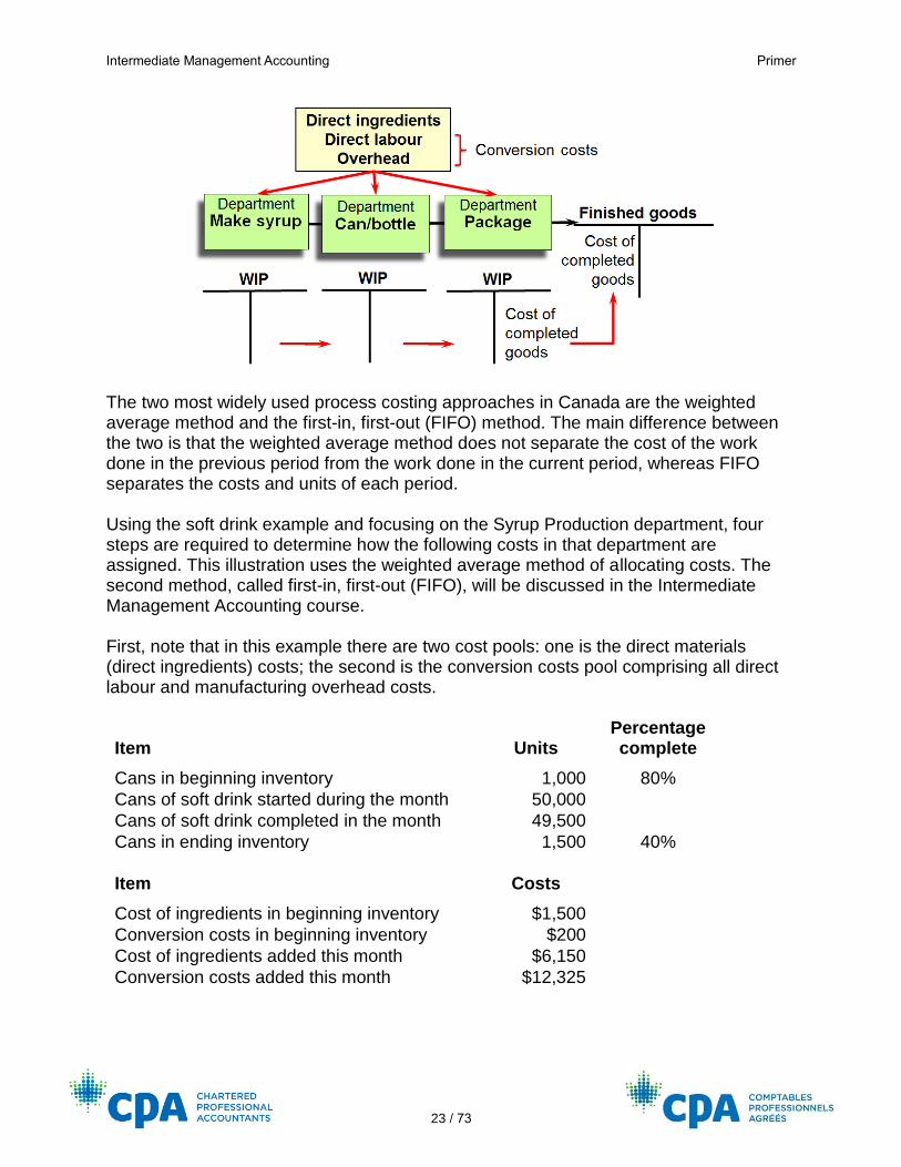
Each step takes place in a separate division or department. Because each can of soft drink is homogeneous, costs are assigned by department instead of job. As the diagram below illustrates, each department has its own WIP account to accumulate the product cost. When the product is complete in one department, the costs are transferred to the next department, where more direct materials and conversion costs are added as required.
Intermediate Management Accounting Primer
23 / 73
The two most widely used process costing approaches in Canada are the weighted average method and the first-in, first-out (FIFO) method. The main difference between the two is that the weighted average method does not separate the cost of the work done in the previous period from the work done in the current period, whereas FIFO separates the costs and units of each period. Using the soft drink example and focusing on the Syrup Production department, four steps are required to determine how the following costs in that department are assigned. This illustration uses the weighted average method of allocating costs. The second method, called first-in, first-out (FIFO), will be discussed in the Intermediate Management Accounting course. First, note that in this example there are two cost pools: one is the direct materials (direct ingredients) costs; the second is the conversion costs pool comprising all direct labour and manufacturing overhead costs.
Item Units Percentage complete
Cans in beginning inventory 1,000 80%
Cans of soft drink started during the month 50,000 Cans of soft drink completed in the month 49,500 Cans in ending inventory 1,500 40%
Item Costs
Cost of ingredients in beginning inventory $1,500 Conversion costs in beginning inventory $200 Cost of ingredients added this month $6,150 Conversion costs added this month $12,325
Intermediate Management Accounting Primer
24 / 73
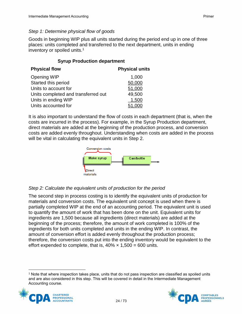
Step 1: Determine physical flow of goods
Goods in beginning WIP plus all units started during the period end up in one of three places: units completed and transferred to the next department, units in ending inventory or spoiled units.1
Syrup Production department
Physical flow Physical units
Opening WIP 1,000
Started this period 50,000
Units to account for 51,000
Units completed and transferred out 49,500
Units in ending WIP 1,500
Units accounted for 51,000 It is also important to understand the flow of costs in each department (that is, when the costs are incurred in the process). For example, in the Syrup Production department, direct materials are added at the beginning of the production process, and conversion costs are added evenly throughout. Understanding when costs are added in the process will be vital in calculating the equivalent units in Step 2.
Step 2: Calculate the equivalent units of production for the period
The second step in process costing is to identify the equivalent units of production for materials and conversion costs. The equivalent unit concept is used when there is partially completed WIP at the end of an accounting period. The equivalent unit is used to quantify the amount of work that has been done on the unit. Equivalent units for ingredients are 1,500 because all ingredients (direct materials) are added at the beginning of the process; therefore, the amount of work completed is 100% of the ingredients for both units completed and units in the ending WIP. In contrast, the amount of conversion effort is added evenly throughout the production process; therefore, the conversion costs put into the ending inventory would be equivalent to the effort expended to complete, that is, 40% × 1,500 = 600 units.
1 Note that where inspection takes place, units that do not pass inspection are classified as spoiled units and are also considered in this step. This will be covered in detail in the Intermediate Management Accounting course.
Intermediate Management Accounting Primer
25 / 73
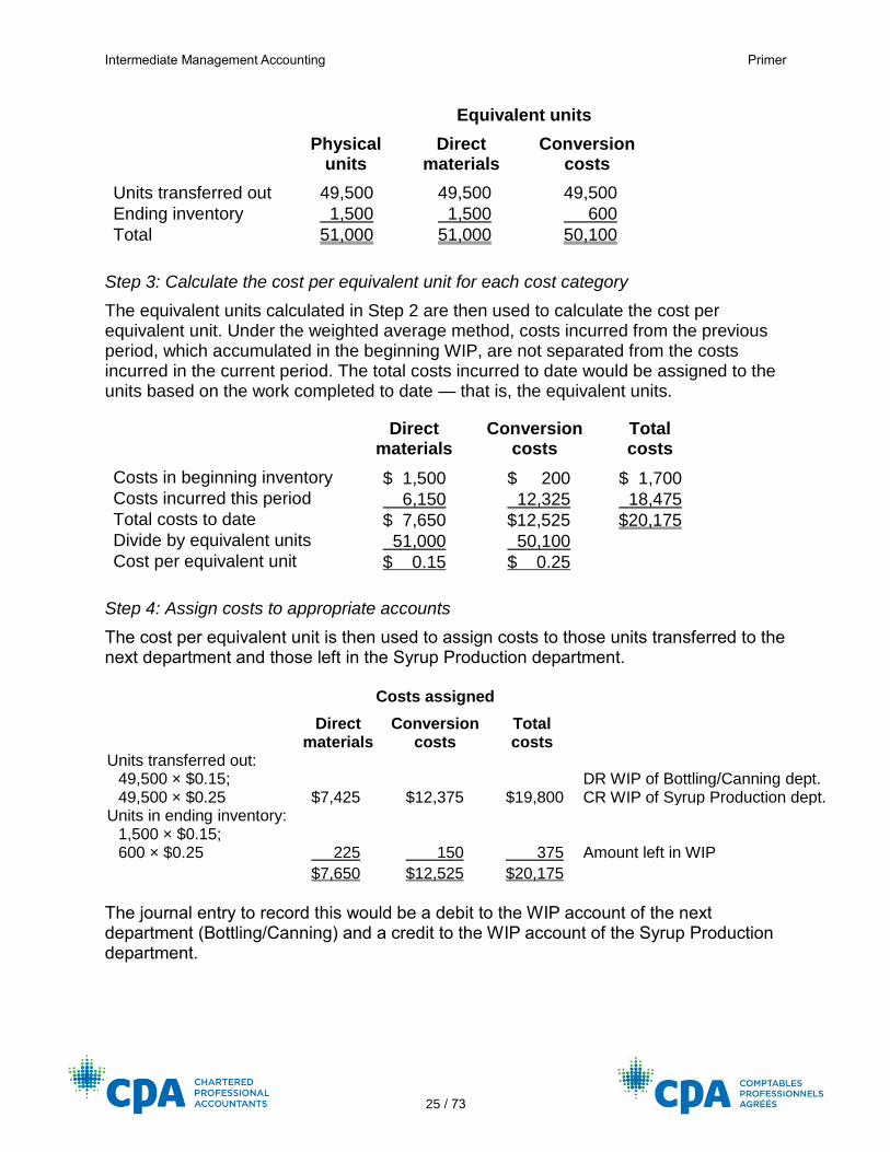
Physical units
Equivalent units
Direct materials
Conversion costs
Units transferred out 49,500 49,500 49,500
Ending inventory 1,500 1,500 600
Total 51,000 51,000 50,100
Step 3: Calculate the cost per equivalent unit for each cost category
The equivalent units calculated in Step 2 are then used to calculate the cost per equivalent unit. Under the weighted average method, costs incurred from the previous period, which accumulated in the beginning WIP, are not separated from the costs incurred in the current period. The total costs incurred to date would be assigned to the units based on the work completed to date — that is, the equivalent units.
Direct materials
Conversion costs
Total costs
Costs in beginning inventory $ 1,500 $ 200 $ 1,700 Costs incurred this period 6,150 12,325 18,475 Total costs to date $ 7,650 $12,525 $20,175 Divide by equivalent units 51,000 50,100 Cost per equivalent unit $ 0.15 $ 0.25
Step 4: Assign costs to appropriate accounts
The cost per equivalent unit is then used to assign costs to those units transferred to the next department and those left in the Syrup Production department.
Costs assigned
Direct materials
Conversion costs
Total costs
Units transferred out: 49,500 × $0.15; 49,500 × $0.25 $7,425 $12,375 $19,800
DR WIP of Bottling/Canning dept. CR WIP of Syrup Production dept.
Units in ending inventory: 1,500 × $0.15; 600 × $0.25 225 150 375 Amount left in WIP
$7,650 $12,525 $20,175 The journal entry to record this would be a debit to the WIP account of the next department (Bottling/Canning) and a credit to the WIP account of the Syrup Production department.
Intermediate Management Accounting Primer
26 / 73
Spoilage
Spoilage is identified at a point of inspection and can be classified as either abnormal or normal. Abnormal spoilage is spoiled units above the number that is expected or normal for the process. Normal spoilage contributes to the cost of the good units produced, whereas abnormal spoilage is reported as a period cost in the period incurred. The cost of spoiled units is based on the percentage of completion at the point where the units were inspected.
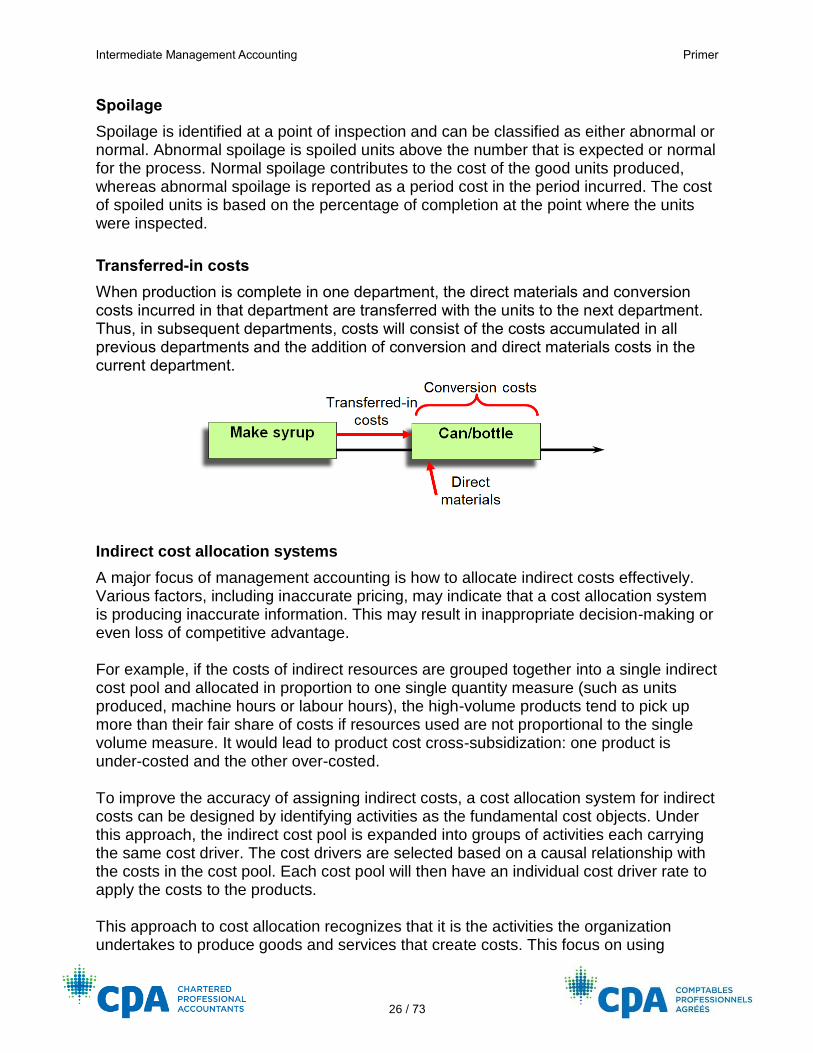
Transferred-in costs
When production is complete in one department, the direct materials and conversion costs incurred in that department are transferred with the units to the next department. Thus, in subsequent departments, costs will consist of the costs accumulated in all previous departments and the addition of conversion and direct materials costs in the current department.
Indirect cost allocation systems
A major focus of management accounting is how to allocate indirect costs effectively. Various factors, including inaccurate pricing, may indicate that a cost allocation system is producing inaccurate information. This may result in inappropriate decision-making or even loss of competitive advantage. For example, if the costs of indirect resources are grouped together into a single indirect cost pool and allocated in proportion to one single quantity measure (such as units produced, machine hours or labour hours), the high-volume products tend to pick up more than their fair share of costs if resources used are not proportional to the single volume measure. It would lead to product cost cross-subsidization: one product is under-costed and the other over-costed. To improve the accuracy of assigning indirect costs, a cost allocation system for indirect costs can be designed by identifying activities as the fundamental cost objects. Under this approach, the indirect cost pool is expanded into groups of activities each carrying the same cost driver. The cost drivers are selected based on a causal relationship with the costs in the cost pool. Each cost pool will then have an individual cost driver rate to apply the costs to the products. This approach to cost allocation recognizes that it is the activities the organization undertakes to produce goods and services that create costs. This focus on using
Intermediate Management Accounting Primer
27 / 73
activities as the cost driver for indirect costs is called activity-based costing (ABC). Under a carefully constructed ABC system, the actual use of the resources will be reflected, thus improving the accuracy of cost allocation.
ABC systems
In ABC, an activity is any event that causes overhead costs to be incurred. The costs of performing these activities are accumulated in an activity cost pool. There must be a cause-and-effect relationship between the activity measures and the costs of the activities. Any of the cost estimation methods discussed in Part 1 can be used to establish and measure the relationship between the costs of an activity and the activity measure.
The ABC cost hierarchy
Activity-based costs can be classified into one of the following ABC cost hierarchy elements:
• Unit-level costs vary directly with the level of production. They are often called variable costs.
• Batch-level costs are incurred whenever a batch or group of units is processed, regardless of the number of units. An example is setting up machines for a production run.
• Product-sustaining costs are incurred without regard to the number of batches or units produced. Examples include costs of developing and advertising a product line.
• Customer-sustaining costs are incurred to provide a service to specific customers. Examples include the cost of sales representative visits to a customer or of sending out catalogues.
• Facility-sustaining costs benefit all business functions. They are incurred to enable an organization to continue, regardless of customers, products, batches or units. An example is head office administrative costs. These costs are not usually allocated, because there is no apparent cause-and-effect relationship with activity levels.
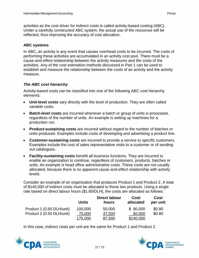
Consider an example of an organization that produces Product 1 and Product 2. A total of $140,000 of indirect costs must be allocated to these two products. Using a single rate based on direct labour hours ($1.60/DLH), the costs are allocated as follows:
Units
Direct labour hours
Cost allocated
Cost per unit
Product 1 (0.50 DLH/unit) 100,000 50,000 $ 80,000 $0.80
Product 2 (0.50 DLH/unit) 75,000 37,500 60,000 $0.80
175,000 87,500 $140,000
In this case, indirect costs per unit are the same for Product 1 and Product 2.
Intermediate Management Accounting Primer
28 / 73
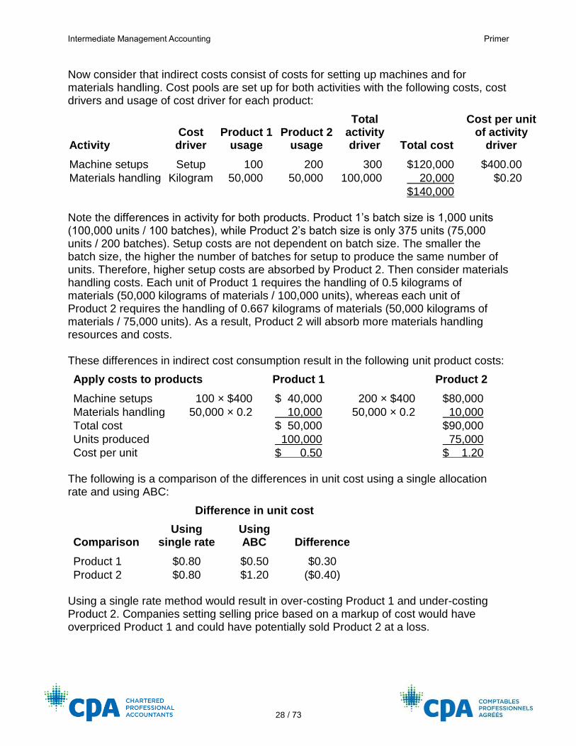
Now consider that indirect costs consist of costs for setting up machines and for materials handling. Cost pools are set up for both activities with the following costs, cost drivers and usage of cost driver for each product:
Activity Cost
driver Product 1
usage Product 2
usage
Total activity driver Total cost
Cost per unit of activity
driver
Machine setups Setup 100 200 300 $120,000 $400.00
Materials handling Kilogram 50,000 50,000 100,000 20,000 $0.20
$140,000 Note the differences in activity for both products. Product 1’s batch size is 1,000 units (100,000 units / 100 batches), while Product 2’s batch size is only 375 units (75,000 units / 200 batches). Setup costs are not dependent on batch size. The smaller the batch size, the higher the number of batches for setup to produce the same number of units. Therefore, higher setup costs are absorbed by Product 2. Then consider materials handling costs. Each unit of Product 1 requires the handling of 0.5 kilograms of materials (50,000 kilograms of materials / 100,000 units), whereas each unit of Product 2 requires the handling of 0.667 kilograms of materials (50,000 kilograms of materials / 75,000 units). As a result, Product 2 will absorb more materials handling resources and costs. These differences in indirect cost consumption result in the following unit product costs:
Apply costs to products Product 1
Product 2
Machine setups 100 × $400 $ 40,000 200 × $400 $80,000
Materials handling 50,000 × 0.2 10,000 50,000 × 0.2 10,000
Total cost $ 50,000 $90,000
Units produced 100,000 75,000
Cost per unit $ 0.50 $ 1.20 The following is a comparison of the differences in unit cost using a single allocation rate and using ABC:
Difference in unit cost
Comparison Using
single rate Using ABC Difference
Product 1 $0.80 $0.50 $0.30
Product 2 $0.80 $1.20 ($0.40) Using a single rate method would result in over-costing Product 1 and under-costing Product 2. Companies setting selling price based on a markup of cost would have overpriced Product 1 and could have potentially sold Product 2 at a loss.
Intermediate Management Accounting Primer
29 / 73
Practice questions
1. Multiple-choice questions:
i. Which of the following best describes the calculation of equivalent units for a period?
a) The number of units actually finished for the period b) The number of units that the direct materials and/or conversion expended
would have completed to 100% c) The number of units actually finished plus the unfinished units in WIP at the
end of the period d) The number of units started in the period less the unfinished units in WIP at
the end of the period Solution Option b) is correct. Equivalent units represent the efforts and resources to start and complete a unit. Thus, the time and resources put into two units that are 50% complete represent the time and resources to start and complete one unit (2 × 50% = 100%). Option a) is incorrect. This only covers the units of the finished products. Partially completed units should be converted into equivalent units based on the amount of work that has been done. Option c) is incorrect. This describes the physical units of the finished units and the units in WIP. Partially completed units should be converted into equivalent units based on the amount of work that has been done. Option d) is incorrect. This calculates the physical units started and finished.
ii. Using ABC, how would the costs of inspecting the quality of the product be accounted for?
a) As an organization-sustaining activity b) As a product-level activity c) As a batch-level activity d) As a unit-level activity
Intermediate Management Accounting Primer
30 / 73
Solution Option c) is correct. A batch-level cost is incurred whenever a batch or group of units is processed. The cost of inspecting is the same. A batch of product is inspected before being moved forward to the next step in the process. Option a) is incorrect. An organization-sustaining activity, such as general administration costs, supports the entire organization. Inspection of product quality supports activities at a lower level. Option b) is incorrect. A product-level activity, such as design, supports individual products or services regardless of the number of units or batches produced. Therefore, it is not limited to one batch, whereas inspecting a batch of products for quality would be. Option d) is incorrect. Inspection is done on a number of units, but the cost is not driven by the unit. The cost is driven by the number of batches, not by the number of units in the batch.
2. Clyde’s Cleaning Supplies makes a liquid industrial cleaner for the shipbuilding industry. The ingredients for the liquid cleaner pass through the Mixing department and the Finishing department, where the cleaner is put into containers. The information for the Mixing department for March is as follows:
Beginning WIP 4,000 litres
Units started 18,000 litres
Units completed 19,000 litres
Beginning WIP direct ingredients $7,400
Beginning WIP conversion $1,200
Direct ingredients added during the month $33,300
Conversion costs added during the month $30,832
The company uses the weighted average method of process costing. Beginning WIP was 20% complete as to conversion. Direct ingredients are added at the beginning of the process. All conversion costs are incurred evenly throughout the process. Ending WIP was 60% complete. Before the cost accountant had a chance to prepare the production report, the company president added up all of the costs for the month and divided by the units transferred. This resulted in a unit cost of $3.828 for the month. The president is concerned about rising costs because the original budget for the month was a unit cost of $3.40.
Intermediate Management Accounting Primer
31 / 73
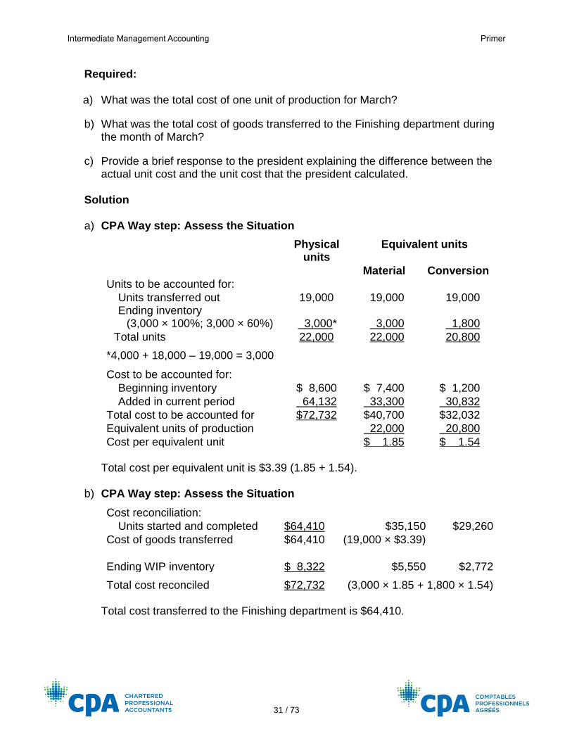
Required: a) What was the total cost of one unit of production for March?
b) What was the total cost of goods transferred to the Finishing department during the month of March?
c) Provide a brief response to the president explaining the difference between the actual unit cost and the unit cost that the president calculated.
Solution a) CPA Way step: Assess the Situation
Physical
units Equivalent units
Material Conversion
Units to be accounted for: Units transferred out 19,000 19,000 19,000 Ending inventory
(3,000 × 100%; 3,000 × 60%) 3,000* 3,000 1,800
Total units 22,000 22,000 20,800
*4,000 + 18,000 – 19,000 = 3,000
Cost to be accounted for: Beginning inventory $ 8,600 $ 7,400 $ 1,200
Added in current period 64,132 33,300 30,832
Total cost to be accounted for $72,732 $40,700 $32,032
Equivalent units of production 22,000 20,800
Cost per equivalent unit $ 1.85 $ 1.54 Total cost per equivalent unit is $3.39 (1.85 + 1.54).
b) CPA Way step: Assess the Situation
Cost reconciliation: Units started and completed $64,410 $35,150 $29,260
Cost of goods transferred $64,410 (19,000 × $3.39)
Ending WIP inventory $ 8,322 $5,550 $2,772
Total cost reconciled $72,732 (3,000 × 1.85 + 1,800 × 1.54) Total cost transferred to the Finishing department is $64,410.
Intermediate Management Accounting Primer
32 / 73
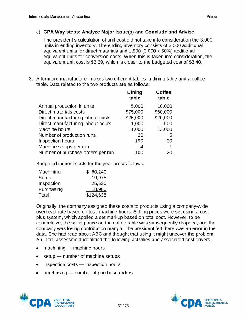
c) CPA Way steps: Analyze Major Issue(s) and Conclude and Advise
The president’s calculation of unit cost did not take into consideration the 3,000 units in ending inventory. The ending inventory consists of 3,000 additional equivalent units for direct materials and 1,800 (3,000 × 60%) additional equivalent units for conversion costs. When this is taken into consideration, the equivalent unit cost is $3.39, which is closer to the budgeted cost of $3.40.
3. A furniture manufacturer makes two different tables: a dining table and a coffee table. Data related to the two products are as follows:
Dining table
Coffee table
Annual production in units 5,000 10,000
Direct materials costs $75,000 $60,000
Direct manufacturing labour costs $25,000 $20,000
Direct manufacturing labour hours 1,000 500
Machine hours 11,000 13,000
Number of production runs 20 5
Inspection hours 190 30
Machine setups per run 4 1
Number of purchase orders per run 100 20 Budgeted indirect costs for the year are as follows:
Machining $ 60,240
Setup 19,975
Inspection 25,520
Purchasing 18,900
Total $124,635 Originally, the company assigned these costs to products using a company-wide overhead rate based on total machine hours. Selling prices were set using a cost-plus system, which applied a set markup based on total cost. However, to be competitive, the selling price on the coffee table was subsequently dropped, and the company was losing contribution margin. The president felt there was an error in the data. She had read about ABC and thought that using it might uncover the problem. An initial assessment identified the following activities and associated cost drivers:
• machining — machine hours
• setup — number of machine setups
• inspection costs — inspection hours
• purchasing — number of purchase orders
Intermediate Management Accounting Primer
33 / 73
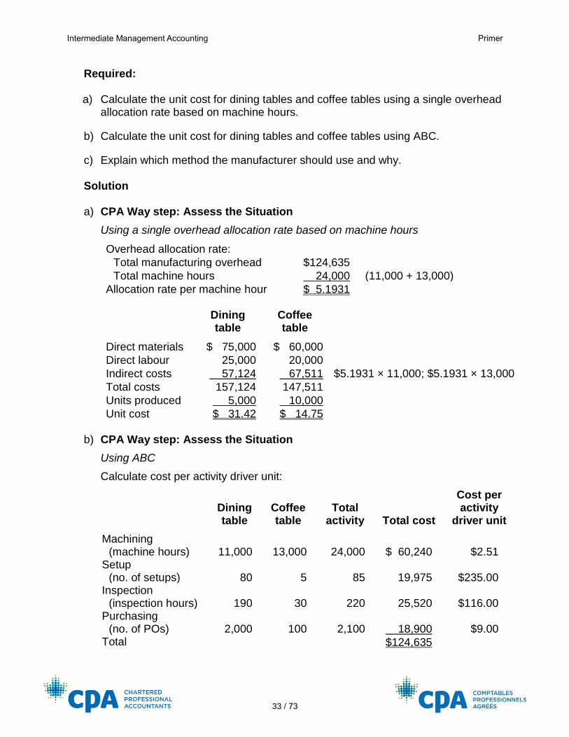
Required: a) Calculate the unit cost for dining tables and coffee tables using a single overhead
allocation rate based on machine hours.
b) Calculate the unit cost for dining tables and coffee tables using ABC.
c) Explain which method the manufacturer should use and why. Solution a) CPA Way step: Assess the Situation
Using a single overhead allocation rate based on machine hours
Overhead allocation rate: Total manufacturing overhead $124,635 Total machine hours 24,000 (11,000 + 13,000)
Allocation rate per machine hour $ 5.1931
Dining table
Coffee table
Direct materials $ 75,000 $ 60,000 Direct labour 25,000 20,000 Indirect costs 57,124 67,511 $5.1931 × 11,000; $5.1931 × 13,000
Total costs 157,124 147,511 Units produced 5,000 10,000 Unit cost $ 31.42 $ 14.75
b) CPA Way step: Assess the Situation
Using ABC
Calculate cost per activity driver unit:
Dining table
Coffee table
Total activity Total cost
Cost per activity
driver unit
Machining (machine hours) 11,000 13,000 24,000 $ 60,240 $2.51
Setup (no. of setups) 80 5 85 19,975 $235.00
Inspection (inspection hours) 190 30 220 25,520 $116.00
Purchasing (no. of POs) 2,000 100 2,100 18,900 $9.00
Total $124,635
Intermediate Management Accounting Primer
34 / 73
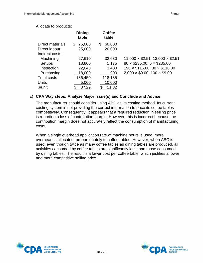
Allocate to products:
Dining table
Coffee table
Direct materials $ 75,000 $ 60,000 Direct labour 25,000 20,000 Indirect costs:
Machining 27,610 32,630 11,000 × $2.51; 13,000 × $2.51
Setups 18,800 1,175 80 × $235.00; 5 × $235.00
Inspection 22,040 3,480 190 × $116.00; 30 × $116.00
Purchasing 18,000 900 2,000 × $9.00; 100 × $9.00
Total costs 186,450 118,185 Units 5,000 10,000 $/unit $ 37.29 $ 11.82
c) CPA Way steps: Analyze Major Issue(s) and Conclude and Advise
The manufacturer should consider using ABC as its costing method. Its current costing system is not providing the correct information to price its coffee tables competitively. Consequently, it appears that a required reduction in selling price is reporting a loss of contribution margin. However, this is incorrect because the contribution margin does not accurately reflect the consumption of manufacturing costs. When a single overhead application rate of machine hours is used, more overhead is allocated, proportionately to coffee tables. However, when ABC is used, even though twice as many coffee tables as dining tables are produced, all activities consumed by coffee tables are significantly less than those consumed by dining tables. The result is a lower cost per coffee table, which justifies a lower and more competitive selling price.
Intermediate Management Accounting Primer
35 / 73
PART 4: VARIOUS COSTING METHODS AND BUDGETING
Variable (direct), absorption (full) and throughput costing
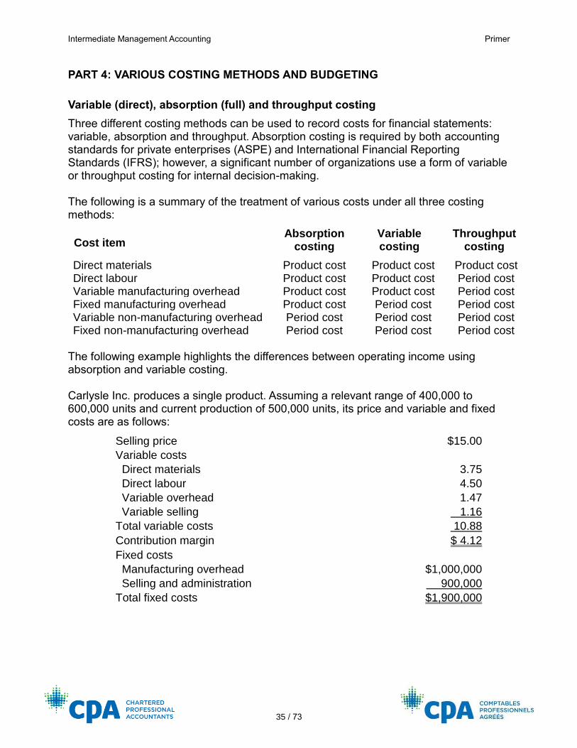
Three different costing methods can be used to record costs for financial statements: variable, absorption and throughput. Absorption costing is required by both accounting standards for private enterprises (ASPE) and International Financial Reporting Standards (IFRS); however, a significant number of organizations use a form of variable or throughput costing for internal decision-making. The following is a summary of the treatment of various costs under all three costing methods:
Cost item Absorption
costing Variable costing
Throughput costing
Direct materials Product cost Product cost Product cost Direct labour Product cost Product cost Period cost Variable manufacturing overhead Product cost Product cost Period cost Fixed manufacturing overhead Product cost Period cost Period cost Variable non-manufacturing overhead Period cost Period cost Period cost Fixed non-manufacturing overhead Period cost Period cost Period cost
The following example highlights the differences between operating income using absorption and variable costing. Carlysle Inc. produces a single product. Assuming a relevant range of 400,000 to 600,000 units and current production of 500,000 units, its price and variable and fixed costs are as follows:
Selling price $15.00
Variable costs
Direct materials 3.75
Direct labour 4.50
Variable overhead 1.47
Variable selling 1.16
Total variable costs 10.88
Contribution margin $ 4.12
Fixed costs
Manufacturing overhead $1,000,000
Selling and administration 900,000
Total fixed costs $1,900,000
Intermediate Management Accounting Primer
36 / 73
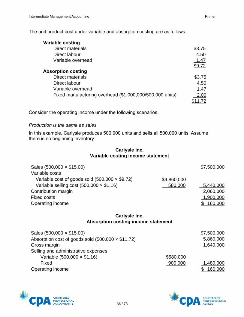
The unit product cost under variable and absorption costing are as follows:
Variable costing
Direct materials $3.75
Direct labour 4.50
Variable overhead 1.47 $9.72
Absorption costing
Direct materials $3.75
Direct labour 4.50
Variable overhead 1.47
Fixed manufacturing overhead ($1,000,000/500,000 units) 2.00
$11.72
Consider the operating income under the following scenarios.
Production is the same as sales
In this example, Carlysle produces 500,000 units and sells all 500,000 units. Assume there is no beginning inventory.
Carlysle Inc.
Variable costing income statement
Sales (500,000 × $15.00) $7,500,000
Variable costs
Variable cost of goods sold (500,000 × $9.72) $4,860,000 Variable selling cost (500,000 × $1.16) 580,000 5,440,000
Contribution margin 2,060,000
Fixed costs 1,900,000
Operating income $ 160,000
Carlysle Inc.
Absorption costing income statement
Sales (500,000 × $15.00) $7,500,000
Absorption cost of goods sold (500,000 × $11.72) 5,860,000
Gross margin 1,640,000
Selling and administrative expenses
Variable (500,000 × $1.16) $580,000
Fixed 900,000 1,480,000
Operating income $ 160,000
Intermediate Management Accounting Primer
37 / 73
Note that the variable costing income statement only considers variable manufacturing costs as product costs. Fixed manufacturing overhead is expensed in the period incurred, making it a period cost. In contrast, absorption costing considers all manufacturing costs to be product costs. As such, fixed manufacturing costs of unsold inventory are carried as an asset in the inventory account until the product is sold. In this example, because all inventory produced is sold, there is no difference in operating income between both options.
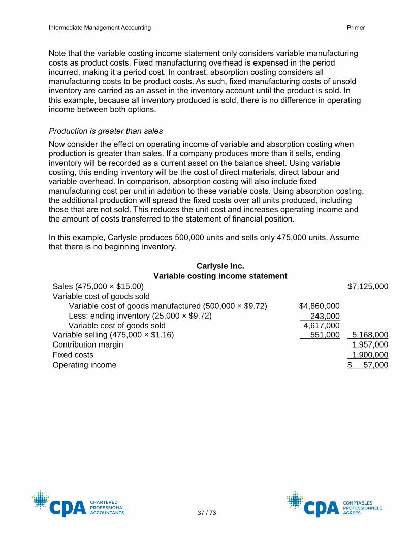
Production is greater than sales
Now consider the effect on operating income of variable and absorption costing when production is greater than sales. If a company produces more than it sells, ending inventory will be recorded as a current asset on the balance sheet. Using variable costing, this ending inventory will be the cost of direct materials, direct labour and variable overhead. In comparison, absorption costing will also include fixed manufacturing cost per unit in addition to these variable costs. Using absorption costing, the additional production will spread the fixed costs over all units produced, including those that are not sold. This reduces the unit cost and increases operating income and the amount of costs transferred to the statement of financial position. In this example, Carlysle produces 500,000 units and sells only 475,000 units. Assume that there is no beginning inventory.
Carlysle Inc.
Variable costing income statement
Sales (475,000 × $15.00)
$7,125,000
Variable cost of goods sold
Variable cost of goods manufactured (500,000 × $9.72) $4,860,000
Less: ending inventory (25,000 × $9.72) 243,000
Variable cost of goods sold 4,617,000
Variable selling (475,000 × $1.16) 551,000 5,168,000
Contribution margin
1,957,000
Fixed costs 1,900,000
Operating income $ 57,000
Intermediate Management Accounting Primer
38 / 73
Carlysle Inc.
Absorption costing income statement
Sales (475,000 × $15.00)
$7,125,000
Cost of goods sold
Absorption cost of goods manufactured (500,000 × $11.72) $5,860,000
Less: ending inventory (25,000 × $11.72) 293,000
Cost of goods sold 5,567,000
Gross margin
1,558,000
Selling and administrative expenses
Variable selling (475,000 × $1.16) 551,000
Fixed 900,000 1,451,000
Operating income
$ 107,000
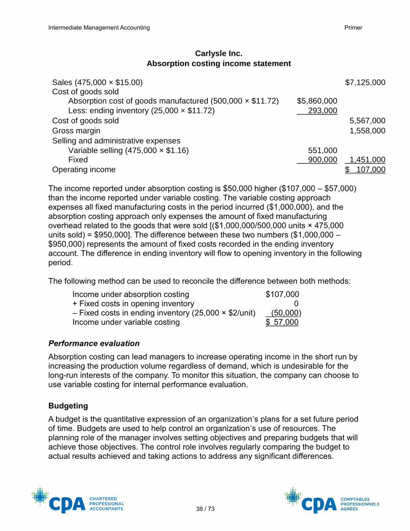
The income reported under absorption costing is $50,000 higher ($107,000 – $57,000) than the income reported under variable costing. The variable costing approach expenses all fixed manufacturing costs in the period incurred ($1,000,000), and the absorption costing approach only expenses the amount of fixed manufacturing overhead related to the goods that were sold [($1,000,000/500,000 units × 475,000 units sold) = $950,000]. The difference between these two numbers ($1,000,000 – $950,000) represents the amount of fixed costs recorded in the ending inventory account. The difference in ending inventory will flow to opening inventory in the following period. The following method can be used to reconcile the difference between both methods:
Income under absorption costing $107,000 + Fixed costs in opening inventory 0 – Fixed costs in ending inventory (25,000 × $2/unit) (50,000) Income under variable costing $ 57,000
Performance evaluation
Absorption costing can lead managers to increase operating income in the short run by increasing the production volume regardless of demand, which is undesirable for the long-run interests of the company. To monitor this situation, the company can choose to use variable costing for internal performance evaluation.
Budgeting
A budget is the quantitative expression of an organization’s plans for a set future period of time. Budgets are used to help control an organization’s use of resources. The planning role of the manager involves setting objectives and preparing budgets that will achieve those objectives. The control role involves regularly comparing the budget to actual results achieved and taking actions to address any significant differences.
Intermediate Management Accounting Primer
39 / 73
The budget is usually prepared by a budget committee consisting of managers who control the costs and revenues of the organization. An operating budget is prepared for the company’s fiscal year, and a capital budget can span several years.
The master budget
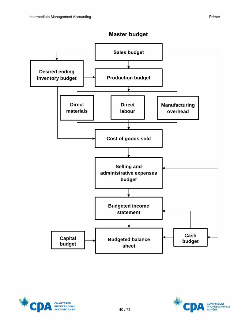
The master budget is the overall budget plan. It begins with the organization’s business strategies and sales forecasts. The organization’s objectives result in a formal sales budget that identifies the planned level of sales for the organization’s products. The sales budget, combined with the organization’s inventory policy, results in the production plan for a manufacturing company and a purchase plan for a merchandising company.
For manufacturing companies, details of the production plan trigger the activities needed to support production. These activity triggers may include the need to acquire additional machinery or to hire or lay off employees and the amount and timing of raw materials for production. The sales budget can also be used to estimate selling and administration expenses to complete the budgeted income statement. Cash collections estimated based on the sales budget, together with cash disbursements, will be used to develop the cash budget and the balance in accounts receivable/payable for the statement of financial position. The following diagram summarizes the components and interrelationships of the master budget components for a manufacturing company.
Intermediate Management Accounting Primer
40 / 73
Sales budget
Production budget
Direct
materials
Direct
labour
Desired ending
inventory budget
Cost of goods sold
Selling and
administrative expenses
budget
Budgeted income
statement
Budgeted balance
sheet
Cash budget
Capital budget
Master budget
Manufacturing
overhead
Intermediate Management Accounting Primer
41 / 73
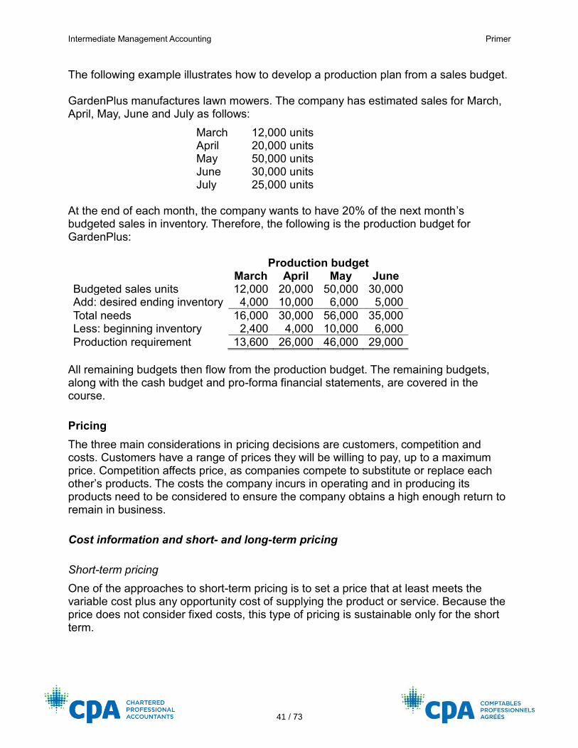
The following example illustrates how to develop a production plan from a sales budget. GardenPlus manufactures lawn mowers. The company has estimated sales for March, April, May, June and July as follows:
March 12,000 units April 20,000 units May 50,000 units June 30,000 units July 25,000 units
At the end of each month, the company wants to have 20% of the next month’s budgeted sales in inventory. Therefore, the following is the production budget for GardenPlus: Production budget March April May June Budgeted sales units 12,000 20,000 50,000 30,000 Add: desired ending inventory 4,000 10,000 6,000 5,000
Total needs 16,000 30,000 56,000 35,000 Less: beginning inventory 2,400 4,000 10,000 6,000
Production requirement 13,600 26,000 46,000 29,000
All remaining budgets then flow from the production budget. The remaining budgets, along with the cash budget and pro-forma financial statements, are covered in the course.
Pricing
The three main considerations in pricing decisions are customers, competition and costs. Customers have a range of prices they will be willing to pay, up to a maximum price. Competition affects price, as companies compete to substitute or replace each other’s products. The costs the company incurs in operating and in producing its products need to be considered to ensure the company obtains a high enough return to remain in business.
Cost information and short- and long-term pricing
Short-term pricing
One of the approaches to short-term pricing is to set a price that at least meets the variable cost plus any opportunity cost of supplying the product or service. Because the price does not consider fixed costs, this type of pricing is sustainable only for the short term.

Intermediate Management Accounting Primer
42 / 73
Long-term pricing
The three main choices for long-term pricing are market pricing, cost-based pricing and cost-plus pricing. Market pricing is used in a competitive environment; a business examines the market and its customers to determine what the market will pay for its product. In cost-based pricing, a business factors in fixed costs as well as variable costs when setting a long-term price for a product. The most widely used approach is cost-plus pricing, whereby a markup is added to the cost base. This approach reflects a stable, long-term equilibrium price that supports both demand and supply. The following example illustrates how a selling price is set using the estimated costs of a product over its lifetime. TubZone is developing a new solar-powered hot tub called the SolarSpa. The company predicts that customers will be willing to pay a higher price for this product because the solar cells used to heat the tub will produce constant, even heat in areas that receive little direct sunlight. Marketing expects to sell an average of 2,500 SolarSpa tubs per year and expects demand to last for eight years. To appropriately price this product, the cost accountant worked with the development team to arrive at the following prospective costs. TubZone marks up its products by 30% of the lifetime costs to provide a satisfactory return on investment.
SolarSpa — Lifetime costs Per unit Annual
(2,500 units)
Total for product life
(8 years)
Unit costs
Direct materials cost $1,300
Direct labour cost 840
Variable manufacturing overhead cost 960
Variable selling, general and administrative costs 500
Total variable costs $3,600 $9,000,000 $ 72,000,000
Annual costs
Fixed manufacturing 2,500,000 20,000,000
Fixed selling, general and administrative 450,000 3,600,000
Cost of quality 160,000 1,280,000
One-time costs
Product development costs 10,000,000
Product abandonment costs 1,520,000
Total product-related costs $108,400,000
Total lifetime unit sales (2,500 × 8 years) 20,000
Total product cost per unit $ 5,420
Prospective selling price (30% markup) $ 7,046
Other factors should be considered when using cost-based prices. Prices are subject to factors such as fluctuating demand and competition. Some companies, such as airlines,
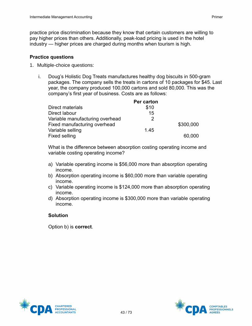
Intermediate Management Accounting Primer
43 / 73
practice price discrimination because they know that certain customers are willing to pay higher prices than others. Additionally, peak-load pricing is used in the hotel industry — higher prices are charged during months when tourism is high.
Practice questions
1. Multiple-choice questions: i. Doug’s Holistic Dog Treats manufactures healthy dog biscuits in 500-gram
packages. The company sells the treats in cartons of 10 packages for $45. Last year, the company produced 100,000 cartons and sold 80,000. This was the company’s first year of business. Costs are as follows:
Per carton Direct materials $10 Direct labour 15 Variable manufacturing overhead 2 Fixed manufacturing overhead $300,000 Variable selling 1.45 Fixed selling 60,000 What is the difference between absorption costing operating income and variable costing operating income? a) Variable operating income is $56,000 more than absorption operating
income. b) Absorption operating income is $60,000 more than variable operating
income. c) Variable operating income is $124,000 more than absorption operating
income. d) Absorption operating income is $300,000 more than variable operating
income. Solution Option b) is correct.
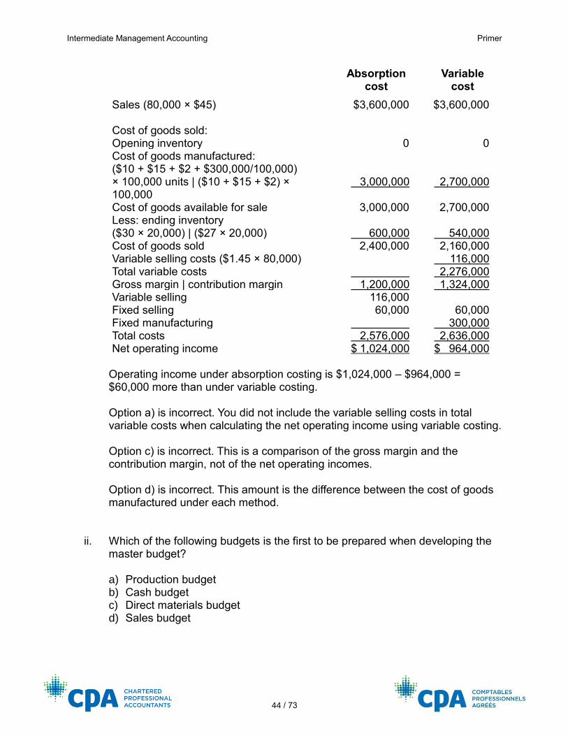
Intermediate Management Accounting Primer
44 / 73
Absorption cost
Variable cost
Sales (80,000 × $45) $3,600,000 $3,600,000 Cost of goods sold: Opening inventory 0 0 Cost of goods manufactured: ($10 + $15 + $2 + $300,000/100,000) × 100,000 units | ($10 + $15 + $2) × 100,000
3,000,000
2,700,000
Cost of goods available for sale 3,000,000 2,700,000 Less: ending inventory ($30 × 20,000) | ($27 × 20,000)
600,000
540,000
Cost of goods sold 2,400,000 2,160,000 Variable selling costs ($1.45 × 80,000) 116,000 Total variable costs 2,276,000 Gross margin | contribution margin 1,200,000 1,324,000 Variable selling 116,000 Fixed selling 60,000 60,000 Fixed manufacturing 300,000 Total costs 2,576,000 2,636,000 Net operating income $ 1,024,000 $ 964,000
Operating income under absorption costing is $1,024,000 – $964,000 = $60,000 more than under variable costing. Option a) is incorrect. You did not include the variable selling costs in total variable costs when calculating the net operating income using variable costing. Option c) is incorrect. This is a comparison of the gross margin and the contribution margin, not of the net operating incomes. Option d) is incorrect. This amount is the difference between the cost of goods manufactured under each method.
ii. Which of the following budgets is the first to be prepared when developing the master budget?
a) Production budget b) Cash budget c) Direct materials budget d) Sales budget
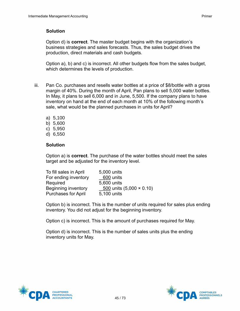
Intermediate Management Accounting Primer
45 / 73
Solution Option d) is correct. The master budget begins with the organization’s business strategies and sales forecasts. Thus, the sales budget drives the production, direct materials and cash budgets. Option a), b) and c) is incorrect. All other budgets flow from the sales budget, which determines the levels of production.
iii. Pan Co. purchases and resells water bottles at a price of $8/bottle with a gross margin of 40%. During the month of April, Pan plans to sell 5,000 water bottles. In May, it plans to sell 6,000 and in June, 5,500. If the company plans to have inventory on hand at the end of each month at 10% of the following month’s sale, what would be the planned purchases in units for April?
a) 5,100 b) 5,600 c) 5,950 d) 6,550
Solution
Option a) is correct. The purchase of the water bottles should meet the sales target and be adjusted for the inventory level. To fill sales in April 5,000 units For ending inventory 600 units Required 5,600 units Beginning inventory 500 units (5,000 × 0.10) Purchases for April 5,100 units Option b) is incorrect. This is the number of units required for sales plus ending inventory. You did not adjust for the beginning inventory. Option c) is incorrect. This is the amount of purchases required for May. Option d) is incorrect. This is the number of sales units plus the ending inventory units for May.
Intermediate Management Accounting Primer
46 / 73
2. Alarums Ltd. produces Wi-Fi home security alarms. The company had the following results for January 20X1:.
Units: January
Beginning inventory 0
Production 1,000
Sales 900
Ending inventory 100
Costs:
Variable manufacturing costs per unit:
Direct materials $10
Direct labour 5
Variable manufacturing overhead 3
Variable marketing costs per unit 2
Fixed manufacturing overhead 8,000
Fixed marketing and administrative costs 12,000
Sales price per unit $45
The president has heard that there are alternatives to the inventory costing and wonders if management control might be better using an alternative. Required: Analyze and recommend to management which method of costing (absorption or variable) to use for management control purposes.
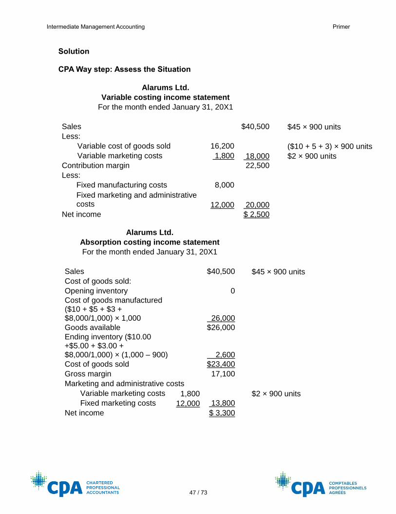
Intermediate Management Accounting Primer
47 / 73
Solution
CPA Way step: Assess the Situation
Alarums Ltd. Variable costing income statement
For the month ended January 31, 20X1
Sales $40,500 $45 × 900 units
Less: Variable cost of goods sold 16,200 ($10 + 5 + 3) × 900 units
Variable marketing costs 1,800 18,000 $2 × 900 units
Contribution margin 22,500 Less:
Fixed manufacturing costs 8,000 Fixed marketing and administrative costs 12,000 20,000
Net income $ 2,500
Alarums Ltd.
Absorption costing income statement
For the month ended January 31, 20X1
Sales $40,500 $45 × 900 units
Cost of goods sold:
Opening inventory 0 Cost of goods manufactured ($10 + $5 + $3 + $8,000/1,000) × 1,000 26,000
Goods available $26,000 Ending inventory ($10.00 +$5.00 + $3.00 + $8,000/1,000) × (1,000 – 900) 2,600
Cost of goods sold $23,400
Gross margin 17,100
Marketing and administrative costs
Variable marketing costs 1,800 $2 × 900 units
Fixed marketing costs 12,000 13,800
Net income $ 3,300
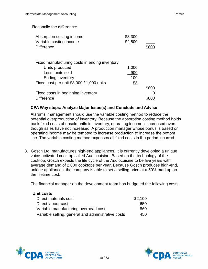
Intermediate Management Accounting Primer
48 / 73
Reconcile the difference:
Absorption costing income $3,300 Variable costing income $2,500
Difference $800
Fixed manufacturing costs in ending inventory
Units produced 1,000 Less: units sold 900 Ending inventory 100
Fixed cost per unit $8,000 / 1,000 units $8
$800
Fixed costs in beginning inventory 0
Difference $800
CPA Way steps: Analyze Major Issue(s) and Conclude and Advise
Alarums’ management should use the variable costing method to reduce the potential overproduction of inventory. Because the absorption costing method holds back fixed costs of unsold units in inventory, operating income is increased even though sales have not increased. A production manager whose bonus is based on operating income may be tempted to increase production to increase the bottom line. The variable costing method expenses all fixed costs in the period incurred.
3. .Gosch Ltd. manufactures high-end appliances. It is currently developing a unique voice-activated cooktop called Audiocuisine. Based on the technology of the cooktop, Gosch expects the life cycle of the Audiocuisine to be five years with average demand of 2,000 cooktops per year. Because Gosch produces high-end, unique appliances, the company is able to set a selling price at a 50% markup on the lifetime cost. The financial manager on the development team has budgeted the following costs:
Unit costs
Direct materials cost $2,100
Direct labour cost 650
Variable manufacturing overhead cost 860
Variable selling, general and administrative costs 450
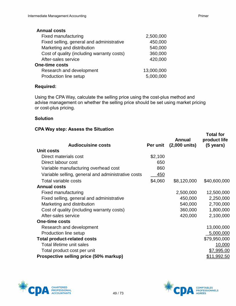
Intermediate Management Accounting Primer
49 / 73
Annual costs
Fixed manufacturing 2,500,000
Fixed selling, general and administrative 450,000
Marketing and distribution 540,000
Cost of quality (including warranty costs) 360,000
After-sales service 420,000
One-time costs
Research and development 13,000,000
Production line setup 5,000,000
Required: Using the CPA Way, calculate the selling price using the cost-plus method and advise management on whether the selling price should be set using market pricing or cost-plus pricing. Solution
CPA Way step: Assess the Situation
Audiocuisine costs Per unit Annual
(2,000 units)
Total for product life
(5 years)
Unit costs
Direct materials cost $2,100
Direct labour cost 650
Variable manufacturing overhead cost 860
Variable selling, general and administrative costs 450
Total variable costs $4,060 $8,120,000 $40,600,000
Annual costs
Fixed manufacturing 2,500,000 12,500,000
Fixed selling, general and administrative 450,000 2,250,000
Marketing and distribution 540,000 2,700,000
Cost of quality (including warranty costs) 360,000 1,800,000
After-sales service 420,000 2,100,000
One-time costs
Research and development 13,000,000
Production line setup 5,000,000
Total product-related costs $79,950,000
Total lifetime unit sales 10,000
Total product cost per unit $ 7,995.00
Prospective selling price (50% markup) $11,992.50
Intermediate Management Accounting Primer
50 / 73
CPA Way steps: Analyze Major Issue(s) and Conclude and Advise
The Audiocuisine is a unique product with little competition in the market. As such, customers would be willing to pay a higher price for the product, and there is less concern over costs. Market-based pricing is used in a competitive environment where sales are based on a price that is better than the competition. In this situation, management should set the price using cost-plus pricing.
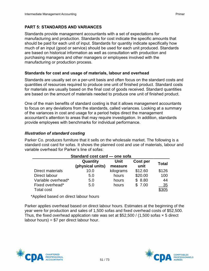
Intermediate Management Accounting Primer
51 / 73
PART 5: STANDARDS AND VARIANCES
Standards provide management accountants with a set of expectations for manufacturing and production. Standards for cost indicate the specific amounts that should be paid for each unit of input. Standards for quantity indicate specifically how much of an input (good or service) should be used for each unit produced. Standards are based on historical information as well as consultation with production and purchasing managers and other managers or employees involved with the manufacturing or production process.
Standards for cost and usage of materials, labour and overhead
Standards are usually set on a per-unit basis and often focus on the standard costs and quantities of resources required to produce one unit of finished product. Standard costs for materials are usually based on the final cost of goods received. Standard quantities are based on the amount of materials needed to produce one unit of finished product. One of the main benefits of standard costing is that it allows management accountants to focus on any deviations from the standards, called variances. Looking at a summary of the variances in cost and usage for a period helps direct the management accountant’s attention to areas that may require investigation. In addition, standards provide employees with benchmarks for individual performance.
Illustration of standard costing
Parker Co. produces furniture that it sells on the wholesale market. The following is a standard cost card for sofas. It shows the planned cost and use of materials, labour and variable overhead for Parker’s line of sofas:
Standard cost card — one sofa
Quantity (physical units)
Unit measure
Cost per unit
Total
Direct materials 10.0 kilograms $12.60 $126 Direct labour 5.0 hours $20.00 100 Variable overhead* 5.0 hours $ 8.80 44 Fixed overhead* 5.0 hours $ 7.00 35 Total cost $305
*Applied based on direct labour hours Parker applies overhead based on direct labour hours. Estimates at the beginning of the year were for production and sales of 1,500 sofas and fixed overhead costs of $52,500. Thus, the fixed overhead application rate was set at $52,500 / (1,500 sofas × 5 direct labour hours) = $7 per direct labour hour.
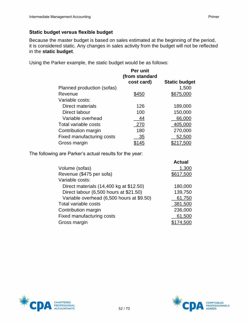
Intermediate Management Accounting Primer
52 / 73
Static budget versus flexible budget
Because the master budget is based on sales estimated at the beginning of the period, it is considered static. Any changes in sales activity from the budget will not be reflected in the static budget. Using the Parker example, the static budget would be as follows:
Per unit (from standard
cost card) Static budget
Planned production (sofas) 1,500
Revenue $450 $675,000
Variable costs:
Direct materials 126 189,000
Direct labour 100 150,000
Variable overhead 44 66,000
Total variable costs 270 405,000
Contribution margin 180 270,000
Fixed manufacturing costs 35 52,500
Gross margin $145 $217,500
The following are Parker’s actual results for the year:
Actual
Volume (sofas) 1,300
Revenue ($475 per sofa) $617,500
Variable costs:
Direct materials (14,400 kg at $12.50) 180,000
Direct labour (6,500 hours at $21.50) 139,750
Variable overhead (6,500 hours at $9.50) 61,750
Total variable costs 381,500
Contribution margin 236,000
Fixed manufacturing costs 61,500
Gross margin $174,500
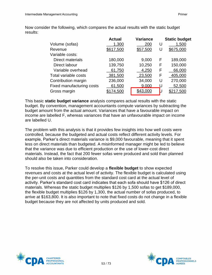
Intermediate Management Accounting Primer
53 / 73
Now consider the following, which compares the actual results with the static budget results:
Actual Variance Static budget
Volume (sofas) 1,300 200 U 1,500
Revenue $617,500 $57,500 U $675,000
Variable costs:
Direct materials 180,000 9,000 F 189,000
Direct labour 139,750 10,250 F 150,000
Variable overhead 61,750 4,250 F 66,000
Total variable costs 381,500 23,500 F 405,000
Contribution margin 236,000 34,000 U 270,000
Fixed manufacturing costs 61,500 9,000 U 52,500
Gross margin $174,500 $43,000 U $217,500
This basic static budget variance analysis compares actual results with the static budget. By convention, management accountants compute variances by subtracting the budget amount from the actual amount. Variances that have a favourable impact on income are labelled F, whereas variances that have an unfavourable impact on income are labelled U. The problem with this analysis is that it provides few insights into how well costs were controlled, because the budgeted and actual costs reflect different activity levels. For example, Parker’s direct materials variance is $9,000 favourable, meaning that it spent less on direct materials than budgeted. A misinformed manager might be led to believe that the variance was due to efficient production or the use of lower-cost direct materials. Instead, the fact that 200 fewer sofas were produced and sold than planned should also be taken into consideration.
To resolve this issue, Parker could develop a flexible budget to show expected revenues and costs at the actual level of activity. The flexible budget is calculated using the per-unit costs and quantities from the standard cost card at the actual level of activity. Parker’s standard cost card indicates that each sofa should have $126 of direct materials. Whereas the static budget multiplies $126 by 1,500 sofas to get $189,000, the flexible budget multiplies $126 by 1,300, the actual number of sofas produced, to arrive at $163,800. It is also important to note that fixed costs do not change in a flexible budget because they are not affected by units produced and sold.
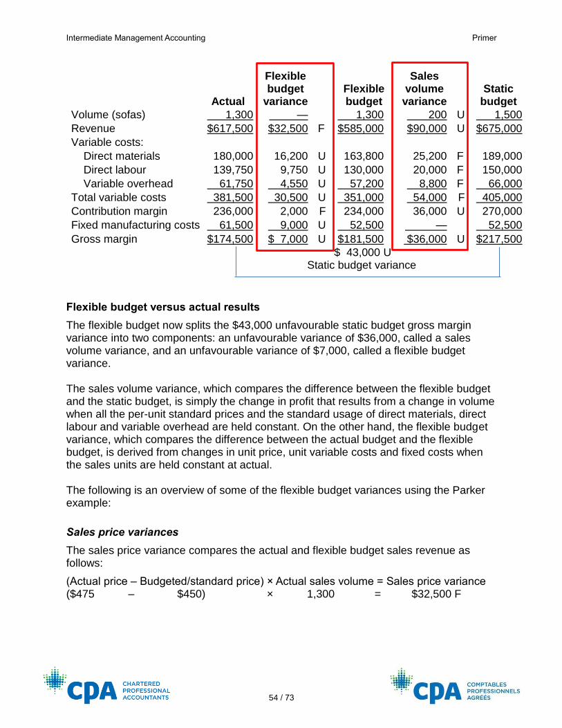
Intermediate Management Accounting Primer
54 / 73
Actual
Flexible budget
variance
Flexible budget
Sales volume
variance
Static budget
Volume (sofas) 1,300 — 1,300 200 U 1,500
Revenue $617,500 $32,500 F $585,000 $90,000 U $675,000
Variable costs:
Direct materials 180,000 16,200 U 163,800 25,200 F 189,000
Direct labour 139,750 9,750 U 130,000 20,000 F 150,000
Variable overhead 61,750 4,550 U 57,200 8,800 F 66,000
Total variable costs 381,500 30,500 U 351,000 54,000 F 405,000
Contribution margin 236,000 2,000 F 234,000 36,000 U 270,000
Fixed manufacturing costs 61,500 9,000 U 52,500 — 52,500
Gross margin $174,500 $ 7,000 U $181,500 $36,000 U $217,500
$ 43,000 U Static budget variance
Flexible budget versus actual results
The flexible budget now splits the $43,000 unfavourable static budget gross margin variance into two components: an unfavourable variance of $36,000, called a sales volume variance, and an unfavourable variance of $7,000, called a flexible budget variance. The sales volume variance, which compares the difference between the flexible budget and the static budget, is simply the change in profit that results from a change in volume when all the per-unit standard prices and the standard usage of direct materials, direct labour and variable overhead are held constant. On the other hand, the flexible budget variance, which compares the difference between the actual budget and the flexible budget, is derived from changes in unit price, unit variable costs and fixed costs when the sales units are held constant at actual. The following is an overview of some of the flexible budget variances using the Parker example:
Sales price variances
The sales price variance compares the actual and flexible budget sales revenue as follows:
(Actual price – Budgeted/standard price) × Actual sales volume = Sales price variance ($475 – $450) × 1,300 = $32,500 F
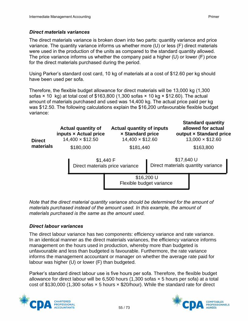
Intermediate Management Accounting Primer
55 / 73
Direct materials variances
The direct materials variance is broken down into two parts: quantity variance and price variance. The quantity variance informs us whether more (U) or less (F) direct materials were used in the production of the units as compared to the standard quantity allowed. The price variance informs us whether the company paid a higher (U) or lower (F) price for the direct materials purchased during the period. Using Parker’s standard cost card, 10 kg of materials at a cost of $12.60 per kg should have been used per sofa. Therefore, the flexible budget allowance for direct materials will be 13,000 kg (1,300 sofas × 10 kg) at total cost of $163,800 (1,300 sofas × 10 kg × $12.60). The actual amount of materials purchased and used was 14,400 kg. The actual price paid per kg was $12.50. The following calculations explain the $16,200 unfavourable flexible budget variance:
Actual quantity of
inputs × Actual price Actual quantity of inputs
× Standard price
Standard quantity allowed for actual
output × Standard price
Direct materials
14,400 × $12.50 14,400 × $12.60 13,000 × $12.60
$180,000 $181,440 $163,800
$1,440 F Direct materials price variance
$17,640 U Direct materials quantity variance
$16,200 U Flexible budget variance
Note that the direct material quantity variance should be determined for the amount of materials purchased instead of the amount used. In this example, the amount of materials purchased is the same as the amount used.
Direct labour variances
The direct labour variance has two components: efficiency variance and rate variance. In an identical manner as the direct materials variances, the efficiency variance informs management on the hours used in production, whereby more than budgeted is unfavourable and less than budgeted is favourable. Furthermore, the rate variance informs the management accountant or manager on whether the average rate paid for labour was higher (U) or lower (F) than budgeted. Parker’s standard direct labour use is five hours per sofa. Therefore, the flexible budget allowance for direct labour will be 6,500 hours (1,300 sofas × 5 hours per sofa) at a total cost of $130,000 (1,300 sofas × 5 hours × $20/hour). While the standard rate for direct
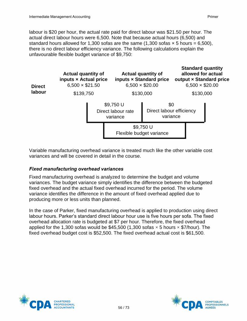
Intermediate Management Accounting Primer
56 / 73
labour is $20 per hour, the actual rate paid for direct labour was $21.50 per hour. The actual direct labour hours were 6,500. Note that because actual hours (6,500) and standard hours allowed for 1,300 sofas are the same (1,300 sofas × 5 hours = 6,500), there is no direct labour efficiency variance. The following calculations explain the unfavourable flexible budget variance of $9,750:
Actual quantity of
inputs × Actual price Actual quantity of
inputs × Standard price
Standard quantity allowed for actual
output × Standard price
Direct labour
6,500 × $21.50 6,500 × $20.00 6,500 × $20.00
$139,750 $130,000 $130,000
$9,750 U $0
Direct labour rate variance
Direct labour efficiency variance
$9,750 U
Flexible budget variance
Variable manufacturing overhead variance is treated much like the other variable cost variances and will be covered in detail in the course.
Fixed manufacturing overhead variances
Fixed manufacturing overhead is analyzed to determine the budget and volume variances. The budget variance simply identifies the difference between the budgeted fixed overhead and the actual fixed overhead incurred for the period. The volume variance identifies the difference in the amount of fixed overhead applied due to producing more or less units than planned. In the case of Parker, fixed manufacturing overhead is applied to production using direct labour hours. Parker’s standard direct labour hour use is five hours per sofa. The fixed overhead allocation rate is budgeted at $7 per hour. Therefore, the fixed overhead applied for the 1,300 sofas would be $45,500 (1,300 sofas × 5 hours × $7/hour). The fixed overhead budget cost is $52,500. The fixed overhead actual cost is $61,500.
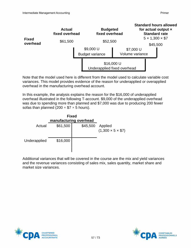
Intermediate Management Accounting Primer
57 / 73
Actual fixed overhead
Budgeted fixed overhead
Standard hours allowed for actual output ×
Standard rate
Fixed overhead
$61,500 $52,500 5 × 1,300 × $7
$45,500
$9,000 U $7,000 U
Budget variance Volume variance
$16,000 U
Underapplied fixed overhead
Note that the model used here is different from the model used to calculate variable cost variances. This model provides evidence of the reason for underapplied or overapplied overhead in the manufacturing overhead account. In this example, the analysis explains the reason for the $16,000 of underapplied overhead illustrated in the following T-account. $9,000 of the underapplied overhead was due to spending more than planned and $7,000 was due to producing 200 fewer sofas than planned (200 × $7 × 5 hours).
Fixed manufacturing overhead
Actual $61,500 $45,500 Applied
(1,300 × 5 × $7)
Underapplied $16,000
Additional variances that will be covered in the course are the mix and yield variances and the revenue variances consisting of sales mix, sales quantity, market share and market size variances.
Intermediate Management Accounting Primer
58 / 73
Practice questions
1. Multiple-choice questions: i. Balto Co. budgeted for production and sales of 63,000 units of Xeron in June,
but produced and sold only 60,000 units. Actual direct labour costs of $125,000 were incurred during this period. Direct labour cost was budgeted at $2.25 per unit. What is the flexible budget variance for the direct labour cost?
a) $10,000 F b) $10,000 U c) $16,750 F d) $16,750 U Solution Option a) is correct. At actual production, Balto planned to spend $135,000 (60,000 × $2.25). Balto actually spent $125,000. Therefore, there is a $10,000 F variance ($125,000 – $135,000). Option b) is incorrect. Balto’s actual direct labour costs are $10,000 less than the budgeted cost. This is a favourable variance. Option c) is incorrect. While this is a favourable variance, the actual cost of $125,000 was compared to the static budget cost instead of the flexible budget cost. Option d) is incorrect. The actual cost of $125,000 was compared to the static budget cost instead of the flexible budget cost. Additionally, the actual cost is less than the budgeted cost. This means that the variance would have been favourable.
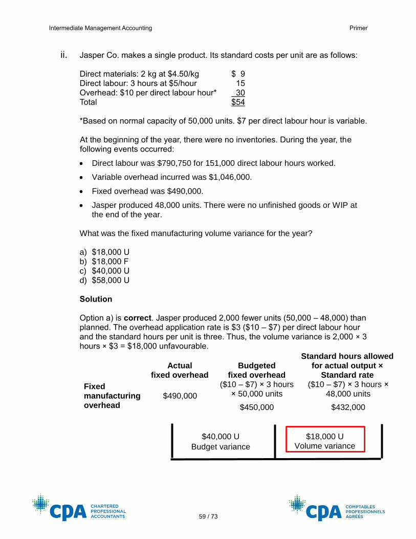
Intermediate Management Accounting Primer
59 / 73
ii. Jasper Co. makes a single product. Its standard costs per unit are as follows: Direct materials: 2 kg at $4.50/kg $ 9 Direct labour: 3 hours at $5/hour 15 Overhead: $10 per direct labour hour* 30 Total $54
*Based on normal capacity of 50,000 units. $7 per direct labour hour is variable.
At the beginning of the year, there were no inventories. During the year, the following events occurred:
• Direct labour was $790,750 for 151,000 direct labour hours worked.
• Variable overhead incurred was $1,046,000.
• Fixed overhead was $490,000.
• Jasper produced 48,000 units. There were no unfinished goods or WIP at the end of the year.
What was the fixed manufacturing volume variance for the year?
a) $18,000 U b) $18,000 F c) $40,000 U d) $58,000 U
Solution Option a) is correct. Jasper produced 2,000 fewer units (50,000 – 48,000) than planned. The overhead application rate is $3 ($10 – $7) per direct labour hour and the standard hours per unit is three. Thus, the volume variance is 2,000 × 3 hours × $3 = $18,000 unfavourable.
Actual fixed overhead
Budgeted fixed overhead
Standard hours allowed for actual output ×
Standard rate
Fixed manufacturing overhead
$490,000
($10 – $7) × 3 hours × 50,000 units
$450,000
($10 – $7) × 3 hours × 48,000 units
$432,000
$40,000 U $18,000 U
Budget variance Volume variance
Intermediate Management Accounting Primer
60 / 73
Option b) is incorrect. There is indeed an $18,000 variance; however, because Jasper produced less units than planned, it is unfavourable. Option c) is incorrect. This is the budget variance, not the volume variance. Option d) is incorrect. This is the total of the budget and volume variances, as well as the amount of underapplied overhead. This amount must be split into the budget variance and the production volume variance.
2. Valley Co. uses a standard cost system to control production costs. The following information is available for the past year:
Actual Budget Production 22,000 units 20,000 units Direct materials: Quantity 100,000 kg 5 kg per unit of output Cost $185,000 $160,000 at $1.60/kg Direct labour: Hours 10,500 hours 1 hour per unit of output Cost $160,000 $240,000 at $12/hour
There were no direct materials beginning and ending inventories for the year. Required:
a) Calculate the following:
i. Direct materials price and quantity variances
ii. Direct labour rate and efficiency variances
b) Management is concerned about the direct materials price variance. When asked, the purchasing agent informed management that the production manager wanted to purchase higher-quality, more expensive materials. Explain to management how this increase in the price of direct materials may have affected other variances.
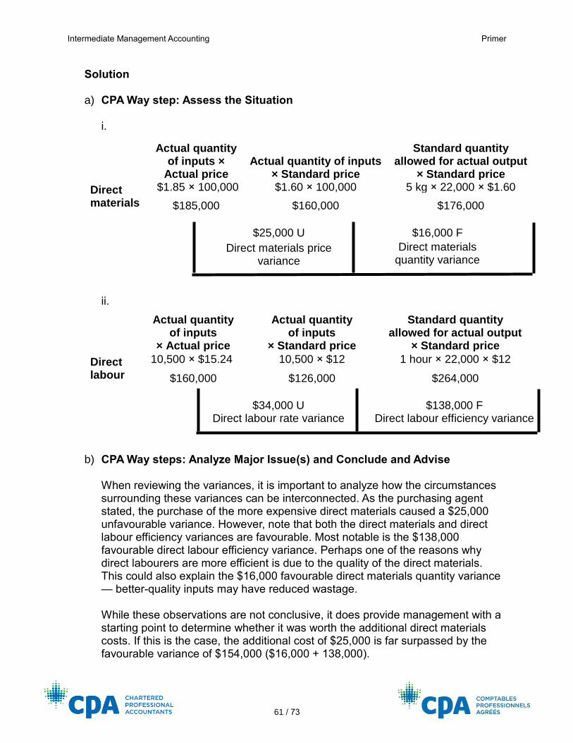
Intermediate Management Accounting Primer
61 / 73
Solution
a) CPA Way step: Assess the Situation i.
Actual quantity
of inputs × Actual price
Actual quantity of inputs × Standard price
Standard quantity allowed for actual output
× Standard price
Direct materials
$1.85 × 100,000 $1.60 × 100,000 5 kg × 22,000 × $1.60
$185,000 $160,000 $176,000
$25,000 U $16,000 F
Direct materials price variance
Direct materials quantity variance
ii.
Actual quantity
of inputs × Actual price
Actual quantity of inputs
× Standard price
Standard quantity allowed for actual output
× Standard price
Direct labour
10,500 × $15.24 10,500 × $12 1 hour × 22,000 × $12
$160,000 $126,000 $264,000
$34,000 U $138,000 F
Direct labour rate variance Direct labour efficiency variance
b) CPA Way steps: Analyze Major Issue(s) and Conclude and Advise When reviewing the variances, it is important to analyze how the circumstances surrounding these variances can be interconnected. As the purchasing agent stated, the purchase of the more expensive direct materials caused a $25,000 unfavourable variance. However, note that both the direct materials and direct labour efficiency variances are favourable. Most notable is the $138,000 favourable direct labour efficiency variance. Perhaps one of the reasons why direct labourers are more efficient is due to the quality of the direct materials. This could also explain the $16,000 favourable direct materials quantity variance — better-quality inputs may have reduced wastage. While these observations are not conclusive, it does provide management with a starting point to determine whether it was worth the additional direct materials costs. If this is the case, the additional cost of $25,000 is far surpassed by the favourable variance of $154,000 ($16,000 + 138,000).
Intermediate Management Accounting Primer
62 / 73
PART 6: RELEVANT COSTS
A relevant cost is a cost or revenue that changes as a result of a decision. The idea behind the relevant cost approach is that the decision maker need only, and should only, consider the relevant costs associated with a decision. The concept of a sunk cost is a key focus in decision-making. Sunk costs (past costs that have been incurred and are irreversible) are not relevant according to the relevant cost approach. Management accountants should ensure that sunk costs do not affect current managerial choices. When making decisions, managers must consider both quantitative and qualitative factors. Qualitative factors, such as laying off long-time, loyal personnel when eliminating a department, must be considered along with quantitative figures relating to profits and losses. Four basic relevant costing models are illustrated here; a fifth will be covered in the course.
Make-or-buy decision
Businesses often need to decide whether to produce a product (or part of a product needed in production) or purchase it from an external supplier. Relevant costs in this decision often include, but are not limited to, the costs saved from not producing the item internally, revenue that can be earned if the space is used for other purposes, and of course the cost incurred to purchase externally. Below is an example of such a decision. Calvin’s SUP Ltd. makes 30,000 stand-up paddleboards each year. One of the paddleboard components is a fin that aids the stability of the board. Currently, the fins are made by Calvin’s SUP at the following cost:
Direct materials (unit) $25.00
Direct labour (unit) $20.00
Variable manufacturing OH (unit) $4.80
Fixed manufacturing costs (total) $950,000
An outside supplier has offered to sell Calvin’s SUP all the fins it requires to manufacture its paddleboards for $58 each. If the company decides to purchase all of its fins from the outside supplier, it would lay off one plant supervisor who currently has an annual salary of $66,000. All other fixed costs relate to plant and equipment shared by all product lines and cannot be avoided.
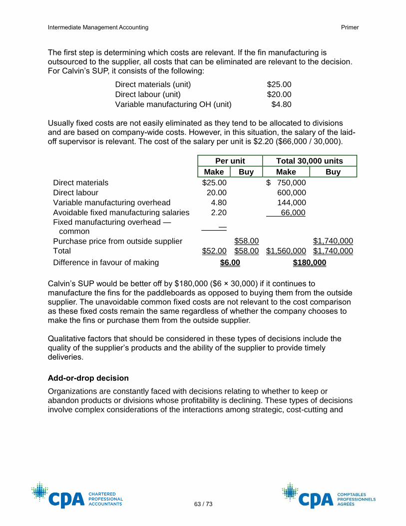
Intermediate Management Accounting Primer
63 / 73
The first step is determining which costs are relevant. If the fin manufacturing is outsourced to the supplier, all costs that can be eliminated are relevant to the decision. For Calvin’s SUP, it consists of the following:
Direct materials (unit) $25.00
Direct labour (unit) $20.00
Variable manufacturing OH (unit) $4.80
Usually fixed costs are not easily eliminated as they tend to be allocated to divisions and are based on company-wide costs. However, in this situation, the salary of the laid-off supervisor is relevant. The cost of the salary per unit is $2.20 ($66,000 / 30,000).
Per unit Total 30,000 units
Make Buy Make Buy
Direct materials $25.00 $ 750,000
Direct labour 20.00 600,000 Variable manufacturing overhead 4.80 144,000 Avoidable fixed manufacturing salaries 2.20 66,000 Fixed manufacturing overhead —
common —
Purchase price from outside supplier $58.00 $1,740,000
Total $52.00 $58.00 $1,560,000 $1,740,000
Difference in favour of making $6.00 $180,000
Calvin’s SUP would be better off by $180,000 ($6 × 30,000) if it continues to manufacture the fins for the paddleboards as opposed to buying them from the outside supplier. The unavoidable common fixed costs are not relevant to the cost comparison as these fixed costs remain the same regardless of whether the company chooses to make the fins or purchase them from the outside supplier. Qualitative factors that should be considered in these types of decisions include the quality of the supplier’s products and the ability of the supplier to provide timely deliveries.
Add-or-drop decision
Organizations are constantly faced with decisions relating to whether to keep or abandon products or divisions whose profitability is declining. These types of decisions involve complex considerations of the interactions among strategic, cost-cutting and
Intermediate Management Accounting Primer
64 / 73
human resource objectives in organizations. Consider the following example of a multi-division business where one division is reporting a loss:
Calgary Edmonton Halifax Total
Revenue $310,000 $252,000 $ 56,000 $618,000
Variable costs 110,000 84,000 24,000 218,000
Contribution margin $200,000 $168,000 $ 32,000 $400,000
Fixed costs 170,000 98,000 65,000 333,000
Division income $ 30,000 $ 70,000 $(33,000) $ 67,000
Management is considering closing the Halifax Division; however, 60% of the division’s fixed costs are common to all divisions and cannot be saved. The relevant costs in this decision are those that will be eliminated if the Halifax Division is closed. First, it is important to note that not only will all of the variable costs be avoided, but all of the associated revenue will also be lost. Therefore, the entire contribution margin of the Halifax Division will be eliminated. Furthermore, 40% (100% – 60%) of the fixed costs will be eliminated — that is, 60% of the fixed costs will still be incurred by the company even if the division is eliminated. This results in the following: Lost contribution margin $(32,000) Fixed costs saved (40% × 65,000) 26,000 Net loss if Halifax Division closed $ (6,000) In this situation, the decision would be to keep the Halifax Division running. Closing the division would result in a total decrease of $6,000. This is because of the $32,000 the Halifax Division is still providing to cover the $26,000 (40% × 65,000) in fixed costs attributable to the division.
Special order decision
The special order problem considers the situation where an organization receives a one-time offer to buy a product (good or service). The assumption is that accepting or rejecting this order will have no future consequences other than the incremental cash flows created by the order. Additionally, the decision to accept the order would depend on the availability of capacity to process the order. If an organization does not have capacity to meet the special order, then it would have to forfeit sales from its existing customers. This is referred to as the opportunity cost of the special order, and it has both qualitative and quantitative effects on the organization. Finally, fixed costs are usually not considered in the special order, as they are fixed and would be incurred regardless of if the order is taken or not. The only fixed costs relevant to special orders are additional fixed costs caused by the new order. Consider a company that manufactures water bottles with a total manufacturing cost of $7.50 per bottle, of which $5 is variable. The normal selling price of the water bottle is $15. The company has a capacity of 20,000 water bottles per month and is currently
Intermediate Management Accounting Primer
65 / 73
producing 12,000 water bottles per month. A local sports retailer is organizing a bicycle race and would like to purchase 6,000 water bottles for $6 each. The water bottle company will be responsible for putting the sports retailer’s logo on the bottle for $0.40 each. Should the water bottle company take the offer? A key factor for this order is that the company has idle capacity to produce an extra 8,000 (20,000 – 12,000) water bottles. This indicates there would be no opportunity cost to accommodating the 6,000 bottles for the special order. That is, the company will not have to forfeit any of its current sales to meet the requirements of the special order. Furthermore, since the fixed costs are already covered by the sales from existing customers, the only relevant costs for the special order would be the variable costs and the logo printing costs. The incremental analysis shows the following:
Number of units 6,000
Unit Total
Revenue $6.00 $36,000
Costs
Variable manufacturing cost $5.00 $30,000
Logo cost 0.40 2,400
Total cost $5.40 $32,400
Incremental profit $0.60 $ 3,600
Because this results in an incremental profit of $3,600 (6,000 × $0.60), the water bottle company should take on the special order.
Scarce resource allocation decisions
In the business world, there are times when the amount of resources available to organizations are restricted, or “scarce.” The restriction could be the number of machine hours or labour hours available, or direct materials available on the open market — any input that has a finite amount available over a period. Relevant costing helps in effective resource allocation by focusing on allocating a scarce resource to its different uses, and making the allocation to the product mix that maximizes total contribution margin and operating income. In the product mix decision, the product with the highest contribution margin per unit of constraining resource should be given priority to be produced first. The constraining resource will limit the production. Consider a company that produces Gidgets and Widgets with the following contribution margins and production times:
Contribution margin Machine hours Gidgets $20 2 Widgets $24 3
Intermediate Management Accounting Primer
66 / 73
If the company’s machine hours are restricted and there is unlimited demand for both Gidgets and Widgets, which product will allow the company to maximize its contribution margin? Solving this problem relies on determining the contribution margin each product will produce per machine hour (constrained resource):
Contribution margin / Machine hour = CM per MH Gidgets $20 2 $10 Widgets $24 3 $ 8
In this case, the company should focus on producing Gidgets. Even though its contribution margin per unit is less than Widgets, its ability to be completed in two hours allows the company to make $10 per machine hour. On the other hand, the production of one unit of Widgets takes three hours, resulting in an hourly contribution rate of $8 per machine hour. Given the limited amount of machine hours, the more profit generated per hour the better. Thus, producing Gidgets maximizes profit for the company.
Transfer pricing
The primary role of the profit centre approach is to promote an entrepreneurial spirit in managers who are held accountable for the profit of the unit they manage, thus improving the organization’s overall performance. In other words, a profit centre helps ensure that the goals of the division are congruent with those of the organization. Transfer pricing involves valuing the transfer of a good or service between two responsibility centres. When setting a transfer price, it is important to be aware of the two perspectives:
• how the transfer price and the resulting profits for the profit centres affect the overall organizational performance
• how the transfer price and the reported profits motivate the managers of the divisions affected by the transfer price
These two perspectives can cause conflict in the organization, especially when a manager of a division behaves in ways that will make their own centre’s profit as large as possible at the risk of the organization’s total profit being reduced.
Approaches to setting the transfer price
Some of the types of transfer pricing are:
• approaches based on market price
• approaches based on cost
• negotiated These methods will be discussed in the course.
Intermediate Management Accounting Primer
67 / 73
A general transfer pricing model
Generally, a transfer should occur between two divisions if it results in incremental income to the company. The minimum transfer price is the price that would make the selling division as well off as it was before the transfer. It is generally expressed as:
Variable cost + Opportunity cost of lost sales = Minimum transfer price The maximum transfer price is the price that would make the purchasing division as well off as it was before and is generally equal to the price the purchasing division would pay on the external market. If the maximum transfer price exceeds the minimum transfer price — that is, the cost to purchase the product from the external market is higher than the cost to make the product internally (in another division) — then making a transfer will benefit the company and the two divisions. Consider two divisions of a bicycle manufacturing plant: the Seat Division and the Assembly Division. The Seat Division manufactures bicycle seats at a variable cost of $75. It can sell the seats for $125 on the external market. The final assembly of the bicycles takes place in the Assembly Division, where an additional $650 of variable costs are incurred before adding the cost of a seat. The bicycles are then sold for $1,200. The Assembly Division can purchase the seats from the external market for $115. Consider the minimum and maximum transfer prices in the following scenarios: 1. The Seat Division has enough capacity to satisfy the Assembly Division’s need for
seats. Using the general pricing model, the following illustrates the calculation of the minimum transfer price, the maximum transfer price, and the resulting profits:
Maximum transfer price = $115 (what the Assembly Division pays the external supplier).
Variable cost
+ Opportunity cost
of lost sales =
Minimum transfer price
$75 + $0 = $75 The idle capacity in the Seat Division means there is no opportunity costs from lost sales for the external market. Furthermore, no additional or incremental fixed costs will be incurred. Since it costs the corporation less to produce the seats internally than to purchase them externally, the transfer should happen between the divisions. The corporation as a whole will save $40 ($115 – $75) on each of the seats produced and transferred internally. If the transfer price is set at $110 between the two divisions, the Seat Division will generate an additional $35 ($110 – $75) per unit for each of the seats
Intermediate Management Accounting Primer
68 / 73
transferred, and the Assembly Division will save $5 ($115 – $110) per unit for each of the seats purchased internally.
2. Now assume that the Seat Division is operating at capacity and will have to forgo
outside sales to satisfy the Assembly Division’s need for seats. As the Seat Division is operating at capacity for the external market, each seat transferred internally will mean one seat sale to external customers is lost. Therefore, the contribution margin lost on the external customers should be included as the opportunity cost. Contribution margin = Selling price – Variable costs = $125 – 75 = $50/seat.
Maximum transfer price = $115 (what the Assembly Division pays the external supplier).
Variable cost
+ Opportunity cost
of lost sales =
Minimum transfer price
$75 + $50 = $125
Note that the minimum transfer price will equal the external selling price that the Seat Division is charging.
Under this scenario, the minimum transfer price exceeds the maximum transfer price, so it is better to purchase externally. The transfer should not happen.
Practice questions
1. Multiple-choice questions: i. Michelangelo Co. makes a single product. Cost information for the product is as
follows:
Direct materials $12 Direct labour 8 Variable manufacturing overhead 6 Variable selling expenses 5 Fixed manufacturing overhead 1
The fixed overhead cost per unit is based on a normal volume of 20,000 units. Fixed selling and administrative expenses are $40,000 regardless of the number of units produced and sold. Michelangelo has an opportunity to buy this product at a cost of $28 per unit. It is expecting to sell 18,000 units in the upcoming year.
Intermediate Management Accounting Primer
69 / 73
Which of the following actions should Michelangelo take? a) Continue to make the product because buying the product will incur $36,000
of incremental costs. b) Buy the product because it will save the company $54,000. c) Buy the product because it will save the company $72,000. d) Continue to make the product because buying the product will incur
$144,000 of incremental costs.
Solution Option a) is correct.
Per unit Total 18,000 units
Make Buy Make Buy
Direct materials $12.00 $216,000
Direct labour 8.00 144,000 Variable manufacturing
overhead 6.00
108,000
Variable selling expenses —
Fixed overhead —
Fixed manufacturing overhead —
External purchase price $28.00 $504,000
Total $26.00 $28.00 $468,000 $504,000
Difference in favour of making $2.00 $36,000
Option b) is incorrect. Variable selling costs are not relevant. The company will continue to incur selling costs whether the product is made or bought. Option c) is incorrect. You included all product costs and variable selling costs as relevant. Only direct materials, direct labour and variable manufacturing overhead are relevant in this situation. Option d) is incorrect. Variable manufacturing overhead is also a relevant cost and should be considered when making this decision.
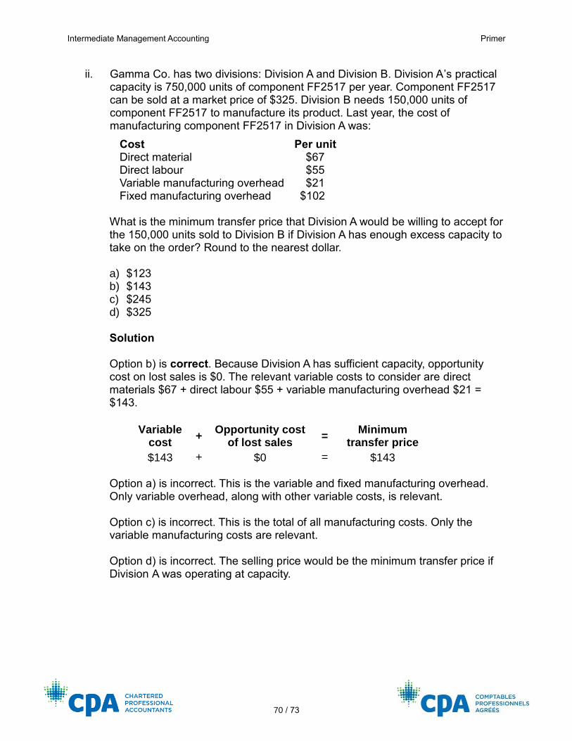
Intermediate Management Accounting Primer
70 / 73
ii. Gamma Co. has two divisions: Division A and Division B. Division A’s practical capacity is 750,000 units of component FF2517 per year. Component FF2517 can be sold at a market price of $325. Division B needs 150,000 units of component FF2517 to manufacture its product. Last year, the cost of manufacturing component FF2517 in Division A was:
Cost Per unit Direct material $67 Direct labour $55 Variable manufacturing overhead $21 Fixed manufacturing overhead $102
What is the minimum transfer price that Division A would be willing to accept for the 150,000 units sold to Division B if Division A has enough excess capacity to take on the order? Round to the nearest dollar.
a) $123 b) $143 c) $245 d) $325
Solution Option b) is correct. Because Division A has sufficient capacity, opportunity cost on lost sales is $0. The relevant variable costs to consider are direct materials $67 + direct labour $55 + variable manufacturing overhead $21 = $143.
Variable cost
+ Opportunity cost
of lost sales =
Minimum transfer price
$143 + $0 = $143 Option a) is incorrect. This is the variable and fixed manufacturing overhead. Only variable overhead, along with other variable costs, is relevant. Option c) is incorrect. This is the total of all manufacturing costs. Only the variable manufacturing costs are relevant. Option d) is incorrect. The selling price would be the minimum transfer price if Division A was operating at capacity.
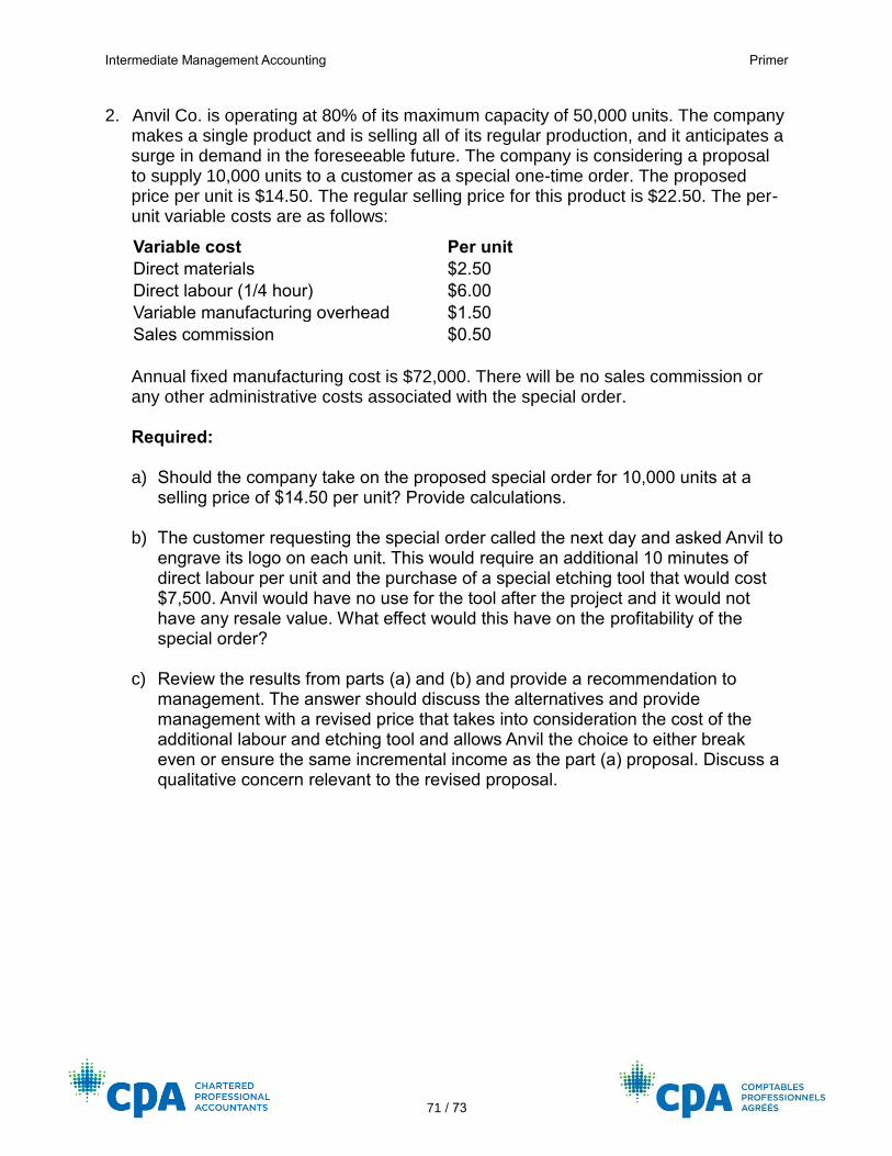
Intermediate Management Accounting Primer
71 / 73
2. .Anvil Co. is operating at 80% of its maximum capacity of 50,000 units. The company makes a single product and is selling all of its regular production, and it anticipates a surge in demand in the foreseeable future. The company is considering a proposal to supply 10,000 units to a customer as a special one-time order. The proposed price per unit is $14.50. The regular selling price for this product is $22.50. The per-unit variable costs are as follows:
Variable cost Per unit
Direct materials $2.50
Direct labour (1/4 hour) $6.00
Variable manufacturing overhead $1.50
Sales commission $0.50
Annual fixed manufacturing cost is $72,000. There will be no sales commission or any other administrative costs associated with the special order. Required:
a) Should the company take on the proposed special order for 10,000 units at a
selling price of $14.50 per unit? Provide calculations.
b) The customer requesting the special order called the next day and asked Anvil to engrave its logo on each unit. This would require an additional 10 minutes of direct labour per unit and the purchase of a special etching tool that would cost $7,500. Anvil would have no use for the tool after the project and it would not have any resale value. What effect would this have on the profitability of the special order?
c) Review the results from parts (a) and (b) and provide a recommendation to management. The answer should discuss the alternatives and provide management with a revised price that takes into consideration the cost of the additional labour and etching tool and allows Anvil the choice to either break even or ensure the same incremental income as the part (a) proposal. Discuss a qualitative concern relevant to the revised proposal.
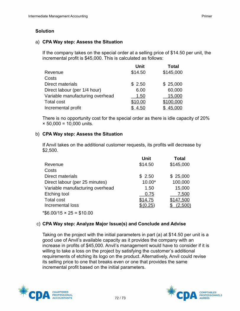
Intermediate Management Accounting Primer
72 / 73
Solution
a) CPA Way step: Assess the Situation If the company takes on the special order at a selling price of $14.50 per unit, the incremental profit is $45,000. This is calculated as follows:
Unit Total
Revenue $14.50 $145,000
Costs
Direct materials $ 2.50 $ 25,000
Direct labour (per 1/4 hour) 6.00 60,000
Variable manufacturing overhead 1.50 15,000
Total cost $10.00 $100,000
Incremental profit $ 4.50 $ 45,000
There is no opportunity cost for the special order as there is idle capacity of 20% × 50,000 = 10,000 units.
b) CPA Way step: Assess the Situation If Anvil takes on the additional customer requests, its profits will decrease by $2,500.
Unit Total
Revenue $14.50 $145,000
Costs
Direct materials $ 2.50 $ 25,000
Direct labour (per 25 minutes) 10.00* 100,000
Variable manufacturing overhead 1.50 15,000
Etching tool 0.75 7,500
Total cost $14.75 $147,500 Incremental loss $ (0.25) $ (2,500)
*$6.00/15 × 25 = $10.00
c) CPA Way step: Analyze Major Issue(s) and Conclude and Advise Taking on the project with the initial parameters in part (a) at $14.50 per unit is a good use of Anvil’s available capacity as it provides the company with an increase in profits of $45,000. Anvil’s management would have to consider if it is willing to take a loss on the project by satisfying the customer’s additional requirements of etching its logo on the product. Alternatively, Anvil could revise its selling price to one that breaks even or one that provides the same incremental profit based on the initial parameters.
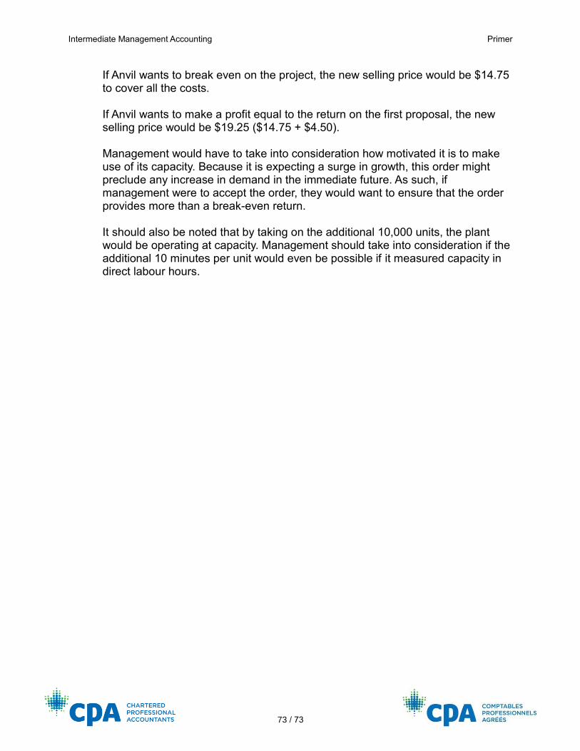
Intermediate Management Accounting Primer
73 / 73
If Anvil wants to break even on the project, the new selling price would be $14.75 to cover all the costs. If Anvil wants to make a profit equal to the return on the first proposal, the new selling price would be $19.25 ($14.75 + $4.50). Management would have to take into consideration how motivated it is to make use of its capacity. Because it is expecting a surge in growth, this order might preclude any increase in demand in the immediate future. As such, if management were to accept the order, they would want to ensure that the order provides more than a break-even return. It should also be noted that by taking on the additional 10,000 units, the plant would be operating at capacity. Management should take into consideration if the additional 10 minutes per unit would even be possible if it measured capacity in direct labour hours.