Embed Size (px)
Citation preview
Intermediate Macroeconomics, EC2201
L8: The open economy
Anna Seim
Department of Economics, Stockholm University
Spring 2018
1 / 47
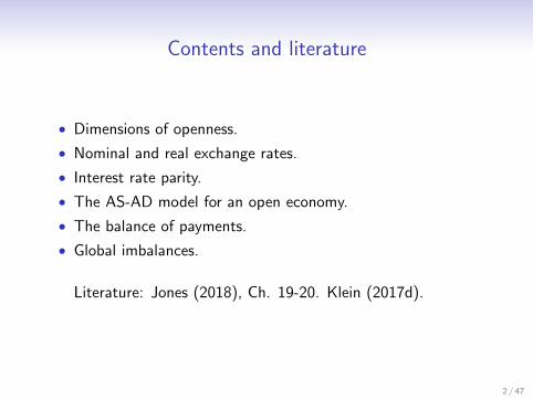
Contents and literature
• Dimensions of openness.
• Nominal and real exchange rates.
• Interest rate parity.
• The AS-AD model for an open economy.
• The balance of payments.
• Global imbalances.
Literature: Jones (2018), Ch. 19-20. Klein (2017d).
2 / 47
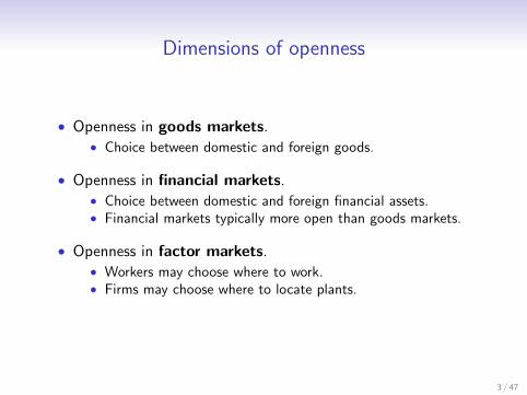
Dimensions of openness
• Openness in goods markets.• Choice between domestic and foreign goods.
• Openness in financial markets.• Choice between domestic and foreign financial assets.• Financial markets typically more open than goods markets.
• Openness in factor markets.• Workers may choose where to work.• Firms may choose where to locate plants.
3 / 47
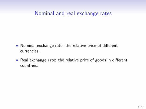
Nominal and real exchange rates
• Nominal exchange rate: the relative price of differentcurrencies.
• Real exchange rate: the relative price of goods in differentcountries.
4 / 47
Nominal exchange rates
Express the (spot) nominal exchange rate, E , in foreign currency(euro, e) per unit of domestic currency (SEK).
Will use this definition throughout the course to stay consistentwith Jones (2018).
∆E > 0: an appreciation (revaluation) of the krona.
∆E < 0: a depreciation (devaluation) of the krona.
5 / 47

The nominal Swedish exchange rate, February 20, 2018
Domestic currency/ Foreign currency/Foreign currency foreign currency domestic currency
EURO 9.97 0.10
USD 8.07 0.12
GBP 11.29 0.09
NOK 1.03 0.97
6 / 47

The real exchange rate
The real exchange rate, Q, is defined:
Q =EP
P∗, (1)
where P denotes the price level and ∗ henceforth indicates foreign.
Real appreciation: ∆Q > 0. Domestic goods become relativelymore expensive.
Real depreciation: ∆Q < 0. Domestic goods become relativelycheaper.
7 / 47
Real exchange rate dynamics
• Since prices tend to be sticky, the relative price, P/P∗, maybe treated as given in the short run.
• Understanding nominal exchange rates therefore key tounderstanding the real exchange rate in the short run.
8 / 47
The nominal exchange rate in the short run
• Asset-market approach.
• Nominal exchange rate governed by an Interest Rate Paritycondition.
9 / 47
The foreign exchange market
• The nominal exchange rate: a financial asset.
• Determined by the interaction of buyers and sellers in theforeign exchange market.
• Trading agents:
• Commercial banks (interbank trading).
• Multinational corporations.
• Non-bank financial institutions (pension funds, hedge funds).
• Central banks.
10 / 47
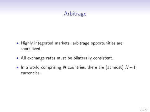
Arbitrage
• Highly integrated markets: arbitrage opportunities areshort-lived.
• All exchange rates must be bilaterally consistent.
• In a world comprising N countries, there are (at most) N−1currencies.
11 / 47
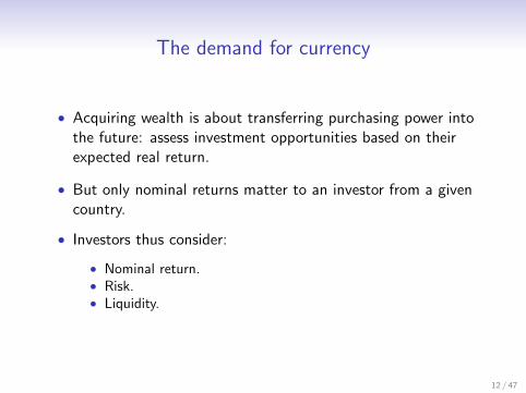
The demand for currency
• Acquiring wealth is about transferring purchasing power intothe future: assess investment opportunities based on theirexpected real return.
• But only nominal returns matter to an investor from a givencountry.
• Investors thus consider:
• Nominal return.• Risk.• Liquidity.
12 / 47
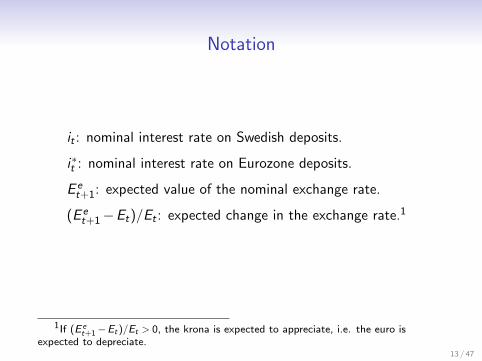
Notation
it : nominal interest rate on Swedish deposits.
i∗t : nominal interest rate on Eurozone deposits.
E et+1: expected value of the nominal exchange rate.
(E et+1−Et)/Et : expected change in the exchange rate.1
1If (E et+1−Et)/Et > 0, the krona is expected to appreciate, i.e. the euro is
expected to depreciate.13 / 47
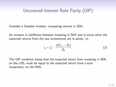
Uncovered Interest Rate Parity (UIP)
Consider a Swedish investor, comparing returns in SEK.
An investor is indifferent between investing in SEK and in euros when theexpected returns from the two investments are in parity, i.e.:
it = i∗t −(E e
t+1−Et)
Et. (2)
The UIP condition states that the expected return from investing in SEK,on the LHS, must be equal to the expected return from a euroinvestment, on the RHS.
14 / 47
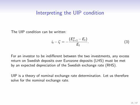
Interpreting the UIP condition
The UIP condition can be written:
it − i∗t =−(E e
t+1−Et)
Et. (3)
For an investor to be indifferent between the two investments, any excessreturn on Swedish deposits over Eurozone deposits (LHS) must be metby an expected depreciation of the Swedish exchange rate (RHS).
UIP is a theory of nominal exchange rate determination. Let us thereforesolve for the nominal exchange rate.
15 / 47
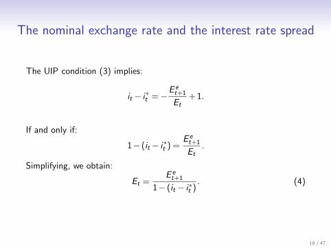
The nominal exchange rate and the interest rate spread
The UIP condition (3) implies:
it − i∗t =−E et+1
Et+ 1.
If and only if:
1− (it − i∗t ) =E et+1
Et.
Simplifying, we obtain:
Et =E et+1
1− (it − i∗t ). (4)
16 / 47
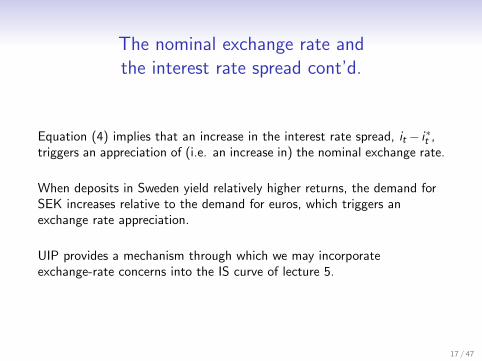
The nominal exchange rate andthe interest rate spread cont’d.
Equation (4) implies that an increase in the interest rate spread, it − i∗t ,triggers an appreciation of (i.e. an increase in) the nominal exchange rate.
When deposits in Sweden yield relatively higher returns, the demand forSEK increases relative to the demand for euros, which triggers anexchange rate appreciation.
UIP provides a mechanism through which we may incorporateexchange-rate concerns into the IS curve of lecture 5.
17 / 47
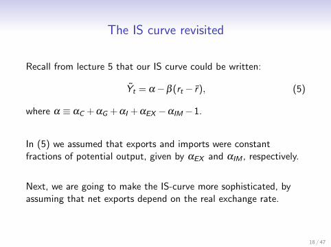
The IS curve revisited
Recall from lecture 5 that our IS curve could be written:
Yt = α−β (rt − r), (5)
where α ≡ αC + αG + αI + αEX −αIM −1.
In (5) we assumed that exports and imports were constantfractions of potential output, given by αEX and αIM , respectively.
Next, we are going to make the IS-curve more sophisticated, byassuming that net exports depend on the real exchange rate.
18 / 47

National income in the open economy revisited
Recall from lecture 5, that in the open economy, the nationalincome identity is given by:
Yt = Ct + It +Gt +NXt . (6)
where NXt ≡ EXt − IMt .
Next, we will assume:
NXt
Yt= αNX −βNX (rt − r∗t ), (7)
where rt is the domestic real interest rate and r∗t is the foreign realinterest rate.
19 / 47
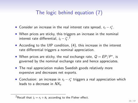
The logic behind equation (7)
• Consider an increase in the real interest rate spread, rt − r∗t .
• When prices are sticky, this triggers an increase in the nominalinterest rate differential, it − i∗t .2
• According to the UIP condition, (4), this increase in the interestrate differential triggers a nominal appreciation.
• When prices are sticky, the real exchange rate, Q = EP/P∗, isgoverned by the nominal exchange rate and hence appreciates.
• The real appreciation makes Swedish goods relatively moreexpensive and decreases net exports.
• Conclusion: an increase in rt − r∗t triggers a real appreciation whichleads to a decrease in NXt .
2Recall that it = rt + πt according to the Fisher effect.20 / 47
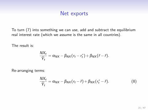
Net exports
To turn (7) into something we can use, add and subtract the equilibriumreal interest rate (which we assume is the same in all countries).
The result is:
NXt
Yt= αNX −βNX (rt − r∗t ) + βNX (r − r).
Re-arranging terms:
NXt
Yt= αNX −βNX (rt − r) + βNX (r∗t − r). (8)
21 / 47
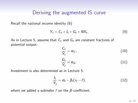
Deriving the augmented IS curve
Recall the national income identity (6)
Yt = Ct + It +Gt +NXt . (9)
As in Lecture 5, assume that Ct and Gt are constant fractions ofpotential output:
Ct
Yt= αC , (10)
Gt
Yt= αG . (11)
Investment is also determined as in Lecture 5:
It
Yt= αI −βI (rt − r), (12)
where we added a subindex I on the β -coefficient.
22 / 47
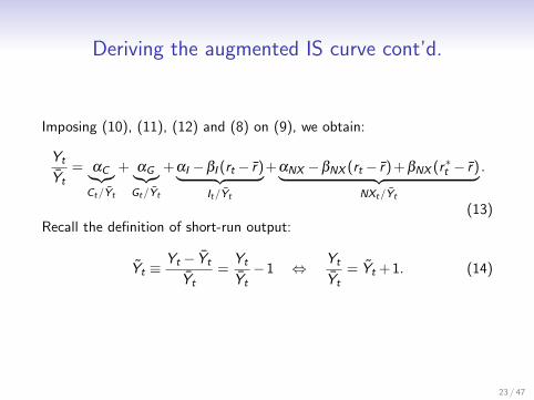
Deriving the augmented IS curve cont’d.
Imposing (10), (11), (12) and (8) on (9), we obtain:
Yt
Yt= αC︸︷︷︸
Ct/Yt
+ αG︸︷︷︸Gt/Yt
+αI −βI (rt − r)︸ ︷︷ ︸It/Yt
+αNX −βNX (rt − r) + βNX (r∗t − r)︸ ︷︷ ︸NXt/Yt
.
(13)Recall the definition of short-run output:
Yt ≡Yt − Yt
Yt=
Yt
Yt−1 ⇔ Yt
Yt= Yt + 1. (14)
23 / 47
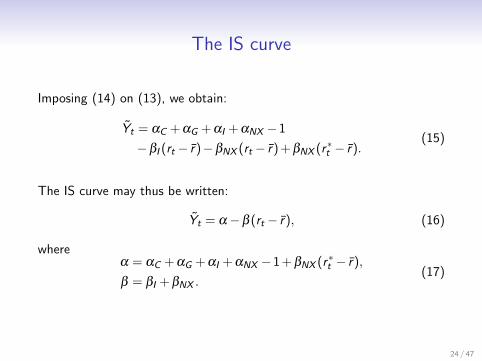
The IS curve
Imposing (14) on (13), we obtain:
Yt = αC + αG + αI + αNX −1
−βI (rt − r)−βNX (rt − r) + βNX (r∗t − r).(15)
The IS curve may thus be written:
Yt = α−β (rt − r), (16)
whereα = αC + αG + αI + αNX −1 + βNX (r∗t − r),
β = βI + βNX .(17)
24 / 47

Interpreting the IS curve
As before, α = 0, and rt = r in the long run, so that Yt = 0 in long-runequilibrium.
The IS curve (16) is very similar to the one in the closed economy, butthe model is richer: α and β contain more parameters that can besubjected to shocks.
In particular, a shock to the foreign interest rate, r∗t , is a positive demandshock since it causes a depreciation of the domestic exchange rate, whichincreases net exports.
25 / 47
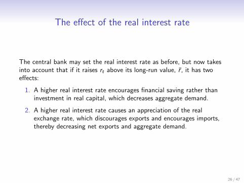
The effect of the real interest rate
The central bank may set the real interest rate as before, but now takesinto account that if it raises rt above its long-run value, r , it has twoeffects:
1. A higher real interest rate encourages financial saving rather thaninvestment in real capital, which decreases aggregate demand.
2. A higher real interest rate causes an appreciation of the realexchange rate, which discourages exports and encourages imports,thereby decreasing net exports and aggregate demand.
26 / 47

Fig. 20.4
Extracted from: Jones (2018).
27 / 47
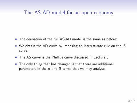
The AS-AD model for an open economy
• The derivation of the full AS-AD model is the same as before:
• We obtain the AD curve by imposing an interest-rate rule on the IScurve.
• The AS curve is the Phillips curve discussed in Lecture 5.
• The only thing that has changed is that there are additionalparameters in the α and β -terms that we may analyse.
28 / 47
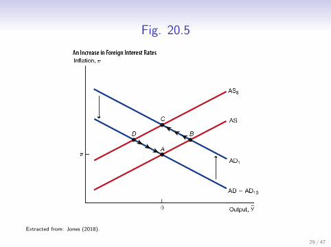
Fig. 20.5
Extracted from: Jones (2018).
29 / 47
The national income identity revisited
Recall the national income identity, (6), repeated here forconvenience:
Yt = Ct + It +Gt +NXt . (18)
Adding and subtracting taxes, Tt , from (18) and re-arranging:(Yt −Tt −Ct
)︸ ︷︷ ︸
SP
+
(Tt −Gt
)︸ ︷︷ ︸
SG
= It +NXt , (19)
where SP and SG denote private and government saving,respectively.
30 / 47
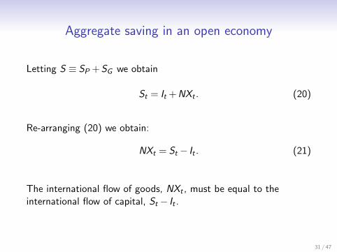
Aggregate saving in an open economy
Letting S ≡ SP +SG we obtain
St = It +NXt . (20)
Re-arranging (20) we obtain:
NXt = St − It . (21)
The international flow of goods, NXt , must be equal to theinternational flow of capital, St − It .
31 / 47
Saving and investment in a closed economy
Consider a closed economy where NXt = 0. This implies:
It = St .
In a closed economy, investment must equal saving.3
In an open economy, countries may run trade deficits by borrowingfrom abroad according to (21).
3Hence the name, ”IS curve”.32 / 47
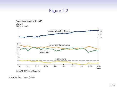
Figure 2.2
Extracted from: Jones (2018).
33 / 47
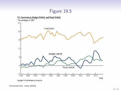
Figure 19.5
Extracted from: Jones (2018).
34 / 47
Keeping track of international transactions
• Goods markets and financial markets closely connected toeach other.
• All transactions with the rest of the world (ROW) aredocumented in a country’s balance of payments.
35 / 47
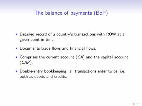
The balance of payments (BoP)
• Detailed record of a country’s transactions with ROW at agiven point in time.
• Documents trade flows and financial flows.
• Comprises the current account (CA) and the capital account(CAP).
• Double-entry bookkeeping: all transactions enter twice, i.e.both as debits and credits.
36 / 47
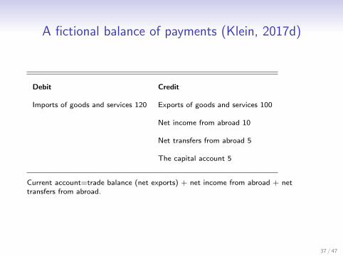
A fictional balance of payments (Klein, 2017d)
Debit Credit
Imports of goods and services 120 Exports of goods and services 100
Net income from abroad 10
Net transfers from abroad 5
The capital account 5
Current account=trade balance (net exports) + net income from abroad + nettransfers from abroad.
37 / 47
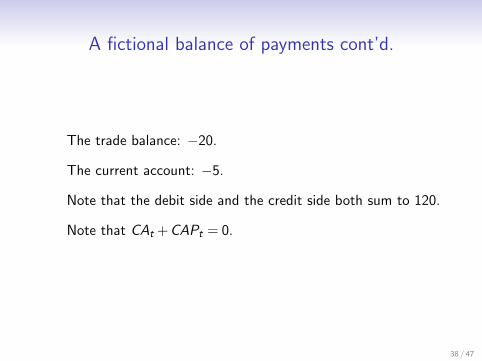
A fictional balance of payments cont’d.
The trade balance: −20.
The current account: −5.
Note that the debit side and the credit side both sum to 120.
Note that CAt +CAPt = 0.
38 / 47
What determines the current account?
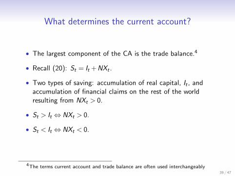
• The largest component of the CA is the trade balance.4
• Recall (20): St = It +NXt .
• Two types of saving: accumulation of real capital, It , andaccumulation of financial claims on the rest of the worldresulting from NXt > 0.
• St > It ⇔ NXt > 0.
• St < It ⇔ NXt < 0.
4The terms current account and trade balance are often used interchangeably39 / 47
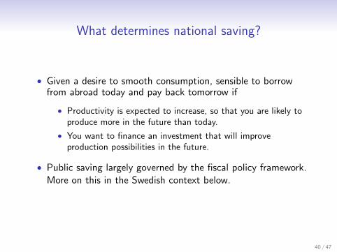
What determines national saving?
• Given a desire to smooth consumption, sensible to borrowfrom abroad today and pay back tomorrow if
• Productivity is expected to increase, so that you are likely toproduce more in the future than today.
• You want to finance an investment that will improveproduction possibilities in the future.
• Public saving largely governed by the fiscal policy framework.More on this in the Swedish context below.
40 / 47
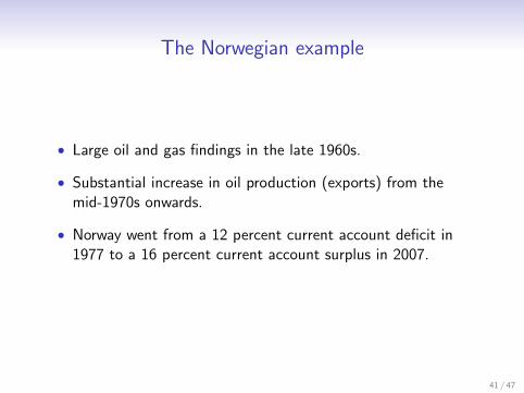
The Norwegian example
• Large oil and gas findings in the late 1960s.
• Substantial increase in oil production (exports) from themid-1970s onwards.
• Norway went from a 12 percent current account deficit in1977 to a 16 percent current account surplus in 2007.
41 / 47
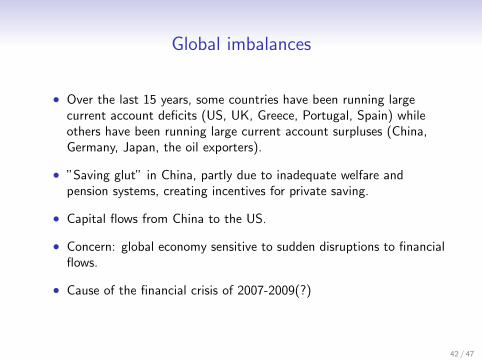
Global imbalances
• Over the last 15 years, some countries have been running largecurrent account deficits (US, UK, Greece, Portugal, Spain) whileothers have been running large current account surpluses (China,Germany, Japan, the oil exporters).
• ”Saving glut” in China, partly due to inadequate welfare andpension systems, creating incentives for private saving.
• Capital flows from China to the US.
• Concern: global economy sensitive to sudden disruptions to financialflows.
• Cause of the financial crisis of 2007-2009(?)
42 / 47
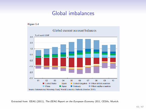
Global imbalances
Extracted from: EEAG (2011), The EEAG Report on the European Economy 2011, CESifo, Munich.
43 / 47
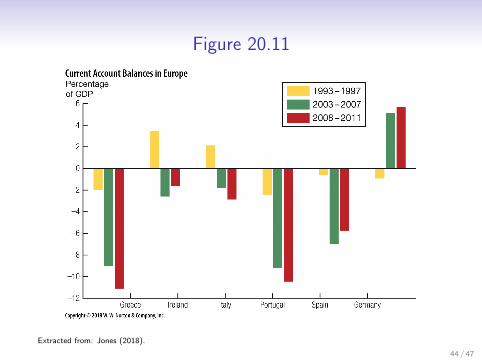
Figure 20.11
Extracted from: Jones (2018).
44 / 47

Extracted from: Vredin, A., Floden, M. Larsson, A. and Ravn, M.O. (2012), Simple Rules, Difficult Times,Economic Policy Group Report 2012, SNS Forlag.
45 / 47
The Swedish current account
• Large current account deficits prior to the crisis in the 1990s.
• Eliminated by large nominal (and real) depreciation when thefixed exchange rate was abandoned in 1992.
• Large current account surpluses from the mid 1990s onwards,largely due to fiscal consolidation.
• Note: Details on the Swedish fiscal framework in Lecture 7.More on exchange rates in Lecture 9.
46 / 47
Contents and literature
• Dimensions of openness.
• Nominal and real exchange rates.
• Interest rate parity.
• The AS-AD model for an open economy.
• The balance of payments.
• Global imbalances.
Literature: Jones (2018), Ch. 19-20. Klein (2017d).
Next time: Exchange rates.
47 / 47