Embed Size (px)
Citation preview

International Institute for Applied Systems Analysis Schlossplatz 1 A-2361 Laxenburg, Austria
Tel: +43 2236 807 342 Fax: +43 2236 71313
E-mail: [email protected] Web: www.iiasa.ac.at
Interim Reports on work of the International Institute for Applied Systems Analysis receive only limited review. Views or opinions expressed herein do not necessarily represent those of the Institute, its National Member Organizations, or other organizations supporting the work.
Interim Report IR-02-33
An Economic Model of International Gas Pipeline Routings to the Turkish Market: Numerical results for an uncertain future Olga Golovina ([email protected], [email protected]) Ger Klaassen ([email protected]) R. Alexander Roehrl
Approved by
Leo Schrattenholzer ([email protected]): Project leader, Environmentally Compatible Energy Strategies (ECS) Project
July 2002

ii
Contents
1. INTRODUCTION ........................................................................................................................1 2. DATA.............................................................................................................................................3 3. DESCRIPTION OF THE MODEL ............................................................................................6
3.1. OBJECTS AND PARAMETERS ....................................................................................................6 3.2. DYNAMICS OF INVESTMENTS ..................................................................................................7 3.3. DYNAMICS OF GAS SUPPLY......................................................................................................8 3.4. PRICE FORMATION MECHANISM AND REVENUES DUE TO GAS SALES......................................9 3.5. PROFITS .................................................................................................................................10
4. SIMULATION RESULTS.........................................................................................................10 4.1 CASE A: MOVING TOWARD A LIBERALIZED TURKISH ENERGY MARKET (HIGH PRICE
ELASTICITY)..................................................................................................................................11 4.1.1. Case A, scenario 1: Commercialization times for all pipelines as currently planned...11 4.1.2. Case A, scenario 2: Blue Stream’s commercialization time optimized. Other pipelines as planned ................................................................................................................................13 4.1.3. Case A, scenario 3: Trans-Caspian’s commercialization time optimized. Other pipelines as planned.................................................................................................................13 4.1.4. Case A, scenario 4: Iranpipe’s commercialization time optimized. Other pipelines as planned.....................................................................................................................................14 4.1.5. Case A, scenario 5: Nash equilibrium in a game between the pipelines .......................14
4.2. CASE B: PARAMETERS AS IN TYPICAL EMERGING GAS MARKETS (LOWER PRICE ELASTICITY)......................................................................................................................................................16
4.2.1 Case B, scenario 1: Commercialization times for all pipelines as currently planned....16 4.2.2. Case B, scenarios 2-5: Commercialization times optimized (various cases) ................18
5. SENSITIVITY ANALYSES ......................................................................................................19 5.1. SENSITIVITY FOR THE GDP ELASTICITY OF DEMAND, SCENARIO 1 (ALL
COMMERCIALIZATION TIMES AS CURRENTLY PLANNED) .............................................................19 5.2. SENSITIVITY OF THE RESULTS FOR THE PRICE ELASTICITY OF DEMAND, SCENARIO 1 (ALL
COMMERCIALIZATION TIMES AS CURRENTLY PLANNED) .............................................................20 5.3. SENSITIVITY OF THE RESULTS FOR CHANGES IN THE DISCOUNT RATE, SCENARIO 1 (ALL
COMMERCIALIZATION TIMES AS CURRENTLY PLANNED) .............................................................21 5.4. SENSITIVITY FOR GDP ELASTICITY OF DEMAND, SCENARIO 5 (NASH EQUILIBRIUM) ..........22 5.5. SENSITIVITY FOR PRICE ELASTICITY OF DEMAND, SCENARIO 5 (NASH EQUILIBRIUM) .........23 5.6. SENSITIVITY FOR THE DISCOUNT RATE, SCENARIO 5 (NASH EQUILIBRIUM) .........................24
6. CONCLUSIONS.........................................................................................................................25 APPENDIX......................................................................................................................................26 REFERENCES ...............................................................................................................................30

iii
Abstract
This paper presents a dynamic investment model of the international gas pipeline routings to the Turkish market. The model was developed by IIASA’s Dynamic Systems Project (DYN) and Environmentally Compatible Energy Strategies Project (ECS) in 2000. To allow for user-friendly modeling, a professional software package “Investments in gas Pipelines Optimization of Returns” (IGOR) was developed which can also be used as a basis for models for related problems. Input data originated from various sources, in particular IIASA’s MESSAGE model. The paper analyzes model results under a wide range of future outcomes and includes comprehensive sensitivity analyses. The returns for five potential gas pipeline projects were analyzed for a wide range of values for the price elasticity of gas demand, GDP elasticity of gas demand and discount rates. The numerical results allow conclusions about gas price developments and optimal gas supply policies relative to the market parameters.

iv
Acknowledgments and Disclaimer
The authors are thankful to Alexander Tarasyev and Ivan Matrosov for their help in carrying out the numerical analysis and to Arkadii Kryazhimskii for useful editorial comments. Comments from Leo Schrattenholzer on an earlier draft are appreciated.

v
About the Authors
Olga Golovina is a postgraduate student at the Faculty of Numerical Mathematics and Cybernetics, Moscow State University. In 2001 she participated in IIASA’s Young Scientists Summer Program. Her work was supervised by the IIASA’s Dynamic Systems Project and Environmentally Compatible Energy Strategies Project.
Ger Klaassen is a Senior Research Scholar at IIASA’s Environmentally Compatible Energy Strategies Project.
R. Alexander Roehrl was a Research Scholar with IIASA’s Environmentally Compatible Energy Strategies Project from September 1997 to December 2000.

1
An economic model of international gas pipeline routings to the Turkish market – Numerical results for an uncertain future
Olga Golovina∗∗∗∗ , Ger Klaassen, and R. Alexander Roehrl
1. Introduction
The following extract from the United States Energy Information Administration’s country report on Turkey is an excellent summary of the political, economic, geographic, and environmental factors determining future gas pipeline routing to Turkey. It describes the situation as of July 2001:
“There is no more perspective and capacious gas market in Asia and especially Caspian region today than Turkey. Turkey's energy consumption is growing much faster than its production, making Turkey a rapidly growing energy importer. Turkish natural gas demand is projected to increase rapidly in coming years, with the prime consumers expected to be power plants and industrial users. Natural gas is Turkey's preferred fuel for new power plant capacity for several reasons: environmental (gas is cleaner than coal, lignite, or oil); geographic (Turkey is close to huge amounts of gas in the Middle East and Central Asia); economic (Turkey could offset part of its energy import bill through transit fees it could charge for oil and gas shipments across its territory); and political (Turkey is seeking to strengthen relations with Caspian and Central Asian countries, several of which are potentially large gas exporters).
Around 70% of current Turkish gas imports come from Russia via the trans-Balkan pipeline, with the other 30% coming mainly from Algeria and Nigeria via LNG tanker. Turkey has signed (or discussed) gas import deals with a variety of countries, including Azerbaijan, Egypt, Iran, Iraq, Russia, and Turkmenistan (see Figure 1). For gas exports beginning in 2004 around 40% is expected to come from Russia via Bulgaria, with 33% supplied from Russia via the Black Sea, 17% from Iran, and 8% from Azerbaijan.
On December 15, 1997, Russia and Turkey signed a 25-year deal under which the Russian gas company, Gazprom, would construct a new gas export pipeline (called "Blue Stream") to Turkey for delivery capacity of around 565 Bcf annually, with initial deliveries possibly starting in 2002. The $2.7-$3.2 billion, 758-mile dual pipeline is slated to run from Izobilnoye in southern Russia, to Dzhugba on the Black Sea, then under the Black Sea for about 247 miles to the Turkish port of Samsun, and on to Ankara. When completed, possibly by early 2002, the Blue Stream lines will be the world's deepest underwater gas pipelines, and will require complex engineering to construct the pipeline. The two main companies involved in Blue Stream are Russia's Gazprom and Italy's ENI SpA.
Turkey's most controversial gas import deal is one with Iran, signed in 1996. Under this 23-year arrangement, Iran will supply Turkey with gas, mainly from the Kangan gas field in the south and the Khangiran gas field in the northeast. Iran also imports gas from Turkmenistan, and could
∗ This author was partially supported by the Russian Foundation of Basic Research under grant #00-01-00682

2
send spare volumes to Turkey as well. In January 2000, Turkey and Iran announced agreement on postponing the 23-year gas deal's start to July 2001, more than a year behind schedule, purportedly due to lack of completion of two pipeline stages in Turkey (U.S. opposition to Turkey's deal with Iran may also have been a factor). In late June 2001, the gas deal was delayed once again. But Turkey has steadfastly maintained that it needs to diversify its suppliers of natural gas away from Russia and that Turkmen and Iranian gas represent economically sound alternatives.
Figure 1. Gas pipeline routes to Turkey (Source: Gas Matters)
On May 21, 1999, Botas signed an agreement on building a $2-$2.4 billion, 1,050-mile, gas pipeline from Turkmenistan, underneath the Caspian Sea, across Azerbaijan and Georgia (both of which would collect transit fees), and on to Turkey. The consortium is led by U.S. company Bechtel and including General Electric, Shell, and PSG International. Despite previous Turkish government statements that a gas pipeline from Turkmenistan was a top priority, this now seems highly unlikely, as it would compete against the proposed Blue Stream project, as well as against possible gas supplies from Iran. Progress on the TCP (Trans-Caspian) appears stalled at the moment, with the international consortium essentially having suspended operations, while Blue Stream appears to be proceeding. That is why now the possibility of exporting more of Turkmen gas to Russia is discussed.” 1
Recent information on the progress in building the “Bluestream” pipeline suggests that the ENI has finished laying the first of two lines. The second line is expected to be completed by the end of 2002 (Anonymous, 2002). No start date for deliveries of gas has been fixed but these deliveries are expected to build up to 7 billion cm in 2004 and to reach a plateau of 16 billion cm in 2007. Turkey’s gas company Botas expects deliveries of 6 billion cm in 2004 and foresee the plateau to be reached in 2009) (Quinlan, 2002).
Against this background the present paper focuses on Turkey. We use a new dynamic model described in terms of differential equations to analyze possible scenarios of investments in international Turkey-oriented gas pipelines. The results of the sensitivity analysis give us a better understanding of which outcomes of the pipeline projects performance may be most sensitive/robust to variation in their parameters and changes on the Turkish gas market.
1 EIA (2001) Turkey. July 2001. United States Energy Information Administration. Washington.
Bolgarpipe
Blue Stream
Ekarum
Transcaspian
Iranpipe

3
The paper is organized as follows. Section 2 describes the input data. Section 3 introduces the model. Section 4 presents results of model-and-data-based numerical simulations under different optimization scenarios. Section 5 presents results of a numerical sensitivity analysis of the Turkish gas market. Section 6 concludes.
2. Data
In this paper, we focus attention on five possible gas export pipelines to the Turkey market:
− “Trans-Balkan”. This is the only currently operational pipeline. Natural gas is delivered via Ukraine, Romania and Bulgaria to Turkey.
− “Blue Stream”. This project proposes a direct connection between Russia and Turkey under the Black Sea. It will probably be completed in 2002.
− “Trans-Caspian”. This pipeline is planned to deliver gas from Turkmenistan to Turkey through Azerbaijan and Georgia.
− “Ekarum”. This partially completed pipeline is proposed to import gas from Turkmenistan to Iran and then to Turkey.
− “Iranpipeline”. This pipeline goes directly from Iran. It is an alternative to the “Blue Stream”.
Table 1 presents the major data on these gas transmission lines.
Table 1. Data on the Turkey gas market Origin: Russia Russia Turkmenistan Turkmenistan Iran Name: Trans-Balkan Blue Stream Trans-Caspian Ekarum Iranpipe
Gas supply estimated to start by:
exists 2002 2002 2009 2010
Percentage constructed in 1998(%)
100 0 0 54 58
Final capacity (bcm/year)
10.2 14.16 31.15 28.3 28
Length (miles) 3500 1220 1696 2172 2400
Investment (billion US$)
exists 3-4.3 2-3 3.8-4 3.9-4.1
Transportation costs (million US$/bcm)
30 14.1 8 30 30
Distribution Costs (million US$/bcm)
33 33 33 33 33
Transit fees (million US$/bcm)
10 0 16.9 21.6 0
Some of the data presented in Table 1 were obtained using the IIASA’s MESSAGE model (Roehrl et al., 2000). Data for the start year, capacity, length and investment (construction) costs are based on EIA (1999a and 1999b), Ignatius (2000) and Zhao (2000). Operation and maintenance costs (in our simulations these recurring expenses relate to the transportation costs) are based on data of the MESSAGE model and are equal to 10% of the investment (Strubegger and Messner, 1995). Data for transit fees are estimated on the basis of the existing transit fees from Russia through Ukraine and the length of the transit route (Sagers, 1999). Distribution costs include domestic distribution and storage costs to the residential, industrial and conversion sectors, (Golombek, et al., 1995). We take the averages of these estimates for households and for industry and weigh them with the average consumption of gas for these two sectors in Turkey between 1996 and 1998. This gives an estimate of US$ 33/1000 cm (and a range of 22-57$/1000 cm).

4
The investment costs depend on the time of completing the pipeline, reflecting technical progress as observed for on-shore and offshore pipelines (Zhao, 2000). The earlier is the start year, the higher are the investment costs. For every year the pipeline is finished later the investment costs are lower but at a decreasing rate (see Figure 2).
Figure 2. Investment costs as function of the year in which the pipeline will be built (million US$)
Important components of gas supply are the costs for extraction. We modeled national gas supply curves for Russia, Iran, Turkmenistan and Kazakhstan (CAP) using national data on gas reserves and resources and international data on costs (Rogner, 1997). The resulting gas supply costs are shown in Figure 3. These data are based on the MESSAGE model taking into account domestic demand and export to regions other than Turkey in a dynamics-as-usual scenario.
N a tu r a l G a s E x t r a c t io n C u r v e s (C a t . I -V )
0
2 0
4 0
6 0
0 2 0 ,0 0 0 4 0 ,0 0 0 6 0 ,0 0 0 8 0 ,0 0 0 1 0 0 ,0 0 0 1 2 0 ,0 0 0 1 4 0 ,0 0 0 1 6 0 ,0 0 0
C u m u la t iv e e x tr a c t io n in r e g io n [b c m ]
Ext
ract
ion
cost
s
[US
$/(1
000
cubm
)]
R u s s iaIra n
C e n tra l A s ia nP ro d u c e rs (C A P )
Figure 3. Cumulative gas supply cost curves
Exogenous domestic gas supply from Turkey (which was only around 0.6 bcm in 2000) is ignored for the sake of simplicity. About 30% of natural gas come to Turkey in the form of liquefied natural gas (LNG), mainly from Algeria and Nigeria. Therefore, the price for LNG must
0
1000
2000
3000
4000
5000
6000
2001 2006 2011 2016 2021 2026t
cost
Blue Stream
Transcaspian
Ekarum
Iranpipe

5
be taken into account in the analysis of the Turkey gas market. LNG supply is supposed to be flexible enough to, in principle, supply the whole Turkish market but only at the world market price. The world market price for LNG (see Figure 4) is derived from the IIASA median scenario (B2) developed for the IPCC Special Report on Emission Scenarios (Nakicenovic, et al., 2000).
Figure 4. The world market price for LNG (US$/1000cm)
GDP forecasts for Turkey were derived from the B2 scenario (see Figure 5) assuming that Turkey would follow the same development path in terms of GDP growth rates per capita as the region Middle-East and North Africa (Riahi and Roehrl, 2000).
0
200
400
600
800
1000
1200
2010
2025
2040
t
GD
P
Figure 5. GDP for Turkey (billion US$)
Using different estimates for the price elasticity (Komiyama, 2000) we study two central cases, A and B.
Case A assumes a price elasticity of –0.7 and a GDP elasticity of 1.25. The GDP elasticity fits with the GDP elasticity in developing countries (see Komiyama, 2000). The price elasticity fits with Turkish data and Turkey’s intention to liberalize energy markets.
Case B assumes a price elasticity of –0.3 and a GDP elasticity of 1.25, which is more in line with the evidence for emerging gas markets.

6
3. Description of the model
This section describes the model that was used for the numerical analysis of the Turkish gas market using the data presented in the previous section. The model was originally suggested in Roehrl et al. (2000) and Matrosov (2000).
3.1. Objects and parameters
The main objects in the model (see Figure 6) are a gas market, a collection of gas fields and a collection of pipelines connecting the gas fields to the market. The gas market is characterized by the GDP level, GDP elasticity of demand, price of gas and price elasticity of demand. Each gas field is characterized by the overall cost of delivering a unit of gas to the market.
The initial period in the lifetime of a gas pipeline project is the period of its construction (the investment period). As soon as the accumulated investment reaches the minimum level needed to start gas supply, gas is delivered to the market. Generally, a pipeline can supply gas at different capacities. The capacity of a pipeline depends on the accumulated capital invested in the project. Further investments enlarge the capacity via either building a new pipeline in parallel to the existing one, or upgrading the pipeline to a higher pressure. In the model, the goal of every project is to maximize profit through regulating the timing of and level of investments, choosing appropriate levels of gas supply and finding an optimal time to start exploitation.
Figure 6. Schematic outline of the model
Gas field 1 (overall costs of delivering gas to
the market)
Gas market
Price of gas
GDP
Price elasticity of
demand
GDP elasticity of
demand
Investment into pipeline 1
Investment into pipeline N
Investment into pipeline 2
Gas field 2 (overall costs of delivering gas to
the market)
Gas field N (overall costs of delivering gas to
the market)
supply supply supply

7
The model employs the following set of parameters ( t denotes current time (year)).
Constants: N the number of the pipelines;
0t initial time (time to start investments, common for all pipelines);
σ the obsolescence coefficient (one divided by the lifetime); γ the time-delay exponential coefficient.
Parameters of pipeline i ( Ni ,...,1= ):
iK the number of capacity levels;
kix level of the accumulated investment needed to start supply at capacity level
k ( iKk ,...,0= );
kiM maximum capacity for capacity level k ( iKk ,...,0= );
kit time (year) to start exploitation at capacity level k;
lit final time;
)(tkir current investment enlarging capacity from level k-1 to level k;
)(tix current accumulated investment;
)(tiy current supply;
)(tiy current accumulated supply;
)(tiC current overall cost of delivering a unit of gas.
Market parameters:
ey GDP elasticity of demand; ep price elasticity of demand;
λ discount rate; G(t) GDP, national income; P(t) price of gas; PLNG(t) price of LNG.
3.2. Dynamics of investments
The dynamics of accumulated investments, )(tix , in pipeline i during the investment period
is described by

8
)()()( tirtixtix γσ +−=& ;
here σ is the obsolescence coefficient (σ >0), γ the discount return coefficient (0<γ <1)
and )()( tkirtir = the current investment level in the capacity level k-1.
If for pipeline i the times kit to start supply at capacity levels iKk ,...2,1=
are fixed
(published building plans can be used to estimate kit ), the maximization of the profit for pipeline i
is synonymous to the minimization of its investment cost and maximization of supply. The
minimum cost for enlarging the pipeline’s capacity from level 1−k to level k is found as
where 0
0 ti
t = and λ is the discount rate.
An argument from the mathematical control theory yields the following formula for the
optimal investment policy, )(tkir :
with
1−+= α
λασρ , 11 >=γ
α .
3.3. Dynamics of gas supply
For pipeline i, the dynamics of gas supply, )(tyi , at the maximum capacity kiM for the
capacity level k is modeled by
+−+−=
)(
)()())(()(
tidy
tidRsigntiyk
iMsigntiysignQtiy& ;
dsskir
kit
kit
sekir
kiW )(
1)(min ∫
−−
⋅= λ
α
ρρ
σσ
ρ
−−−
−
−−−−
−
=)1()(
1)1()(
)(tk
itetk
ite
kix
tkitek
ixtk
itetk
ir
(1)
(2)
(3)
(4)
(5)

9
here Q is a (large) positive parameter characterizing the ability of the managers of the pipeline to regulate supply depending on changes on the market, and Ri (t) is the revenues due to sales of gas. A solution to this equation approximates supply for pipeline i at currently emerging instantaneous equilibria on the gas market (see Klaassen, et al., 2000).
If the share of LNG in the gas market is high enough (which is the case for the Turkish market), it is necessary to include LNG in the model. We assume that the price for LNG, PLNG(t), on the world market is a given function of time. This gives us a similar equation for LNG supply:
( ) ( ) ( )
−+−+−= )()()()()( t
LNGPtPsignt
LNGy
LNGMsignt
LNGysignQtLNGy&
where MLNG is the maximum capacity of LNG terminals. The price for LNG serves as an upper bound for the price for gas.
3.4. Price formation mechanism and revenues due to gas sales
One finds the current price for gas by equalizing the current demand and supply on the gas market. Current demand, )(tD , is a function of price, P(t), and GDP, G(t):
petPye
tGAtD−
= ))(())(()( ;
here A is a scale coefficient, ey is the GDP elasticity of demand and ep is the price elasticity of demand. The current supply, )(tS is the sum of individual supplies from individual pipelines:
∑=N
tiytS1
)()( .
Equality )()( tStD = yields
peNtiy
pe
ye
tGpeAtP
1
1)(
)(
1
)(
∑
= .
For pipeline i the revenues due to sales of gas, )(tRi , is the product of supply, )(tyi , and the
difference between the price for gas, P(t), and overall cost for delivering gas to the market, )(tCi :
( ))()()()( tiCtPtiytiR −= .
The overall cost for delivering a unit gas is represented as
)(tCi = ))(( tiyeiC + ))(( tiyt
iC +f
iC + diC
(6)
(7)
(8)
(9)
(10)
(11)

10
where ))(( tiyeiC is the extraction cost, a function of the accumulated supply )(tiy ,
))(( tiytiC is the transportation cost, a function of supply )(tiy ,
fiC is the transit fees and
diC is the distribution cost.
3.5. Profits
For pipeline i the profit )(tU i is the difference between the revenues, )(tRi , and cost,
)(tWi :
)(tU i = )(tRi - )(tWi ,
∑=
=)(
1)()(
tk
ktk
iWtiW ,
where )(tk is the current capacity level.
4. Simulation results
To simulate the model described in Section 3 with the data on the Turkish market (see Section 2), the software package “Investments in Gas pipelines Optimizing Returns” (IGOR) was developed.2 In this section, we present results of a series of IGOR runs using the data for the Turkish gas market. The number of new pipelines in the model, N , is 4. Pipelines 1 through 4 are “Blue Stream”, “Trans-Caspian”, “Ekarum” and “Iranpipeline” all four of which are either in the planning or construction phase.
For the Cases A and B introduced in Section 2, we consider five scenarios (Table 2) where gas supply through a particular new pipeline is either assumed to start as foreseen in current business plans or where the time dynamics of gas supply is optimized. Later in this document, we will describe these scenarios in more detail.
Table 2. Five scenarios for commercialization times of new pipelines.
Pipeline name: “Blue Stream” “Trans-Caspian” “Ekarum” “Iranpipe” Scenario 1 As planned (2002) As planned (2002) As planned (2009) As planned (2010) Scenario 2 optimized As planned (2002) As planned (2009) As planned (2010) Scenario 3 As planned (2002) Optimized As planned (2009) As planned (2010) Scenario 4 As planned (2002) As planned (2002) As planned (2009) optimized Scenario 5 Nash equilibrium
Piped gas supply is either assumed to start as foreseen in current business plans (see Table 1) or its time dynamics is optimized for profits. Scenario 5 assumes that the projects' commercialization times constitute a Nash equilibrium in a game between the projects.
2 The elaboration of the first version of IGOR and its first runs with the Turkey data are due to Ivan Matrosov (2000).
(12)
11
In each scenario, we use the estimates the investment costs from Table 1 and the other data as described in Section 2. Constant A in the expression for price P(t) (subsection 3.4) is set to fit the assumed price and GDP elasticities for the year 2000. We use a discount rate of 5%.
4.1 Case A: Moving toward a liberalized Turkish energy market (high price elasticity)
We recall that Case A is characterized by a price elasticity ey=-0.7 and GDP elasticity ep =1.25. As mentioned in Section 2, the assumed value for the GDP elasticity matches with estimates for developing/emerging economies, and the price elasticity matches with Turkish data and Turkey’s intention to liberalize energy markets.
4.1.1. Case A, scenario 1: Commercialization times for all pipelines as currently planned
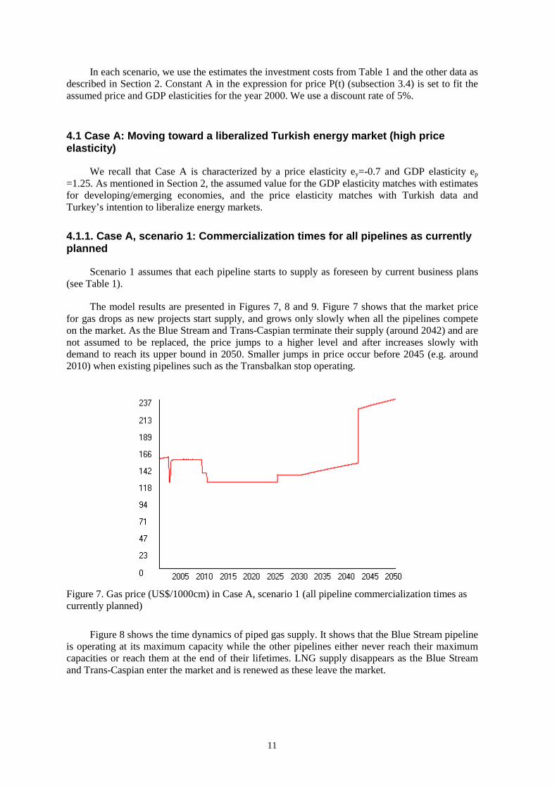
Scenario 1 assumes that each pipeline starts to supply as foreseen by current business plans (see Table 1).
The model results are presented in Figures 7, 8 and 9. Figure 7 shows that the market price for gas drops as new projects start supply, and grows only slowly when all the pipelines compete on the market. As the Blue Stream and Trans-Caspian terminate their supply (around 2042) and are not assumed to be replaced, the price jumps to a higher level and after increases slowly with demand to reach its upper bound in 2050. Smaller jumps in price occur before 2045 (e.g. around 2010) when existing pipelines such as the Transbalkan stop operating.
Figure 7. Gas price (US$/1000cm) in Case A, scenario 1 (all pipeline commercialization times as currently planned)
Figure 8 shows the time dynamics of piped gas supply. It shows that the Blue Stream pipeline is operating at its maximum capacity while the other pipelines either never reach their maximum capacities or reach them at the end of their lifetimes. LNG supply disappears as the Blue Stream and Trans-Caspian enter the market and is renewed as these leave the market.

12
Figure 8. Gas supply (bcm/year) in Case A, scenario 1 (all pipeline commercialization times as currently planned)
Figure 9 shows profits per year. Due to a high level of investment costs for the Blue Stream pipeline, profits are initially negative. Therefore, Blue Stream returns its investments later than the Trans-Caspian pipeline. The Iranpipe looks much better than Ekarum but is less competitive than the two other projects, and starts to be profitable only after the termination of Blue Stream and Trans-Caspian.
Figure 9. Profits (million US$/year) in Case A, scenario 1 (all pipeline commercialization times as currently planned)
Trans-Balkan
Iranpipe
Ekarum Blue Stream
Transcaspian LNG
Trans-Balkan
Iranpipe
Ekarum
Blue Stream
Transcaspian

13
4.1.2. Case A, scenario 2: Blue Stream’s commercialization time optimized. Other pipelines as planned
Scenario 2 assumes that the Blue Stream pipeline optimizes its commercialization time, assuming that the other pipelines will start to supply according to their current plans. The optimal commercialization time for Blue Stream is chosen so as to maximize its total profits at the end of its lifetime period.
Simulations under scenario 2 show that the optimal commercialization time for Blue Stream will be around 2005, 3 years later than planned. The rationality of this delay is explained by the fact that, as Figure 10 (a) shows, that in this case Blue Stream can start with a higher initial level of supply than in 2002 due to a higher GDP level (and hence gas demand) of Turkey. As in scenario 1, the Blue Stream reaches its maximum capacity in 2030 but maintains this level during a longer period. Moreover, in scenario 2 Blue Stream’s cost for construction is lower than in scenario 1. As a result, as seen in Figure 10 (b), in scenario 2 Blue Stream’s final profit around 2050 is about 20% higher than in scenario 1.
0
3
6
9
12
15
2000 2010 2020 2030 2040 2050
Years
Sup
ply
(bcm
/yea
r)
-4500
-3500
-2500
-1500
-500
500
1500
2500
3500
4500
2000 2010 2020 2030 2040 2050
Years
Pro
fits
(mln
US
$)
(a) Blue Stream’s gas supply (b) Blue Stream’s profit
Figure 10. Case A, scenario 1 (all pipeline commercialization times as currently planned) and scenario 2 (Blue Stream’s commercialization time optimized. Others as planned)
4.1.3. Case A, scenario 3: Trans-Caspian’s commercialization time optimized. Other pipelines as planned
Scenario 3 assumes that the Trans-Caspian optimizes its commercialization time, whereas all the other projects fix their commercialization times as planned. The optimal commercialization time for the Trans-Caspian is chosen so as to maximize its total profit at the end of its lifetime period.
Numerical results for scenario 3 show that the optimal commercialization time for the Trans-Caspian pipeline is around 2010, which is 8 years later than planned. If the Trans-Caspian starts gas supply at this optimal time, it reaches its maximum capacity in 2045 and keeps it for 5 years (see Figure 11 (a)). Total supply is increased and construction costs reduced, resulting in a total profit for the Trans-Caspian pipeline that is about 40% higher if supply starts in 2010 rather than 2002 (Figure 11 (b)).
optimized
as planned

14
0
5
10
15
20
25
30
2000 2010 2020 2030 2040 2050
Years
Sup
ply
(bcm
/yea
r))
-3100
-2100
-1100
-100
900
1900
2900
3900
4900
2000 2010 2020 2030 2040 2050
Years
Pro
fits
(mln
US
$)
(a) Trans-Caspian’s gas supply (b) Trans-Caspian’s profit
Figure 11. Case A, scenarios 1 (all pipeline commercialization times as currently planned) and 3 (Trans-Caspian’s commercialization time optimized. Others as planned)
4.1.4. Case A, scenario 4: Iranpipe’s commercialization time optimized. Other pipelines as planned
Scenario 4 assumes that the Iranpipe optimizes its commercialization time so as to maximize its total profit, whereas all the other projects stick to their currently planned commercialization times. Numerical results for scenario 4 show that the optimal commercialization time for Iranpipe is around 2010, which agrees with its current plan (see Case A, scenario 1).
4.1.5. Case A, scenario 5: Nash equilibrium in a game between the pipelines
Scenario 5 assumes that the projects’ commercialization times constitute a Nash equilibrium in a game between the pipeline projects. In this game (see Klaassen, et al., 2001) the pipeline projects act as players, projects’ commercialization times are identified with players’ strategies and the payoffs to the players are given by the total profits for the corresponding projects. The equilibrium presented here was found numerically using an iterative best response procedure.
The procedure is organized as follows. The entire time interval is split into short subintervals. The starting point is the currently planned commercialization times of the players. During the first time subinterval, the commercialization time for player 1 is optimized so as to maximize the player’s total profit, whereas the commercialization times for the other players are not changed. During the second time subinterval, the commercialization time for player 2 is optimized, whereas those for the other players are not changed. This algorithm is repeated step by step, each time a commercialization time for one player being optimized. If the players’ commercialization times eventually converge, their limits are viewed as an approximation to a Nash equilibrium in the game. The numerical experiment with the IGOR software showed good convergence. The Nash equilibrium set of projects’ commercialization times is shown in Figure 12. Table 3 gives the equilibrium times to start gas supply:
optimized
as planned

15
Table 3. Optimal commercialization times in the Nash equilibrium.
Blue Stream Trans-Caspian Ekarum Iranpipe 2003-2004 2010 2025 2010
Figure 12 shows that the Nash equilibrium (scenario 5) as compared to scenario 1 (all commercialization times as currently planned), implies that it is optimal to delay building the Blue Stream by 1-2 years, the Trans-Caspian by 8 years, and the Ekarum pipeline by 16 years. This is so since profits would be higher if these delays are implemented because investment costs would be lower and gas demand and revenues higher. The Iranpipe would still proceed as currently planned (start in 2010).
0
3
6
9
12
15
2000 2010 2020 2030 2040 2050
Years
Sup
ply
(bcm
/yea
r)
-4500
-3500
-2500
-1500
-500
500
1500
2500
3500
4500
5500
2000 2010 2020 2030 2040 2050
Years
Pro
fits
(mln
US
$)
(a) Gas supply for Blue Stream (b) Profit for Blue Stream
0
5
10
15
20
25
30
2000 2010 2020 2030 2040 2050
Years
Sup
ply
(bcm
/yea
r)
-3100
-2100
-1100
-100
900
1900
2900
3900
4900
2000 2010 2020 2030 2040 2050
Years
Pro
fits
(mln
US
$)
(c) Gas supply for Trans-Caspian (d) Profit for Trans-Caspian
0
5
10
15
20
25
30
2000 2010 2020 2030 2040 2050
Years
Sup
ply
(bcm
/yea
r))
-1450
-450
550
1550
2000 2010 2020 2030 2040 2050
Years
Pro
fits
(mln
US
$)
(e) Gas supply for Ekarum (f) Profit for Ekarum

16
0
5
10
15
20
25
30
2000 2010 2020 2030 2040 2050
Years
Sup
ply
(bcm
/yea
r)
-1300
-300
700
1700
2700
3700
4700
2000 2010 2020 2030 2040 2050
Years
Pro
fits
(mln
US
$)
(g) Gas supply for Iranpipe (h) Profit for Iranpipe
Figure 12. Case A, scenarios 1 (all pipeline commercialization times as currently planned) and 5 (Nash equilibrium)
4.2. Case B: Parameters as in typical emerging gas markets (lower price elasticity)
Case B is characterized by a lower price elasticity of ey=-0.3 and a GDP elasticity ep =1.25. These values are in line with the evidence for emerging gas markets (Komiyama, 2000).
4.2.1 Case B, scenario 1: Commercialization times for all pipelines as currently planned
In case B where the price elasticity of demand is relatively small (-0.3 instead of -0.7), the increase of supply and reduction of the price for gas cannot raise demand substantially. Thus, in this case restricting supply and holding the price at a high level can increase profits for each of the projects. Therefore, our calculations show that in scenario 1 the price for gas practically coincides with the price for LNG (Figure 13).
Nash equilibrium
As planned

17
0
50
100
150
200
250
2000 2010 2020 2030 2040 2050
Years
Pric
e (m
ln U
S$/
bcm
)
Figure 13. Gas price in Case B, scenario 1 (all commercialization times for all pipelines as currently planned)
In this case, the pipelines share a less abundant market practically uniformly (Figure 14).
Figure 14. Gas supply (bcm/year) in Case B, scenario 1 (all pipeline commercialization times as currently planned)
Figure 15 shows the time dynamics of the pipeline’s profits.
Trans-Balkan
Iranpipe
Ekarum
Blue Stream Transcaspian
LNG
Price for LNG
Price for gas
18
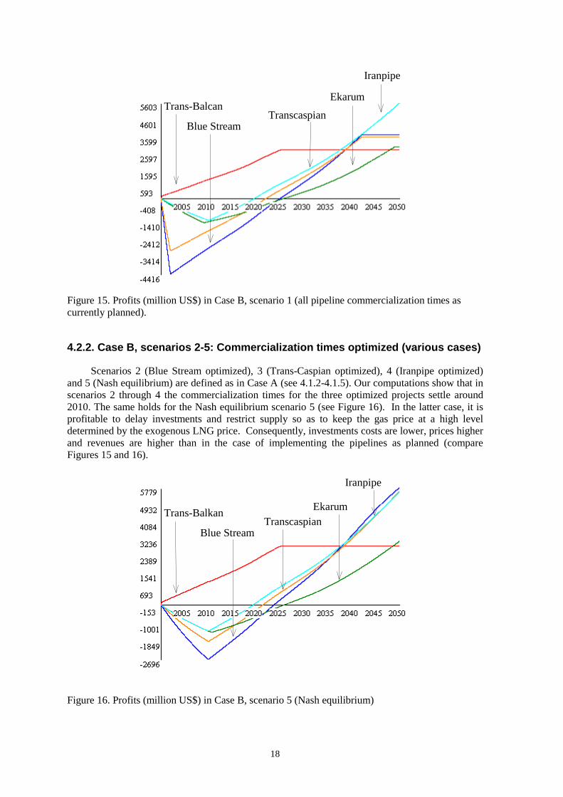
Figure 15. Profits (million US$) in Case B, scenario 1 (all pipeline commercialization times as currently planned).
4.2.2. Case B, scenarios 2-5: Commercialization times optimized (various cases)
Scenarios 2 (Blue Stream optimized), 3 (Trans-Caspian optimized), 4 (Iranpipe optimized) and 5 (Nash equilibrium) are defined as in Case A (see 4.1.2-4.1.5). Our computations show that in scenarios 2 through 4 the commercialization times for the three optimized projects settle around 2010. The same holds for the Nash equilibrium scenario 5 (see Figure 16). In the latter case, it is profitable to delay investments and restrict supply so as to keep the gas price at a high level determined by the exogenous LNG price. Consequently, investments costs are lower, prices higher and revenues are higher than in the case of implementing the pipelines as planned (compare Figures 15 and 16).
Figure 16. Profits (million US$) in Case B, scenario 5 (Nash equilibrium)
Trans-Balcan
Iranpipe
Ekarum
Blue Stream Transcaspian
Trans-Balkan
Iranpipe
Ekarum
Blue Stream Transcaspian

19
5. Sensitivity analyses
The numerical sensitivity analyses presented in this section analyze how variations in discount rate, GDP elasticity of demand and price elasticity of demand influence the performance of the proposed pipeline projects. Table 4 lists the respective reference values for these parameters.
Table 4. Reference values for the sensitivity parameters
Parameter Value
λ discount rate coefficient 0.05
ey GDP elasticity of demand 1.25
ep price elasticity of demand 0.7
We restrict our analysis to scenarios 1 and 5 (see Table 2, page 17). Let us remind that scenario 1 assumes that the pipelines’ commercialization times are chosen as currently planned and scenario 5 assumes that the pipelines’ commercialization times constitute a Nash equilibrium in the game described in subsection 4.1.5. For each experiment, we indicate those model’s outputs that are most sensitive to variations of the parameter under consideration.
5.1. Sensitivity for the GDP elasticity of demand, scenario 1 (all commercialization times as currently planned)
In this numerical experiment we fix all the model’s parameters at their reference values (Case A, scenario 1) and vary the GDP elasticity of demand, ey, from the reference value, 1.25, to 3 (the maximum value observed in the literature (Komiyama, 2000)). Figure 17 displays the years when the pipelines reach their maximum capacities as functions of ey. These functions decrease monotonically, which shows that the higher the GDP elasticity, the shorter the projects’ saturation periods. As an explanation, we may recall that a higher GDP elasticity implies a higher increase in gas demand as the GDP grows. In turn, a higher demand implies higher supply with no essential changes in price. Hence, growth in the GDP elasticity results in shortening the saturation periods of the pipelines.
As the GDP elasticity, ey, ranges from 1.25 to 3 the saturation period for each project shrinks by around 10 years, which shows its high sensitivity with respect to ey.

20
2010
2020
2030
2040
2050
1.25 1.5 1.75 2 2.25 2.5 2.75 3
GDP elasticity, ey
Yea
rs Blue Stream
Trans-Caspian
Ekarum
Iranpipe
Figure 17. Years of saturation in Case A, scenario 1
Figure 18 depicts profits in the year 2050 as functions of ey. These functions are monotonically increasing, which shows that profits are positively related to the GDP elasticity. An explanation is that, as noted earlier, growth in ey implies growth in supply. Figure 18 shows that projects with higher capacities are more sensitive to variations in ey.
-1000
1000
3000
5000
7000
9000
11000
13000
15000
1.25 1.5 1.75 2 2.25 2.5 2.75 3
GDP elasticity, ey
Pro
fits
(m
ln U
S$)
Blue Stream
Trans-Caspian
Ekarum
Iranpipe
Figure 18. Projects’ profits in 2050 for Case A, scenario 1
5.2. Sensitivity of the results for the price elasticity of demand, scenario 1 (all commercialization times as currently planned)
In the next experiment, we vary the price elasticity of demand, ep, from -0.3 to the reference value, -0.7. All other parameters are fixed at their reference values. Figure 19 presents price for gas in the year 2020 as a function of ep. This function decreases, which can be explained as follows. If the price elasticity, ep, is low, price has little influence on demand. Hence, the projects do not compete actively, but withhold new pipeline capacity to keep the price at a high level. As a result, the price for gas follows its upper bound, the price for LNG. As price elasticity grows, the projects start to compete and the price for gas drops.

21
0
50
100
150
200
250
0.3 0.35 0.4 0.45 0.5 0.55 0.6 0.65 0.7
Price elasticity, ep
Pri
ce (
mln
US
$/b
cm)
Figure 19. Price for gas in 2020 in Case A, scenario 1
Figure 20 presents profits in the year 2050 as functions of the price elasticity of demand, ep. We see that for small ep the profits grow together with ep. Starting from a certain critical ep (around 0.45) profits decrease as ep continues to grow. To explain this phenomenon, we can address the fact that, generally, the increase in the price elasticity implies an increase in supply. Hence, if the market competition is not clearly seen (which, as noted above, corresponds to low enough ep) the increase in ep enlarges profits due to the increase in supply. The critical value of ep can be viewed as a saturation point, at which price and supply reach their highest limits and competition between the projects not only decreases the price while increasing supply but also lowers the net profits. Figure 20 shows that the profitability of Blue Stream becomes higher as the price elasticity, ep, grows but only up to a level of 0.45.
0
2000
4000
6000
8000
10000
12000
14000
0.3 0.35 0.4 0.45 0.5 0.55 0.6 0.65 0.7
Price elasticity, ep
Pro
fits
(m
ln U
S$)
Blue Stream
Trans-Caspian
Ekarum
Iranpipe
Figure 20. Project's profits in 2050 for Case A, scenario 1
5.3. Sensitivity of the results for changes in the discount rate, scenario 1 (all commercialization times as currently planned)
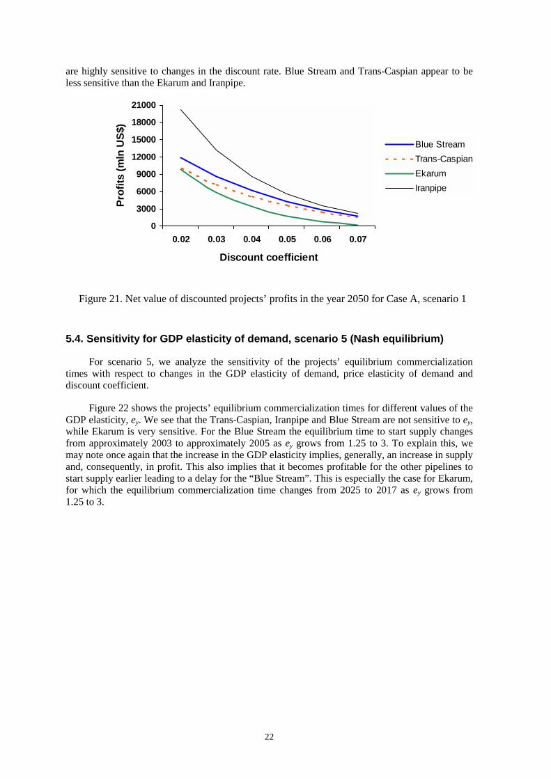
In the next numerical experiment, we fix all the model’s parameters at their reference values (Case A, scenario 1) and vary the discount rate, λ, from 0.02 to 0.07. Figure 21 presents profits in the year 2050 as functions of λ. These functions are rapidly decreasing, which shows that profits
22
are highly sensitive to changes in the discount rate. Blue Stream and Trans-Caspian appear to be less sensitive than the Ekarum and Iranpipe.
0
3000
6000
9000
12000
15000
18000
21000
0.02 0.03 0.04 0.05 0.06 0.07
Discount coefficient
Pro
fits
(m
ln U
S$)
Blue Stream
Trans-Caspian
Ekarum
Iranpipe
Figure 21. Net value of discounted projects’ profits in the year 2050 for Case A, scenario 1
5.4. Sensitivity for GDP elasticity of demand, scenario 5 (Nash equilibrium)
For scenario 5, we analyze the sensitivity of the projects’ equilibrium commercialization times with respect to changes in the GDP elasticity of demand, price elasticity of demand and discount coefficient.
Figure 22 shows the projects’ equilibrium commercialization times for different values of the GDP elasticity, ey. We see that the Trans-Caspian, Iranpipe and Blue Stream are not sensitive to ey, while Ekarum is very sensitive. For the Blue Stream the equilibrium time to start supply changes from approximately 2003 to approximately 2005 as ey grows from 1.25 to 3. To explain this, we may note once again that the increase in the GDP elasticity implies, generally, an increase in supply and, consequently, in profit. This also implies that it becomes profitable for the other pipelines to start supply earlier leading to a delay for the “Blue Stream”. This is especially the case for Ekarum, for which the equilibrium commercialization time changes from 2025 to 2017 as ey grows from 1.25 to 3.

23
2000
2005
2010
2015
2020
2025
Yea
rs
1.25
1.50
1.75
2.00
2.25
2.50
2.75
3.00
GDP elasticity, e y
Blue Stream
Trans-Caspian
Ekarum
Iranpipe
Figure 22. Sensitivity of commercialization times in Case A, scenario 5 (Nash equilibrium)
5.5. Sensitivity for price elasticity of demand, scenario 5 (Nash equilibrium)
Figure 23 presents the projects’ equilibrium commercialization times as functions of the price elasticity, ep. As ep approaches its lower bound, -0.3, the equilibrium commercialization times concentrate around 2009, and they differ significantly (see the right hand side of Figure 23) when ep approaches its upper bound, -0.7. To explain this phenomenon, we may argue as follows. If the price elasticity is relatively low, the projects can share the market more or less equally; hence, under the equilibrium scenario, they commercialize simultaneously, at a later time (so as to reduce the construction costs), and supply gas at a high price. At higher values of the price elasticity competition becomes more intense and this cooperative commercialization strategy of sharing the market does no longer lead to an equilibrium. For the Blue Stream it becomes profitable to start supply earlier and for Ekarum later. It is remarkable that for the Trans-Caspian and Iranpipe the equilibrium commercialization times are quite insensitive to variations in ep.

24
Figure 23. Sensitivity of commercialization times in Case A, scenario 5 (Nash equilibrium).
5.6. Sensitivity for the discount rate, scenario 5 (Nash equilibrium)
Figure 24 shows the projects’ equilibrium commercialization times computed for different values of the discount rate, λ. We see that as λ increases, the equilibrium commercialization times tend to decrease for the Blue Stream and Trans-Caspian but tend to increase for the Ekarum pipeline. Only for a very high discount rate (0.15) commercialization of the Blue Stream would be delayed until 2030 and the Trans-Caspian would be built already in 2005. This is due to the high initial investments of the Blue Stream.
Figure 24. Sensitivity of commercialization times for Case A, scenario 5 (Nash equilibrium).
2000
2005
2010
2015
2020
2025
Yea
rs
0.30 0.40 0.50 0.60 0.70
Price elasticity, e p
Blue Stream
Trans-Caspian
Ekarum
Iranpipe
2000
2005
2010
2015
2020
2025
2030
Yea
rs
0.02 0.04 0.06 0.15
Discount coefficient
Blue Stream
Trans-Caspian
Ekarum
Iranpipe

25
6. Conclusions
We have presented results of a numerical analysis of the international gas pipeline routings to the Turkey market, including comprehensive sensitivity analyses. For this purpose, a new economic model of the performance of international gas pipeline projects has been recently developed by IIASA’s DYN/ECS projects. The model was based on the new DYN-elaborated IGOR software package and ECS data for the Turkey gas market.
Assuming a future move toward a liberalized Turkish energy market (i.e., assuming a high price elasticity of -0.7), the (optimal) Nash equilibrium solution implies that the “Blue Stream” pipeline project would start gas supply by 2003/2004, the “Trans-Caspian” pipeline by 2010 and the “Iranpipe” by 2010. However, assuming no significant liberalization, i.e., assuming a lower price elasticity (-0.3), all optimal pipeline commercialization times are delayed until 2010. The optimal commercialization time of the “Blue Stream” pipeline is very sensitive to the price elasticity and discount rate and less sensitive to the assumed GDP elasticity. The optimal timing of the “Trans-Caspian” pipeline is rather insensitive to all three factors. The “Iranpipe” pipeline is more sensitive to the discount rate. The “Ekarum” pipeline, being the least profitable of all four new pipeline projects, is very sensitive to all three factors.
For investors our central case with a high gas price elasticity and moderate GDP elasticity of gas demand shows that the Blue stream pipeline should indeed (as is the case in reality) be the first one to be built. Commercialization of the Transcaspian pipeline and the pipeline from Iran is only viable financially around 2010. This result holds for different GDP elasticities. Only when the price elasticity is lower than –0.5 commercialization of the Blue stream should be delayed beyond 2005. The same applies when the interest rate would be 15%. Building the Blue stream seems to be a robust first choice. If the other investors want to maximize profits commercialization of their pipelines may have to wait until the year 2010.
Future research should address more directly the issues of economic and political risks. The current model structure is ideal to include these risk factors. An extension of the model could address the possibility of substitution between gas and other fuels (oil, coal, renewables etc.), possibly by linking IGOR to available energy models. Finally, the model could be applied to other regions or a multimarket/multiregional version of the model could be made to address interactions between different markets in Eurasia.

26
Appendix
This Section describes the software package IGOR that was used to match the model described in section 3 with the data on the Turkish market. The IGOR package includes an input interface, several computing modules and an output module that simulates a gas market for user-defined input data and displays various output parameters in a user-friendly way. Table A shows the basic inputs and outputs for IGOR.
Table A. Inputs and outputs for IGOR
Inputs Outputs Initial time, T0
Price for gas, P
Final time, TEND
Step, DELT
STATE OF PIPELINE I
Number of pipelines, N
Initial price for gas, P0
Accumulated investment, X[I]
Current investment, U[I] STATE OF ENVIRONMENT Current supply, Y[I]
Accumulated supply, YY[I] Gross Domestic Product, GDP Commercialization level, CL[I]
Upper reference price of gas, PLNG Profit, B[I] Discount coefficient, λ Obsolescence coefficient, σ Discount return coefficient, γ Price elasticity of gas demand, ep GDP elasticity of gas demand, ey
INITIAL STATE OF PIPELINE I
Initial accumulated investment, X0[I]
Initial current supply, Y0[I]
Initial accumulated supply, YY0[I]
Initial commercialization level, CL0[I]
Initial profit, B0[I]
OTHER INITIAL DATA FOR PIPELINE I
Number of capacities, K[I]
Lifetime, TL[I]
Commercialization times,
Input:
State of environment & initial data
IGOR Output:
State of pipelines

27
COMT[I,1],…,COMT[I,K[I]]
Project capacities,
PM[I,1],…,PM[I,K[I]]
Extraction costs, CE[I]
Transportation costs, CT[I]
Distribution costs, CD[I]
Transit fees, CF[I]
Figure A1 shows the basic scheme of IGOR. The next blocks compute basic outputs:
CURRENT INVESTMENT realizes scenarios to compute current investment for a pipeline;
CURRENT SUPPLY computes current supply for a pipeline;
ACCUMULATED INVESTMENT (SUPPLY) computes accumulated investment (supply) for a pipeline;
ENVIRONMENT GENERATOR defines current parameters of the environment;
COST GENERATOR defines current costs of extraction, transportation costs, distribution costs and transit fees for a pipeline.

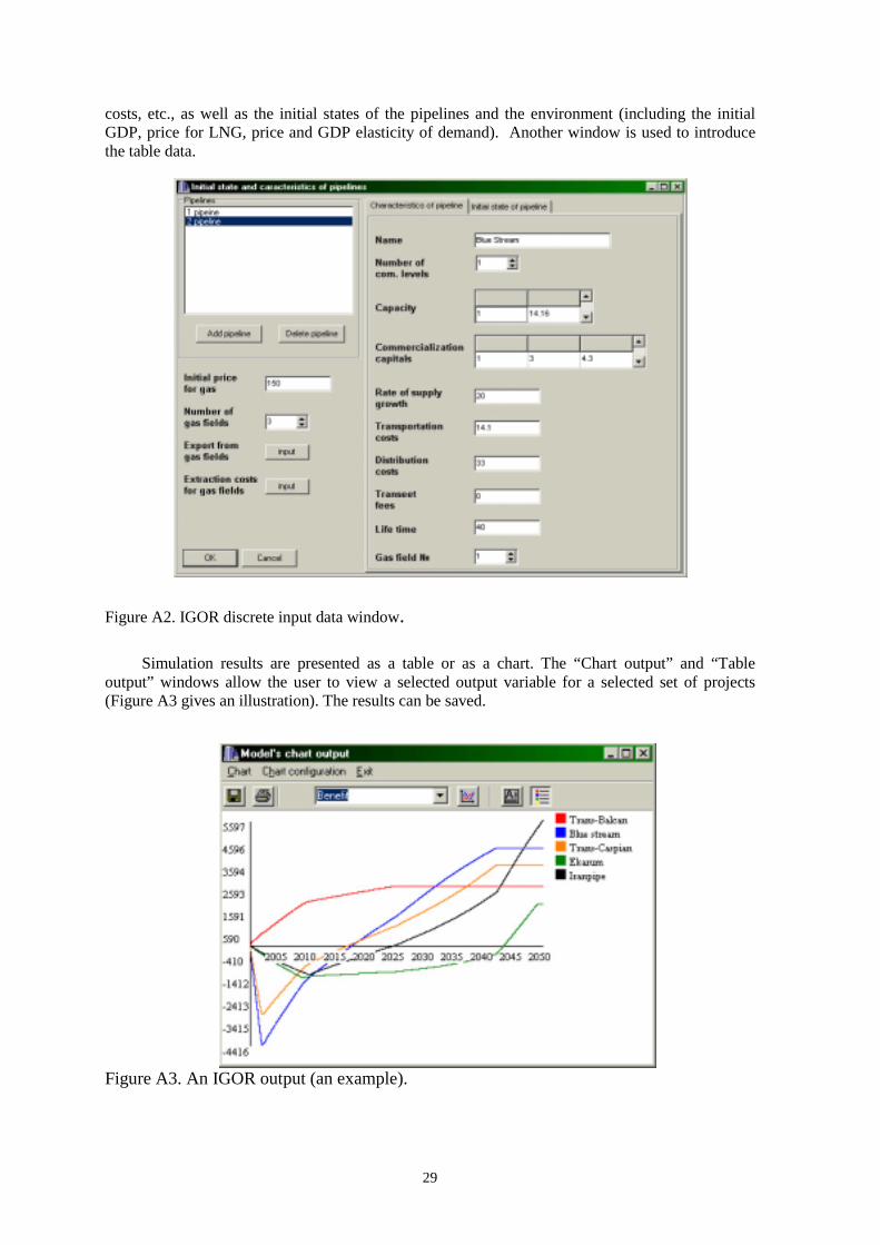
28
Figure A2 shows the IGOR discrete data input window, using which the user introduces discrete input parameters such as the number of commercialization levels, maximum capacities,
IGOR
INPUT DATA
ENVIRONMENT
GENERATOR (define state of
COST GENERATOR (define costs for
T=T0+DEL
Calculation of price, P
CL[I]=K[I
I=1
CURRENT INVESTMENT
ACCUMULATED
CL[I]=0
CURRENT SUPPLY
ACCUMULATED SUPPLY
PROFIT (B[I])
COM. LEVEL (define
commercialization level of
pipeline, CL[I],
T≤TEND
I≤N
OUTPUT DATA
NO
NO
NO
NO
YES
YES
T=T0+DEL
I=I+1
YES
YES
Figure A1. Block-scheme of IGOR
29
costs, etc., as well as the initial states of the pipelines and the environment (including the initial GDP, price for LNG, price and GDP elasticity of demand). Another window is used to introduce the table data.
Figure A2. IGOR discrete input data window.
Simulation results are presented as a table or as a chart. The “Chart output” and “Table output” windows allow the user to view a selected output variable for a selected set of projects (Figure A3 gives an illustration). The results can be saved.
Figure A3. An IGOR output (an example).

30
References
Anonymous, 2002, Russia: first of two lines of the “Blue stream” gas pipelines has been completed, Inzheneraia Gazeta, February 26, 2002, page 3.
EIA, 1999a, Turkey, August 1999, United States Energy Information Administration, Washington, www.eia.doe.gov/emeu/cabs/turkey.html.
EIA, 1999b, Caspian Sea Region, December 1998, United States Energy Information Administration, Washington.
www.eia.doe.gov/emeu/cabs/caspfull.html.
EIA, 2001, Turkey, July 2000, United States Energy Information Administration, Washington, www.eia.doe.gov/emeu/cabs/turkey.html.
Golombek, R., Gfelsvik, E., Rosendahl, K.E., 1995, Effects of liberalizing the natural gas markets in Western Europe, The Energy Journal, 16, No 1, 85-111.
Ignatius, D., 2000, The great game gets rough, The Washington Post, January 26, A23.
Klaassen, G., Kryazhimskii, A.V., and Tarasyev, A.M., 2001, Competition of gas pipeline projects: a game of timing, International Institute for Applied Systems Analysis, Laxenburg, Austria, Interim Report IR-01-037.
Komiyama, R., 2000, Projecting long-term natural gas demand as a function of price and income elasticities, IIASA, Laxenburg, draft unpublished document.
Matrosov, I., 2000, Game model of investment dynamics on markets of gas pipelines, unpublished manuscript.
Nakicenovic, N., J., Alcamo, D. G., de Vries, B., Fenhann, J., et al., 2000, Special Report on Emission Scenarios (SRES), A special report of working group III of the intergovernmental panel on climate change, Cambridge University Press, Cambridge, UK.
Quinlan, M., 2002, Extreme ambitions: Turkey’s gas ambitions appear boundless, Petroleum Economist, 69 (5), p. 6.
Riahi, K., and Roehrl, A., 2000, Greenhouse gas emissions in a dynamics-as-usual scenario of economic and energy development, Technological Forecasting and Social Change, 63, 175-205.
Roehrl, R.A., Klaassen, G., and Tarasyev, A., 2000, The great Caspian gas pipeline game, Risk Management: Modeling and Computer Applications, Proceedings of IIASA Workshop, May 14-15, 2001 (V.Maksimov, Yu.Ermoliev, and J.Linnerooth-Bayer, eds.), International Institute for Applied Systems Analysis, Laxenburg, Austria, Interim Report IR-01-066, 107-131.
Rogner, H.-H., 1997, An assessment of world hydrocarbon resources, Annual Review of Energy and Environment, 22:217-262, 1997.
Sagers, M., 1999, Turkmenistan's gas trade: the case of exports to Ukraine, Post-Soviet Geography and Economics, 40, No 2, 142-149.
Strubegger, M., and Messner, S., 1995, User guide of Message III, International Institute for Applied Systems Analysis, Laxenburg, Austria, Working Paper WP-95-069.
Zhao, J., 2000, Diffusion, costs and learning in the development of international gas transmission lines, International Institute for Applied Systems Analysis, Laxenburg, Austria, Interim Report IR-00-054.