Intergenerational Mobility in Educational Attainments

© The Pakistan Development Review

59:2 (2020) pp. 179–198 DOI: 10.30541/v59i2pp.179-198

Intergenerational Mobility in

Educational Attainments

MALIK MUHAMMAD and MUHAMMAD JAMIL*

This paper investigates intergenerational educational mobility, a non-monetary measure

of socioeconomic status in Pakistan. Data from the Pakistan Social and Living Standards

Measurements (PSLM-2012-13) are used for empirical analysis. Contingency tables and

multinomial logit model are utilised. Results indicate strong evidence of intergenerational

linkages in educational attainments between fathers and their sons. Although findings reveal

some degree of upward mobility, opportunities are not equal for all. Chances for attainment of

higher education for sons of fathers with education up to the secondary level only, are not as

prevalent as for sons of highly educated fathers. Further, urban areas show higher mobility as

compared to rural areas. Results also reveal that the affluent are more likely to attain higher

levels of education than the financially disadvantaged. In addition, sons of affluent families in

rural areas are less likely to attain higher levels of education compared to the sons of the

affluent in urban areas. Our findings also support evidence in favour of the child quality-

quantity trade-off as shown by negative impacts of family size on attainment of higher levels

of education.

JEL Classification: C24, J24, L86, O43, O47

Keywords: Inequality of Opportunity, Education, Intergenerational Mobility

1. INTRODUCTION

Intergenerational mobility in socioeconomic status is the link between the

socioeconomic status of parents and their children as adults. If this link is strong, there

will be more persistence in society. On the other hand, a society is termed more mobile if

the link between the socioeconomic status of parents and their children is weak. Due to

various forms of discrimination, some specific social classes are excluded from the

capability formation process and income earning opportunities. As a result, both current

and future generations of these classes experience backwardness, deprivation, and

increase in inequality and poverty.

The poor are excluded from wider participation in income generating activities

because of their relatively weak financial position, while exclusion from capability

formation opportunities due to low income also renders them poorly endowed in terms of

human capital. This reduces the income of their next generation and thus the same status

persists across generations. In less mobile societies, human skills and talents are more

Malik Muhammad <[email protected]> is Assistant Professor, IIIE, International Islamic

University Islamabad. Muhammad Jamil <[email protected]> is Assistant Professor, School of Economics,

Quaid-i-Azam University, Islamabad.

mailto:[email protected]

180 Muhammad and Jamil

likely to be wasted, and talented members from poor families are likely to remain

underdeveloped. Further, lack of equal opportunity may affect the motivation and efforts

of individuals reducing the overall efficiency and growth potential of an economy.

Higher intergenerational mobility ensures placement of individuals in a society

according to their competence rather than social origin. It increases the optimal utilisation

of talented individuals, and enhances productivity and economic growth. Earnings,

occupation, and education measure the socioeconomic status of an individual.

Economists widely use income as a proxy for socioeconomic status.

Starting from contributions by Becker and Tomes (1979, 1986), and Loury (1981),

economists have increasingly paid attention to the issue of inequality in income among

families over generations and attempted to estimate intergenerational income mobility,

producing diverse results over time and across regions. We find that income suffers from

a number of problems. It is influenced by time and cycles. It is also affected by individual

and aggregated temporary shocks. Moreover, income significantly varies over a life

cycle. Patterns of income observed in a life cycle also vary from generation to generation.

Therefore, it becomes quite difficult to find a link between incomes of parents and their

children to evaluate the strength of intergenerational mobility on socioeconomic status.

However, education is less likely to be exposed to measurement errors, and

unlikely to bias estimation by life cycle bias, as most individuals complete their education

by their early or mid-twenties. The level of education reveals information about the life

of an individual. Higher levels of education are associated with higher earnings, better

health, longer lifespan and other economic outcomes (Solon et al. 1994; Blanden, 2009;

Black & Devereux, 2011). Education increases the probability of upward occupational

and income mobility. It produces mobility aspirations, socialises an individual for better

work role and position. Therefore, it is a reasonable proxy to measure the overall

socioeconomic status of individuals. Mobility of education, therefore, would mean

mobility in overall socioeconomic status.

There is ample research on intergenerational mobility at the international level but

Pakistan lacks similar in-depth study in this area. Social exclusion, income inequality,

poverty, and low economic growth are quite prevalent in Pakistan. So far, researchers

have focused on a particular “outcome” variable (e.g. earning, consumption, expenditure,

or wealth) and determined how inequality in this variable has changed over time.

However, in the context of Pakistan, no researcher has focused comprehensively on

intergenerational mobility, addressing the extent to which the outcomes for the present

generation influences the previous generations’ characteristics.

In this paper, we try to fill the void in existing literature by exploring not only the

level of educational attainment in Pakistan but also the degree of educational mobility.

We also extend our analysis to urban and rural areas separately. We utilise the most

comprehensive and representative data of Pakistan Social and Living Standards

Measurements (PSLM-2012-13) which covers almost all the districts.

2. SIGNIFICANCE AND OBJECTIVES OF THE STUDY

Enhancing economic growth, and reducing inequality and poverty, are the main

concerns of policy-makers throughout the world, as well as in Pakistan. Pakistan’s

growth rate remained below other countries in the region. It also has a lower per capita

Intergenerational Mobility in Educational Attainments 181

income, high multidimensional poverty, and a low quality of human capital.1 The average

years of schooling are 4.7 years only, ranking Pakistan 150th in the world. Inequality in

education is 44.4 percent, much higher than the global average of 26.8 percent. Pakistan

spends 2.5 percent of GDP2 on education, which makes it amongst the lowest in the

world, ranking 147th out of 188 countries.

Most researchers and policy-makers focus at the macro dimensions of these

indicators. For example, what are the determinants of economic growth and inequality?

Which factors are most and least important? There seems to be little research available

regarding inequality in opportunity via educational mobility in Pakistan. There is an

increasing role of human capital in economic growth, which in turn affects fertility and

mortality (Meltzer, 1992). Decisions about fertility and education depend on constraints

faced by parents, as well as their preferences. This provides a strong basis for the role of

family in the transmission of human capital in theories of intergenerational mobility.

In this study, our focus is on intergenerational mobility in educational attainments

with reference to Pakistan. Due to the nature of available data, our analysis is limited to

co-resident father-son only. Most females leave the parents’ home after marriage so

limited observations are available, especially for those over 25 years of age. Moreover,

the number of educated females, especially those obtaining higher education, is very low.

Of co-resident mothers, 83.36 percent never attended school. For these reasons, our

analysis is limited to intergenerational mobility in educational attainments of co-resident

father-son data only. Specific objectives of the study are:

To examine structure of educational attainments in both fathers and sons

generations.

To investigate intergenerational mobility at the secondary and higher levels of

education.

To examine the differences in intergenerational mobility in education across

urban and rural areas.

3. LITERATURE REVIEW

Intergenerational mobility is one of the most studied topics in social sciences. The

first study dates back to Galton (1886), a biologist, who regressed heights of children on

the heights of their parents. Leading economists started to evaluate income mobility in

the latter half of the 20th century. Pioneering studies can be attributed to Soltow (1965),

and Wolff and Slijpe (1973) for Scandinavia, and Sewell and Hauser (1975) for US.

However, economists developed an interest in this topic after Becker and Tomes (1979,

1986) formally developed a model of the transmission of education, earnings, assets and

consumptions from parents to children. Much research is available on the positive

relationship between the level of education of parents and their children.

Mare (1980) shows that the impact of parental education and income declines as

the child progresses to higher education. Lillard and Wallis (1994) found that educational

effects moved along gender lines in Malaysia where a mother’s education had a strong

effect on her daughter’s education, and a father’s education had a relatively higher impact

1 Ranked as 147th out of 188 countries with HDI value of 0.538 (UNDP-2015). 2 This figure is for year 2014.


on his son’s educational level. However, in general, for educational attainments of

children, a father’s education is more important as compared to their mother’s. Burns

(2001) shows that a child with a poorly educated mother and a highly educated father has

the same schooling outcomes as having two well-educated parents.

Spielaure (2004) observes higher mobility at higher levels of education for

Australia, which varies across regions and gender. Hertz et al. (2007) observe significant

regional differences in educational mobility in a sample of 42 countries with Latin

America being the lowest and the Nordic countries the highest. In Switzerland, Bauer and

Riphahn (2009) show a positive impact of early enrolment on educational mobility,

which, according to authors, is because once children are in school, inequalities in family

background have a lesser impact on their education.

Van Doorn et al. (2011) found that industrialisation, female participation in the job

market, and increase in educational expenditure positively influences intergenerational

educational mobility. In China, apart from parental education, Labar (2011) finds a

significantly positive affect of income, and being located in an urban area, on education

of a child. Parental characteristics increase in importance at a higher level of education.

In India, Azam and Bhatt (2015) find upward mobility in educational attainments

and show that mobility has a strong association with the per capita spending on education

at the state level. Moreover, Assad and Saleh (2016) show a significant impact of public

school supply on intergenerational mobility in education in Jordan. The study also finds

that daughters are more mobile compared to sons, especially in the current cohorts.

Nguyen and Getinet (2003) show that in the U.S. an increase in the number of children in

a family dilutes the resources of parents and thus reduces educational mobility.

Researchers studying this topic for Pakistan include Havinga et al. (1986), Cheema

and Naseer (2013), and Javed and Irfan (2014). Havinga et al. (1986), in a sample from

10 major industrialised cities, finds that 31 percent of the sons have a higher income than

their fathers, with 60 percent of the sons owning more wealth than their fathers did. For

rural Sargodha, Cheema and Naseer (2013) show an increase in intergenerational

mobility in education as grandfather-father pairs show more rigidity than father-son pairs.

Their results also indicate that mobility in non-propertied groups is less than in propertied

groups, and is much higher among zamindar(landlords) than in artisan and historically

depressed quoms (sects).

Using data from the Pakistan Panel Household Survey (2010), Javed and Irfan

(2014) show a strong persistence in educational attainments. Particularly, this persistence

is higher in older cohorts as compared to younger cohorts. They also find more

persistence in low status occupations and downward mobility in high status occupations.

Further, a higher persistence at the lowest income quintile is evident. Regression results

of their study suggest that income mobility in urban areas is higher than in rural areas,

with older cohorts being more mobile than younger cohorts are.

4. THEORETICAL FRAMEWORK

We utilise models developed by Becker and Tomes (1979), and Becker et al.

(2015), in which parents are assumed to be altruistic. They not only care about their own

utility, but also care about the “quality” and “economic success” of their children in the

form of income as given by the following utility function:


𝑉(𝑌𝑃) = 𝑢(𝑐) + 𝛼𝐸𝑣(𝑌𝑐ℎ) … … … … … … (1)

Where 𝑌𝑃 and 𝑉(𝑌𝑃) are income and total utility of parents respectively, 𝑢(𝑐) is the

utility that parent derive from consumption (𝑐), 𝛼 is the degree of altruism which ranges

from 0 to 1. 𝐸𝑣(𝑌𝑐ℎ) is the expected utility a child derives from income (𝑌𝑐ℎ) in future.

Let 𝑌𝐻 is the amount invested in the human capital formation (education) of a child by

parent and 𝜏 is the cost of consumption forgone against each unit of 𝑌𝐻 , then budget

constraint of parents can be written as

𝐶 + 𝜏𝑌𝐻 = 𝑌𝑃 … … … … … … … (2)

By assuming that value of each unit of human capital accumulated in children is

equal to 𝑤1, the present value of this investment can be expressed as:

𝜏𝑌𝐻 =𝑤1𝑌𝐻

1+𝑟 … … … … … … … (3)

Total income of a child is equal to the sum of income earned from “human capital

(𝑌𝐻)”, “endowed capital (𝐾)” and “labour market luck (𝑔)” (Becker and Tomes, 1979)

and can be expressed by the following equation:

𝑌𝑐ℎ = 𝑤1𝑌𝐻 + 𝑤2𝐾 + 𝑤3𝑔 … … … … … … (4)

Putting Equations (4) and (3) into Equation (2), we get the budget constraint

𝐶 +𝑌𝑐ℎ

1+𝑟= 𝑌𝑃 +

𝑤2𝐾

1+𝑟+

𝑤3𝑔

1+𝑟 … … … … … … (5)

Parents maximise utility (1) subject to budget constraint (5). This provides the

basis for intergenerational linkages between parental characteristics and the human

capital of children.

Parental education influences the level of education of their children through

different mechanisms:

(1) Highly educated parents generally have higher incomes, which relaxes their budget

constraints and may positively affect educational attainment of their children.

(2) Educated parents may be more efficient in child rearing activities, which

results in higher educational attainment by the child.

(3) Parents that are more educated may be more successful in directing

expenditures towards child-friendly activities and investments.

(4) Educated parents may have a greater concern for the education of their

children as compared to uneducated parents3 and are more likely to help

children with homework, being able to guide them better with their schooling.

With this background, our general model is

𝐸𝐷𝑖𝑗𝑐ℎ = 𝑓(𝐸𝐷𝑖𝑗

𝑃 , 𝑌𝑖𝑃 , X) … … … … … … (6)

where 𝐸𝐷𝑖𝑗𝑐ℎ is the j

th level of education of an i

th child, 𝐸𝐷𝑖𝑗

𝑃 is the jth

level of education of

parent of an ith

child , 𝑌𝑖𝑃 is income of the parent of an i

th child and X is the vector of

other control variables.

3Guryan et al. (2008) in their American Time Survey show that average time spent with children by

educated parents is larger than with uneducated parents.


Along with education and income of parents, some additional factors to consider:

Wealth influences education attainment of a son. More wealth in the form of

durables means that the family has already met its needs and more income is

available for the children’s education. Moreover, wealth, especially land, is

available as collateral for a loan to finance education in case parents are facing

financial constraints.

Additional children the amount of time, money, and patience that each child

receives from parents are diluted and may strain the parents’ finite resources.

Therefore, the chance for a child to achieve higher social status, for example,

through higher level of education is reduced (Downey, 1995; Maralani, 2008).

Age of a child is another factor that is a control variable. As the age of a child

increases, we expect an increase in his/her level of education.

Geographic location may be capturing, for example, availability and quality of

schools across different provinces, and across urban-rural areas. It captures peer

effects as well as the environmental effects.

With these parameters we can write Equation (6) as:

𝐸𝐷𝑖𝑗𝑐ℎ = 𝑓(𝐸𝐷𝑖𝑗

𝑃 , 𝑌𝑖𝑃 , 𝑊𝑖

𝑃 , 𝐻𝑆𝑖 , 𝐴𝑖𝑐ℎ , 𝑅𝑅, 𝑃𝑝, 𝑃𝑆,𝑃𝐵) … … … (7)

Where 𝑊𝑖𝑃 is the wealth of parent of i

th child, 𝐻𝑆𝑖 is the household size where i

th child

lives, 𝐴𝑖𝑐ℎ is the age of i

th child, 𝑅𝑅 equal to “1” if a child belongs to rural region and

equal to “0” otherwise. 𝑃𝑝 , 𝑃𝑆 and 𝑃𝐵 are dummies for provinces Punjab, Sindh and

Balochistan respectively. Province Khyber Pakhtunkhwa (KPK) is used as reference

province. In stochastic form, Equation (7) can be written as:

𝐸𝐷𝑖𝑗𝑐ℎ = 𝛽0 + 𝛽1𝐸𝐷𝑖𝑗

𝑃 + 𝛽2𝑌𝑖𝑃 + 𝛽3𝑊𝑖

𝑃 + 𝛽4𝐻𝑆𝑖 + 𝛽5𝐴𝑖𝑐ℎ + 𝛽6(𝐴𝑖

𝑐ℎ)2 + 𝛽7𝑅𝑅

+𝛽8𝑃𝑝 + 𝛽9𝑃𝑆 + 𝛽10𝑃𝐵 + 𝑒𝑖 … … … … … (8)

(𝐴𝑖𝑐ℎ)2 is the square of age of ith

child. Error term “ei” captures the effects of all other

omitted variables.

5. DATA

We utilise PSLM (2012-13) survey data, which covers urban and rural areas of all

districts of the four provinces of Pakistan. However, there are some issues and limitations

of the PSLM survey data:

(1) PSLM survey focuses on co-resident children-parents pairs only and misses

information regarding younger generations who are living out of the parents’

residence.

(2) Survey does not report information regarding the fathers of married women,

who constitute the majority of women.

(3) In our co-resident data, 84.36 percent of the mothers have never attended schools

and their frequency in the “postgraduate” category is zero. For this reason, our

analysis is restricted to co-resident father-son pairs only. We extracted

information on 39989 co-resident father-son pairs, with sons of age 16 years and

above, who have completed their education and are not currently enrolled in any


educational institution. Once we identified father-son pairs then data on relevant

variables were obtained. These variables are discussed below.

Originally, 21 categories of Levels of Education are framed, including “no education”

in the PSLM data. We drop category “other” which consists of mixed levels of education such

as short diploma, short certificate, religious education etc. The remaining 20 categories are re-

coded into 7 categories: (1) Never attended school (2) Up to Primary (3) Up to Middle (4)

Matriculation (5) Intermediate (6) Graduate (7) Post-Graduate.

Income of father is the sum of all types of income he receives from various

sources. This includes salary, wages, pension, remittances, and rent from property. We

construct a wealth index for variable wealth, which includes twenty durables,4 access to

two public utilities,5 four housing characteristics,

6 source of cooking fuel, type of phone

used for communication (land line, mobile or both), personal agricultural land, poultry,

livestock, non-agriculture land, and residential / commercial property. This set of assets is

selected due to their availability in PSLM survey. We use Principal Component Analysis

(PCA) for the construction of wealth index.

Household size means the number of individuals living in a household.

Information on household size is taken from the roster of PSLM. Age of a son is reported

in years. Region effects are captured through dummy variables. For rural-urban areas, we

introduce a dummy variable which takes value “1” if rural and “0” otherwise. For

provinces, we introduce three dummy variables for Punjab, Sindh and Balochistan. KPK

is taken as reference province.

6. RESULTS AND DISCUSSION

To understand the structure of educational attainments we compute percentage

distribution of sons and fathers falling in different levels of education. This is useful for

further analysis of educational mobility. Table 1 summarises the results.

Table 1

Percentage Distribution of Different Levels Education

Level of Education

Father Son

Pakistan Urban Rural Pakistan Urban Rural

Never Attend School 58.4 39.9 67.0 27.6 15.2 33.3

Primary 17.5 19.7 16.5 22.6 17.9 24.7

Middle 9.4 13.5 7.4 20.7 23.7 19.3

Matric 9.0 15.6 6.0 16.6 21.1 14.7

Intermediate 2.8 5.3 1.6 6.8 10.7 5.1

Graduate 1.4 2.7 0.8 3.2 6.0 1.8

Post Graduate 1.5 3.3 0.7 2.5 5.5 1.1

Average Years of Education 3.5 5.3 2.5 6.2 7.9 5.3 Source: Author’s own calculations based on PSLM (2012-13).

4 Possession of iron, fan, sewing machine, chair/table, radio or cassette player, watch, TV, VCR/

VCP/VCD, refrigerator/freezer, air cooler, air conditioner, computer/ laptop, phone or mobile, bicycle, motor

cycle, car, tractor/ truck, cooking range, stove and washing machine. 5Water and electricity. 6Number of sleeping rooms, quality of floor material, quality of wall material and toilet facility.


Percentages in the lower levels of education are higher for both fathers and

sons. For example, in Pakistan overall, 85.3 percent of fathers fall below matric and

only 14.7 percent fall in the matric and higher levels of education. The same figures

for sons are 70.9 percent below matric, and 29.1 percent in matric and higher levels

of education.

Results also reveal that the rural population is skewed towards low levels of

education as compared to the urban population.7 However, the percentages of sons

in matric and higher levels of education (43.3 percent in urban areas and 22.7

percent in rural areas) are greater than the percentages of fathers (26.9 percent in

urban areas and 9.1 percent in rural areas) in the same levels of education. Finally,

the average years of schooling in the sons’ generation is higher than the average

years of schooling in the fathers’ generation in Pakistan overall (6.2 vs. 3.5), in

urban (7.9 vs. 5.3) and rural (5.3 vs. 2.5) areas. The average years of schooling in

urban areas are higher than the average years of schooling in rural areas, for both

generations, indicating that the urban population is more educated than the rural

population.

These results indicate that most of the population in Pakistan, rural and urban,

either never attends school, or falls in the lower levels of education. In addition, the

percentage of sons in higher educational levels is greater than fathers’. Conversely,

the percentage of sons in lower educational levels is less than the fathers’. This gives

some insights into upward mobility in educational attainments of the sons’

generation.

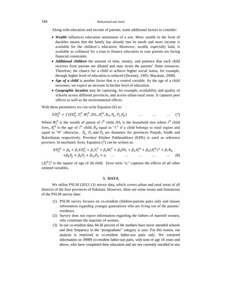
When we talk about educational mobility, we first determine whether a son falls in

the educational category of his father or otherwise. If he does then the educational status

of a son depicts persistence or immobility. However, if he does not, then there is

educational mobility either upwards or downwards. For this purpose we compute

contingency tables—Table 2.

Values of Pearson Chi square in all three cases indicate the existence of

significance correlation between levels of education for fathers’ and sons’. Results of the

data for Pakistan show that (a) frequencies of sons in the levels of education where

fathers fall are highest, or , (b) highest in the higher levels of educations than the fathers’

levels of education and, (c) lower for intermediate where the majority of sons fall in

matric. A similar pattern can be observed in the data for urban areas. However, in the

data for rural areas, we can observe that frequencies of sons whose fathers fall in the

intermediate and graduate levels of education are highest in matric. These results indicate

persistence in the level of education, with upward mobility at low levels, and downward

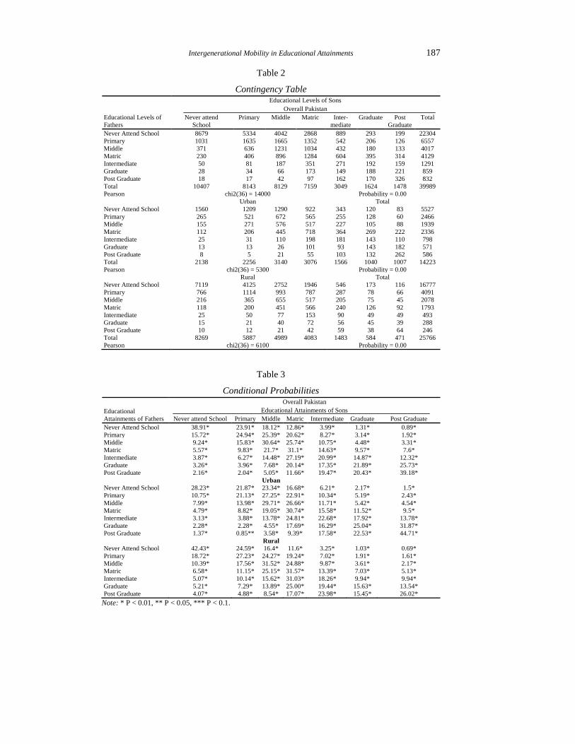
mobility at college and university levels. From the above contingency table, we compute

conditional probabilities of sons in Table 3 below. Each row of the table shows the

chances of sons to attain different levels of education given the level of education of their

fathers.

790.9 percent of the fathers and 77.3 percent of the sons fall in below matric level of education in rural

region as compared to 73.1 percent of the fathers and 56.8 percent of the sons in the same categories in urban

region.


Table 2

Contingency Table

Educational Levels of

Fathers

Educational Levels of Sons

Overall Pakistan

Never attend

School

Primary Middle Matric Inter-

mediate

Graduate Post

Graduate

Total

Never Attend School 8679 5334 4042 2868 889 293 199 22304

Primary 1031 1635 1665 1352 542 206 126 6557

Middle 371 636 1231 1034 432 180 133 4017

Matric 230 406 896 1284 604 395 314 4129

Intermediate 50 81 187 351 271 192 159 1291

Graduate 28 34 66 173 149 188 221 859

Post Graduate 18 17 42 97 162 170 326 832

Total 10407 8143 8129 7159 3049 1624 1478 39989

Pearson chi2(36) = 14000 Probability = 0.00

Urban Total


Primary 265 521 672 565 255 128 60 2466

Middle 155 271 576 517 227 105 88 1939

Matric 112 206 445 718 364 269 222 2336

Intermediate 25 31 110 198 181 143 110 798

Graduate 13 13 26 101 93 143 182 571

Post Graduate 8 5 21 55 103 132 262 586

Total 2138 2256 3140 3076 1566 1040 1007 14223


Rural Total


Primary 766 1114 993 787 287 78 66 4091

Middle 216 365 655 517 205 75 45 2078

Matric 118 200 451 566 240 126 92 1793

Intermediate 25 50 77 153 90 49 49 493

Graduate 15 21 40 72 56 45 39 288

Post Graduate 10 12 21 42 59 38 64 246

Total 8269 5887 4989 4083 1483 584 471 25766


Table 3

Conditional Probabilities

Educational

Attainments of Fathers

Overall Pakistan

Educational Attainments of Sons

Never attend School Primary Middle Matric Intermediate Graduate Post Graduate

Never Attend School 38.91* 23.91* 18.12* 12.86* 3.99* 1.31* 0.89*

Primary 15.72* 24.94* 25.39* 20.62* 8.27* 3.14* 1.92*

Middle 9.24* 15.83* 30.64* 25.74* 10.75* 4.48* 3.31*

Matric 5.57* 9.83* 21.7* 31.1* 14.63* 9.57* 7.6*

Intermediate 3.87* 6.27* 14.48* 27.19* 20.99* 14.87* 12.32*

Graduate 3.26* 3.96* 7.68* 20.14* 17.35* 21.89* 25.73*

Post Graduate 2.16* 2.04* 5.05* 11.66* 19.47* 20.43* 39.18*

Urban


Primary 10.75* 21.13* 27.25* 22.91* 10.34* 5.19* 2.43*

Middle 7.99* 13.98* 29.71* 26.66* 11.71* 5.42* 4.54*

Matric 4.79* 8.82* 19.05* 30.74* 15.58* 11.52* 9.5*

Intermediate 3.13* 3.88* 13.78* 24.81* 22.68* 17.92* 13.78*

Graduate 2.28* 2.28* 4.55* 17.69* 16.29* 25.04* 31.87*

Post Graduate 1.37* 0.85** 3.58* 9.39* 17.58* 22.53* 44.71*

Rural


Primary 18.72* 27.23* 24.27* 19.24* 7.02* 1.91* 1.61*

Middle 10.39* 17.56* 31.52* 24.88* 9.87* 3.61* 2.17*

Matric 6.58* 11.15* 25.15* 31.57* 13.39* 7.03* 5.13*

Intermediate 5.07* 10.14* 15.62* 31.03* 18.26* 9.94* 9.94*

Graduate 5.21* 7.29* 13.89* 25.00* 19.44* 15.63* 13.54*

Post Graduate 4.07* 4.88* 8.54* 17.07* 23.98* 15.45* 26.02*

Note: * P < 0.01, ** P < 0.05, *** P < 0.1.


High persistence can be observed in educational attainment, as values in the

principal diagonal are higher than the values of off diagonal in most cases. This

persistence is highest for the extreme categories. A son of a father who is in “never attend

school” has a 38.91 percent chance of falling in the same “never attend school” category.

His chance to move to the highest level of education (postgraduate) is only 0.89 percent.

Similarly, high rigidity can be observed in the “postgraduate” level where the probability

of a son to attain “postgraduate” level of education is 39.81 percent given that his father

has also attained “postgraduate” level of education, and his probability to fall in “never

attend school” is only 2.16 percent.

A panoramic view of the results suggests that although there is persistence in

educational attainment, on average the chances of a son to achieve the same level of

education as his father did, or more, are higher than his chances to lag behind his father’s

educational level.8 Similarly, from the figures in the columns we can observe that when a

father is switching to higher levels of education, the probability of the son to remain in

lower levels of education decreases while his probability to attain high levels of

education increases. Our findings comply with the earlier findings by Javed and Irfan

(2014). Results of Labour (2011) for China also depict a similar pattern, but relatively

more mobility is observed for the lowest category (primary level of education), in this

study.

Rural and urban area data present a slightly different pattern. While rigidity is

greater at a higher level of education in urban areas, a higher persistence can be observed

in the lower levels of education in rural areas.9 Urban data reflect an upward mobility in

the “Graduate” category, while rural data exhibit downward mobility for the same level

of education. Here, our results contradict Javed and Irfan (2014) who find a larger

persistence in rural areas, and more downward mobility in urban areas at the “Graduate”

level.

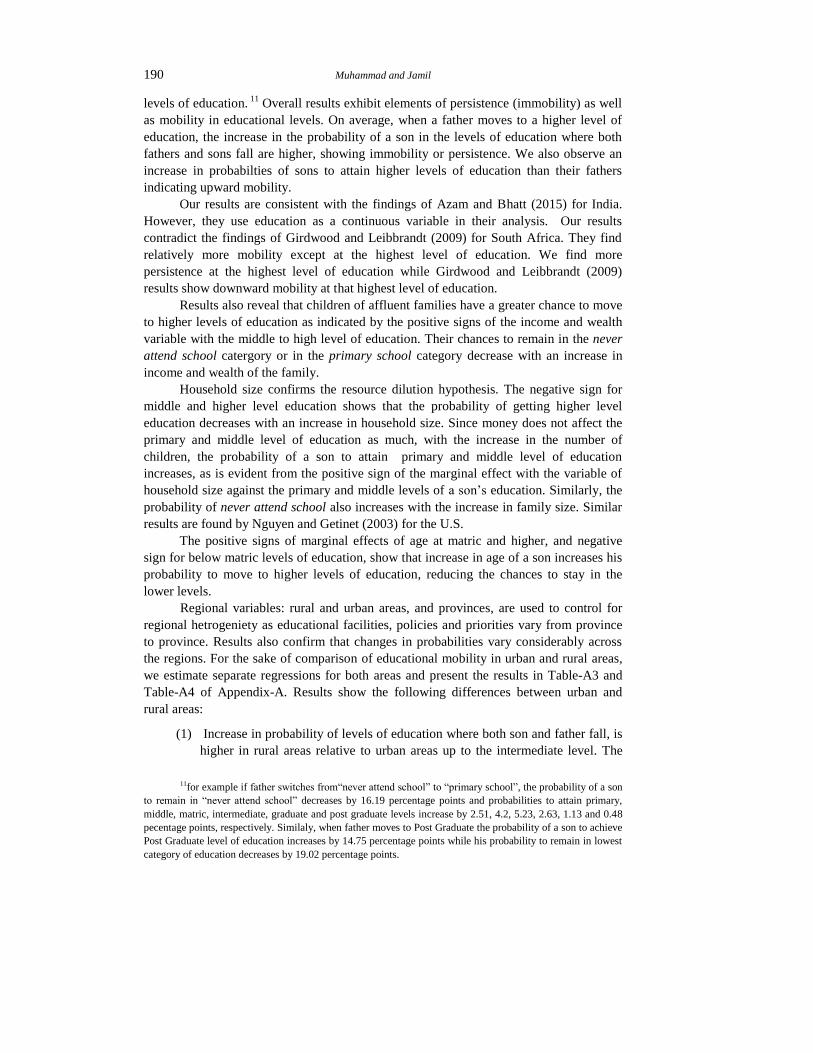
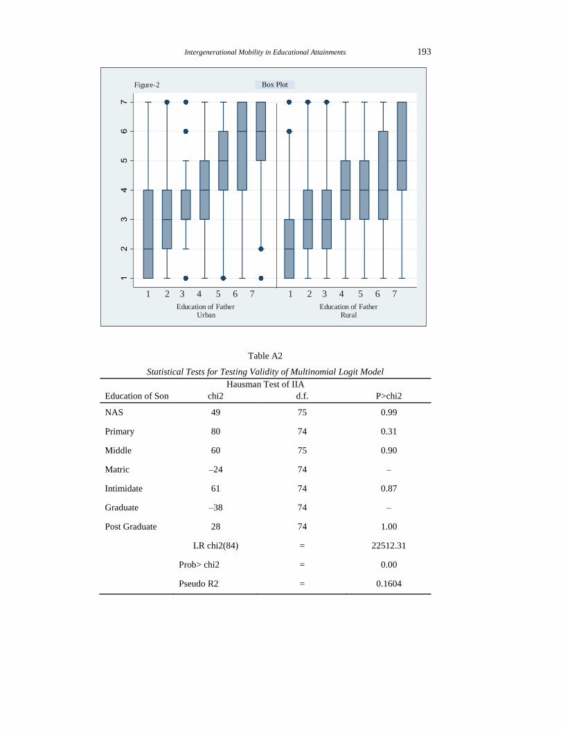
Quartile distributions of sons’ education over fathers’ education are presented in

Figure 1 and Figure 2 (Appendix-A) for overall data, and for urban-rural areas

respectively. Figures reflect persistence in education as levels of education of sons

increase, with the increase in levels of education of their fathers. Figure 1 also reflects

upward mobility at low levels and downward mobility at high levels of education in the

overall data for Pakistan. However, a comparison of the urban and rural population

exhibits more downward mobility at college and university levels of education (Figure 2).

We conclude from the above results that chances of a son attaining high (low)

level of education increase when the father also has a high (low) level of education. This

shows a sort of persistence in educational attainments; sons imitate fathers. Results also

reveal that on average, sons get a higher level of education as compared to their fathers

and thus on average the status of sons increases in terms of educational attainment as

compared to their fathers.

8 We have also computed overall downward mobility, immobility and upward mobility for overall

Pakistan as well as for urban and rural regions given in Table-A1 in Appendix-A 9In urban region, the probability of a son to remain in “never attend school” category is 28.23 percent if

his father is also in “never attend school” while the same probability is 42.43 percent in rural regions. On the

other hand, probabilities of sons to attain the “post graduate” level of education given that father also attains

“post graduate” are 44.71 percent and 26.02 percent in urban and rural regions, respectively.


Therefore, we have related the educational level of a son to the educational level of

his father to find mobility without bringing the role of other variables into the picture. To

find the impact of other variables with the educational level of a father10

we estimate

Equation (8) using multinomial logit model (MNLM). Results are in Table 4 below.

Table 4

Marginal Effects (overall Pakistan)

NAS_S PMY_S MDL_S MTC_S INT_S GRD_S PGR_S

PMY_F -0.1619* 0.025* 0.042* 0.0523* 0.0264* 0.0113* 0.0048*

(0.0054) (0.006) (0.006) (0.0056) (0.0037) (0.0025) (0.0022)

MDL_F -0.1767* -0.033* 0.065* 0.0779* 0.0401* 0.0160* 0.0104*

(0.0072) (0.0074) (0.0075) (0.0071) (0.0047) (0.0030) (0.0026)

MTC_F -0.2061* -0.072* 0.0143** 0.1296* 0.0644* 0.0432* 0.0268*

(0.0074) (0.0074) (0.0075) (0.0078) (0.0052) (0.0036) (0.0028)

INT_F -0.2241* -0.1012* -0.0183 0.1163* 0.1186* 0.0683* 0.0404*

(0.0127) (0.0125) (0.0126) (0.0134 (0.0103) (0.0067) (0.0048)

GRD_F -0.1873* -0.109* -0.0701* 0.0845* 0.0948* 0.1024* 0.0851*

(0.0208) (0.0178) (0.0155) (0.0172) (0.0123) (0.0096) (0.0075)

PGR_F -0.1902* -0.139* -0.0843* 0.0200 0.1410* 0.1047* 0.1475*

(0.0248) (0.0191) (0.0173) (0.0173) (0.0158) (0.0106) (0.0103)

Income -0.0042* -0.002 0.0022* 0.0025* 0.0009* 0.0002*** 0.0002*

(0.0012) (0.0011) (0.0008) (0.0006) (0.0003) (0.0001) (0.0001)

Wealth -0.010* -0.0027* 0.0023* 0.0043* 0.0022* 0.0016* 0.0022*

(0.0002) (0.0002) (0.0002) (0.0002) (0.0001) (0.0001) (0.0001)

H. Size 0.0026* 0.0032* 0.00005*** -0.0030* -0.0012* -0.0006** -0.0011*

(0.0006) (0.0006) (0.0006) (0.0005) (0.0004) (0.0003) (0.0002)

Age -0.0193* -0.0172* -0.0065* 0.0102* 0.0088* 0.0113* 0.0128*

(0.0016) (0.0017) (0.0018) (0.0017) (0.0012) (0.0010) (0.0010)

Age Sq. 0.0003* 0.0002* 0.0001*** -0.0001* -0.0001* -0.0002* -0.0002*

(0.00003) (0.00003) (0.00003) (0.00003) (0.00002) (0.00002) (0.00002)

Rural -0.0369* -0.0019 0.0044 0.0202* 0.0087* 0.0001 0.0054*

(0.0053) (0.0051) (0.0046) (0.0043) (0.0030) (0.0022) (0.0021)

Punjab 0.0276* 0.0664* 0.0405* -0.0574* -0.0328* -0.0134* -0.0308*

(0.0058) (0.0057) (0.0061) (0.0056) (0.0038) (0.0027) (0.0028)

Sindh 0.0609* 0.0287* -0.0805* -0.0336* 0.0280* 0.0133* -0.0168*

(0.0063) (0.0060) (0.0062) (0.0064) (0.0048) (0.0034) (0.0033)

Baloch 0.0190* 0.0548* -0.0652* 0.0135*** -0.0113** 0.0083** -0.0191*

(0.0063) (0.0064) (0.0066) (0.0072) (0.0050) (0.0042) (0.0040)

Constant 0.2602* 0.2036* 0.2033* 0.1790* 0.0762* 0.0406* 0.0370*

(0.0019) (0.0020) (0.0019) (0.0019) (0.0013) (0.0009) (0.0008)

Note: * P < 0.01, ** P < 0.05, *** P < 0.1. Standard errors are in parentheses. NAS=never attend school, PMY

= Primary school, MDL=Midlle, MTC = Matric, INT = Intermediate, GRD = Graduate, PGR= Post

Graduate, _F= father, _S= son.

Marginal effects, calculated from multinomial logit estimates, show that the

probability of a son to remain in low levels of education decreases, and his probability to

attain high levels of education increases, when his father switches from lower to higher

10Model was estimated first by ordered logit method but assumption of parallel regression required for

ordered logit was rejected by Brant test. Further, results of Hausman test given in Table-A2 of Appendix-A,

support the assumption of “Independence of Irrelevant Alternatives” (IIA), which is required for the validity of

MNLM. Likelihood Ratio (LR) test given at the lower panel of the Table-A2, shows that overall model fits

significantly better than a model with no explanatory variable.


levels of education. 11

Overall results exhibit elements of persistence (immobility) as well

as mobility in educational levels. On average, when a father moves to a higher level of

education, the increase in the probability of a son in the levels of education where both

fathers and sons fall are higher, showing immobility or persistence. We also observe an

increase in probabilties of sons to attain higher levels of education than their fathers

indicating upward mobility.

Our results are consistent with the findings of Azam and Bhatt (2015) for India.

However, they use education as a continuous variable in their analysis. Our results

contradict the findings of Girdwood and Leibbrandt (2009) for South Africa. They find

relatively more mobility except at the highest level of education. We find more

persistence at the highest level of education while Girdwood and Leibbrandt (2009)

results show downward mobility at that highest level of education.

Results also reveal that children of affluent families have a greater chance to move

to higher levels of education as indicated by the positive signs of the income and wealth

variable with the middle to high level of education. Their chances to remain in the never

attend school catergory or in the primary school category decrease with an increase in

income and wealth of the family.

Household size confirms the resource dilution hypothesis. The negative sign for

middle and higher level education shows that the probability of getting higher level

education decreases with an increase in household size. Since money does not affect the

primary and middle level of education as much, with the increase in the number of

children, the probability of a son to attain primary and middle level of education

increases, as is evident from the positive sign of the marginal effect with the variable of

household size against the primary and middle levels of a son’s education. Similarly, the

probability of never attend school also increases with the increase in family size. Similar

results are found by Nguyen and Getinet (2003) for the U.S.

The positive signs of marginal effects of age at matric and higher, and negative

sign for below matric levels of education, show that increase in age of a son increases his

probability to move to higher levels of education, reducing the chances to stay in the

lower levels.

Regional variables: rural and urban areas, and provinces, are used to control for

regional hetrogeniety as educational facilities, policies and priorities vary from province

to province. Results also confirm that changes in probabilities vary considerably across

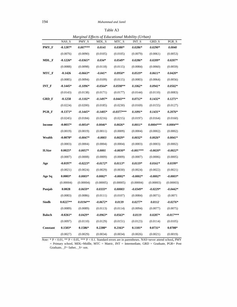
the regions. For the sake of comparison of educational mobility in urban and rural areas,

we estimate separate regressions for both areas and present the results in Table-A3 and

Table-A4 of Appendix-A. Results show the following differences between urban and

rural areas:

(1) Increase in probability of levels of education where both son and father fall, is

higher in rural areas relative to urban areas up to the intermediate level. The

11for example if father switches from“never attend school” to “primary school”, the probability of a son

to remain in “never attend school” decreases by 16.19 percentage points and probabilities to attain primary,

middle, matric, intermediate, graduate and post graduate levels increase by 2.51, 4.2, 5.23, 2.63, 1.13 and 0.48

pecentage points, respectively. Similaly, when father moves to Post Graduate the probability of a son to achieve

Post Graduate level of education increases by 14.75 percentage points while his probability to remain in lowest

category of education decreases by 19.02 percentage points.


same probability is higher in urban areas relative to rural areas for graduate

and postgraduate levels of education.

(2) In urban areas, when a father is moving from “never attend school” to any higher

level of education, the increase in probability for his son is either the maximum in

levels of education where both son and father fall, or an increase in the probability

that the son will fall in the higher level of education category than his father. In

rural areas, the probability is at maximum that the son will fall in lower levels of

education than the father will, when the father is moving from “never attend

school” to intermediate, graduate or postgraduate levels of education.

(3) When the father is advancing from “never attend school” to college or

university levels of education, the increase in probability that the son will also

attain college or higher levels of education is higher in urban than in rural

areas. These results indicate that although there is strong persistence in

educational level, upward mobility is also observed. This mobility is stronger

in urban areas as compared to rural areas. In rural areas, downward mobility

can be observed at college and university levels of education.

Affluent families in urban areas are more likely to get a higher level of education

as compared to the families in rural areas, as indicated by the larger increases in

probabilities of college and university education, due to an increase in income and wealth

in urban areas. In both urban and rural areas, the chance of a son going forward to higher

education decreases with an increase in family size. Magnitudes of the marginal effects of

age variables indicate that sons in urban areas are more likely to complete various levels

of education earlier than sons in rural areas. Finally, province dummies show significant

differences in educational mobility across the provinces.

7. CONCLUSION AND POLICY IMPLICATIONS

Intergenerational mobility in socioeconomic status represents the equality of

opportunities available to individuals in a country. It affects productivity of individuals

and thereby overall inequality and economic growth of a country. As the level of

education determines the income and other socioeconomic outcomes, we used it as a

proxy to calculate the overall socioeconomic status of an individual. We examined

intergenerational educational mobility in Pakistan, comparing the differences in urban

and rural areas as well.

We used data of PSLM survey of 2012-13. Our results reveal that percentages of

both father and son generations are high in primary education in Pakistan overall, as well

as in urban and rural data. However, percentages of sons having higher education are

higher than the percentages of fathers. Further, results of contingency tables and MNLM

revealed strong rigidity. Fathers are more likely to transmit the same level of education to

their sons. Sons of less educated fathers are more likely to remain less educated and the

sons of highly educated fathers are more likely to get higher levels of education. While

persistence in education is strong at the lower levels in urban areas, there is more

persistence at higher education levels in urban areas.

Our research showed upward mobility due to educational attainment, with urban

areas showing higher upward mobility than rural areas. We also found that higher

education positively affected increase in income and wealth of households. However, a


larger family was found to hinder mobility. Further, the chance to get college and

university education was higher for sons in urban areas, with them more likely to reach

educational levels earlier than sons in the rural areas were.

Although overall results suggest an upward mobility trend, Pakistan still lags

behind the developed world with an average schooling of 4.7 years only. There is an

urgent need for further increase in educational mobility. Government programmes to

provide funding for higher education to underprivileged students will go a long way

towards improving mobility and raising the educational levels of Pakistan’s work force.

Some policies that would help achieve the above stated objective:

Government should require mandatory enrolment of children in primary school

at a specific age. This will ensure that schooling starts at an early age.

Financial constraints of families tend to have less of an effect on the education

of children once they are enrolled in school (Bauer and Riphahn, 2009). Early

enrolment should specially be ensured in rural areas where students tend to

complete their schooling later than their counterparts in urban areas.

A carefully thought out policy of family planning to limit family size is required.

Limiting family size would affect middle-income groups only. Since low-

income families have a lack of resources to begin with, having more children

will not have the negative effect of resource dilution on this section of the

population (Steelman et al., 2002; Van Bavel, 2011).

Finally, opportunities for children stem from family support and ideology, so

reliance upon the education system solely to increase mobility may be an overly

optimistic strategy. Institutional reforms and behavioural changes are required to improve

educational mobility and thereby the socioeconomic status of the current generation.

APPENDIX

Table A1

Educational Mobility: Summary of Transition Matrices

Region Downward Mobility Immobility Upward Mobility

Pakistan Overall 12 36 52

Urban Overall 16 29 55

Rural Overall 10 39 51

Education of Father

Edu

cati

on o

f S

on

Figure-1 Box-PilotBox Plot


Table A2

Statistical Tests for Testing Validity of Multinomial Logit Model

Hausman Test of IIA

Education of Son chi2 d.f. P>chi2

NAS 49 75 0.99

Primary 80 74 0.31

Middle 60 75 0.90

Matric –24 74 –

Intimidate 61 74 0.87

Graduate –38 74 –

Post Graduate 28 74 1.00

LR chi2(84) = 22512.31

Prob> chi2 = 0.00

Pseudo R2 = 0.1604

Figure-2 Box Pilot

1 2 3 4 5 6 7 1 2 3 4 5 6 7

Education of FatherUrban

Education of FatherRural

Box Plot


Table A3

Marginal Effects of Educational Mobility (Urban)


PMY_F -0.1207* 0.007*** 0.0141 0.0380* 0.0286* 0.0290* 0.0040

(0.0076) (0.0090) (0.0105) (0.0105) (0.0079) (0.0061) (0.0053)

MDL_F -0.1226* -0.0365* 0.034* 0.0549* 0.0286* 0.0209* 0.0207*

(0.0088) (0.0098) (0.0118) (0.0115) (0.0084) (0.0060) (0.0059)

MTC_F -0.1426 -0.0663* -0.041* 0.0950* 0.0519* 0.0611* 0.0420*

(0.0085) (0.0094) (0.0109) (0.0115) (0.0083) (0.0064) (0.0056)

INT_F -0.1445* -0.1096* -0.0564* 0.0598** 0.1062* 0.0941* 0.0502*

(0.0143) (0.0138) (0.0171) (0.0177) (0.0144) (0.0110) (0.0083)

GRD_F -0.1258 -0.1102* -0.1497* 0.0443** 0.0712* 0.1432* 0.1271*

(0.0224) (0.0200) (0.0185) (0.0230) (0.0169) (0.0155) (0.0127)

PGR_F -0.1371* -0.1445* -0.1405* -0.0377*** 0.1091* 0.1431* 0.2076*

(0.0245) (0.0184) (0.0216) (0.0215) (0.0197) (0.0164) (0.0160)

Income -0.0037* -0.0054* 0.0046* 0.0026* 0.0011* 0.0004*** 0.0004**

(0.0019) (0.0019) (0.0011) (0.0009) (0.0004) (0.0002) (0.0002)

Wealth -0.0078* -0.0047* -0.0003 0.0029* 0.0032* 0.0026* 0.0041*

(0.0003) (0.0004) (0.0004) (0.0004) (0.0003) (0.0003) (0.0002)

H.Size 0.0025* 0.0057* 0.0001 -0.0030* -0.001*** -0.0020* -0.0022*

(0.0007) (0.0008) (0.0009) (0.0009) (0.0007) (0.0006) (0.0005)

Age -0.0197* -0.0223* -0.0172* 0.0113* 0.0119* 0.0161* 0.0199*

(0.0021) (0.0024) (0.0029) (0.0030) (0.0024) (0.0022) (0.0021)

Age Sq 0.0003* 0.0003* 0.0002* -0.0002* -0.0002* -0.0002* -0.0003*

(0.00004) (0.00004) (0.00005) (0.00005) (0.00004) (0.00003) (0.00003)

Punjab 0.0028 0.0659* 0.0333* 0.00003 -0.0349* -0.0229* -0.0442*

(0.0083) (0.0086) (0.0111) (0.0107) (0.0084) (0.0071) (0.0071

Sindh 0.0227** 0.0194** -0.0672* 0.0139 0.0277* 0.0112 -0.0276*

(0.0089) (0.0089) (0.0113) (0.0114) (0.0094) (0.0077) (0.0075)

Baloch -0.0261* 0.0429* -0.0963* 0.0563* 0.0119 0.0287* -0.017***

(0.0097) (0.0110) (0.0129) (0.0151) (0.0123) (0.0114) (0.0105)

Constant 0.1503* 0.1586* 0.2208* 0.2163* 0.1101* 0.0731* 0.0708*

(0.0027) (0.0029) (0.0034) (0.0034) (0.0026) (0.0021) (0.0019)



Graduate, _F= father, _S= son.


Table A4

Marginal Effects of Educational Mobility (Rural)


PMY_F -0.1829* 0.0362* 0.0578* 0.0578* 0.023* 0.0031 0.005**

(0.0072) (0.0079) (0.0073) (0.0067) (0.0040) (0.0021) (0.0020)

MDL_F -0.2119* -0.0290* 0.0788* 0.0896* 0.051* 0.0155* 0.006**

(0.0103) (0.0104) (0.0097) (0.0093) (0.0063) (0.0035) (0.0025)

MTC_F -0.2513* -0.0796* 0.0559* 0.1471* 0.073* 0.0356* 0.0192*

(0.0110) (0.0108) (0.0107) (0.0111) (0.0074) (0.0047) (0.0033)

INT_F -0.2832* -0.0844* 0.0006 0.1509* 0.1162* 0.0559* 0.044*

(0.0181) (0.0198) (0.0188) (0.0205) (0.0156) (0.0099) (0.0078)

GRD_F -0.2345* -0.1005* 0.0126 0.0965* 0.1004* 0.0759* 0.049*

(0.0312) (0.0276) (0.0272) (0.0252) (0.0184) (0.0133) (0.0097)

PGR_F -0.2272* -0.1184* -0.0350 0.049*** 0.1509* 0.0762* 0.104*

(0.0389) (0.0320) (0.0292) (0.0270) (0.0249) (0.0152) (0.0150)

Income -0.0046* -0.0001 -0.0004 0.0038* 0.0011* 0.00001** 0.0003**

(0.0016) (0.0014) (0.0011) (0.0008) (0.0004) (0.0003) (0.0001)

Wealth -0.0112* -0.0016* 0.0034* 0.0049* 0.0021* 0.0012* 0.0012*

(0.0003) (0.0003) (0.0002) (0.0002) (0.0001) (0.0001) (0.0001)

H.Size 0.0031* 0.0015 0.0004*** -0.0031* -0.0014* -0.0001* -0.0004*

(0.0008) (0.0008) (0.0007) (0.0006) (0.0004) (0.0002) (0.0002)

Age -0.0194 -0.0144* -0.0008 0.0095* 0.0075* 0.0084* 0.0093*

(0.0023* (0.0023) (0.0022) (0.0020) (0.0014) (0.0010) (0.0010)

Age Sq 0.0003 0.0002* 0.00002 -0.0001* -0.0001* -0.0001* -0.0001*

(0.00004 (0.00004) (0.00004) (0.00004) (0.00002) (0.00002) (0.00002)

Punjab 0.0397* 0.0633* 0.0454* -0.0828* -0.0339* -0.0096* -0.0221*

(0.0079) (0.0075) (0.0073) (0.0064) (0.0039) (0.0022) (0.0023)

Sindh 0.0795* 0.0334* -0.0963* -0.0574* 0.0299* 0.0177* -0.0068**

(0.0086) (0.0082) (0.0074) (0.0078) (0.0059) (0.0039v (0.0034)

Baloch 0.0366* 0.0603* -0.0541* -0.0079 -0.0198* 0.0011 -0.0162*

(0.0083) (0.0081) (0.0077) (0.0080) (0.0049) (0.0033) (0.0030)

Constant 0.3209* 0.2285* 0.1936* 0.1585* 0.0576* 0.0227* 0.0183*

(0.0026) (0.0026) (0.0024) (0.0022) (0.0014) (0.0009) (0.0008)



Graduate, _F= father, _S= son

REFERENCES

Assad, R., & Saleh, M. (2016). Does improved local supply of schooling enhance

intergenerational mobility in education? evidence from Jordan. The World Bank

Economic Review, lhw041.

Azam, M., & Bhatt, V. (2015) Like father, like son? Intergenerational educational

mobility in India. Demography, 52(6), 1929–1959.

Bauer, P., & Riphahn, T. R. (2009). Kindergarten enrolment and the intergenerational

transmission of education. Institute for the Study of Labour (IZA), Bonn. (Discussion

Paper No. 4466).

Becker, G. S., & Tomes, N. (1976). Child endowments and the quantity and quality of

children. Journal of Political Economy 84(4), S143–S162.

Becker, G. S., & Tomes, N. (1979). An equilibrium theory of the distribution of income

and intergenerational mobility. Journal of Political Economy, 87(6), 1153–1189.

Becker, G. S., & Tomes, N. (1986). Human capital and the rise and fall of families.

Journal of Labour Economics, 4(3), S1–S39.


Becker, G., Kominers, S., Murphy, K. M., & Spenkuch, J. R. (2015). A theory of

intergenerational mobility. Available at SSRN: hhttp://dx.doi.org/10.2139/

ssrn.2652891.

Black, S. E., & Devereux, P. J. (2011). Recent developments in intergenerational

mobility. Handbook of Labour Economics, 4(B), Ch-16, 1487–1541.

Blanden, J. (2009). How much can we learn from international comparisons of

intergenerational mobility? London School of Economics and Political Science, LSE

Library.

Burns, J. (2001). Inheriting the future: The role of family background and neighborhood

characteristics in child schooling outcomes in South Africa. Department of

Economics, University of Cape Town, Cape Town.

Cheema, A., & Naseer, M. F. (2013). Historical inequality and intergenerational

educational mobility: The dynamics of change in rural Punjab. The Lahore Journal of

Economics, 18(special edition), 211.

Downey, D. B. (1995). When bigger is not better: Family size, parental resources, and

children’s educational performance. American Sociological Review, 60(5), 746–761.

Galton, F. (1886). Regression towards mediocrity in hereditary stature. The Journal of the

Anthropological Institute of Great Britain and Ireland, 15, 246–263.

Girdwood, S., & Leibbrandt, M. (2009). Intergenerational mobility: Analysis of the NIDS

wave 1 dataset. National Income Dynamics Study Discussion Paper, 15.

Guryan, J., Hurst, E., & Kearney, M. (2008). Parental education and parental time with

children. The Journal of Economic Perspectives, 22(3), 23–46

Havinga, I. C., Mohammad, F., Cohen, S. I., & Niazi, M. K. (1986). Intergenerational

mobility and long-term socio-economic change in Pakistan [with Comments]. The

Pakistan Development Review, 25(4), 609–628.

Hertz, T., Jayasundera, T., Piraino, P., Selcuk, S., Smith, N., & Verashchagina, A.

(2007). The inheritance of educational inequality: International comparisons and fifty-

year trends. The BE Journal of Economic Analysis & Policy, 7(2), 1–46.

Javed, S. A., & Irfan, M. (2014). Intergenerational mobility: Evidence from Pakistan

panel household survey. The Pakistan Development Review, 53(2), 175–203

Labar, K. (2011). Intergenerational mobility in China. (Discussion paper). [online]

http://halshs.archives-ouvertes.fr/halshs-00556982/

Lillard, L. A., & Willis, R. J. (1994). Intergenerational educational mobility: Effects of

family and state in Malaysia. Journal of Human Resources, 29(4), 1126–1166.

Loury, G. C. (1981). Intergenerational transfers and the distribution of earnings.

Econometrica: Journal of the Econometric Society, 49(4), 843–867.

Majumder, R. (2010). Intergenerational mobility in educational and occupational

attainment: A comparative study of social classes in India. Margin: The Journal of

Applied Economic Research, 4(4), 463–494.

Maralani, V. (2008). The changing relationship between family size and educational

attainment over the course of socioeconomic development: Evidence from Indonesia.

Demography, 45(3), 693–717.

Mare, R. D. (1980). Social background and school continuation decisions. Journal of the

American statistical Association, 75, 295–305.

http://dx.doi.org/10.2139/ssrn.2652891

http://dx.doi.org/10.2139/ssrn.2652891


Meltzer, D. O. (1992). Mortality decline, the demographic transition, and economic

growth. Department of Economics, University of Chicago.

Nguyen, A., & Getinet, H. (2003). Intergenerational mobility in educational and

occupational status: Evidence from the US (No. 1383). University Library of Munich,

Germany.

Sewell, W., and R. Hauser, R. (1975). Education, Occupation, and Earnings:

Achievements in the Early Career. New York: Academic Press.

Solon, G., Barsky, R., & Parker, J. A. (1994). Measuring the cyclicality of real wages:

How important is composition bias? The Quarterly Journal of Economics, 109(1), 1–

25.

Soltow, L. (1965). Towards income equality in Norway. Madison, University of

Wisconsin Press.

Spielauer, M. (2004). Intergenerational educational transmission within families: An

analysis and micro simulation projection for Austria. Vienna Yearbook of Population

Research, 253–282.

Steelman, L.C., Powell, B., Werum, R., and Carter, S. (2002). Reconsidering the effects

of sibling configuration: Recent advances and challenges. Annual Review of

Sociology, 28, 243–269.

UNDP (2015). Human Development Report. New York, USA.

Van Doorn, M., Pop, I., & Wolbers, M. H. J. (2011). Intergenerational transmission of

education across European countries and cohorts. European Societies, 13(1), 93–117.

Wolff, P., & Van Slijpe, A. R. D. (1973). The relation between income, intelligence,

education and social background. European Economic Review, 4(3), 235–264.

Documents

Intergenerational Mobility in Educational Attainments