Embed Size (px)
DESCRIPTION
papers
Citation preview

Nc
LC
a
ARRA
KE
1
ahtCnrt
ayrvDdstw
jg
h0
Energy and Buildings 76 (2014) 238–248
Contents lists available at ScienceDirect
Energy and Buildings
j ourna l ho me pa g e: www.elsev ier .com/ locate /enbui ld
umerical study of earth-to-air heat exchanger for three differentlimates
. Ramírez-Dávila, J. Xamán ∗, J. Arce, G. Álvarez, I. Hernández-Pérezentro Nacional de Investigación y Desarrollo Tecnológico, CENIDET-DGEST-SEP, Prol. Av. Palmira S/N, Col. Palmira, Cuernavaca, Morelos CP 62490, Mexico
r t i c l e i n f o
rticle history:eceived 2 November 2013eceived in revised form 14 February 2014ccepted 22 February 2014
eyword:arth-to-air heat exchanger
a b s t r a c t
A numerical study was conducted for prediction the thermal behavior of an Earth-to-Air Heat Exchanger(EAHE) for three cities in México. The climate conditions correspond to an extreme heat in summer andlow temperature in winter (Cd. Juárez, Chihuahua), mild weather (México city) and hot weather (Mérida,Yucatán). A Computational Fluid Dynamics code based on the Finite Volume Method has been developedin order to model the EAHE. Simulations have been conducted for sand, silt and clay soil textures for thecities of Cd. Juárez, México city and Mérida, respectively. Also, for different Reynolds numbers, Re = 100,500, 1000, 1500 through one year. For Cd. Juárez, and México city, simulation results reveal that the
thermal performance of the EAHE is better in summer than in winter, decreasing the air temperature inan average of 6.6 and 3.2 ◦C for summer and increasing it in 2.1 and 2.7 ◦C for winter, respectively. Bycontrast for Mérida, EAHE had its best thermal performance in winter, increasing the air temperature in3.8 ◦C. It is concluded that the use of EAHEs is appropriate for heating or cooling of buildings in lands ofextreme and moderate temperatures where the thermal inertia effect in soil is higher.© 2014 Elsevier B.V. All rights reserved.
. Introduction
Nowdays, most of the energy demand in buildings is used forir-conditioning, which runs by burning fossil fuels, however, itsigh cost and negative environmental impact makes it necessaryo implement passive systems to reduce the energy consumption.oupling an earth-to-air heat exchanger to a building is an alter-ative to improve thermal comfort at low cost, reducing or eveneplacing the use of active systems by taking advantage of soil’shermal inertia.
Recent studies aimed to evaluate the temperature profiles in soilre still implementing 1-D analytic formulation proposed over 50ears ago by Carslaw and Jaeger [1], that are still distant from rep-esenting reality since they do not consider soil’s thermophysicalariation [2–9]. A study of this kind was carried out by Salah El-in [10], who predicted the variation of the soil temperature withepth in a 1-D model based on an energy balance at the ground
urface. They considered the variation of the solar radiation, airemperature and latent heat flux due to evaporation; however, itas considered that soil has uniform thermophysical properties.∗ Corresponding author. Tel.: +52 777 3 62 77 70; fax: +52 777 3 62 77 95.E-mail addresses: atthedrive [email protected] (L. Ramírez-Dávila),
[email protected] (J. Xamán), [email protected] (J. Arce),[email protected] (G. Álvarez), [email protected] (I. Hernández-Pérez).
ttp://dx.doi.org/10.1016/j.enbuild.2014.02.073378-7788/© 2014 Elsevier B.V. All rights reserved.
In regard with the studies focused in EAHEs, those that arebased in thermodynamics energy balance do not represent thephenomena in an appropriate way since the air flow through thepipe is not considered by disregarding its velocity [7,11–13]. One ofthese studies was conducted by Cucumo et al. [12], who considereda one-dimensional transient study where thermal perturbation insoil and water condensation inside of the heat exchanger tubeswere taken in to account. However, the variation of soil’s ther-mophysical properties has been disregarded. Costa [14] is theexception in these kinds of studies, who conducted a thermody-namical study where the air mass flow rate through the pipe isactually considered, but the study of the soil temperature pro-file is one-dimensional. Also, it is considered that the convectivecoefficient is a known value, but in reality it is not.
On the other hand, by using computational fluid dynamics,most of the numerical studies consider the existence of an air flowthrough the pipe in laminar or turbulent flow regime [2,4,15–22].However, these assume that the convective coefficient is a knownparameter, when in a real phenomenon; it is not. From the authors’knowledge, the only work that doesn’t consider the convectivecoefficient as a known value was published by Sehli et al. [23]. How-ever, the thermal influence that other dimensions could have in
their results is disregarded, because the study was in 1-D. Anotherinteresting numerical approach was carried out by Yoon et al. [22]who modeled the circular pipes as rectangular ducts applying thesame peripheral length as the circular pipe in order to simplify the
L. Ramírez-Dávila et al. / Energy and Buildings 76 (2014) 238–248 239
Nomenclature
Cp specific heat, J kg−1 K−1
G solar radiation, W/m2
Hy depth of the soil, mP pressure, PaQ heat flux, W/m2
Ra Rayleigh numberRe Reynolds numberT temperature, ◦CTout
ave air average temperature at the outlet, ◦Cu, v horizontal and vertical velocities, m/sx, y dimensional coordinates, m
Greek symbols˛ thermal diffusivity, m2 s−1
ε emissivity� thermal conductivity, W m−1 K−1
� dynamic viscosity, kg m−1 s−1
� density, kg m−3
Subscriptsave averagecond conduction heat transferconv convection heat transfer
shms3aIhbasu
rttcrdacwatpdTtdeoi
elat
Table 1Geometric dimensions for the EAHE.
Section Dimension
Soil’s depth Hy = 12 mPipe depth Hy3 = 10 mPipe diameter Hx2 = Hx4 = Hy2 = 0.15 m
rad radiation heat transfer
tudy without affecting accuracy in the results. This approximationas been adopted in the present work. A study to consider 3-D earthodeling was published by Florides et al. [17]. They conducted a
ensitive study of an EAHE with a ‘U’ pipe configuration using a-D mathematical model for heat conduction in earth, and a 1-Dpproach for mass air flow and convective heat transfer in the pipe.t was observed that the larger the diameter of the pipe, the moreeat flux will be transferred to the soil. Same effect is also obtainedy increasing soil’s thermal conductivity. Bojic et al. [16] proposed
model for multi-pipes. However, the heat transfer between theide pipes is not considered since a one-dimensional model wassed to predict temperature in the ground.
In regard to the experimental studies, they provide reliableesults describing EAHE thermal behavior under specific condi-ions [24,25] and its importance lies in the fact that they establishhe basis for validation of theoretical studies. However, the finan-ial investment and time required to set them up are high, whichepresents a restriction for this kind of studies. Amara et al. [26]etermined the viability of using an EAHE for air-conditioning in
building in Adrar, Algeria. The pipe was buried in a depth wherelimatic changes in the surface can’t influence soil’s temperature,hich is close to the average annual temperature. Therefore, the air
t the outlet of the pipe has the tendency to reach this temperaturehe whole year, lowering the thermal impact from the outdoor tem-erature. Ozgener et al. [27] conducted an exergoeconomic test toetermine the optimal design of an EAHE for a greenhouse in Izmir,urquia. The results show that the main sources of exergy destruc-ion are the pipe and the fan. The fan is a main source of exergyestruction due to losses related with mechanical and electricalfficiencies. They concluded that the implementation of method-logies aimed in thermo-economical optimization can contributen finding the optimal design for an EAHE.
Based on this brief literature review for the studies aimed to
valuate the ground temperature profile, it is concluded that ana-ytical one-dimensional formulations proposed more than 50 yearsgo [1] continue to be implemented. Such formulations do notake in to account elements that allow obtaining more realisticPipe length Hx3 = 5 mLength of soil at left and right sides Hx1 = Hx5 = 0.5 m
results, like the variation of soil’s thermophysical properties. Whenit comes to heat exchanger studies, those based in thermodynamicsenergy balance do not represent the phenomena in an appropri-ate way since the air velocity is considered negligible, therefore,the air flow through the pipe is not taken in to account. On theother hand, most of the numerical models do consider the pres-ence of an air flow going through the pipe in a laminar or turbulentregime. Nevertheless, it is assumed that the convective coefficientis a known value, when in reality it is not. It is worth mentioningthat Sehli et al. [23] do not consider that the convective coefficientis a known quantity. However, they used a one-dimensional heattransfer model for the pipe, disregarding the influence that a seconddimension could have on the results. Furthermore, experimentalstudies contribute with reliable results about the thermal behaviorof an EAHE under certain conditions. Its importance lies in the factthat they constitute the basis for validation of theoretical studiesbut the cost of investment and installation time required are high,which is a limiting factor in this kind of studies.
According to this, it is important to conduct new studies basedon more accurate considerations in order to get results closer toreality. Therefore, considerations in the present work allow a con-jugated heat transfer bi-dimensional study between the pipe andthe soil (EAHE), which is the goal of this article. Additionally, theconvective coefficient is not considered as a known value. The EAHEthermal behavior is evaluated under Cd. Juárez, México city andMérida’s climatic conditions for one year in order to determine itsimpact at the outlet pipe temperature.
2. Physical model
The system subject to study in the present work is shown inFig. 1 (where its boundaries are delimited by dashed lines). For thetheoretical study of soil the following considerations are made: (a)Energy transfer is bi-dimensional, (b) Temperature in soil remainsconstant after 10 m depth and reaches the outdoors annual averagetemperature and (c) Evaporation of water is only considered in thesurface of the ground. For the study of the pipe, the following con-siderations are taken into account: (d) Pipe’s circular cross sectionis modeled as a square cross section. Also, the thermal influenceof the pipe is disregarded due to its thickness; it is so small that itis negligible, (e) Condensation and evaporation inside of the pipeare not taken into account, (f) The dominant heat transfer mecha-nism is convection and (g) The air is in a laminar flow regime. Theconsideration (d) is adopted to simplify the calculations using theCartesian coordinate system without affecting the accuracy in theresults [4,22].
The geometric dimensions of the EAHE system are shown inTable 1.
3. Mathematical model
Soil is considered a solid medium where heat is transferred
by conduction. On the other hand, there is convective heat trans-fer in laminar flow regime through the pipe, and a heat exchangebetween the walls of the pipe and the soil. These phenomena are
240 L. Ramírez-Dávila et al. / Energy and Buildings 76 (2014) 238–248
del w
mt
i
3
−
w
Fig. 1. EAHE physical mo
odeled in the Cartesian coordinate system and described by con-inuity, momentum and energy equations [28]:
∂(�u)∂x
+ ∂(�v)∂y
= 0 (1)
∂(�uu)∂x
+ ∂(�vu)∂y
= −∂P
∂x+ ∂
∂x
[�
∂u
∂x
]+ ∂
∂y
[�
∂u
∂y
](2)
∂(�uv)∂x
+ ∂(�vv)∂y
= −∂P
∂y+ ∂
∂x
[�
∂v∂x
]+ ∂
∂y
[�
∂v∂y
](3)
∂(�uT)∂x
+ ∂(�vT)∂y
= ∂
∂x
[�
CP
∂T
∂x
]+ ∂
∂y
[�
CP
∂T
∂y
](4)
The boundary conditions for the above equations are as follow-ng.
.1. North boundary (y = 0)
The next energy balance [7] is used for the ground surface:
�∂T
∂y|y=0 = CE − LR + SR − LE (5)
here
a) CE is the convective energy exchanged between the air and soilsurface:
CE = hsur (Tamb) (6)
Tamb is the air temperature above the ground surface and hsur
is the convective heat transfer coefficient at the soil surface andcan be calculated from the following equation:( ( velwind
))
hsur = 5.678 0.775 + 0.350.304if velwind < 4.88 (7)
hsur = 5.678
(0.775 + 0.35
(velwind
0.304
)0.78)
if velwind≥4.88 (8)
ith boundary conditions.
b) LR is the long-wave radiation for horizontal surfaces:
LR = ε �R (9)
ε is the emissivity of the ground surface and �R is a termwhich depends on the relative humidity of the ground and theair above the ground surface, on the effective sky temperatureand on the soil radiative properties. A value of 63 W/m2 is a goodapproximation for this variable [11].
c) SR is the solar radiation absorbed from the ground surface:
SR = ˛G (10)
˛ is a coefficient depending on the ground surface absorptivityand its illumination and G is the incident solar energy (W/m2).
d) LE is the latent heat flux from the ground surface due to evapo-ration.
LE = 0.0168 fhsur [(aTamb + b) − HR (aTamb + b)] (11)
3.2. South boundary (y = Hy)
Ground temperature remains constant beyond this boundary(10 m depth), which approaches the annual average air tempera-ture [21]. Therefore, it can be considered: ∂T
∂y= 0.
3.3. East and west boundaries (x = 0 and x = Hx)
Adiabatic conditions are used for this boundary since any ther-mal influence coming from these boundaries is disregarded: ∂T
∂x= 0.
On the other hand, pipe’s boundary conditions are as follows.
3.4. Inlet air
It is at the outdoors’s temperature and constant velocity (v =f (Re), u = 0) which is in function of four different Reynoldsnumbers.

L. Ramírez-Dávila et al. / Energy and Buildings 76 (2014) 238–248 241
3
i
tlcocdg
4
tsseaiN
itbetit
a
dVs
TN
Table 3Average Nusselt number in the hot wall for aspect ratios of 2, 4, 6 and 10.
Ra Mohamad et al. [30] Present study Absolute differencespercentage (%)
A = 2103 4.34 4.10 5.53104 4.28 4.03 5.78105 5.91 5.92 0.25106 12 11.82 1.52
A = 4103 4.23 3.99 6.63104 4.18 3.95 5.51105 5.35 5.26 1.53106 10.42 10.34 0.76
A = 6103 4.21 3.96 5.96104 4.18 3.93 5.88105 5.10 5.01 1.73106 9.61 9.65 0.37
A = 10103 4.18 3.94 5.82104 4.17 3.92 5.94
5
variables is 10 .The methodology previously described can be summarized as
follows:
Fig. 2. Non-uniform grid.
.5. Outlet air
Developed flow conditions are used for temperature and veloc-ty: ∂T
∂y= 0, ∂u
∂y= 0 and ∂v
∂y= 0.
The system is treated as if it all were a fluid. Therefore,hermophysical properties assigned are variable according to theocation in the system, where its values are recalculated at theontrol-volume faces by interpolations. Subsequently, a blocking-ff method is used, which consists of setting up the velocityomponents equal to zero in the solid region, this way, the hydro-ynamic effect in soil gets restricted and heat transfer is thenoverned only by conduction.
. Methodology
In order to solve the governing equations, a CFD code based inhe finite volume method (FVM) has been implemented, which con-ists of generating a grid by sub-dividing the domain in to smallerub-domains, where � is transported [28]. In this case, it is nec-ssary to use a non-uniform grid refinement that is finer in thereas with the larger � variations. The non-uniform grid generateds shown in Fig. 2, its size changes depending on the position (Nx1,x2, Nx3, Ny1, Ny2 y Ny3).
It is intended to find the value of � for the internal nodes, whichs transported from the external nodes; where its value is given byhe system’s boundary conditions that have been set up since theeginning. In order to know the internal nodes value for �, it is nec-ssary to establish a system of algebraic equations by discretizinghe differential equations that govern the physical phenomenon byntegrating its terms over the control volume. Finally, this leads tohe discretization equation [28]:
P�P = aE�E + aW �W + aN�N + aS�S + b (12)
Since in the governing differential equation for convection-iffusion the velocities field is unknown, they need to be calculated.elocity is governed by the momentum equations, where a pres-ure term is included, which is another unknown variable to
able 2odes distribution in EAHE.
Section Number of nodes
Nx1, Nx5 21Nx2, Nx4, Ny2 71Nx3 91Ny1 41Ny3 201
10 4.81 4.69 2.56106 8.58 8.64 0.81
calculate, that increases nonlinearity of the equations. This prob-lem has been tackled by implementing the SIMPLEC algorithm, apressure-velocity coupling technique that allows calculating theflow field [29].
It is known that the solution of the algebraic equationsapproaches the exact solution once a pre-establish convergencecriterion is reached, which has to be rigorous enough to warrantythat the change of � in the subsequent iterations is negligible. Inthe present work the convergence criterion for all the unknown
−10
Fig. 3. C-shaped thermosyphon physical model.

242 L. Ramírez-Dávila et al. / Energy and Buildings 76 (2014) 238–248
0.0
0.2
0.4
0.6
0.8
1.0
-0.4 -0.2 0.0 0.2 0.4 0.6 0.8
u *
y *
Expe rimenta l Results Pre sen t Stu dy
0.0
0.2
0.4
0.6
0.8
1.0
-0.2 0.0 0.2 0.4 0.6 0.8
u *
y *
Experimen tal Resu lts Prese nt Study
(a) (b)
0.0 0.5 1.0 1.5 2.0 2.5 3.0-0.4
-0.2
0.0
0.2
0.4
0.6
0.8
1.0
1.2
Expe rime nta l Results Pre sen t Stu dy
u *
x *
0.0 0.5 1.0 1.5 2.0 2.5 3.0
-0.4
-0.3
-0.2
-0.1
0.0
0.1
0.2
0.3
0.4
u *
x *
Expe rime ntal Results Present Stud y
(c) (d)
TC
Fig. 4. Comparison of the u∗-velocity between Nielsen (1990) and the p
able 4limatic conditions in Cd. Juárez, Chihuahua for the year 2010.
Month Average temp. (◦C) Data corresponding to therepresentative day of the month
Representative day of the month Max temp. (◦
Jan 8.1 31-Jan –
Feb 10.4 22-Feb –
Mar 14.9 17-Mar –
Apr 19.4 11-Apr 25.3
May 25.0 20-May 31.1
Jun 28.2 19-Jun 33.3
Jul 28.7 9-Jul 33.6
Aug 27.3 19-Aug 31.3
Sep 24.2 4-Sep 29.1
Oct 19.2 11-Oct –
Nov 12.0 11-Nov –
Dec 7.3 18-Dec –
resent study in: x∗ = 1.0, (b) x∗ = 2.0, (c) y∗ = 0.972 y (d) y∗ = 0.028.
Average data corresponding to therepresentative day of the month
C) Min temp. (◦C) RH (%) Irradiance (W/m2) Wind speed (m/s)
-0.6 53.3 312.3 3.43.2 36.8 461.1 4.37.5 30.0 392.8 4.8– 26.5 593.3 3.4– 22.0 715.8 2.2– 18.2 565.3 5.3– 38.5 574.0 4.6– 50.3 282.0 2.9– 42.1 316.9 2.1
11.3 39.0 394.6 1.53.3 48.1 339.5 3.20.8 42.7 415.2 3.2

L. Ramírez-Dávila et al. / Energy and Buildings 76 (2014) 238–248 243
Table 5Climatic conditions in México city for the year 2010.
Month Average temp. (◦C) Data corresponding to therepresentative day of the month
Average data corresponding to therepresentative day of the month
Representative day of the month Max temp. (◦C) Min temp. (◦C) RH (%) Irradiance (W/m2) Wind speed (m/s)
Jan 13.8 13-Jan – 1.8 43.0 369.8 2.4Feb 15.5 15-Feb – 4.1 40.0 408.0 7.0Mar 17.5 3-Mar – 6.8 33.0 462.5 3.3Apr 18.8 12-Apr 27.2 – 40.0 451.7 3.1May 19.1 20-May 28.0 – 46.0 570.4 3.2Jun 18.0 6-Jun 27.9 – 58.0 380.5 3.2Jul 17.7 25-Jul 25.1 – 63.0 375.6 3.0Aug 17.6 14-Aug 25.0 – 64.0 382.7 3.0Sep 17.0 10-Sep 25.2 – 69.0 328.6 2.9Oct 16.6 7-Oct – 7.0 63.0 329.5 3.0Nov 14.6 7-Nov – 3.1 55.0 380.6 2.7Dec 13.9 2-Dec – 3.2 49.0 359.8 2.3
Table 6Climatic conditions in Mérida, Yucatán for the year 2010.
Month Average temp. (◦C) Data corresponding to therepresentative day of the month
Average data corresponding to therepresentative day of the month
Representative day of the month Max temp. (◦C) Min temp. (◦C) RH (%) Irradiance (W/m2) Wind speed (m/s)
Jan 21.5 12-Jan – 10.1 70.0 458.0 3.8Feb 23.9 15-Feb – 12.0 68.0 643.1 4.3Mar 26.4 9-Mar – 14.3 63.0 659.2 8.8Apr 28.1 11-Apr 39.6 – 64.0 639.7 3.0May 30.0 20-May 41.2 – 63.0 704.3 2.1Jun 28.8 15-Jun 38.2 – 71.0 555.8 1.4Jul 28.8 21-Jul 38.4 – 72.0 489.5 1.9Aug 28.1 19-Aug 37.0 – 73.0 568.0 3.1Sept 27.2 3-Sept 36.3 – 76.0 619.0 0.4
12345678
eosa
TI(
Oct 26.4 1-Oct –
Nov 23.7 3-Nov –
Dec 22.6 26-Dec –
. Assignment of initial parameters.
. Grid generation.
. Assignment of properties whose value depends on the position.
. Assignment of guessed u, v, p, T fields.
. Implementation of SIMPLEC algorithm to solve u, v and p.
. Solve the energy equation to find the T field.
. Apply the convergence criterion.
. Repeat the procedure iteratively until the convergence criterionis satisfied.
A grid independence study has been conducted in order to
nsure the reliability of the obtained results. A Reynolds numberf 1500 has been used since it is the maximum flow applied in thistudy. For Nx3 (shown in Fig. 2), the study has been performed fornumber of nodes of 71, 81, 91, 101 and 111, while a large fixed
able 7nlet and outlet average temperatures (◦C) in function of Reynolds number for a yearCd. Juárez).
Month Inlet temperature Nutlet average temperature Toutave
Re = 100 Re = 500 Re = 1000 Re = 1500
Jan −0.6 1.6 1.8 2.1 2.4Feb 3.2 4.6 4.8 5 5.3Mar 7.5 5.9 6.1 6.4 6.7Apr 25.3 19.8 19.9 20 20.1May 31.1 27.4 27.4 27.3 27.1Jun 33.3 23.6 23.6 23.7 23.8Jul 33.6 25.5 25.5 25.6 25.6Aug 31.3 24.4 24.4 24.4 24.4Sep 29.1 22.8 22.8 22.9 22.9Oct 11.3 13.7 13.7 13.8 13.8Nov 3.3 4.7 4.9 5.1 5.4Dec 0.8 3.8 4 4.2 4.5
16.8 75.0 590.3 2.914.2 75.0 489.8 3.812.3 73.0 508.1 2.9
number of nodes have been assigned for other grid segments tomake sure they don’t influence the study. It was found that afterusing a grid with 91 nodes for Nx3 there were no significant changesin the temperature and velocities. Comparing the grids of 91 and101 nodes, it was observed that the outlet average temperaturechanges in 0.01%, while the velocity v changes in 3.19 × 10⁻⁵ m/s,which makes a difference of 0.07%. On the other hand, the segmentsNx2, Nx4 and Ny2 have been assigned with a number of nodes of 51,61, 71, 81 and 91. According to the previous grid independencestudy, Nx3 has been fixed to 91 nodes. In this case, the 71 nodesgrid has been chosen over the others, since the average tempera-ture at the outlet changes in 0.009% compared with the 81 nodesgrid, while the variation of velocity v is 3.5 × 10⁻⁴ m/s, which rep-resents a difference of 2.06%. The final node distribution after thegrid independence study is shown in Table 2.
In order to verify the developed code, the problem “Natural Con-vection in C-Shaped Thermosyphon” reported by Mohamad et al.[30] has been solved (Fig. 3). The results obtained were comparedwith those reported by Mohamad et al. [30] in a range that variesfrom Ra = 103 to 106 and aspect ratios of 2, 4, 6 and 10. The Prandtlnumber is considered 0.7. The width of the channel is 1/4L. A 2-Dsteady convective heat transfer is considered in the thermosyphon,in a laminar flow regime. The hot wall remains at a constant tem-perature TH, while the cold wall temperature is TC. The lower andupper boundaries are adiabatic. The inlet air temperature is con-stant and equal to ambient temperature, TC. The nature of the flowis caused only by natural convection. No velocities are imposed atthe inlet or outlet of the channel. The fluid is incompressible with
constant thermophysical properties, considering the Boussinesqapproximation.In Table 3 it is shown a quantitative comparison for the averageNusselt number in the hot wall reported by Mohamad et al. [30].

2 y and
F0o6ea
swdtlaadniFacae
44 L. Ramírez-Dávila et al. / Energ
or the aspect ratio A = 2, Ra = 105 shows the smaller difference with.25%, while Ra = 104 the larger one with 5.78%. For the aspect ratiosf A = 4 and A = 6, Ra = 103 is the larger difference reported with.63% and 5.96%. Finally, for A = 10, Ra = 104 shows the larger differ-nce with 5.94%. This comparison reveals that the results obtainedre satisfactory.
Also, in order to validate the numerical code, a compari-on against the experimental results reported by Nielsen [31]as made. The isothermal ventilated cavity has the followingimensions: 3.0 m × 3.0 m × 9.0 m (Height, H = 3.0 m). The air entershrough an aperture located in the upper side of the left wall andeaves the cavity by an aperture on the lower side of the right wall;ll the walls were considered adiabatic. The inlet gap is 0.056 × Hnd the outlet gap is 0.16 × H. Fig. 4 shows results for the non-imensional velocity horizontal component u* for four differenton-dimensional sections of the cavity. Fig. 4a and b shows veloc-
ties along y* on the positions x* = 1.0 and x* = 2.0, in the same way,ig. 4c and d shows velocities along x* on the position y* = 0.972nd y* = 0.028. It can be concluded from both figures that numeri-
al results have an acceptable qualitative approximation, and fromquantitative point of view, the maximum error respect to thexperimental results is 16.14%.
5.64 5.66 5.68 5.70 5.72 5.74 5.76 5.78 5.80 5.8224
26
28
30
32
34
T(o C
)
x(m)
Re=100 T ou t T in
5.64 5.66 5.68 5.70 5.72 5.74 5.76 5.78 5.80 5.8224
26
28
30
32
34
T(o C
)
x(m)
Re=100 0 T ou t T in
Fig. 5. Temperature profile at the inlet and outlet of the EAH
Buildings 76 (2014) 238–248
5. Results
The numerical results obtained for the conjugated heat trans-fer for the EAHE are shown. A laminar flow regime in function ofReynolds number is considered for monthly climatic conditions inCd. Juárez, México city and Mérida for 12 months over sand, silt andclay, respectively.
The meteorological conditions for Cd. Juárez, México city andMérida during a year are shown in Tables 4–6, where the fol-lowing information was reported: a monthly average ambienttemperature; a representative day for each month, which registersthe corresponding maximum or minimum monthly temperaturefor the hot or cold season; finally, the daily averages of relativehumidity (HR), incident diurnal solar radiation and wind speedcorresponding to the representative day are shown. The variableparameters entered in the simulation code consist of Reynoldsnumbers of 100, 500, 1000 and 1500 for each month of theyear.
For results analysis, the effect of Reynolds number in the EAHEfor Cd. Juárez will primarily be shown. Subsequently, the thermal
evaluation for the three cities (Cd. Juárez, México city and Mérida)will be presented.5.64 5.66 5.68 5.70 5.72 5.74 5.76 5.78 5.80 5.8224
26
28
30
32
34
T(o C
)
x(m)
Re=50 0 T ou t T in
5.64 5.66 5.68 5.70 5.72 5.74 5.76 5.78 5.80 5.82
24
26
28
30
32
34
T(o C
)
x(m)
Re=150 0 T ou t T in
E for Re = 100, 500, 1000 and 1500 for July (Cd. Juárez).
y and
5
vdt
(aFltdivaiostsc
L. Ramírez-Dávila et al. / Energ
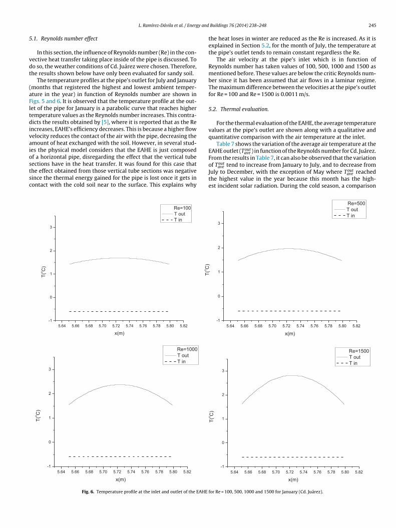
.1. Reynolds number effect
In this section, the influence of Reynolds number (Re) in the con-ective heat transfer taking place inside of the pipe is discussed. Too so, the weather conditions of Cd. Juárez were chosen. Therefore,he results shown below have only been evaluated for sandy soil.
The temperature profiles at the pipe’s outlet for July and Januarymonths that registered the highest and lowest ambient temper-ture in the year) in function of Reynolds number are shown inigs. 5 and 6. It is observed that the temperature profile at the out-et of the pipe for January is a parabolic curve that reaches higheremperature values as the Reynolds number increases. This contra-icts the results obtained by [5], where it is reported that as the Re
ncreases, EAHE’s efficiency decreases. This is because a higher flowelocity reduces the contact of the air with the pipe, decreasing themount of heat exchanged with the soil. However, in several stud-es the physical model considers that the EAHE is just composedf a horizontal pipe, disregarding the effect that the vertical tube
ections have in the heat transfer. It was found for this case thathe effect obtained from those vertical tube sections was negativeince the thermal energy gained for the pipe is lost once it gets inontact with the cold soil near to the surface. This explains why5.64 5.66 5.68 5.70 5.72 5.74 5.76 5.78 5.80 5.82-1
0
1
2
3
T(o C
)
x(m)
Re=10 0 T ou t T in
o
5.64 5.66 5.68 5.70 5.72 5.74 5.76 5.78 5.80 5.82-1
0
1
2
3
T(o C
)
x(m)
Re=100 0 T ou t T in
Fig. 6. Temperature profile at the inlet and outlet of the EAHE
Buildings 76 (2014) 238–248 245
the heat loses in winter are reduced as the Re is increased. As it isexplained in Section 5.2, for the month of July, the temperature atthe pipe’s outlet tends to remain constant regardless the Re.
The air velocity at the pipe’s inlet which is in function ofReynolds number has taken values of 100, 500, 1000 and 1500 asmentioned before. These values are below the critic Reynolds num-ber since it has been assumed that air flows in a laminar regime.The maximum difference between the velocities at the pipe’s outletfor Re = 100 and Re = 1500 is 0.0011 m/s.
5.2. Thermal evaluation.
For the thermal evaluation of the EAHE, the average temperaturevalues at the pipe’s outlet are shown along with a qualitative andquantitative comparison with the air temperature at the inlet.
Table 7 shows the variation of the average air temperature at theEAHE outlet (Tout
ave ) in function of the Reynolds number for Cd. Juárez.From the results in Table 7, it can also be observed that the variation
of Toutave tend to increase from January to July, and to decrease fromJuly to December, with the exception of May where Tout
ave reachedthe highest value in the year because this month has the high-est incident solar radiation. During the cold season, a comparison
5.64 5.66 5.68 5.70 5.72 5.74 5.76 5.78 5.80 5.82-1
0
1
2
3
T(C
)
x(m)
Re=500 T ou t T in
5.64 5.66 5.68 5.70 5.72 5.74 5.76 5.78 5.80 5.82-1
0
1
2
3
T(o C
)
x(m)
Re=150 0 T ou t T in
for Re = 100, 500, 1000 and 1500 for January (Cd. Juárez).

246 L. Ramírez-Dávila et al. / Energy and Buildings 76 (2014) 238–248
il for: a) January and b) May.
bcbflfttttsawtJtdaf
CeOTtttbppb
aRirtb4pEmJctitm
Table 8Inlet and outlet average temperatures (◦C) in function of Reynolds number for a year(Mérida).
Month Inlet temperature Outlet average temperature Toutave
Re = 100 Re = 500 Re = 1000 Re = 1500
Jan 10.1 12.5 12.7 13.0 13.3Feb 12.0 15.4 15.5 15.7 15.9Mar 14.3 17 17.1 17.3 17.5Apr 39.6 38.7 38.5 38.2 37.9May 41.2 43.4 43.1 42.6 42.1Jun 38.2 43.2 42.8 42.3 41.7Jul 38.4 39.9 39.6 39.3 38.9Aug 37.0 37.5 37.3 37 36.6Sep 36.3 36.1 35.8 35.5 35.2Oct 16.8 21.6 21.6 21.6 21.6
Re = 1500. The results in the table demonstrate that the use of EAHEis appropriate for heating or cooling in locations with extreme andmoderate climates, and not for humid hot climates.
Table 9Average temperature difference (◦C) between the outlet and inlet temperature forRe = 1500 for Cd. Juárez, México City and Mérida.
Month �Tave = Toutave − Tinlet
ave
Cd. Juárez México city Mérida
Jan 1.8 3.7 3.2Feb 2.1 2.1 3.9Mar 0.8 1.5 3.2Apr −5.2 −5.4 −1.7May −4.0 −3.5 0.9Jun −9.5 −3.9 3.5Jul −8.0 −2.3 0.5Aug −6.9 −2 −0.4
Fig. 7. Isotherms in so
etween the Toutave obtained with Re = 100 and with Re = 1500, indi-
ates an average difference of 19%. For heating purposes, the EAHEehaved better with higher Re; a higher velocity does not let theuid stay long enough in contact with the cold soil near the sur-
ace, what diminishes the loss of heat. In this city, the increase of airemperature provided by the EAHE averaged 2.1 ◦C. In December,he EAHE was able increase the air temperature up to 3.7 ◦C abovehe inlet temperature. On the other hand, during warm months,he Reynolds number did not have a significant influence on Tout
aveince the temperature variations in the soil are small. The EAHE had
more important contribution for cooling than for heating, in allarm months (from April to September) the EAHE highly decreased
he temperature. The reductions of temperature averaged 6.6 ◦C. Inune, the EAHE provided the maximum cooling effect; it reducedhe air temperature up to 9.7 ◦C. As can be seen in Fig. 7, the EAHEoes not require to be buried in great depths to work appropri-tely, after 2 m depth the temperature of the soil remains constantor summer and winter.
Fig. 8 presents Toutave in function of Reynolds number for Mexico
ity. For all months and Reynolds numbers, the EAHE behaves asxpected; the Tout
ave increased during the cold months (Jan–Mar,ct–Dec) and the Tout
ave decreased during the hot months (Apr–Sep).he Reynolds number has a small influence on Tout
ave for all months;he maximum variation of temperature was 0.7 ◦C corresponding tohe cold season. In the case of cold months, the EAHE increased theemperature between 1.5 and 3.7 ◦C with Re = 1500, and increased itetween 0.9 and 3.1 ◦C with Re = 100. On the other hand, for coolingurposes the EAHE worked better. The EAHE decreased the tem-erature between 1.9 and 5.4 ◦C with Re = 1500, and decreased itetween 1.6 and 5.4 ◦C with Re = 100.
For the case of Mérida, Table 8 presents the average air temper-ture at the outlet of the EAHE (Tout
ave ) during the year as function ofeynolds number. The EAHE achieved its objective for all months
n cold season (Jan–Mar and Oct–Dec); it was able to increase Toutave
egardless of the Reynolds number. The maximum variation of Toutave
owards Re was 0.8 ◦C for this season. The heating effect providedy the EAHE ranged from 3 to 4.8 ◦C with Re = 1500, and from 2.4 to.8 ◦C with Re = 100. Unlike its behavior for heating, the EAHE had aoor performance for cooling in this city. During the hot season, theAHE decreased Tout
ave only in 3 months (Apr, Aug and Sep), the maxi-um decrease was just 1.7 ◦C for April. For the other 3 months (May,
un and Jul) the EAHE increased Toutave . This behavior depends on the
ombination of the different parameters involved in the EAHE sys-
em (climatic conditions, soil thermal inertia, the considerationsn the physical and mathematical model, etc.). From the combina-ion of the parameters, the relative humidity (RH) is the one thatainly affects Toutave . The city of Mérida has relative humidity values
Nov 14.2 16.7 16.9 17.0 17,2Dec 12.3 16.4 16.5 16.7 16.8
greater than 60% during all the year, which causes an incrementof the soil temperature. Therefore, by increasing the soil temper-ature, the fluid toward the outlet of the EAHE significantly raisesits temperature. Then, to avoid the undesirable gains of heat, it isrecommended to insulate the vertical section at the outlet of theEAHE. This modification will be analyzed in a future work.
Finally, Table 9 presents the temperature difference (�Tave)between the outlet (Tout
ave ) and the inlet (Tinletave ) of the EAHE for the
three selected cities during the year. These values are given for
Sep −6.2 −1.9 −1.1Oct 2.5 1.9 4.8Nov 2.1 3.5 3Dec 3.7 3.5 4.5

L. Ramírez-Dávila et al. / Energy and Buildings 76 (2014) 238–248 247
in fun
6
ic
feTwtotltai
rm6tp
ft
Fig. 8. Inlet and outlet average temperatures (◦C)
. Conclusions
In this work the numerical analysis for the thermal performancen a two-dimensional EAHE is presented. From the results we canonclude the following:
For Cd. Juárez, it was observed, that comparing the Toutave obtained
or Re = 100 and Re = 1500 during winter season, an average differ-nce of 19% was obtained, which tends to increase along with Re.his is because a higher velocity in the flow reduces the interactionith the cold soil near the surface, decreasing the energy loss. On
he other hand, during the hot season, it was shown that an increasef 26.63% in the incident radiation on the soil surface can increasehe Tout
ave in 13.98%. Therefore, in order to avoid undesirable gain oross of heat, it is recommended to insulate the vertical section ofhe outlet pipe. It was also shown that the higher temperature vari-tions are located within the first 2 m depth in the soil, therefore,t is not necessary to bury the pipe to greater depths.
Also, it was observed that for Cd. Juárez and México city, resultseveal that the thermal performance of the EAHE is better in sum-er than in winter, decreasing the air temperature in an average of
.6 and 3.2 ◦C for summer and increasing it in 2.1 and 2.7 ◦C for win-er, respectively. By contrast for Mérida EAHE had its best thermal
erformance in winter, increasing the air temperature in 3.8 ◦C.In general, it is concluded that the use of EAHEs is appropriateor heating or cooling of buildings in lands of extreme and moderateemperatures where the thermal inertia effect in soil is higher.
ction of Reynolds number for a year (México city).
Acknowledgement
The authors are grateful to the Consejo Nacional de Ciencia yTecnología (CONACYT), whose financial support made this workpossible.
References
[1] H. Carslaw, J. Jaeger, Conduction of Heat in Solids, Oxford at the Claredon Press,1959.
[2] R. Cichota, E.A. Elias, Quirijn de Jong van Lier, Testing a finite-difference modelfor soil heat transfer by comparing numerical and analytical solutions, Envi-ronmental Modeling 19 (2004) 495–506.
[3] M. De Paepe, A. Janssens, Thermo-hydraulic design of earth-air heat exchang-ers, Energy and Buildings 35 (2003) 389–397.
[4] C. Gauthier, M. Lacroix, H. Bernier, Numerical simulation of soil heat exchanger-storage system for greenhouses, Solar Energy 60 (1997) 333–346.
[5] G. Mihalakakou, M. Santamouris, D. Asimakopoulos, Modelling the thermalperformance of earth-to-air heat exchangers, Solar Energy 53 (1994) 301–305.
[6] G. Mihalakakou, M. Santamouris, D. Asimakopoulos, N. Papanikolau, Impactof ground cover on the efficiencies of earth-to-air heat exchangers, AppliedEnergy 48 (1994) 19–32.
[7] G. Mihalakakou, M. Santamouris, D. Asimakopoulos, On the application of theenergy balance equation to predict ground temperature, Solar Energy 60 (1997)181–190.
[8] P. Tittelein, G. Achard, E. Wurtz, Modeling earth-to-air heat exchanger behav-
ior with the convolutive response factors method, Applied Energy 86 (2009)1683–1691.[9] S. Thiers, B. Peuportier, Thermal and environmental assessment of a passivebuilding equipped with an earth-to-air heat exchanger in France, Solar Energy82 (2008) 820–831.

2 y and
[
[
[
[
[
[
[
[
[
[
[
[
[
[
[
[
[
[
[
[
48 L. Ramírez-Dávila et al. / Energ
10] M.M. Salah El-Din, On the heat flow into the ground, Renewable Energy 18(1999) 473–490.
11] V. Badescu, Simple and accurate model for the ground heat exchanger of apassive house, Renewable Energy 32 (2007) 845–855.
12] M. Cucumo, S. Cucumo, L. Montoro, A. Vulcano, A one-dimensional transientanalytical model for earth-to-air heat exchangers, taking into account conden-sation phenomena and thermal perturbation from the upper free surface as wellas around the buried pipes, International Journal of Heat and Mass Transfer 51(2008) 506–516.
13] P. Hollmuller, B. Lachal, Cooling and preheating with buried pipe systems:monitoring, simulation and economic aspects, Energy and Buildings 33 (2001)509–518.
14] V.A.F. Costa, Thermodinamic analysis of building heating or cooling using thesoil as heat reservoir, Heat and Mass Transfer 49 (2006) 4152–4160.
15] A. Benazza, E. Blanco, M. Aichouba, José Luis Río, S. Laouedj, Numerical investi-gation of horizontal ground coupled heat exchanger, Energy Procedia 6 (2011)29–35.
16] M. Bojic, N. Trifunovic, G. Papadakis, S. Kyritsis, Numerical simulation, technicaland economic evaluation of air-to-earth heat exchanger coupled to a building,Energy 22 (1997) 1151–1158.
17] G. Florides, P. Christodoulides, P. Pouloupatis, An analysis of heat flowthrough a borehole heat exchanger validated model, Applied Energy 92 (2012)523–533.
18] R. Misra, V. Bansal, G. Das Agrawal, J. Mathur, T.K. Aseri, CFD analysis based
parametric study of derating factor for earth air tunnel heat exchanger, AppliedEnergy 103 (2012) 266–277.19] M. Santamouris, G. Mihalakakou, C.A. Balaras, J.O. Lewis, M. Vallindras, A.Argiriou, Energy conservation in greenhouses with buried pipes, Energy 21(1995) 353–360.
[
[
Buildings 76 (2014) 238–248
20] M. Santamouris, G. Mihalakakou, C.A. Balaras, A. Argiriou, D.N. Asimakopoulos,On the performance of buildings coupled with earth to air heat exchangers,Solar Energy 54 (1995) 375–380.
21] Su.H. Xiao-Bing Liu, Jing-Yu Mu, A numerical model of a deeply buried air-earth-tunnel heat exchanger, Energy and Buildings 48 (2012) 233–239.
22] G. Yoon, H. Tanaka, M. Okimiya, Study on the design procedure for a multi-cool/heat tube system, Solar Energy 83 (2009) 1415–1424.
23] A. Sehli, A. Hasni, M. Tamali, The potential of earth-air heat exchanger forlow energy cooling of buildings in South Algeria, Energy Procedia 18 (2012)496–506.
24] M. Bojic, G. Papadakis, S. Kyritsis, Energy from a two-pipe, earth-to-air heatexchanger, Energy 24 (1999) 519–523.
25] P. Roth, A. Georgiev, A. Busso, E. Barraza, First in situ determination of groundand borehole thermal properties in Latin America, Renewable Energy 29 (2004)1947–1963.
26] S. Amara, B. Nordell, B. Benyoucef, Using fouggara for heating and coolingbuildings in Sahara, Energy Procedia 6 (2011) 55–64.
27] O. Ozgener, L. Ozgener, Determining the optimal design of a closed loop earth toair heat exchager for heating by using exergoeconomics, Energy and Buildings43 (2011) 960–965.
28] S.V. Patankar, Numerical Heat Transfer and Fluid Flow, Hemisphere Publishing,Washington, 1980.
29] J. Van Doormaal, G. Raithby, Enhancements of the SIMPLE method forpredicting incompressible fluid flow, Numerical Heat Transfer 7 (1984)
147–163.30] A.A. Mohamad, I. Sezai, Natural convection in C-shaped thermosyphon, Numer-ical Heat Transfer, Part A 32 (1997) 311–323.
31] P. Nielsen, Specification of a two dimensional test case, Energy Conservation inBuildings and Community System, Annex 20, Denmark, 1990.