Instructions for use

Title Interannual and latitudinal changes in zooplankton abundance, biomass and size composition along a central NorthPacific transect during summer : analyses with an Optical Plankton Counter

Author(s) Fukuda, Jumpei; Yamaguchi, Atsushi; Matsuno, Kohei; Imai, Ichiro

Citation Plankton & benthos research, 7(2): 64-74

Issue Date 2012-05

Doc URL http://hdl.handle.net/2115/52334

Rights © 2012 Plankton Society of Japan

Type article

File Information 3-Fukuda et al. 2012.pdf

Hokkaido University Collection of Scholarly and Academic Papers : HUSCAP

Plankton Benthos Res 7(2): 64–74, 2012

Interannual and latitudinal changes in zooplankton abundance, biomass and size composition along a central North Pacific transect during summer: analyses with an Optical Plankton Counter

JUMPEI FUKUDA, ATSUSHI YAMAGUCHI*, KOHEI MATSUNO & ICHIRO IMAI

Laboratory of Marine Biology, Graduate School of Fisheries Science, Hokkaido University, 3–1–1 Minatomachi, Hakodate, Hokkaido 041–8611, Japan

Received 20 July 2011; Accepted 15 March 2012

Abstract: To evaluate zooplankton interannual and latitudinal changes, Optical Plankton Counter analyses were made on preserved net zooplankton samples collected by NORPAC net from 0–150 m at 35°N–51°N stations along 180° in the central North Pacific during early–mid June 1981–2000. The mean numerical abundance of total zoo-plankton for the 20 years varied latitudinally from 19,200 to 84,300 ind. m－2 but the differences between the three oceanic domains were not significant. However, highly significant latitudinal changes were observed in the mean zooplankton biomass, which ranged from 1.44 to 13.2 mg dry mass m－2 with higher values in the Transitional Do-main (TR) than in the Subarctic and Subtropical Domains. The high biomass in the TR was caused by the dominance of large-sized zooplankton with equivalent spherical diameters (ESD) of 2–4 mm, regarded to consist mainly of Neo-calanus spp. C5. Both the slope and intercept of the Normalized Biomass Size Spectrum also showed significant lati-tudinal changes with a moderate slope and low intercept in the TR due to the dominance of large zooplankton with 2–4 mm ESD in biomass. In contrast to these large latitudinal changes, only limited interannual variations were ob-served for zooplankton abundance and biomass in the central North Pacific during the study period.

Key words: NBSS, Neocalanus, OPC, size, Transitional Domain

Introduction

In the marine ecosystem, zooplankton has a vital role, acting as a biological pump connecting primary production and fish production. In the North Pacific, climate regime shifts caused by the Pacific Decadal Oscillation have been reported, and these regime shifts are known to have a great effect on marine ecosystems (McFarlane et al. 2000, Over-land et al. 2002, PICES 2004). Long-term changes in zoo-plankton abundance, biomass and community structure have been reported at Ocean Station P (Mackas et al. 2007) and CalCOFI (Clarke & Dottori 2007) in the eastern North Pacific, and Oyashio region in the western North Pa-cific (Chiba et al. 2006). Information on long-term changes in zooplankton communities in the central North Pacific include annual and regional changes in biomass reported

by Sugimoto & Tadokoro (1997, 1998), annual changes in biomass reported by Shiomoto et al. (1997) and annual changes in abundance and body size of Neocalanus cope-pods reported by Kobari et al. (2003a).

In addition to interannual changes in zooplankton, their numerical abundance, biomass and community structure are known to also change with latitude (Odate K 1994, Saito et al. 2011). Zooplankton biomass in the oceanic sub-arctic Pacific is strongly linked to the abundances of large copepods Neocalanus spp. (Kobari et al. 2003a). Latitudi-nal differences in the developmental timing of Neocalanus spp. have also been reported (Batten et al. 2003). During spring to summer, latitudinal changes in zooplankton abundance, biomass and community structure in the North Pacific have been reported for the western (165°E) and eastern (165°W) regions (Matsuno & Yamaguchi 2010) and the western (155°E) region (Yokoi et al. 2008). Common to these studies, the highest biomass and lowest abundances have been reported for the transitional region (TR) (Yokoi

* Corresponding author: Atsushi Yamaguchi; E-mail, a-yama@fish.hokudai.ac.jp

Plankton & Benthos Research

© The Plankton Society of Japan

OPC analysis on zooplankton community 65

et al. 2008, Matsuno & Yamaguchi 2010). It is not known whether this pattern is common across the whole North Pa-cific, as there is little information on zooplankton commu-nity structure throughout the region.

Information on the size spectra of zooplankton biomass is important from the viewpoint of both fisheries (as a food source for fish) and biogeochemical cycling (as a mediator of vertical flux). However, little information is available on zooplankton size spectra. This is partly due to the time and skill required to perform microscopic analysis and taxo-nomic identification, respectively. In most cases, zooplank-ton samples are only analyzed for biomasses (cf. Postel et al. 2000). Advancements in zooplankton analysis have been made using an Optical Plankton Counter (OPC) (Her-man 1988, 1992), which can measure zooplankton sizes ac-curately and rapidly. Data produced by OPC analysis are easily applicable to Normalized Biomass Size Spectra (NBSS), which can evaluate the characteristics of aquatic ecosystem structure. A combination of OPC and NBSS analyses has been conducted on various aquatic ecosys-tems (Zhou & Huntley 1997, Herman & Harvey 2006, Basedow et al. 2010).

In the present study, OPC analyses were done on net zooplankton samples collected from 35°N–51°N along 180° in the central North Pacific during early–mid June 1981–2000. Using these samples, we evaluated interannual and latitudinal changes in zooplankton abundance, biomass and size composition. NBSS were also constructed from the OPC data, and were analyzed to understand possible interannual and latitudinal changes.

Materials and Methods

Field sampling

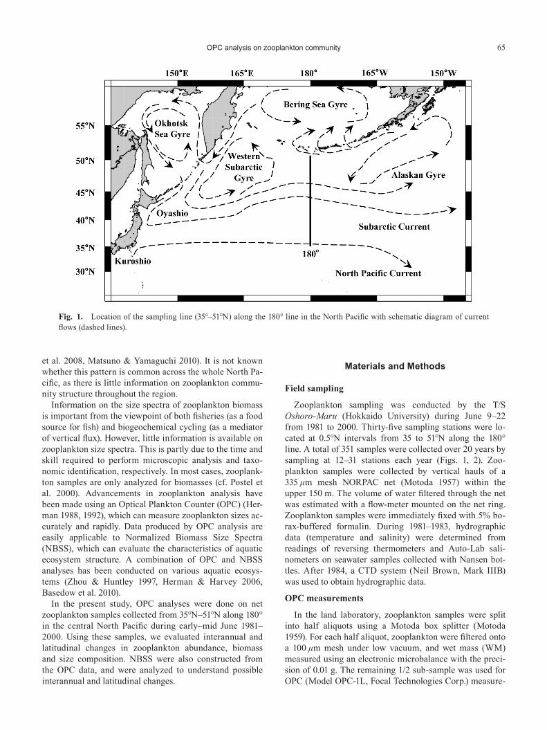
Zooplankton sampling was conducted by the T/S Oshoro-Maru (Hokkaido University) during June 9–22 from 1981 to 2000. Thirty-five sampling stations were lo-cated at 0.5°N intervals from 35 to 51°N along the 180° line. A total of 351 samples were collected over 20 years by sampling at 12–31 stations each year (Figs. 1, 2). Zoo-plankton samples were collected by vertical hauls of a 335 μm mesh NORPAC net (Motoda 1957) within the upper 150 m. The volume of water filtered through the net was estimated with a flow-meter mounted on the net ring. Zooplankton samples were immediately fixed with 5% bo-rax-buffered formalin. During 1981–1983, hydrographic data (temperature and salinity) were determined from readings of reversing thermometers and Auto-Lab sali-nometers on seawater samples collected with Nansen bot-tles. After 1984, a CTD system (Neil Brown, Mark IIIB) was used to obtain hydrographic data.

OPC measurements

In the land laboratory, zooplankton samples were split into half aliquots using a Motoda box splitter (Motoda 1959). For each half aliquot, zooplankton were filtered onto a 100 μm mesh under low vacuum, and wet mass (WM) measured using an electronic microbalance with the preci-sion of 0.01 g. The remaining 1/2 sub-sample was used for OPC (Model OPC-1L, Focal Technologies Corp.) measure-

Fig. 1. Location of the sampling line (35°–51°N) along the 180° line in the North Pacific with schematic diagram of current flows (dashed lines).

66 J. Fukuda et al.

ments with the aid of a flow-through system (Beaulieu et al. 1999, Yokoi et al. 2008). OPC measurements were made with conditions of low flow rate (<10 L min－1) and low par-ticle density (<10 counts sec－1) without staining (Yokoi et al. 2008). While samplings were conducted from 1981 to 2000, samples that had been sorted with Neocalanus spp. and chaetognaths removed for the purpose of other studies (Nishiuchi et al. 1997, Kobari et al. 2003a) (whole samples in 1987 and 1992 and a portion of the 1996 samples) as well as 41 samples dominated by salps were not used for the OPC analyses.

Abundance and biomass

Numerical abundance per square meter (N, ind. m－2) for each of the 4,096 equivalent spherical diameter (ESD) size categories was calculated using the following equation:

150nN

s F×

=×

where n is the number of particles (=zooplankton ind.), s is the split factor of each sample, F is the filtered volume of the net (m3), and 150 is the depth of the vertical net tow (m). WM of the zooplankton community in the 4,096 size categories was calculated from ESD data by assuming the relative density of zooplankton to be equal to seawater (=1

mg mm－3). During the course of OPC analysis, dominant plankton in the samples were checked by eye before mea-surement, and scored into three categories, viz. non-gelati-nous zooplankton-dominated, phytoplankton-dominated and gelatinous zooplankton-dominated samples. For each category, correlation coefficients between OPC-derived and directly measured WMs were obtained. Using these coefficients, zooplankton WM was calculated from OPC-derived masses and then converted to dry mass (DM) as-suming that the water content of zooplankton was 90% (DM=0.1×WM), which is the mean water content of zoo-plankton at 0–1,000 m from subarctic to subtropical areas in the North Pacific Ocean (Yamaguchi et al. 2005). Anal-yses on zooplankton biomass were made for six size classes viz. ≤1, >1 and ≤2, >2 and ≤3, >3 and ≤4, >4 and ≤5, and >5 mm ESD, which are referred to simply as 0–1, 1–2, 2–3, 3–4, 4–5, and >5 mm ESD, respectively.

Data processing

Zooplankton sampling in this study was conducted both day and night. In this region, day-night differences in abundance have been reported for copepod Metridia paci-fica C6F (Saito et al. 2011). However, significant day-night differences in OPC-derived total plankton abundance and biomass were not detected in any of the regions (Matsuno & Yamaguchi 2010). This may partly be because the broader size range surveyable using the OPC (0.250–20 mm) may mask the day-night differences that were ob-served for a relatively narrower size range. Because the re-gional differences in abundance were greater than the day-night differences in this region (Matsuno & Yamaguchi 2010), we made no conversion according to the diel regime.

From the OPC data, NBSS was calculated following the procedure of Zhou (2006). First, zooplankton DM (B, mg DM m－3) was averaged for every 100 μm ESD size class. To calculate the X axis of NBSS (log10 zooplankton weight, μg DM ind.－1), B was multiplied by 1,000 to change units (μg DM m－3), divided by the abundance of each size class (ind. m－3) and then log scaled. To calculate the Y axis of NBSS (log10 zooplankton biomass [μg DM L－1]/⊿weight [μg DM]), B was divided by the interval of DM (⊿weight: μg DM) and log scaled. Based on these data, an NBSS lin-ear model (Y=aX+b) was calculated, where a and b are the slope and intercept of the NBSS, respectively.

To evaluate interannual changes, the mean and standard deviation at each station (30′ each in latitude) were calcu-lated for integrated mean temperature and salinity (0–150 m), zooplankton abundance, biomass (total and each ESD category), and slope and intercept of the NBSS. For each parameter, the anomaly from the mean was calculated for each year.

The Northern boundary of the Transition Domain (NTD) was determined based on the position of the 4°C isothermal line (Favorite et al. 1976). The position of the Subarctic Boundary (SB) was also determined from the position of the 34 isohaline line (Favorite et al. 1976). From

Fig. 2. Location of sampling stations along the 180° line in the central North Pacific during June of 1981–2000. Northern bound-ary of the Transition Domain (NTD) and Subarctic Boundary (SB) are marked with horizontal dashed lines, by which Subarc-tic (SA), Transitional (TR) and Subtropical (ST) Domains are separated. The two climate regime shifts at 1988/89 and 1997/98 reported are shown with vertical dashed lines.

OPC analysis on zooplankton community 67

these two boundaries, three regions were defined: north of the NTD was defined as the Subarctic Domain (SA), the re-gion between the NTD and the SB was the TR, and south of the SB was the Subtropical Domain (ST) (Favorite et al. 1976). During the study period (1980–2000), there were two reported climatic regime shifts (1988/89 and 1997/98) in the North Pacific (PICES 2004). Based on this informa-tion, the sampling period was separated into three regimes: 1981–1988, 1989–1997 and 1998–2000.

To evaluate interannual and latitudinal changes, one-way ANOVA and Fisher’s PLSD were used to test differ-ences between the three spatial (SA, TR and ST) and tem-poral regimes (1981–1988, 1989–1997 and 1998–2000) of integrated mean temperature and salinity, zooplankton abundance, biomass, slope and intercept of the NBSS.

Results

Hydrography

The mean of the integrated mean temperature of the top 150-m of the water column over 20 years varied latitudi-nally between 4.1 and 15.6°C, but exhibited limited vari-ability in the SA (Fig. 3a). Greater latitudinal changes were

observed in the TR and the ST, with higher temperatures associated with lower latitudes. The anomaly ranged be-tween －2.65 and 1.97°C, and was higher during 1987–1997.

The mean of the integrated mean salinity ranged be-tween 33.01 and 34.53 and exhibited limited latitudinal change in the SA and ST (Fig. 3b). Large latitudinal changes were observed in the TR, with increased salinity associated with lower latitudes. The anomaly ranged be-tween －0.30 and 0.82, and was higher during 1989–1997 in the TR and ST, while it was higher during 1981–1988 in the SA.

OPC calibration

OPC-derived WMs in all samples were significantly correlated with directly measured WMs with a conversion factor of 1.178 (Fig. 4a). This factor varied with the domi-nant taxonomic component of the samples, i.e. higher (1.397 times) for samples dominated by non-gelatinous zooplankton consisting mainly of copepods and chaeto-gnaths but lower for samples dominated by gelatinous zoo-plankton (0.702) and phytoplankton (0.796) (Fig. 4b–d).

Abundance and biomass

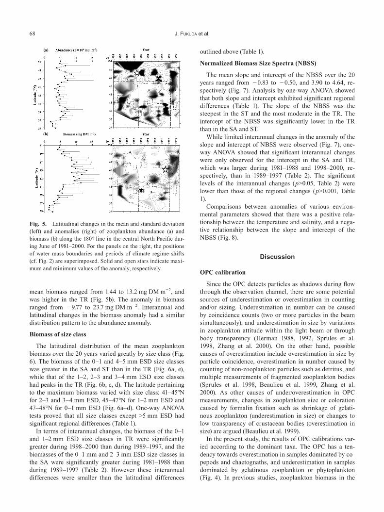
The mean zooplankton abundance over the 20 years ranged from 19,200 to 84,300 ind. m－2, and varied little by latitude (Fig. 5a). The anomaly ranged from －61,800 to 248,500 ind. m－2, with large variability in all regions. The

Fig. 3. Latitudinal changes in the mean and standard deviation (left) and anomalies (right) of integrated mean temperature (a) and salinity (b) of the 0–150 m water column along the 180° line in the central North Pacific during June of 1981–2000. For the panels on the right, the positions of water mass boundaries and periods of climate regime shifts (cf. Fig. 2) are superimposed. Solid and open stars indicate maximum and minimum values of the anomaly, respectively.

Fig. 4. Comparison between OPC-derived (Y) and directly measured wet masses (X) for all (a), non-gelatinous zooplankton-dominated (b), gelatinous zooplankton-dominated (c) and phyto-plankton-dominated (d) samples. Dashed lines indicate positions of Y=X.

68 J. Fukuda et al.

mean biomass ranged from 1.44 to 13.2 mg DM m－2, and was higher in the TR (Fig. 5b). The anomaly in biomass ranged from －9.77 to 23.7 mg DM m－2. Interannual and latitudinal changes in the biomass anomaly had a similar distribution pattern to the abundance anomaly.

Biomass of size class

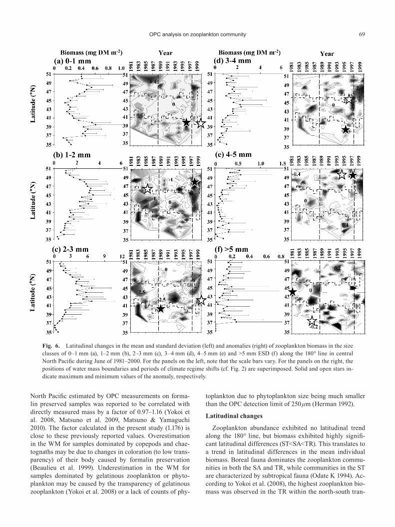
The latitudinal distribution of the mean zooplankton biomass over the 20 years varied greatly by size class (Fig. 6). The biomass of the 0–1 and 4–5 mm ESD size classes was greater in the SA and ST than in the TR (Fig. 6a, e), while that of the 1–2, 2–3 and 3–4 mm ESD size classes had peaks in the TR (Fig. 6b, c, d). The latitude pertaining to the maximum biomass varied with size class: 41–45°N for 2–3 and 3–4 mm ESD, 45–47°N for 1–2 mm ESD and 47–48°N for 0–1 mm ESD (Fig. 6a–d). One-way ANOVA tests proved that all size classes except >5 mm ESD had significant regional differences (Table 1).

In terms of interannual changes, the biomass of the 0–1 and 1–2 mm ESD size classes in TR were significantly greater during 1998–2000 than during 1989–1997, and the biomasses of the 0–1 mm and 2–3 mm ESD size classes in the SA were significantly greater during 1981–1988 than during 1989–1997 (Table 2). However these interannual differences were smaller than the latitudinal differences

outlined above (Table 1).

Normalized Biomass Size Spectra (NBSS)

The mean slope and intercept of the NBSS over the 20 years ranged from －0.83 to －0.50, and 3.90 to 4.64, re-spectively (Fig. 7). Analysis by one-way ANOVA showed that both slope and intercept exhibited significant regional differences (Table 1). The slope of the NBSS was the steepest in the ST and the most moderate in the TR. The intercept of the NBSS was significantly lower in the TR than in the SA and ST.

While limited interannual changes in the anomaly of the slope and intercept of NBSS were observed (Fig. 7), one-way ANOVA showed that significant interannual changes were only observed for the intercept in the SA and TR, which was larger during 1981–1988 and 1998–2000, re-spectively, than in 1989–1997 (Table 2). The significant levels of the interannual changes (p>0.05, Table 2) were lower than those of the regional changes (p>0.001, Table 1).

Comparisons between anomalies of various environ-mental parameters showed that there was a positive rela-tionship between the temperature and salinity, and a nega-tive relationship between the slope and intercept of the NBSS (Fig. 8).

Discussion

OPC calibration

Since the OPC detects particles as shadows during flow through the observation channel, there are some potential sources of underestimation or overestimation in counting and/or sizing. Underestimation in number can be caused by coincidence counts (two or more particles in the beam simultaneously), and underestimation in size by variations in zooplankton attitude within the light beam or through body transparency (Herman 1988, 1992, Sprules et al. 1998, Zhang et al. 2000). On the other hand, possible causes of overestimation include overestimation in size by particle coincidence, overestimation in number caused by counting of non-zooplankton particles such as detritus, and multiple measurements of fragmented zooplankton bodies (Sprules et al. 1998, Beaulieu et al. 1999, Zhang et al. 2000). As other causes of under/overestimation in OPC measurements, changes in zooplankton size or coloration caused by formalin fixation such as shrinkage of gelati-nous zooplankton (underestimation in size) or changes to low transparency of crustacean bodies (overestimation in size) are argued (Beaulieu et al. 1999).

In the present study, the results of OPC calibrations var-ied according to the dominant taxa. The OPC has a ten-dency towards overestimation in samples dominated by co-pepods and chaetognaths, and underestimation in samples dominated by gelatinous zooplankton or phytoplankton (Fig. 4). In previous studies, zooplankton biomass in the

Fig. 5. Latitudinal changes in the mean and standard deviation (left) and anomalies (right) of zooplankton abundance (a) and biomass (b) along the 180° line in the central North Pacific dur-ing June of 1981–2000. For the panels on the right, the positions of water mass boundaries and periods of climate regime shifts (cf. Fig. 2) are superimposed. Solid and open stars indicate maxi-mum and minimum values of the anomaly, respectively.

OPC analysis on zooplankton community 69

North Pacific estimated by OPC measurements on forma-lin preserved samples was reported to be correlated with directly measured mass by a factor of 0.97–1.16 (Yokoi et al. 2008, Matsuno et al. 2009, Matsuno & Yamaguchi 2010). The factor calculated in the present study (1.176) is close to these previously reported values. Overestimation in the WM for samples dominated by copepods and chae-tognaths may be due to changes in coloration (to low trans-parency) of their body caused by formalin preservation (Beaulieu et al. 1999). Underestimation in the WM for samples dominated by gelatinous zooplankton or phyto-plankton may be caused by the transparency of gelatinous zooplankton (Yokoi et al. 2008) or a lack of counts of phy-

toplankton due to phytoplankton size being much smaller than the OPC detection limit of 250 μm (Herman 1992).

Latitudinal changes

Zooplankton abundance exhibited no latitudinal trend along the 180° line, but biomass exhibited highly signifi-cant latitudinal differences (ST<SA<TR). This translates to a trend in latitudinal differences in the mean individual biomass. Boreal fauna dominates the zooplankton commu-nities in both the SA and TR, while communities in the ST are characterized by subtropical fauna (Odate K 1994). Ac-cording to Yokoi et al. (2008), the highest zooplankton bio-mass was observed in the TR within the north-south tran-

Fig. 6. Latitudinal changes in the mean and standard deviation (left) and anomalies (right) of zooplankton biomass in the size classes of 0–1 mm (a), 1–2 mm (b), 2–3 mm (c), 3–4 mm (d), 4–5 mm (e) and >5 mm ESD (f) along the 180° line in central North Pacific during June of 1981–2000. For the panels on the left, note that the scale bars vary. For the panels on the right, the positions of water mass boundaries and periods of climate regime shifts (cf. Fig. 2) are superimposed. Solid and open stars in-dicate maximum and minimum values of the anomaly, respectively.

70 J. Fukuda et al.

sect (155°E) in the western North Pacific during May to early June. They indicated that the 2–3 mm ESD size class in the TR corresponds to the size of the copepodid fifth stage (C5) of the boreal copepod N. plumchrus. Also for the central North Pacific, abundances of Neocalanus spp. (N. cristatus, N. flemingeri and N. plumchrus) C5 are known to be greater in the TR than in the SA and ST (Ko-bari et al. 2003a). In the present study, biomasses in size classes of 1–2 mm, 2–3 mm, and 3–4 mm ESD were greater in the order of ST<SA<TR. The same latitudinal trend in total zooplankton biomass (ST<SA<TR) caused by 2–4 mm ESD size class has been reported for north-south transects in the western (165°E) and eastern North Pacific (165°W) during summer (June to August) (Matsuno & Ya-maguchi 2010).

Thus, the latitudinal changes in zooplankton biomass (ST<SA<TR) are common throughout the western, central and eastern North Pacific, and are caused by the domi-nance of Neocalanus spp. C5 in TR, belonging to the 2–4 mm ESD size class (Kobari et al. 2003a, Yokoi et al. 2008, Matsuno & Yamaguchi 2010, Saito et al. 2011). To explain the cause of the dominance of N. plumchrus C5 in the TR, Batten et al. (2003) reported that the growth of N. plum-

chrus in the TR was five weeks faster than that in the SA, and was accelerated by higher temperatures in the TR. However, it should be noted that these reports are based on data collected during the summer (June–August). Since the surface dwelling period of Neocalanus spp. is reported to vary according to species (cf. Kobari & Ikeda 1999, 2001a, b, Tsuda et al. 1999), observations in different seasons may lead to different apparent latitudinal patterns.

While boreal copepods occurred both in the SA and TR (Odate K 1994, Saito et al. 2011), the higher temperature in the TR may induce faster development of Neocalanus spp., leading to the dominance of large-sized C5 and greater biomass in the TR (Batten et al. 2003). In the present study, the latitude pertaining to the maximum biomass varied with size class: 41–45°N for 2–3 and 3–4 mm ESD, 45–47°N for 1–2 mm ESD and 47–48°N for 0–1 mm ESD. Saito et al. (2011) suggested that the northward shift in the peak latitude of biomass comprised of smaller sized organ-isms reflected the dominance of early copepodid stages of Neocalanus spp. in higher latitudes, caused by their slower development under low temperature conditions.

The latitudinal changes in slope and intercept of the NBSS in the TR were more moderate and lower, respec-

Table 1. Summary of regional differences (SA: Subarctic, TR: Transitional and ST: Subtropical Domains) in environmental parame-ters, zooplankton abundance, biomass, slope and intercept of the NBSS. Regional differences were tested by one-way ANOVA and post hoc tests with Fisher’s PLSD. Values are mean±1sd. ***: p<0.001, NS: not significant. Any regions not connected by the same underline are significantly different (p<0.05). ESD: Equivalent Spherical Diameter.

ParameterRegion

Differences Fisher’s PLSDSA TR ST

Temperature (°C) 4.46±0.51 7.93±1.69 11.96±1.63 *** SA TR ST

Salinity 33.06±0.08 33.66±0.35 34.25±0.16 *** SA TR ST

Total abundance (1×104 ind. m－2) 6.01±4.71 4.49±2.25 5.68±3.40 NS

Total biomass (mg DM m－2) 6.72±3.99 9.87±5.69 4.52±4.39 *** ST SA TR

Biomass 0–1 mm ESD (mg DM m－2) 0.41±0.26 0.24±0.16 0.46±0.31 *** TR SA ST

Biomass 1–2 mm ESD (mg DM m－2) 2.12±1.45 2.62±1.65 1.28±1.10 *** ST SA TR

Biomass 2–3 mm ESD (mg DM m－2) 2.45±1.94 5.08±3.36 1.85±2.51 *** ST SA TR

Biomass 3–4 mm ESD (mg DM m－2) 1.22±1.27 1.71±1.65 0.70±1.05 *** ST SA TR

Biomass 4–5 mm ESD (mg DM m－2) 0.35±0.36 0.11±0.18 0.14±0.22 *** TR ST SA

Biomass >5 mm ESD (mg DM m－2) 0.14±0.16 0.10±0.26 0.10±0.22 NS

Slope of the NBSS－0.73±0.12 －0.58±0.14 －0.81±0.16 *** ST SA TR

Intercept of the NBSS 4.44±0.37 4.10±0.36 4.44±0.43 *** TR ST SA

OPC analysis on zooplankton community 71

Table 2. Comparison of environmental parameters, zooplankton abundance, biomass, slope and intercept of the NBSS between three climate regimes (R1: 1981–88, R2: 1989–1997 and R3: 1998–2000). Differences were tested by one-way ANOVA and Fisher’s PLSD. *: p<0.05, **: p<0.01, ***: p<0.001, NS: not significant. Any regimes not connected by the same underline are significantly different (p<0.05). ESD: Equivalent Spherical Diameter.

Parameter PeriodDifferences Fisher’s PLSDRegion R1 R2 R3

Temperature (°C)SA 4.366±0.371 4.576±0.562 4.049±0.245 ** R3 R1 R2TR 7.903±1.676 8.171±1.516 7.231±2.077 NSST 10.833±1.492 12.496±1.356 12.968±1.384 *** R1 R2 R3

SalinitySA 33.103±0.075 33.026±0.071 33.074±0.084 *** R2 R3 R1TR 33.703±0.286 33.716±0.352 33.376±0.339 ** R3 R1 R2ST 34.150±0.177 34.304±0.124 34.261±0.128 *** R1 R3 R2

Total abundance (1×104 ind. m－2)SA 6.672±4.278 5.562±4.866 6.264±5.612 NSTR 4.655±1.945 3.941±1.903 5.878±3.148 * R2 R1 R3ST 5.765±2.732 5.956±3.820 3.561±2.219 NS

Total biomass (mg DM m－2)SA 7.443±3.788 6.071±3.626 8.326±6.621 NSTR 9.653±4.558 9.422±5.901 11.732±6.972 NSST 5.361±5.837 4.404±3.427 1.935±1.436 NS

Biomass 0–1 mm ESD (mg DM m－2)SA 0.496±0.257 0.346±0.225 0.441±0.438 ** R2 R3 R1TR 0.249±0.153 0.194±0.107 0.351±0.258 ** R2 R1 R3ST 0.463±0.243 0.481±0.347 0.275±0.155 NS

Biomass 1–2 mm ESD (mg DM m－2)SA 2.464±1.269 1.870±1.343 2.487±2.567 NSTR 2.809±1.478 2.185±1.304 3.577±2.432 ** R2 R1 R3ST 1.444±1.330 1.296±0.975 0.468±0.285 NS

Biomass 2–3 mm ESD (mg DM m－2)SA 3.068±2.293 2.116±1.578 2.628±2.127 * R2 R3 R1TR 4.951±2.717 4.911±3.692 5.618±3.570 NSST 2.586±3.561 1.579±1.672 0.689±0.782 NS

Biomass 3–4 mm ESD (mg DM m－2)SA 0.985±1.020 1.260±1.282 2.022±1.991 NSTR 1.405±1.401 1.869±1.745 1.871±1.808 NSST 0.731±1.024 0.716±1.121 0.426±0.549 NS

Biomass 4–5 mm ESD (mg DM m－2)SA 0.295±0.294 0.353±0.372 0.529±0.471 NSTR 0089±0.134 0.105±0.112 0.192±0.353 NSST 0.089±0.130 0.185±0.264 0.067±0.068 NS

Biomass >5 mm ESD (mg DM m－2)SA 0.138±0.073 0.125±0.151 0.219±0.159 NSTR 0.128±0.327 0.077±0.208 0.128±0.250 NSST 0.038±0.075 0.146±0.277 0.010±0.029 * R3 R1 R2

Slope of the NBSSSA －0.751±0.121 －0.719±0.114 －0.736±0.109 NSTR －0.598±0.143 －0.550±0.137 －0.611±0.150 NSST －0.806±0.169 －0.814±0.162 －0.784±0.118 NS

Intercept of the NBSSSA 4.559±0.348 4.368±0.365 4.450±0.405 * R2 R3 R1TR 4.139±0.366 4.015±0.310 4.261±0.440 * R2 R1 R3ST 4.441±0.411 4.478±0.452 4.152±0.270 NS

72 J. Fukuda et al.

tively, than in the SA and ST. There was a negative rela-tionship between the slope and intercept of the NBSS. Suthers et al. (2006) noted that the slope and intercept of NBSS can exhibit three different patterns depending on the effect of bottom-up or top-down controls: i) a nutrient pulse stimulates phytoplankton, increasing the (normal-ized) biomass concentration of small zooplankton parti-cles, which is then passed on through predation to larger particles to result in the low slope and low intercept pat-tern; ii) a sustained nutrient supply increases the biomass and intercept, resulting in the high intercept pattern; iii) size-selective predation by larval and juvenile fish could steepen the slope, and their excreted nutrients could in-crease the production of smaller plankton, resulting in a steep slope and high intercept pattern. In the present study, the moderate slope and low intercept of the NBSS in the TR corresponded to case i). This pattern was caused by the high biomass value of larger size class biomass (2–3 and 3–4 mm ESD) in the TR. For the observed latitudinal changes, the biomass of 1–2, 2–3 and 3–4 mm ESD classes were higher in the order of ST<SA<TR, which was in com-mon with the slope of the NBSS. The biomass of the 0–1 mm ESD size class exhibited a reversed latitudinal pattern: TR<SA<ST. This reversed latitudinal pattern between bio-

masses of the 0–1 and 1–4 mm ESD size classes may be interpreted to be due to large zooplankton (1–4 mm ESD) feeding on smaller-sized plankton (0–1 mm ESD).

The latitudinal trend explained by predation pressure by large zooplankton increases in the order of ST<SA<TR, and was observed in the slopes of the NBSS. Large-sized zooplankton dominance in TR is due to Neocalanus spp. C5 (Kobari et al. 2003a, Saito et al. 2011). The major prey of Neocalanus spp. C5 have been reported to be phyto-plankton and microzooplankton (Nagasawa et al. 2001, Kobari et al. 2003b), though these micro-sized taxa were not quantified in this study. To confirm the latitudinal changes in predation pressure by mesozooplankton, quan-

Fig. 7. Latitudinal changes in the mean and standard deviation (left) and anomalies (right) of the slope (a) and intercept (b) of the NBSS (Y=aX+b) on mesozooplankton biomass along the 180° line in the central North Pacific during June of 1981–2000. For panels on the right, the positions of water mass boundaries and periods of climate regime shifts (cf. Fig. 2) are superimposed. Solid and open stars indicate maximum and minimum values of the anomaly, respectively.

Fig. 8. Relationships between salinity and temperature anom-alies (a) and between intercept and slope anomalies of the NBSS (b).

OPC analysis on zooplankton community 73

titative studies on the whole planktonic community along a latitudinal transect (cf. Odate T 1994) is needed in the fu-ture.

Interannual variations

The influence of climate regime shifts in the North Pa-cific is known to be greater in the east/west marginal re-gions than in the central region (PICES 2004). In the pres-ent study, both temperature and salinity showed minimal differences compared to those evident in known regime shifts. While there were slight temporal disparities be-tween temperature and salinity measurements within the same region, we should conclude that climate regime shifts may only minimally affect the hydrography of the central North Pacific.

It also should be noted that the observed duration of this study (20 years) is too short to evaluate the effects of cli-mate regime shifts on the planktonic community. For stud-ies that successfully evaluated the effects of climate change on planktonic communities, datasets were of the order of 40 years (Sugimoto & Tadokoro 1997, 1998) or 50 years (Chiba et al. 2006), while for relatively short-term observations (10–20 years), year-to-year effects such as bi-annual feeding impact of pink salmon have been evaluated (Shiomoto et al. 1997, Kobari et al. 2003a). However, a 10–20 year period is not of sufficient length to evaluate the effects of climate regime shifts on planktonic communities (Kobari et al. 2003a). Indeed, clear interannual changes were not detected in this study.

For total zooplankton abundance and biomass, only zoo-plankton abundance in the TR exhibited significant inter-annual variation, yet the statistical significance was not high (p<0.05), and biomass exhibited no significant inter-annual variation throughout the region. Chiba et al. (2006) investigated long-term changes in zooplankton abundance in the Oyashio region of the western North Pacific during March-October over a period of 50 years (1953–2002). They noted that the peak period of zooplankton abundance shifted one month earlier from June-July to May-June after the regime shift in the mid-1970s, and returned to June-July during the 1990s. The observed high zooplankton abundance in the TR of the central North Pacific during 1998–2000 could not be explained by the anomalies in temperature or salinity. The same interannual variations in zooplankton biomass (highest during 1998–2000) in the TR were observed for 0–1 mm and 1–2 mm ESD size classes. This suggests that the interannual changes in the TR are mainly governed by small size classes (<2 mm ESD).

While the slope of the NBSS exhibited no significant in-terannual variations, the intercept of the NBSS exhibited significant interannual variations in the SA and TR. The intercept of the NBSS in the SA was higher in 1981–1988 than in 1989–1997. This pattern corresponded with inter-annual variations in the biomass of 0–1 and 2–3 mm ESD size classes in the same region. The intercept of the NBSS

in the TR was higher in 1998–2000 than in 1989–1997. This yearly pattern corresponded with the observed inter-annual variations in biomass of the 0–1 and 1–2 mm ESD size classes in same the TR. Thus, in both the SA and TR, the period during which the NBSS exhibited a higher in-tercept corresponded to the period of higher biomass of small-sized zooplankton. According to Suthers et al. (2006), the intercept of the NBSS has a positive correlation to the biomass of small zooplankton. Also in this study, the biomass of small-sized zooplankton (0–3 mm ESD) gov-erned the interannual changes in intercept of the NBSS.

Acknowledgements

We express our sincerely thanks to Dr. Evan Howell (NOAA) for kindly reviewing and correcting the English in the manuscript. We are grateful to the captain and crew of the T/S Oshoro-Maru for their great efforts to facilitate our field sampling. This study was supported by a Grant-in-Aid for Young Scientists (B) 50344495 and JSPS Fel-lows 234167 from the Japan Society for the Promotion of Science (JSPS).

References

Basedow SL, Tande KS, Zhou M (2010) Biovolume spectrum theories applied: spatial patterns of trophic levels within a me-sozooplankton community at the polar front. J Plankton Res 32: 1105–1119.

Batten SD, Welch DW, Jonas T (2003) Latitudinal difference in the duration of development of Neocalanus plumchrus copep-odites. Fish Oceanogr 12: 201–208.

Beaulieu SE, Mullin MM, Tang VT, Pyne SM, King AL, Twin-ing BS (1999) Using an optical plankton counter to determine the size distribution of zooplankton samples. J Plankton Res 21: 1939–1956.

Chiba S, Tadokoro K, Sugisaki H, Saino T (2006) Effects of decadal climate change on zooplankton over the last 50 years in the western subarctic North Pacific. Global Change Biol 12: 907–920.

Clarke AJ, Dottori M (2007) Planetary wave propagation off Cal-ifornia and its effect on zooplankton. J Phys Oceanogr 38: 702–714.

Favorite F, Dodimead AJ, Nasu K (1976) Oceanography of the subarctic Pacific region, 1960–1971. Bull Int North Pacific Fish Comm 33: 1–187.

Herman AW (1988) Simultaneous measurement of zooplankton and light attenuance with a new optical plankton counter. Cont Shelf Res 8: 205–221.

Herman AW (1992) Design and calibration of a new optical plankton counter capable of sizing small zooplankton. Deep-Sea Res 39A: 395–415.

Herman AW, Harvey M (2006) Application of normalized bio-mass size spectra to laser optical plankton counter net inter-comparisons of zooplankton distributions. J Geophys Res 111: C05S05, doi:10.1029/2005JC002948.

Kobari T, Ikeda T (1999) Vertical distribution, population struc-

74 J. Fukuda et al.

ture and life cycle of Neocalanus cristatus (Crustacea: Copep-oda) in the Oyashio region, with notes on its regional varia-tions. Mar Biol 134: 683–696.

Kobari T, Ikeda T (2001a) Ontogenetic vertical migration and life cycle of Neocalanus plumchrus (Crustacea: Copepoda) in the Oyashio region, with notes on regional variations in body sizes. J Plankton Res 23: 287–302.

Kobari T, Ikeda T (2001b) Life cycle of Neocalanus flemingeri (Crustacea: Copepoda) in the Oyashio region, western subarc-tic Pacific, with notes on its regional variations. Mar Ecol Prog Ser 209: 243–255.

Kobari T, Ikeda T, Kanno Y, Shiga N, Takagi S, Azumaya T (2003a) Interannual variations in abundance and body size in Neocalanus copepods in the central North Pacific. J Plankton Res 25: 483–494.

Kobari T, Shinada A, Tsuda A (2003b) Functional roles of inter-zonal migrating mesozooplankton in the western subarctic Pa-cific. Prog Oceanogr 57: 279–298.

Mackas DL, Batten S, Trudel M (2007) Effects on zooplankton of a warmer ocean: Recent evidence from the Northeast Pa-cific. Prog Oceanogr 75: 223–252.

Matsuno K, Yamaguchi A (2010) Abundance and biomass of me-sozooplankton along north-south transects (165°E and 165°W) in summer in the North Pacific: an analysis with an optical plankton counter. Plankton Benthos Res 5: 123–130.

Matsuno K, Kim HS, Yamaguchi A (2009) Causes of under- or overestimation of zooplankton biomass using Optical Plankton Counter (OPC): effect of size and taxa. Plankton Benthos Res 4: 154–159.

McFarlane GA, King JR, Beamish RJ (2000) Have there been re-cent changes in climate? Ask the fish. Prog Oceanogr 47: 147–169.

Motoda S (1957) North Pacific standard plankton net. Inform Bull Planktol Japan 4: 13–15. (in Japanese with English ab-stract)

Motoda S (1959) Device of simple plankton apparatus. Mem Fac Fish Hokkaido Univ 7: 73–94.

Nagasawa K, Ohtsuka S, Saeki S, Ohtani S, Zhu GH, Shiomoto A (2001) Abundance and in-situ feeding habits of Neocalanus cristatus (Copepoda: Calanoida) in the central and western North Pacific Ocean in summer and winter. Bull Nat Res Inst Far Seas Fish 38: 37–52.

Nishiuchi K, Shiga N, Takagi S (1997) Distribution and abun-dance of chaetognaths along 180° longitude in the northern North Pacific Ocean during the summers of 1982 through 1989. Plankton Biol Ecol 44: 55–70.

Odate K (1994) Zooplankton biomass and its long-term variation in the western North Pacific Ocean, Tohoku sea area, Japan. Bull Tohoku Natl Fish Res Inst 56: 115–173. (in Japanese with English abstract)

Odate T (1994) Plankton abundance and size structure in the northern North Pacific Ocean, early summer. Fish Oceanogr 3: 267–278.

Overland JE, Bond NA, Adams JM (2002) The relation of sur-

face forcing of the Bering Sea to large-scale climate patterns. Deep-Sea Res II 49: 5855–5868.

PICES (2004) Marine Ecosystems of the North Pacific. PICES Special Publication 1. North Pacific Marine Science Organiza-tion, Sidney, B.C., Canada, 280 pp.

Postel L, Fock H, Hagen W (2000) Biomass and abundance. In: ICES Zooplankton Methodology Manual (eds Harris RP, Wiebe PH, Lenz J, Skjoldal HR, Huntley M). Academic Press, San Diego, pp. 81–192.

Saito R, Yamaguchi A, Saitoh S-i, Kuma K, Imai I (2011) East-west comparison of the zooplankton community in the subarc-tic Pacific during summers of 2003–2006. J Plankton Res 33: 145–160.

Shiomoto A, Tadokoro K, Nagasawa K, Ishida Y (1997) Trophic relations in the subarctic North Pacific ecosystem: possible feeding effect from pink salmon. Mar Ecol Prog Ser 150: 75–85.

Sprules WG, Herman AW, Stockwell JD (1998) Calibration of an optical plankton counter for use in fresh water. Limnol Ocean-ogr 43: 726–733.

Sugimoto T, Tadokoro K (1997) Interannual-interdecadal varia-tions in zooplankton biomass, chlorophyll concentration and physical environment in the subarctic Pacific and Bering Sea. Fish Oceanogr 6: 74–93.

Sugimoto T, Tadokoro K (1998) Interdecadal variations of plank-ton biomass and physical environment in the North Pacific. Fish Oceanogr 7: 289–299.

Suthers IM, Taggart CT, Rissik D, Baird ME (2006) Day and night ichthyoplankton assemblages and zooplankton biomass size spectrum in a deep ocean island wake. Mar Ecol Prog Ser 322: 225–238.

Tsuda A, Saito H, Kasai H (1999) Life histories of Neocalanus flemingeri and Neocalanus plumchrus (Calanoida: Copepoda) in the western subarctic Pacific. Mar Biol 135: 533–544.

Yamaguchi A, Watanabe Y, Ishida H, Harimoto T, Maeda M, Ishizaka J, Ikeda T, Takahashi MM (2005) Biomass and chem-ical composition of net-plankton down to greater depths (0–5800 m) in the western North Pacific Ocean. Deep-Sea Res I 52: 341–353.

Yokoi Y, Yamaguchi A, Ikeda T (2008) Regional and inter-an-nual changes in the abundance, biomass and community struc-ture of mesozooplankton in the western North Pacific in early summer; as analyzed with an optical plankton counter. Bull Plankton Soc Japan 55: 79–88. (in Japanese with English ab-stract)

Zhang X, Roman M, Sanford A, Adolf H, Lascara C, Burgett E (2000) Can an optical plankton counter produce reasonable es-timate of zooplankton abundance and biovolume in water with high detritus? J Plankton Res 22: 137–150.

Zhou M (2006) What determines the slope of a plankton biomass spectrum? J Plankton Res 28: 437–448.

Zhou M, Huntley ME (1997) Population dynamics theory of plankton based on biomass spectra. Mar Ecol Prog Ser 159: 61–73.