Embed Size (px)
Citation preview

Interactive Open-Pit Design Using Parameterization Techniques
by
Mohamed-Cherif I)jilani "',
BSc, MPhil
A Thesis submitted to the University of Leeds in accordance with the requirements for
the degree of Doctor of Philosophy
Department of Mining and Mineral Engineering
University of Leeds
'May 1997
The candidate confirms that the work submitted is his own and that appropriate credit has been given where reference has been
made to the work of others
~ - ,. • " ::.,. I ' .. ) " • j .

-----------------p~e il -----------------
To my wife Hadda, son Abdellatif, daughter Meriam, my mother,
my brother, and all my family for their encouragement and support throughout
all these years which have helped me to finish this research

------------page iii ------------
Acknowledgments
First of all I would like to express my sincere gratitude and thanks to my supervisor,
Professor P.A. Dowd, for his help, advice and encouragement throughout this work
and in particular for his contributions to the linear programming formulation of the
scheduling algorithm. Without him this research would never have been finished.
I should also thank Dr. B. EI-Haddadeh of the University of Leeds
Computing Service for helping me in the graphics part of this work.
My thanks also go to Dr. L.G. Proll, School of Computer Studies, University
of Leeds for helping me in developing the software for the linear programming part
of this work.
My thanks also go to Mr. R. Hill, Computing Services, University of Leeds
for his help and guidance during the last period of this work.
My thanks also go to Dr. S. C. Bikos, ICI Research and Technology Centre,
who has been a source of knowledge and guidance to me during the last period of
this work.
My thanks to Dr. A. Rachdi, Department of Biochemistry University of
Leeds, for his kind encouragement and help during my final year, and also my
thanks go to all my friends who have been a source of knowledge and learning to
me.
My appreciation and sincere thanks to my wife Hadda, son Abdellatif and
daughter Meriam for their patience and encouragement during all these years.
Finally I would like to thank the Algerian Ministry of Education for
sponsoring this research work.

Abstract
The standard approach to open pit design is to optimize the pit shape using the
criterion of maximum total profit on the basis of a revenue block model of the
orebody. There are some difficult problems inherent in such an approach. For
example, scheduling and production rates will have a significant effect on the shape
of the pit; if the bulk of the rich (and thus high revenue earning) ore is at the bottom
of the pit and will not be mined until near the end of the life of the mine, then the
time value of money may make the simple revenue block approach meaningless. In
addition, optimality is a function of economic parameters which may change
significantly over time.
The aim of the parametric approach is to express the solution (Le., the
optimal pit shape) as a function of one or more parameters such as costs, prices or
cut-off grade. Matheron's parametric approach is to use a grade block model
together with the techniques of functional analysis without making any economic
assumptions. This leads to a set of technically optimal nested pits which can be used
for mine scheduling.
Whittle uses the traditional revenue block approach with the Lerchs
Grossmann algorithm and finds a set of optimal pits which are functions of the
price/cost ratio.
The aim of this project is to combine the two approaches mentioned above
and provide a complete parametric solution in terms of technical and economic
parameters. The project includes the development of an interactive computer
program for the parametric design and scheduling of open pits.
The author reviews the literature on optimal open pit design and scheduling
and then provides an overview of the parameterization method. In this research
project the parameterization method has been extended to allow for the selection of
Abstract

------------- page v
an economically optimum pit. Scheduling is then discussed in detail and a new
method that combines linear programming and user-activated simulation is
introduced.
All software developed during this project is described in detail in the final
Chapter.
Abstract

------------page vi
Titles and Sub-titles Acknowledgments
Abstract
Table of contents
List of Figures
List of Tables
Table of Contents
Pages iii
iv
vi
xii
xv
CHAPTER ONE: Optimal open pit design and optimal production scheduling:
Literature review and survey of previous work 1
1. Optimal open pit design 2
1.1 Introduction 2
1.2 Optimization criteria
1.3 Review of methods for open pit optimization
1.3.1 Traditional pit design
1.3.2 Lerchs-Grossmann algorithm
1.3.2.1 Graph theory
1.3.2.2 Maximal flow techniques
1.3.3 Moving cones
1.3.4 Dynamic programming algorithm
, 1.3.5 The Korobov algorithm
1.3.6 Corrected form of the Korobov algorithm
1.3.7 The parameterization technique
2. Production schedule optimization
2.1 Introduction
5
6
7
9
9
11
12
14
16
24
29
30
30
2.2 Review of previous techniques for the optimization of production
schedules 32
'" 2.2.1 Simulation 32
01 2.2.2 Linear programming
t:I 2.2.3 Integer programming
32
33
Contents

------------page vii ------------
2.2.4 Dynamic programming
2.2.5 Graph and network theory
2.2.6 Heuristic methods
3. The objectives of the research programme
CHAPTER TWO: The Determination of optimal open pit limits by
33
40
41
41
parameterization 43
1. Introduction 45
1.1 The concept of parameterization 45
1.2 The need for parameterization 46
2. The parameterization model 50
2.1 Fundamental hypothesis 51
2.2 Defining the orebody and the pits 52
3. Single selection parameterization 52
3.1 Convex analysis 53
4. Double selection parameterization 55
4.1 Free selection 56
4.2 The functional space 57
4.3 The projection 59
5. Practical techniques 60
5.1 r-increasing space 60
5.2 Spiral theorem 61
5.3 Triangle theorem 61
5.4 Computation 63
5.5 The two-dimensional projection 63
6. Using simple examples to explain the concept of parameterization 64
7. Implementation of parameterization 69
8. Economic optimization 71
8.1 Selection of the final pit 71
8.1.1 Profit matrix 73
8.1.2 The general costing equation 73
Contents
------------page viii ------------
8.1.3 The optimum pit
9. Application of parameterization
C>'- 9.1 Computer program
*' 9.2 Input and output
~- 9.3 Interpretation and presentation: display of output
10. Conclusions
74
76
76
76
77
78
CHAPTER THREE: Determination and optimization of mining sequences 80
1. Introduction 81
1.1 Scheduling as a general problem 81
1.2 Parameterization as a means of scheduling
1.3 Simplifying the problem
1.4 Pit scheduling
1.5 Characteristics of mining sequences
1.5.1 Illustration
1.5.2 General characteristics
1.6 Mining sequences constraints
1.6.1 Cone generations
2. Optimization of mining sequences using linear programming
83
84
86
87
87
89
92
92
94
2.1 Introduction 94
2.2 Linear programming 96
2.2.1 Simplex method for solving mining scheduling problems98
2.2.2 Other linear programming algorithms for solving
mining scheduling problems 104
CHAPTER FOUR: Optimal production scheduling in open pit operations 108
1. Introduction 109
2. Linear programming 109
3. Practical solutions: reducing the number of constraints and variables 111
4. The model 112
5. The waste stripping module 113
Contents

------------------------page U ------------------------
6. The linear programming module
7. The mining simulation module
8. Solving the linear program
8.1 Additional constraints
9. Conclusion
CHAPfER FIVE: Software description
1. Introduction
2. Programming Platform
2.1 Fortran subroutines
2.1.1 Subroutine master
2.1.2 Subroutine select
2.1.3 Subroutine Mstrip
2.1.4 Subroutine Mlinprog
2.1.5 Subroutine Msimul
2.2 Graphics routines
3. Major parameters of the software
3.1 Determination of the optimum pit limits
3.2 Selection of the final pit
3.3 Production scheduling
3.3.1 Waste stripping module
3.3.2 Linear programming module
3.3.3 Simulation module
4. Data input and output
4.1 Input data read from files
4.1.1 Determination of the optimum pit limits
4.1.2 Selection of the final pit
4.1.3 Production scheduling
4.1.3.1 Waste stripping module
4.1.3.2 Linear programming module
4.1.3.3 Simulation module
115
118
119
120
120
122
124
124
125
125
125
125
126
126
126
126
127
128
128
128
128
128
129
129
129
129
129
129
130
130
Contents
page x
4.1.4 Graphics routines 130
4.2 Output results written to files 130
4.2.1 Determination of the optimum pit limits 130
4.2.2 Selection of the final pit 130
4.2.3 Production scheduling 131
4.2.3.1 Waste stripping module 131
4.2.3.2 Linear programming module 131
4.2.3.3 Simulation module 131
4.2.4 Graphics routines 131
5. Software execution 132
5.1 Determination of the optimum pit limits 132
5.2 Selection of the final pit 133
5.3 Production scheduling 133
5.3.1 Waste stripping module 134
5.3.2 Linear Programming module 134
5.3.3 Simulation module 135
5.4 Graphics displays 136
CHAPTER SIX: Case study 138
1. Introduction 139
2. Algorithms and their logic 140
2.1 The data requirements 140
2.2 Determination of the optimum pit limits 143
2.3 Selection of the final pit 144
2.4 Production scheduling 145
2.4.1 Waste stripping module 149
2.4.2 Linear programming module 154
2.4.3 Simulation module 160
2.5 Graphics representations 172
2.5.1 Selection of the final pit 174
2.5.2 Two-dimensional contouring of mining levels 175
Contents

------------ page xi
2.5.3 Three-dimensional representation of the optimum
pit plan 176
2.5.4 Cross-sectional views of pit elevations 177
2.5.5 Display of pit that has been mined 178
2.6 The validation of the methodology 179
3. Conclusion 179
CHAPTER SEVEN: Conclusions 181
REFERENCES AND BIBLIOGRAPHY 187
APPENDIX ONE 194
Contents

------------ page xii
List of Figures
Figures Pages
Chapter One :
Figure 1
Figure 2
Figure 3
Figure 4
Figure 5
Figure 6
Figure 7
Figure 8
Figure 9
Figure 10
Figure 11
Figure 12
Figure 13
Figure 14
Figure 15
Figure 16
Figure 17
Figure 18
Figure 19
Figure 20
Figure 21
Stratigraphically defined structures of uniform grade 7
Directed graph representing a 2-D deposit model 10
Pit outline formed by the combined removal cones of 3 blocks 12
Removal cone for first positive block 13
Removal cone for combined positive blocks 13
Example of orebody block model 17
Steps in Korobov algorithm for example in figure 6 19
Example for which Korobov algorithm will not yield an optimal
solution 22
Steps in Korobov algorithm applied to the example in figure 8 23
Three-dimensional block model
Step 1 in the corrected Korobov algorithm applied to the
example in figure 10
Step 2 in the corrected Korobov algorithm applied to the
example in figure 10
Orebody to be scheduled
Solution no. 1 to scheduling problem in figure 13
Solution no. 2 to scheduling problem in figure 13
Solution no. 3 to scheduling problem in figure 13
Solution no. 4 to scheduling problem in figure 13
25
26
27
35
36
36
37
37
Discounted cash flows for mining alternatives in figures 14-17 39
Tree representation of NPV of mining sequences in figures 14-17 39
Illustration of a simple graph 40
Illustration of a flow network 40
Contents

------------ page xiii ------------
Chapter Two :
Figure 22 Sub-domain of feasible pits
Figure 23 The pits that constitute the convex hull
Figure 24
Figure 25
Figure 26
Figure 27
Q as a convex function of T
Approximation of the extraction cone
Example of removal of one block
Arrangement of removal of blocks
Figure 28 Order of removal of blocks
Figure 29 Two-dimensional removal of blocks
Figure 30 Two-dimensional removal of blocks with natural cone
Figure 31 (a) Two-dimensional example, block grades
Figure 31 (b) Extraction cone for two-dimensional example
Figure 31(c) A values for the example in figure 31(a)
Chapter Three :
53
54
56
58
64
65
65
66
67
68
68
68
Figure 32 Parameterization results used as a production schedule 84
Figure 33 Two possible mining sequences 88
Figure 34 Graphical form of results in table 1 89
Figure 35(a) Removal of blocks with block concept 5: 1 93
Figure 35(b) Removal of blocks with block concept 9: 1 93
Chapter Four:
Figure 36
Figure 37
Chapter Six :
Figure 38
Figure 39
Figure 40
Figure 41
Figure 42
Illustration of mining constraints
Simplified block access for scheduling
Two-dimensional representation of mineralized zone
The plan of the pit with the maximum profit
General structure of the schedule model
Main steps of the waste stripping module
Main steps of the linear programming module
109
111
140
145
148
150
158
Contents

------------- page xiv
Figure 43
Figure 44
Figure 45
Figure 46
Figure 47
Figure 48
Figure 49
Figure 50
Main steps of the simulation module 161
Coding of the blocks removed in the first production period 163
Coding of the removed blocks to production periods (1,2 and 3) 169
Selection of the final pit 174
Two-dimensional contouring of mining levels 175
Three-dimensional representation of the optimum pit plan
Cross-section view of pit elevations
Display of pit that has been mined
176
177
178
Contents

------------------------ page xv
List of Tables
Tables Pages
Chapter One:
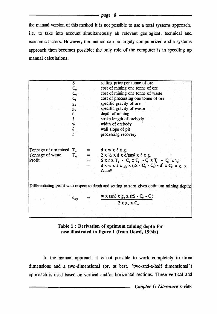
Table 1 Derivation of optimum mining depth for case in figure 1 8
Table 2 Discounted cash flows for alternative mining sequences in
figures 14-1 7
Chapter Three :
Table 1 Discounted cash flows from two mining sequences
Table 2 Step 1 in the simplex algorithm
Table 3 Step 5 in the simplex algorithm
Table 4
Table 5
Chapter Six :
Table 1
Table 2
Table 3
Table 4
Table 5
Table 6
Table 7
Step 5 iteration 2 in the simplex algorithm
Step 5 iteration 3 in the simplex algorithm
Pit plan evaluation
Order of priority of blocks
Mixed prioritization of blocks
Blocks produced in the first production period
Blocks produced in the second production period
Blocks produced in the third production period
Discounted alternatives in each production period
38
88
100
102
103
103
144
151
153
159
165
167
170
Contents

CHAPTER ONE
Optimal open pit design and optimal production scheduling: Literature review and survey of previous work
1. Optimal open pit design 2
1.1 Introduction 2
1.2 Optimization criteria 5
1.3 Review of methods for open pit optimization 6
1.3.1 Traditional pit design 7
1.3.2 Lerchs-Grossmann algorithm 9
1.3.2.1 Graph theory 9
1.3.2.2 Maximum flow techniques 11
1.3.3 Moving cones 12
1.3.4 Dynamic programming algorithm 14
1.3.5 The Korobov algorithm 16
1.3.6 Corrected form of the Korobov algorithm 24
1.3.7 The parameterization technique 29
2. Production schedule optimization 30
2.1 Introduction 30
2.2 Review of previous techniques for the optimization of
production schedules 32
2.2.1 Simulation 32
2.2.2 Linear programming 32
2.2.3 Integer programming 33
2.2.4 Dynamic programming 33
2.2.5 Graph and network theory 40
2.2.6 Heuristic methods 41
3. The objectives of the research programme 41
Chapter 1: Literature review

------------ page 2
1. Optimal open pit design
1.1 Introduction
An open pit mine is characterised physically by a large hole in the ground. The
determination of the shape and location of this hole with respect to the mineralization
are the essential features of the optimality problem. Once the optimal shape and
location of the pit are determined the mine must be equipped with the necessary
operating plant and labour. This development requires the investment of a large
amount of capital which must be repaid as quickly as possible. Many studies (eg,
Dowd, 1976, Lane, 1964) have shown that the combination of the time value of
money and the need to pay back the initial investment as quickly as possible require
operations to begin with a relatively high cut-off grade which then declines over the
life of the mine. Estimation of block grades and consequent cut-off grades is thus
essential for optimal mine planning. These estimations are based on the available
information gathered during the exploration and feasibility stages by a drilling and
sampling programme. From this information a model of the orebody is constructed
in the form of estimated block grades which are then used as the basis on which the
optimum open pit is designed and the optimal production schedule for mine design
is determined.
The objective of any optimal open pit design algorithm is to determine the
final pit limits of an orebody and its associated grade and tonnage, which will
maximize some specified economic and! or technical criteria whilst satisfying
practical operational requirements. Since the advent and widespread use of
computers, open pit design has been implemented by the application of different
methods and various algorithms, all with a common objective:
to maximize the overall mining profit within the designed pit limit
Chapter 1: Literature review

------------ page 3
One of the most important economic aspects of open pit mining is the cut-off
grade. There are many different types of cut-off grade each defined and used for a
different purpose. In the most general sense a cut-off grade is any grade:
or
• that is used for distinguishing between two different courses of action (e.g. to
mine or not to mine; to process or not to process; to separate marginal ore
from run-of-mine ore)
• that is used to classify material (e.g. into ore and waste; into graded fractions)
For the purposes of this work the term cut-off grade is used in its general
economic sense to distinguish between ore and waste. The cut-off grade is a very
important factor in mine planning as it affects the overall reserves of ore and the
amount of waste and overburden to be removed.
Cut-off grades are known as technico-economic parameters and are a complex
function of grade distributions and variables such as mining costs, processing costs
and metal prices. They define what is mined and what is milled from a mine's
output. To be optimal a cut-off grade must be such that it maximizes the realisable
total net discounted value of the orebody. If the cut-off grade is too high it will
reduce the mineral recovered and possibly the life of the mine; if it is too low the
cut-off will reduce the average grade (and hence profit) below acceptable levels.
It is important to differentiate between planning and the operational cut-off
grades. There are a number of techniques available for optimising cut-off grades.
Roman (1973) introduced dynamic programming as a means of optimising
production rates and Dowd (1976) extended this work to include cut-off grades.
Lane (1964) is generally regarded to have provided landmarks in the understanding
and general communication of cut-off grade theory and its application. He introduced
(Lane, 1964) three stages in determining the optimal cut-off grade: extraction,
processing and marketing. Costs were determined for each stage as well as the effect
Chapter 1: Literature review

-------------------------page 4 --------------------------
on the Present Value of each stage of varying cut-off grade. Blackwell (1970)
revised Lane's method, again with three stages as the pit, the concentrator and the
market constraints. With the inclusion of an additional time cost to be borne by the
operation, he was able, by the use of a computer-based algorithm, to determine the
maximum Net Present Value, which resulted again in a declining cut-off grade.
Perhaps one of the best definitions of cut-off grade is that of Taylor (1972).
Taylor fIrstly defmes the breakeven grade as that grade from which the recoverable
revenue exactly balances the costs of mining, treatment and marketing, and the cut
off grade is any grade that, for any specifically reason is used to separate two
courses, e.g. to mine or to leave, to mill or to dump according to their appropriate
conditions. Such a definition allows the forecasting of future marketing conditions
in terms of probability.
The essential difference between planning and operational cut-off grades is
the time scale to which they relate. Planning cut-off grades are long term and
generally required before production starts to define geographically and
quantitatively the potential ore limits. Operating cut-off grades are those required
during production to defIne on a shorter term basis those parcels of ore that may
contribute to unmined ore reserves or to streams of broken ore.
The use of a planning cut-off grade constructed on breakeven principles
certainly appears justifIable for the determination of pit limits, whereas the operating
cut-off grade appears justifIed for production scheduling. In the first specification it
is assumed that when a cut-off grade is applied to the block then the whole block is
either above or below the cut-off grade, i.e. the selective mining unit is the whole
block. The second specification allows for selective mining on a scale smaller then
the planning block.
Almost all methods are based on orebody block models which are either a :
Chapter 1: Literature review

------------ page 5 -------------
or a
o Revenue block model obtained by dividing the deposit into blocks
and assigning a revenue value to each block according to its estimated
grade and tonnage above a specified cut-off grade
o Block grade model which is usually in the form of average grade
above a specified cut-off grade.
There are a number of other methods which are essentially based on
geological models and ignore the block concept but, in general, these are only
applicable in the simplest of orebodies such as those described in section 1.3.1 of
this Chapter. More general applications of geological models are not considered here
because the models are not suited to pit design.
Although many methods have been proposed over the past 30 years very few
enjoy any significant use today. The major reason for this is that most methods
cannot be guaranteed to yield a true optimum.
The initial section of this thesis examines the general understanding behind
the concept of optimal pit detennination followed by some of the techniques which
are applicable in mining operations.
1.2 Optimization criteria
The frrst step in any optimization problem is to define the optimization criteria. For
pit design there can be any number of criteria: technical, geological, economic or
a combination of all three. The most commonly used criteria are economic such as
maximum profit, maximum extraction of metal, maximum net present value, optimal
mine life. Of these, the most widely accepted are variants of maximum profit.
However, an orebody can be mined at a range of cut-off grades each of which (at
least over practical values) will yield similar amounts of metal for different tonnages
Chapter 1: Literature review

-------------------------page 6 --------------------------
of ore mined. Because of the time value of money it will always be more profitable
to mine at a higher cut-off grade in the early years and then at a declining cut-off
grade over the later years. Thus the optimizing criterion should be maximum net
present value rather than maximum total profit. There are, however, very difficult
problems with implementing net present value as an optimizing criterion which will
be discussed in Chapter 2.
For manual methods of pit design it is generally very difficult, if not
impossible, to use criteria such as maximum net present value or even maximum
total profit as an optimizing criterion. The implicit optimizing criterion in most
manual methods is, for a given cut-off grade, either maximum extraction of metal
or minimum extraction of waste.
Whatever the method the optimizing criteria may be overridden by other
considerations such as technical constraints (e.g., safe pit slopes), environmental and
planning requirements or government policies, the latter often imposed in the form
of taxation schemes. Although these factors are important they are not explicitly
considered in the remainder of this thesis. The purpose here is to examine and derive
methods that optimize economic criteria. However, many technical constraints (such
as pit slopes) will be included inherently in the methods or the formulation of the
models.
1.3 Review of methods for open pit optimization
In this review of the literature attention is restricted to those optimization techniques
in common use. In particular, attention is focused on those techniques used
frequently in commercial and research software for the determination of the optimum
open pit limits; these methods include the Lerchs-Grossmann algorithm, the various
moving cone algorithms, dynamic programming, the corrected form of the Korobov
Chapter 1: Literature review

------------------------page 7 -------------------------
algorithm and the parameterization technique. In addition, traditional pit design, in
its original form and in its later, computerised form will be discussed.
1.3.1 Traditional pit design
For simple, well-defined mineralizations there is often no need to use sophisticated
computer algorithms to design optimal pits: the true optimum can be found by the
application of well-known, elementary mathematical techniques. An example of such
simple cases (taken from Dowd, 1994a) is in the mining of dipping, stratigraphically
defined structures of uniform grade as shown in figure 1. As the pit is deepened
more and more waste must be removed. Here the pit shape can be defined as a
function of the net value of mining ore and waste down to a given depth. Once the
pit slopes are defined the objective is to determine the depth which gives the
maximum profit. Simple calculus can be used to determine the optimal depth and
thus optimal pit shape. To illustrate this consider the simple case shown in figure 1.
Assume that the ore has
constant width wand a strike
length of f. Table 1 shows the
derivation of the optimal
mining depth. Similar, but
more complex, formulas can
be derived for more
" " " " " " " " e " /
Figure 1
/
/ /
/
/ /
/ /
/
d
realistically shaped and oriented stratigraphic deposits or sequences.
In the more general case, where the grades vary in three dimensions and the
ore is not confined to simple stratigraphic boundaries, such exact elementary
approaches are not possible and a more complex algorithmic solution is required. A
few years ago, even in cases such as this, the determination of optimum pit limits
was done by hand using traditional, logical pit design methods based largely on
cross-sectional interpretations of the mineralization and on grade contour maps. In
Chapter 1: Literature review
------------ page 8
the manual version of this method it is not possible to use a total systems approach,
Le. to take into account simultaneously all relevant geological, technical and
economic factors. However, the method can be largely computerized and a systems
approach then becomes possible; the only role of the computer is in speeding up
manual calculations.
Tonnage of ore mined To Tonnage of waste T w
Profit
= = = =
selling price per tonne of ore cost of mining one tonne of ore cost of mining one tonne of waste cost of processing one tonne of ore specific gravity of ore specific gravity of waste depth of mining strike length of orebody width of orebody wall slope of pit processing recovery
dxwxtxg, 2 x Ih x d x d/tan8 x t x & S x r x To - Co x To - G x 1;, - G.. x 't d x w x t x go x (rS .. G, - G) - d2
X ~ x &. x l/tan8
Differentiating profit with respect to depth and setting to zero gives optimum mining depth:
dept = w x tan8 x go x (rS - G, - G) 2 x gw x Cw
Table 1 : Derivation of optimum mining depth for case illustrated in figure 1 (from Dowd, 1994a)
In the manual approach it is not possible to work completely in three
dimensions and a two-dimensional (or, at best, "two-and-a-half dimensional It)
approach is used based on vertical and/or horizontal sections. These vertical and
Chapter 1: Literature review

------------------------page 9 --------------------------
horizontal sections (or, in fact, sections of any orientation) are only approximations
to the three-dimensional shape of the pit; the pit shape on any section is designed
independently of the shape on the other sections and the results are then modified
to create a continuous (smoothed) pit surface.
This "two-and-a-half dimensional" approach was also applied in the early
computerised attempts at optimal open pit design. The best example of this is
Johnson's dynamic programming algorithm (Johnson, 1971), which is described in
section 1.3.4. Whilst it is easy to find examples for which such an approach fails to
fmd the optimal solution it was, nevertheless, a useful, approximate technique at a
time when computers were very much slower and less powerful than they are today.
1.3.2 Lerchs-Grossmann algorithm
The fITst rigorously optimal method for the general case was proposed by Lerchs and
Grossmann (1965). This method overcomes the limitations of traditional pit design
and can be proved always to yield the optimal solution. The Lerchs-Grossmann
algorithm is based on Graph Theory.
1.3.2.1 Graph theory
The graph theory approach developed by Lerchs and Grossmann (1965), for the
determination of the optimum pit limit is based on the construction of a maximum
closure of a graph. The l..erchs-Grossmann algorithm converts the three-dimensional
grid of blocks in the orebody model into a directed graph. Each block in the grid is
represented by a vertex which is assigned a mass equal to the net revenue value of
the corresponding block. The vertices are connected by arcs in such a way that the
connections leading from a particular vertex to the surface define the set of vertices
(blocks) which must be removed if that vertex (block) is to be mined. A simple two
dimensional example is shown in figure 2.
Chapter 1: Literature review

------------page 10 ------------
Figure 2 : Directed graph representing a 2-D deposit model
nodes represent blocks and arcs define mining constraints
Vertices connected by an arc pointing away from a vertex are termed
successors of that vertex, i.e. the vertex y is a successor of the vertex x if there
exists an arc directed from x to y. The set of all successors of x is denoted rx. For
example, in figure 2, rX9 = {X2' X3 , ~ }. A closure of a directed graph, which
consists of a set of vertices X, is a set of vertices Y C X such that if x E Y then
rx E Y. For example, in figure 2, Y = {x l' X 2' X3' X4 , Xs , Xs , X9 , "0 } is a
closure of the directed graph. The value of a closure is the sum of the masses
(revenue values) of the vertices in the closure. Each closure defines a possible pit;
the closure with the maximum value defines the optimal pit.
This method is the only method which can be proved rigorously,
mathematically always to lead to the correct optimal solution. However, a number
of recently published new methods have also made similar claims but they remain
to be independently verified.
Most of the stated disadvantages of the Lerchs-Grossmann are perceived
rather than real. The most commonly stated disadvantages are:
• Complexity of the method
• Computing time
• Difficulty of incorporating variable pit slopes
Chapter 1: Literature review
------------page 11 -------------
Complexity
In principle, it is desirable that users of a technique understand the mechanisms
being used otherwise it becomes a "black box" which may generate results that
cannot be properly assessed and questioned. However, it might also be said that once
a technique has been proved and implemented in a validated software package it is
no longer necessary for the user to have a detailed knowledge of the workings of the
algorithm. After all, no user of a proprietary CAD package demands to understand
the algorithms that it employs before he or she agrees to use it. Thus complexity of
the algorithm cannot really be accepted as a disadvantage. The important things are
for the user to be aware of any limitations in the algorithm and! or in the software
implementation.
Computing time
There is no doubt that the Lerchs-Grossmann algorithm requires significantly more
computing time than most of its (non-optimal) competitors. Increased computing
time is the price to be paid for a truly optimal solution. However, computing speed
is rapidly being increased and a PC can now solve optimal open pit problems that
only a few years ago could only be attempted on large mainframes. Computing tim~
is fast becoming irrelevant.
Variable pit slopes
This has been a problem in the past because of the difficulty of defining the joining
arcs in the network (see figure 2) in any general and flexible sense. However, there
are now a number of published solutions to this problem; see, for example, Dowd
and Onur (1993).
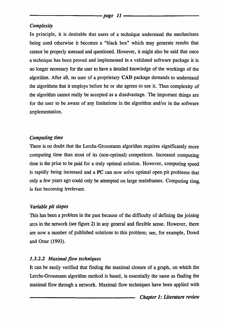
1.3.2.2 Maximal flow techniques
It can be easily verified that finding the maximal closure of a graph, on which the
Lerchs-Grossmann algorithm method is based, is essentially the same as finding the
maximal flow through a network. Maximal flow techniques have been applied with
Chapter 1: Literature review
------------page 12 ------------
some success, but they do not seem to have been adopted to any great extent largely
because they share the same perceived disadvantages as the Lerchs-Grossmann
method.
Of the various known alternative algorithms which have been employed to
overcome the perceived disadvantages and limitations of the Lerchs-Grossmann
algorithm the most well-known are the moving cone algorithm, dynamic
programming, the corrected form of the Korobov algorithm and the parameterization
technique.
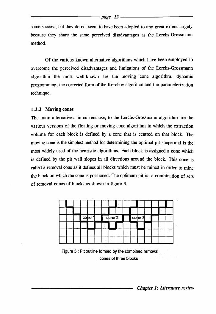
1.3.3 Moving cones
The main alternatives, in current use, to the Lerchs-Grossmann algorithm are the
various versions of the floating or moving cone algorithm in which the extraction
volume for each block is defined by a cone that is centred on that block. The
moving cone is the simplest method for determining the optimal pit shape and is the
most widely used of the heuristic algorithms. Each block is assigned a cone which
is defined by the pit wall slopes in all directions around the block. This cone is
called a removal cone as it dermes all blocks which must be mined in order to mine
the block on which the cone is positioned. The optimum pit is a combination of sets
of removal cones of blocks as shown in figure 3.
I .... ~e 1 - :>ne2
roo--1e ~ J co c co
Figure 3 : Pit outline formed by the combined removal
cones of three blocks
I
Chapter 1: Literature review
------------page 13 ------------
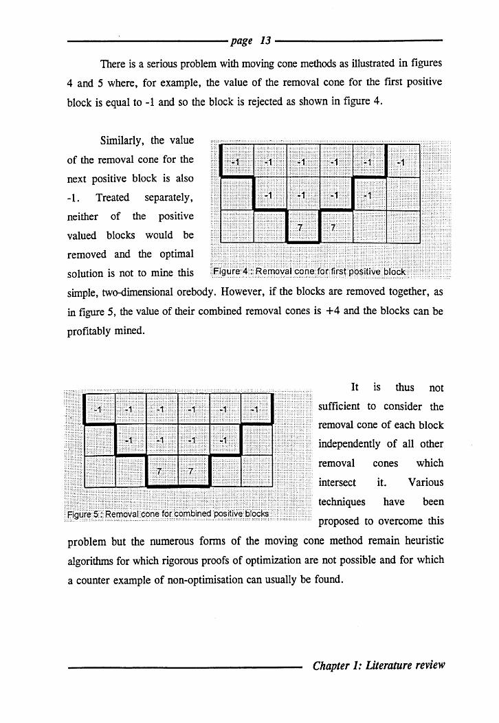
There is a serious problem with moving cone methods as illustrated in figures
4 and 5 where, for example, the value of the removal cone for the first positive
block is equal to -1 and so the block is rejected as shown in figure 4.
Similarly, the value
of the removal cone for the
next positive block is also
-1. Treated separately,
neither of the positive
valued blocks would be
removed and the optimal
solution is not to mine this
,:-: ::-:
l:::::: 1:::,:-: lot:
'!'OJ
:,;, ... .:: ::-:
::
:T1 ::. -::::. .. ....•... :.:.:: ........ . /-:::' ::,::: :::::
:::. ::-::::::
::: ...
::::,
simple, two-dimensional orebody. However, if the blocks are removed together, as
in figure 5, the value of their combined removal cones is +4 and the blocks can be
profitably mined.
.... ::: It is thus not ::
:::! i:' ::::::
"-"'1: .::2- :,: I:>: :~~\: :::
sufficient to consider the : :::
} :::
::: ::::; "j.: :;:::. :;; :.:':,:.; ::::::::::>:
:;1. ::::
:F:: :\./:::: :.:;
;: removal cone of each block
independently of all other ::::: :::: ·n :en ::
:: 1:':::1::-:: ::::.: :::
.: removal cones which .::: c:'::::.:.:.: :::::: .. ';' ::::: intersect it. Various
techniques have been ... ::i!-:f :en:','" ·i.J111 ;1,. fJ t)ll 'e blocks':
:;::-: ::: proposed to overcome this
problem but the numerous forms of the moving cone method remain heuristic
algorithms for which rigorous proofs of optimization are not possible and for which
a counter example of non-optimisation can usually be found.
Chapter 1: Literature review

------------page 14 -------------
1.3.4 Dynamic programming algorithm
Dynamic programming was advanced as an early alternative to the Lerchs
Grossmann algorithm.
Dynamic programming is the name given to a technique used to find optimal
sequences of decisions for problems which can be described as sequential decision
processes. Problems to which the technique can be applied must be such that they
can be divided into a sequence of smaller problems for each of which an optimal
solution can be found. Problems which can be solved by dynamic programming are
characterized by :
@a system
@stages
@state
@optimal policy
etransfer function
erecursive relationship
which defines the problem to be optimized.
which are sub-problems into which the overall problem
can be divided; they usually correspond to periods of
time.
the condition of the system at any given stage.
sequence of decisions which optimizes a criterion
function.
an expression which defines the manner in which the
state of the system at one stage is related to the state
of the system at the preceding stage, ie the manner in
which the next state will be determined by the current
state and decision.
is a mathematical expression which defines the optimal
solution at each stage.
Chapter 1: Literature review
------------page 15 ------------
Dynamic programming is based on the application of a simple property of
multi-stage decision processes. This property has been formulated by Bellman (1957)
in his principle of optimality as:
An optimal policy has the property that whatever the initial state and initial
decision are, the remaining decisions must constitute an optimal policy with
regard to the state resulting from the first decision.
In other words, an optimal set of decisions has the property that if a
particular decision is optimal, all subsequent decisions that depend on that decision
must also be optimal.
Unlike techniques such as linear programming there is no standard
mathematical formulation of dynamic programming and so particular equations
(transfer functions and recursive relationships) must be developed to fit each
individual situation. As a theory, dynamic programming was first formulated by
Bellman (1957). It has been applied successfully to a number of mining problems
(David and Dowd, 1976, Dowd, 1976, Dowd, 1980, Dowd and Elvan, 1987, Onur
and Dowd, 1993).
The dynamic programming formulation of the optimal open pit problem is
relatively simple. The decisions are all of the possible combinations of blocks which
satisfy the mining constraints and the problem is to choose the sequence of decisions
which maximises the net present value. This is a particularly attractive approach as
it will solve the problem on the basis of the ideal criterion. In principle, dynamic
programming will yield the correct optimal solution. However, in practice, the large
numbers of blocks (and hence combinations of decisions) in orebody block models
result in too many alternative decisions and, as a consequence, computing time and
storage are prohibitive, even allowing for recent advances in PC technology.
Chapter 1: Literature review

------------page 16 ------------
In an attempt to overcome these problems the method has been implemented
by subdividing the orebody block model into a sequence of two-dimensional vertical
slices of blocks and applying dynamic programming to these two-dimensional arrays
(Johnson, 1971). This leads to a series of correct solutions for each of the two
dimensional slices, i.e. considering each slice as a separate, independent "orebody".
The sequence of two-dimensional optima are then combined, by another dynamic
programming technique, into a quasi-optimal solution for the total three-dimensional
block model. This approach may yield a solution which is not significantly different
to the true optimum. However, there is no way of knowing how close any solution
is to the true optimum and, in practice, the difference may be highly significant. It
is very easy to devise simple examples for which the two-dimensional, approximate
dynamic programming method will yield solutions significantly different to the true
optimum.
Notwithstanding the time and storage problems associated with the full
implementation of the dynamic programming method it still attracts interest as a
possible method for optimal open pit design. To be practical and efficient an
accurate method must be found to eliminate all sub-optimal decision sequences as
soon as they arise. Such an approach would be a fruitful avenue for future research.
1.3.5 The Korobov algorithm
This method is originally due to Korobov (1974) and is reported in David, Dowd
and Korobov (1974), Dowd and Onur (1993). It is a cone based algorithm which
uses the idea of allocating values from positive blocks against the negative or zero
blocks contained in the extraction cones of the positive blocks. A flowchart for the
algorithm is given in Korobov (1974).
An extraction cone is assigned to every positive block in the orebody model
and the positive block values within each cone are allocated against the negative
block values within the cone until no negative block remains or until the values of
Chapter 1: Literature review
------------page 17 ------------
the positive block have all been allocated. If, when this allocation is completed, the
positive block on which the extraction cone is based remains positive, then this
extraction cone is accepted as a member of the optimum solution set. When a non
empty extraction cone is added to the solution set, the algorithm starts again from
the beginning with original block values restored to the blocks not yet extracted from
the block model. If an extraction cone is empty the positive block is added to the
solution and the algorithm proceeds on the current or next level.
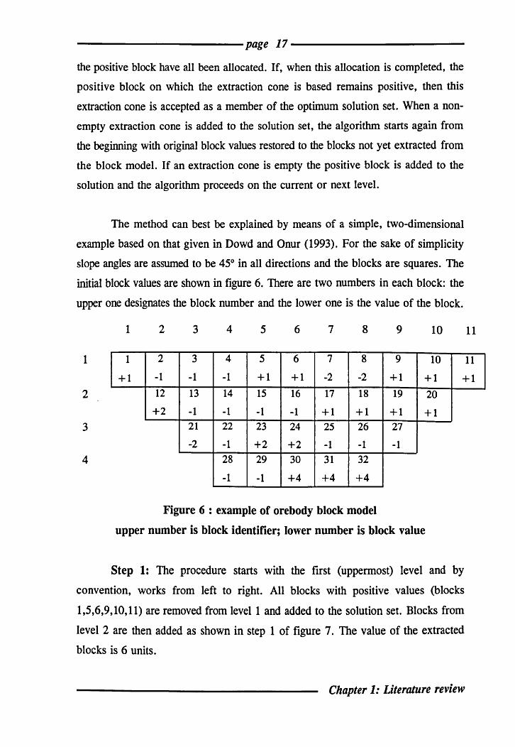
The method can best be explained by means of a simple, two-dimensional
example based on that given in Dowd and Onur (1993). For the sake of simplicity
slope angles are assumed to be 45° in all directions and the blocks are squares. The
initial block values are shown in figure 6. There are two numbers in each block: the
upper one designates the block number and the lower one is the value of the block.
1 2 3 4 5 6 7 8 9 10
1 1 2 3 4 5 6 7 8 9 10
11
11
+1 -1 -1 -1 +1 +1 -2 -2 +1 +1 +1 2 12 13 14 15 16 17 18 19 20
+2 -1 -1 -1 -1 +1 +1 +1 +1 3 21 22 23 24 25 26 27
-2 -1 +2 +2 -1 -1 -1 4 28 29 30 31 32
-1 -1 +4 +4 +4
Figure 6 : example of orebody block model
upper number is block identifier; lower number is block value
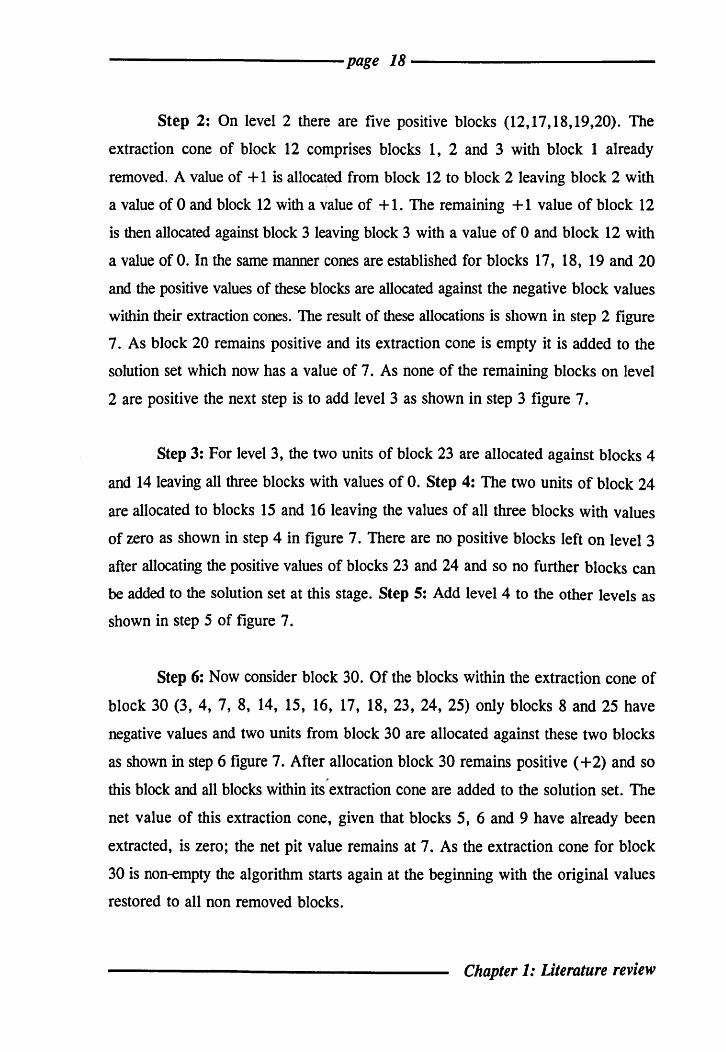
Step 1: The procedure starts with the first (uppermost) level and by
convention, works from left to right. All blocks with positive values (blocks
1,5,6,9,10,11) are removed from level 1 and added to the solution set. Blocks from
level 2 are then added as shown in step 1 of figure 7. The value of the extracted
blocks is 6 units.
Chapter 1: Literature review
----------------------page 18-----------------------
Step 2: On level 2 there are five positive blocks (12,17,18,19,20). The
extraction cone of block 12 comprises blocks 1, 2 and 3 with block 1 already
removed. A value of + 1 is allocated from block 12 to block 2 leaving block 2 with
a value of 0 and block 12 with a value of + 1. The remaining + 1 value of block 12
is then allocated against block 3 leaving block 3 with a value of 0 and block 12 with
a value of O. In the same manner cones are established for blocks 17, 18, 19 and 20
and the positive values of these blocks are allocated against the negative block values
within their extraction cones. The result of these allocations is shown in step 2 figure
7. As block 20 remains positive and its extraction cone is empty it is added to the
solution set which now has a value of 7. As none of the remaining blocks on level
2 are positive the next step is to add level 3 as shown in step 3 figure 7.
Step 3: For level 3, the two units of block 23 are allocated against blocks 4
and 14 leaving all three blocks with values of O. Step 4: The two units of block 24
are allocated to blocks 15 and 16 leaving the values of all three blocks with values
of zero as shown in step 4 in figure 7. There are no positive blocks left on level 3
after allocating the positive values of blocks 23 and 24 and so no further blocks can
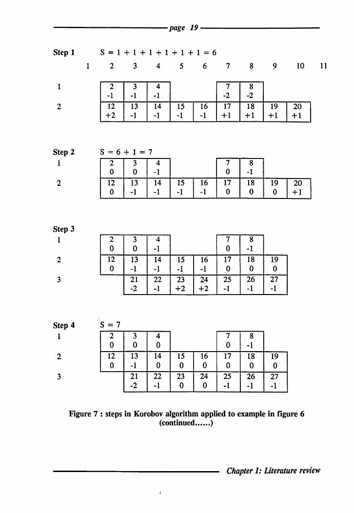
be added to the solution set at this stage. Step 5: Add level 4 to the other levels as
shown in step 5 of figure 7.
Step 6: Now consider block 30. Of the blocks within the extraction cone of
block 30 (3, 4, 7, 8, 14, 15, 16, 17, 18, 23, 24, 25) only blocks 8 and 25 have
negative values and two units from block 30 are allocated against these two blocks
as shown in step 6 figure 7. After allocation block 30 remains positive (+ 2) and so
this block and all blocks within its extraction cone are added to the solution set. The
net value of this extraction cone, given that blocks 5, 6 and 9 have already been
extracted, is zero; the net pit value remains at 7. As the extraction cone for block
30 is non-empty the algorithm starts again at the beginning with the original values
restored to all non removed blocks.
Chapter 1: Literature review
---------------------page 19----------------------Step 1 S = 1 + 1 + 1 + 1 + 1 + 1 = 6
1 2 3
1 2 3 -1 -1
2 12 13 +2 -1
Step 2 S = 6 + 1 = 7 1
2
Step 3 1
2
3
2 0
12 0
2 0
12 0
Step 4 S = 7 1 2
0
2 12 0
3
3 0
13 -1
3 0
13 -1 21 -2
3 0
13 -1 21 -2
4 5 6
4 -1 14 15 16 -1 -1 -1
4 -1 14 15 16 -1 -1 -1
4 -1 14 15 16 -1 -1 -1 22 23 24 -1 +2 +2
4 0
14 15 16 0 0 0
22 23 24 -1 0 0
7 8 9 10
7 8 -2 -2 17 18 19 20 +1 +1 +1 +1
7 8 0 -1
17 18 19 20 0 0 0 +1
7 8 0 -1
17 18 19 0 0 0
25 26 27 -1 -1 -1
7 8 0 -1
17 18 19 0 0 0
25 26 27 -1 -1 -1
Figure 7 : steps in Korobov algorithm applied to example in figure 6 (continued •••••• )
Chapter 1: Literature review
11
--------------------page 20---------------------Step 5
1
2
3
4
2 0
12 0
3 0
13 -1 21 -2
4 0
14 0
22 -1 28 -1
Step 6 S = 7 + (0) = 7 1
2
3
4
Step 7
1
2
Step 8 1
2
2 3 4 0 0 0
12 13 14 0 -1 0
21 22 -2 -1
28 -1
S=7+1=8 2
-1 12 13
+2 -1
S=8+1=9 2 0
12 13 +1 -1
7 0
15 16 17 0 0 0
23 24 25 0 0 -1
29 30 31 -1 +4 +4
7 0
15 16 17 0 0 0
23 24 25 0 0 0
29 30 31 -1 +2 +4
8 -1 18 0
26 -1 32 +4
8 0
18 0
26 -1 32 +4
19 0
27 -1
19 0
27 -1
fl9l ~
Figure 7 ( •••••••• continued •••••••• )
Chapter 1: Literature review

----------------------page 21-----------------------
Step 9 S = 9
2 13 -1
3 21 22 -2 -1
4 28 -1
Step 10 S = 9 + 3 + 3 = 15
2
3
4
Step 11
1
2
3
4
13 -1 21 22 -2 -1
28 -1
13 -1 21 22 -2 -1
28 -1
26 27 -1 -1
29 31 32 -1 +4 +4
26 27 0 0
29 31 32 -1 +3 +3
29 -1
S = 15
Figure 7 ( ••••• continued)
Add level 1; there are no positive blocks and thus none can be removed. Step
7: Add level 2 as shown in step 7 in figure 7. The extraction cone of block 19 is
empty and this block is added to the solution giving a net pit value of 8. Step 8:
Block 2 is the only block within the extraction cone of positive block 12 and one
Chapter 1: Literature review
------------page 22 -------------
unit from the latter is allocated against the former. Block 12 and its extraction cone
are removed giving a net pit value of 9 as shown in step 8 in figure 7.
Step 9: Add level 4 as shown in step 9 in figure 7. Step 10: Block 26 is
allocated one unit from block 31 and block 27 is allocated one unit from block 32
as shown in step 10 in figure 7. Step 11: As blocks 31 and 32 remain positive after
allocation they and the blocks in their extraction cones are added to the solution set
giving the final pit shape shown in step 11 of figure 7. The net pit value is 15 and
the only unmined blocks remaining in the block model are 13, 21, 22, 28 and 29.
Soon after the method had been introduced it was realised that the algorithm
did not reach the optimum solution in all cases. For some types of block models the
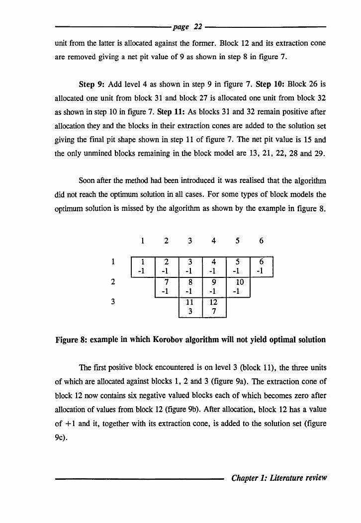
optimum solution is missed by the algorithm as shown by the example in figure 8.
1 2 3 4 5 6
1 1 2 3 4 5 6 -1 -1 -1 -1 -1 -1
2 7 8 9 10 -1 -1 -1 -1
3 11 12 3 7
Figure 8: example in which Korobov algorithm will not yield optimal solution
The frrst positive block encountered is on level 3 (block 11), the three units
of which are allocated against blocks 1, 2 and 3 (figure 9a). The extraction cone of
block 12 now contains six negative valued blocks each of which becomes zero after
allocation of values from block 12 (figure 9b). After allocation, block 12 has a value
of + 1 and it, together with its extraction cone, is added to the solution set (figure
9c).
Chapter 1: Literature review

------------page 23 ------------
1 2 3 4 5 6 1 2 3 4 5
1 1 2 3 4 5 6 1 2 3 4 5 0 0 0 -1 -1 -1 0 0 0 0 0
2 7 8 9 10 7 8 9 10 -1 -1 -1 -1 -1 0 0 0
3 11 12 11 12 0 +7 0 +1
(a) (b)
1 1 0
2 7 0
3 11 +1
(c)
Figure 9 : steps in the Korobov algorithm applied to the example in figure 8
The extraction cone of block 12 has a value of -1 which is the net pit value
at this stage. The algorithm now starts again from the beginning with the original
values restored to the non-removed blocks. There are two negative valued blocks (1
and 7) in the extraction cone for block 11 and after allocation (figure 9c) block 11
remains positive. Block 11 and the blocks within its extraction cone, with a net value
of + 1, are added to the solution set. The solution yielded by the algorithm is thus
to mine all blocks at a net profit of zero.
The error is caused by blocks which are common to both extraction cones.
Blocks 2, 3, 4, 5, 8 and 9 are common blocks. Blocks 1 and 7 are only members
of extraction cone 1 and are not in common with extraction cone 2. If the allocation
procedure began with these non-common blocks the error would not occur. Thus if
Chapter 1: Literature review
6
6 0

------------page 24 -------------
two or more cones have blocks in common, allocation must first be made against the
non-common blocks; allocation against common blocks is done only after the values
of all non-common negative blocks have been reduced to zero.
1.3.6 Corrected form of the Korobov algorithm
The fault in the Korobov algorithm was rectified by Dowd and Onur (1993). The
correction to the Korobov algorithm is based on the following logic:
If two or more cones have blocks in common, then blocks not in common
must be paid for first; common blocks are only paid for after all blocks not
in common have been paid for.
The number of cone searches is significantly reduced by means of paths
which define links between zero valued blocks in an extraction cone and any
negative block in an intersecting cone. A flowchart for the algorithm is given in
Dowd and Onur (1993). The corrected form of the Korobov algorithm can be
demonstrated by means of the simple, 3-D example taken from Dowd and Onur and
shown in figure 10.
Suppose that there are two levels and the slope angle is 45°. The block
dimensions are the same for all directions. In this example, extraction cones for
blocks on level 2 are dermed by taking the 9 blocks on level lover a positive block
on level 2. The extraction cone for positive block (i,j,2) on level 2 consists of
blocks (m, n, 1) where m=i-l,i+l and n=j-l,j+1.
As there is no positive block on level 1 the search moves to level 2 and starts
from block (2,2,2) (as this is the first cone of the model it will be called cone 1).
The member blocks for cone 1 are blocks (m, n, 1) where m= 1,3 and n= 1,3. The
original allocation is shown in figure 11 in which each block has two numbers. The
upper number designates the cone from which this block has been allocated a value;
the lower number is the net block value after allocation.
Chapter 1: Literature review
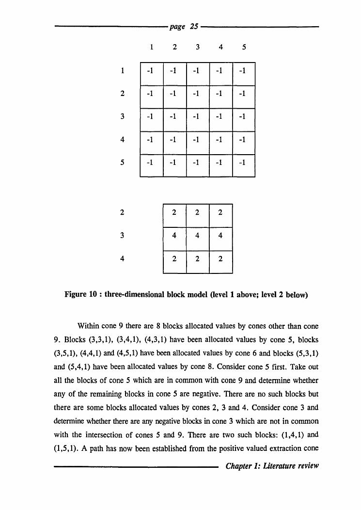
------------page 25 ------------
1 2 3 4 5
1 -1 -1 -1 -1 -1
2 -1 -1 -1 -1 -1
3 -1 -1 -1 -1 -1
4 -1 -1 -1 -1 -1
5 -1 -1 -1 -1 -1
2 2 2 2
3 4 4 4
4 2 2 2
Figure 10 : three-dimensional block model (level 1 above; level 2 below)
Within cone 9 there are 8 blocks allocated values by cones other than cone
9. Blocks (3,3,1), (3,4,1), (4,3,1) have been allocated values by cone 5, blocks
(3,5,1), (4,4,1) and (4,5,1) have been allocated values by cone 6 and blocks (5,3,1)
and (5,4,1) have been allocated values by cone 8. Consider cone 5 first. Take out
all the blocks of cone 5 which are in common with cone 9 and determine whether
any of the remaining blocks in cone 5 are negative. There are no such blocks but
there are some blocks allocated values by cones 2, 3 and 4. Consider cone 3 and
determine whether there are any negative blocks in cone 3 which are not in common
with the intersection of cones 5 and 9. There are two such blocks: (1,4,1) and
(1,5,1). A path has now been established from the positive valued extraction cone
Chapter 1: Literature review

------------page 26 ------------
9 via cones 5 and 3 to a negative block. The path, in terms of blocks is: (5,5,1),
(3,3,1), (2,3,1), (1,4,1). This path defines the re-allocation: the value (+1)
previously allocated to block (2,3,1) by cone 3, is re-allocated to block (1,4,1); the
value (+ 1) which was previously allocated to block (3,3, 1) by cone 5 is re-allocated
to block (2,3,1); block (3,3,1) is allocated a value of +1 from cone 9 (ie, block
(4,4,2». There are no positive values in the block model and the algorithm stops.
The final form of the result is shown in figure 12.
1 2 3 4 5
1 1 2 3 0 0 0 -1 -1
2 1 2 3 5 6 0 0 0 0 0
3 4 4 5 5 6 0 0 0 0 0
4 4 4 5 6 6 0 0 0 0 0
5 7 7 8 8 9 0 0 0 0 0
2 1 2 3 0 0 0
3 4 5 6 0 0 0
4 7 8 9 0 0 +1
Figure 11 : step 1 in the corrected Korobov algorithm applied to the example in figure 10
Chapter 1: Literature review

------------page 27 ------------
1 2 3 4 5
1 1 2 .; .;
0 0 0 0 -1
2 1 k .; ::> 6 0 0 0 0 0
3 4 4 , , ()
0 0 0 0 0
4 4 4 5 6 6 0 0 0 0 0
5 7 7 8 8 9 0 0 0 0 0
2 1 2 3 0 0 0
3 4 5 6 0 0 0
4 7 8 9 0 0 0
Figure 12 : step 2 in the corrected Korobov algorithm applied to the example in figure 10
Note that an alternative path to a negative block could have been defined via
cone 2 - (5,5,1), (3,3,1), (2,2,1), (4,4,1) .. When alternative paths are available it is
irrelevant which is chosen : the algorithm will always lead to the same solution.
The corrected Korobov algorithm has also been applied to the same example
in figure 8, where the original Korobov algorithm misses the optimum solution. The
basis of the extraction cones for the positive blocks (3,3) and (3,4) are in level 3. In
a similar way after allocation each block of the two-dimensional example is
represented by two numbers. The upper number designates the cone from which this
block has been allocated a value; the lower number is the net block value after
allocation.
Chapter 1: Literature review

------------page 28 ------------
Blocks (1,2), (1,3), (1,4), (1,5), (2,3) and (2,4) are common blocks for both
cones 1 and 2. Bocks (1,1) and (2,2) are only members of extraction cone 1 and are
not common to cone 2. The same is true for blocks (l,6) and (2,5) which are only
members of extraction cone 2 and are not common to cone 1.
The non-common blocks are paid fIrst, starting with the extraction cone 1, two
units are allocated for blocks (1,1) and (2,2) leaving block (3,3) with a value of +1.
Two units are allocated against blocks (1,6) and (2,5), leaving block (3,4) of the
extraction cone 2 with a value of +5. These allocations are shown in the following
figure(a).
1
2
3
1
10 1
2
-1
o 1
3 4 5 6
-1 -1 -1 o 21 -1 -1 0 2 +11 +ri
Figure(a)
The algorithm re-starts again by paying the common blocks of the two cones.
One unit is allocated against block (1,2) leaving block (3,3) with a value of zero.
Five units are allocated against blocks (1,3), (1,4), (1,5), (2,3) and (2,4), leaving
block (3,4) with a value of zero. After this allocation is completed, the positive
blocks on which the extraction cones 1 and 2 were based are zero as shown in the
following fIgure(b). The algorithm stops.
Chapter 1: Literature review
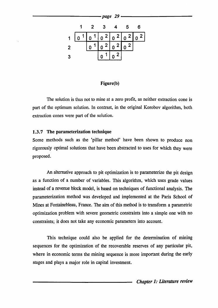
------------page 29 ------------
1
2
3
1
10 1
2
o 1
o 1
3 4 5 6
o 2 o 2 o 2 o 21
0 2 o 2 02
o 1 0 2
Figure(b)
The solution is thus not to mine at a zero profit, as neither extraction cone is
part of the optimum solution. In contrast, in the original Korobov algorithm, both
extraction cones were part of the solution.
1.3.7 The parameterization technique
Some methods such as the 'pillar method' have been shown to produce non
rigorously optimal solutions that have been abstracted to uses for which they were
proposed.
An alternative approach to pit optimization is to parameterize the pit design
as a function of a number of variables. This algorithm, which uses grade values
instead of a revenue block model, is based on techniques of functional analysis. The
parameterization method was developed and implemented at the Paris School of
Mines at Fontainebleau, France. The aim of this method is to transform a parametric
optimization problem with severe geometric constraints into a simple one with no
constraints; it does not take any economic parameters into account.
This technique could also be applied for the determination of mining
sequences for the optimization of the recoverable reserves of any particular pit,
where in economic terms the mining sequence is more important during the early
stages and plays a major role in capital investment.
Chapter 1: Literature review
------------page 30 ------------
The technique, described briefly above, is not rigorous, and has some
weaknesses on the economic side in comparison with other algorithms. It fonns the
fundamental basis behind Chapter 2 where it is discussed in detail.
2. Production schedule optimization
2.1 Introduction
Production scheduling is of vital importance in pit design and mine planning.
Production scheduling is the development of a sequence of depletion schedules
leading from the initial state of the deposit to the ultimate pit limits. Production
scheduling can be either long range or short range depending on the duration of the
scheduling period. Short range scheduling is the development of a depletion sequence
on a daily, weekly or monthly basis; long range scheduling is mainly concerned with
yearly plans and includes ore reserves, stripping ratios and capital investments.
The main objective of short and long range mine planning (scheduling) in an
open pit operation is to maximize the profits realized within every mining period and
throughout the life of the mine.
Although in practice production scheduling for both surface and underground
mining operations is similar in nature, a large range of techniques is applied in
solving such planning problems. The techniques consist of both rigid operational
research (OR) methods and practical procedures which are heuristically based.
It is widely expected that new and improved OR and mathematical techniques
will lead to better and more efficient methods of solving production scheduling
problems. The combination of these methods with the geostatistical simulation of
Chapter 1: Literature review

------------page 31 ------------
orebodies should lead to realistic scheduling packages which take adequate account
of uncertainties, errors in variables and risk.
In spite of their potential, very few OR techniques have been applied to the
solution of production scheduling problems in the mining industry and attention has
been focussed on the simplest of such techniques such as Linear Programming.
Although such techniques have been under-used this does not imply that they are not
applicable. Furthennore, the lack of use is attributed to a combination of many
causes, some of which are no longer relevant today.
Based on what has already been achieved, (operational research and computer
techniques) goal programming can be effectively applied to solve the problem of
open pit production planning optimization (Zhang, Cheng and Su (1993». Goal
programming is applied to overcome the limitations of single objective linear
programming applications.
A common approach to the solution of the problem of optimal open pit
production scheduling involves combining two or more operational research
techniques. In the work described in this thesis, Simulation and Linear Programming
have been combined to provide the basis of a method for the solution of the
problem.
The success of production scheduling methods will undoubtedly continue to
increase and spread to areas of mining where these methods have not yet been
applied. Success depends on the ability to fonnulate good operational research and
computer models.
Chapter 1: Literature review

------------page 32 -------------
2.2 Review of previous techniques for the optimization of
production schedules
The following sections give short resumes of some the operational research
techniques that are applicable to production scheduling problems in mining
operations.
2.2.1 Simulation
Simulation can be described as the use of a model to experiment with any given
system. It is one of the most powerful and versatile of the operational research
techniques available for assessing complicated, non-analytical problems. In
production scheduling problems, simulation is often used to help choose the correct
number of haulers assigned to an excavator, to evaluate different sizes of equipment,
or to assess the output of a given operating subsystem. However, it does not
guarantee the optimality of the solution and needs considerable computing time.
2.2.2 Linear programming
Linear programming is the most frequently applied operational research technique
in the solution of production scheduling problems in both surface and underground
mining. The most frequent applications have been in surface mining where the size
of the operation and the difficulty of meeting grade and resource constraints combine
to create a problem ideally suited to the technique. The Linear Program can be
solved by a general procedure known as the simplex method. A major restriction
still facing the implementation of the technique is the number of constraints which
must be kept relatively small. In some cases the complexity of multilevel open pit
mining, especially the precedence constraints, can lead to very large linear
programming models that can be computationally expensive, or in some cases
impossible, to solve.
Chapter 1: Literature review

------------page 33 ------------
2.2.3 Integer programming
In recent years, the use of integer programming methods has become more popular.
However, the applications of integer programming to production scheduling
problems seem to be oriented towards truck and shovel assignment problems. Integer
Programming is a less frequently used technique in optimal open pit scheduling
because of the complexity of the solution algorithms. A special group of integer
programming models is the 0-1 integer programming model, where each variable is
allowed to take a value of only 0 or 1. Such a model would be ideal for a production
scheduling problem since it permits the assignment of a 0-1 variable to each block
of the block model. For example a block can have a 0 value if it is not mined within
a mining period or a value of 1 if it is designated to be mined in that period.
However, the solution time of a 0-1 integer programming model tends to increase
exponentially with the number of variables. Although the solution algorithms
improve with time, there is little hope of even being able to solve really large
problems, such as the optimal open pit production scheduling problem.
2.2.4 Dynamic programming
Dynamic programming (D P) is another operational research technique that has been
used in solving open pit scheduling problems, e.g. Onur and Dowd (1993). It was
frrst applied to the open pit scheduling problem by Roman (1974). Wright (1989) has
also applied dynamic programming to the open pit scheduling problem.
The following formulation is taken from Onur and Dowd (1993). The system
is the orebody, the stages are mining periods and the state at any stage is the set of
blocks remaining in the ore body.
Let a be the ore/waste ratio,
b be the allowable limits of the grade,
c be the minimum operating room for equipment,
Chapter 1: Literature review

------------page 34 -------------
d be the working slope angle,
e be the maximum movement distance of the shovels,
r be the discount rate,
g be the production rate.
Further, let :
s
Itn(p,m(a,b,c,d,e,r,g»
be the total discounted profit after n decisions placing
the system in state p when an optimal decision policy
has been followed.
be the set of all possible decisions which satisfy all the
scheduling constraints.
be the immediate profit obtained by taking the decision
m, which is a function of a, b, c, d, e, r, g, and thus
placing the system in state p.
T(n-l,p,m(a,b,c,d,e,r,g» be the state of the system at step n-l as a result of
taking decision m(a,b,c,d,e,r,g) at step n. i.e. the
transfer function (noting that the method uses reverse
chronology).
The principle of optimality is then expressed in the following recursive relationship:
fip) =( ( b dmax ) E S){Rn(p,m(a,b,c,d,e,r,g)+tl (T(n,p,m(a,b,c,d,e,r,g»} m a, ,c, ,e,r,g
The dynamic programming formulation of the scheduling problem can best
be explained with a simple example taken from Onur and Dowd (1993). In this
example some assumptions have been made for the sake of simplicity but in a real
case all relevant characteristics of the mine and the orebody must be applied to the
formulation.
Chapter 1: Literature review

------------page 35 ------------
In this example the assumptions are :
1) the working slope angle is 45°
2) a total of three positive blocks (which represent ore) and between three and
five negative blocks (which represent waste) can be mined in the same stage
to represent a specific stripping ratio,
3) the discount rate is 10%,
4) minimum access space is one block,
5) there are no limitations on the number of shovels or on where they can work.
The orebody to be scheduled is shown in figure 13.
1 2 3 4 5 6 7 8 9
1 0.5 0.5 0.5 0.5 0.5 0.5 1.0 1.5 1.5 -1 -1 -1 -1 -1 -1 +2 +3 +3
2 1.0 1.0 1.0 0.5 0.5 0.5 0.5 +2 +2 +2 -1 -1 -1 -1
3 0.5 1.5 0.5 0.5 1.5 -1 +3 -1 -1 +3
4 1.5 2.0 2.5 +3 +4 +5
Figure 13 : orebody to be scheduled upper number is grade; lower number is revenue x lOZ
To keep the example simple, only the four possible schedules shown in
figures 14, 15, 16 and 17 will be considered here; table 2 displays the discounted
value of each decision in each stage.
Chapter 1: Literature review

----------------------page 36-----------------------
1 2 3 4 5 6 7 8 9
1 4 3 2 2 2 1 1 1 1
2 4 3 2 2 2 1 1
3 4 3 3 3 2
4 4 4 3
Figure 14 : solution no. 1 to scheduling problem in figure 13 number in block is the period in which block is mined
1 2 3 4 5 6 7 8 9
1 3 2 2 2 2 1 1 1 1
2 3 2 2 2 2 1 1
3 3 3 3 4 4
4 3 4 4
Figure 15 : solution no. 2 to scheduling problem in figure 13
Chapter 1: Literature review
LEEDS UNrVERSITV UBRARY

----------------------page 37-----------------------
1
2
3
4
1
1
2
1
1
3 4
1 1
1 1
2 2
3
5 6 7 8 9
1 2 2 3 3
2 2 3 4
3 4 4
4 4
Figure 16 : solution no. 3 to scheduling problem in figure 13
1
2
3
4
1 2 3 4 5 6 7 8 9
1 1 1 1 1 2 2 2 3
1 1 1 2 2 3 4
3 3 3 4 4
3 4 4
Figure 17 : solution no. 4 to scheduling problem in figure 13
Chapter 1: Literature review
------------page 38 ------------
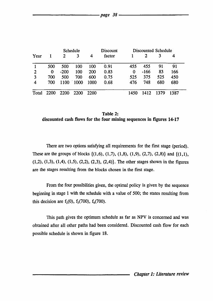
Schedule Discount Discounted Schedule Year 1 2 3 4 factor 1 2 3 4
1 500 500 100 100 0.91 455 455 91 91 2 0 -200 100 200 0.83 0 -166 83 166 3 700 500 700 600 0.75 525 375 525 450 4 700 1100 1000 1000 0.68 476 748 680 680
Total 2200 2200 2200 2200 1450 1412 1379 1387
Table 2: discounted cash flows for the four mining sequences in figures 14-17
There are two options satisfying all requirements for the first stage (period).
These are the groups of blocks {(1,6), (1,7), (1,8), (1,9), (2,7), (2,8)} and {(I,I),
(1,2), (1,3), (1,4), (1,5), (2,2), (2,3), (2,4)}. The other stages shown in the figures
are the stages resulting from the blocks chosen in the first stage.
From the four possibilities given, the optimal policy is given by the sequence
beginning in stage 1 with the schedule with a value of 500; the states resulting from
this decision are f2(0), f3(700), f4(700).
This path gives the optimum schedule as far as NPV is concerned and was
obtained after all other paths had been considered. Discounted cash flow for each
possible schedule is shown in figure 18.
Chapter 1: Literature review

-------------------------page 39--------------------------Cumulative dis<Xlunted ca.h floW'
1600 ~------------_
14001------------
12001--------·----
1000 ~-------.---.---
eoo~------
600 ~------~
.wo
200
o 1.00 2.00 3.00 4.00
Time period
_ S1 ~ S2 0 53 _ S4
Figure 18 : discounted cash flows for mining alternatives given in
figures 14-17
The tree representation of the example is as shown in figure 19.
0 I
I I 500 100
I I I I I I I I
a -200 100 200 I I I I I
700 500 700 600 I I I I I I I I
700 1100 1000 1000
Figure 19 : tree representation of npv of mining sequences from figures 14-17
Chapter 1: Literature review

-------------page 40 -------------
The main problem with the dynamic programming approach is the limitation
in terms of the total number of variables and constraints that can be taken into
account. Every dynamic programming model suffers from the 'dimensionality curse'.
Only a limited number of mining periods and possible states (production rates) can
be examined each time.
2.2.5 Graph and network theory
Graph and network theory have also been applied to production scheduling
problems. A graph is set of junction points ordinarily called nodes which may be
connected together by lines called branches. A simple graph is illustrated in figure
20.
The graph shown is called a
connected graph because each node
is connected to every other node by
one or more of the branches
provided, ignoring the direction
arrows. If we take a graph and
consider a situation where the
branches are associated with some
sort of flow, then the mathematical
structure is called a network. If all the flows are given a particular sense of
direction, then the network is said to be oriented with a flow in the specified
direction, e.g. from left to right as shown in figure 21.
Many problems can be expressed
in a network format. The most common
',y~::<::::::::::::~ of these are the critical path method
(CPM) and the project evaluation and
review technique (PERT). These network
problems are used in project control but
are used only occasionally in typical
production scheduling applications.
Chapter 1: Literature review

-------------------------page 41--------------------------The area of maximizing the flow through a network is another important use
of network theory. This problem is characterized by a network containing branches
with a given capacity. The objective is to maximize the total flow quantity through
the network.
The area of graph and network theory has found some application in
production scheduling. However, the methods applied have differed considerably,
and no one method has been extensively utilized. The most useful of the methods
applied to practical problems from the area of graph and network theory are CPM
and PERT.
2.2.6 Heuristic methods
Heuristic methods are procedures which are not mathematically proven or centred
but which are based upon practical or logical operating procedures.
Heuristic models are common in the solution of mining problems but seldom
appear in the operational research literature. The reason is simply that these methods
are often quite subjective and apply only to one particular operation. However, a few
of these models have appeared in the mining literature.
3. The objectives of the research programme
In many cases the application of a single operational research approach imposes
limitations, especially for the rigorous optimization methods which usually require
strict constraints and a single optimum solution. The limitation of methodology has
been an obstacle to the general solution of the optimal scheduling problem. In recent
years there has been a tendency to combine two or more different operational
research methods to solve complicated mining problems.
The optimal open pit design method adopted in this work is parameterization.
Chapter 1: Literature review

------------page 42 -------------
This method is an application of technical parameterization and the subsequent
optimization of the results. As such, it does not include mine scheduling and takes
no account of the effects of roadways and other facilities.
The objective of this research was to develop methods, and associated
software, for the determination of optimum mining sequences and the optimal open
pit shape.
The research programme was divided into two main parts :
@1 optimum pit limit
§> 2 optimum mining schedule
The fIrst part is done independently of the second using the parameterization
technique, which gives a set of nested pits, which includes the optimum pit. This
part includes the selection of the optimum pit from the nested set of pits for a
specified set of economic conditions.
The second part deals with the mining schedule of the material within the
optimum open pit limits obtained in the first part, using a combination of physical
and economical parameters. A new approach, 'Simulation-linear programming' has
been developed for the optimal scheduling of the mining blocks within the optimal
open pit.
The simulation part of the model handles the extraction of ore and waste
blocks once they are scheduled by the linear programming module. The development
of sets of blocks is controlled by the geometrical (mining access) constraints. These
sets of blocks are then submitted to the linear programming part of the model where
the movements of ore and waste are optimized. The two parts of the model operate
separately to overcome the difficulties of having a large number of constraints within
a single technique.
Chapter 1: Literature review

CHAPTER TWO
The determination of optimal open pit limits by
parameterization
Page
1. Introduction 45
1.1 The concept of parameterization 45
1.2 The need for parameterization 46
2. The parameterization model 50
2.1 Fundamental hypothesis 51
2.2 Defining the orebody and the pits 52
3. Single selection parameterization 52
3.1 Convex analysis 53
4. Double selection parameterization 55
4.1 Free selection 56
4.2 The functional space 57
4.3 The projection 59
5. Practical techniques 60
5.1 r-increasing space 60
5.2 Spiral theorem 61
5.3Triangle theorem 61
5.4 Computation 63
5.5 The two-dimensional projection 63
6. Using simple examples to explain the concept of parameterization 64
-----------------Chapter 2: Parameterization

page 44 ------------
7. Implementation of parameterization
8. Economic optimization
8.1 Selection of the final pit
8.1.1 Profit matrix
8.1.2 The general costing equation
8.1.3 The optimum pit
9. Application of parameterization
9.1 Computer program
9.2 Input and output
9.3 Interpretation and presentation: display of output
10. Conclusions
69
71
71
73
73
74
76
76
76
77
78
-----------------Chapter 2: Parameterization

page 45 ------------
1. Introduction
1.1 The concept of parameterization
The basic idea of parameterization is to provide a solution to a problem in a
parametric form, Le. as a function of one or more parameters. For example, the
formula:
v = u + at
is a parametric solution to the problem of determining, after t seconds, the velocity
(v mls) of an object that is moving with an initial velocity of u mls and accelerates
at a rate of a m/s2• Rather than providing a solution for a specific instance the
formula provides a general solution in terms of all relevant parameters. By
substituting values of the parameters (u, a and t) all possible solutions can be found
rather than fmding individual solutions from first principles.
For open pit optimization the objective is to generate a family of pits as a
function of one or more parameters. For example, to generate the pits corresponding
to all possible cut-off grades. The optimal open pit problem may be parameterized
as a function of a single variable or as a function of several variables. However,
only the single variable parameterization has been successfully implemented. Two
variable parameterization has met with limited success but it is doubtful whether j
general multivariable parameterization of the open pit problem will ever be
successfully implemented because of:
• the complexity of the problem
• the computing power and time that would be required
• the doubt that any more than a single variable (cut-off grade)
parameterization is really needed
------------------Chapter 2: Parameterization
page 46 ------------
1.2 Need for parameterization
The design of an open pit is based on an orebody model which, in tum, is based on
estimated grades and tonnages. Estimated grades and tonnages are subject to
significant errors which depend on the amount and location of information (drilling
and other forms of sampling) which are available for estimation. Each orebody
model is only one possible representation of the orebody constructed from the
information available. The reserves, final pit design, location of roadways and
operating requirements are only as good as the model of the ore body. All standard
algorithms for open pit design are based on a revenue block model which is
constructed from the orebody model. Each block in the revenue block model is
assigned a net revenue value calculated from the estimated recoverable grade and
tonnage in the block and from predicted costs, prices, cut-off grades, mining dilution
and mill recovery. The "optimal" open pit derived from this model will not be the
same as the true optimal open pit based on perfect information. The difference
between the true optimal pit and the estimated optimal pit may be significant and has
important implications for feasibility studies, cash flows, risk analysis and all
subsequent mine design and planning.
The two major problems associated with the traditional approaches to optimal
open pit design are:
• the inability to optimize on the basis of maximum net present value
• the need to solve the problem separately for each change in the value
of a variable (e.g., cut-off grade, price, costs)
The first of these problems has been discussed, amongst others, by Dowd
(1994b) and Dowd and Onur (1993) and can be stated as :
_-----------------Chapter 2: Parameterization

page 47 ------------
The net present value of a block cannot be determined until it is known when
the block will be mined. However, it is not known when the block will be
mined until the pit is designed and a mining sequence is established. But the
pit cannot be designed on the basis of maximizing net present value until each
block is assigned its net present value.
This is an intractable problem for the traditional approaches based on moving
cones, graph theory (Lerchs-Grossmann), flows through a network and related
techniques.
The second problem is largely operational. A single pit design based on a
fixed set of costs, prices and cut-off grades can often provide a misleading picture
of the possible working pit and of the minable reserves. It is always advisable to test
the sensitivity of the pit design to changes in all of the variables used to calculate the
revenue block model. In addition, it is also advisable to test the pit design to
sensitivity to grade and tonnage estimation errors (cf. Dowd, 1994b). These types
of analyses could result in the need to generate several dozen pit designs each of
which could take significant computing time. The problem is that optimal open pit
design algorithms do not express the solution parametrically, i.e. as a function of
the parameters that were used to calculate the block model or of other design
parameters such as pit wall slopes. A parametric solution to optimal open pit design
might also lead to a method of solving the problem of optimizing on the basis of
maximum net present value.
The parameterization method of pit design was developed and implemented
in the early 1980s at the Ecole N ationale Superieure des Mines de Paris at
Fontainebleau, France. This algorithm uses the grade values of blocks instead of a
revenue block model and is based on the techniques of functional analysis. The aim
of this method is to transform a parametric optimization problem with severe
geometric constraints into a simple one with no constraints. The method does not
take into account any economic parameters and this is the fundamental difference in
-----------------Chapter 2: Parameterization

page 48 ------------
its approach. It is also the cause of most of the controversy which the method has
attracted.
Parameterization could also be applied to the determination of mining
sequences for the optimal extraction of the recoverable reserves of any particular pit.
In economic terms the mining sequence is more important during the early stages
and plays a major role in capital investment. This aspect is discussed in Chapter 3.
The variables used in the technique are the total tonnage, selected
tonnage, the quantity of metal and the method of exploitation. These variables
depend on a number of parameters including the raw data and the manner in which
they are used to generate a block grade model; the cutoff grade used to define ore
and waste; and the operational objectives which may have a significant influence on
initial pit designs and hence the evaluation of the economic potential of the mineral
deposit.
The method is not rigorous, and has some weaknesses on the economic side
when compared to other economic or revenue based algorithms. However, the aim
of this study is to stress the advantages of the theoretical and practical aspects of
technical parameterization, as applied to an estimated block grade model of an
orebody, and to present the additional work done by the author during the course of
this research project in:
• improving the software implementation of the method
• implementing ways of graphically displaying and interrogating the
parametric solutions generated by the method
• determining economically optimum pit limits from a parametric
family of technically optimal pits
------------------Chapter 2: Parameterization

page 49 ------------
• using the results generated by a parameterization program as the basis
for optimal scheduling of the mining operation
Standard computer programs which implement the parameterization algorithm
only apply technical parameterization and optimize the results; they do not include
any economic optimization and do not determine mining sequences, mine scheduling,
roadway design or other factors.
The main areas undertaken in this research project were :
1. The development of a computer program to implement the
parameterization method and include the economic optimization for
a [mal operating pit design. Such parameterization is based on metal
content, though it is acknowledged that other parameters need to be
considered if the work is continued.
2. Development of an algorithm for the determination of mining
sequences which will optimize the net present value of recovered ore.
This is a critical element in optimization because in economic terms
the mining sequence is more important during the early stages of
mining and plays a much greater role in investment decisions than
does the shape of the ultimate open pit.
3. Development of a computer program to determine the optimal mining
schedule and integration of this program with the parameterization to
determine the optimal mine schedule.
------------------Chapter 2: Parameterization

page 50 ------------
2. The parameterization model
This section is based largely on Moks (1983b) and Dowd (1992). The basic idea of
the parameterization technique is to reduce the number of parameters to those which
are of primary interest and then, as far as possible, separate the technical parameters
from the economic ones. It is then easy to deal with the determination of the optimal
pit limits for an orebody using only the technical parameters and leaving the
economic ones to be considered post-optimization. The original version of the
technique has been presented in a number of papers, principally Matheron (1975a,
1975b, 1975c), Francois-Bongarcon (1978,1980), Francois-Bongarcon and Guibal
(1980, 1981, 1982).
The parameterization algorithm developed by Matheron (1975a,b,c) works
with estimated block grades and is used to find a family of technical pits which
maximise the quantity of metal for a given total tonnage and selected (above a cut
off grade) tonnage, without assuming any values for the economic parameters.
Amongst this family of technically optimum pits there is at least one which satisfies
the criteria for an economic optimum. However, the objective is to find a total
family of technically optimum pits corresponding to every possible value of total
tonnage and selected tonnage. For this purpose a fundamental hypothesis is made:
The technical factors which influence the definition of a particular pit are :
(i) Mineralization
(ii) Mining method
(iii) Total tonnage (T J (iv) Selected tonnage (Ts)
(v) Planning cut -off grade
(vi) Metal quantity
(vii) Pit geometry
------------------Chapter 2: Parameterization

page S1 ------------
These interdependent factors do not constitute an exhaustive list but they are
the most significant. If the problem is considered as a comparison of the possible
options for a particular deposit (Le. a block grade file), then the mineralization and
basic mining method can be assumed fixed. Furthermore, the mining method is
mainly represented by geometric constraints; in particular the limiting pit slope. This
slope is defined for the deposit on rock and soil mechanics criteria.
The planning cut-off grade is used directly for the selection of ore and waste
at the planning stage and, for a given total tonnage, defines the selected tonnage of
ore and quantity of metal within the selected tonnage.
The total tonnage of the pit is perhaps the most fundamental factor in
defining that pit. Once this factor is assigned a value then the shape and position
of the pit is also dermed provided that the following fundamental hypothesis is made.
2.1 Fundamental hypothesis
The fundamental hypothesis in parameterization is that, for a given set of conditions
and technical factors, the pit plan of particular interest is that which maximises the
quantity of metal.
This hypothesis is generally true, because most revenue functions increase
with metal quantity Q. This allows a pit to be defined for a particular deposit by a
minimum number of technical parameters:
• metal quantity Q
• total tonnage Tt
• selected tonnage Ts
------------------Chapter 2: Parameterization

------------ page 52 -------------
For given Tt and Ts the optimal pit (B) is then :
(2-1)
Provided that Qmax can be found for given values of T, and Ts ,this will
also define the position and shape of the pit Bi subject to the geometric access
constraints.
2.2 Defining the orebody and the pits
The resource model E consists of a finite set of blocks x E E. Each block has a
total tonnage, T(x) > 0, and a tonnage, Q(x) ~ 0, of the valuable constituent(s).
The grade of a block is then q(x) = Q(x)/T(x).
The extraction cone of a block x is denoted rex) and is such that:
Y E rex) <=> r(y) c rex) (2-2)
A feasible pit B consists of the union or intersection of extraction cones; in
particular:
B = U {r(x): x E B } (2-3)
3. Single selection parameterization
The formulation given above is very awkward, since for a given T, and 1; there
exists an extremely large number of feasible pits and the direct calculation of these
would be prohibitive in terms of time and money. To avoid searching a vast number
of alternatives the problem is reformulated in terms of convex analysis techniques.
------------------Chapter 2: Parameterization

page 53 ------------
3.1 Convex analysis
Each particular pit Bi can be viewed as a point in the three-dimensional space of (Q,
Tt , Ts). As there is a finite number of blocks in any deposit model, the number of
blocks in any pit, even without geometric constraints, is also finite. Thus there is a
finite number of possible pits or points in this space. These points form a cloud
within a sub-domain of this space. Their limits are determined by the following
constraints:
Q, Ts' Tt all positive
Tt < deposit total tonnage To Ts < Tt < To
Q < Ts < To
This sub-domain is shown in figure 22.
Q
X
x X XXXXX
X § X Xx X f XXXXXXX
XXXXXX Xx X X X X X X X X X X
Figure 22:
Sub-domain of feasible pits
(2-4)
T
------------------Chapter 2: Parameterization

page S4 ------------
According to the fundamental hypothesis not all the points in the space are
of interest, only those which maximise the surface of the cloud of points relative to
the Q axis. A further reduction in the number of these points is made by considering
only the convex hull of the cloud surface as shown in figure 23.
Q x
T Figure 23
The pits that constitute the convex hull are shown by vertical lines; the remainder are not considered further. A point lying on the hull which does
not correspond to a change of gradient (A) of the hull is also omitted. Extension to a third dimension requires a convex hull defined by planes.
The points eliminated during this reformulation are assumed to be surrounded
by points representing similar or larger quantities of metal; this approximation is
known as convex analysis, Matheron (1975a, 1975b, 1975c), Fran~ois-Bongar~on
(1978). However, it is assumed that the critical points of the convex hull occur in
sufficient density as to include all the possible conditions for which the optimal pit
might exist.
------------------Chapter 2: Parameterization
----------------------- page 55--------------------------
4. Double selection parameterization
Instead of taking this direct approach, Matheron (1975) replaced the problem by its
dual equivalent. The objective of this re-formulation is to find the family of pits
which satisfies the following expression:
Bj = max (Q - A'I; - 8'{) (2-5)
where A and 8 are cutoff parameters for two levels of selection (which tonnage Tt
to extract and how much, Ts' of that tonnage to select as ore) and they correspond
to different gradients of the planes on the convex hull of the points in the space (Q,
Tt , Ts). These parameters, however, can be applied on a local scale to individual
blocks, as will be seen later.
The new formulation of the problem defmes a pit in terms of A and 8 and the
problem now is to find the family of pits which maximizes expression (2-5) for all
values of A and 8.
The re-formulation can also be found in Dagdalen and Fran~ois-Bongar~on
(1982), Coleou (1989), Fran~ois-Bongar~on and Guibal (1981), all of which can be
consulted for a more detailed presentation.
The examination of the dual problem was considered in the simplest possible
situation of free selection of blocks in which there are no geometric or other access
constraints.
------------------Chapter 2: Parameterization

page 56-------------------------4.1 Free selection
A simple way to examine the problem as expressed in (2-5) is to consider the case
where no geometric or other constraints of access exist. In this unrealistic case there
can only be one level of selection and therefore only one selection parameter (); and
the problem becomes:
Bj = max (Q - 8T) (2-6)
In this case, the maximum is always reached by arranging the blocks in
decreasing order of grade and, for any particular extraction tonnage, taking the
blocks of highest grade until that tonnage is reached. Thus in this case, Q is always
a convex function of T (see figure 24) and defines a cut-off grade in the selection.
Q
0 1 t------,y
00
T
Figure 24
At a given To the corresponding tonnage Qo of metal is obtained. If the
tonnage is increased to T l' then the total tonnage will be increased by 11 - ~ = ~ T .
This block ~T will increase the quantity of metal by Ql - Q = dQ. The average
grade of this marginal block is, of course, llQ/~T = (). Thus () acts as a cut-off
grade in the selection, so the maximum in (2-6) can be reached for a given () by
taking all blocks of grade greater than or equal to ().
------------------Chapter 2: Parameterization

----------------------- page 57---------------------------The double selection with constraints (2-5) is approached in a very similar
way. One selection parameter 8 is fixed 8=80 and then the quantity (Q-80 Ts )/1;
is projected onto a particular functional space which is characterised by its automatic
satisfaction of those constraints. A free selection can then take place on the projected
value A by the cut-off parameter A. The approach to the final solution of the
parameterization problem relies on the definition of the functional space on which
the projection of the quantity (Q - 80 Ts)/Tt is made.
4.2 The functional space
To extract a block x, all of the blocks in its extraction cone r(x) must also be taken.
This is a free selection only if all of the blocks y' E r(x) are of grade higher than
or equal to that of x and all blocks y f£ r(x) outside this cone of grade below that
ofx.
Thus the ordered relationship provided by the extraction cone can be used to
characterise this particular functional space F.
A function f is in this space if, for every block y in the extraction cone of x,
f(y) > f(x) for each block x. Such a function is said to be r-increasing, i.e.:
f E F ~ {f(y) ~ f(x) , V y E r(x)} V x (2-7)
In practice, (2-7) is replaced by an approximation which decomposes the
space into a series of linear identities. The cone, of circular or elliptical base, is
replaced by one of polygonal base, usually of six sides in conformance with
Matheron's method (1975a, 1975b) (see figure 25).
------------------Chapter 2: Parameterization

page 58 ------------
I( x)
x x
Figure 25: Approximation of the extraction cone
In most cases the six-sided polygonal base is sufficient to describe the cone
and the six linear fonns can then be divided into two groups of three independant
shapes (cPl' ~, 4>J> and (cP4 , cPs , cP6 ) which are chosen in such a way that each of
the two groups corresponds to a triangle circumscribed by the base curve (horizontal
directrix) of the cone as illustrated in figure (a).
Figure (a): Illustration of the cone co-ordinates transfonnation
Each of the sides k of the approximate extraction cone r' (x) can be defined
by equal values of a nonnal axis cPk. In the same way t a block y is within the
extraction cone of x if and only if:
v k = 1,6 (2-8)
------------------Chapter 2:· Parameterization

----------------------- page 59--------------------------A simple linear transformation of a block's coordinates from the Cartesian to the
pyramidal cPk can be achieved: y = (Y. , Y2 , ••• , Y6 ), x = (Xl ,X2 , ••• , ~ ) and
y is in the extraction cone of x if and only if (Y I ~ Xl 'Y2 > X2 , •••• , Y6 ~
X 6). It is now easier to characterise the functional space F.
4.3 The projection
The projection of q = (Q - OoTs)/Tt onto the functional space F is denoted by:
A - IT q- F (2-10)
Even with the simplification in the characterisation of this space, A has to be
approached iteratively. This is done by decomposing the space F of 6 coordinates
into two spaces F 1 and F2 of 3 coordinates each :
(2-11)
and then approximating A by projecting q onto the space of A1A2•
(2-12)
This two-dimensional projection is very quick and easy to compute and
allows the further approximation of approaching Al and ~ by a series of similarly
two-dimensional projections. Matheron (1975a, 1975b) developed two methods for
this approximation, the first is the spiral method and the second is the triangle .
method. The latter method is more powerful in its approach but can be blocked at
a false solution, which can then be unblocked by the former method. Details of the
two methods are given in section 5.
----------------------------------Chapter 2: Parameterization

--------------------- page 60-----------------------5. Practical techniques
This section again draws heavily from the works of Matheron (1975a, 1975b, 1975c)
and Fran90is-Bongar90n (1978). The functional space F has been defmed and the
existence of the projection A of grade onto this space proved. However, as this
projection cannot be obtained directly, the space is decomposed and the projection
approached iteratively. This method is not rigorous because there is no guarantee
that the limiting projection found iteratively is the required projection.
5.1 r -increasing space
The extraction cone, r(x), can be represented by an infinite family I of linear
identities on R3 such that:
y E r(x) ~ CPj(Y) ~ ~ (x) (2-13)
By modifying the cone slightly, I can be assumed finite, say 6, which
amounts to approximating the base of the cone by a polygon: r is now defined by
6 linear identities:
i = 1,2, .... ,6 (2-14)
With r dermed by (2-14), a function f on E is said to be r -increasing if and
only if:
~ ~ ki, I = 1, 6 ~ f(ki, k2' .... ,~) ~ f(k;, k2' .... , k6) (2-15)
The space of r-increasing functions F is the family of functions of the fonn:
f(CPl(X), <P2(x), •••• , <Ai(x» where f is increasing on R6 in relation to the six variables
------------------Chapter 2: Parameterization

page 61------------------------simultaneously:
(kj ~ k~, V I = 1, 6) ~ f(~, k2' .... ,~) ~ f(k{, k~, .... ,~) (2-16)
5.2 Spiral theorem
This theorem and its proof are found in Matheron (1975a); the proof will not be
given here. The functions can be regarded as vectors whose dimension is equal to
the number of blocks in E.
The problem is to calculate A' = IIF('PI,'P2' .... , 'P,) q knowing any function Al
of F(cpI 'cp2' •••• ,cpp). The recurrence relationship:
Y = II q n ~ 1; i = n modulo p n (f"_I' 'PI)
(2-17) with: Y. - II q I - F(AI• 'PI)
defmes a set of functions {Y n} in F( cP l' cP 2, ••••• , CPp ) which converge in a finite
number of iterations towards a limit 110. Moreover: I Y n+ I I > I Y n I V n ~ 1
with equality only if Yn+ 1 = Yn •
5.3 Triangle theorem
This theorem and its proof are found in Matheron (1975b).
The problem is to calculate A" = IIF(lft 1ft ) q knowing three independent TI·T2·'Pl
functions Xo, Yo, ~ of F(cp I , CP2 , CP3). The triple recurrence relationship:
-----------------Chapter 2: Parameterization

page 62
Xn II q F(Yn- l• Zn_l)
n ~ 1
Yn = II q F(zn-l' Xn-1)
n ~ 1 (2-18)
Zn = II q F(Xn-1• Yn-1)
n ~ 1
defmes three sets of functions {Xn}, {Yn}, {~} of F(tp 1 , tp2 , <P3 ) which converge
in a fmite number of iterations towards the same limit A{;. Moreover, I Xn+21 ~
I Xnl V n ~ 0 with equality only if X n+2 = Xn . The same is true for {Xt } and
{Zn}·
This algorithm is an iterative projection algorithm which uses dynamic
programming for the maximization process. It provides a complete h
parameterization (maximising the expression Q - OT for each value of h).
The projections of Al and A2 are obtained by iterative processes where
every step has the form:
(2-19)
and the elementary projection is of the form :
Z = IIF(x. f) q (2-20)
The problem is now a projection in a two-dimensional matrix (X, Y).
The matrix is constructed by assigning values of the parameter h (cut-off
grade) to each block using a modified two-dimensional I...erchs-Grossmann algorithm;
the critical values of A are determined in such a way as to avoid missing pits.
------------------Chapter 2: Parameteriztllion

page 63 ------------
5.4 Computation
The six linear identities <Pi(X), i = 1,2, .. ,6 are easily calculated for each block x
from its Cartesian coordinates and the pit slopes in each of the six directions.
The triangle method is then used to find the projection ~ of grade onto the
r-increasing space of F(cpt, <P2, <PJ). The coordinates CPt (x), <P2 (x), <P3 (x) themselves
can be used as initial functions. The blocked solution ~ can then be used as an
initial function for the spiral method to obtain A:,. This amounts to finding a family
of pits which satisfy the constraints of an extraction cone of triangular base. The
same is done with axes <pix), <Ps (x), <P6 (x) to obtain the projection ~' and the final
projection is found from:
An = n}{~. A{j'> q (2-21)
This computation requires the ability to achieve the two-dimensional projections.
5.5 The two-dimensional projection
At Fontainebleau, this projection is done by assigning values of A and then using a
modified (Francois-Bongar(;on, 1978) version of the two-dimensional Lerchs
Grossmann (1965) algorithm. This algorithm is extremely rapid and efficient. A
search is then made for the critical values of A by first calculating Amin and Xmax and
then progressively subdividing this interval.
At Leeds, Moks (1983) and Dowd (1992) approached the problem differently.
They search for all of the critical values of A directly by an iterative method. similar
to the moving cone method. This approach has been used in the current research
------------------Chapter 2: Parameterization

----------------------- page 64--------------------------project and has been incorporated into the software.
The formulation of the two-dimensional parameterization is analogous to the
development of the three-dimensional parameterization outlined in section 3.
If the grades of blocks x E E are projected onto the two-dimensional space
~ defmed by functions X and Y, then the cloud of points in this plane corresponds
to the blocks x E E. The grades are unchanged.
6. Using simple examples to explain the concept of parameterization
The projection of the function A can be illustrated by some simple examples in one
and two dimensions where the function A can be easily determined by sight. In the
grade matrices suppose that each block has a weight of one tonne.
Example 1
r-increasing : to remove a block, all blocks above it must be removed first. This is
illustrated by the example in figure 26.
1 6
2 1
3 4
4 1
a Figure 26
Start by considering the high grade values; the block of grade 6 must be the
first that is removed. To remove' blocks 1 and 2, the value of A decreases because
the average grade of the two blocks is 3.5. The third block will increase the values
of pits 1 and 2, therefore the following pit will contain blocks 1, 2, and 3 (average
------------------Chapter 2: Parameterization

----------------------- page 65------------------------
grade 3.666). Finally, for A less than or equal to 1 all four blocks will be taken.
As the function A will take a constant value for all blocks ( average grade)
this will give the arrangement shown in figure 27.
6 6 2.5 <AS 6 .. critical value A = 2.5
1 2.5 1 SAS 2.5
4 2.5 critical value A = 2.5 4-
1 1 o SAS 1
q A
Figure 27
Example 2
Blocks as in figure 28 and same analysis as in example 1. If the high value of A is
chosen then the third block will be removed first. Because of the r-increasing
constraint this block can only be removed if blocks 1 and 2 have already been
removed. This gives an average grade of 5.0 for each block. For A less than or
equal to 1.0 all blocks will be chosen as shown in figure 28.
4 5
5 5
6 5 critical value A = 1 ~
1 1
q A
Figure 28
----------------------Chapter 2: ParameteriZJZtion

page 66 ------------
Example 3
This is a two-dimensional example with oriented X and Y axes. In this example, a
particular block can only be removed by the removal of the blocks of coordinates
greater than or equal to those of that block. In figure 29 the marked area is the
extraction cone of block (X =4, Y =3) , which has a grade value of 4. Following the
same reasoning as above the results shown in figure 29 are obtained. NB. It is
convention to commence this exercise from the top right hand corner.
4
3
2
1
3
3
3
5
Example 4
6
3
2
4
2
5
3
3
3
3
q
5 6
4 5
2 4
3 1
4 5
Figure 29
3 5.33 5.33 5.33 6
3 3 3 4 5
2.88 2.88 2.88 2.88 4
2.88 2.88 2.88 2.88 2.88
A
Consider the two-dimensional example with natural extraction cone shown in figure
30. If the extraction cone is defined by single block steps, then A, the projection of
the grade onto a r-increasing space, can be found directly by searching for the pit
(cone or set of cones) with the highest average grade. This average grade, A, is then
assigned to each block in the pit and the search then starts again for the pit with the
highest average grade amongst the remaining blocks. This process is repeated until
a solution is found. As can be seen the pits obtained are those with cone values
greater than or equal to the value of each block.
------------------Chapter 2: Parameterization
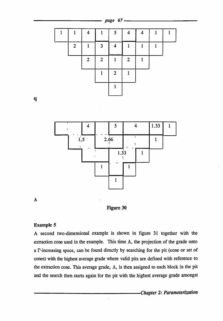
page 67 ------------
1 1 4 1 5 4 4 1 1
2 1 3 4 1 1 1
2 2 1 2 1
1 2 1
1
q
I
4 5 4 1.33 1 I
- . - - --, \ , 1~5 2.66 1 ,
~ \ - "' .... ,
1.33 1 I ,
--1 1
1
A
Figure 30
Example 5
A second two-dimensional example is shown in figure 31 together with the
extraction cone used in the example. This time A, the projection of the grade onto
a r-increasing space, can be found directly by searching for the pit (cone or set of
cones) with the highest average grade where valid pits are defined with reference to
the extraction cone. This average grade, A, is then assigned to each block in the pit
and the search then starts again for the pit with the highest average grade amongst
------------------Chapter 2: Parameterization

--------------------- page 68-----------------------the remaining blocks. In this example, the pits of highest average grade have a value
of 0.60; there are two consisting of one block each, one consisting of four blocks
and one of nine blocks. The largest pit is always chosen. This process is repeated
until the solution shown in figure 31 is found.
1 0.1 0.1 0.3 0.4 0.3 0.2 0.4 0.6 0.4 0.6 0.3 0.2 0.3 0.2 I 0.1 0.2 0.4 0.3 0.4 0.6 0.8 0.8 0.6 0.4 0.2 0.1
0.1 0.2 0.4 0.3 0.5 0.8 0.9 0.4 0.2 0.2
0.2 0.2 0.3 0.3 0.5 0.9 0.5 0.3
0.3 0.5 0.3 0.6 0.8 0.4
0.1 0.2 0.4 0.6
Figure 31(a): two-dimensional example; block grades
I I
X
Figure 31(b): extraction cone r(x) for two-dimensional example
10.16 0.24 0.37 0.40 0.43 0.53 0.60 0.60 0.60 0.60 0.60 0.48 0.40 0.3°1
0.16 0.24 0.37 0.38 0.43 0.53 0.60 0.60 0.60 0.48 0.40 0.30
0.16 0.24 0.37 0.38 0.43 0.53 0.60 0.48 0.40 0.30
0.16 0.24 0.33 0.38 0.43 0.48 0.40 0.30
0.16 0.24 0.33 0.38 0.40 0.30
0.10 0.20 0.33 0.30
Figure 31(c): A values for the example in figure 31(a)
---------------------------------Chapter 2: Parameterization

------------ page 69 ------------
The A values are seen to be r-increasing, i.e. for any given block, the A
values of all blocks within its extraction cone are greater than or equal to the A
value for that block. Thus for any given cut-off value A, the set of blocks defined
by A ~ A constitute a feasible pit. Moreover, every technically optimal pit is
completely defined by a parameter A.
7. Implementation of parameterization
The parameterization algorithm is implemented by using the triangle and spiral
methods. The triangle method is applied to determine the projection of Al onto the
r-increasing space F(fPl' <P2, <P3) using the grade and volume of the selected blocks.
The blocked solution can then be used as an initial function for the spiral method to
find the optimal solution of pits which sa~isfy the constraints of an extraction cone
of triangular base. The same is true for A2 but this time for the r-increasing space
F(fP4' fPS,fP6)
The projections of Al and ~ are obtained by iterative processes which yield
two-dimensional matrices of functions (x,y). The projections are done by assigning
grade and tonnage values to each block and then using the two-dimensional Lerchs
Grossmann algorithm.
The orebody block model is divided into parallel sections and the modified
Lerchs-Grossmann method is applied to each section to determine the optimal shape
of the two-dimensional pit for each level on this section. Thus for each section there
will be an optimum pit limit by level together with the corresponding optimal value.
These values are then accumulated into columns, which determine a two-dimensional
numerical matrix for the pit.
------------------Chapter 2: Parameterization

page 70------------------------When the two-dimensional matrix is found for all sections representing the
pit then a parameterization method is issued to parameterize the two-dimensional
matrix. In this study the search of the matrix is based on the two-dimensional
parameterization algorithm written by Moks (1983) and modified by Dowd (personal
communication). The algorithm is the reverse of the original one. Instead of the
search for the right hand quadrant, Moks saw in his study that the larger pits
corresponding to lower values of grade are of interest and he thus found it desirable
to reverse the solution procedure by defming the lower left hand quadrant, and
searching and removing the pits satisfying the extraction cone of minimum grade.
The two-dimensional matrix is searched for the panel with the minimum
grade for its left hand quadrant. The minimum grade of each quadrant is compared
with that of the previous one; if it is less than the previous one, the two quadrants
are accumulated together and removed. If not, then all the panels are set back to
their original values and the procedure recommences for the next quadrant. The
results of each procedure are stored and compared with the previous one. The final
results are returned to the main program.
During the use of the triangle and spiral methods it sometimes happens, after
a certain number of iterations, that the norm gives only slight changes around a few
pits. In such cases efficiency is improved by stopping the convergence procedure.
The subroutine stack is used in the subroutine projection to control the norm
value for each projection. It is then checked against the following value until the last
iteration of the subroutine (six iterations with six norm values for the triangle
method and only three for the spiral method). If the norm stops increasing or shows
only a few variations around the pits then the solution is blocked.
To ensure convergence of the projection after a finite number of iterations
its progress should be systematically checked. At the end of each projection a
subroutine test is called to check whether the norm values are similar. If so,
--------------------Chapter 2: Parameterization

page 71-----------------------convergence is deemed to have been reached and the procedure is halted; if not, the
procedure continues. The maximum number of iterations is set by the user.
When the pits are found, they are returned to the main program and a
number of characteristic values of each individual pit are calculated. These
characteristic values are:
• the average grade
• the selected tonnage
• the total tonnage
• the quantity of metal
• the stripping ratio and
• the ore-total tonnage ratio.
8. Economic optimization
8.1 Selection of the final pit
Matheron (1975) approaches the economic parameterization very theoretically
and derives the parameterizing function which characterises the optimum for
maximum revenue. The isovalue curves of this function might give the optimum pit
design. The aim of this method was to consider the variability of an optimum pit
when a given economic parameter A changes. For each block the profit value will
appear as a function W(A) of this parameter (monotonic function). This can also be
seen in the paper by Francois-Bongarcon and Marechal (1976).
-----------------Chapter 2: Parameterization

page 72------------------------
In this work the final pit limits have been estimated by methods which are
based upon two factors :
(1) the orebody block model, on which all calculations are based, consists
of values estimated from sparse data and it is thus subject to
uncertainty and error
(2) the cost constraints are applied through what is called a
parameterizing function which is based on both geometrical
constraints and varying economic values.
The objective of the ultimate pit limit design is to detennine the projected
[mal pit limits of an orebody and its associated projected grade and tonnage, which
will maximize some pre-specified economic criteria while satisfying practical
operational requirements.
The parameterization approach enables us to present various alternative pit
designs to the user so that the best plan, as defined by a specific combination of
parameters (mining and processing costs etc ... ) can be selected. This is not possible
with the standard block revenue model approach as applied by such methods as the
original Lerchs-Grossmann algorithm (though it can be handled by the Whittle
(1988) 4-D proprietary software).
The objective is to select the pit that has the maximum net worth attainable
within an acceptable risk range and within any given constraints. For our purposes,
this plan is the optimal plan.
------------------Chapter 2: Parameterization

page 73------------------------8.1.1 Profit matrix
The determination of optimal ultimate pit limits, by nearly all of the computerised
techniques, requires the transformation of the block grade matrix into a revenue
block matrix which can be optimised (scheduled) according to a pre-determined
economic criterion subject to geometric constraints of access.
Block profit comes from the evaluation of a function of many variables such
as grade of ore, mining costs, transportation costs, price of mineral, etc. The net
value for each block is the actual cost or profit realised by mining and processing
a block. Blocks with positive profit have a final value which covers all costs
(mining, production, transport, etc.) whereas negative profit blocks do not.
8.1.2 The general costing equation
The selection of the optimum pit amongst the set of pits produced by the
parameterization method is done by using a simple profit function of the form:
where:
A-(B+C)
A is the revenue from the sale of the finished metal,
B is the total processing cost, and
C is the mining cost.
Clearly A, Band C are all functions and it is assumed that:
(i) all variables affecting profit are included in the functions A, B or C,
and
(ii) blocks of all grades are acceptable for processing. However, very low
grades may give no finished metal, so A = o.
------------------Chapter 2: Parameterization

----------------------- page 74------------------------Clearly:
(i) If A < B then profit < - C. In this case the block would be of very
low grade, regarded as waste and not processed. This gives A = B
= 0 and profit = - c.
(ii) If A > (B + C) then a positive profit is realized from mining and
processing a block regarded as ore.
(iii) If A > B and A < (B + C) then by mining and processing the ore
a loss is incurred but the loss is less than mining with no subsequent
processing. In practice this is marginal ore and is regarded here as
ore.
The cut-off grade is used as a constraint. If the block grade gi is greater than
or equal to the cut -off grade then it is treated as an ore block, if it is less than the
cut-off grade then it is treated as a waste block. Normally, ore blocks have positive
net profit values and waste blocks are negative. The plant cut-off grade is that for
which A = B.
In practice, of course, this representation is too simplistic and it is necessary
to allow for taxation, overheads, capital investment and other financial features.
S.1.3 The optimum pit
Ideally, mining is done in such a manner as to maximize profit throughout the mine
life while maintaining operational continuity. To illustrate the use of the above
formulation the simplest revenue formula is usually of the type:
Pr(i) = A V q(i) - B V - C V if ore q(i) ~ COG
Pr(i) = - C V if waste q(i) < COG
--------------------Chapter 2: Parameterization

page 75 ------------
Where:
Pr(i) is the profit value of block i
q(i) is the grade of block i
COG is the cut -off grade
V is the tonnage of block i
A is the sale price of metal per tonne
B is the processing cost per tonne
C is the mining cost per tonne
For this revenue formula, the implicit assumptions are :
1. The economic values assigned are constant throughout the mine and
throughout the mine life.
2 The profit motive (maximizing revenue) is in use, but without time
discounting.
3. The mining costs are the same for ore and waste.
4. The price is net of transport and marketing costs.
By applying the profit function to each block, a block profit matrix is
generated. Pit profit is obtained by summing the profit of each block that has to be
mined within that pit limit to produce the required profit.
Such a definition (selection) of an optimum pit is taken to be the
configuration of blocks whose pit profit is a maximum.
------------------Chapter 2: Parameterization

page 76 ------------
9. Application of parameterization
9.1 Computer program
The application of the parameterization method and the interpretation of the results
in terms of conventional open pit characteristics require additional work. This extra
work involves the construction of plan, metal inventories and ore-waste ratios for
each pit dermed by a critical cutoff grade. These calculations have been incorporated
into a computer program.
The program which has been used in this study is based on an original coding
by Moks (1983), updated and amended by Dowd, and written in FORTRAN 77. The
original versions have been extended in the current project to include the choice of
the fmal pit and the integration with a scheduling algorithm for more detailed mine
planning. The performance of the software has been improved to enable it to run
faster and more efficiently and in a more interactive manner. The original
parameterization method is retained in the new developments.
9.2 Input and Output
The user provides to the interactive part of the program :
• the cutoff grade, _
• the block dimensions,
• the specific gravity of the ore, -
• the pit wall slope angle --
-----------------Chapter 2: Parameterization

----------------------- page 77--------------------------• the estimated set of data (block grades) stored in a computer file in
3-D form, (including X, Y and Z co-ordinates).
The program then produces a set of nested pit designs (characteristics and
plans), based on the specified input data, at an average of approximately 30 seconds
of computer run time on a Sun workstation. The output is provided in two forms.
The first is a binary file created for efficient storage and data transfer to other
programs (not discussed here). The second file contains full details of the complete
characteristics and plans and a summary of each individual pit. The plans of the
nested pits are given as grade distributions or level heights, both of which can be
used to provide pit contours. The characteristics are those parameters which define
the pits in economic terms such as cash flows.
The characteristics associated with each pit design, such as metal content,
total tonnage, average grade and stripping ratio, are easily calculated and
interpreted. But the most difficult is the representation and the location of the shape
in the form of an open pit design. However, the design of pits is always determined
by boundaries rather than by internal grade distributions and the contour plan is the
better tool for these representations.
9.3 Interpretation and presentation: display of output
A program was written to process the numerical data into graphical output and
produce graphical representations of the characteristics (metal content, total tonnage,
average grade, stripping ratio, etc ... ) of any pit plan. The program was written for
a Sun workstation using graphics routines from the UNlRAS package (1989).
UNlRAS is a software system consisting of a set of subroutines and functions
(UNlRAS Reference and User Manuals) used by an applications program to generate
images and pictures on display input/output devices. The graphics display program
developed in this research project was written in FORTRAN 77, and is designed to
-----------------------------------Chapter 2: Parameterization

page 78-----------------------provide users with the choice of generating the following output:
1- Selection of the final pit
2- Two-Dimensional contouring of mining levels
3- Three-Dimensional representation of the optimum pit plan
4- Cross-sectional representation of pit elevations
5- Three-dimensional views of blocks mined
The graphics display programs will be presented and described more
comprehensively, and examples will be given to illustrate their use, in Chapter 6 of
this thesis.
10. Conclusions
The parameterization method allows the calculation of many optimal pits at the same
time, corresponding to different values of the parameter A . These pits are obtained
without considering economic parameters, and also construct the relationship
between cutoff grade and tonnage, or the quantity of metal and total tonnage of
exploitation. In one computer run, it gives all possible pits of the orebody for a
given parameter A. The user can decide the size of the blocks to be optimised
without creating a problem about the presentation of the results.
The objective of parameterization is to find a complete family of technically
optimal pits corresponding to every possible value of the total tonnage and the
selected tonnage. The crucial assumption for the success of the method is that this
family contains the pit that is optimal for any specified sets of economic parameters.
The only drawback is the limitation on the slope angle of the cone.
------------------Chapter 2: Parameterization

page 79------------------------
However, practical applications of parameterization are not well documented
and some questions remain about the general applicability of the method. It is still
not clear whether there are significant practical cases in which the following may
prevent a true optimum being reached:
1 Approximating the surface found by Qrnaxi (at any T) by the convex
hull Q - AT is likely to miss some pit designs.
2. Approximating the extraction cone by one of polygonal base.
3. The grouping of blocks by their polygonal coordinates into discrete
ordered subsets.
4. The approach to the projection by decomposition and iteration.
5. If used, the imposition of a minimum significant tonnage between
pits.
However, parameterization appears to be at least as good as most algorithms
and better than most in respect of the computing time and, more importantly, the
block model it uses. Even with the introduction of technical parameterization as the
most recent development the problem is not yet solved to everybody's satisfaction.
------------------Chapter 2: Parameterization

CHAPTER THREE
Determination and optimization of mining sequences
Page
1. Introduction 81
1.1 Scheduling as a general problem 81
1.2 Parameterization as a means of scheduling 83
1.3 Simplifying the problem 84
1.4 Pit scheduling 86
1.5 Characteristics of mining sequences 87
1.5.1 Illustration 87
1.5.2 General characteristics 89
1.6 Mining sequence constraints 92
1.6.1 Cone generation 92
2. Optimization of mining sequences using Linear Programming 94
2.1 Introduction 94
2.2 Linear Programming 96
2.2.1 Simplex method for solving mining scheduling
problems 98
2.2.2 Other Linear programming algorithms for solving
mining scheduling problems 104
--------------Chapter 3: Optimal mining sequences

----------------------- page 81------------------------
1. Introduction
A major problem in mine planning and design is the determination of the mining
sequence which will optimize some specified criterion. The criterion of most
interest, especially during feasibility studies, is maximum net present value. Ideally,
the maximum net present value should also be the criterion for the optimal open pit
design. However, as noted in Chapter 2, this involves an intractable circular
argument. The optimal open pit design problem with net present value as the
optimizing criterion could also be viewed as a scheduling problem:
Schedule the mining of the blocks, subject to mining access constraints, in
such a way that the maximum net present value is achieved.
The solution to this problem must also yield the pit shape which has
maximum net present value. However, whilst the problem can be formulated in this
manner and solution algorithms are available (e.g., dynamic programming), the
number of blocks comprising most practical orebody models means that algorithms
are prevented from reaching a solution because of prohibitive storage requirements
or equally prohibitive computing times or a combination of the two.
1.1 Scheduling as a general problem
The problem of scheduling arises in many other applications outside the mining
industry and there is an extensive literature on the subject in many of these non
mining applications.
In general, scheduling problems can be subdivided into two categories
deterministic scheduling and stochastic scheduling.
------------------- Chapter 3: Optimal mining sequences

----------------------- page 82-------------------------The deterministic scheduling approach is to formulate the problem in such
a way that there is only one (deterministic) solution. However, in many applications
the variables have uncertain values and solutions can, or at least should, be
expressed in terms of likelihood or probability. In essence the deterministic approach
assumes that the values of all variables are fIXed and known whereas the stochastic
scheduling approach recognizes and includes the uncertainty on each variable.
A realistic approach to mine scheduling should formulate the problem as a
stochastic scheduling problem. However, in this thesis a deterministic approach has
been adopted mainly because this is seen as an essential first step towards a
stochastic formulation. For example, the linear programming approach described in
the next Chapter could readily be adapted to stochastic linear programming and this
is an area for further work and development of the methods described here.
Deterministic scheduling problems can be subdivided into two further
categories (Garey and Johnson, 1979) :
P-problemsfor which there exist optimal solution algorithms of polynomial
complexity.
NP-hard problems which can only be solved by algorithms of non
polynomial complexity.
There are four major methods applied in the solution of NP-hard problems :
Relaxation
In these approaches the original problem is replaced by a similar one in
which restrictions on one or more parameters have been weakened or relaxed
and/or some additional constraints have eliminated possibilities and reduced
the solution space.
-------------- Chapter 3: Optimal mining sequences

----------------------- page 83-------------------------Approximate optimization
Either a heuristic approach is taken or an existing optimizing algorithm is
assisted by the addition of some heuristic aspects. An example of this
approach in mine design is the modified moving cone method of open pit
optimization.
Optimization by enumeration
This approach enumerates all possibilities and then seeks the optimal
sequence. As such it leads to the true optimal solution. An example of this
approach is dynamic programming as applied, for example, to the mine
scheduling problem. Other examples include branch and bound methods and
iterative methods.
Artificial intelligence approaches
These approaches include expert systems, genetic algorithms and neural
networks. Neural network techniques, in particular, offer the possibility of
reaching optimal or near optimal solutions to the mine scheduling problem.
1.2 Parameterization as a means of scheduling
The parameterization method could be used as a means of scheduling. Each pit in
the nested family generated by the application of the parameterization algorithm
represents a set of blocks of a given average grade. On the assumption that net
profit is directly proportional to grade, sets of blocks arranged in descending order
of grade correspond to sets of blocks that maximize net present value (provided that
the sets are not restricted by size). Consider the two-dimensional example in figure
31 of Chapter 2. Each grade increment could be regarded as a pushback as shown
in figure 32 in which blocks comprising the first few grade increments are shown
by different shadings.
--------------Chapter 3: Optimal mining sequences

----------------------- page 84-------------------------
0.16 0.24 0.37 0.40 IW/.~
Figure 32:
Parameterization results from the example given in figure 31 used as
production schedule that maximizes net present value
The difficulty of course is that the grade increments do not necessarily
coincide with production increments or multiples of such increments and it may not
be possible to satisfy production capacities by blocks belonging to these increments.
Nevertheless, this approach offers the possibility of a good practical approximation.
1.3 Simplifying the problem
In practice the optimal open pit scheduling problem can be significantly reduced in
size simply because it is impractical to schedule a mining operation for more than
relatively short time periods (usually 1 to 2 years maximum and occasionally even
less than 1 year). The reasons for this are:
• Financial variables, especially metal prices, cannot be predicted with
any accuracy beyond this period. Significant changes in metal prices
will have a significant effect on the revenue block model which in
tum will alter the optimal mining sequence.
-------------- Chapter 3: Optimal mining sequences

------------------------ page 85--------------------------• Grade and tonnage values assigned to blocks are only estimates not
true values. These estimates are based on relatively sparse data and
are subject to error. In general, the error decreases as more data
become available and are used in the estimation. In addition, the
estimated grades and tonnages may change significantly as more data
become available. Inevitably, in the initial stages, the most accessible
blocks will be better estimated than those at greater depth. As mining
progresses, more data will become available and the revenue block
model may change significantly.
• Many other variables and factors may change throughout the life of
the mine. Such variables include geotechnical properties and
conditions which may affect wall slopes (and hence the mining access
constraints) .
Given these restrictions on the time period over which scheduling can
realistically be applied a sensible approach is :
1 Design an optimal open pit on the basis of any of the common
optimizing criteria (maximum total undiscounted revenue or
maximum metal recovery). This pit defines an outer shell within
which all scheduling (and therefore mining) will be done. This pit
also defines total minable reserves.
2 Schedule blocks within the pit shell over specified scheduling periods
updating the schedule over time and/or as the values of significant
variables (e.g., financial, geological, geotechnical) change.
In certain circumstances, developments during any scheduling period may
require the re-definition of the optimum pit. This feature has not been addressed in
this thesis and remains an important issue to be tackled if the work continues.
-------------- Chapter 3: Optimal mining sequences

----------------------- page 86------------------------
1.4 Pit scheduling
Unlike the problem of determining optimal open pit limits, there are very few
references available which address the subject of pit sequencing in a practical way.
Those papers which do cover the subject recognize the fact that orebodies are
normally mined in stages or sequences. The principles behind open pit mine
scheduling were first clearly stated by Lerchs and Grossmann (1965) :
The same optimal open pit limits could be reached by a multitude of mining
sequences each of which will produce a different cash flow. Therefore there
exists an optimum mining sequence which can be defined as that sequence
which maximizes the present wonh of the deposit. The possible sequences
from which to choose from are of course limited by various constraints
imposed by pit wall stability, the ore requirements of the mill and good
mining practice. The optimum pit limits, therefore, cannot be defined without
first determining an optimum '!lining sequence.
The basis of the most commonly accepted methodology and its underlying
philosophy are discussed in a number of papers and textbooks, most notably, Lerchs
and Grossmann (1965), Roman (1973), Dowd (1976), Wilke and Reimer (1979),
Wilke, Mueller and Wright (1984), Huang (1993), Fytas, Hadjigeorgiou and Collins
(1993).
A new approach, which the author has called the 'combination of linear
programming and simulated, user-activated waste stripping' method, has been
developed as part of this PhD research project. The method consists of three parts: r
waste stripping, linear programming and simulation modules.
These references are used to introduce the general concepts of the method
that forms the fundamental basis of the present and the following Chapter.
------------------Chapter 3: Optimal mining sequences
----------------------- page 87-------------------------The algorithms have been developed for complete three-dimensional
implementation although they could equally well be applied to two-dimensional cases
(e.g., strips of mineable material). The algorithm has been used for a three
dimensional case study and the results have been validated; part of this case study
is given in Chapter 6.
1.5 Characteristics of mining sequences
As mentioned earlier the optimization procedure is required to select the material to
be mined in each sequence of a mining period, to maximize the output at the early
stages, that is to quickly reach the rich ore of the technically optimum pit. This will
maximize the chosen fmancial objective over the life of the mine, satisfying a
carefully selected set of operational constraints. However, mining could proceed
along unlimited alternate paths each of which would generate a unique cash flow
pattern. The path with the highest discounted cash flow should be selected as the
best mining sequence.
The following simple example, taken from Gnur and Dowd (1993), illustrates
the general concepts raised in the previous paragraph.
1.5.1 Illustration
The simple example shown in figure 33 illustrates the importance of net present
value in the detennination of mining sequences. In this example the same section of
an orebody is depleted in the same time period with a discount rate of 10% by using
two different planning sequences. The results are shown in table 1.
--------------- Chapter 3: Optimal mining sequences

----------------------- page 88------------------------
_ mining pwh backs mining pwhbacka -
Figure 33 : two possible mining sequences
It can be seen from table 1 that the best way of mining the orebody is to
mine the most profitable parts during the early stages of the mining operation. The
same results are presented graphically in figure 34.
Time Alternative 1 Alternative 2 Discount Discounted Discounted
period Profit Profit Rate Alternative 1 Alternative 2
1 100 60 0.909 90.9 54.4
2 90 70 0.826 74.3 57.8
3 80 80 0.751 60.1 60.1
4 70 90 0.683 47.8 61.5
5 60 100 0.621 37.3 62.1
Total 400 400 310.4 296.0
Table 1 : Discounted cash flows from two mining sequences
------------------------ Chapter 3: Optimal mining sequences

----------------------- page 89-------------------------
100 I--------------~-L-eg-en-d---,
i 0 Akernative 1
80 +- f-------------i IllllJ Alternative 2
~ ::l C
~ 60 !
~ § 40
£5
20 '
2 3 5 Time period
Figure 34: graphical form of results in table 1
1.5.2 General characteristics
Long range production scheduling is mainly concerned with such criteria as ore
reserves, stripping ratios and major investment usually on a year by year basis.
Short range scheduling, on the other hand, is the development of a sequence of
depletion schedules on a daily, weekly or monthly basis, which complies with
restrictions imposed by the long range plans, plant capacities, inventories, equipment
availability and the existing mining operation.
Regardless of the type of ore or mineral product mined, there are certain
basic data that are required in any production scheduling problem. These are :
1) the tonnage and grade of each block
2) specific gravity of ore and waste
3) the revenue value of each block
4) deposit block model
5) present pitl quarry layout or overall optimum limits of the pitl quarry
-----------------Chapter 3: Optimal mining sequences
-----------------------page 90------------------------to be scheduled,
6) mine life or production rate (depending on whether short term or long
term scheduling is used)
7) the maximum and minimum allowable grade to be mined or to be fed
to the processing plant in any time period
8) maximum and minimum allowable production rate of waste and ore
9) working slope angle in the pit
10) minimum pit bottom dimensions
11) discount rate
12) preproduction rate and period, (if required)
Because of the large number of blocks in most orebody block models it is not
practical to optimize a schedule which simultaneously includes the entire model
covering all periods of the mine life and all types of mining constraints. For this
reason the scheduling problem has been divided into a set of sequential sub
problems. The two major divisions are for time and mining constraints. These
divisions can be summarized as :
Time
The scheduling process proceeds one mine period at a time, and
Constraints
Within each time period the constraints are treated in two major classes.
The simulation
This part handles the physical constraints and forms the main subject of the
present Chapter.
The Linear Programming technique
This part handles the production constraints and parameters and is the main
subject of Chapter 4.
-------------------------- Chapter 3: Optimal mining sequences
----------------------- page 91------------------------The blocks to be mined in each mining period are selected subject to the
given mining access constraints. The constraints on the possible mining sequences
include both physical constraints on the mining operation and economical constraints.
Only the physical constraints are dealt with here.
The following is a list of the operating constraints used in this application and
which the computer program attempts to satisfy :
1. Mining access constraints. These constraints define the access to each
block within the orebody block model. In their simplest form these
constraints prevent the mining of a block which is directly under
another unmined block and prevent the mining of a block for which
any adjacent block has an unmined block above it; in this version
mining must be done in a step-wise manner.
2. The one-for-one restriction requires that for every unit volume which
is mined from a block that is restricted by a number of other blocks,
at least an equal volume must be removed from each of the restricting
blocks.
3. Maximum working slope angle.
4. Minimum radius of a mining area. This constraint is used to impose
access for mining equipment to mining blocks and may include such
specifications as minimum truck turning circle and minimum
allowable access for loaders.
----------------------------- Chapter 3: Optimal mining sequences

----------------------- page 92------------------------1.6 Mining sequence constraints
Determination of an allowable mining sequence is primarily a problem of geometry.
In an actual mining operation the material is removed in such a way that the safe
wall slope is never exceeded in any direction. The practice of benching gives the
open pit mine a step-like structure. These conditions justify the representation of the
outline of a mining plan or the volume of the mineral to be removed, consistent with
the wall slope constraints and mining practices, by a series of frustums.
Given the block size, two methods are used to describe the allowable mining
sequence relative to the block concept; one is to use a cone to define the set of
allowable or required blocks, Erickson and Pana (1966) and the other is to use a
pattern or set of blocks which closely approximates a thin frustum to define the
allowable set Johnson (1968). The second method will be used in the mathematical
formulation given in this Chapter.
1.6.1 Cone generation
A cone (or pit) is generated by the removal of whole blocks from the block matrix.
As a pit is mined, the slope of the sides must not exceed the angle of failure and
a maximum pit slope must be defined and observed. The pit slope considered here
is the average slope generated by a step pattern (as whole blocks are removed).
Thus, considering different step patterns amounts to considering different slopes.
Many other authors have considered cone generation, for example, Boyce
(1969), Hartman, et al (1966), Johnson (1968), Lerchs and Grossmann (1965). The
method adopted here is that of forming a cone with a single block as a base. Two
methods are illustrated, both using cubic blocks. Due to the symmetry and uniform
grid considerations, this requires that alternative benches must have the closest five
blocks in the case illustrated in figure 35a, and the closest nine blocks in the case
illustrated in figure 35b, mined in the bench above before the bench can be opened.
--------------Chapter 3: Optimal mining sequences

----------------------- page 93------------------------
fiQ. 358 - 5:1 fia. 35b - 9:1
Figure 35
The 9: 1 configuration method produces a cone with slopes ranging from 35 0 to 45 0•
The 5:1 configuration method produces a cone with slopes ranging from 45 0 to 55°.
By changing the dimensions of the blocks, i.e. height and width, the slope
produced by the various methods changes and it should be possible in most instances
to arrive at block dimensions and a cone generation procedure which will produce
a close enough approximation to the required pit slope. Block dimensions must,
however, be kept to reasonable size.
For convenience, the block height is generally the bench height of the pit but
the horizontal dimensions are often completely arbitrary. If the size of the block is
large, however, model coarseness can cause the orebody to be completely
misrepresented in terms of recoverable ore.
In attempts to achieve greater precision there is a tendency to reduce the size
of the block, but this is usually restricted to some extent by the drill hole spacing
and possibly by the interpolation (estimation) procedure used. For a given area, the
block size affects the size of the block matrix directly, and hence the storage size
and the amount of computing time required by the program. In other words,
accuracy requires small blocks whereas computing economy is achieved with large
ones; however, the over-riding determinant of block size may be the drilling or
sampling grid.
--------------Chapter 3: Optimal mining sequences

----------------------- page 94-------------------------
2. Optimization of mining sequences using linear • programnnng
2.1 Introduction
In recent years several people have worked on the optimal open pit design problem
as a means of fmding the optimum mining schedule. The optimization criteria vary
with application but are usually based on Net Present Value (NPV) or Maximum
Total Return.
The optimum schedule depends on both physical and economic parameters
which can be considered either together or separately. Considering both parameters
at the same time is computationally time consuming and, for large problems, as the
number of states increases, the solution may be impossible to attain.
The problem can be split into two parts. One part uses Linear Programming
(LP) to find the optimum path, whilst the second part checks the feasibility of the
fIrst solution in terms of mining constraints and improves the scheduling sequence.
The effect of this check is that the final LP solution will always be confined to
blocks which become accessible during the period under consideration.
The idea of free-ore develops the above consideration further. By submitting
for LP selection only those blocks which are immediately available for mining, the
constraints on precedence and accessibility of blocks will be eliminated. Such an
approach cannot lead to a rigorous overall optimum in the mathematical sense.
However, the mining constraints, which play the major role in the definition of the
open pit mine design, are chosen only to constrain the practicability of the solution.
--------------Chapter 3: Optimal mining sequences

----------------------- page 95------------------------
In contrast, the use of combinations of different mining constraints in one
algorithm throughout the scheduling will make the long-term project much more
flexible especially for quick decision making in the case of unforeseen
circumstances, such as unexpected sudden changes in ore (waste), or equipment
break-down etc.
Scheduling is mainly a combination of the physical restrictions and the
economic parameters as discussed above, which usually produce optimum results in
terms of material extracted or in monetary return. Different people have different
ideas on how to achieve this goal.
From the above analysis the scheduling model considered here is divided into
three parts:
1 Waste stripping module.
This deals only with waste and overburden to be mined to expose ore blocks.
2 Linear programming module.
This deals mainly with the ore blocks to be mined .
3 Simulation module
This deals with the re-adjustment of sets of blocks submitted to the LP
module.
The approach used to solve the problem is a combination of Linear
Programming and simulated, user-activated waste stripping with the overall objective
of maximizing the profit or the Net Present Value (total discounted profit).
The pit limits part is done independently of the second (scheduling) using all
combinations which satisfy the mining constraints to give the maximum number of
---------------- Chapter 3: Optimal mining sequences
----------------------- page 96-------------------------combinations of blocks that can be mined during a given period of time. This part
has already been described in Chapter 2.
This approach is the main subject of the next Chapter and deals with the
mining schedule of the material within the optimum open pit limit obtained by the
methods described in Chapter 2.
2.2 Linear programming
During recent years it has become increasingly apparent that operational
research and the use of computers can greatly improve mine planning and increase
the possibility of attaining the management's ultimate goal of total maximum profit.
The operational research technique which has been applied to more production
scheduling problems than any other is Linear Programming (LP).
LP is a mathematical method for determining the optimum allocation of
limited resources to products or activities e.g. the determination of an optimum
production mix or the number of items produced to maximize profit or minimize
costs. The objective is either to maximize the benefits while using limited resources
or to minimize costs while meeting certain requirements.
All linear programming problems have three common characteristics :
1 - A linear objective function: maximize, minimize or equalize z
where:
This is a mathematical statement of what management wishes to achieve.
This could be a statement concerning maximizing profit or minimizing cost.
-------------- Chapter 3: Optimal mining sequences

----------------------- page 97------------------------2 - A set of linear constraints :
The constraints are the physical limitations on the objective function caused
by factors such as budgets, labour, raw materials etc. Linearity means that the
constraints are linear and have flXed coefficients.
3 - A set of non-negative constraints:
with i=1. .. n
This limits the solution to positive (or zero) values of the variables.
Where z = objective function
a = coefficient matrix
b = vector of constraint right-hand-side (RHS)
x = vector of variables
In all linear programming problems there is a set of possible answers all of
which satisfy the constraints. These answers constitute the feasible region. LP then
finds a point in the feasible region which optimises the objective function.
--------------Chapter 3: Optimal mining sequences
----------------------- page 98-------------------------
LP problems are usually solved by a technique known as the Simplex
Method, frrst developed in the 1940's. This method works by taking a sequence of
square sub-matrices of "a" and solving for "x", in such a way that successive
solutions always improve, until a point in the algorithm is reached where
improvement is no longer possible. The method is used in this work and is further
explained in sub-section 2.2.1.
2.2.1 Simplex method for solving mining scheduling problems
We frrst need to specify the objective function in standard form, and convert all the
inequalities to equations. Having specified the problem we convert the inequalities
to equations by adding non-negative slack variables. The slack variables represent
any unused capacity in the constraint . Each constraint will have its own slack
variable.
For example: 3Xl + 4X2 < 50 becomes 3Xl + 4X2 + XJ = 50 where : X3 ~ 0
The slack variable represents any unused capacity in the constraint and in this
case 0 < X3 < 50. Where x 3 = 50 represents the case of zero production and
X3 = 0 represents the case of full utilisation of the resources and zero unused
capacity. Each constraint will have its own slack variable.
The Simplex method is a step by step arithmetic method of solving LP
problems whereby one moves from a position of zero contribution until no further
contribution can be made. Each step produces a feasible solution and an answer
which is better than the previous one. The method is better explained in the
following example.
--------------Chapter 3: Optimal mining sequences

----------------------- page 99------------------------
Maximize the following linear objective function :
z = 8x 1 + 5X2 + lOx 3
Subject to the linear constraints :
2XI + 3x2 + X3 < 400
Xl + X3 < 150
2Xl + 4X3 S 200
X2 S 50
And the non-negativity constraints:
Solving the above example first we add the slack variables,
=400
= 150
+ ~ = 200
+ X7 = 50
with Xi ~ 0 and i = 1... 7
Writing the objective function in' standard form: z - 8x1 - 5x2 - 10Xj = 0
and then the simplex tableau takes the form:
------------------------ Chapter 3: Optimal mining sequences
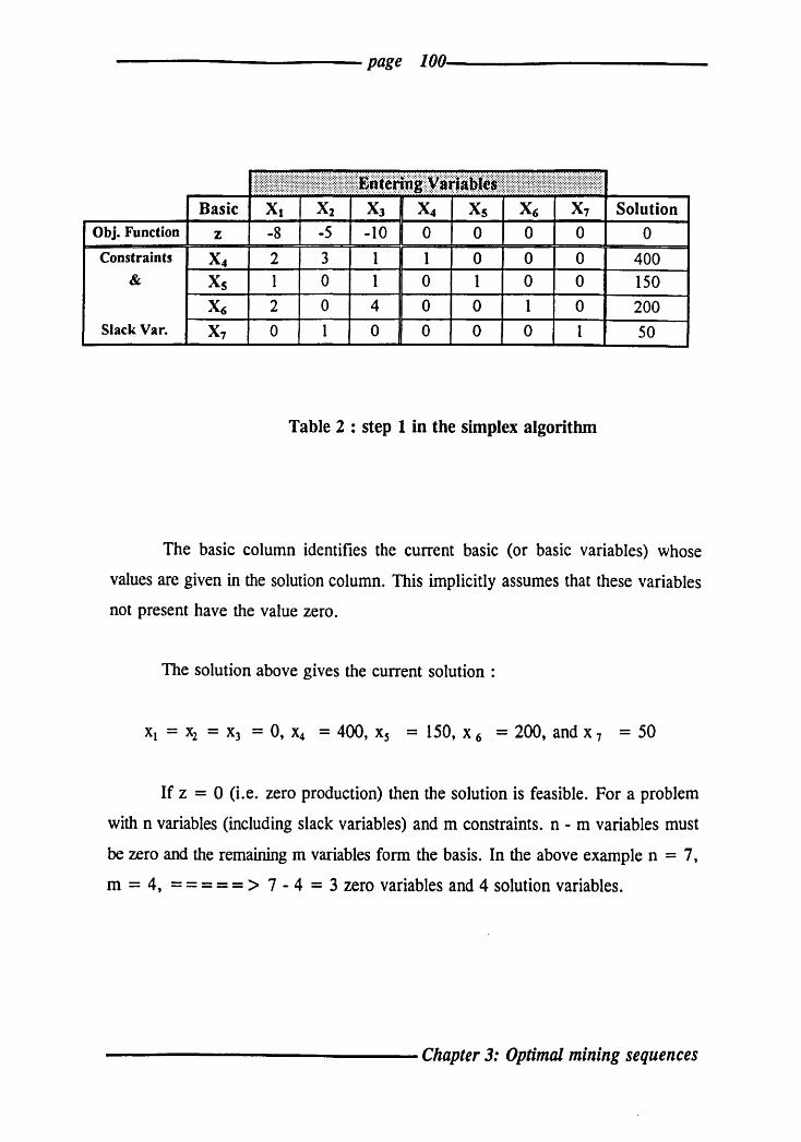
---------------------page 100-----------------------
Obj. Function
Constraints
&
Slack Var.
Basic
z
X4
Xs X, X,
Xl -8
2
I
2
0
Xl Xl X4 Xs X, X, Solution
-5 -10 0 0 0 0 0
3 1 1 0 0 0 400 0 1 0 1 0 0 150
0 4 0 0 1 0 200
I 0 0 0 0 50
Table 2 : step 1 in the simplex algorithm
The basic column identifies the current basic (or basic variables) whose
values are given in the solution column. This implicitly assumes that these variables
not present have the value zero.
The solution above gives the current solution :
Xl = X2 = X3 = 0, X4 = 400, Xs = 150, X 6 = 200, and X 7 = 50
If z = 0 (Le. zero production) then the solution is feasible. For a problem
with n variables (including slack variables) and m constraints. n - m variables must
be zero and the remaining m variables fonn the basis. In the above example n = 7,
m = 4, = = = = = > 7 - 4 = 3 zero variables and 4 solution variables.
---------------- Chapter 3: Optimal mining sequences
------------ page 101-------------
If we examine the current zero variables (xh x 2 and X3) all have negative
coefficients (-8x.-5x2-10x3) which is equivalent to positive coefficients in the original
objective function (8Xl +5X2+ 10x3). Since we are maximizing, the value of z can be
increased by increasing Xl' X2 or X, above the zero value. However, we always select
the variable with the most negative objective coefficient because such a solution is
most likely to lead to the optimum solution rapidly (Le. coefficient of x3).
The optimality condition is, in the case of maximization, i.e. (-8-5-10) = = >
(0, 0, 0). If all non-basic variables have non-negative values in the z equation in the
current tableau, the current solution is optimal. Otherwise the non-basic variable
with the most negative coefficient is selected as the variable entering the basis.
The feasibility condition determines which variable leaves the basis, this
variable is the one which will be first to reach zero when the entering variable
reaches its maximum value. It is identified by dividing the solution value by the
corresponding positive values in the column of the variables entering the basis. The
row with the smallest value identifies the variable leaving the basis.
The algorithm for the above method proceeds as follows:
Step 1. Identify the largest negative value in the z-row (Le. -10)
Step 2. Divide the solution quantity by the positive values in this column.
(Le. 400/1, 150/1, 200/4)
Step 3. Select the row which has the element with the smallest positive value
(200/4 = 50) and identify the value that appears in both the row and
the column. This element is the PIVOT element (Le. 4).
Step 4. Divide all the elements in the row by the pivot and replace the basic
variable by the entering variable. In this case X6 is replaced by x 3 •
--------------Chapter 3: Optimal mining sequences

-----------page 102------------
The new pivot equation is equal to the old pivot equation divided by the pivot
element (Le. new pivot equation).
The new pivot equation is :
Xl Xl Xl X4 Xs X6 X7 Solution
I Xl Yi 0 1 0 0 Y4 0 50
Step S. Using row operations (Gauss-Jordan method) make all other elements
in this column zero using the PIVOT row.
Iteration Basic Xl Xl Xl X4 Xs X6 X7 Solution
1 z -3 -5 0 0 0 2Yi 0 500
Xl enters X4 lYi 3 0 1 0 -Y4 0 350
Xs Y2 0 0 0 1 -Y4 0 100
X6 leaves Xl Y2 0 1 0 0 Y4 0 50
X, 0 1 0 0 0 0 1 50
Table 3 : step 5 in the simplex algorithm
---------------Chapter 3: Optimal mining sequences
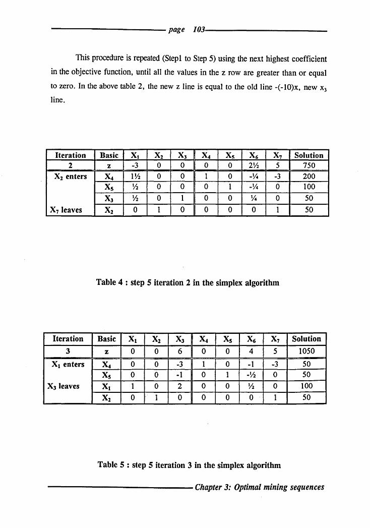
------------page 103------------
This procedure is repeated (Step 1 to Step 5) using the next highest coefficient
in the objective function, until all the values in the z row are greater than or equal
to zero. In the above table 2, the new z line is equal to the old line -( -lO)x, new X3
line.
Iteration Basic Xl X2 X3 X4 X5 X6 X7 Solution 2 z -3 0 0 0 0 2Y2 5 750
Xl enters X4 lY2 0 0 1 0 -v.- -3 200
X5 Yl 0 0 0 1 -v.- 0 100
Xl Yl 0 1 0 0 v.- 0 50
X, leaves X2 0 1 0 0 0 0 1 50
Table 4 : step 5 iteration 2 in the simplex algorithm
Iteration Basic Xl Xl Xl X4 Xs X6 X7 Solution
3 z 0 0 6 0 0 4 5 1050
Xl enters X4 0 0 -3 1 0 -1 -3 50
Xs 0 0 -1 0 1 -Yl 0 50
Xl leaves Xl 1 0 2 0 0 Yl 0 100
Xl 0 1 0 0 0 0 1 50
Table 5 : step 5 iteration 3 in the simplex algorithm
--------------- Chapter 3: Optimal mining sequences

-----------------------page 104------------------------
As all quantities in the z-row are greater than or equal to zero we have
reached the optimum.
i.e. Xl = 100, X2 = 50, X 3 = 0, X 4 = 50, X 5 = 50, x 6 = ° and
x 7 = 0, with a maximum profit of : z = 1050.
In minimisation problems the entering variable must have the largest
positive coefficients in the z equation. The solution is reached when all the values
in the z row are less than or equal to zero and the non-basic variables have non
positive coefficients.
2.2.2 Other LP algorithms for solving mining scheduling problems
Other LP algorithms known as Interior-Point methods come from non-linear
programming approaches proposed in 1958 and further developed in the late 80's.
These methods can be faster for many large-scale problems. Such methods are
characterized by constructing a sequence of trial solutions that go through the
interior of the solution space, in contrast to the Simplex Method which stays on the
boundary and examines only the comers (vertices).
Integer LP models are ones where the answers must not take fractional
values. Integer models may be ones where only some of the variables are to be
integer and others may be real-valued termed Mixed Integer Linear Programming
(MILP), or Mixed Integer Programming (MIP); or they may be ones where all the
variables must be integer termed Integer Linear Programming (ILP). The class of
ILP is often further subdivided into problems where the only legal values are Binary
(0,1), and general integer problems.
------------------------- Chapter 3: Optimal mining sequences

----------------------page 105----------------------
Although various algorithms for MIP have been studied, most if not all
available general purpose large-scale MIP codes use a method called 'Branch and
Bound' to try to fmd an optimal solution. Branch and Bound solves MIP by solving
a sequence of related LP models. Good codes for MIP distinguish themselves more
by solving shorter sequences of LP's, than by solving the individual LP's faster.
Even more so than with regular LP, a costly commercial code may prove its value
if the MIP model is difficult.
There are certain models whose LP solution always turns out to be integer,
assuming the input data is integer to start with. The theory of unimodular matrices
is fundamental here (unimodular is: if every square sub-matrix has a determinant
equal to 0, + 1, or -1). Such problems are best solved by specialized routines that
take major shortcuts in the Simplex Method, and as a result are relatively quick
running compared to ordinary LP.
Nowadays, with good commercial software, models with a few thousand
constraints and several thousand variables can be tackled on a 386 PC. Workstations
can often handle models with variables in the tens of thousands, or even more, and
mainframes can go larger.
The choice of code can make more difference than the choice of computer
hardware. It is hard to be specific about model sizes and speed, a priori, due to the
wide variation in things like model structure and variation in factorizing the basis
matrices; just because a given code has solved a model of a certain dimension, it
may not be able to solve all models of the same size, or in the same amount of time.
For the application of LP to the Mining Scheduling Problem, a code, written
in "C" language, called lp_solve was supplied to the author by Proll (1995).
Lp _solve can solve general LP problems or mixed integer LPs. The code uses a
Simplex Algorithm and sparse matrix techniques, for pure LP problems. If one or
more of the variables is declared integer, then the simplex algorithm is iterated with
---------------Chapter 3: Optimal mining sequences
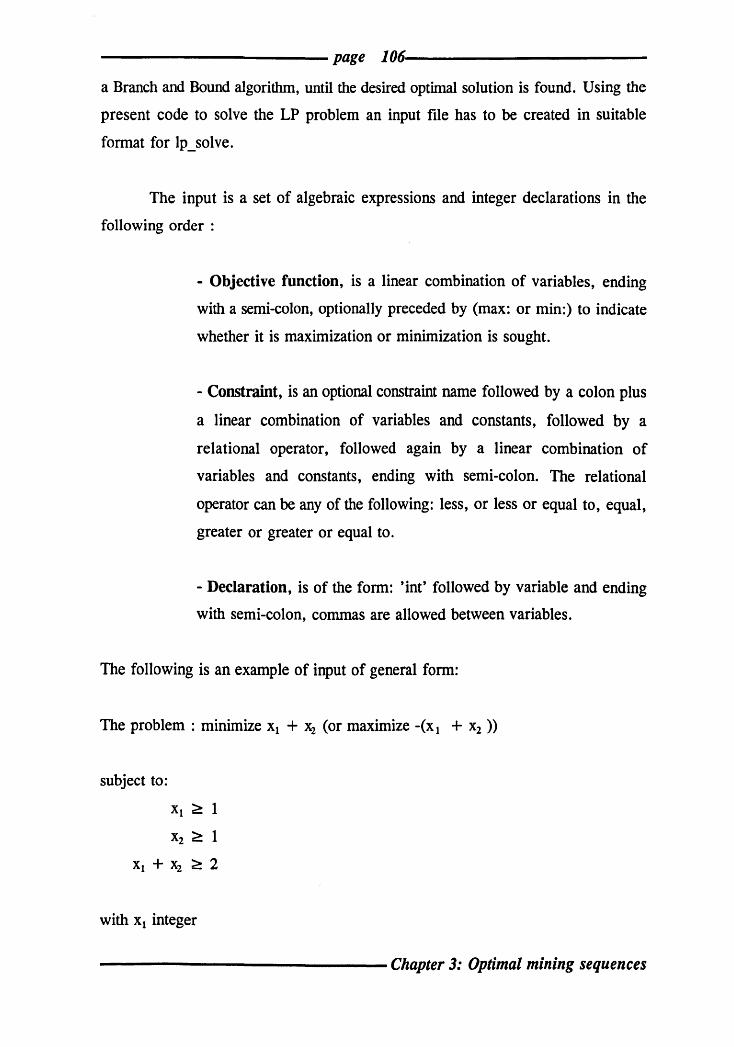
----------------------page 106------------------------
a Branch and Bound algorithm, until the desired optimal solution is found. Using the
present code to solve the LP problem an input file has to be created in suitable
format for lp_solve.
The input is a set of algebraic expressions and integer declarations in the
following order :
- Objective function, is a linear combination of variables, ending
with a semi-colon, optionally preceded by (max: or min:) to indicate
whether it is maximization or minimization is sought.
- Constraint, is an optional constraint name followed by a colon plus
a linear combination of variables and constants, followed by a
relational operator, followed again by a linear combination of
variables and constants, ending with semi-colon. The relational
operator can be any of the following: less, or less or equal to, equal,
greater or greater or equal to.
- Declaration, is of the form: 'int' followed by variable and ending
with semi-colon, commas are allowed between variables.
The following is an example of input of general form:
The problem: minimize Xl + X2 (or maximize -(Xl + X2 »
subject to:
Xl ~ 1
X2 ~ 1
Xl + x2 ~ 2
with Xl integer
---------------Chapter 3: Optimal mining sequences

------------ page 10'/.------------
The lp_solve input file is:
max: -Xl + -X2;
(or min: Xl + x2 ;)
Xl ~ 1;
x2 > 1;
Xl + X2 ~ 2;
int Xl;
The results from Lp _solve are the values of the decision variables, that
represent the status of the blocks, together with the profit gained from mining that
set of blocks. The values of the decision variables are 0 (for blocks not mined) and
1 (for mined blocks) in any given time period examined. More details are given in
Chapter 6.
The software is unlimited in size but the computer platform on which it is
implemented sets upper limits to the size of the problems that can be practically
solved.
---------------Chapter 3: Optimal mining sequences

CHAPTER FOUR
Optimal production scheduling in open pit operations
1. Introduction
2. Linear programming
Page
109
109
3. Practical solutions: reducing the numbers of constraints and variables 111
4. The model
5. The waste stripping module
6. The linear programming module
7. The mining simulation module
8. Solving the linear program
8.1 Additional constraints
9. Conclusion
112
113
115
118
119
120
120
------------ Chapter 4: Optimal production scheduling

page 109------------------------
1. Introduction
The production scheduling problem can be stated simply as the determination of the
sequence in which blocks must be mined, subject to mining, economic and
geotechnical constraints, so as to optimize a specified objective function.
In this application the objective is to maximize the net present value of the
total mined product. The author uses a combination of linear programming and
simulated, user-activated waste stripping to obtain the optimum schedule.
2. Linear programming
To illustrate the linear programming
formulation assume that the blocks in
the block model are regular cubes and
that the pit slope constraints are 45° in
all directions. It is further assumed that
the pit slope constraints also define the
mining access constraints as illustrated
in figure 36 in which the lower block
can only be mined in a given period if.
the nine blocks on the level above have
I I I
~ Figure 36:
illustration of mining constraints
been mined in previous periods and/or are mined in the given period. This simplistic
example does not in any way constrict the generality of the formulation which
follows.
Let bijk(t) be a binary valued variable which takes the value 1 if block (i,j,k)
is mined in period t and takes the value 0 otherwise. The indices i,j,k are block
counters in the east-west (x), north-south (y) and vertical (z) directions respectively
Chapter 4: Optimal production scheduling
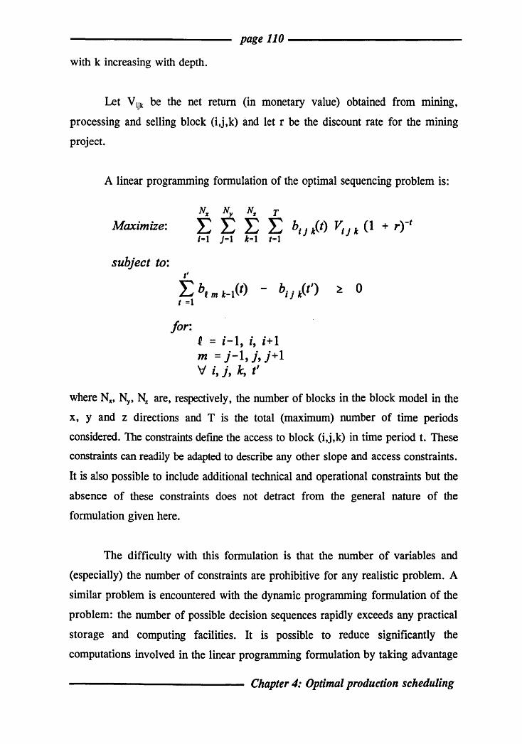
page 110-----------------------
with k increasing with depth.
Let Vijk be the net return (in monetary value) obtained from mining,
processing and selling block (i,j,k) and let r be the discount rate for the mining
project.
A linear programming formulation of the optimal sequencing problem is:
Maximize:
subject to: t'
L h. m 1-1(t) - bi } 1(t') ~ 0 t =1
for: ~ = i-I, i, i + 1 m =j-l,j,j+1 \;f i, j, k, t'
where Nx, Ny, Nz are, respectively, the number of blocks in the block model in the
x, y and z directions and T is the total (maximum) number of time periods
considered. The constraints defme the access to block (i,j ,k) in time period t. These
constraints can readily be adapted to describe any other slope and access constraints.
It is also possible to include additional technical and operational constraints but the
absence of these constraints does not detract from the general nature of the
formulation given here.
The difficulty with this formulation is that the number of variables and
(especially) the number of constraints are prohibitive for any realistic problem. A
similar problem is encountered with the dynamic programming formulation of the
problem: the number of possible decision sequences rapidly exceeds any practical
storage and computing facilities. It is possible to reduce significantly the
computations involved in the linear programming formulation by taking advantage
--------------- Chapter 4: Optimal production scheduling

page 111 --------------------------
of the properties of the unimodular matrix formed by the constraints and by using
various algorithmic approaches that are well documented in the linear and integer
programming literature. However, the linear program, as formulated above, is still
too large to be solved for all but the smallest of block models.
Some authors (Wilke and Reimer (1979), Wilke et. al. (1984) and Huang
(1993)) have attempted to separate the access constraints from the linear program but
it is intuitively obvious (and easy to demonstrate) that such approaches cannot
possibly lead to optimal solutions in any problem that involves sequential decisions.
In all but the simplest cases they do not even lead to near optimal solutions and thus
the use of such simplifications is a dangerous approach to optimal scheduling.
3. Practical solutions: reducing the numbers of constraints and
variables
It is possible to adapt the linear programming formulation by recognising some
subtle differences between optimal open pit design and the optimal sequencing of
mining blocks and by recognising that the solution yielded by any general
formulation will not necessarily be a practical mining solution:
(1) An initial pit will always be
designed well in advance of any
need to schedule the mining
operation: scheduling can be seen as
the order In which blocks are
removed so as to reach an ultimate
pit shape.
(2) Mining generally proceeds in fronts Figure 37:
simplified block access for scheduling
Chapter 4: Optimal production scheduling

page 112 -----------
and mining access to a particular block is not as stringent as that required for
pit design. For example, mining is usually done by "push backs" on benches
and, in its simplest form, access could be defined in terms of one block
above and one block in front as shown in figure 37.
(3) Blocks that are already accessible do not require an access constraint.
(4) For technical and economic reasons blocks must be mined (more or less)
contiguously in groups. In general it is not feasible, or at least not good
mining practice, to mine isolated blocks in different parts of the orebody.
Similarly, mining will not be done on a large number of widely separated
levels in any given period or even over short to medium sequences of
consecutive periods; the number of levels opened and the distance between
them will usually be restricted.
(5) Scheduling for any practical purposes is very rarely considered for more than
relatively short periods of time (3 to 5 years maximum)
4. The model
The approach adopted here is similar in structure to that of Huang (1993). There are
three components in the model:
(1) A user-activated waste stripping module.
(2) A linear programming module that determines an optimal mining
sequence from sub-sets of blocks submitted from the overall orebody
block model.
Chapter 4: Optimal production scheduling

page 113 ------------
(3) A mining simulator which removes mined blocks from the block
model and adjusts the subsets of blocks for submission to the linear
programming module.
It is assumed that an overall pit has already been designed (in this work by
means of the parameterization algorithm). This is not an essential requirement but
it does simplify the procedure. It is further assumed that a minimum amount of ore
must always be exposed in any given time period. This is a fairly widespread and
sensible operational requirement. Before production begins, for example, a certain
amount of overburden and/or waste must be stripped. The final assumptions are for
access to blocks:
(I) access to any block in the uppermost layer of the orebody block
model is determined solely by removal of the waste block
immediately above it.
(2) for all other layers in the orebody block model an accessible block
(i,j,k) is one for which the block immediately above (i,j,k-l) has been
removed and at least one contiguous block on the upper level has
been removed: (i-l,j,k-l) or (i,j-l,k-l) or (i,j + I,k-I) or (i + I,j,k-I).
5. The waste stripping module
A minimum tonnage of ore must be exposed at the start of each period. This
minimum tonnage is specified by the user and is determined by the program in terms
of numbers of accessible are blocks.
The minimum exposed are tonnage constraint is a common production
------------ Chapter 4: Optimal production scheduling

page 114 ------------
requirement and, in this application, is a valuable means of reducing the number of
constraints for the linear programming module.
on:
All ore blocks that are not accessible are assigned a priority code depending
(1) The number of faces of the block (if any) that are already
exposed.
(2) The value of the block.
In descending order of priority each ore block is then examined to determine
whether access is prevented by a waste block. If so, the waste block is scheduled for
removal. Stripping continues until the minimum tonnage of ore is exposed. Apart
from any pre-production stripping, all waste stripping incurred by this module is
apportioned equally over the periods considered by the linear programming module
and capacity constraints are adjusted accordingly.
At any stage the user can intervene to identify specific blocks to be stripped.
This option can be used to override part or all of the automatic stripping operation.
When the minimum amount of ore tonnage is exposed control passes to the
linear programming module.
Chapter 4: Optimal production scheduling
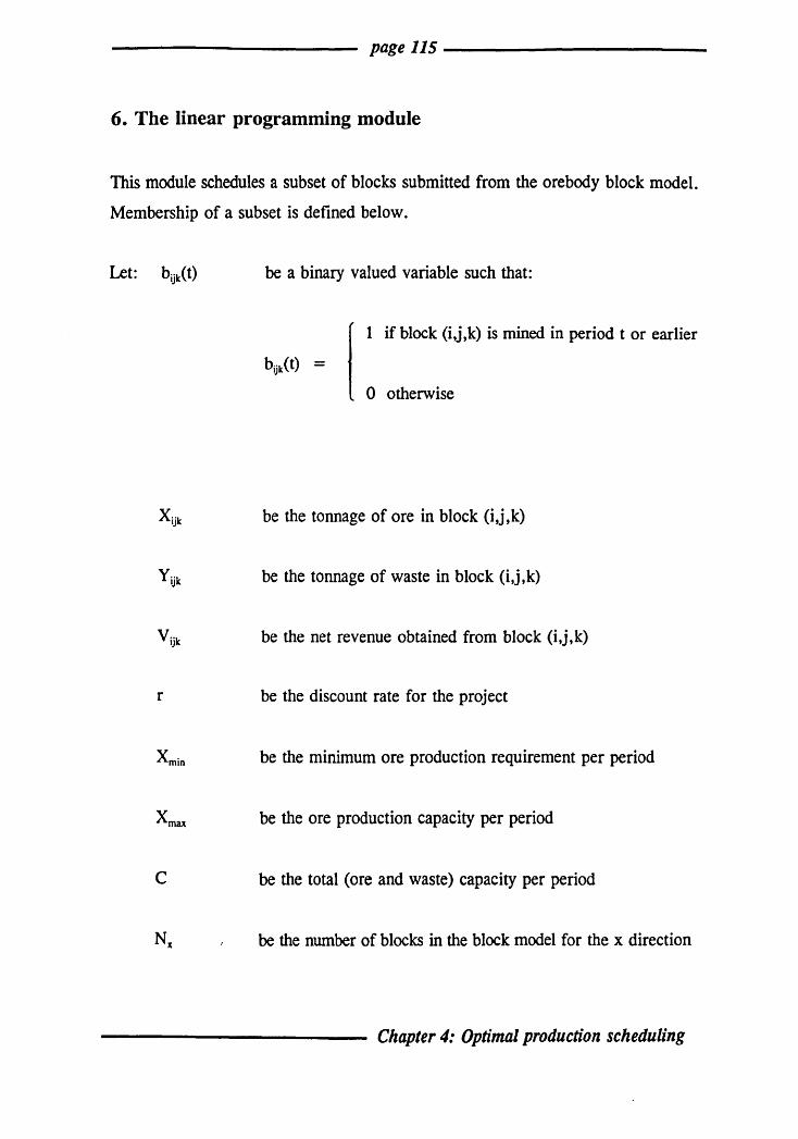
page 115 ------------
6. The linear programming module
This module schedules a subset of blocks submitted from the orebody block model.
Membership of a subset is dermed below.
be a binary valued variable such that:
[
1 if block (i,j ,k) is mined in period t or earlier
bijk(t) = o otherwise
Xijk be the tonnage of ore in block (i,j,k)
Yijk be the tonnage of waste in block (i,j,k)
Vijk be the net revenue obtained from block (i,j,k)
r be the discount rate for the project
Xmin be the minimum ore production requirement per period
Xmax be the ore production capacity per period
C be the total (ore and waste) capacity per period
N 1 be the number of blocks in the block model for the x direction
Chapter 4: Optimal production scheduling

Nz{l)
I
page 116-----------------------
be the number of blocks in the block model for the y direction
be the number of blocks in the block model for the z direction
be the mininmum and maximum vertical interval (number of
levels) of blocks currently considered
be the number of time periods considered for scheduling
The linear program is:
~~~tt Maximize: L.J L L.J bij k{t) ~j k (1 + r)-I ;=1 j=1 k=Nz(l) 1=1
subject to: I'
E btj k-l(t) - btj k(t/) ~ 0 (1)
1=1
t'
E {bi _Ij k(t} + btj-1 k(t} + bij•1 k(t) + bl +1j k(t}} - btj k(t/} ~ 0 (2) 1 =1
with, for (I) and (2): i = 1, Nx j = 1, Ny k = Nz(I}, Nz(2)
t' = 1, tp
for t = 1, tp
N% N Nz(2)
E t E blj it) (X;j k + 1';j k) ~ C ;=1 j=1 k=N,(I)
for t = 1, tp
Chapter 4: Optimal production scheduling

page 117-----------------------
The access constraints for block (i,j ,k) in period t are that the block
immediately above it (constraint 1) and at least one contiguous block on the same
level (constraint 2) must have been mined prior to t or be mined in t. The constraints
for any block which already satisfies these conditions is removed from the linear
program. This results in a significant reduction in the number of access constraints
from that required in the general optimal open pit formulation.
The current formulation is limited to a horizontal array of 2500 (e.g., 50 x
50) blocks, a maximum of three levels open in anyone time period and an upper
limit of three time periods in any linear program. These limitations generate a
maximum of 22,500 variables, 22,500 type (1) access constraints (each containing
a maximum of 4 variables), 22,500 type (2) access constraints (each containing a
maximum of 13 variables) and 10 production capacity constraints. The number of
constraints can (and generally must) be reduced significantly by eliminating those for
blocks that are already accessible, by using the stripping module to make more
blocks accessible and, once mining has begun, by limiting the lateral and horizontal
distances between production areas within and between production periods. This
reduction in the number of constraints is an essential step in the operation of the
program. If the linear program is too large to be solved the user is invited to reduce
the number of constraints, via the waste stripping and mining simulation modules,
by undertaking additional stripping and/or reducing the extent of working areas. If
the lateral extent of working areas is reduced the block indices (N x and Ny) in the
linear program must be adjusted.
Chapter 4: Optimal production scheduling
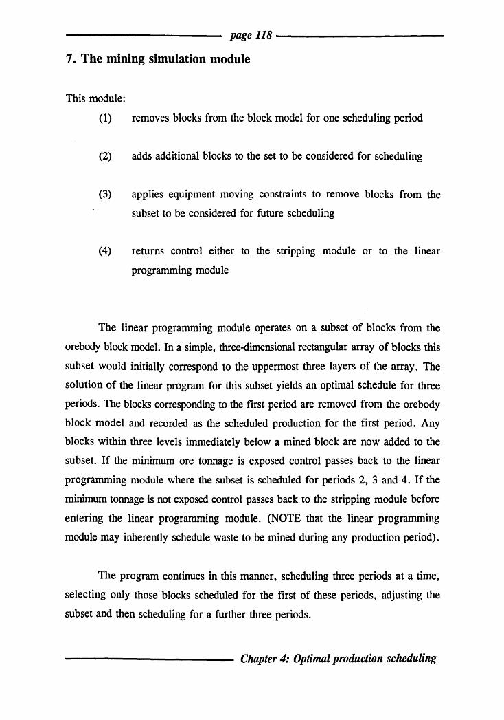
page 118 ------------
7. The mining simulation module
This module:
(1) removes blocks from the block model for one scheduling period
(2) adds additional blocks to the set to be considered for scheduling
(3) applies equipment moving constraints to remove blocks from the
subset to be considered for future scheduling
(4) returns control either to the stripping module or to the linear
programming module
The linear programming module operates on a subset of blocks from the
orebody block model. In a simple, three-dimensional rectangular array of blocks this
subset would initially correspond to the uppermost three layers of the array. The
solution of the linear program for this subset yields an optimal schedule for three
periods. The blocks corresponding to the first period are removed from the orebody
block model and recorded as the scheduled production for the first period. Any
blocks within three levels immediately below a mined block are now added to the
subset. If the minimum ore tonnage is exposed control passes back to the linear
programming module where the subset is scheduled for periods 2, 3 and 4. If the
minimum tonnage is not exposed control passes back to the stripping module before
entering the linear programming module. (NOTE that the linear programming
module may inherently schedule waste to be mined during any production period).
The program continues in this manner, scheduling three periods at a time,
selecting only those blocks scheduled for the first of these periods, adjusting the
subset and then scheduling for a further three periods.
Chapter 4: Optimal production scheduling
page 119 ------------
Once the very frrst production period is scheduled an additional constraint is
imposed on membership of the subset of blocks offered to the linear programming
module. Blocks can only enter the subset if they are within user-specified horizontal
and vertical distances from the blocks scheduled in previous periods. This condition
is critical in reducing the numbers of variables and constraints in the linear program
to yield a formulation that can be solved.
8. Solving the linear program
The major problem in this formulation is in obtaining a solution to the linear
program. Although the formulation is in fact an integer program the nature of the
access constraints is such that they form a unimodular matrix. The capacity
constraints can be manipulated so as to conform to the same matrix structure. The
advantage of this is that the program can be solved as a continuous linear program
without recourse to the more computationally demanding integer programming.
If the numbers of variables and/or constraints in the linear program are too
large control is returned to the mining simulation module where the user is invited
to reduce the horizontal and vertical distance requirements for membership of the
subset of blocks.
It is also possible to use approximate methods of solution such as that
reported in Dowd (1989). At present, however, the software requires a workstation
for implementation. Future developments will focus on the possibility of using
various forms of decomposition to speed up the solution and to reduce storage
requirements.
------------ Chapter 4: Optimal production scheduling

page 120 ------------
8.1 Additional constraints
It is possible to include additional operational constraints. For example, it may be
desirable for blending or similar purposes to maintain the average grade of
production in each time period between upper and lower limits:
where
for t=l, .. ,tp
for t=l, .. ,tp
G I and Gu are the lower and upper limits on grade values
(these may also be specified as functions of time or
geographical locations)
gijk is the grade value of block (i,j,k).
The inclusion of such additional constraints will however substantially
increase computing requirements.
9. Conclusion
The formulation of the scheduling problem given here allows the determination of
an optimal mine schedule using the criterion of maximum net present value. It is
believed that the algorithms used yield a true practical optimum or a solution which
is very close to the true optimum. At present· the algorithm described is limited to
a workstation implementation but it is believed that the use of decomposition
Chapter 4: Optimal production scheduling

page 121 -----------
methods and approximate solution algorithms for the linear programming component
will ultimately yield a PC version.
------------ Chapter 4: Optimal production scheduling
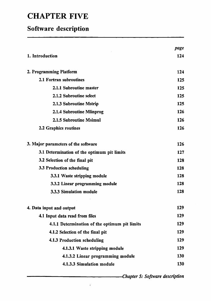
CHAPTER FIVE
Software description
1. Introduction
2. Programming Platform
2.1 Fortran subroutines
2.1.1 Subroutine master
2.1.2 Subroutine select
2.1.3 Subroutine Mstrip
2.1.4 Subroutine Mlinprog
2.1.5 Subroutine Msimul
2.2 Graphics routines
3. Major parameters of the software
3.1 Determination of the optimum pit limits
3.2 Selection of the final pit
3.3 Production scheduling
3.3.1 Waste stripping module
3.3.2 Linear programming module
3.3.3 Simulation module
4. Data input and output
4.1 Input data read from files
4.1.1 Determination of the optimum pit limits
4.1.2 Selection of the final pit
4.1.3 Production scheduling
4.1.3.1 Waste stripping module
4.1.3.2 Linear programming module
4.1.3.3 Simulation module
page
124
124
125
125
125
125
126
126
126
126
127
128
128
128
128
128
129
129
129
129
129
129
130
130
-----------------lChapter 5: Software description

-----------page 123 ------------
4.1.4 Graphics routines
4.2 Output results written to files
4.2.1 Determination of the optimum pit limits
4.2.2 Selection of the final pit
4.2.3 Production scheduling
4.2.3.1 Waste stripping module
4.2.3.2 Linear programming module
4.2.3.3 Simulation module
4.2.4 Graphics routines
5. Software execution
5.1 Determination of the optimum pit limits
5.2 Selection of the final pit
5.3 Production scheduling
5.3.1 Waste stripping module
5.3.2 Linear programming module
5.3.3 Simulation module
5.4 Graphics display of the results
130
130
130
130
131
131
131
131
131
132
132
133
133
134
134
135
136
-----------------lChapter 5: Software description
-----------page 124------------
1. Introduction
The methods described in the previous Chapters have been coded into a set of . programs that have been tested on trial data and on a real data set from a gold
deposit This Chapter describes the main programs in the software package, presents
the different types of data input and output, the major paramters and describes the
execution of the software.
The programs developed during this research project are:
Optimal open pit design by parameterization
Final pit selection
Mine scheduling
Graphics display of the results
All programs are contained in an integrated computer package. The package
is described, section by section, in this Chapter.
2. Programming platform
The software consists of a main program, four main FORTRAN subroutines, and
five UNlRAS routines. The problem is solved entirely in core.
The main program calls the major executable subroutines and graphics routines.
-----------------cChapter 5: Software description

-----------page 125------------
2.1 Fortran subroutines
The following are the main Fortran subroutines of the software:
2.1.1 Subroutine master
This subroutine fmds the optimal open pit limits using the parameterization technique.
The result is a set of technically optimum nested pits, one of which will be the
economic optimum for a given set of economic parameters.
The parameterization technique can produce a set of nested pit designs for
a grade block model (characteristics and plans), in about 30 seconds, or less, of
computer run time on a Sun workstation.
2.1.2 Subroutine select
The determination of optimal ultimate pit limits requires the transformation of the
block grade matrix into a revenue block matrix which can be optimised (scheduled).
Block profit comes from the evaluation of a function of many variables
such as grade of ore, mining costs, transportation costs, price of mineral, etc. The net
value for each block is the actual cost or profit realised by mining and processing that
block. Blocks with positive profit have a final value which exceeds the total of all
costs (mining, production, transport, etc.) whereas negative profit blocks do not.
2.1.3 Subroutine Mstrip
The subroutine strips waste blocks so as to expose the minimum ore tonnage at the
start of each mining period. The minimum ore tonnage is specified by the user and
is determined by the program in terms of numbers of accessible ore blocks.
------------------(Chapter 5: Software description
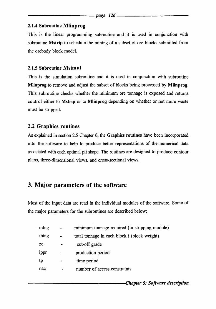
----------------------page 126---------------------
2.1.4 Subroutine Mlinprog
This is the linear programming subroutine and it is used in conjunction with
subroutine Mstrip to schedule the mining of a subset of ore blocks submitted from
the orebody block model.
2.1.5 Subroutine Msimul
This is the simulation subroutine and it is used in conjunction with subroutine
Mlinprog to remove and adjust the subset of blocks being processed by Mlinprog.
This subroutine checks whether the minimum ore tonnage is exposed and returns
control either to Mstrip or to Mlinprog depending on whether or not more waste
must be stripped.
2.2 Graphics routines
As explained in section 2.5 Chapter 6, the Graphics routines have been incorporated
into the software to help to produce better representations of the numerical data
associated with each optimal pit shape. The routines are designed to produce contour
plans, three-dimensional views, and cross-sectional views.
3. Major parameters of the software
Most of the input data are read in the individual modules of the software. Some of
the major parameters for the subroutines are described below:
. mtng
ibtng
zc
ippr
tp
nac
minimum tonnage required (in stripping module)
total tonnage in each block i (block weight)
cut-off grade
production period
time period
number of access constraints
------------------------cChapter 5: Software description
----------------------page 127------------------------
ncc
mco
mcw
mpc
pog
rd
number of capacity constraints
mining cost of ore
mining cost of waste
processing cost
price of gold
discount rate for the project
irs, jsr, mrs, nrs, isr, jsr - right-hand-side values for the different constraints.
ile, ieq, ige . - types of constraints, less than or equal to, equal to, and greater
than or equal to.
Some parameters are calculated, e.g.
itbc
itnc
nbp
number of blocks in the subset
total number of constraints to be considered
number of blocks to be mined per period
Parameters not mentioned above are better explained as appropriate in the
following sections of this Chapter.
3.1 Determination of the optimum pit limits
The parameters introduced interactively by the user when running this section of the
software are:
zc
x, y, z
bw
alpha
cut-off grade
block dimensions
specific gravity of ore
the final pit slope (degrees)
-------------------------cChapter 5: Software description
----------------------page 128-----------------------
3.2 Selection of the final pit
The selection of the final pit plan requires the specification of the following
parameters:
Price of the metal
Mining costs
Processing costs
3.3 Production scheduling
As explained in the previous sections the scheduling section is run in three stages
where the data are entered via the keyboard or read from files and are passed
between routines by means of COMMON blocks or as arguments of subroutines. The
following sections list the parameters that are entered via the keyboard by the user
in response to requests that appear on the screen for that part of the schedule.
3.3.1 Waste stripping module
The following parameters are required for this section:
itnb total number of variables in the optimum pit plan.
nnb number of blocks to be exposed (as minimum ore tonnage).
3.3.2 Linear programming module
All parameters required by this section (right-hand-side, the rowtype (+/-) for
different types of constraints) are entered by means of COMMON blocks or as
arguments.
The direction of optimization is entered as: + for maximization and
- for minimization (not used)
3.3.3 Simulation module
Block coordinates of the selected ore blocks are the major input parameters for this
section.
---------------------cChapter 5: Software description
-----------page 129------------
4. Data input and output
To execute the software two types of data are required. The first type of data are
those supplied from files, COMMON blocks and as parameters; these are explained
in this section The second type are those entered interactively and these are described
in the software execution section.
4.1 Input data read from files
The software is a set of programs set up for the design of the optimum open pit
shape and production scheduling. Therefore, most of the data files are common to
nearly all the sections of the software. The following are the input data files required
for each section of the software, all of them being in comma-delimited free format.
4.1.1 Determination of the optimum pit limits
Beside the interactive input data, the grade file is the major input file for this section
of the software.
4.1.2 Selection of the final pit
The grade file mentioned above is used again in this section to produce an equivalent
three-dimensional revenue block model file.
4.1.3 Production scheduling
These are three sections in the model which work together.
4.1.3.1 Waste stripping module'
The grade file is the input for this section, together with a corresponding three
dimensional file, recording the removed blocks.
-----------------cChapter 5: Software description
----------------------page 130------------------------
4.1.3.2 Linear programming module
A subset of blocks, selected by the user, in the fonn of a data file is submitted to this
section. A simplex matrix for solution of LP module is produced. The matrix
includes the equation of the objective function and the integer declaration of the
variables being considered.
4.1.3.3 Simulation module
A data file created in the previous section, is submitted to this section as an input
data file. The file contains the blocks to be removed in each time period.
4.1.4 Graphics routines
The grade file and the optimum pit plan are the main data input files for this section.
Both files are used to produce different graphics representations of the characteristics
of the optimum pit.
4.2 Output results written to files
Each section of the software generates its own output files with the file names set up
in the software. Each relevant output is described in the following sections.
4.2.1 Determination of the optimum pit limits
Output from this section is in two forms. The fITst is a binary file created for efficient
storage and data transfer when used by other programs (not discussed here). The
second is an ASCII file containing full details of the characteristics of each individual
pit. Plans of the nested pits are given as grade distributions or depth levels, and both
can be contoured.
4.2.2 Selection of the final pit
The output from this section comprises pit by pit revenue values together with the
pit with the maximum revenue value.
------------------------------«Chapter 5: Software description

----------------------page 131------------------------
4.2.3 Production scheduling
The output files of blocks being selected and removed from the orebody block model
during the scheduling process are produced in each individual section of this part of
the software.
4.2.3.1 Waste stripping module
The output of this section is a table showing the appropriate priority given to each
block together with the pit plans showing the blocks removed during the operation
of the module.
4.2.3.2 Linear programming module
The output from this section is a period by period summary of mined blocks and
final objective function value.
4.2.3.3 Simulation module
The outputs of this section are pit plans of each production period showing the
coding of the removed blocks during the stripping and linear progamming modules.
4.2.4 Graphics routines
This section produces different graphic representations (cf. section 2.5 Chapter 6) of
the optimum pit.
----------------cChapter 5: Software description

-----------page 132 ------------
5. Software execution
The software is executed by running the exec file rebh2.exe created by the UNILINK
system after frrst setting up the UNlRAS environment. The execution starts with the
pit limit determination, followed by pit sequencing and ends with the graphics display
of the results. The software requires two types of data :
The first set is read from files and has been discussed above. The second set
is entered interactively during the software execution and includes all data that are
affected daily, monthly or yearly by market conditions. The reading of the data
depends on the order of the sections where the order is pit limit determination,
scheduling and finally graphics representations.
5.1 Determination of the optimum pit limits
This is the frrst section to be executed and focuses mainly on the pit design. It starts
with the pit limits determination followed by pit selection (the pit with the highest
profit).
Note : There are three options for the output files at the end of the first part
of the determination of the optimum pit limit. Option (2) is set for the software
which contains the pit plans (nested pits) produced during the running of that part of
the software to be optimized. The other two options (1,3) terminate the process. The
rest of the software is described below:
Type in the exec file name: rebh2.exe
Execution starts:
'Operating in the pit design module'
----------------cChapter 5: Software description
-----------page 133------------
Enter the cut-off grade
>
Enter block dimensions (x,y,z directions) and density
>
Enter the final pit slope (degrees)
>
Solution reached: there are 'n' number of pits.
Do you want a full output listing (1);
a pit by pit plan (2);
or just a pit parameter summary (3).
When option (2) is selected the process will continue as follows.
5.2 Selection of the final pit
Parameters required for the pit selection are passed through common blocks.
- Price of the metal
- Mining costs
- Processing costs
Once the final pit is selected, which is automatic, programme control passes to the
following section (Production scheduling).
5.3 Production scheduling
This section has three parts: Waste stripping module, Linear Programming module
and the Simulation module.
This part starts by:
----------------cChapter 5: Software description
-----------page 134------------
Enter subset dimensions (i, j and k)
>
Checks if the coordinates are within the feasible zone of X, Y, Z?
No - Print' NB of ELEM. should not be exceeded, try again'
Yes - The process will continue in the next section (stripping).
5.3.1 Waste stripping module
The module requires the following parameter :
Enter the number (nnb) of blocks per period
>
Checks if the nnb of blocks is greater than the total nb of blocks ?
Yes - Print ' NB of ELEM. should not be exceeded, try again'
No - The process will be resumed as follows:
Exposes the nnb blocks
Checks if the minimum ore tonnage is exposed ?
Yes - Formulate the subset of blocks then continue to the following section
(linear programming).
No - Do you want to increase the number of blocks ?
Yes - Enter the nnb of blocks and control returns to the stripping module
No - Ends the run.
5.3.2 Linear programming module
F or this part of the scheduling moSt of the data are entered in the main program and
are passed to the LP module through CALLs and COMMON blocks.
Program starts:
-----------------cChapter 5: Software description

-----------page 135------------
Enter direction of optimization :
> + (plus) for maximization (used in the current example) or
> - (minus) for minimization (not used in this formulation)
Formulate the LP input
Optimization operation takes place
Is there any solution ?
Yes - Results are put into table format and the control is returned to the next
section (simulation).
No - Means more stripping needed, control is returned to the above section
( stripping module).
5.3.3 Simulation module
The co-ordinates of the selected ore blocks are required here.
Removes blocks of the first time period of the current production period.
Adjusts the subset of blocks
Checks if the minimum ore tonnage is exposed ?
Yes - Control is returned to the above section (linear programming module).
No - Control is returned to the above section (waste stripping module).
Note : The blocks selected and removed from the matrix in each period are
assigned the current production period number.
----------------IChapter 5: Software description

-----------page 136------------
5.4 Graphics display of the results
This section will display graphically some of the characteristics of the optimum pit
plan.
Do you want a graphics display yes/no ?
> Yes - The process will continue as below
> No - Ends the run
Do you want the graphics display to be ?
Enter 1. Pitselection
Enter 2. Optpitj)lan
Enter 3. Optpit_3d_ view
Enter 4. Optpit_x_section
Enter 5. Optpit_inv _section
> Enter the choice
Do you want the display to be ?
Enter 1. For the screen
Enter 2. For HPGL
Ente r 3. For BIW PS
Enter 4. For colour PS
Enter O. To quit
> Enter the choice
Please wait for the graph.
----------------cChapter 5: Software description

-----------page 137------------
To quit the graphics environment press return while the arrow of the cursor
is on the graphics window Thank you.
---------------..(Chapter 5: Software description

CHAPTER SIX
Case study
page
1. Introduction 139
2. Algorithms and their logic 140
2.1 The data requirements 140
2.2 Determination of the optimum pit limits 143
2.3 Selection of the final pit 144
2.4 Production scheduling 145
2.4.1 Waste stripping module 149
2.4.2 Linear programming module 154
2.4.3 Simulation module 160
2.5 Graphics representations 172
2.5.1 Selection of the fmal pit 174
2.5.2 Two-dimensional contouring of mining levels 175
2.5.3 Three-dimensional representation of the optimum
pit plan 176
2.5.4 Cross-sectional views of pit elevations 177
2.5.5 Display of pit that has been mined 178
2.6 The validation of the methodology 179
3. Conclusion 179
------------------ Chapter 6: Case study
-----------page 139------------
1. Introduction
"Optimal open pit design is essentially a computer based implementation of an
algorithm which is applied to a three-dimensional block model of an orebody. Almost
all optimal open pit design algorithms, with the exception of elementary methods
applied to some stratiform deposits, are applied to a regular, fixed, three-dimensional
block model of an orebody. The orebody is subdivided into regular blocks and a
value is estimated for each block. This value is almost always the net (undiscounted)
revenue that would be obtained by mining and treating the block and selling its
contents. Some methods, such as parameterization, use grade values in the block
model. Stuart (1992) proposes an irregular three-dimensional model in which the
orebody is represented by a series of arbitrary geometrical solids. Whilst such a
model is a useful way of representing highly irregular and complex-shaped stratiform
deposits it is doubtful whether sophisticated computer algorithms are really necessary
for the design of optimal pits in such cases." (Dowd, 1994b). The block model is the
fundamental input to the pit design and the scheduling programs developed during
this research project.
The blocks to be mined in each mining period are selected, within the limits
of the given economic constraints, so as to maximize the Net Present Value (NPV)
for the life of the mine.
In general, the production scheduling procedures determine which blocks of ore
and waste should be removed in each mining period so as to maximize the Net
Present Value for the mine, subject to the mining and milling operating constraints.
The scheduling problem is treated in three modules (the modules are documented in
Chapter 4). This Chapter describes the software and presents the results obtained
from applying it to some of the data sets.
------------------- Chapter 6: Case study
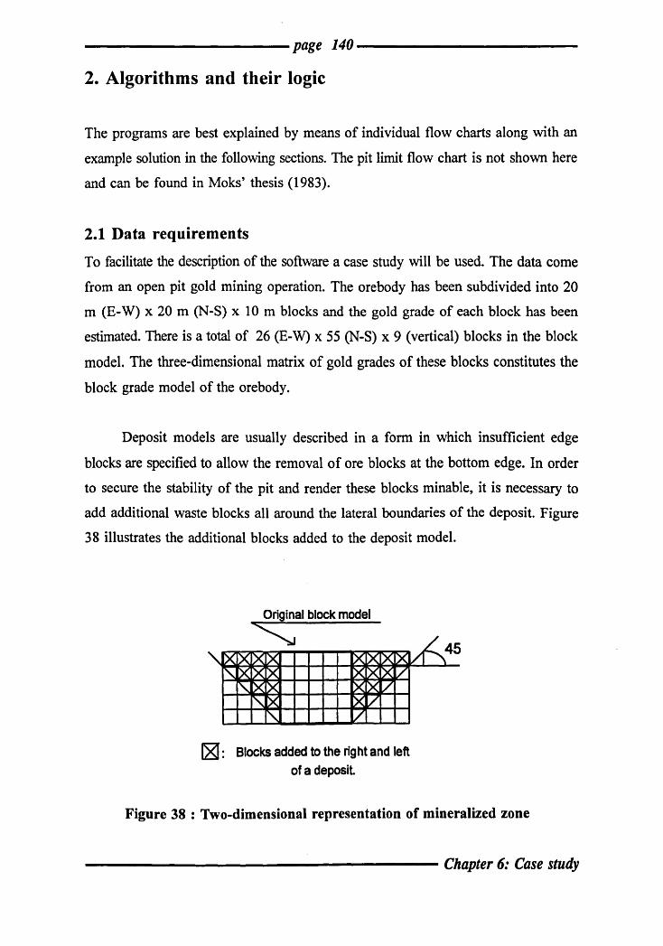
----------------------page 140-----------------------
2. Algorithms and their logic
The programs are best explained by means of individual flow charts along with an
example solution in the following sections. The pit limit flow chart is not shown here
and can be found in Moks' thesis (1983).
2.1 Data requirements
To facilitate the description of the software a case study will be used. The data come
from an open pit gold mining operation. The orebody has been subdivided into 20
m (E-W) x 20 m (N-S) x 10m blocks and the gold grade of each block has been
estimated. There is a total of 26 (E-W) x 55 (N-S) x 9 (vertical) blocks in the block
model. The three-dimensional matrix of gold grades of these blocks constitutes the
block grade model of the orebody.
Deposit models are usually described in a form in which insufficient edge
blocks are specified to allow the removal of ore blocks at the bottom edge. In order
to secure the stability of the pit and render these blocks minable, it is necessary to
add additional waste blocks all around the lateral boundaries of the deposit. Figure
38 illustrates the additional blocks added to the deposit model.
Original block model
"':J ~~ ~ x )( )()()(X
:'\. X X)( x )( x / ~ ~f)( ~ )c: /
,>< >< k( , /
~ : Blocks added to the right and left ofa deposit
~45
Figure 38 : Two-dimensional representation of mineralized zone
------------------ Chapter 6: Case study
----------------------page 141-----------------------
Because of the similarity of all the deposit areas the number of blocks added
is equal in all four cardinal directions and is determined as the number of levels of
the deposit. The number of blocks added to the orebody block model on the northern
and southern boundaries as well as on the eastern and western boundaries, must
satisfy the lowest slope angle of any area of the deposit.
The initial data required are :
1. the cut-off grade
2. the block dimensions (rows, columns, levels, directions)
3. the specific gravity of ore and waste
4. the final pit slope
5. the grade of each block
The scheduling algorithm requires the block grade model to be transformed
into a revenue block model which can be used by the optimization module (LP). The
data and block revenue calculations required are described in the following
paragraphs.
For the sake of a simple example, a horizontal subset plane of 100 (i.e., 10
x 10) blocks, a maximum of three levels open in any time period, and an upper limit
of three time periods in any linear program has been selected from the total ore body
block grade model. The subset will be used to show the input data for solving the
schedule problem in the following sections.
Each row of the three-dimensional array of data contains the x, y, and z co
ordinates of the mid-point of a block, together with the average grade and the
tonnage above the cut-off grade in that block.
The data used in this example are:
cut-off grade 0.2 glt
---------------------- Chapter 6: Case study

-----------page 142 ------------
specific gravity
ore mining costs
waste mining costs
processing costs
price of gold
2.74 tlm3 for both ore and waste
£ 3.00/tonne
£ 1.50 / tonne
£ 4.50 / tonne
£ 9,500/ kg
The total tonnage of each block is: 20 x 20 x 10 x 2.74 = 10960 tonnes
The tonnes of waste in each block can be calculated as:
10960 - ore tonnage in block.
To illustrate the revenue calculations consider the following record extracted
from the data file :
1500.00 750.00 55.00 3.25 3200
i.e. block is centred on co-ordinates (1500, 750, 55) and contains 3200 tonnes of ore
above cut-off grade at an average grade of 3.25 g/t. The revenue value of this
particular block is:
Amount of waste = 10960 - 3200 = 7760 tonnes
Cost of mining waste = 7760 x 1.50 = £11640
Cost of mining ore = 3200 x 3.00 = £9600
Processing cost = 3200 x 4.50 = £14400
Value of contained gold = 3200 x 3.25/1000 x 9500
= £98800
Net revenue = 98800 - 11640 - 9600 - 14400
= £63160
Blocks with missing or unestimated grades and tonnages are recorded as -999.0
in the data file and are regarded as waste for the purpose of calculating revenue
------------------- Chapter 6: Case study

----------------------page 143-----------------------
values, i.e. they are treated as 10960 tonnes at 0.0 g/t. (most of these data are around
the edges and can be deleted from the file to reduce the number of blocks).
In order to show the applicability of the methodology used in the current study,
two example solutions are summarized in the following sections.
Some information and the results of planning with three production periods are
shown in the tables and figures throughout the following sub-sections of this Chapter.
Two matrices are used during the process: one representing the states of the blocks
(mined or not mined) as shown in figure 44 where the removed blocks are
represented by 1, while the remaining blocks are represented by O. The other matrix
represents the fmal coding of the removed blocks as shown in figure 45 where, 1,2,3
represent the sequential removal of blocks during the three different production
periods. In both matrices, the blocks outside the optimum pit plan are represented by
N3 + I (Le. the number of levels plus one in the program), i.e. lOin this particular
example.
2.2 Determination of the optimum pit limits
The optimum pit limits are found using the parameterization technique. The following
parameters are required : cut-off grade, slope angle and the planning parameters. The
application of an algorithm to the block grade model yields a set of technically
optimum nested pits, one of which will be the economic optimum for a given set of
economic parameters.
The parameterization technique can produce a set of nested pits from a block
grade model comprising 100,000 blocks in approximately 30 seconds of CPU time
on a Sun workstation. The results are stored in a number of files to be used by other
programs. The file used in the following sections contains a two-dimensional plan of
numbers representing the levels and shows the number of blocks to be mined in each
vertical column to obtain the maximum profit. The two-dimensional representation
of the optimum pit plan is shown in figure 39.
------------------------ Chapter 6: Case study

------------page 144------------
2.3 Selection of the final pit
A pit plan file containing the total number of pit plans generated in the previous
section is used to determine the pit with the highest profit. This pit determination
requires the transformation of the block grade matrix into a revenue file matrix which
can be scheduled.
The simple revenue formula described in Chapter 2, as well as in the numerical
example in section 2.1 of this Chapter, is used to determine the pit with the highest
profit as shown in table 1. The data required are the price of the metal, the mining
costs and the processing costs.
pit number *********
1 2 3 4 5 6 7 8 9
10 11 12 13 14 15 16 17 18 19
value ***** -1.644 29.820 30.464 39.868 69.431
105.049 628.203 746.419 793.935 949.353
1035.996 1590.774 1743.745 2400.809 2431.968 2623.167 2780.683 3007.691 3072.965
the maximum pit(i) and its value are :
19 3072.965
Table 1 : Pit plans evaluation
------------------- Chapter 6: Case study
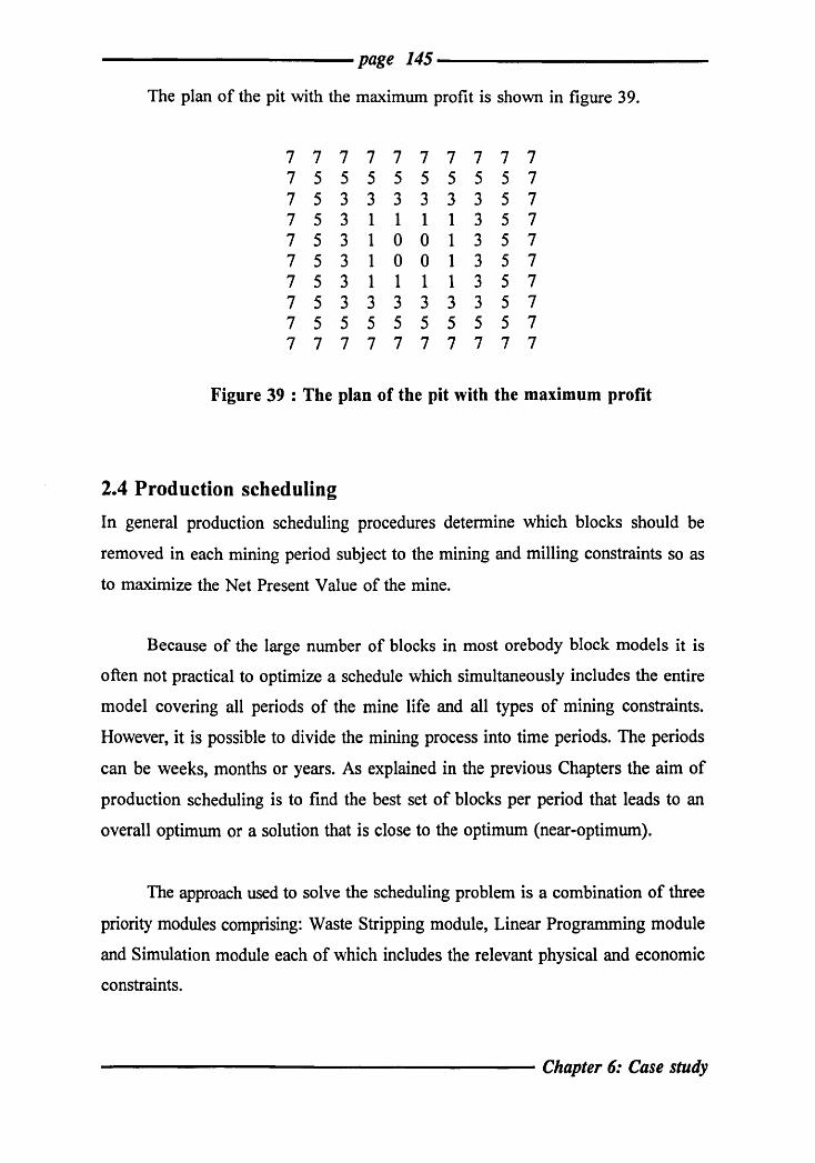
page 145
The plan of the pit with the maximum profit is shown in figure 39.
7 7 7 7 7 7 7 7 7 7 7 5 5 5 5 5 5 5 5 7 7 5 3 3 3 3 3 3 5 7 7 5 3 1 1 1 1 3 5 7 7 5 3 1 0 0 1 3 5 7 7 5 3 1 0 0 1 3 5 7 7 5 3 1 1 1 1 3 5 7 7 5 3 3 3 3 3 3 5 7 7 5 5 5 5 5 5 5 5 7 7 7 7 7 7 7 7 7 7 7
Figure 39 : The plan of the pit with the maximum profit
2.4 Production scheduling
In general production scheduling procedures determine which blocks should be
removed in each mining period subj ect to the mining and milling constraints so as
to maximize the Net Present Value of the mine.
Because of the large number of blocks in most orebody block models it is
often not practical to optimize a schedule which simultaneously includes the entire
model covering all periods of the mine life and all types of mining constraints.
However, it is possible to divide the mining process into time periods. The periods
can be weeks, months or years. As explained in the previous Chapters the aim of
production scheduling is to find the best set of blocks per period that leads to an
overall optimum or a solution that is close to the optimum (near-optimum).
The approach used to solve the scheduling problem is a combination of three
priority modules comprising: Waste Stripping module, Linear Programming module
and Simulation module each of which includes the relevant physical and economic
constraints.
------------------- Chapter 6: Case study

------------page 146-------------
The following parameters were specified for this example:
250,000 t/year minimum ore production requirement
500,000 t/year maximum ore production capacity
1,000,000 t/year total (ore + waste) capacity
Discount rate 10 %.
The above parameters are subject to change. The capacity values must be
varied proportionally with the number of blocks in the subset treated in more than
one time period. This is to avoid false violation of capacity constraints (see also
section 6 in Chapter 4).
A brief illustration of the algorithms is provided in the flow chart in figure 40.
A more comprehensive explanation with results is provided in subsequent sections.
The modules are set to run for three production periods (ippr), and a limit of
three time periods (tp) in any linear program. The determination of an optimal mine
schedule using the criterion of maximum Net Present Value is the target for each
production period.
To start the scheduling part of the software a subset of blocks to be optimized
is specified fITst. The co-ordinates of the subset should be within the co-ordinates x,
y and z of the optimum pit limits. The total number of blocks (itbc) of the subset to
be optimised, the possible total number (itnc) of constraints involved and the number
of blocks (nbp) to be mined per time period are calculated.
On calculation of these parameters the program proceeds by calling the
stripping module (STRIP) to expose a minimum ore tonnage (MOT) before the start
of any production period. The minimum ore tonnage is a set of blocks specified by
the user and determined by the module as accessible ore blocks to be exposed before
production starts.
------------------- Chapter 6: Case study

------------page 147------------
If this condition is not satisfied the process is repeated until the condition is
satisfied. The waste stripping module proceeds by formulating the subset of blocks
to be used in the next module (LP).
The subset of blocks is then transformed into table format and optimized by
the LP module. If there is no solution to the subset of blocks within the LP module,
control is returned to the waste stripping module where more stripping takes place.
However, if there is a solution then the blocks (BK) selected to be removed in each
time period, are put into table format in terms of co-ordinates and control is sent
forward to the simulation module.
The simulation module (SIMUL), then removes the blocks scheduled for the
frrst time period, adjusts and checks the minimum ore tonnage of the new subset of
blocks, then returns the control either to the linear programming module for more
planning or to the waste stripping module for more stripping.
The process is repeated by iteration between the three modules for the total
number of production periods. Intermediate results for the different sections of the
scheduling part of the software can be obtained for each iteration.
------------------- Chapter 6: Case study

-----------------------page 148-------------------------
ll'R - 0 IPPR -3
IFLAG -0 X.Y.Z
Figure 40 General structure of the schedule model
------------------- Chapter 6: Case study

----------------------page 149-----------------------
2.4.1 Waste stripping module
The selection of the waste blocks to be mined prior to production is, in general, a
trade-off between minimizing the amount of waste material removed and maximizing
the value of the ore blocks exposed at the end of the pre-production stripping.
This module is used only when required to expose a minimum ore tonnage at
the start of each production period. This would normally be called a pre-production
module and would be used to schedule waste and overburden and provide access to
ore blocks. The main steps of the waste stripping module are summarized in figure
41.
Waste blocks have to be removed at some time, either during the same period
that an ore block is mined or at least one period before, i.e. waste blocks directly
or indirectly overlying ore blocks must be assigned high priority coefficients so that
they will be mined first.
To establish the priority of the various blocks to be exposed as ore blocks, the
grade and the number of exposed sides of blocks are used as constraints (all
constraints are used simultaneously).
To run the module for this example the following data were specified:
1. A minimum ore tonnage to be mined is specified and is translated by the program
into the number of accessible ore blocks.
2. A guess of a total number of blocks at a cut-off of 0.2 g/t, that are likely to sum
up to the minimum ore tonnage specified. The user is then repeatedly prompted to
provide a better estimate if this tonnage is not met by the current number of blocks,
until it is. The current module is able to expose any number of blocks up to the total
number of blocks within the optimum pit plan if necessary.
--------------------------- Chapter 6: Case study
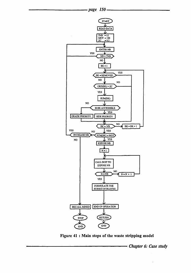
-----------page 150------------
Figure 41 : Main steps of the waste stripping model
------------------- Chapter 6: Case study

----------------------page 151------------------------
In due course, this interactive part of the software can be automated through
a formal iterative numerical scheme. When the requirement is satisfied control is
passed forward to the LP module for further planning. The internals of the current
interactive iterative scheme have as follows :
The selected blocks (BK) are examined one by one. If the grade of a minable
block is greater than or equal to the cut-off grade a priority coefficient is assigned
to that block depending first of all on the number of its sides that are currently
exposed. In a similar way a priority coefficient is assigned to the same block
depending on its grade value.
The procedure continues until the minimum ore tonnage requirement is
satisfied. By then all minable blocks (nnb) should have been examined and assigned
a priority number. The result of such an operation for 20 minable blocks is shown
in table 2.
Selected : Exposed : Grade : Priority of : blocks : sides g/t blocks
-----------------:--------------:------------:------------------: 11 2 0 2.100 9 212 0 2.200 8 312 0 4.900 3 412 0 3.300 7 512 0 7.900 '2 612 0 3.600 6 712 0 1.900 10 812 0 1.900 10
Table 2 : Order of priority of blocks (continued ... )
------------------------ Chapter 6: Case study

------------page 152 ------------
912 1012 122 222 322 422 522 622 722 822 922
1022
o 4.800 o 3.600 o 2.100 o 3.300 o 0.900 o : 16.100 o 1.800 o 3.600 o 3.700 o 3.600 o 1.900 o 3.600
Table 2 ( ••• continued)
4 6 9 7
12 1
11 6 5 6
10 6
In this example the ore blocks are not exposed at the beginning of the first
production period. As can be seen in table 2, the priority classification is mainly
based on the grades of the blocks instead of their exposed sides. Block (4,2,2) with
grade 16.10 g/t, has priority number 1. The priority is given in that order until the
last block with the lowest grade is given the smallest priority number i.e. block
(3,2,2) with a grade 0.90 glt has priority number 12.
The blocks would have been assigned priority numbers in a similar way if
classification had been based on exposed sides. The block with the highest number
of exposed sides would have priority number 1 and so on. It is important to note that
------------------- Chapter 6: Case study
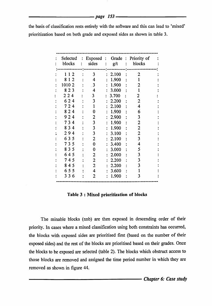
------------page 153 ------------
the basis of classification rests entirely with the software and this can lead to 'mixed'
prioritization based on both grade and exposed sides as shown in table 3.
: Selected : Exposed : Grade : Priority of blocks sides g/t blocks
:----------------:--------------:------------:-------------------: 1 1 2 812
1010 2 823 224 624 724 824 924 734 834 294 635 735 835 645 745 845 655 336
3 4
.3 4 3 3 1 o 2 3 3 3 2 o o 2 2 2 4 2
2.100 1.900 1.900 3.000
: 3.700 2.200 2.100 1.900 2.900 1.900 1.900 3.100 2.100 3.400 3.000 2.000 2.200 2.200 3.600 1.900
2 1 2 1 2 2 4 6 3 2 2 2 3 4 5 3 3 3 1 3
Table 3 : Mixed prioritization of blocks
The minable blocks (nnb) are then exposed in descending order of their
priority. In cases where a mixed classification using both constraints has occurred,
the blocks with exposed sides are prioritised first (based on the number of their
exposed sides) and the rest of the blocks are prioritised based on their grades. Once
the blocks to be exposed are selected (table 2). The blocks which obstruct access to
those blocks are removed and assigned the time period number in which they are
removed as shown in figure 44.
------------------ Chapter 6: Case study
-----------page 154------------
The removal of blocks in this module is based on geometrical constraints. The
geometrical constraints for this module are:
- a block can only be mined if the five blocks above it have already been mined
- the slope angle of 45 degrees must be maintained
Removed blocks are generally blocks of zero or low grades within the
optimum pit plan.
A successful run of the module will expose the ore blocks and, create access
to them and will reduce the number of constraints in the next module (LP). After
exposing the selected ore blocks the module will formulate the subset of blocks to
be used in the next module (LP). In order to minimize movement of equipment, the
blocks added to the subset are the closest blocks to those exposed in the waste
stripping module.
Pre-production stripping usually happens in the first year of operation and it
would be rare for it to be conducted during the productive life of the mine. However,
if it does happen during the time horizon of the scheduling algorithms then the
removed blocks are always considered as part of the current production period.
2.4.2 Linear programming module
The linear programming (LP) module optimizes ore removal of a subset of blocks
from the orebody block model and, as such, it handles the physical and economic
constraints. The Lp_solve source code described in Chapter 3, section 2.2.2 was
incorporated into the author's software, to solve the LP part of the work.
------------------ Chapter 6: Case study
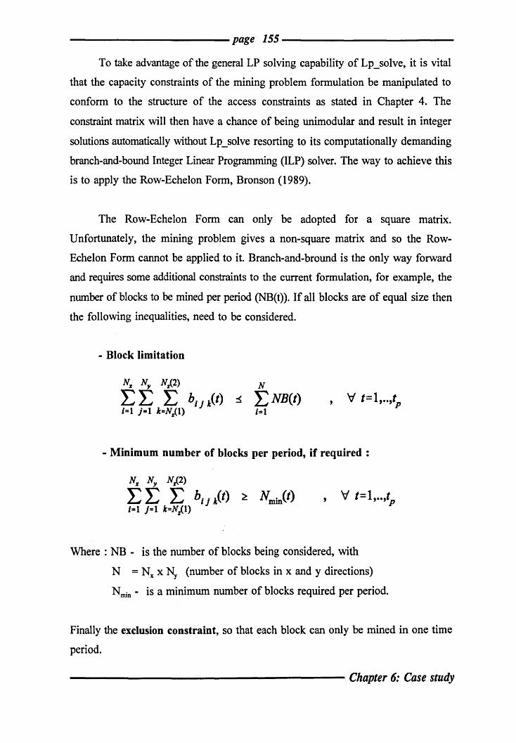
------------page 155-------------
To take advantage of the general LP solving capability of Lp_solve, it is vital
that the capacity constraints of the mining problem formulation be manipulated to
conform to the structure of the access constraints as stated in Chapter 4. The
constraint matrix will then have a chance of being unimodular and result in integer
solutions automatically without Lp _solve resorting to its computationally demanding
branch-and-bound Integer Linear Programming (ILP) solver. The way to achieve this
is to apply the Row-Echelon Form, Bronson (1989).
The Row-Echelon Form can only be adopted for a square matrix.
Unfortunately, the mining problem gives a non-square matrix and so the Row
Echelon Form cannot be applied to it. Branch-and-bround is the only way forward
and requires some additional constraints to the current formulation, for example, the
number of blocks to be mined per period (NB(t». If all blocks are of equal size then
the following inequalities, need to be considered.
- Block limitation
Nz Ny Nz<2) N
E E E bi } k(t) :S ENB(t) i=1 j=1 k=Nz<I) i=1
V t=l, .. ,tp
- Minimum number of blocks per period, if required:
V t=l, .. ,tp
Where : NB - is the number of blocks being considered, with
N = Nx x Ny (number of blocks in x and y directions)
Nrnin - is a minimum number of blocks required per period.
Finally the exclusion constraint, so that each block can only be mined in one time
period.
------------------ Chapter 6: Case study
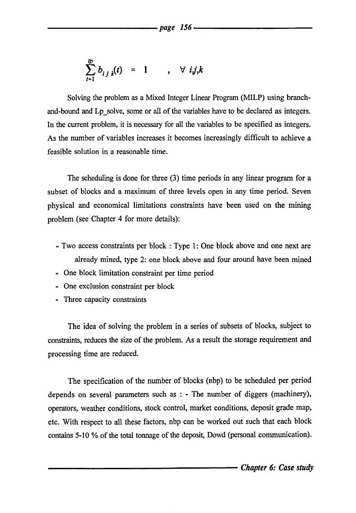
----------------------page 156------------------------
'if ij,k
Solving the problem as a Mixed Integer Linear Program (MILP) using branch
and-bound and Lp _solve, some or all of the variables have to be declared as integers.
In the current problem, it is necessary for all the variables to be specified as integers.
As the number of variables increases it becomes increasingly difficult to achieve a
feasible solution in a reasonable time.
The scheduling is done for three (3) time periods in any linear program for a
subset of blocks and a maximum of three levels open in any time period. Seven
physical and economical limitations constraints have been used on the mining
problem (see Chapter 4 for more details):
- Two access constraints per block : Type 1: One block above and one next are
already mined, type 2: one block above and four around have been mined
- One block limitation constraint per time period
- One exclusion constraint per block
- Three capacity constraints
The idea of solving the problem in a series of subsets of blocks, subject to
constraints, reduces the size of the problem. As a result the storage requirement and
processing time are reduced.
The specification of the number of blocks (nbp) to be scheduled per period
depends on several parameters such as : - The number of diggers (machinery),
operators, weather conditions, stock control, market conditions, deposit grade map,
etc. With respect to all these factors, nbp can be worked out such that each block
contains 5-10 % of the total tonnage of the deposit, Dowd (personal communication).
------------------- Chapter 6: Case study

----------------------page 157------------------------
The nbp for the current study is taken to be the number of blocks on one level (x*y)
of the deposit for each production period.
The main steps of an examination of the subset of blocks in the context of the
LP module are given in figure 42.
The above fonnulation generates a simplex matrix for solution of LP module
as MAT(169 ; 324) i.e. 169 constraints and 324 variables using the waste stripping
module. The matrix includes the elements of the constraint matrix, the equation of
the objective function and the integer declaration of the variables being considered.
The computer processing for the above subset of blocks was completed for three
production periods.
The elements of the constraint matrix generated depend on the accessibility of
blocks. If a block is accessible then the accessibility constraints for that particular
block are eliminated from the matrix. A block is accessible if the block above it and
at least one of the blocks surrounding it on the same level have already been
removed. However, if a block is on the uppennost level (level one) then it is always
accessible because the blocks above it are air blocks. The module considers all air
blocks are removed first.
The module can indicate whether or not there is a solution. In either case
control is always returned to the scheduling algorithm where decisions can be made.
No solution to the MILP problem may be caused by too large a number of
blocks, by one of the constraints not being satisfied. In order to continue the
planning process more ore blocks must be exposed. In such cases control is returned
to the waste stripping module where more waste blocks are stripped to expose more
ore blocks.
-------------------------- Chapter 6: Case study

----------------------page 158------------------------
Figure 42 Main steps of the linear programming module
---------------------- Chapter 6: Case study

-----------page 159------------
However, in the example quoted here an optimum solution exists. The LP
module generated an optimal solution for the three time periods used. The results
were the values of the X decision variables which represent the status of the blocks
to be mined from any specific subset of blocks and the profit that can be gained
from that subset of blocks during the three time periods.
The X decision variables are converted into their corresponding block co
ordinates (i,j,k). Due to the exclusion constraint, each block of the subset can only
be mined in one time period. The method of mining is by push-back. The starting
block is always the last block to be mined. As can be seen in table 4, the block with
co-ordinates i=3, j=9, k=3, is considered first in the LP solution, where as it is in
fact the last block to be mined.
Scheduling Production Period : 1
LinProg Periods 3
No of Removed Block : 36
-------------------------------------------------------Time
Period 1 Time Time
Period 2 : Period 3
BLOCK CO-ORDINATES I J K
393 493 312 512 612 912
10 1 2 422 722
1022 432 932 142
293 593 893 993 412 712 222 622 822 132 232 732 832
693 793 1 1 2 212 812 122 322 522 922 332 532 632 342
Table 4 : Blocks produced in the first production period (continued .•. )
------------------ Chapter 6: Case study

----------------------page 160-----------------------
242 942 452 652 162 462 562 862 962 1062 172 272 372 572 1072 482 682 982 392 492 992
1 10 2 3 10 2
1032 442 542 252 352 552 752 852 262 972 282 382 582 1082 292 592 692 792 892
: 1092 : 2 10 2 : 7 102 : 8 10 2
642 742 842
1042 152 952
1052 362 662 762 472 672 772 872 182 782 882 192
4 102 5 102 6 102
9 102 : 10 10 2
Table 4 ( .•• continued)
2.4.3 Simulation module
The simulation module is used after the LP module to remove the blocks scheduled
for the first time period of each run, and to adjust and apply the movement
constraint. The main steps of the module are explained in the simulation flow chart
in figure 43. As mentioned in Chapter 4, only the blocks (nnb) of the first time
period (tp) produced in the LP module (table 4), are removed from the orebody. The
remaining blocks for time periods 2 and 3 are then considered as members of the
next subset of blocks.
-------------------------------- Chapter 6: Case study
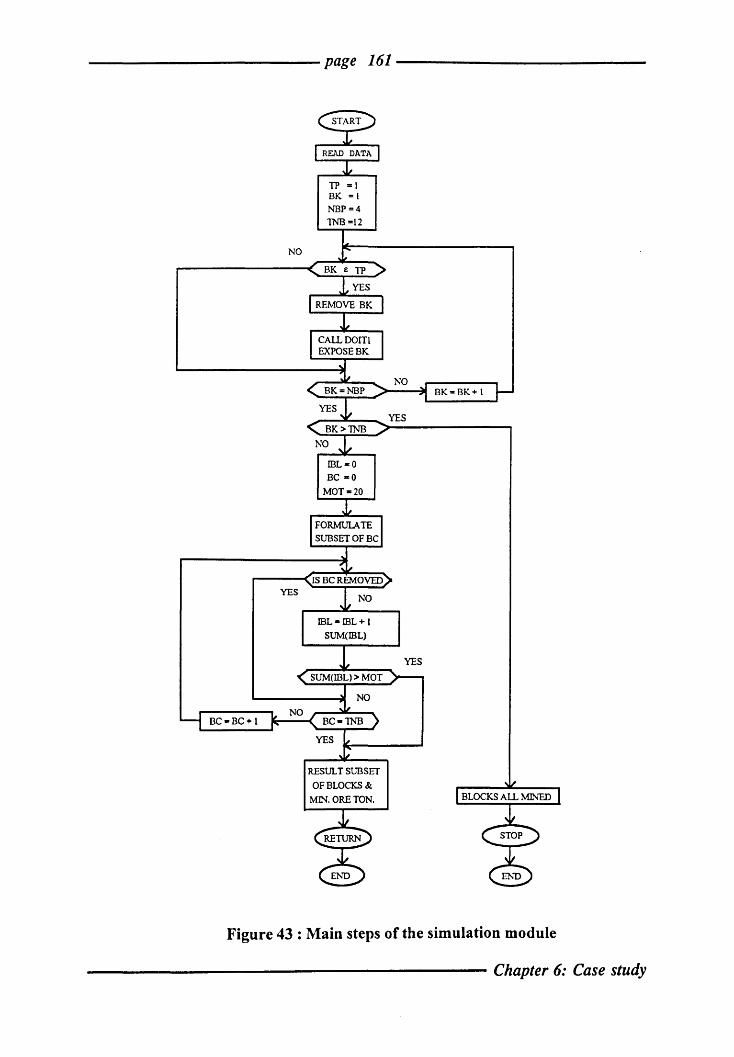
-----------------------page 161--------------------------
NO
TP =1 BK =1 NBP=4 1NB=12
NO
.__----...... YES
ffiL-O Be -0
MOT-20
~---------------
RESUL T SUBSET
OF BLOCKS &
MIN. ORE TON.
Figure 43 : Main steps of the simulation module
---------------------------- Chapter 6: Case study

------------page 162 -------------
The blocks obstructing the access to those blocks selected for removal during the
first time period of the current production period are removed. The removal of
blocks in this module is based on the usual geometrical constraints :
- a block can only be mined if the five blocks above it have already been mined
- a block is accessible only if the block above it and at least one of its
surrounding blocks have already been mined
- the slope angle of 45 degrees must be maintained
At this stage of execution the total number of blocks to be mined from the
orebody (within the waste stripping module and the LP module) represents the
scheduling of the first production period. The blocks are removed from the orebody
block model and assigned the number of the production period in which they are
removed as shown in figure 44. Only levels reached by the scheduling operation of
the total matrix are presented here to show the removed blocks for each production
period.
The development of the next subset of blocks for the LP module (production
period 2) continues starting from the last block of the optimum set of blocks
removed in the previous period, (the coordinates of the last block mined are passed
automatically to the following section).
In order to minimize equipment movements from one bench to another, the
subset is adjusted with the closest blocks to those remaining from periods 2 and 3.
The minimum ore tonnage (MOT) is then checked for the new subset of blocks
before control is returned either to the waste stripping module or to the LP module.
If the minimum ore tonnage is less than that specified, the implication is that
more stripping must be undertaken. In such cases control is returned to the stripping
module where more waste blocks are stripped. On the other hand, if the minimum
------------------ Chapter 6: Case study

------------page 163------------
ore tonnage of the blocks selected is met, the subset of blocks is submitted directly
to the LP module for further scheduling.
The original fIrst guess of the number of blocks representing the minimum ore
tonnage remains the same for all production periods unless the remaining blocks
within the optimum pit plan during the planning process are fewer than that number.
In that case control is sent to the waste stripping module, where the number of
blocks can be re-adjusted to meet the requirements.
level = 1 RIC: 1 2 3 4 5 6 7 8 9 10
1 1 1 1 1 1 1 1 1 1 1 2 1 1 1 1 1 1 1 1 1 1 3 1 1 1 1 1 1 1 1 1 1 4 1 1 1 1 1 1 1 1 1 1 5 1 1 1 1 1 1 1 1 1 1 6 1 1 1 1 1 1 1 1 1 1 7 1 1 1 1 1 1 1 1 1 1 8 1 1 1 1 1 1 1 1 1 1 9 1 1 1 1 1 1 1 1 1 1
10 1 1 1 1 1 1 1 1 1 1
Figure 44 : Coding of the blocks removed in the first production period (continued ••• )
------------------- Chapter 6: Case study

----------page 164-----------
level = 2 RIC: 1 2 3 4 5 6 7 8 9 10
1 0 0 1 0 1 1 0 0 1 1 2 0 0 0 1 0 0 1 0 0 1 3 0 0 0 1 0 0 0 0 1 0 4 1 1 0 0 0 0 0 0 1 0 5 0 0 0 1 0 1 0 0 0 0 6 1 0 0 1 1 0 0 1 1 1 7 1 1 1 0 1 0 0 0 0 1 8 0 0 1 1 0 1 0 0 1 0 9 0 1 1 1 1 0 0 0 1 0
10 1 0 1 1 0 0 0 0 0 0
level = 3 RIC: 1 2 3 4 5 6 7 8 9 10
1 10 10 10 10 10 10 10 10 10 10 2 10 0 0 0 0 0 0 0 0 10 3 10 0 0 0 0 0 0 0 0 10 4 10 0 0 0 0 0 0 0 0 10 5 10 0 0 0 0 0 0 0 0 10 6 10 0 0 0 0 0 0 0 0 10 7 10 0 0 0 0 0 0 0 0 10 8 10 0 0 0 0 0 0 0 0 10 9 10 0 1 1 0 0 0 0 0 10 10 10 10 10 10 10 10 10 10 10 10
Figure 44 ( ••• continued)
----------------- Chapter 6: Case study

-----------page 165------------
The process will then continue for the remaining production periods. The
removed blocks will always be assigned the number of the period in which they
are removed.
After a successful run of the first production period the scheduling algorithm
will continue for the next production period by iteration between the three modules
until an optimal solution is found for each period. Table 5 and table 6 show the
results of the X decision variables of the LP module for production periods 2 and 3.
Scheduling Production Period : 2
LinProg Periods 3
No of Removed Block : 36
Time Period 1 :
Time Time Period 2 : Period 3
BLOCK CO-ORDINATES I J K
243 443 543 943 253 263 963 273 473 283 383 483 583
643 743 843 353 753 853 363 463 663 373 573 673 773
343 453 553 653 953 563 763 863 973 683 693 793 893
Table 5 : Blocks produced in the second production period (continued •.• )
------------------ Chapter 6: Case study
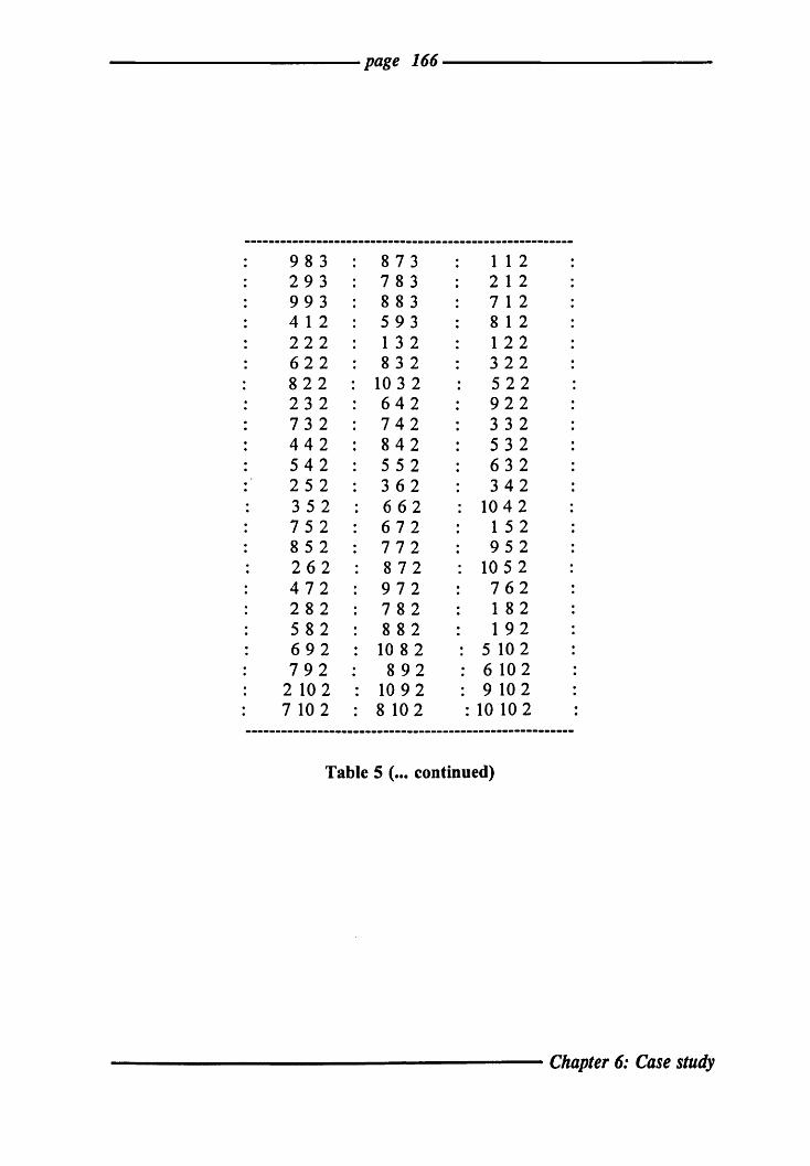
--------------------page 166---------------------
983 293 993 412 222 622 822 232 732 442 542 252 352 752 852 262 472 282 582 692 792
2 102 7 102
873 783 883 593 132 832
1032 642 742 842 552 362 662 672 772 872 972 782 882 1082 892
1092 8 102
1 1 2 212 712 812 122 322 522 922 332 532 632 342
1042 152 952
1052 762 182 192
5 102 6 102 9 102
: 10 10 2
Table 5 ( ••• continued)
----------------------- Chapter 6: Case study

---------------------page 167-----------------------
Scheduling Production Period: 3
LinProg Periods 3
No of Removed Block : 36
Time Time: Time Period 1 : Period 2 : Period 3
BLOCK CO-ORDINATES I J K
364 464 564 964 374 474 574 484 984 294 394 494 994
754 854 864 974 584 684 594 694 794 894 423 743 353
554 654 954 264 664 764 274 674 774 874 284 384 784
Table 6 : Blocks produced in the third production period (continued ••• )
---------------------------- Chapter 6: Case study

---------------------page 168-----------------------
523 623 723 823 923 433 533 733 833 933 343 643 843 853 363 463 563 373 573 883 522 922 832
753 663 863 673 773 873 973 683 783 593 693 793 893 712 132 1032 742 662 672 772 872 782 8 102
884 223 323 233 333 633 453 553 653 953 763 1 1 2 212 812 122 322 332 632 1052 762 5 102 6 102
: 10 10 2
Table 6 ( ••• continued)
The fmal coding of the removed blocks within the waste stripping and the simulation
modules during the whole scheduling process are shown in figure 45. 1,2,3 represent
the sequential removal of blocks during the three different production periods.
---------------------- Chapter 6: Case study

page 169
level = 1 RIC: 1 2 3 4 5 6 7 8 9 10
1 1 1 1 1 1 1 1 1 1 1 2 1 1 1 1 1 1 1 1 1 1 3 1 1 1 1 1 1 1 1 1 1 4 1 1 1 1 1 1 1 1 1 1 5 1 1 1 1 1 1 1 1 1 1 6 1 1 1 1 1 1 1 1 1 1 7 1 1 1 1 1 1 1 1 1 1 8 1 1 1 1 1 1 1 1 1 1 9 1 1 1 1 1 1 1 1 1 1
10 1 1 1 1 1 1 1 1 1 1
level = 2 RIC: 1 2 3 4 5 6 7 8 9 10
1 0 0 1 2 1 1 3 3 1 1 2 0 2 0 1 3 2 1 2 3 1 3 0 2 3 1 2 3 2 3 1 3 4 1 1 2 2 2 2 3 2 1 2 5 2 2 2 1 2 1 2 2 2 3 6 1 2 2 1 1 3 3 1 1 1 7 1 1 1 2 1 3 3 3 2 1 8 2 2 1 1 2 1 3 2 1 2 9 2 1 1 1 1 2 2 2 1 2
10 1 2 1 1 3 0 2 3 2 0
level = 3 RIC: 1 2 3 4 5 6 7 8 9 10
1 10 10 10 10 10 10 10 10 10 10 2 10 0 0 0 3 3 3 3 3 10 3 10 0 0 3 3 0 3 3 3 10 4 10 2 3 2 2 3 0 3 2 10 5 10 2 3 3 3 0 0 3 3 10 6 10 2 3 3 3 3 0 3 2 10 7 10 2 3 2 3 3 0 0 3 10 8 10 2 2 2 2 0 0 3 2 10 9 10 2 1 1 3 0 0 3 2 10
10 10 10 10 10 10 10 10 10 10 10
Figure 45 : Coding of the removed blocks to production periods (1,2 and 3). (continued ... )
------------------ Chapter 6: Case study

page 170
level = 4 RIC: 1 2 3 4 5 6 7 8 9 10
1 10 10 10 10 10 10 10 10 10 10 2 10 0 0 0 0 0 0 0 0 10 3 10 0 0 0 0 0 0 0 0 10 4 10 0 0 0 0 0 0 0 0 10 5 10 0 0 0 0 0 0 0 0 10 6 10 0 3 3 3 0 0 0 3 10 7 10 0 3 3 3 0 0 0 0 10 8 10 0 0 3 0 0 0 0 3 10 9 10 3 3 3 0 0 0 0 3 10
10 10 10 10 10 10 10 10 10 10 10
Figure 45 ( .•. continued)
The results of the optimised discounted alternatives, at a time value of money of
10%, are shown in table 7.
: Prod. Sched. : Discounted : Discounted : Discounted Periods Period 1: Period 2: Period 3
1 2 3
584.51 425.13 413.13
239.03 202.89 196.64
62.17 65.97 64.23
Table 7 : Discounted alternatives in each production period
It can be seen from figure 45 and table 7 that the best way of mining the
orebody is to mine the most profitable parts during the early stages of the mining
operations. Based on the above results, we can, therefore conclude that the earlier the
waste stripping is done, the more practical and profitable, scheduling becomes.
------------------- Chapter 6: Case study

------------page 171------------
However, the difficulty encountered with the Lp_solve coding is that it can
solve general LP problems up to 30,000 variables and 50,000 constraints. But solving
problems of similar size with integer variables is much more difficult. With binary
variables, Lp_solve usually provides fast answers for up to about 100 variables.
Sometimes Lp_solve can handle much larger problems, but then its success depends
critically on having a problem definition that results in a lot of integer values
immediately. Such a definition may be largely due to chance. Even commercial
codes cannot provide such a guarantee. In these cases, special codes, or heuristics
have to be resorted to.
The particular approach adopted in this research subdivides the total problem
into a number of overlapping sub-problem and finds an optimum solution to each of
these sub-problems. There is no a priori guarantee that such an approach provides
an optimum solution to the total problem.
To test the assertion that the piecewise approach provides an acceptable
solution a number of comparisons were made on a relatively large problem solved
using the approach described in this thesis and also solved using XPRESS-MP which
is a commercial, State-of-the art package devised by Proll (1995); the version
available here is capable of handling problems of up to 10,000 constraints and
15,000 variables. XPRESS-MP has two major components; a modeller and an
optimiser. The modeller takes a linear or integer linear programming problem
specified in its modelling language and produces the input file for the optimiser. The
modelling language is very powerful but requires the problem to be specified in a
completely different way to Lp_solve. In order to change the model as specified for
Lp_solve into an acceptable model for XPRESS-MP a substantial amount of expert
hand-editing was required.
An array from the case study of 1430 (e.g., 26 x 55) blocks, a maximum of
two levels open in any time period and an upper limit of two time periods in any
linear program has been considered. A simplex matrix for solution of the LP
------------------- Chapter 6: Case study
-----------page 172 ------------
module is defined equal to MAT(9,742 ; 5,720) using the waste stripping module.
The matrix was generated on GPSb (General Purpose Server). The model can
generate any mining problem size as long as enough computer memory is available.
The computer facilities available at the University of Leeds (i.e. GPS, GPSO, GPSb
(General Purpose Server), the CIF (Computationally Intensive Facility) and the Sun
servers) are more flexible with integer matrices than with real matrices.
Thus it was only possible to complete one run of the model with 9,742
constraints and 5,760 variables. For this run the optimiser required approximately 5
minutes of computer time on a Sun Sparc L workstation.
Because of the large output file of the results, only a brief output summary of
the results is described below:
The optimum solution was reached within the first iteration ( first possible
solution) and the 16th iteration ( final solution) yielding an objective function value
equal to -1694.37 which represents a net loss if the operation was carried out for the
two levels of the deposit considered.
2.5 Graphic representations
The characteristics of each pit design (metal content, total tonnage, average grade,
stripping ratio, etc ... ), are easily calculated and interpreted. It is much more difficult
to provide a representation of the approximate shape and location of the current
state of the deposit. However, pit shapes are always determined by boundaries and
these can be represented by contour plans, three-dimensional representations, cross
sectional views, etc.
------------------ Chapter 6: Case study

------------page 173 -------------
Graphic representations of the orebody and the optimal pit selected during the
optimization procedure are generated with the aid of routines from the UNIRAS
package available on the University of Leeds Sun servers.
The UNIRAS graphics package offers a wide variety of facilities which are
well documented (references and user manuals). These facilities are set up as
independent routines that perform specific functions, for example: UNIGRAPH,
UNIMAP. A graphics display on the screen as well as hard copies can be obtained
by the user.
The principal routines used in this work are:
UNIGRAPH routine: an interactive sub-program from the UNlRAS package
designed to draw hard and smooth curves, pie charts, etc... .
UNIMAP routine: an interactive sub-program from the UNIRAS package
designed to draw hard and smooth two-dimensional contours, three-dimensional and
four-dimensional views, cross-sections etc... .
These UNIRAS routines have been incorporated into a program that produces
graphics representations of the numerical data for any pit plan. All graphics display
programs developed for this research were written in Fortran 77. The user has the
choice of setting up the following figures :
1. Selection of the final pit (graph)
2. Two-dimensional contouring of mining levels
3. Three-dimensional pit representation of the optimum pit plan
4. Cross-section views of pit elevations
5. Graphics display of the part of the pit that has been mined.
------------------ Chapter 6: Case study

Q)
::J
co >
------------page 174-------------
Each graphics display routine is described In the following sections and
examples are given to illustrate their use.
2.5.1 Selection of the final pit
This routine provides a graphics representation of the optimal pit, i.e. the pit that
yields the maximum profit. The display consists of the number of pits (X-axis) and
the pit values (Y-axis) and an example is shown in figure 46.
3000
2500
/ / 2000
/ / x
/
>x· x '1-,/
/ /
/
"
>JC- ...... -x ",'
",'
.~
E 1500 ::J
Xi /
/ E .~
0.. o
1000
500
,.'
" x "x: x //
./ '" .,'
/ /
/ / x .-'X
2 3 4 5 6 7 8 9 10 11 12 13 14 15 16 17 18 19
Pit Number
Figure 46 : Selection of the final pit
-------------------- Chapter 6: Case study

------------page 175-------------
2.5.2 Two-dimensional contouring of mining levels
This routine provides a graphics display of the two-dimensional plan-contour that
represents the optimal pit limits. An example is shown in figure 47.
10-
9-
8-
7-
6-
>.. 5-
4-
3-
2-
1-
I
3 4
v 1\
I o
I
7 I R
I 9
I 10
A!Jove 3.0 _ 2.0 - 3.0
~ i.0 - 2.e _ 0.0 - 1 0
_ 3eloVlAbcve 00
[g/t]
Figure 47 : Two-dimensional contouring of mining levels
------------------- Chapter 6: Case study

------------------------page 176--------------------------
2.5.3 Three-dimensional representation of the optimum pit plan
The graphics display provided in this routine is a three-dimensional view of the
optimal pit design as shown by the example in figure 48. The angles that give the
position of the three-dimensional space representation of the pit shape (Alpha Beta
and the Distance) are set up in the source code of the routine:
x - axis represents the number of blocks in the east-west direction.
Y-axis represents the number of blocks in the north-south direction .
Z -axis represents the number of blocks in the vertical direction (the depth of
the pit)
o
Above 3.2 2.8 - 3.2
2.4 - 2.8 _ 2.0 - 2.4
E.G] 1.6 - 2.0 _ 1.2 - 1.6 _ 0.3-1.2 _ O. - 0.8
BeJow Ab ove 0.4
[gil]
Figure 48: Three-dimensional representation of the optimum pit plan
----------------------- Chapter 6: Case study

------------------------ page 177---------------------------
2.5.4 Cross-sectional views of pit elevations
The graphics display provided in this routine is a pit cross-section in the east-west
(E-W) direction. The coordinates of the cross-section are initialised in the source
code of the routine. Figure 49 shows an example of a cross-sectional disp lay in the
vertical direction.
9
8
6
x
Figure 49 : Cross-section view of pit elevations
Above 3.2
2.8 · 3.2
2.4 · 2.8 2.0 · 2.4
1.6 · 2.0
1.2 · 1.6
0.8 · 1.2 0.4 · 0.8
BelowAbove 0 .4
[g/ t]
-------------------- Chapter 6: Case study

------------page 178 -------------
2.5.5 Display of pit that has been mined
The three-dimensional representation was also extended to provide a three
dimensional view of the mined out area of the orebody. An example is shown in
figure 50.
t
Figure 50 : Display of pit that has been mined
-------------------- Chapter 6: Case study

------------page 179-------------
2.6 The validation of the methodology
The numerical accuracy of the software has been compared and demonstrated by
running the same example MAT(169 ; 324) of section 2.1 of this Chapter in the
XPRESS-MP package. Only one run was completed for one production period. The
results for the three time periods within it are shown in appendix 1, along with the
Lp_solve solution. The two solutions were identical, thus validating the piecemeal
approach.
Refering to the two given solutions, the results can best be explained by
comparing the optimum paths of blocks selected for each time period. Considering
position 2 in the value column of solution 1 and the same position in the first row
of the X decision variables of solution 2, we can see both solutions indicate that the
same block will be mined in the first time period. The corresponding co-ordinates
i=3, j=9, k=3 of this block are those shown in table 4 in the first row of the column
of the first time period. The rest of the blocks are analysed in a similar way.
The need to further validate the solution of the current study against other
methodologies from the literature and industrial practice is recognised and will need
to be pursued during further development of the software, outside this work.
3. Conclusion
The aim of the present study was to develop a mathematical model for optimizing
the schedule for the entire life of a mine. The model developed represents an
effective tool for scheduling waste and ore production for long-term planning.
The results obtained from its application on an example open pit mine
confmns the high economic effectiveness of the early user-activated waste stripping
------------------- Chapter 6: Case study
----------------------page 180------------------------
strategy with the overall objective of maximizing the profit or the Net Present Value.
The division of the entire deposit into subsets of blocks helps to reduce the size of
the mining problem in terms of computing memory and processing time as seen in
the previous sections.
The model is simple to use and can account for varying market conditions
through several parameters set by the user making parametric studies possible
without interfering with the computer code. Although the model in its present state
can only be treated as a prototype, it is fully functional and requires minimum
programming skills to operate. Developments in the area of user interface and
diagnostics will need to be made in the future.
The graphics used in the current study to depict the results are not critical to
the software, but have been incorporated for completeness of the package. They can
be extended to include the display of different windows, window menus, different
graphics representations within one run etc. Some of the routines which produce the
graphics shown in figures 46, 47, 48, 49 and 50 may have slight errors in
representing the appropriate shape when considering different data sets. Such errors
can be rectified by more precise calls of the routines, but these will not affect the
main logic of the results or even the graphics representations themselves.
The piecemeal LP methodology has been compared with a high capacity
commercial package and found to give an identical solution.
-------------------- Chapter 6: Case study
CHAPTER SEVEN
Conclusions
The growth in demand for the raw materials supplied by the mining industry has led
to the development of increasingly lower grade deposits which requires the
investment of a large amount of capital which must be repaid quickly as possible.
Many studies have shown that the combination of the time value of money and the
need to pay back the initial investment as quickly as possible require operations to
begin with a relatively high cut-off grade which then declines over the life of the
mine. Estimation of block grades and cut-off grades is thus essential for optimal
mine planning.
The aim of optimal mine planning is to determine the final pit limits for a
deposit, together with the associated grade and tonnage, which will maximize some
specified economic and! or technical criteria whist satisfying practical operational
requirements.
,
Since the advent and widespread use of computers, open pit design has been
approached by the application of many different methods and various algorithms, all
with a common objective to maximize the overall mining profit within the designed
pit limit.
The use of computers in optimal mine planning requires a model of the
deposit usually in the form of estimated block grades and tonnages. Optimal
production in such a deposit means fmding the best sequence of extracting blocks
from amongst all possible sequences. Such an operation applied to blocks within pre
determined, technically optimum pit limits will define, according to economic
criteria, the blocks which will be removed and those which will remain. As a
consequence the fmal, economically optimum, pit shape will also be defined. The
--------------------Chapter 7: Conclusions

-----------page 182 ------------
order in which the blocks are removed is said to be the optimum mining sequence
with the maximum net present value.
A large number of techniques have been applied in the search for solutions
to such planning problems. The techniques consist of both rigid operational research
methods and practical procedures which are heuristically based such as those
described in Chapter 1.
The Lerchs-Grossmann method, which overcomes the limitations of
traditional pit design, uses graph theory and always finds the optimum solution for
the case when maximum total profit is the optimising criterion. The limitation of
computing time and the difficulty in applying variable slope angles initially made the
method less popular than the sub-optimal moving cone method, though the Whittle
4-D package has overcome some of these difficulties.
The Korobov and the corrected Korobov methods give good results. The
method uses cones to defme the shape of the pit. The cones can be arranged in any
desired manner so that a realistic pit shape can be obtained. The optimum pit is the
best combination of these cones. The great advantage of these methods is their
relative simplicity and the rapid generation of solutions. Although it is not possible
to provide a rigorous proof that the corrected form of the Korobov algorithm will
always yield the optimal solution no counter example has yet been found.
A single pit design based on a fixed set of costs, prices and cut-off grades
can often provide a misleading picture of the possible working pit and of the
mineable reserves. It is always advisable to test the sensitivity of the pit design to
changes in all of the variables used to calculate the revenue block model. In
addition, it is also advisable to test the sensitivity of the pit design to grade and
tonnage estimation errors. These types of analyses could result in the need to
generate several dozen pit designs each of which could take significant computing
time. The problem is that optimal open pit design algorithms do not express the
-------------------Chapter 7: Conclusions

-----------page 183------------
solution parametrically, i.e. as a function of the parameters that were used to
calculate the block model or of other design parameters such as wall slopes. A
parametric solution to optimal open pit design, based on something other than simple
metal content might eventually lead to a direct method of solving the problem of
maximum net present value.
An alternative approach used in this thesis is to parameterize the pit design
as a function of a number of variables. This algorithm, which uses grade values
instead of revenue values, is based on techniques of functional analysis. The aim
of this method is to transform a parametric optimization problem with severe
geometric constraints into a simple one with no constraints; it does not take any
economic parameters into account.
This technique could also be applied for the determination of mining
sequences for the optimization of the recoverable reserves of any particular pit,
where in economic terms the mining sequence is more important during the early
stages and plays a major role in capital investment.
However, the objective of parameterization is to find a complete family of
technically optimal pits corresponding to every possible value of the total tonnage
and the selected tonnage. The only drawback is the limitation of the slope angle of
the cone.
The characteristics associated with each pit design, such as metal content,
total tonnage, average grade, stripping ratio and other information are provided in
the form of data fIles that can be used for post-processing. Graphics views (contours,
two-dimensional and three-dimensional) are also provided.
The method is not rigorous, and has some weaknesses on the economic side
when compared to other economic or revenue based algorithms. However,
parameterization appears to be at least as good as most algorithms and better than
--------------------Chapter 7: Conclusions

-----------page 184 ------------
many in respect of the computing time.
The selection of the optimum pit amongst the set of pits produced by the
parameterization method is obtained using a simple profit function. The application
of the profit function to each block generates a block profit matrix. Pit profit is
obtained by summing the profit of each block mined within that pit limit. The
definition (selection) of an optimum pit is taken to be the configuration of blocks
whose pit profit is a maximum.
Production scheduling is of vital importance for the operating efficiency of
an open pit mine and is the last operation in optimal open pit design. A major
problem in production scheduling is the determination of a mining sequence which
satisfies the physical and economic constraints whilst ensuring a continuous feed to
the mill in such a way as to maximize the Net Present Value.
The optimum schedule depends on both physical and economic parameters
which can be considered together or separately. Considering both parameters at the
same time is computationally time consuming and, for large problems as the
number of states increases, the solution may be impossible to attain.
In many cases the application of a single operational research technique limits
the solution to a problem, especially when a rigorous optimum is required for a
problem which is subject to strict constraints. In recent years there has been a
tendency to combine two or more different operational research methods to solve
complicated mine planning problems. These techniques have included dynamic
programming, computer simulation and interactive techniques, oriented graph
simulation, simulation and linear programming.
Such combinations of operational research techniques can split the problem
into two parts. In this case one part uses linear programming to find the optimum
path, whilst the other part checks the feasibility of the first solution in terms of
--------------------Chapter 7: Conclusions

----------------------page 185-----------------------
mining constraints and improves the scheduling sequence. The effect of this check
is that the fmal linear programming solution will always be confined to blocks which
become accessible during the period under consideration.
The idea of 'free ore" develops the above consideration further. By
submitting to the linear programming optimization only those blocks which are
immediately available for mining, the constraints on precedence and accessibility of
blocks can be eliminated. Such an approach cannot lead to a rigorous overall
optimum in the mathematical sense but the solution is very close to such an
optimum.
Techniques such as linear programming suffer from the "curse of
dimensionality" as the size of the problem increases it rapidly becomes impossible
to handle the number of variables. The author has solved this problem by
minimizing the numbers of variables and constraints at each stage, using a
combination of linear programming with interactive simulation. The user-activated
waste stripping module which is applied at the start of operations reduces the size
of the problem during the execution of the software. This module increases the
accessibility of ore blocks which then reduces the number of elements (constraints)
inside the linear programming matrix.
Such a formulation allows the determination of an optimal mine schedule
using the criterion of maximum Net Present Value. It is believed that the algorithms
used will yield a true practical optimum or a solution which is very close to the true
optimum (the results presented in Chapter 6 demonstrate this). At present the
algorithm described is limited to a workstation implementation but it is believed that
the use of decomposition methods and approximate solution algorithms for the linear
programming component will ultimately yield a PC version.
Examples of the results obtained from the programs together with tables and
figures representing removed blocks in each period and their discounted values are
--------------------Chapter 7: Conclusions

------------page 186-------------
given in detail in Chapter 6. The quick and accurate results that can be generated
by this computer program should lead to a much more flexible approach to optimal
open pit design and scheduling and thereby improve economic performance.
-------------------Chapter 7: Conclusions

References and bibliography
Albach, H. (1967) Long-range planning in open-pit mining. Management service,
Vol. 13, 1967, pp. B549-568.
Bellman, R. (1957) Dynamic programming. Princeton Press, Princeton, New Jersey,
342p.
Blackwell, M.R.L. (1970) Some Aspects of the Evaluation and Planning of the
Bougainville Copper Project, Decision-making in the Mineral Industry, Montreal
C.I.M., pp. 261-269.
Boyce, W.P. (1969) Open pit planning using a computer. AMDEL Bulletin No.8,
pp.59-77. October.
Bronson, R. (1989) Theory and Problems of Matrix Operations, Book Published by
McGraw-hill, Inc.
Coleou, T. (1989) Technical parameterization of reserves for open pit design and
mining planning. In 21st Symposium on the application of computers and operations
research in the mineral industries (APCOM) (Littleton, Colorado: AIME, 1989),
485-94.
Dagdelen, K. and Francois-Bongarcon, D. (1982) Towards the complete double
parameterization of recovered reserves in open pit mining. 17th APCOM, p1584-
1589.
Dantzig, G.B. (1963) Linear programming and extensions. Princeton University
Press, Princeton, N.J., 1963.
-----------------~References and bibliography

------------page 188 -------------
David, M., Dowd, P.A. and Korobov, S. (1974) Forecasting departure from
planning in open pit design and grade control. In 12th symposium on the application
of computers and operations reseach in the mineral industries (APCOM) Volume 2
(Golden, Colo: Colorado School of Mines), F131-42 1974.
Dowd, P.A. (1976) Application of dynamic and stochastic programming to optimize
cutoff grades and production rates". Trans. Inst. Min. Metall., Section A, volume
85, October 1976, A22-A31.
Dowd, P .A. and David, M. (1976) Planning from estimates : sensitivity of mine
production schedules to estimation methods. Advanced geostatistics in the mining
industry NATO ASI SERIES C: Mathematical and Physical Sciences volume 24,
eds. Guarascio, M., David, M. and Huijbregts, C. D. Reidel Pub. Co. Dordrecht,
Netherlands, 163-183.
Dowd, P.A. (1980) The role of certain taxation systems in the management of
mineral resources. National and international management of mineral resources ed.
M.J. Jones, IMM, London, 329-335.
Dowd, P.A. and Elvan, L. (1987) Dynamic Programming applied to Grade Control
in Sub-level Open Stopping. Trans. Inst. Min. Metall., Section A, volume 96,
October 1987, AI71-AI78.
Dowd, P.A. (1989) The solution of large scale linear programming problems in the
mining industry. Leeds University Mining Association (LUMA) Journal, 1989, pp.
85-90.
Dowd, P.A. and Onur, A.H. (1993) Open pit optimization: I Optimal open pit
design. Trans. Inst. Min. Metall. (Sect. A: Min. industry), 102, May-August 1993,
pp. A95-AI04. The Institution of Mining and Metallurgy 1993.
-----------------~B.eferences and bibliography

-----------page 189 ------------
Dowd, P.A. and Onur, A.H. (1992) Optimizing open pit design and sequencing.
23rd Symposium on the application of computers and operations research in the
mineral industries (APCOM). AIME, Littleton, Co. 411-422.
Dowd, P.A. (1992) A short course in optimal open pit design. Course notes for a
course given for Gencor Ltd., South Africa.
Dowd, P .A. (1994a) The optimal design of quarries. In Whateley, M.K.G. and
Harvey, P .K. (eds) Mineral Resource Evaluation II: methods and case histories,
Geological Society Special Publication No. 79, 141-155.
Dowd, P.A. (1994b) Optimal open pit design: Sensitivity to estimated block values.
In Whateley, M.K.G. and Harvey, P.K. (eds) Mineral Resource Evaluation II:
methods and case histories, Geological Society Special Publication No. 79, 87-94.
Erickson, J.D. and Pana, M.T. (1966) Preparation of short-range mining plans by
computer at the Utah Mine of Kennecott Copper Co-orporation. Scientific and
Engineering Computer Center Report, Kennecott Copper Co-orporation, Salt Lake
City, Utah, 1966.
Fran~ois-Bongar~on, D. and Marechal, A. (1976) A new method for optimum pit
design : parameterization of the final pit contour. In 14th Symposium on the
application of computers and operations research in the mineral industries
(APCOM), (New York: AIME, 1976) 573-83.
Fran~ois-Bongar~on, D. (1978) Le parametrage des contours optimaux d'une
exploitation a ciel ouvert, These pour obtenir Ie grade de Docteur-Ingenieur.
L'Institut National Poly technique de Lorraine, France.
----------------~References and bibliography

----------------------page 190------------------------
Francois-Bongarcon, D., Guibal D. (1980) "Open-Pit Optimization by
Parameterization of the Final Pit Contour: New Advances and Applications", in
Proc. 18th Int. APCOM. Symp., Moscow, U.S.S.R., October 20-25 1980.
Francois-Bongarcon, D. and Guibal, D. (1981) "Parameterization of Optimal
Designs of an Open Pit - Beginning of a New Phase of Research, Trans, SME,
AIME, Vol. 274, pp 1801-1805.
Francois-Bongarcon, D., and Guibal, D., (1982), Algorithms for parameterizing
reserves under different geometrical constraints. In the 17th Symposium on the
application of computers and operations research in the mineral industries
(APCOM) (New York: AIME, 1982), pp.297-309.
Fytas, K. Hadjigeorgiou, J. and Collins, J.L. (1993) Production scheduling
optimization in open pit mines. International Journal of Surface Mining and
Reclamation, (1993) : 1-9.
Garey, M.R. and Johnson, D.S. (1979) Computers and intractability: a guide to the
theory of NP-completeness. Freeman, San Francisco, USA.
Hartman, R.I. and Varma, G.C. (1966) A three-dimensional optimum pit program
and a basis for mining engineering system. Proc. Sixth Annual Symposium on
Computers and Operations Research in the Mineral Industries, (1966).
Huang, S. (1993) Optimization of open pit mining sequence with a computerized
model. In Trans. Inst. Min. Metall. (Sec. A : Min. Industry), 102, May-August
1993.
Johnson. T.B. (1968) Optimum open pit mine production scheduling. Operations
Research Center Report, ORC 68-11, University of California, Berkeley (PhD
Thesis) (May 1968).
------------------References and bibliography

-----------------------page 191-------------------------
Johnson, T.B. and Sharp, W.R. (1971) A three-dimensional dynamic programming
method for optimal open pit design. Rep. Invest. U.S. Bur. Mines 7553, 1971, 25p.
Korobov, S. (1974) Method for determining optimal open pit limits. Technical report
EP74-R-4, Ecole Poly technique de Monreal, 1974.
Lane, K.J. (1964) Choosing the optimum cut-off grade. Colorado School of Mines
quarterly Vol. 59 p811-829.
Lerchs, H. and Grossmann, I.P. (1965) Optimum design of open pit mines. CIM
Bulletin, 58, 47-54.
Matheron, G. (1975a) Complements sur Ie parametrage des contours optimaux. Note
Geostatistique no. 129 Centre de Geostatistique et de Morphologie Methematique,
Internal Report N-401, Fontainebleau, France, 1975, 54p.
Matheron, G. (1975b) Parametrage de contours optimaux. Note Geostatistique no.
128 Centre de Geostatistique et de Morphologie Mathematique, Internal report N-
403, Fontainebleau, France, 1975, 54p.
Matheron, G. (197 5c) Le parametrage technique des reserves. Note Geostatistique
no. 134 Centre de Goestatistique et de Morphologie, Internal Report N-453 ,
Fontainebleau, France, 1975, 54p.
Moks, D.J. (1983) Parameterization for open pit mining. Leeds University Mining
Association (LUMA), Department of Mining and Mineral Engineering, Leeds
University, 1983.
Moks, D.J. (1983) The application of computers to open pit limits analysis. PhD
thesis, Department of Mining and Mineral Engineering, University of Leeds.
----------------~R.eferences and bibliography

-----------page 192------------
Onur, A.H. (1992) Optimal open pit design and planning. PhD thesis, Department
of Mining and Mineral Engineering, University of Leeds.
Onur, A.H. and Dowd, P.A. (1993) Open pit optimization - part 2: production
scheduling and inclusion of roadways. Trans. IMM, Vol. 102, 1993, pp. AI05-
A113.
Proll, L.G. (1995) Revised simplex method subroutine, School of Computer Studies
Leeds University, England U.K.
Roman, R.J. (1973) The use of dynamic programming for determining mine-mill
production schedules. Application of computer methods in the minerals industry
(Johannesburg: SAIMM, 1973), pp. 165-170.
Roman, R.J. (1974) The role of time value of money in determining an open pit
mining sequence and pit limits. In 12th Symposium on the application of computers
and operations research in the mineral industries (APCOM) (Golden, Colo :
Colorado School of Mines I AIME, 1974), C72-85.
Stuart, N.J. (1992) Pit optimization using solid modelling and the Lerchs-Grossmann
algorithm. Int. J. Surface Mining and Reclamation. Vol. 6, no. 1, pp. 19-30.
Taylor, H.K. (1972) General Background Theory of Cut-off Grades, Institution of
Mining and Metallurgy Transaction, July 1972, pp. AI60-179.
UNIRAS package (1989) (UNIRAS Reference and User Manuals) UNIRAS A/S 376
Gladsaxevej, DK-2860 Scf>borg, Denmark.
Whittle, J. (1989) The facts and fallacies of open pit optimization. Whittle
Programming Pty., Ltd., North Balwyn, Victoria, Australia, 1989.
-----------------~B.eferences and bibliography

------------page 193 -------------
Whittle, J. (1988) Beyond Optimization in Open Pit Design. Presented at the First
Canadian Conference on Computer Applications in the Mineral Industry. Laval
University, Quebec City, March 7-9, 1988. Whittle Programming Pty. Ltd.
Melbourne, Australia.
Wilke, F.L. and Reimer, T.H. (1979) Optimizing the short term production schedule
for an open pit iron ore mining operation. Computer Methods for the 80's. AIME,
New York. pp. 642-647.
Wilke, F.L. Mueller, K. and Wright, E. (1984) Ultimate pit limit and production
scheduling optimization. In 18th symposium on the application of computer and
operations research in the mineral industries (APCOM) (London: IMM, 1984), 29-
38.
Wright, E.A. (1989) Dynamic programming in open pit mining sequence planning
a case study, In the 21st Symposium on the application of computers and operations
research in the mineral industries (APCOM) (New York, NY: AIME, 1989),
pp.415-422.
Zhang, Y.D. Cheng, Y.D. and Su, J. (1993) Application of goal programming in
open pit planning. International Journal of Surface Mining and Reclamation 7 (1993)
pp. 41-45.
------------------References and bibliography

APPENDIX ONE
Comparison of the results from the XPRESS-MP
package and the lp_solve
1. XPRESS-MP package solution 1
The following is the solution produced by the XPRESS-MP package. The results are
for one production period and three time periods in one linear program run. The key
words in the following solution are :
BS - is the basic variable,
LL - is the lower limit, and
UL - is the upper limit.
Value - status of blocks (0. not mined, 1. mined)
Problem Statistics
Matrix mtrx2
Objective OBJ
RHS RHSOOOOI
Problem has 169 rows and 324 structural columns
Solution Statistics
Maximisation perfonned
Optimal solution found after 2 iterations
Objective function value is 867.420000
Columns Section
Appendix 1: comparison of results

page 195
Number Column At Value Input Cost Reduced Cost
C 170 x 001 BS .000000 7.690000 .000000 C 171 x 002 BS 1.000000 7.210000 .000000 C 172 x 003 BS 1.000000 28.720000 .000000 C 173 x 004 UL .000000 6.910000 -.080000 C 174 x 005 LL .000000 2.480000 .720000 C 175 x 006 LL .000000 3.120000 .550000 C 176 x 007 BS .000000 3.120000 .000000 C 177 x 008 BS .000000 9.730000 .000000 C 178 x 009 LL .000000 2.080000 .640000 C 179 x 010 LL .000000 3.850000 .480000 C 180 x 011 UL 1.000000 15.900000 -.620000 C 181 x 012 BS .000000 7.730000 .000000 C 182 x 013 UL 1.000000 28.720000 -1.780000 C 183 x 014 BS 1.000000 9.190000 .000000 C 184 x 015 LL .000000 4.070000 .450000 C 185 x 016 LL .000000 2.090000 .640000 C 186 x 017 BS 1.000000 15.470000 .000000 C 187 x 018 UL 1.000000 9.730000 -.050000 C 188 x 019 LL .000000 1.380000 .700000 C 189 x 020 LL .000000 8.590000 .050000 C 190 x 021 LL .000000 -.660000 .890000 C 191 x 022 BS 1.000000 27.590000 .000000 C 192 x 023 LL .000000 1.330000 .920000 C 193 x 024 BS 1.000000 9.190000 .000000 C 194 x 025 UL 1.000000 10.090000 -.090000 C 195 x 026 BS 1.000000 9.190000 .000000 C 196 x 027 LL .000000 2.090000 .790000 C 197 x 028 BS 1.000000 9.730000 .000000 C 198 x 029 LL .000000 6.110000 .090000 C 199 x 030 BS .000000 9.190000 .000000 C 200 x 031 LL .000000 3.190000 .590000 C 201 x 032 UL 1.000000 68.310000 -5.380000 C 202 x 033 LL .000000 .480000 .780000 C 203 x 034 LL .000000 3.120000 .610000 C 204 x 035 LL .000000 8.500000 .060000 C 205 x 036 LL .000000 7.210000 .170000 C 206 x 037 UL 1.000000 14.560000 -.500000 C 207 x 038 LL .000000 6.350000 .260000 C 208 x 039 BS 1.000000 37.530000 .000000 C 209 x 040 BS 1.000000 37.530000 .000000 C 210 x 041 LL .000000 -1.300000 1.380000 C 211 x 042 BS .000000 7.730000 .000000 C 212 x 043 LL .000000 8.690000 .040000 C 213 x 044 LL .000000 2.480000 .720000
Appendix 1: comparison of results

page 196
C 214 x 045 LL .000000 3.120000 .550000 C 215 x 046 LL .000000 3.120000 .550000 C 216 x 047 UL 1.000000 9.730000 -.050000
C 217 x 048 LL .000000 2.270000 .760000
C 218 x 049 LL .000000 1.520000 .880000
C 219 x 050 LL .000000 7.690000 .130000
C 220 x 051 BS .000000 7.210000 .000000
C 221 x 052 UL 1.000000 14.560000 -.500000
C 222 x 053 LL .000000 6.350000 .050000
C 223 x 054 BS 1.000000 9.730000 .000000
C 224 x 055 BS .000000 7.690000 .000000
C 225 x 056 BS 1.000000 9.190000 .000000
C 226 x 057 LL .000000 2.270000 .630000
C 227 x 058 LL .000000 -.600000 1.260000 C 228 x 059 LL .000000 9.190000 .000000
C 229 x 060 LL .000000 4.070000 .450000
C 230 x 061 LL .000000 2.090000 .790000
C 231 x 062 UL 1.000000 15.470000 -.570000
C 232 x 063 BS 1.000000 9.730000 .000000
C 233 x 064 LL .000000 .650000 1.040000
C 234 x 065 LL .000000 3.600000 .520000
C 235 x 066 BS 1.000000 9.870000 .000000
C 236 x 067 BS 1.000000 9.470000 .000000
C 237 x 068 BS 1.000000 15.900000 .000000
C 238 x 069 BS .000000 9.190000 .000000
C 239 x 070 BS 1.000000 10.090000 .000000
C 240 x 071 BS .000000 9.190000 .000000 C 241 x 072 LL .000000 2.090000 .640000 C 242 x 073 BS 1.000000 9.730000 .000000 C 243 x 074 LL .000000 3.120000 .550000
C 244 x 075 LL .000000 2.520000 .710000
C 245 x 076 LL .000000 2.270000 .630000
C 246 x 077 BS .000000 6.910000 .000000
C 247 x 078 UL 1.000000 15.250000 -.550000
C 248 x 079 LL .000000 3.120000 .610000
C 249 x 080 LL .000000 8.500000 .060000
C 250 x 081 BS .000000 7.210000 .000000
C 251 x 082 BS 1.000000 14.560000 .000000
C 252 x 083 LL .000000 6.350000 .050000
C 253 x 084 UL 1.000000 9.190000 .000000
C 254 x 085 LL .000000 2.180000 .640000
C 255 x 086 LL .000000 2.090000 .640000 C 256 x 087 UL 1.000000 15.470000 -.570000 C 257 x 088 BS .000000 6.910000 .000000 C 258 x 089 LL .000000 2.480000 .610000
C 259 x 090 LL .000000 3.120000 .550000
Appendix 1: comparison of results

page 197
C 260 x 091 BS 1.000000 3.120000 .000000
C 261 x 092 BS 1.000000 9.730000 .000000
C 262 x 093 BS .000000 2.270000 .000000
C 263 x 094 LL .000000 8.200000 .090000
C 264 x 095 BS .000000 7.690000 .000000
C 265 x 096 BS .000000 7.210000 .000000
C 266 x 097 UL 1.000000 28.720000 -1.780000
C 267 x 098 BS .000000 6.910000 .000000
C 268 x 099 UL 1.000000 9.730000 -.050000 C 269 x 100 LL .000000 7.690000 .130000 C 270 x 101 BS 1.000000 9.190000 .000000
C 271 x 102 LL .000000 2.270000 .760000 C 272 x 103 LL .000000 -.600000 1.260000
C 273 x 104 LL .000000 2.270000 .630000
C 274 x 105 BS .000000 7.690000 .000000
C 275 x 106 LL .000000 6.910000 .200000
C 276 x 107 LL .000000 .080000 1.140000
C 277 x 108 LL .000000 2.180000 .780000
C 278 x 109 BS 1.000000 6.990000 .000000
C 279 x 110 BS .000000 6.550000 .000000
C 280 x 111 LL .000000 26.110000 1.000000
C 281 x 112 BS 1.000000 6.280000 .000000
C 282 x 113 LL .000000 2.260000 .110000
C 283 x 114 BS .000000 2.840000 .000000
C 284 x 115 UL 1.000000 2.840000 -.245000
C 285 x 116 BS 1.000000 8.850000 .000000
C 286 x 117 BS .000000 1.890000 .000000
C 287 x 118 BS .000000 3.500000 .000000
C 288 x 119 BS .000000 14.450000 .000000
C 289 x 120 UL 1.000000 7.030000 -.130000
C 290 x 121 BS .000000 26.110000 .000000
C 291 x 122 LL .000000 8.360000 .000000
C 292 x 123 UL 1.000000 3.700000 -.010000
C 293 x 124 BS .000000 1.900000 .000000
C 294 x 125 LL .000000 14.070000 .570000
C 295 x 126 BS .000000 8.850000 .000000
C 296 x 127 BS .000000 1.250000 .000000
C 297 x 128 BS 1.000000 7.810000 .000000
C 298 x 129 BS .000000 -.600000 .000000
C 299 x 130 LL .000000 25.080000 1.680000
C 300 x 131 LL .000000 1.210000 .210000
C 301 x 132 LL .000000 8.360000 .000000
C 302 x 133 BS .000000 9.170000 .000000
C 303 x 134 LL .000000 8.360000 .000000
C 304 x 135 LL .000000 1.900000 .150000
C 305 x 136 LL .000000 8.850000 .050000
Appendix 1: comparison of results

page 198
C 306 x 137 UL 1.000000 5.550000 -.180000 C 307 x 138 UL 1.000000 8.360000 .000000 C 308 x 139 LL .000000 2.900000 .050000 C 309 x 140 BS .000000 62.100000 .000000 C 310 x 141 BS .000000 .430000 .000000 C 311 x 142 LL .000000 2.830000 .070000 C 312 x 143 BS 1.000000 7.730000 .000000 C 313 x 144 BS 1.000000 6.550000 .000000 C 314 x 145 BS .000000 13.230000 .000000 C 315 x 146 BS 1.000000 5.780000 .000000 C 316 x 147 LL .000000 34.120000 2.580000 C .317 x 148 LL .000000 34.120000 2.580000 C 318 x 149 LL .000000 -1.180000 .430000 C 319 x 150 UL 1.000000 7.030000 -.130000 C 320 x 151 BS 1.000000 7.900000 .000000 C 321 x 152 LL .000000 2.260000 .110000 C 322 x 153 BS .000000 2.840000 .000000 C 323 x 154 BS .000000 2.840000 .000000 C 324 x 155 BS .000000 8.850000 .000000 C 325 x 156 LL .000000 2.070000 .130000 C 326 x 157 LL .000000 1.380000 .190000 C 327 x 158 BS 1.000000 6.990000 .000000 C 328 x 159 UL 1.000000 6.550000 -.170000 C 329 x 160 BS .000000 13.230000 .000000 C 330 x 161 UL 1.000000 5.780000 -.210000 C 331 x 162 LL .000000 8.850000 .050000 C 332 x 163 UL 1.000000 6.990000 -.130000 C 333 x 164 LL .000000 8.360000 .000000 C 334 x 165 BS .000000 2.070000 .000000 C 335 x 166 LL .000000 -.540000 .370000 C 336 x 167 BS 1.000000 8.360000 .000000 C 337 x 168 UL 1.000000 3.700000 -.010000 C 338 x 169 LL .000000 1.900000 .150000 C 339 x 170 BS .000000 14.070000 .000000 C 340 x 171 LL .000000 8.850000 .050000 C 341 x 172 LL .000000 .590000 .270000 C 342 x 173 LL .000000 3.270000 .020000 C 343 x 174 LL .000000 8.980000 .060000 C 344 x 175 LL .000000 8.610000 .030000 C 345 x 176 LL .000000 14.450000 .620000 C 346 x 177 BS 1.000000 8.360000 .000000
C 347 x 178 LL .000000 9.170000 .090000 C 348 x 179 UL 1.000000 8.360000 .000000 C 349 x 180 BS .000000 1.900000 .000000 C 350 x 181 LL .000000 8.850000 .050000 C 351 x 182 BS .000000 2.840000 .000000
Appendix 1: comparison of results

page 199
C 352 x 183 LL .000000 2.290000 .110000 C 353 x 184 BS .000000 2.070000 .000000 C 354 x 185 UL 1.000000 6.280000 -.200000 C 355 x 186 BS .000000 13.870000 .000000 C 356 x 187 LL .000000 2.830000 .070000 C 357 x 188 BS 1.000000 7.730000 .000000 C 358 x 189 UL 1.000000 6.550000 -.170000 C 359 x 190 LL .000000 13.230000 .500000 C 360 x 191 UL 1.000000 5.780000 -.210000 C 361 x 192 BS .000000 8.360000 .000000 C 362 x 193 BS .000000 1.990000 .000000 C 363 x 194 BS .000000 1.900000 .000000 C 364 x 195 BS .000000 14.070000 .000000 C 365 x 196 UL 1.000000 6.280000 -.200000 C 366 x 197 BS .000000 2.260000 .000000 C 367 x 198 BS 1.000000 2.840000 .000000 C 368 x 199 LL .000000 2.840000 .060000 C 369 x 200 LL .000000 8.850000 .050000 C 370 x 201 BS 1.000000 2.070000 .000000 C 371 x 202 BS 1.000000 7.460000 .000000 C 372 x 203 UL 1.000000 6.990000 -.130000 C 373 x 204 BS 1.000000 6.550000 .000000 C 374 x 205 BS .000000 26.110000 .000000 C 375 x 206 UL 1.000000 6.280000 -.200000 C 376 x 207 BS .000000 8.850000 .000000 C 377 x 208 BS 1.000000 6.990000 .000000 C 378 x 209 LL .000000 8.360000 .000000 C 379 x 210 LL .000000 2.070000 .130000 C 380 x 211 LL .000000 -.540000 .370000 C 381 x 212 BS .000000 2.070000 .000000 C 382 x 213 UL 1.000000 6.990000 -.130000 C 383 x 214 BS 1.000000 6.280000 .000000 C 384 x 215 LL .000000 .070000 .320000 C 385 x 216 LL .000000 1.990000 .140000 C 386 x 217 LL .000000 6.350000 .190000 C 387 x 218 LL .000000 5.960000 .340000 C 388 x 219 LL .000000 23.740000 3.050000 C 389 x 220 LL .000000 5.710000 .120000 C 390 x 221 BS 1.000000 2.050000 .000000 C 391 x 222 BS 1.000000 2.580000 .000000 C 392 x 223 BS .000000 2.580000 .000000 C 393 x 224 LL .000000 8.040000 .185000 C 394 x 225 UL 1.000000 1.720000 -.150000 C 395 x 226 BS 1.000000 3.180000 .000000 C 396 x 227 LL .000000 13.140000 .990000 C 397 x 228 LL .000000 6.390000 .190000
Appendix 1: comparison of results

page 200
C 398 x 229 LL .000000 23.740000 2.050000 C 399 x 230 LL .000000 7.600000 .440000 C 400 x 231 BS .000000 3.370000 .000000 C 401 x 232 UL 1.000000 1.730000 -.150000 C 402 x 233 LL .000000 12.790000 1.530000 C 403 x 234 LL .000000 8.040000 .490000 C 404 x 235 UL 1.000000 1.140000 -.210000 C 405 x 236 LL .000000 7.100000 .390000 C 406 x 237 UL 1.000000 -.550000 -.370000 C 407 x 238 LL .000000 22.800000 3.640000 C 408 x 239 BS 1.000000 1.100000 .000000 C 409 x 240 LL .000000 7.600000 .440000 C 410 x 241 LL .000000 8.340000 .510000 C 411 x 242 LL .000000 7.600000 .440000 C 412 x 243 BS 1.000000 1.730000 .000000 C 413 x 244 LL .000000 8.040000 .540000 C 414 x 245 BS .000000 5.050000 .000000 C 415 x 246 LL .000000 7.600000 .440000 C 416 x 247 BS 1.000000 2.630000 .000000 C 417 x 248 LL .000000 56.450000 5.330000 C 418 x 249 UL 1.000000 .390000 -.280000 C 419 x 250 BS 1.000000 2.580000 .000000 C 420 x 251 LL .000000 7.030000 .380000 C 421 x 252 LL .000000 5.960000 .270000 C 422 x 253 LL .000000 12.030000 .880000 C 423 x 254 LL .000000 5.250000 .210000 C 424 x 255 LL .000000 31.010000 5.370000 C 425 x 256 LL .000000 31.010000 5.370000 C 426 x 257 BS 1.000000 -1.070000 .000000 C 427 x 258 LL .000000 6.390000 .190000 C 428 x 259 LL .000000 7.180000 .400000 C 429 x 260 BS 1.000000 2.050000 .000000 C 430 x 261 UL 1.000000 2.580000 -.060000 C 431 x 262 UL 1.000000 2.580000 -.060000 C 432 x 263 LL .000000 8.040000 .490000 C 433 x 264 BS 1.000000 1.880000 .000000 C 434 x 265 BS 1.000000 1.250000 .000000 C 435 x 266 LL .000000 6.350000 .320000 C 436 x 267 LL .000000 5.960000 .100000 C 437 x 268 LL .000000 12.030000 .880000 C 438 x 269 BS .000000 5.250000 .000000 C 439 x 270 LL .000000 8.040000 .540000 C 440 x 271 LL .000000 6.350000 .190000 C 441 x 272 LL .000000 7.600000 .440000 C 442 x 273 UL 1.000000 1.880000 -.130000 C 443 x 274 BS 1.000000 -.490000 .000000
Appendix 1: comparison oj results

page 201
C 444 x 275 LL .000000 7.600000 .440000 C 445 x 276 BS .000000 3.370000 .000000 C 446 x 277 BS 1.000000 1.730000 .000000 C 447 x 278 LL .000000 12.790000 .960000 C 448 x 279 LL .000000 8.040000 .540000 C 449 x 280 BS 1.000000 .540000 .000000 C 450 x 281 BS 1.000000 2.970000 .000000 C 451 x 282 LL .000000 8.160000 .560000 C 452 x 283 LL .000000 7.830000 .490000 C 453 x 284 LL .000000 13.140000 1.610000 C 454 x 285 LL .000000 7.600000 .440000 C 455 x 286 LL .000000 8.340000 .600000 C 456 x 287 LL .000000 7.600000 .440000 C 457 x 288 UL 1.000000 1.730000 -.150000 C 458 x 289 LL .000000 8.040000 .540000 C 459 x 290 UL 1.000000 2.580000 -.060000 C 460 x 291 BS 1.000000 2.080000 .000000 C 461 x 292 UL 1.000000 1.880000 -.130000 C 462 x 293 LL .000000 5.710000 .050000 C 463 x 294 LL .000000 12.610000 .940000 C 464 x 295 BS 1.000000 2.580000 .000000 C 465 x 296 LL .000000 7.030000 .380000 C 466 x 297 LL .000000 5.960000 .100000 C 467 x 298 LL .000000 12.030000 1.380000 C 468 x 299 BS .000000 5.250000 .000000 C 469 x 300 LL .000000 7.600000 .440000 C 470 x 301 UL 1.000000 1.810000 -.140000 C 471 x 302 UL 1.000000 1.730000 -.150000 C 472 x 303 LL .000000 12.790000 .960000 C 473 x 304 LL .000000 5.710000 .050000 C 474 x 305 UL 1.000000 2.050000 -.110000 C 475 x 306 BS .000000 2.580000 .000000 C 476 x 307 BS .000000 2.580000 .000000 C 477 x 308 LL .000000 8.040000 .540000 C 478 x 309 BS .000000 1.880000 .000000 C 479 x 310 LL .000000 6.780000 .360000 C 480 x 311 LL .000000 6.350000 .190000 C 481 x 312 LL .000000 5.960000 .270000 C 482 x 313 LL .000000 23.740000 2.050000 C 483 x 314 LL .000000 5.710000 .050000 C 484 x 315 LL .000000 8.040000 .490000 C 485 x 316 LL .000000 6.350000 .320000 C 486 x 317 LL .000000 7.600000 .440000 C 487 x 318 BS 1.000000 1.880000 .000000 C 488 x 319 BS 1.000000 -.490000 .000000 C 489 x 320 UL 1.000000 1.880000 -.130000
Appendix 1: comparison of results

page 202
C 490 x 321 LL .000000 6.350000 .190000 C 491 x 322 LL .000000 5.710000 .250000 C 492 x 323 BS 1.000000 .070000 .000000 C 493 x 324 BS 1.000000 1.810000 .000000
2. Lp_solve solution 2
The following is the solution produced by Lp_solve. The results are for one production
period for three time periods in one linear program run. There is a total number of324
variables, with 108 variables per time period.
Objective function value is : 867.42
The X decision variables (0 and 1 for blocks not mined and mined) are :
X= 0 1 1 0 0 0 000 0 1 0 1 1 0 0 1 1 0 0 0 1 0 0 1 0 0 1 0 0 0 1
o 0 0 0 1 0 1 1 0 000 0 0 100 0 0 1 0 1 0 000 1 001 100 1 1
1 1 1 101 0 0 0 0 1 000 101 001 000 1 100 0 0 101 010
o 0 0 0 001 0 0 1 001 1 000 I 0 0 1 0 0 0 0 1 000 1 0 1 001
1 0 0 0 0 1 101 000 1 100 0 0 0 0 1 101 0 1 1 000 1 0 0 0 0
o 0 0 0 0 000 0 000 1 001 1 0 1 000 0 1 0 1 001 1 1 101 0
1 0 0 0 0 1 100 0 000 1 100 1 1 000 0 0 100 1 0 1 0 1 000
1 000 101 1 0 0 0 0 0 0 100 1 1 101 1 0 000 0 0 0 1 100 1
001 1 0 0 0 000 1 011 100 1 0 0 000 1 100 1 0 0 000 0 0
o 0 0 0 0 1 1 100 1 1
The co-ordinates of the mined blocks (unit = 1) for each time period are shown in table
4 Chapter6.
-------------- Appendix 1: comparison of results


![Telecommunication Products - Trendtek jointing pits.pdf · [01] UG2006 - P6 Pit UG2007 - P7 Pit UG2008 - P8 Pit UG2900 - P9 Pit UG2001 - P1 Pit UG2002 - P2 Pit UG2003 - P3 Pit UG2004](https://img.dokumen.tips/doc/110x75/5a7969077f8b9ab9308d3433/telecommunication-products-jointing-pitspdf01-ug2006-p6-pit-ug2007-p7-pit.jpg)