Interactive Design Space Exploration and Optimization … · shape space while geometry and physical ... Interactive Design Space Exploration and ... Interactive Design Space Exploration

Interactive Design Space Exploration and Optimization for CAD Models

ADRIANA SCHULZ, JIE XU, and BO ZHU, Massachusetts Institute of TechnologyCHANGXI ZHENG and EITAN GRINSPUN, Columbia UniversityWOJCIECH MATUSIK, Massachusetts Institute of Technology

Smooth interpolations

Interactive Exploration

Optimization

min stress

Precomputed Samples

CAD System

ParametricSpace

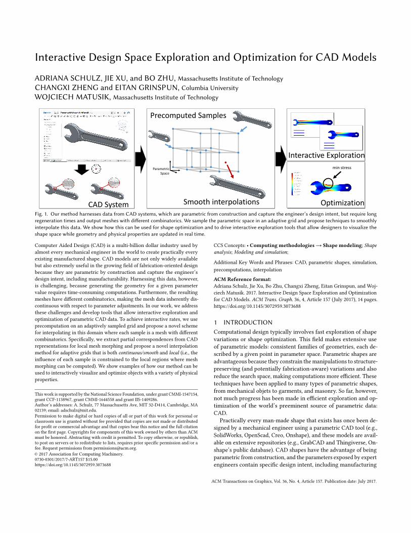
Fig. 1. Our method harnesses data from CAD systems, which are parametric from construction and capture the engineer’s design intent, but require longregeneration times and output meshes with different combinatorics. We sample the parametric space in an adaptive grid and propose techniques to smoothlyinterpolate this data. We show how this can be used for shape optimization and to drive interactive exploration tools that allow designers to visualize theshape space while geometry and physical properties are updated in real time.

Computer Aided Design (CAD) is a multi-billion dollar industry used by

almost every mechanical engineer in the world to create practically every

existing manufactured shape. CAD models are not only widely available

but also extremely useful in the growing field of fabrication-oriented design

because they are parametric by construction and capture the engineer’s

design intent, including manufacturability. Harnessing this data, however,

is challenging, because generating the geometry for a given parameter

value requires time-consuming computations. Furthermore, the resulting

meshes have different combinatorics, making the mesh data inherently dis-

continuous with respect to parameter adjustments. In our work, we address

these challenges and develop tools that allow interactive exploration and

optimization of parametric CAD data. To achieve interactive rates, we use

precomputation on an adaptively sampled grid and propose a novel scheme

for interpolating in this domain where each sample is a mesh with different

combinatorics. Specifically, we extract partial correspondences from CAD

representations for local mesh morphing and propose a novel interpolation

method for adaptive grids that is both continuous/smooth and local (i.e., theinfluence of each sample is constrained to the local regions where mesh

morphing can be computed). We show examples of how our method can be

used to interactively visualize and optimize objects with a variety of physical

properties.

This work is supported by the National Science Foundation, under grant CMMI-1547154,

grant CCF-1138967, grant CMMI-1644558 and grant IIS-1409286.

Author’s addresses: A. Schulz, 77 Massachusetts Ave, MIT 32-D414, Cambridge, MA

02139; email: [email protected].

Permission to make digital or hard copies of all or part of this work for personal or

classroom use is granted without fee provided that copies are not made or distributed

for profit or commercial advantage and that copies bear this notice and the full citation

on the first page. Copyrights for components of this work owned by others than ACM

must be honored. Abstracting with credit is permitted. To copy otherwise, or republish,

to post on servers or to redistribute to lists, requires prior specific permission and/or a

fee. Request permissions from [email protected].

© 2017 Association for Computing Machinery.

0730-0301/2017/7-ART157 $15.00

https://doi.org/10.1145/3072959.3073688

CCS Concepts: • Computing methodologies→ Shape modeling; Shapeanalysis; Modeling and simulation;

Additional Key Words and Phrases: CAD, parametric shapes, simulation,

precomputations, interpolation

ACM Reference format:Adriana Schulz, Jie Xu, Bo Zhu, Changxi Zheng, Eitan Grinspun, and Woj-

ciech Matusik. 2017. Interactive Design Space Exploration and Optimization

for CAD Models. ACM Trans. Graph. 36, 4, Article 157 (July 2017), 14 pages.

https://doi.org/10.1145/3072959.3073688

1 INTRODUCTIONComputational design typically involves fast exploration of shape

variations or shape optimization. This field makes extensive use

of parametric models: consistent families of geometries, each de-

scribed by a given point in parameter space. Parametric shapes are

advantageous because they constrain themanipulations to structure-

preserving (and potentially fabrication-aware) variations and also

reduce the search space, making computations more efficient. These

techniques have been applied to many types of parametric shapes,

from mechanical objets to garments, and masonry. So far, however,

not much progress has been made in efficient exploration and op-

timization of the world’s preeminent source of parametric data:

CAD.

Practically every man-made shape that exists has once been de-

signed by a mechanical engineer using a parametric CAD tool (e.g.,

SolidWorks, OpenScad, Creo, Onshape), and these models are avail-

able on extensive repositories (e.g., GrabCAD and Thingiverse, On-

shape’s public database). CAD shapes have the advantage of being

parametric from construction, and the parameters exposed by expert

engineers contain specific design intent, including manufacturing

ACM Transactions on Graphics, Vol. 36, No. 4, Article 157. Publication date: July 2017.

https://doi.org/10.1145/3072959.3073688

https://doi.org/10.1145/3072959.3073688

157:2 • A. Schulz et. al.

constraints (see Figure 2). Parametric CAD allows for many inde-

pendent variables but these are typically constrained for structure

preserving consideration, the need to interface with other parts,

and manufacturing limitations. In this context, engineers typically

expose a small number of variables which can be used to optimize

the shape.

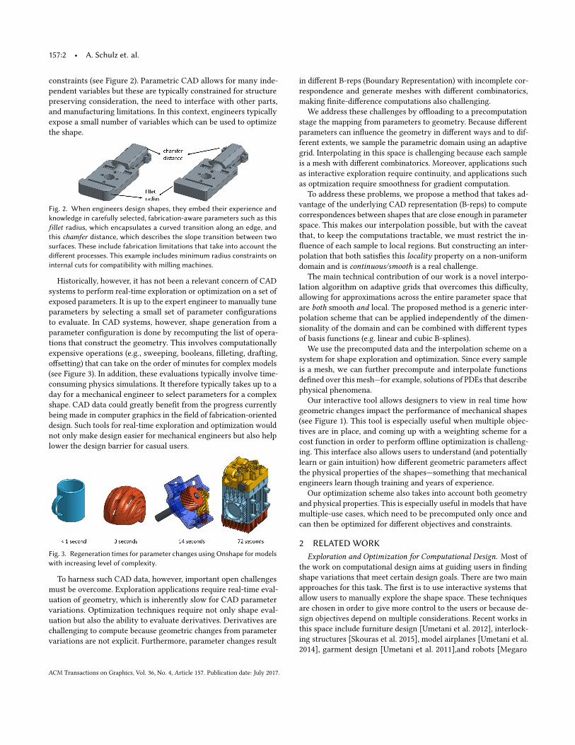
Fig. 2. When engineers design shapes, they embed their experience andknowledge in carefully selected, fabrication-aware parameters such as thisfillet radius, which encapsulates a curved transition along an edge, andthis chamfer distance, which describes the slope transition between twosurfaces. These include fabrication limitations that take into account thedifferent processes. This example includes minimum radius constraints oninternal cuts for compatibility with milling machines.

Historically, however, it has not been a relevant concern of CAD

systems to perform real-time exploration or optimization on a set of

exposed parameters. It is up to the expert engineer to manually tune

parameters by selecting a small set of parameter configurations

to evaluate. In CAD systems, however, shape generation from a

parameter configuration is done by recomputing the list of opera-

tions that construct the geometry. This involves computationally

expensive operations (e.g., sweeping, booleans, filleting, drafting,

offsetting) that can take on the order of minutes for complex models

(see Figure 3). In addition, these evaluations typically involve time-

consuming physics simulations. It therefore typically takes up to a

day for a mechanical engineer to select parameters for a complex

shape. CAD data could greatly benefit from the progress currently

being made in computer graphics in the field of fabrication-oriented

design. Such tools for real-time exploration and optimization would

not only make design easier for mechanical engineers but also help

lower the design barrier for casual users.

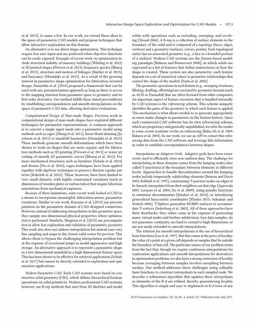
Fig. 3. Regeneration times for parameter changes using Onshape for modelswith increasing level of complexity.

To harness such CAD data, however, important open challenges

must be overcome. Exploration applications require real-time eval-

uation of geometry, which is inherently slow for CAD parameter

variations. Optimization techniques require not only shape eval-

uation but also the ability to evaluate derivatives. Derivatives are

challenging to compute because geometric changes from parameter

variations are not explicit. Furthermore, parameter changes result

in different B-reps (Boundary Representation) with incomplete cor-

respondence and generate meshes with different combinatorics,

making finite-difference computations also challenging.

We address these challenges by offloading to a precomputation

stage the mapping from parameters to geometry. Because different

parameters can influence the geometry in different ways and to dif-

ferent extents, we sample the parametric domain using an adaptive

grid. Interpolating in this space is challenging because each sample

is a mesh with different combinatorics. Moreover, applications such

as interactive exploration require continuity, and applications such

as optmization require smoothness for gradient computation.

To address these problems, we propose a method that takes ad-

vantage of the underlying CAD representation (B-reps) to compute

correspondences between shapes that are close enough in parameter

space. This makes our interpolation possible, but with the caveat

that, to keep the computations tractable, we must restrict the in-

fluence of each sample to local regions. But constructing an inter-

polation that both satisfies this locality property on a non-uniform

domain and is continuous/smooth is a real challenge.

The main technical contribution of our work is a novel interpo-

lation algorithm on adaptive grids that overcomes this difficulty,

allowing for approximations across the entire parameter space that

are both smooth and local. The proposed method is a generic inter-

polation scheme that can be applied independently of the dimen-

sionality of the domain and can be combined with different types

of basis functions (e.g. linear and cubic B-splines).

We use the precomputed data and the interpolation scheme on a

system for shape exploration and optimization. Since every sample

is a mesh, we can further precompute and interpolate functions

defined over this mesh—for example, solutions of PDEs that describe

physical phenomena.

Our interactive tool allows designers to view in real time how

geometric changes impact the performance of mechanical shapes

(see Figure 1). This tool is especially useful when multiple objec-

tives are in place, and coming up with a weighting scheme for a

cost function in order to perform offline optimization is challeng-

ing. This interface also allows users to understand (and potentially

learn or gain intuition) how different geometric parameters affect

the physical properties of the shapes—something that mechanical

engineers learn though training and years of experience.

Our optimization scheme also takes into account both geometry

and physical properties. This is especially useful in models that have

multiple-use cases, which need to be precomputed only once and

can then be optimized for different objectives and constraints.

2 RELATED WORKExploration and Optimization for Computational Design. Most of

the work on computational design aims at guiding users in finding

shape variations that meet certain design goals. There are two main

approaches for this task. The first is to use interactive systems that

allow users to manually explore the shape space. These techniques

are chosen in order to give more control to the users or because de-

sign objectives depend on multiple considerations. Recent works in

this space include furniture design [Umetani et al. 2012], interlock-

ing structures [Skouras et al. 2015], model airplanes [Umetani et al.

2014], garment design [Umetani et al. 2011],and robots [Megaro


Interactive Design Space Exploration and Optimization for CAD Models • 157:3

et al. 2015], to name a few. In our work, we extend these ideas to

the space of parametric CAD models and propose techniques that

allow interactive exploration on this domain.

An alternative is to use direct shape optimization. This technique

require less user input and are preferred when objective functions

can be easily exposed. Example of recent work on optimization in-

clude structural stability of masonry buildings [Whiting et al. 2012]

or 3D printed shapes [Prévost et al. 2013], frequency spectra [Bharaj

et al. 2015], structure and motion of linkages [Bächer et al. 2015],

and buoyancy [Musialski et al. 2015]. As a result of the growing

interest in parametric shape optimization for fabrication-oriented

design, Musialski et al. [2016] proposed a framework that can be

used with any parametrization approach as long as there is access

to the mapping function from parameter space to geometry and its

first order derivative. Our method fulfills these stated preconditions

by establishing correspondences and smooth interpolations on the

space of parametric CAD data, allowing derivative evaluations.

Computational Design of Man-made Shapes. Previous work in

computational design of man-made shapes have exploited different

techniques for parametric representations. A common approach

is to convert a single input mesh into a parametric model using

methods such as cages [Zheng et al. 2011], linear blend skinning [Ja-

cobson et al. 2011] or manifold harmonics [Musialski et al. 2015].

These methods generate smooth deformations which have been

shown to work on shapes that are more organic and for fabrica-

tion methods such as 3D printing [Prévost et al. 2013] or water jet

cutting of smooth 2D parametric curves [Bharaj et al. 2015]. For

more mechanical structures such as furniture [Schulz et al. 2014]

and drones [Du et al. 2016], cages techniques have been applied

together with algebraic techniques to preserve discrete regular pat-

terns [Bokeloh et al. 2012]. These, however, have been limited to

very small datasets, with highly constrained variations (such as

dimensions of wooden plates or carbon tubes) that require laborious

annotations from mechanical engineers.

Because of these limitations, some recent work looked at CAD as

a means to incorporate meaningful, fabrication-aware, parametric

variations. Similar to our work, Koyama et al. [2015] use precom-

putation on the parametric domain of CAD designed connectors.

However, instead of addressing interpolation in this geometric space,

they sample one-dimensional physical properties where optimiza-

tion is performed. Similarly, Shugrina et al. [2015] use precomputa-

tion to allow fast exploration and validation of parametric geometry.

This work also does not address interpolation but instead uses very

fine sampling and snaps to the closest valid vertex for preview. This

allows them to bypass the challenging interpolation problem but

at the expense of occasional jumps in model appearance and high

storage. An alternative approach is to represent a parametric shape

as a low dimensional manifold in a high dimensional feature space.

This has been shown to be effective for retrieval applications [Schulz

et al. 2017] but cannot be directly extended to exploration and opti-

mization applications.

Modern Parametric CAD. Early CAD systems were based on con-

structive solid geometry (CSG), which defines hierarchical boolean

operations on solid primitives. Modern professional CAD systems,

however, use B-rep methods that start from 2D sketches and model

solids with operations such as extruding, sweeping, and revolv-

ing [Stroud 2006]. A B-rep is a collection of surface elements in the

boundary of the solid and is composed of a topology (faces, edges,

vertices) and a geometry (surfaces, curves, points). Each topological

entity has an associated geometry (e.g., a face is a bounded portion

of a surface). Modern CAD systems use the feature-based model-

ing paradigm [Bidarra and Bronsvoort 2000], in which solids are

expressed as a list of features that define instructions on how the

shape is created. These system are also parametric: each feature

depends on a set of numerical values or geometric relationships that

control the shape of the models [Farin et al. 2002].

The geometric operations in each feature (e.g., sweeping, booleans,

filleting, drafting, offsetting) are executed by geometric kernels (such

as ACIS or Parasolid) that are often licensed from other companies.

An important aspect of feature execution that is handled internally

by CAD systems is the referencing scheme. This scheme uniquely

identifies the parts of the geometry to which each feature is applied.

This mechanism is what allows models to re-generate appropriately

as users make changes in parameters in the feature history. Since

each commercial CAD software has its own referencing scheme,

which are proprietary and generally unpublished, we refer the reader

to some recent academic works on referencing [Baba-Ali et al. 2009;

Bidarra et al. 2005]. In our work, we use an API to extract this refer-

encing data from the CAD software and leverage this information

in order to establish correspondences between shapes.

Interpolation on Adaptive Grids. Adaptive grids have been exten-

sively used to efficiently store non-uniform data. The challenge for

interpolating in these domains comes from the hanging nodes (also

called T-junctions) at the boundary between elements at different

levels. Approaches to handle discontinuities around the hanging

nodes include temporarily subdividing elements [Benson and Davis

2002; Kobbelt et al. 1997], constraining T-junction nodes on edges to

be linearly interpolated from their neighbors on that edge [Agarwala

2007; Losasso et al. 2004; Xu et al. 2009], using penalty functions

to minimize discontinuities [Setaluri et al. 2014], or introducing

generalized barycentric coordinates [Floater 2015; Sukumar and

Malsch 2006]. T-Splines generalize NURBS surfaces to accommo-

date T-vertices [Sederberg et al. 2003]. All of these approaches have

their drawbacks: they either come at the expense of generating

many virtual nodes and further subdivision, lose data samples, do

not guarantee continuity, are hard to extend to high dimensions, or

are not easily extended to smooth interpolations.

The solution for smooth interpolations is the use of hierarchical

basis functions [Lee et al. 1997]. But this comes at the price of locality:

the value of a point at a given cell depends on samples that lie outside

the boundary of that cell. The particular nature of our problem stems

from the fact that, though we require continuous interpolations for

exploration applications and smooth interpolations for derivatives

in optimization problems, we also have a strong restriction of locality

because averaging between samples involves morphing between

meshes. Our method addresses these challenges using refinable

basis functions to construct interpolants in each sampled node. We

describe a refinement algorithm that updates these interpolants

as elements of the K-d are refined, thereby guaranteeing locality.

This algorithm is simple and easy to implement in K-d trees of any



dimension or grading. Most importantly, it can be implemented with

multiple basis functions, allowing not just continuous but smoothapproximations.

3 WORKFLOWThe workflow of our system is shown in Figure 1. In an offline

phase, CAD shapes are precomputed by adaptively sampling the

parametric domain. Interpolating basis functions for each sample

(Section 5) and compatible meshes for interpolation (Section 6) are

computed during this phase. For some applications, in addition to

storing the geometry at each sample, we also precompute and store

different simulation results.

For exploration, we use the typical user interface with sliders

for interactively modifying shape parameters (see top-right corner

of Figure 1). Both geometry and precomputed physical properties

are interpolated in real time and displayed. For this application, we

use a continuous interpolation function to avoid flickering when

switching between regions of the adaptive grid. For optimization, we

use smooth interpolations for evaluation of continuous derivatives.

4 PRECOMPUTATION OVERVIEW AND NOTATIONSA parametric shape is defined as a function that returns a geometry

for each parameter configuration x ∈ A, where A is the feasible

parameter set. Here and henceforth we assume that a sample value

pk at xk ∈ A can be evaluated by interfacing with a CAD system

and consists of a tetrahedral mesh. Our method computes an ap-

proximation P(x) of the parametric shape by interpolating these

samples.

We use a K-d tree in parameter space for sampling and interpo-

lation (see Figure 1). We use the term element to refer to the cells

of the K-d tree. The parametric shape is sampled at every corner of

every element. To each sample xk we associate a basis functionψkand approximate the shape by interpolating the samples:

P(x) =∑k

pkψk (x). (1)

Definition 1 (Support). The support of each basis function S(ψk ) isdefined as region on which it assumes non-zero values.

The challenge with computing the above sum is that pk are

meshes with varying combinatorics. To address this, let us assume a

canonical mesh pl for each element el . Then, if x ∈ el , we can com-

pute P l (x) by converting each sample xk whose support contains

el to this canonical mesh plk :

P l (x) =∑

k,el ∈S (ψk )

plkψk (x). (2)

To keep this problem tractable, we would like to limit the support of

the basis functions. To this end, we make the following definitions.

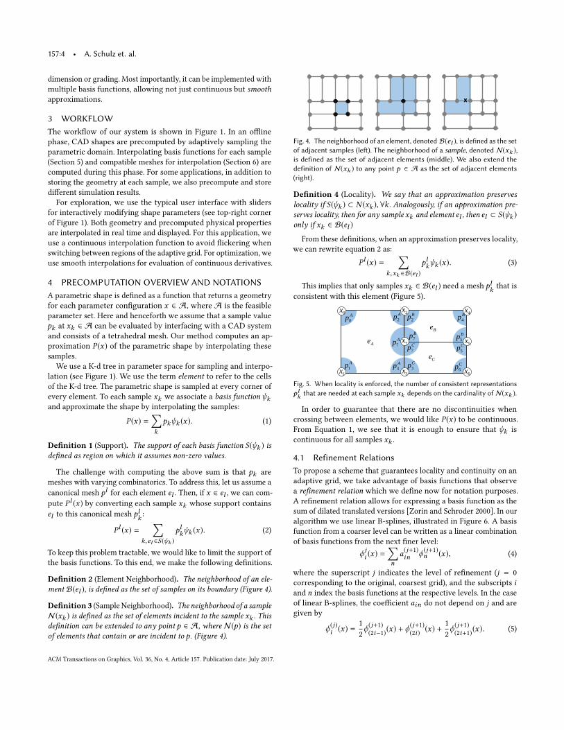
Definition 2 (Element Neighborhood). The neighborhood of an ele-ment B(el ), is defined as the set of samples on its boundary (Figure 4).

Definition 3 (Sample Neighborhood). The neighborhood of a sampleN(xk ) is defined as the set of elements incident to the sample xk . Thisdefinition can be extended to any point p ∈ A, where N(p) is the setof elements that contain or are incident to p. (Figure 4).

x

Fig. 4. The neighborhood of an element, denoted B(el ), is defined as the setof adjacent samples (left). The neighborhood of a sample, denoted N(xk ),is defined as the set of adjacent elements (middle). We also extend thedefinition of N(xk ) to any point p ∈ A as the set of adjacent elements(right).

Definition 4 (Locality). We say that an approximation preserveslocality if S(ψk ) ⊂ N (xk ),∀k . Analogously, if an approximation pre-serves locality, then for any sample xk and element el , then el ⊂ S(ψk )only if xk ∈ B(el )

From these definitions, when an approximation preserves locality,

we can rewrite equation 2 as:

P l (x) =∑

k,xk ∈B(el )

plkψk (x). (3)

This implies that only samples xk ∈ B(el ) need a mesh plk that is

consistent with this element (Figure 5).

Ce

Be

Ae Ap7

Bp7

Cp7

Bp2

Cp5

Cp3Cp6

Ap2Ap0

Ap3

Ap1

Bp4

Bp5

0x

1x

2x4x

5x

3x

7x

6x

Fig. 5. When locality is enforced, the number of consistent representationsplk that are needed at each sample xk depends on the cardinality of N(xk ).

In order to guarantee that there are no discontinuities when

crossing between elements, we would like P(x) to be continuous.

From Equation 1, we see that it is enough to ensure that ψk is

continuous for all samples xk .

4.1 Refinement RelationsTo propose a scheme that guarantees locality and continuity on an

adaptive grid, we take advantage of basis functions that observe

a refinement relation which we define now for notation purposes.

A refinement relation allows for expressing a basis function as the

sum of dilated translated versions [Zorin and Schroder 2000]. In our

algorithm we use linear B-splines, illustrated in Figure 6. A basis

function from a coarser level can be written as a linear combination

of basis functions from the next finer level:

ϕji (x) =

∑n

a(j+1)

in ϕ(j+1)n (x), (4)

where the superscript j indicates the level of refinement (j = 0

corresponding to the original, coarsest grid), and the subscripts iand n index the basis functions at the respective levels. In the case

of linear B-splines, the coefficient ain do not depend on j and are

given by

ϕ(j)i (x) =

1

2

ϕ(j+1)

(2i−1)(x) + ϕ

(j+1)

(2i) (x) +1

2

ϕ(j+1)

(2i+1)(x). (5)



0

00

11

01

21

11

31

1

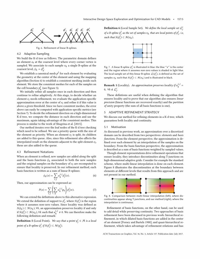
Fig. 6. Refinement of linear B-splines.

4.2 Adaptive SamplingWe build the K-d tree as follows. The parametric domain defines

an element e0 at the coarsest level where every corner vertex is

sampled. We associate to each sample xk a single B-spline at the

coarsest level,ψk = ϕ0

k .

We establish a canonical mesh pl for each element by evaluating

the geometry at the center of the element and using the mapping

algorithm (Section 6) to establish a consistent meshing inside each

element. We store the consistent meshes for each of the samples on

the cell boundary plk (see Figure 5).

We initially refine all samples once in each direction and then

continue to refine adaptively. At this stage, to decide whether an

element el needs refinement, we evaluate the application-specific

approximation error at the center of el and refine it if this value is

above a given threshold. Since we have consistent meshes, the error

above can easily be computed with application-specific metrics (see

Section 7). To decide the refinement direction on a high-dimensional

K-d tree, we compute the distance in each direction and use the

maximum, again taking advantage of the consistent meshes. This

process is similar to the work of Shugrina et al. [2015].

Our method iterates over the leaf nodes of the K-d tree checking

which need to be refined. We use a priority queue with the size of

the element as priority. When an element el is split, its childrenare added to this queue. Also, since this refinement also affects the

interpolated result on the elements adjacent to the split element el ,these are also added to the queue.

4.3 Refinement NotationsWhen an element is refined, new samples are added along the split

and the basis functions ψk associated to both the new samples

and the original samples on the boundary of el are recomputed to

ensure that locality is preserved. In our refinement method, each

basis function is written as a sum of linear B-splines:

ψk (x) =∑i, j

αi, jk ϕ

ji (x). (6)

Then, our approximation can be expressed as:

P(x) =∑i, j

(∑k

αi, jk pk

)ϕji (x). (7)

We can extend the definitions above to this alternative expression.

We extend the definition of support to ϕji , where S(ϕ

ji ) is the region

where it assumes non-zero values. Since locality was defined as

S(ψk ) ⊂ N (xk ),∀k , an approximation preserves locality if and only

if S(ϕji ) ⊂ N(xk ),∀k such that a

i, jk , 0. We can therefore make the

following definition and remark:

Definition 5 (Local Point). We say that a point yij ∈ A is a local

point of a B-spline ϕ ji if S(ϕji ) ⊂ N(yij ).

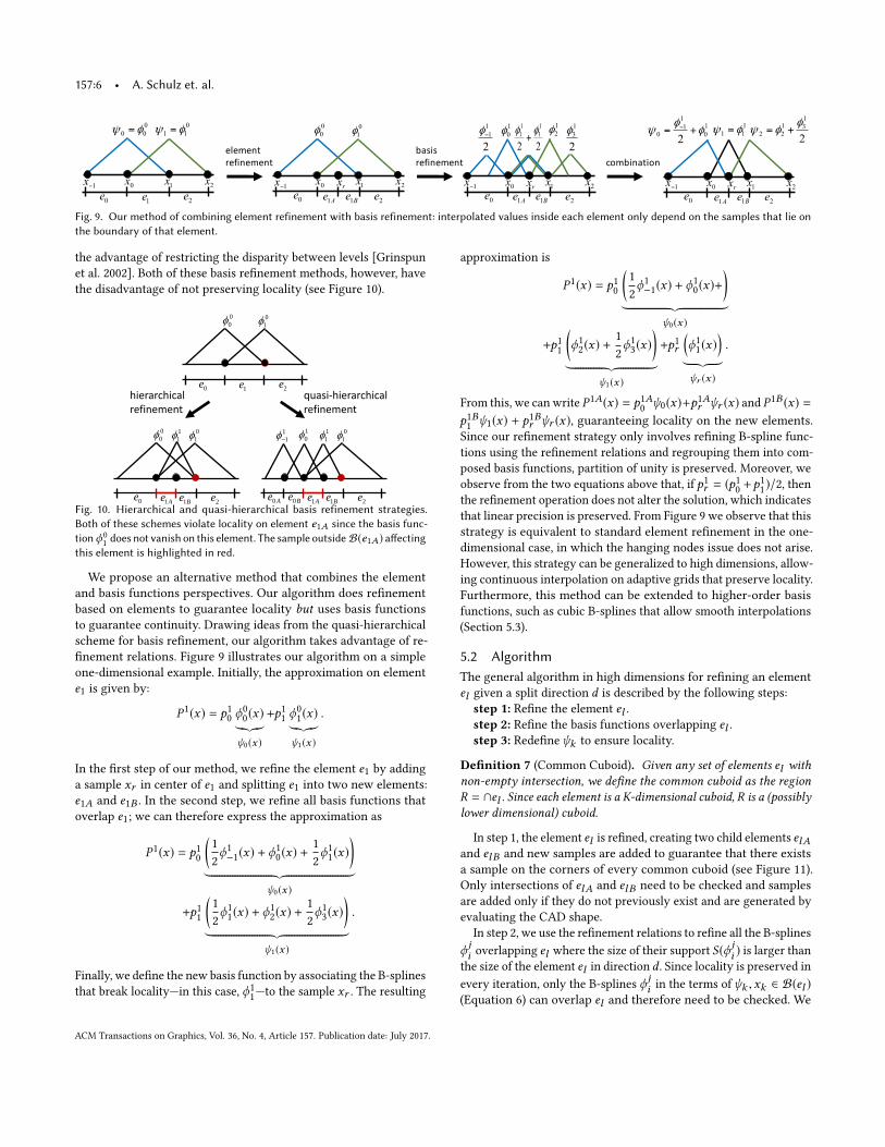
Definition 6 (Local Sample Set). We define the local sample set Lij

of a B-spline ϕ ji as the set of samples xk that are local points of ϕ ji , i.e,such that S(ϕ ji ) ⊂ N(xk ).

x

Fig. 7. A linear B-spline ϕ ji is illustrated in blue: the blue "‘x"’ is the centerand the region where it assumes non-zero values is shaded in light blue.The local sample set of this linear B-spline L(ϕ ji ), is defined as the set of

samples xk such that S (ϕ ji ) ⊂ N(xk ) and is illustrated in black.

Remark 1 (Locality). An approximation preserves locality if α i, jk =

0, ∀k < Lij .

These defintions are useful when defining the algorithm that

ensures locality and to prove that our algorithm also ensures linearprecision (linear functions are recovered exactly) and the partitionof unity property (the sum of all basis functions is one).

5 ADAPTIVE REFINEMENT STRATEGYWe discuss our method for refining elements in a K-d tree, which

guarantees both locality and continuity.

5.1 MotivationAs discussed in previous work, an approximation over a discretized

domain can be described from two perspectives: elements and basisfunctions. From the element perspective, the approximation is de-

fined over each element by an interpolation of the samples on the

boundary. From the basis function perspective, the approximation

is described as a sum of basis functions weighted by sampled values.

Though element representations drive refinement operations that

ensure locality, they introduce discontinuities along T-junctions on

high-dimensional adaptive grids. Consider for example the standard

scheme, where multi-linear interpolation is done on each element.

Figure 8 illustrates the discontinuities at the boundary between

elements at different levels that results from this approach and are

not present in our method.

Fig. 8. Comparison between multi-linear interpolation (left), where dis-continuities appear along T-junctions, and our method (right), where theinterpolation is continuous.

Refinement of basis functions, on the other hand, can be used

to add detail while preserving continuity. Two approaches of basis

refinement have been discussed in previous work: hierarchical re-

finement, in which dilated basis functions are added in the center

of an element [Forsey and Bartels 1988]; and quasi-hierarchical re-

finement, which takes advantage of refinement relations and has



00φ

01φ

2e0e

elementrefinement

000 φψ =

0e 1e 2e

011 φψ = 1

0φ12φ

2

11−φ

22

11

11 φφ+

2

13φ

Ae1 2e0e

10

11

0 2φ

φψ += −

2e0e

111 φψ =

2

131

22φ

φψ +=

basisrefinement combination

0x rx 1xBe1

1−x 2x0x rx 1x1−x 2x 0x rx 1x1−x 2xAe1 Be1Ae1 Be1

0x 1x1−x 2x

Fig. 9. Our method of combining element refinement with basis refinement: interpolated values inside each element only depend on the samples that lie onthe boundary of that element.

the advantage of restricting the disparity between levels [Grinspun

et al. 2002]. Both of these basis refinement methods, however, have

the disadvantage of not preserving locality (see Figure 10).

0

00

1

0

00

11

11

00

11

11

1

0e1e 2e

Ae1 2eBe1Ae0 Be0Ae1 2eBe10e

hierarchical refinement

quasi-hierarchical refinement

Fig. 10. Hierarchical and quasi-hierarchical basis refinement strategies.Both of these schemes violate locality on element e1A since the basis func-tionϕ0

1does not vanish on this element. The sample outside B(e1A) affecting

this element is highlighted in red.

We propose an alternative method that combines the element

and basis functions perspectives. Our algorithm does refinement

based on elements to guarantee locality but uses basis functionsto guarantee continuity. Drawing ideas from the quasi-hierarchical

scheme for basis refinement, our algorithm takes advantage of re-

finement relations. Figure 9 illustrates our algorithm on a simple

one-dimensional example. Initially, the approximation on element

e1 is given by:

P1(x) = p1

0ϕ0

0(x)︸︷︷︸

ψ0(x )

+p1

1ϕ0

1(x)︸︷︷︸

ψ1(x )

.

In the first step of our method, we refine the element e1 by adding

a sample xr in center of e1 and splitting e1 into two new elements:

e1A and e1B . In the second step, we refine all basis functions that

overlap e1; we can therefore express the approximation as

P1(x) = p1

0

(1

2

ϕ1

−1(x) + ϕ1

0(x) +

1

2

ϕ1

1(x)

)︸︷︷︸

ψ0(x )

+p1

1

(1

2

ϕ1

1(x) + ϕ1

2(x) +

1

2

ϕ1

3(x)

)︸︷︷︸

ψ1(x )

.

Finally, we define the new basis function by associating the B-splines

that break locality—in this case, ϕ1

1—to the sample xr . The resulting

approximation is

P1(x) = p1

0

(1

2

ϕ1

−1(x) + ϕ1

0(x)+

)︸︷︷︸

ψ0(x )

+p1

1

(ϕ1

2(x) +

1

2

ϕ1

3(x)

)︸︷︷︸

ψ1(x )

+p1

r

(ϕ1

1(x)

)︸︷︷︸ψr (x )

.

From this, we can write P1A(x) = p1A0ψ0(x)+p

1Ar ψr (x) and P

1B (x) =

p1B1ψ1(x) + p

1Br ψr (x), guaranteeing locality on the new elements.

Since our refinement strategy only involves refining B-spline func-

tions using the refinement relations and regrouping them into com-

posed basis functions, partition of unity is preserved. Moreover, we

observe from the two equations above that, if p1

r = (p1

0+p1

1)/2, then

the refinement operation does not alter the solution, which indicates

that linear precision is preserved. From Figure 9 we observe that this

strategy is equivalent to standard element refinement in the one-

dimensional case, in which the hanging nodes issue does not arise.

However, this strategy can be generalized to high dimensions, allow-

ing continuous interpolation on adaptive grids that preserve locality.

Furthermore, this method can be extended to higher-order basis

functions, such as cubic B-splines that allow smooth interpolations

(Section 5.3).

5.2 AlgorithmThe general algorithm in high dimensions for refining an element

el given a split direction d is described by the following steps:

step 1: Refine the element el .step 2: Refine the basis functions overlapping el .step 3: Redefineψk to ensure locality.

Definition 7 (Common Cuboid). Given any set of elements el withnon-empty intersection, we define the common cuboid as the regionR = ∩el . Since each element is a K-dimensional cuboid, R is a (possiblylower dimensional) cuboid.

In step 1, the element el is refined, creating two child elements elAand elB and new samples are added to guarantee that there exists

a sample on the corners of every common cuboid (see Figure 11).

Only intersections of elA and elB need to be checked and samples

are added only if they do not previously exist and are generated by

evaluating the CAD shape.

In step 2, we use the refinement relations to refine all the B-splines

ϕji overlapping el where the size of their support S(ϕ

ji ) is larger than

the size of the element el in direction d . Since locality is preserved in

every iteration, only the B-splines ϕji in the terms ofψk ,xk ∈ B(el )

(Equation 6) can overlap el and therefore need to be checked. We



Parametric SpaceParametric Space

Fig. 11. Example of samples added for a given split in 2D and 3D. Splitelement, split plane and added samples are shown in blue.

can show that at each iteration, step 2 needs to perform at most

one level of refinement (see Section S2 of supplemental material).

This step updates the values of αi, jk . By substituting Equation 4 into

Equation 6, the updated values, αi, jk , are:{

αn, j+1

k = αn, j+1

k + a(j+1)

in αi, jk ,∀n,k

αi, jk = 0, ∀k (8)

From the properties of refinement relations, this does not alter

the summed value in Equation 7 and, therefore, the properties of

partition of unity and linear precision are preserved after this step.

Finally, in step 3, we redefine the basis functions ψk to enforce

locality, which is done by updating the values αi, jk (see Equation 6).

There are multiple assignments of these values that guarantee local-

ity. From Remark 1, locality can be guaranteed simply by setting the

coefficients that violate locality to zero (αi, jk = 0, ∀xk < L j

i ). Simply

zeroing out these coefficients, however, would make the resulting

approximation function P(x) break important interpolation prop-

erties. We therefore propose a refinement strategy that guarantees

locality but also enforces a partition of unity and linear precision.

Enforcing a Partition of Unity. From Equation 7, a partition of

unity is guaranteed if the updated values of αi, jk , α

i, jk , satisfy the

following property for every ϕji :∑

k

αi, jk =

∑k

αi, jk (9)

Therefore, in order to ensure both locality and a partition of unity,

we first select all of the B-splines ϕji that violate locality (according

to Remark 1) with the refinement of el . Since we assume that locality

was preserved in previous iterations, only the B-splines ϕji in the

terms of ψk ,xk ∈ B(el ) (Equation 6) can overlap el and therefore

need to be checked. Then, for each of these B-splines, we must zero

out the coefficients αi, jk , xk < L

ji and distribute their added value

amongst other coefficients αi, jk , xk ∈ L

ji to enforce that the sum

above is preserved.

To achieve this, we must show that the set Lji is not empty and

define a method for finding samples in this set and using them to

update αi, jk .

Local Point Lemma. For every ϕ ji there exists a local point yji .

The proof is given in the supplemental material.

Given a local point yji , we propose the following reallocation

procedure. Let R ji be the common cuboid defined by the intersection

of the elements el ∈ N(yji ). In Figure 7, R

ji is the line segment

between the two black samples. The samples xr on the corners of

this cuboid are guaranteed to exist by step 1.

Claim. The corner samples xr ∈ Rji are in L

ji .

Proof. Let el ∈ N(yji ). Then xr ∈ ∩el implies xr ∈ B(el )

and therefore el ∈ N(xr ). From this we conclude that N(yji ) ⊂

N(xr ), ∀xr ∈ Rji . Since we assume S(ϕ

ji ) ⊂ N(y

ji ), from the defini-

tion of L it follows that xr ∈ Lji , ∀xr ∈ R

ji . �

Since yji ∈ R

ji , we can express it as the convex combination

yji =

∑βi, jr xr ,

∑βi, jr = 1 using multi-linear weights βi, jr where xr

are the samples in Rji . Let α

ji =

∑k α

i, jk . We then set

αi, jr =

{αji β

i, jr , xr ∈ R

ji

0, otherwise.

(10)

Partition of unity is preserved since

∑r β

i, j = 1. This completes

the realocation procedure.

It can be shown that if cji is the center of the B-splines ϕ

ji , then c

ji

is a local point of ϕji . We can therefore use the realocation procedure

withyji = c

ji to find a solution that guarantees locality and a partition

of unity.

0

1 B

0

2 C

0

0 A

0

3 D

Ax

DxCx

Bx

1

11

21

0

1

31

5

1

7

1

4

1

81

6

Ex

Fx

Ax

DxCx

BxB

F DC

EA

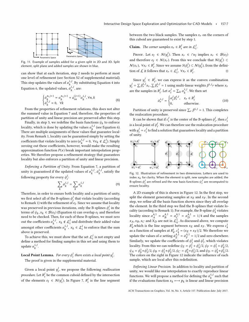
Fig. 12. Illustration of refinement in two dimensions. Letters are used toindex xk for clarity. When the element is split, new samples are added, theB-splines ϕ ji are refined and the new basis functions ψ j

i are recomputed toensure locality.

A 2D example of this is shown in Figure 12. In the first step, we

split the element generating samples at xE and xF . In the second

step, we refine all the basis function shown since they all overlap

the element. In the third step we find the B-splines that violate lo-

cality (according to Remark 1). For example, the B-spline ϕ1

4violates

locality since α4,1A = α4,1

B = α4,1C = α4,1

D = 1/4 and the samples

xA,xB ,xC and XD are not in L1

4. As discussed above, we compute

R1

4,which is the line segment between xE and xF . We express c1

4

as a function of samples at R1

4, c1

4= (xE + xF )/2. We therefore we

update the values of α setting α4,1E = α4,1

F = 1/2 and zero elsewhere.

Similarly, we update the coefficients of ϕ1

1and ϕ1

7, which violates

locality. From this we can redefineψE = ϕ1

1+ϕ1

4/2,ψF = ϕ

1

7+ϕ1

4/2,

ψA = ϕ1

0+ϕ1

3/2,ψB = ϕ

1

2+ϕ1

5/2,ψC = ϕ

6

0+ϕ1

3/2, andψD = ϕ

1

8+ϕ1

5/2.

The colors on the right in Figure 12 indicate the influence of each

sample, which are local after this redefinition.

Enforcing Linear Precision. In addition to locality and partition of

unity, we would like our interpolation to exactly reproduce linear

functions. We will propose a method for defining the αi, jk such that

if the evaluations function xk 7−→ pk is linear and linear precision



was enforced in all previous iterations, then∑k

αi, jk pk =

∑k

αi, jk pk (11)

From Equation 7, this implies that, in the linear case, the approxi-

mation does not change with refinement and therefore continues to

exactly reproduces linear functions after each iteration.

For intuition, let us first consider the special case when αji =∑

k αi, jk = 1. Under this assumption, the realocation procedure with

yji = c

ji results in c

ji =

∑k α

i, jk xk , since α

i, jr = β

i, jr , ∀xr ∈ R

ji .

Let pc jibe the evaluation at c

ji . If the evaluation function is linear,

then above expression yields pc ji=

∑k α

i, jk pk . On the other hand,

If linear precision was guaranteed in all previous iterations, then

pc ji= P(c

ji ). Since every B-spline evaluates to 1 on its center and

partition of unity is guaranteed, Equation 7 yields P(cji ) =

∑k α

i, jk pk .

From this we conclude that Equation 11 holds and therefore linear

precision is preserved.

Unfortunately, in general, we cannot guarantee that αji = 1. While

this was true in the example in Figure 12, this is usually not the case

in high dimensions and after multiple iterations. Our solution there-

fore is to use the realocation procedure with yji =

∑k α

i, jk xk/α

ji

(notice that when

∑k α

i, jk = 1, y

ji = c

ji ). This is possible because

we can prove that for this definition of yji , S(ϕ

ji ) ⊂ N(y

ji ) (supple-

mental material). By directly following the sequence of arguments

above, we can show that, for this definition of yji , linear precision is

guaranteed in the general case.

ALGORITHM 1: Refine (el ) along direction d

// Step 1 (Element Refinement)

create child nodes eiA and eiB ;create new samples on corners of every common cuboid;

// Step 2 (Basis Refinement)

forall ϕ ji which overlaps el doif S (ϕ ji (x )) larger than el along direction d then

// refine ϕ jiforall k, xk ∈ L

ji do

αn, j+1

k = αn, j+1

k + a(j+1)

in α i, jk , ∀n;α i, jk = 0;

endend

end// Step 3 (Combination)

forall ϕ ji which overlaps el doif ϕ ji violates locality then

set y ji =∑k α

i, jk xk /(

∑k α

i, jk );

set R ji = ∩el , ∀el ∈ N(y ji );compute β i, jr such that y ji =

∑β i, jr xr , xr ∈ R ji ;

compute the updated values of α , α :

α i, jr =(∑

k αi, jk

)β i, jr , xr ∈ R ji

α i, jr = 0, otherwise

endend

5.3 Extension to Cubic B-splinesTo extend our method to cubic B-splines, we first redefine locality.

On a uniform grid, cubic B-splines generate smooth interpolations

by introducing dependencies on adjacent samples. We therefore de-

fine the neighborhood N(xk ) of a sample xk as the set of elements

that either contain the sample xk or are adjacent to some element

that contains the sample xk . Analogously, we define the neighbor-

hood B(el ) of an element el as the set of samples on its boundary

and on the boundaries of its adjacent elements (see Figure 13).

Fig. 13. The neighborhood N(xk ) of a sample xk (left) and the neighbor-hood B(el ) of an element el (right) for cubic B-splines.

As in the linear case, we say that an approximation preserves

locality if ∀k, S(ψk ) ∈ N (xk ); or, equivalently, if, for each element el ,any sample xk whose associated basis functionψk does not vanish

on el is contained in the neighborhoodB(el ) of that element. We use

the same method described in Algorithm 1, refining cubic B-splies

in step 2 if their support is larger than twice the size of the refined

element el in direction d . We use following refinement relation for

cubic B-splines (see Figure 14):

ϕ(j)i (x) = 1

8ϕ(j+1)

(2i−2)(x) + 1

2ϕ(j+1)

(2i−1)(x) + 6

8ϕ(j+1)

(2i) (x)

+ 1

2ϕ(j+1)

(2i+1)(x) + 1

8ϕ(j+1)

(2i+2)(x).

(12)

0

00

11

01

21

11

41

21

11

3

Fig. 14. Refinement of cubic B-splines.

To compute the approximation P l (x) at x ∈ el , we need the

meshes from all samples xk ∈ B(el ) to be represented in the canon-

ical format of el . If xk ∈ B(el ) \ B(el ), then xk ∈ B(el ), where el is

adjacent to el . Let xk be a sample in B(el ) ∩ B(el ) (see Figure 15).

Since plkand pl

kare stored during our pre-computational phase and

have the same geometry, we can compute a mapping F : plk→ pl

k

using barycentric coordinates and then apply it to plk to obtain plk .Locality ensures that this mapping only has to be done once for

each sample guaranteeing that errors do not accumulate.

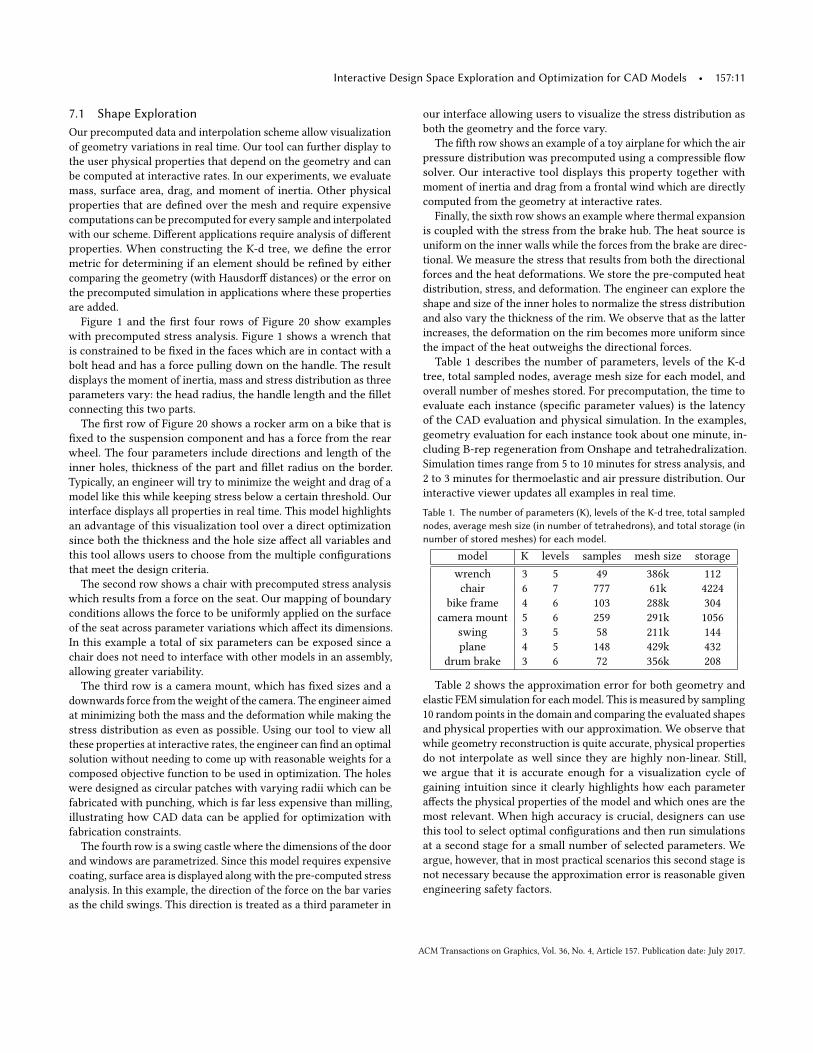
6 HOMEOMORPHIC MAPPINGIn this section we discuss how we define a homeomorphic map that

allows for representing a mesh pA in the canonical format of a given

element, pl . The resulting mesh plA should have the same geometry

as pA and the same combinatorics as the canonical reference pl (see



le le

l

kp

l

kp

kxk

x

Fig. 15. The mapping F : plk→ pl

kis used to obtain plk for xk ∈ B(el ) \

B(el ).

Figure 19). To this end, we need to establish a dense correspondence

between two meshes. Surface correspondence on meshes has been

extensively studied in previous work [Van Kaick et al. 2011]. Our

problem is distinct because we can take advantage of the CAD

referencing methods to establish partial correspondence. As we will

show in this section, this correspondence is not necessarily complete

since the topology of the internal CAD representations (B-rep) may

differ even if the geometry varies smoothly. We therefore propose

an algorithm that combines CAD data analysis with mesh surface

correspondence algorithms from previous work.

6.1 MotivationAs previously discussed, CAD systems use B-reps to represent solid

models, which are generated by computing a list of features. A

referencing scheme is used to determine the parts of the model

to which features are applied, allowing these to be correctly re-

generated if the model is modified. It is very common that parameter

changes affect the topology of the B-rep, even in cases in which

the geometry varies smoothly. Because references depend on the

feature history, not the B-rep itself, they are robust to topological

changes that do not affect the referenced element. An example of

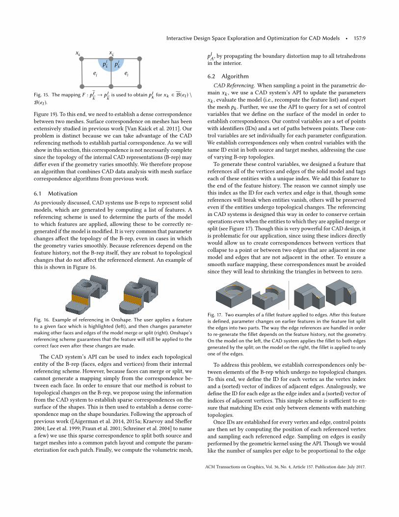
this is shown in Figure 16.

Fig. 16. Example of referencing in Onshape. The user applies a featureto a given face which is highlighted (left), and then changes parametermaking other faces and edges of the model merge or split (right). Onshape’sreferencing scheme guarantees that the feature will still be applied to thecorrect face even after these changes are made.

The CAD system’s API can be used to index each topological

entity of the B-rep (faces, edges and vertices) from their internal

referencing scheme. However, because faces can merge or split, we

cannot generate a mapping simply from the correspondence be-

tween each face. In order to ensure that our method is robust to

topological changes on the B-rep, we propose using the information

from the CAD system to establish sparse correspondences on the

surface of the shapes. This is then used to establish a dense corre-

spondence map on the shape boundaries. Following the approach of

previous work ([Aigerman et al. 2014, 2015a; Kraevoy and Sheffer

2004; Lee et al. 1999; Praun et al. 2001; Schreiner et al. 2004] to name

a few) we use this sparse correspondence to split both source and

target meshes into a common patch layout and compute the param-

eterization for each patch. Finally, we compute the volumetric mesh,

plA, by propagating the boundary distortion map to all tetrahedrons

in the interior.

6.2 AlgorithmCAD Referencing. When sampling a point in the parametric do-

main xk , we use a CAD system’s API to update the parameters

xk , evaluate the model (i.e., recompute the feature list) and export

the mesh pk . Further, we use the API to query for a set of control

variables that we define on the surface of the model in order to

establish correspondences. Our control variables are a set of points

with identifiers (IDs) and a set of paths between points. These con-

trol variables are set individually for each parameter configuration.

We establish correspondences only when control variables with the

same ID exist in both source and target meshes, addressing the case

of varying B-rep topologies.

To generate these control variables, we designed a feature that

references all of the vertices and edges of the solid model and tags

each of these entities with a unique index. We add this feature to

the end of the feature history. The reason we cannot simply use

this index as the ID for each vertex and edge is that, though some

references will break when entities vanish, others will be preserved

even if the entities undergo topological changes. The referencing

in CAD systems is designed this way in order to conserve certain

operations evenwhen the entities towhich they are appliedmerge or

split (see Figure 17). Though this is very powerful for CAD design, it

is problematic for our application, since using these indices directly

would allow us to create correspondences between vertices that

collapse to a point or between two edges that are adjacent in one

model and edges that are not adjacent in the other. To ensure a

smooth surface mapping, these correspondences must be avoided

since they will lead to shrinking the triangles in between to zero.

Fig. 17. Two examples of a fillet feature applied to edges. After this featureis defined, parameter changes on earlier features in the feature list splitthe edges into two parts. The way the edge references are handled in orderto re-generate the fillet depends on the feature history, not the geometry.On the model on the left, the CAD system applies the fillet to both edgesgenerated by the split; on the model on the right, the fillet is applied to onlyone of the edges.

To address this problem, we establish correspondences only be-

tween elements of the B-rep which undergo no topological changes.

To this end, we define the ID for each vertex as the vertex index

and a (sorted) vector of indices of adjacent edges. Analogously, we

define the ID for each edge as the edge index and a (sorted) vector of

indices of adjacent vertices. This simple scheme is sufficient to en-

sure that matching IDs exist only between elements with matching

topologies.

Once IDs are established for every vertex and edge, control points

are then set by computing the position of each referenced vertex

and sampling each referenced edge. Sampling on edges is easily

performed by the geometric kernel using the API. Though we would

like the number of samples per edge to be proportional to the edge



length, we require similar sampling on source and target meshes

in order to establish correspondences. Since edge sizes can vary

significantly when parameters are changed, we sample each edge by

hierarchical subdivision until the length of each segment is smaller

than a given threshold, and generate IDs for each sample according

to this subdivision. In addition to the control points, our API call

also returns a list of paths that connect pairs of points that are

consecutive along an edge.

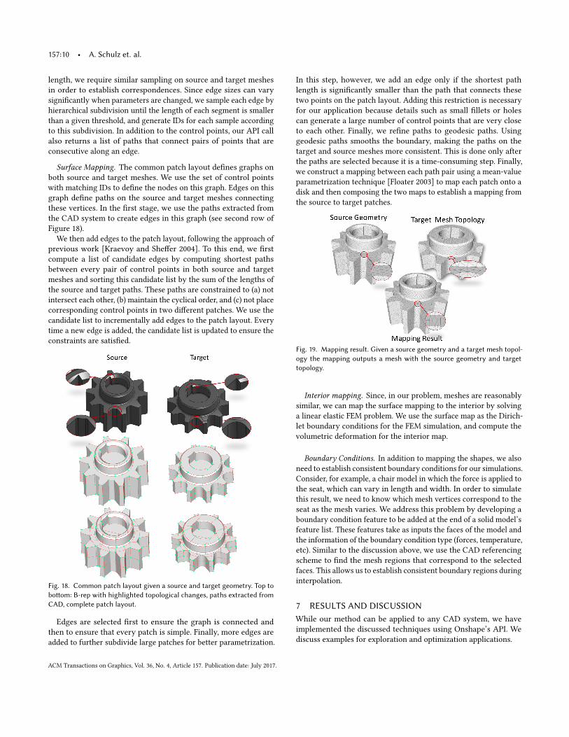
Surface Mapping. The common patch layout defines graphs on

both source and target meshes. We use the set of control points

with matching IDs to define the nodes on this graph. Edges on this

graph define paths on the source and target meshes connecting

these vertices. In the first stage, we use the paths extracted from

the CAD system to create edges in this graph (see second row of

Figure 18).

We then add edges to the patch layout, following the approach of

previous work [Kraevoy and Sheffer 2004]. To this end, we first

compute a list of candidate edges by computing shortest paths

between every pair of control points in both source and target

meshes and sorting this candidate list by the sum of the lengths of

the source and target paths. These paths are constrained to (a) not

intersect each other, (b) maintain the cyclical order, and (c) not place

corresponding control points in two different patches. We use the

candidate list to incrementally add edges to the patch layout. Every

time a new edge is added, the candidate list is updated to ensure the

constraints are satisfied.

Fig. 18. Common patch layout given a source and target geometry. Top tobottom: B-rep with highlighted topological changes, paths extracted fromCAD, complete patch layout.

Edges are selected first to ensure the graph is connected and

then to ensure that every patch is simple. Finally, more edges are

added to further subdivide large patches for better parametrization.

In this step, however, we add an edge only if the shortest path

length is significantly smaller than the path that connects these

two points on the patch layout. Adding this restriction is necessary

for our application because details such as small fillets or holes

can generate a large number of control points that are very close

to each other. Finally, we refine paths to geodesic paths. Using

geodesic paths smooths the boundary, making the paths on the

target and source meshes more consistent. This is done only after

the paths are selected because it is a time-consuming step. Finally,

we construct a mapping between each path pair using a mean-value

parametrization technique [Floater 2003] to map each patch onto a

disk and then composing the two maps to establish a mapping from

the source to target patches.

Fig. 19. Mapping result. Given a source geometry and a target mesh topol-ogy the mapping outputs a mesh with the source geometry and targettopology.

Interior mapping. Since, in our problem, meshes are reasonably

similar, we can map the surface mapping to the interior by solving

a linear elastic FEM problem. We use the surface map as the Dirich-

let boundary conditions for the FEM simulation, and compute the

volumetric deformation for the interior map.

Boundary Conditions. In addition to mapping the shapes, we also

need to establish consistent boundary conditions for our simulations.

Consider, for example, a chair model in which the force is applied to

the seat, which can vary in length and width. In order to simulate

this result, we need to know which mesh vertices correspond to the

seat as the mesh varies. We address this problem by developing a

boundary condition feature to be added at the end of a solid model’s

feature list. These features take as inputs the faces of the model and

the information of the boundary condition type (forces, temperature,

etc). Similar to the discussion above, we use the CAD referencing

scheme to find the mesh regions that correspond to the selected

faces. This allows us to establish consistent boundary regions during

interpolation.

7 RESULTS AND DISCUSSIONWhile our method can be applied to any CAD system, we have

implemented the discussed techniques using Onshape’s API. We

discuss examples for exploration and optimization applications.



7.1 Shape ExplorationOur precomputed data and interpolation scheme allow visualization

of geometry variations in real time. Our tool can further display to

the user physical properties that depend on the geometry and can

be computed at interactive rates. In our experiments, we evaluate

mass, surface area, drag, and moment of inertia. Other physical

properties that are defined over the mesh and require expensive

computations can be precomputed for every sample and interpolated

with our scheme. Different applications require analysis of different

properties. When constructing the K-d tree, we define the error

metric for determining if an element should be refined by either

comparing the geometry (with Hausdorff distances) or the error on

the precomputed simulation in applications where these properties

are added.

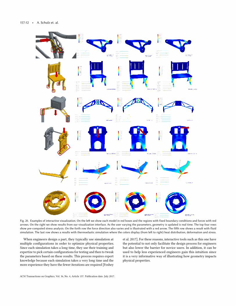
Figure 1 and the first four rows of Figure 20 show examples

with precomputed stress analysis. Figure 1 shows a wrench that

is constrained to be fixed in the faces which are in contact with a

bolt head and has a force pulling down on the handle. The result

displays the moment of inertia, mass and stress distribution as three

parameters vary: the head radius, the handle length and the fillet

connecting this two parts.

The first row of Figure 20 shows a rocker arm on a bike that is

fixed to the suspension component and has a force from the rear

wheel. The four parameters include directions and length of the

inner holes, thickness of the part and fillet radius on the border.

Typically, an engineer will try to minimize the weight and drag of a

model like this while keeping stress below a certain threshold. Our

interface displays all properties in real time. This model highlights

an advantage of this visualization tool over a direct optimization

since both the thickness and the hole size affect all variables and

this tool allows users to choose from the multiple configurations

that meet the design criteria.

The second row shows a chair with precomputed stress analysis

which results from a force on the seat. Our mapping of boundary

conditions allows the force to be uniformly applied on the surface

of the seat across parameter variations which affect its dimensions.

In this example a total of six parameters can be exposed since a

chair does not need to interface with other models in an assembly,

allowing greater variability.

The third row is a camera mount, which has fixed sizes and a

downwards force from theweight of the camera. The engineer aimed

at minimizing both the mass and the deformation while making the

stress distribution as even as possible. Using our tool to view all

these properties at interactive rates, the engineer can find an optimal

solution without needing to come up with reasonable weights for a

composed objective function to be used in optimization. The holes

were designed as circular patches with varying radii which can be

fabricated with punching, which is far less expensive than milling,

illustrating how CAD data can be applied for optimization with

fabrication constraints.

The fourth row is a swing castle where the dimensions of the door

and windows are parametrized. Since this model requires expensive

coating, surface area is displayed along with the pre-computed stress

analysis. In this example, the direction of the force on the bar varies

as the child swings. This direction is treated as a third parameter in

our interface allowing users to visualize the stress distribution as

both the geometry and the force vary.

The fifth row shows an example of a toy airplane for which the air

pressure distribution was precomputed using a compressible flow

solver. Our interactive tool displays this property together with

moment of inertia and drag from a frontal wind which are directly

computed from the geometry at interactive rates.

Finally, the sixth row shows an example where thermal expansion

is coupled with the stress from the brake hub. The heat source is

uniform on the inner walls while the forces from the brake are direc-

tional. We measure the stress that results from both the directional

forces and the heat deformations. We store the pre-computed heat

distribution, stress, and deformation. The engineer can explore the

shape and size of the inner holes to normalize the stress distribution

and also vary the thickness of the rim. We observe that as the latter

increases, the deformation on the rim becomes more uniform since

the impact of the heat outweighs the directional forces.

Table 1 describes the number of parameters, levels of the K-d

tree, total sampled nodes, average mesh size for each model, and

overall number of meshes stored. For precomputation, the time to

evaluate each instance (specific parameter values) is the latency

of the CAD evaluation and physical simulation. In the examples,

geometry evaluation for each instance took about one minute, in-

cluding B-rep regeneration from Onshape and tetrahedralization.

Simulation times range from 5 to 10 minutes for stress analysis, and

2 to 3 minutes for thermoelastic and air pressure distribution. Our

interactive viewer updates all examples in real time.

Table 1. The number of parameters (K), levels of the K-d tree, total samplednodes, average mesh size (in number of tetrahedrons), and total storage (innumber of stored meshes) for each model.

model K levels samples mesh size storage

wrench 3 5 49 386k 112

chair 6 7 777 61k 4224

bike frame 4 6 103 288k 304

camera mount 5 6 259 291k 1056

swing 3 5 58 211k 144

plane 4 5 148 429k 432

drum brake 3 6 72 356k 208

Table 2 shows the approximation error for both geometry and

elastic FEM simulation for eachmodel. This is measured by sampling

10 random points in the domain and comparing the evaluated shapes

and physical properties with our approximation. We observe that

while geometry reconstruction is quite accurate, physical properties

do not interpolate as well since they are highly non-linear. Still,

we argue that it is accurate enough for a visualization cycle of

gaining intuition since it clearly highlights how each parameter

affects the physical properties of the model and which ones are the

most relevant. When high accuracy is crucial, designers can use

this tool to select optimal configurations and then run simulations

at a second stage for a small number of selected parameters. We

argue, however, that in most practical scenarios this second stage is

not necessary because the approximation error is reasonable given

engineering safety factors.



Fig. 20. Examples of interactive visualization. On the left we show each model in red boxes and the regions with fixed boundary conditions and forces with redarrows. On the right we show results from our visualization interface. As the user varying the parameters, geometry is updated is real time. The top four rowsshow pre-computed stress analysis. On the forth row the force direction also varies and is illustrated with a red arrow. The fifth row shows a result with fluidsimulation. The last row shows a results with thermoelastic simulation where the colors display (from left to right) heat distribution, deformation and stress.

When engineers design a part, they typically use simulation at

multiple configurations in order to optimize physical properties.

Since each simulation takes a long time, they use their training and

expertize to pick certain configurations for testing and then to tweak

the parameters based on these results. This process requires expert

knowledge because each simulation takes a very long time and the

more experience they have the fewer iterations are required [Foshey

et al. 2017]. For these reasons, interactive tools such as this one have

the potential to not only facilitate the design process for engineers

but also lower the barrier for novice users. In addition, it can be

used to help less experienced engineers gain this intuition since

it is a very informative way of illustrating how geometry impacts

physical properties.



Table 2. Relative approximation error on geometry and elastic FEM for allexample models.

model

geometry geometry FEM FEM

max 99% max 99%

wrench 0.0028 0.0004 0.2138 0.0393

chair 0.0243 0.0022 0.3756 0.1130

bike frame 0.0112 0.0003 0.1403 0.0281

camera mount 0.0009 0.0002 0.4107 0.1861

swing 0.0013 0.0002 0.4750 0.2042

plane 0.0162 0.0055 - -

drum brake 0.0016 0.0006 0.3095 0.0490

7.2 Shape OptimizationWe also show how our method can be used for shape optimization.

For this application we use cubic B-splines, which guarantee smooth

interpolations. Using Equation 1, we can define the derivatives of

our approximation as

P ′(x) =∑k

pkψ′k (x), (13)

which can be expressed analytically sinceψk (x) is a sum of weighted

B-splines. We use this to drive a gradient-based algorithm for opti-

mization over objective functions defined on the mesh. We use an

interior point method and IpOpt for implementation.

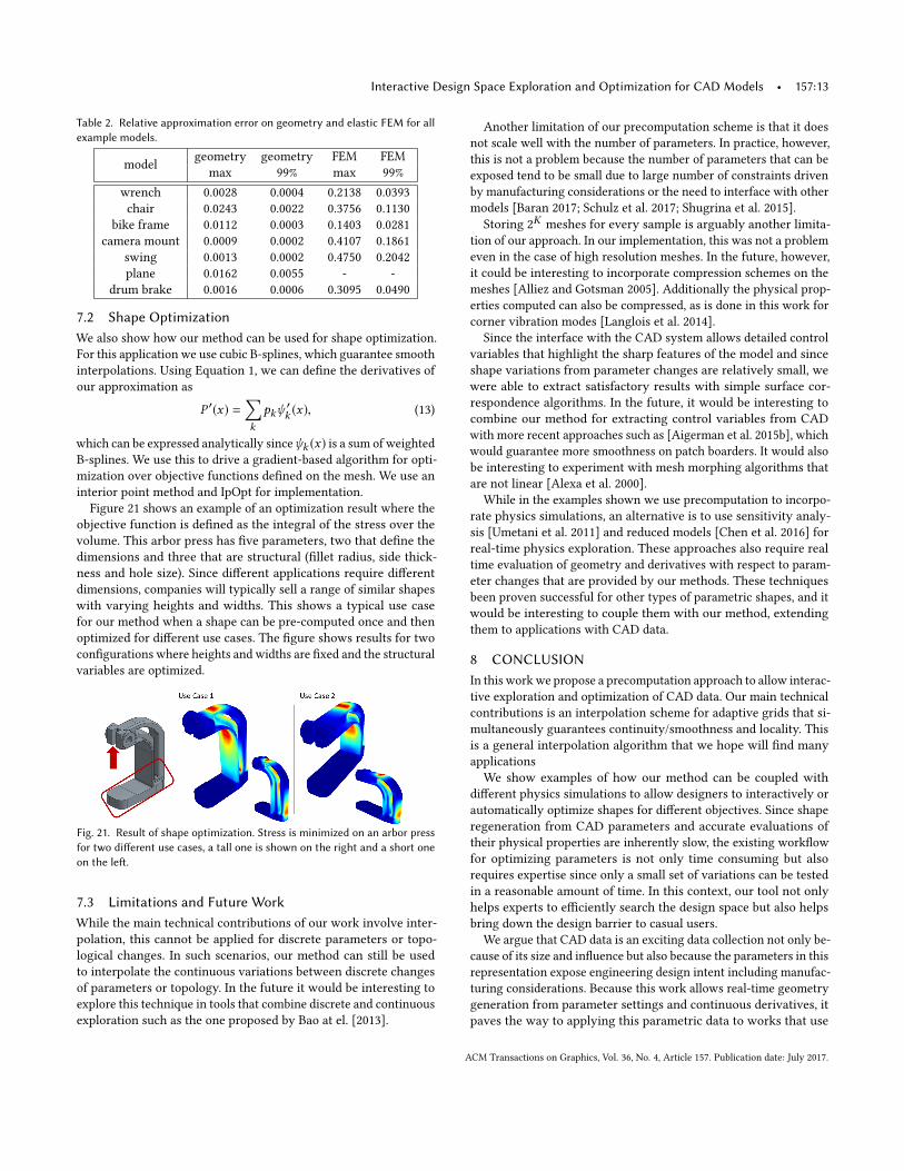
Figure 21 shows an example of an optimization result where the

objective function is defined as the integral of the stress over the

volume. This arbor press has five parameters, two that define the

dimensions and three that are structural (fillet radius, side thick-

ness and hole size). Since different applications require different

dimensions, companies will typically sell a range of similar shapes

with varying heights and widths. This shows a typical use case

for our method when a shape can be pre-computed once and then

optimized for different use cases. The figure shows results for two

configurations where heights and widths are fixed and the structural

variables are optimized.

Fig. 21. Result of shape optimization. Stress is minimized on an arbor pressfor two different use cases, a tall one is shown on the right and a short oneon the left.

7.3 Limitations and Future WorkWhile the main technical contributions of our work involve inter-

polation, this cannot be applied for discrete parameters or topo-

logical changes. In such scenarios, our method can still be used

to interpolate the continuous variations between discrete changes

of parameters or topology. In the future it would be interesting to

explore this technique in tools that combine discrete and continuous

exploration such as the one proposed by Bao at el. [2013].

Another limitation of our precomputation scheme is that it does

not scale well with the number of parameters. In practice, however,

this is not a problem because the number of parameters that can be

exposed tend to be small due to large number of constraints driven

by manufacturing considerations or the need to interface with other

models [Baran 2017; Schulz et al. 2017; Shugrina et al. 2015].

Storing 2Kmeshes for every sample is arguably another limita-

tion of our approach. In our implementation, this was not a problem

even in the case of high resolution meshes. In the future, however,

it could be interesting to incorporate compression schemes on the

meshes [Alliez and Gotsman 2005]. Additionally the physical prop-

erties computed can also be compressed, as is done in this work for

corner vibration modes [Langlois et al. 2014].

Since the interface with the CAD system allows detailed control

variables that highlight the sharp features of the model and since

shape variations from parameter changes are relatively small, we

were able to extract satisfactory results with simple surface cor-

respondence algorithms. In the future, it would be interesting to

combine our method for extracting control variables from CAD

with more recent approaches such as [Aigerman et al. 2015b], which

would guarantee more smoothness on patch boarders. It would also

be interesting to experiment with mesh morphing algorithms that

are not linear [Alexa et al. 2000].

While in the examples shown we use precomputation to incorpo-

rate physics simulations, an alternative is to use sensitivity analy-

sis [Umetani et al. 2011] and reduced models [Chen et al. 2016] for

real-time physics exploration. These approaches also require real

time evaluation of geometry and derivatives with respect to param-

eter changes that are provided by our methods. These techniques

been proven successful for other types of parametric shapes, and it

would be interesting to couple them with our method, extending

them to applications with CAD data.

8 CONCLUSIONIn this workwe propose a precomputation approach to allow interac-

tive exploration and optimization of CAD data. Our main technical

contributions is an interpolation scheme for adaptive grids that si-

multaneously guarantees continuity/smoothness and locality. This

is a general interpolation algorithm that we hope will find many

applications

We show examples of how our method can be coupled with

different physics simulations to allow designers to interactively or

automatically optimize shapes for different objectives. Since shape

regeneration from CAD parameters and accurate evaluations of

their physical properties are inherently slow, the existing workflow

for optimizing parameters is not only time consuming but also

requires expertise since only a small set of variations can be tested

in a reasonable amount of time. In this context, our tool not only

helps experts to efficiently search the design space but also helps

bring down the design barrier to casual users.

We argue that CAD data is an exciting data collection not only be-

cause of its size and influence but also because the parameters in this

representation expose engineering design intent including manufac-

turing considerations. Because this work allows real-time geometry

generation from parameter settings and continuous derivatives, it

paves the way to applying this parametric data to works that use



exploration and optimization of parametric shapes. We hope that

the techniques we present in this work will allow CAD data to be

applied to the plethora of the existing and upcoming research works

in the growing field of fabrication-oriented design.

ACKNOWLEDGMENTSThe authors would like to thank Ilya Baran for helpful sugges-

tions and discussions, Michael Foshey, Nicholas Bandiera and Javier

Ramos for discussions and for designing the models in the examples,

and the team at Onshape for support with the API.

REFERENCESAseem Agarwala. 2007. Efficient Gradient-domain Compositing Using Quadtrees. In

Siggraph 2007. ACM.

Noam Aigerman, Roi Poranne, and Yaron Lipman. 2014. Lifted bijections for low

distortion surface mappings. ACM Trans. Graph. 33, 4 (2014), 69.Noam Aigerman, Roi Poranne, and Yaron Lipman. 2015a. Seamless surface mappings.

ACM Trans. on Graph. (TOG) 34, 4 (2015), 72.Noam Aigerman, Roi Poranne, and Yaron Lipman. 2015b. Seamless Surface Mappings.

ACM Trans. Graph. 34, 4 (July 2015), 72:1–72:13.

Marc Alexa, Daniel Cohen-Or, and David Levin. 2000. As-rigid-as-possible shape

interpolation. In Siggraph 2000. ACM, 157–164.

Pierre Alliez and Craig Gotsman. 2005. Recent advances in compression of 3D meshes.

In Advances in multiresolution for geometric modelling. Springer, 3–26.Mehdi Baba-Ali, David Marcheix, and Xavier Skapin. 2009. A method to improve

matching process by shape characteristics in parametric systems. Computer-AidedDesign and Applications 6, 3 (2009), 341–350.

Moritz Bächer, Stelian Coros, and Bernhard Thomaszewski. 2015. LinkEdit: Interactive

Linkage Editing Using Symbolic Kinematics. ACM Trans. Graph. 34, 4 (July 2015),

99:1–99:8.

Fan Bao, Dong-Ming Yan, Niloy J. Mitra, and Peter Wonka. 2013. Generating and

Exploring Good Building Layouts. ACM Trans. Graph. 32, 4 (July 2013), 122:1–

122:10.

Ilya Baran. 2017. Onshape Inc. Personal Communication. (2017).

David Benson and Joel Davis. 2002. Octree textures. ACM Transactions on Graphics 21,3 (2002), 785–790.

Gaurav Bharaj, David I. W. Levin, James Tompkin, Yun Fei, Hanspeter Pfister, Wojciech

Matusik, and Changxi Zheng. 2015. Computational Design of Metallophone Contact

Sounds. ACM Trans. Graph. 34, 6 (Oct. 2015), 223:1–223:13.Rafael Bidarra and Willem F Bronsvoort. 2000. Semantic feature modelling. Computer-

Aided Design 32, 3 (2000), 201–225.

Rafael Bidarra, Paulos J Nyirenda, and Willem F Bronsvoort. 2005. A feature-based

solution to the persistent naming problem. Computer-Aided Design and Applications2, 1-4 (2005), 517–526.

Martin Bokeloh, Michael Wand, Hans-Peter Seidel, and Vladlen Koltun. 2012. An

Algebraic Model for Parameterized Shape Editing. ACM Trans. Graph. 31, 4 (July2012), 78:1–78:10.

Xiang Chen, Changxi Zheng, and Kun Zhou. 2016. Example-Based Subspace Stress

Analysis for Interactive Shape Design. IEEE Transactions on Visualization andComputer Graphics (2016).

Tao Du, Adriana Schulz, Bo Zhu, Bernd Bickel, and Wojciech Matusik. 2016. Computa-

tional Multicopter Design. ACM Trans. Graph. 35, 6 (Nov. 2016), 227:1–227:10.Gerald E Farin, Josef Hoschek, and Myung-Soo Kim. 2002. Handbook of computer aided

geometric design. Elsevier.Michael S Floater. 2003. Mean value coordinates. Computer aided geometric design 20, 1

(2003), 19–27.

Michael S Floater. 2015. Generalized barycentric coordinates and applications. ActaNumerica 24 (2015), 161–214.

David R. Forsey and Richard H. Bartels. 1988. Hierarchical B-spline Refinement. In

Siggraph 1988. ACM, 205–212.

Michael Foshey, Nicholas Bandiera, and Javier Ramos. 2017. Mechanical Engineers at

MIT. Personal Communication. (2017).

Eitan Grinspun, Petr Krysl, and Peter Schröder. 2002. CHARMS: A Simple Framework

for Adaptive Simulation. ACM Trans. Graph. 21, 3 (July 2002), 281–290.

Alec Jacobson, Ilya Baran, Jovan Popovic, and Olga Sorkine. 2011. Bounded biharmonic

weights for real-time deformation. ACM Trans. Graph. 30, 4 (2011), 78.Leif Kobbelt, Marc Stamminger, and Hans-Peter Seidel. 1997. Using Subdivision on

Hierarchical Data to Reconstruct Radiosity Distribution. Computer Graphics Forum(1997).

Yuki Koyama, Shinjiro Sueda, Emma Steinhardt, Takeo Igarashi, Ariel Shamir, and

Wojciech Matusik. 2015. AutoConnect: Computational Design of 3D-printable

Connectors. ACM Trans. Graph. 34, 6 (Oct. 2015), 231:1–231:11.

Vladislav Kraevoy and Alla Sheffer. 2004. Cross-parameterization and Compatible

Remeshing of 3D Models. In Siggraph 2004. ACM, 861–869.

Timothy R Langlois, Steven S An, Kelvin K Jin, and Doug L James. 2014. Eigenmode

compression for modal sound models. ACM Trans. Graph. 33, 4 (2014), 40.AaronWF Lee, David Dobkin, Wim Sweldens, and Peter Schröder. 1999. Multiresolution

mesh morphing. In Siggraph 1999. ACM, 343–350.

Seungyong Lee, GeorgeWolberg, and Sung Yong Shin. 1997. Scattered data interpolation

with multilevel B-splines. IEEE transactions on visualization and computer graphics3, 3 (1997), 228–244.

Frank Losasso, Frédéric Gibou, and Ron Fedkiw. 2004. Simulating Water and Smoke

with an Octree Data Structure. ACM Trans. Graph. 23, 3 (Aug. 2004), 457–462.Vittorio Megaro, Bernhard Thomaszewski, Maurizio Nitti, Otmar Hilliges, Markus

Gross, and Stelian Coros. 2015. Interactive Design of 3D-printable Robotic Creatures.

ACM Trans. Graph. 34, 6 (Oct. 2015).Przemyslaw Musialski, Thomas Auzinger, Michael Birsak, Michael Wimmer, and Leif

Kobbelt. 2015. Reduced-order Shape Optimization Using Offset Surfaces. ACMTrans. Graph. 34, 4 (July 2015).

PrzemyslawMusialski, Christian Hafner, Florian Rist, Michael Birsak, Michael Wimmer,

and Leif Kobbelt. 2016. Non-linear Shape Optimization Using Local Subspace

Projections. ACM Trans. Graph. 35, 4 (July 2016).

Emil Praun, Wim Sweldens, and Peter Schröder. 2001. Consistent mesh parameteriza-

tions. In Siggraph 2001. ACM, 179–184.

Romain Prévost, Emily Whiting, Sylvain Lefebvre, and Olga Sorkine-Hornung. 2013.

Make It Stand: Balancing Shapes for 3D Fabrication. ACM Trans. Graph. 32, 4 (July2013), 81:1–81:10.

John Schreiner, Arul Asirvatham, Emil Praun, and Hugues Hoppe. 2004. Inter-surface

mapping. In ACM Trans. Graph., Vol. 23. ACM.

Adriana Schulz, Ariel Shamir, Ilya Baran, David I. W. Levin, Pitchaya Sitthi-Amorn, and

Wojciech Matusik. 2017. Retrieval on Parametric Shape Collections. ACM Trans.Graph. 36, 1 (Jan. 2017), 11:1–11:14.

Adriana Schulz, Ariel Shamir, David I. W. Levin, Pitchaya Sitthi-amorn, and Wojciech

Matusik. 2014. Design and Fabrication by Example. ACM Trans. Graph. 33, 4 (July2014), 62:1–62:11.

Thomas W. Sederberg, Jianmin Zheng, Almaz Bakenov, and Ahmad Nasri. 2003. T-

splines and T-NURCCs. ACM Trans. Graph. 22, 3 (July 2003).

Rajsekhar Setaluri, Mridul Aanjaneya, Sean Bauer, and Eftychios Sifakis. 2014. SPGrid:

A Sparse Paged Grid Structure Applied to Adaptive Smoke Simulation. ACM Trans.Graph. 33, 6 (Nov. 2014).

Maria Shugrina, Ariel Shamir, and Wojciech Matusik. 2015. Fab Forms: Customizable

Objects for Fabrication with Validity and Geometry Caching. ACM Trans. Graph.34, 4 (July 2015), 100:1–100:12.

Mélina Skouras, Stelian Coros, Eitan Grinspun, and Bernhard Thomaszewski. 2015.

Interactive Surface Design with Interlocking Elements. ACM Trans. Graph. 34, 6(Oct. 2015).

Ian Stroud. 2006. Boundary representation modelling techniques. Springer Science &Business Media.

N Sukumar and EA Malsch. 2006. Recent advances in the construction of polygonal

finite element interpolants. Archives of Computational Methods in Engineering 13, 1

(2006), 129–163.

Nobuyuki Umetani, Takeo Igarashi, and Niloy J. Mitra. 2012. Guided Exploration of

Physically Valid Shapes for Furniture Design. ACM Trans. Graph. 31, 4 (2012).Nobuyuki Umetani, Danny M. Kaufman, Takeo Igarashi, and Eitan Grinspun. 2011.

Sensitive Couture for Interactive Garment Modeling and Editing. ACM Trans. Graph.30, 4 (July 2011), 90:1–90:12.

Nobuyuki Umetani, Yuki Koyama, Ryan Schmidt, and Takeo Igarashi. 2014. Pteromys:

Interactive Design and Optimization of Free-formed Free-flight Model Airplanes.

ACM Trans. Graph. 33, 4 (July 2014), 65:1–65:10.

Oliver Van Kaick, Hao Zhang, Ghassan Hamarneh, and Daniel Cohen-Or. 2011. A survey

on shape correspondence. InComputer Graphics Forum, Vol. 30.Wiley Online Library,

1681–1707.

Emily Whiting, Hijung Shin, Robert Wang, John Ochsendorf, and Frédo Durand. 2012.

Structural Optimization of 3D Masonry Buildings. ACM Trans. Graph. 31, 6 (2012),159:1–159:11.

Kun Xu, Yong Li, Tao Ju, Shi-Min Hu, and Tian-Qiang Liu. 2009. Efficient Affinity-based

Edit Propagation Using K-D Tree. In Siggraph Asia 2009. ACM, 118:1–118:6.

Youyi Zheng, Hongbo Fu, Daniel Cohen-Or, Oscar Kin-Chung Au, and Chiew-Lan Tai.

2011. Component-wise Controllers for Structure-Preserving Shape Manipulation.

In Computer Graphics Forum, Vol. 30. Wiley Online Library, 563–572.

Denis Zorin and Peter Schroder. 2000. Subdivision for Modeling and Animation. In

Siggraph 2000 Courses. ACM.


Documents

Interactive Design Space Exploration and Optimization … · shape space while geometry and physical ... Interactive Design Space Exploration and ... Interactive Design Space Exploration