Interactions in 4d Vasiliev theory:Locality, Unfolding and HolographyHigher Spin Theories Workshop, Penn State

Zhenya Skvortsov

Albert Einstein Institute and Lebedev Institute

August, 28, 2015

∗

∗Based on arxiv: 1508.04764 E.S. and M.Taronna; 1508.04139 also with P.Kessel and N.Boulanger and 1505.05887 P.Kessel, G.Lucena Gomez, E.S.,M.Taronna

Intro

A conjecture by Klebanov-Polyakov and Sezgin-Sundell relates4d Vasiliev HS theory to free/critical vector models.

There are remarkable tests of the 3-pt correlators by Giombiand Yin and of the one-loop effects by Beccaria, Bekaert,Giombi, Klebanov and Tseytlin.

In this talk we see how the interactions of HS fields look like asderived from the Vasiliev theory, explain some of the puzzlespreviously observed in HS AdS/CFT and put some new ones...

Approaches to the HS problem

via Fronsdal fields: individual cubic vertices (completecubic action in 3d and the 0-0-s part of the cubic actionin any d plus also 0-0-0-0 quartics in 4d).

Unfolded approach and Vasiliev’s equations: fullynonlinear equations of motion resumed into a relativelysimple system of equations.

To check the HS AdS/CFT duality, among other things, weneed to compute Witten diagrams that implicitly relies on thefact that we know how to relate the two approaches (e.g.boundary-to-bulk propagators for Fronsdal fields → HSconnections → unfolded HS interaction vertices →correlators).

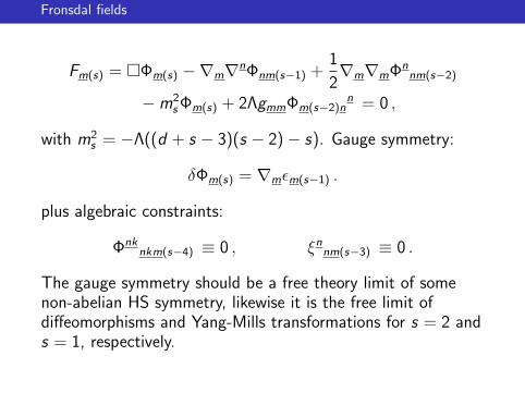
Fronsdal fields

Fm(s) = Φm(s) −∇m∇nΦnm(s−1) +1

2∇m∇mΦn

nm(s−2)

−m2s Φm(s) + 2ΛgmmΦm(s−2)n

n = 0 ,

with m2s = −Λ((d + s − 3)(s − 2)− s). Gauge symmetry:

δΦm(s) = ∇mεm(s−1) .

plus algebraic constraints:

Φnknkm(s−4) ≡ 0 , ξnnm(s−3) ≡ 0 .

The gauge symmetry should be a free theory limit of somenon-abelian HS symmetry, likewise it is the free limit ofdiffeomorphisms and Yang-Mills transformations for s = 2 ands = 1, respectively.

Unfolded equations

A nice first-order form any system can be put in

dWA = FA(W ) , FA(W ) =∑k

FAB1...BkWB1 ∧ ... ∧W Bk ,

Frobenius integrability implies

0 ≡ ddWA = dFA(W ) =⇒ FB ∧−→∂ FA(W )

∂W B ≡ 0 .

As a consequence of integrability, the unfolded equationspossess gauge symmetries

δWA = dξA + ξB−→∂ FA(W )

∂W B ,

The flatness condition dA = 12[A,A] is an example of an

unfolded system, the integrability = the Jacobi identity.

Unfolded field content

There are two fields in HS theory: a connection of the HSalgebra ω and a (twisted)-adjoint field C . The HS algebra isthe Weyl algebra in 4d thanks to so(3, 2) ∼ sp(4)

[qk , pj ] = iδkj ←→ [Y A, Y B ] = 2iCAB ,

with CAB being the sp(4) invariant tensor (charge conjugationmatrix). The bilinears deliver an oscillator realization of sp(4):

TAB = − i

4Y A, Y B , [TAB ,TCD ] = TADCBC + 3 more .

The HS algebra is the algebra of all (even) functions f (Y ) in

Y A. The product can be realized by the Moyal star-product:

(f ? g)(Y ) = f (Y ) exp i(←−∂ AC

AB−→∂ B

)g(Y ) ,

HS Unfolded equations

Unfolded equations for HS fields were searched in the form

dω = F ω(ω,C ) ,

dC = FC (ω,C ) ,

where the power of ω is fixed by the form degree and thestructure functions F ω,C admit an expansion in powers of thezero-form C

F ω(ω,C ) = V(ω, ω) + V(ω, ω,C ) + V(ω, ω,C ,C ) + ... ,

FC (ω,C ) = V(ω,C ) + V(ω,C ,C ) + V(ω,C ,C ,C ) + ... .

where ω = ωm(Y |x) dxm and C = C (Y |x)

Initial Vertices

The first vertices provide the initial data for the deformationproblem and are fixed by the HS algebra

V(ω, ω) = ω ? ω , V(ω,C ) = ω ? C − C ? π(ω) ,

where π flips AdS-translations, Pa → −Pa.

These vertices are consistent for any algebra. There areexamples of algebras (Vasiliev) that do not admit highervertices. The first highly nontrivial tests of HS AdS/CFT weredone by Giombi and Yin using V(ω,C ), which is the onlycontribution to 0− s1 − s2 in certain range of spins. Theone-loop tests (Beccaria, Giombi, Klebanov, Tseytlin) requireinformation about the free spectrum. Vertex V(ω,C ,C )revealed some puzzles...

Vacuum

dω = F ω(ω,C ) , dC = FC (ω,C ) .

Any flat connection ω = Ω is a solution at C = 0.

dΩ = Ω ? Ω ,

Anti-de Sitter space is a particular choice:

Ω =1

2$ααLαα + hααPαα +

1

2$ααLαα ,

where we split the sp(4) generators TAB into Lorentzgenerators Lαα = Tαα and Lαα = Tαα of sl(2,C)R andtranslation generators Pαα = Tαα with YA = (yα, yα).

Unfolded equations are naturally an expansion over a genericflat connection of the HS algebra, the deviation from beingflat are due C .

Free fields: linearized equation

When expanded over Ω we get to the lowest order

dω = Ω, ω? + V(Ω,Ω,C ) ,

dC = Ω ? C − C ? π(Ω) .

This set of equations contains the Fronsdal equations andexpresses other fields as derivatives of the Fronsdal field (ofunbounded order). Also there is Klein-Gordon equation hiddenin the second one for the scalar field of the HS multiplet.

ω =∑m,n

ωα(m),α(n)yα...yαyα...yα

C =∑m,n

Cα(m),α(n)yα...yαyα...yα

ω and C map

dotted (y)

undotted (y)

one-forms, ω

zero-forms, C

ωα(s−1),α(s−1)

Φm(s)

C α(2s)ωα(2s−2)

Cα(2s)

ωα(2s−2)V(Ω,Ω,C )

HS connection ω

At the free level the Fronsdal field is embedded as

Φm(s) = ωα(s−1),α(s−1)m hm|αα...hm|αα ,

while the rest are non-gauge invariant derivatives:

ωα(s−1∓k),α(s−1±k) : ∇b1 ...∇bk Φa1...as , k = 0, ..., s − 1 .

the derivatives are in the form of curls.

The last equations for ω define the HS Weyl tensor

∇b...∇bΦa(s) = C a(s),b(s)

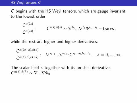
HS Weyl tensors C

C begins with the HS Weyl tensors, which are gauge invariantto the lowest order

Cα(2s)

C α(2s): C a(s),b(s) ∼ ∇b1 ...∇bs Φa1...as − traces ,

while the rest are higher and higher derivatives:

Cα(2s+k),α(k)

Cα(k),α(2s+k): ∇as+1 ...∇as+kC a1...as ,b1...bs , k = 0, ...,∞ .

The scalar field is together with its on-shell derivativesCα(k),α(k) ∼ ∇...∇Φ0

Free equations

Free equations can be summarized as

Dω = V(Ω,Ω,C ) , δω = Dξ , DC = 0 , δC = 0 ,

where D and D are the background covariant derivatives.Using the star-product one finds

D• = d • −Ω ? • ± • ? Ω = ∇− hαα(yα∂α + yα∂α) ,

D• = d • −Ω ? • ± • ? π(Ω) = ∇+ ihαα(yαyα − ∂α∂α) ,

∇ = d −$ααyα∂α −$ααyα∂α .

The vertex that glues C to the ω-equations reads:

V(Ω,Ω,C ) = −12Hαα∂α∂αC (y , y = 0)− 1

2H αα∂α∂αC (y = 0, y) ,

where Hαα = hαν ∧ hαν

Second order ↔ Cubic action

At the second order in the unfolded picture we find

Dω(2) − V(Ω,Ω,C (2)) = ω ? ω + V(Ω, ω,C ) + V(Ω,Ω,C ,C ) ,

DC (2) = ω ? C − C ? π(ω) + V(Ω,C ,C ) .

The free parts are on the left and the sources are on the right.There are vertices not determined directly by the HS algebra.

In the Fronsdal picture we expect to see (according toMetsaev’s classification there should not be more than∇s+s1+s2 derivatives on the r.h.s. in total)

Φ(2)s + ... = g

∑s1,s2

as,s1,s2∇...∇Φs1∇...∇Φs2 ,

where as,s1,s2 are fixed by the deformed HS symmetry. Theequations are supposed to come from an action

S = 12

∑s

∫ [(∇Φs)2 + . . .

]+

g

3

∑s,s1,s2

bs,s1,s2

∫(∇...∇Φs1∇...∇Φs2Φs)

Vasiliev equations: kinematics

We need to find all the vertices V(ω, ...,C ) that are notdetermined directly by the HS algebra. The unfolded equationsfor HS fields are folded into the Vasiliev generating equations.

The idea is that all V(ω, ...,C ) can be embedded into a flatconnection but of a bigger algebra:

(f ?g)(Y ,Z ) =

∫dUdVf (Y+U ,Z+U)g(Y+V ,Z−V )e iUAV

A

.

This gives back the usual ?-product on Z -independentfunctions, while [F (Y ), g(Z )]? = 0. In math it is a particularcase of the twisted product of noncommutative algebras.

The field content of the theory is given by one-form connectionW = Wm(Y ,Z |x) dxm, an auxiliary field SA = SA(Y ,Z |x)that is an sp(4)-vector and a zero-form Φ = Φ(Y ,Z |x).

Vasiliev equations: dynamics

The equations in sp(4)-covariant form read:

dW = W ?W ,

d(Φ ? κ) = [W ,Φ ? κ]? ,

dSA = [W , SA]? ,

[SA, SB ]? = −2i(CAB + Φ ? ΥAB) ,

SA ? Φ + Φ ? (Υ ? S ? Υ−1)A = 0 ,

where one needs a compensator VAB via Π±AB = 12(CAB ± VAB)

ΥAB =

(εαβe

iθκ 00 εαβe

−iθκ

)= Π+

ABeiθκ + Π−ABe

−iθκ ,

where there are a free parameter θ and two Klein operators

κ = e izαyα

, κ = e i zαyα

.

Extracting unfolded equations

Next step is to expand over a special vacuum W = AdS ,S = ZCdZ

C + A, Φ = 0 + B

∂A = A ? A + B ? Υ

∂B = A ? B − B ? Υ−1 ? A ? Υ

∂W = −[h + W ,A]

where ∂ = dZA∂ZA , A = ACdZC and h is a vielbein. One can

solve for the Z -dependence (in the Schwinger-Fock gaugeZCAC = 0)

A = ∂−1(A ? A + B ? Υ)

B = C (Y ) + ∂−1(A ? B − B ? Υ−1 ? A ? Υ)

W = ω(Y )− ∂−1[h + W ,A]

where C (Y ), ω(Y ) are the physical fields we are looking forequations for.

Extracting unfolded equations

The solutions for the Z -evolution need to be plugged into thetwo first equations

DW = W ?W + Lorentz , DB = W ? B − B ? W

to extract the equations in terms of C (Y ) and ω(Y ). There isalso an additional piece due to the requirement for the trueLorentz generators to preserve the Schwinger-Fock gauge,otherwise the spin-connection will appear outside the covariantderivative, which, for example, makes it difficult to relate HSvielbeins to Fronsdal fields. Lorentz redefinition contributes tothe stress-tensors.

Interaction Vertices: Rough structure

The rough structure of the vertices V(ω, ...,C ) is that onedoes three operations in many different ways. The operationsare: to compute the star-product of two fields, e.g.

C ? C

to add one, two homotopy integrals, which originate from ∂−1,

∂νfν = g(z) fα = zα

∫ 1

0

dt t g(zt)

to act with simple differential operators, e.g.

[h, zνfν(y , z)]∣∣∣z=0

= −ihνα∂yαfν(y , 0)

Therefore the vertices are ’very close’ to pure star-products

Second-order: V(h, h,C ,C )

Dω(2) − V(Ω,Ω,C (2)) = ω ? ω + V(Ω, ω,C ) + V(Ω,Ω,C ,C ) ,

DC (2) = ω ? C − C ? π(ω) + V(Ω,C ,C ) .

It is convenient to use Fourier transformed fields

C (y , y |x) =

∫d4ξ e iY ξC (ξ|x) .

and for the most complicated vertex V(h, h,C ,C )

V(h, h,C ,C ) =

∫d2ξ d2ηHααJαα(Y , ξ, η)C (ξ|x)C (η|x) + h.c . ,

where Hαα = hαβ ∧ hαβ is a basis two-form. All theinformation is hidden inside Jαα(Y , ξ, η).

Second-order summary

The most complicated vertex V(h, h,C ,C ) still fits the slide

J =

∫ 1

0

dt

∫ 1

0

dq(Hαα(y + ξ)α(y + η)αQ1

(iq2t2 + (ξη)

qt(1− qt)

2

)− i

2H ααξαηαQ1 +

i

2(1− t)H ααξαηαP1 +

i

2H αα∂α∂αK0 + h.c .

)(the very first term is due to the Lorentz redefinition)

K = exp i(tηξ + (y − η)(y + ξ) + 2θ

)Q = exp i

(qt(y + η)(y + ξ) + (y − η)(y + ξ) + 2θ

)P = Q

∣∣∣q=1

Pure star-product C ? π(C ) would give instead

exp i((y + η)(y + ξ) + (y − η)(y + ξ)

)

Gauge-invariant stress-tensors

Dω(2) − V(Ω,Ω,C (2)) = ω ? ω + V(Ω, ω,C ) + V(Ω,Ω,C ,C ) ,

DC (2) = ω ? C − C ? π(ω) + V(Ω,C ,C ) .

There is a part of the vertices that is gauge invariant andD-closed by itself (vertices talk to each other via dd = 0 ingeneral):

Js.t. =

∫ 1

0dt dq

[Hαα(y + ξ)α(y + η)αQ1

(iq2t2 + (ξη)

qt(1− qt)

2

)+

− i

2H ααξαηα

(Q1 − (1− t)P1

)+ h.c .

],

DJs.t. ≈ 0 ,

This is a part that is pseudo-local, i.e. has an unbounded numberof derivatives via C ? C .

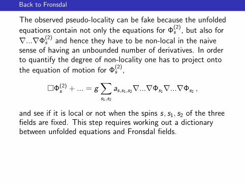
Back to Fronsdal

The observed pseudo-locality can be fake because the unfolded

equations contain not only the equations for Φ(2)s , but also for

∇...∇Φ(2)s and hence they have to be non-local in the naive

sense of having an unbounded number of derivatives. In orderto quantify the degree of non-locality one has to project onto

the equation of motion for Φ(2)s ,

Φ(2)s + ... = g

∑s1,s2

as,s1,s2∇...∇Φs1∇...∇Φs2 ,

and see if it is local or not when the spins s, s1, s2 of the threefields are fixed. This step requires working out a dictionarybetween unfolded equations and Fronsdal fields.

Back to Fronsdal: Solving for Torsion

The relevant part of the unfolded equations reads:

Dω(2) = J , DJ = 0 .

We need the first two equations: for HS vielbein e = ω0 andfirst HS spin-connection ω±1, where ωα(s−1±k),α(s−1∓k).

∇e + Q−ω1 = J0 ,

∇ω1 + Q−ω2 + Q+e = J1

where D = ∇+ Q− + Q+ = yαhαα ∂α + y αhαα ∂α.

The structure is similar to gravity with torsion

dea − ωa,b ∧ eb = T a ,

dωa,b − ωa,c ∧ ωc,b = Ja,b

Solving for Torsion: Fronsdal currents

HS equations in unfolded form always have a non-vanishingTorsion (solving for it destroys the beautiful structure):

ω1 = Q−1− (J0 −∇e)

Plugging it to the second equation and projecting outredundant components we find

Q+e −∇Q−1− ∇e = j j = (1−∇Q−1

− )J|1

The l.h.s. makes the Fronsdal operator. Assumption: Fronsdalfield at the second order can be identified with the samecomponent of ω:

Φm(s) = ωα(s−1),α(s−1)m hm|αα...hm|αα .

HS Weyl tensors

The equation for Weyl tensors is s curls of the Fronsdal one

(−m2W )∇m(s)Φn(s)|W = ∇m(s)jn(s)|W ,

However, C (2) does not equal to s-curls of Φ(2)

Dω(2) − V(Ω,Ω,C (2)) = R , DC (2) = P .

Instead there is an addon, which schematically is[∇sΦ(2) − C (2) = G R

]∣∣∣W,

where we define the resolvent G−1 = (I +∇Q−1− ). The

procedure is similar to solving for torsion but has to be iteratedto get to ωs−1 from ω0 ∼ Φ. A redefinition solves the problembut produces corrections to P. Comparing two legs of 0-0-swe see that the equations are not immediately Lagrangian.

Currents

Any current ∇njm(s−1)n = 0 can be decomposed as:

Current=nontrivial+improvement+e.o.m.

Restricting to scalars there is a standard current

j stdm(s) = Φ←→∇ m...

←→∇ mΦ + O(Λ) .

For every l > 0 there exist a conserved successor

j sucm(s) = ∇n(l)Φ←→∇ m...

←→∇ m∇n(l)Φ + O(Λ) .

There is a simple generating function for all these

j(y , y) =

(∂

∂uα∂

∂vα

∂

∂uα∂

∂vα

)l

C (u, u|x)C (−v , v |x)∣∣∣U=V=Y

.

Canonical sector

We cannot see the ’e.o.m.’ part since we are on-shell, but wesee some of the improvements evaluated on-shell and the latterwe can drop, which simplifies the expressions a lot. Moreover,improvements do not contribute to 3-p.t. correlators.

Jcan. =

∫ 1

0

dt

∫ 1

0

dq[1

4Hαα∂α∂αQ1

(i + (ξη)

(1− qt)

2qt

)+

i

8H αα∂α∂α

(Q1 − (1− t)P1

)+ h.c .

].

Corrections to Fronsdal equations

Restricting to the canonical sector and to the currents builtout of two scalar fields we find (the most general currents arealso available)

Φm(s) + ... = 2 cos 2θ∑l ,k

al ,k∇m(s−k)n(l)Φ∇m(k)n(l) Φ− tr ,

al ,k =(−)ks!s!

l !l !k!k!(s − k)!(s − k)!

s(2l(s − 1) + s(2s − 1))

8(s − 1)(l + s)2(l + s + 1)2

The large-l fall-off is improved by l−3 as compared to barestar-product C ? π(C ) which leads to (l !l !)−1. Theθ-dependence looks puzzling in view of the slightly-broken HSsymmetry.

Pseudo-local currents

Φm(s) + ... = 2 cos 2θ∑l ,k

al ,k∇m(s−k)n(l)Φ∇m(k)n(l) Φ ,

al ,k =(−)ks!s!

l !l !k!k!(s − k)!(s − k)!

s(2l(s − 1) + s(2s − 1))

8(s − 1)(l + s)2(l + s + 1)2

The Fronsdal currents are pseudo-local expressions, while weknow from the Lagrangian approach that the only nontrivialcoupling 0-0-s of two scalars with a HS field has s-derivatives.Therefore we are using an over-complete base of structures! Achain of redefinitions is needed to remove the improvementsreducing everything to the standard form.

Localizing pseudo-local couplings

We want to bring the Fronsdal currents into the standard formas to derive the couplings as,s1,s2 (compare with Bekaert et al.)

Φ(2)s + ... = g

∑s1,s2

as,s1,s2∇...∇Φs1∇...∇Φs2 ,

Several methods should give the same result for as,s1,s2

Integration by parts using free equations

Computation of an amplitude

Redefinition in the equations of motion

Coupling=nontrivial+Improvements, projection onto thenon-trivial part (representation theory)

Computation of an AdS/CFT correlation function(projects automatically)

Localizing pseudo-local couplings: toy model

It is known that the only scalar cubic vertex is a non-derivativeone, ’Φ3’, but suppose we are given

S =

∫1

2Φ(−m2)Φ +

1

2Ψ(−M2)Ψ− a0Φ2Ψ− a1(∂Φ)2Ψ + ...

The equations contain non-standard terms

(−M2)Ψ = a0Φ2 + a1(∂Φ)2 + ...

which can be redefined away using (Φ2) = 2m2Φ2 + 2(∂Φ)2

After redefinition we get the standard coupling we new a0

Ψ→ Ψ + 12a1Φ2 ,

a0 → a0 + 12a1(2m2 −M2) .

The same contribution is added to the 3-p.t. correlator〈OOO〉 ∼ a0 (Freedman et al, early years of AdS/CFT)

Localizing pseudo-local couplings: toy model

Given the most general source, the equations

Ψ =∑l

al∇m(l)Φ∇m(l)Φ

are seemingly well-defined for any al , but∑l

al

∫Ψ∇m(l)Φ∇m(l)Φ ∼

∑l

alCl

∫Ψ′Φ2

tells us that all the terms are proportional to each other, andthe question is whether a =

∑l alCl is convergent or not,

where Cl are the numbers produced by integrations by partsand commuting covariant derivatives. Other methods give thesame result.

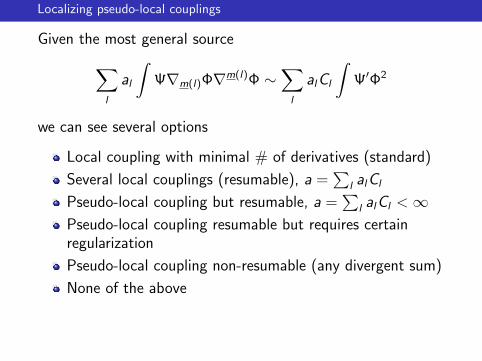
Localizing pseudo-local couplings

Given the most general source∑l

al

∫Ψ∇m(l)Φ∇m(l)Φ ∼

∑l

alCl

∫Ψ′Φ2

we can see several options

Local coupling with minimal # of derivatives (standard)

Several local couplings (resumable), a =∑

l alCl

Pseudo-local coupling but resumable, a =∑

l alCl <∞Pseudo-local coupling resumable but requires certainregularization

Pseudo-local coupling non-resumable (any divergent sum)

None of the above

Gaps in the bridge

What is the relation between HS connection and Fronsdalfields? Basic invariants

Φm(s) = tr(em ? ... ? em)

can be combined with the powers thereof (Campoleoni etal)

Φm(s) = Φm(s) +∑

n+m=s

bn,mΦm(n)Φm(m) + ...

Moreover, one can add a C -dependence, which makessuch identification pseudo-local.

Another subtle point is the choice of the gauge inVasiliev’s equations. Different gauges=different unfoldedequations for HS, that are related through (inadmissiblesometimes) field-redefinitions (W (Y ,Z |x) is flat).

Testing Fronsdal currents

Combining all results we observe for l large

3d : Cl ∼ l !l2s−1 al ∼1

l !l3

4d : Cl ∼ l !l !l2s al ∼1

l !l !l3

Therefore, the resumed couplings diverge, e.g. in 4d

s = 2 : a002 = − 1

12

∞∑n=1

l ,

s = 4 : a004 = − 1

3 · 7!

∞∑l=1

l(l + 1)(l + 2)2(3l + 11)(5l(l + 4) + 3)

(l + 3)(l + 4)

This result was anticipated in (Boulanger, Leclerc andSundell) and is in accordance with Giombi and Yin’s puzzles.Along the way we defined the functional class that does notlead to any problems for pseudo-local expressions.

Testing Fronsdal currents

This result can be anticipated noticing that the interactionvertices are very close to pure star-products, e.g.ω ? ω ? C ? π(C ). The trace-invariant of the HS algebra

tr(C (Y |x) ? π(C (Y |x)) ? ...) = ,

makes sense as a bulk object and computes all correlators ofthe free duals upon plugging b-to-b propagators(Colombo-Sundell; S.Didenko, E.S.). It can be expanded inHS Weyl tensors and derivatives, each term being local, but asa whole the trace does not depend on x at all!(C (Y |x) = g ?C (Y )?π(g−1), where g = g(Y |x)). Therefore,

tr(...) ∼∫AdS

∑alCl =∞

Analogous puzzle in 3d

The 3d case: Prokushkin-Vasiliev theory at the second order

Dω2 = J(C ,C ) , (−M2 + ...)Φs =∑l

al∇lφ←→∇ s∇lφ

DC2 = [ω,C ] , (−m2)φ = (∇)sφΦs

The Fronsdal equation produces a divergent series for thecoupling

∑Clal . However, it can be found from the scalar

field equation, which is local, to be related to the HS algebrastructure constants. Then one can compute the correlationfunction. The result agrees with the CFT. The puzzle is thatthe equations coming from the same Lagrangian vertex are notrelated in an obvious way.

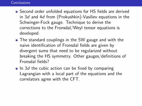
Conclusions

Second order unfolded equations for HS fields are derivedin 3d and 4d from (Prokushkin)-Vasiliev equations in theSchwinger-Fock gauge. Technique to derive thecorrections to the Fronsdal/Weyl tensor equations isdeveloped.

The standard couplings in the SW gauge and with thenaive identification of Fronsdal fields are given bydivergent sums that need to be regularized withoutbreaking the HS symmetry. Other gauges/definitions ofFronsdal fields?

In 3d the cubic action can be fixed by comparingLagrangian with a local part of the equations and thecorrelators agree with the CFT.