Embed Size (px)
Citation preview

Interaction between turbulent flow and saturated porous media
Mahesh Prakash
A thesis submitted in fulfillment of the requirements for the degree of Doctor of Philosophy
School of the Built Environment Victoria University
Melbourne, Australia
June 2000
T: o
LIBRARY g

FTS THESIS 532.052" PR.\ 30001006992236 Prakash, Mahesh Interaction between turbulent flow and saturated porous media

Declaration of candidate
This thesis contains no material that has been accepted at another university for the award of a degree, and to the best of the author's knowledge and belief, the thesis contains no material previously published by others, except where reference is made.
(Mahesh Prakash)
Melboume, Australia June, 2000

Abstract
In this thesis, the interaction between turbulent flow and saturated porous
media has been investigated using computational fluid dynamics (CFD) simulations,
flow visualisation experiments and laser Doppler velocimetry (LDV) measurements.
In these systems, turbulence in the fluid layer may persist in the adjacent porous
medium before it is attenuated at a rate that depends on the permeability and porosity
of the porous medium. Synthetic reticulated foam of different permeabilities has been
used as the porous medium for the experiments. Due the opaque nature of the porous
foam, visualisations and measurements have been carried out in the fluid layer. The
interaction between the turbulent fluid layer and the porous foam leads to changes in
the flow pattern in the fluid layer. These changes have been recorded through the
experiments for the purpose of evaluating the numerical model.
The flow visualisations have revealed that the permeability of the porous foam
and the height of the fluid layer above the porous foam significantiy affect the flow
pattern, at least in the fluid layer. The thickness of the porous foam affects the flow
pattem to a smaller extent. For low permeability porous foams, it has been found that
there is little change in the flow pattem in the fluid layer from the cases without foam.
It has been concluded that in such cases, the fluid layer and the porous medium can be
regarded to be operating in the turbulent and laminar regimes, respectively. In case of
the highest permeability foam tested, the flow pattem changes significantly in the
fluid layer, indicating a stiong interaction between the flow in the fluid layer and the
adjacent foam.
Three different models were used to represent the flow in the porous foam,
namely a laminar flow model and two turbulence models. The objective has been to
infer the effect of the presence or absence of macroscopic turbulence in the porous
medium by studying the changes in the flow pattem, mean velocities and turbulence
kinetic energy in the fluid layer. The reason for such an indirect evaluation is the
inability of using measurements made at point locations in the porous medium for
comparison with simulations using volume averaged equations.
Of the two turbulence models used in this study, one has only Darcy damping
in the turbulence tiansport equations for the porous foam. This model has been found
to be qualitatively superior in predicting the gross flow patterns. The second
11
turbulence model has Darcy and Forchheimer modifications included in the
turbulence transport equations for the foam. This model has been found to be
qualitatively similar to the laminar flow model in its predictive capabilities. The
reason for the similarity is the almost complete damping of turbulence at the interface
between the foam and clear fluid due to the Darcy and Forchheimer modification
terms. None of the three models used to represent flow in the foam can adequately
predict the effect of changes in the thickness of the porous layer.
In order to consolidate on the flow visualisations, LDV measurements have
been carried out for a quantitative comparison between the CFD simulations and the
measurements. The vector plots obtained from the measurements confirmed that
there is a significant change in the flow pattem in the fluid layer in the case of the
highest permeability foam investigated. It has been fiirther observed that the
numerical simulations predict the mean axial velocity profiles better with the first
turbulent flow model with only Darcy damping for the foam. For the radial velocity
profiles, predictions with the laminar flow model and the second turbulence model
with both Darcy and Forchheimer modification terms are better at the highest fluid
height in a region close to the interface between the fluid layer and foam. On the
other hand, the first turbulent flow model with Darcy damping gives results that are in
better agreement with the measurements for the radial velocity with a decrease in the
height of the fluid layer. The predicted turbulence kinetic energy profiles in the fluid
layer using any of the three models for the foam have relatively good agreement with
the experimental results.
After validating the numerical modelling of the interaction between a turbulent
fluid flow overlying a saturated porous layer with experimental results, the numerical
work has been extended to an industrially important case study concerning moisture
migration in respiring agricultural produce. In this case study, a general procedure
has been developed to simulate systems with a turbulent fluid layer overlying a
saturated hygroscopic porous medium. Such a model is capable of predicting the
moisture migration process more accurately than existing models, as it accounts for
turbulence in the fluid layer.
Ill

Acknowledgements
I would like to take this opportunity to thank my supervisors, Associate
Professor (jraham Thorpe, Associate Professor Ozden Turan and Dr. Yuguo Li who
have guided and supported me throughout the course of my doctoral research. I wish
to thank my postgraduate student colleagues who assisted me immensely, to make my
stay in Austialia as an overseas student, a very pleasant experience. Thanks are due
to the Head of the School of the Built Environment, Associate Professor Michael Sek,
for his words of wisdom and encouragement. 1 am grateful to the technical and
secretarial staff of the school and the university who provided me with all the help
needed, towards the successful completion of my doctoral research. I would like to
acknowledge the School of the Built Environment for providing me with a
departmental scholarship for pursuing my doctoral study in Austialia. I would also
like to acknowledge the Commonwealth Scientific and Industrial Research
Organisation (CSIRO), Australia for allowing me to use their experimental facilities.
Special thanks go to Mr. John Mahoney who provided me with technical assistance
while performing my experiments at CSIRO, Building Constmction and Engineering
in Highett, Victoria, Austialia.
I would like to dedicate this thesis to my parents in India who have throughout
been extremely encouraging and supportive.
IV
List of Symbols
aE, aw. ttN, as, ap coefficients associated with the final discretised equation avd dynamic specific surface area [m' ] b discretised source term c speed of light [ms'^j Cfi dimensionless coefficient in Vt, eddy viscosity. c^ new constant associated with the macroscopic k-e turbulence
model for flow through porous media Cei, Ce2, Ce3 Coefficients associated with the rate of dissipation of turbulence
kinetic energy Ca specif ic hea t o f air at cons tan t p ressure [Jkg"^°K"*] Cb bulk specific heat at constant pressure [Jkg"'°K"'] CF Forchheimer coefficient Cp, Cp specific heat at constant pressure [Jkg"'°K''] Cvv specific heat of liquid water at constant pressure [Jkg' °K' ] D inner diameter of the acrylic cylinder [m] D width of the system [m] Das rate coefficient for moisture exchange between air and porous
medium [s"'] Dj jet diameter [m] dp average pore diameter of the porous medium [m] ei, 62,1 unit vectors //, fi, f^l damping functions associated with the low Reynolds number k-
e turbulence model fh fii, fi2 frequencies of laser beams [Hz] fiD approximate frequency difference betweenyj/ and7/2 [Hz] g acceleration due to gravity [ms" ] H height of the fluid layer or height of the entire system [m] hp thickness of the porous foam [m] Hy, integral heat of wetting [Jkg"'] /, j , k counters K permeability [m^] K permeability tensor [m ] k turbulence kinetic energy [m s" ] kb thermal conductivity of the solid matrix [Wm' °K' ] kf thermal conductivity of the fluid [Wm'' °K'' ] n number of samples taken per point in LDV measurements p pressure [Pa] Patm atmospheric pressure [Pa] Psat saturation pressure [Pa] R inner radius of the acrylic cylinder [m] r, z axi-symmetric co-ordinates [m] Rf^ radius of the nozzle [m] T temperatiire [°K] t time [s] u velocity vector [ms' ] u, V velocities [ms' ] Ub bulk jet velocity [ms' ']
ix

Up pore velocity for flow through porous medium [ms"'] W moisture content of the porous medium on a dry basis [kg of
moisture/ kg of dry solid] w air moisture content on a dry basis [kg of moisture/ kg of dry
air] X, y cartesian co-ordinates [m] xu, yv staggered locations in the cartesian co-ordinate system [m]
Greek symbols
P coefficient of thermal expansion [°K''] p density [kgm"^] p dynamic viscosity of the fluid [Pas] V kinematic viscosity of the fluid [m^s"'] ri Kolmogorov length scale [m] ^ porosity of the porous medium e rate of dissipation of turbulence kinetic energy [m s" ] (p representative scalar variable T shear stiess [kgm" s' ] A symbol representing difference cr turbulent Prandtl number K von Karman's constant 5ij Kronecker's delta, 5ij = 1 for / =j and <% = 0 for i^j Pt absolute eddy or turbulent viscosity [Pas] Vt kinematic eddy or turbulent viscosity [m s' ]
Subscripts
pa phase averaged quantity va volume averaged quantity eff effective value /, j , k vector components or counters r, 6, z vector components in cylindrical co-ordinates w value associated with the wall imin, imax minimum and maximum values e, w, n, s east, west, north and south confrol surfaces around a grid point ref reference value avg average value
Superscripts
E,W,N,S east, west, north and south neighbours of a grid point c convective component d diffiisive component g guess value nd non-dimensional value

List of Tables
Table Tide Page No.
2.1 Examples of low Reynolds number turbulence models. 28
3.1 Accuracy of the solution for air at Ra^lO^, lO"* and 10^ 59
3.2 Accuracy of the solution for air at Ra= 10 . 60
3.3 Accuracy of the solution for air at Ra= 10 . 62
3.4 Effect of grid distribution on accuracy. 64
3.5 Summary of solutions for turbulent flow with Ra=5xl0^^. lA
A. 1 Stmctural parameters of synthetic foam investigated by
Seguine^a/. (1998a). 81
4.2 Permeability, K, and Forchheimer coefficient, Cf for foam. 81
6.1 Shift in the location of the measuring volume in case of the horizontal beam alignment (corresponding to the radial velocity measurements). 162
7.1 Grid refinement study for the simulations of the experiments of Kirkpatrick and Bohn (1986) using wall Nusselt numbers. 219
7.2 Coefficient of Nusselt number to Rayleigh number relationship. 220
XI

List of Figures
Figure Tide Page No.
2.1 Staggered locations for w. 30
2.2 Shaded area representing a scalar confrol volume. 31
2.3 Main and staggered grid locations for a 7x7 grid. 34
2.4 Representation ofthe line by line Gauss-Seidel method. 37
2.5 Control volume for the continuity equation. 39
2.6 Flow chart of the SIMPLE algorithm. 41
3.1 Square cavity that has vertical walls maintained at different temperatures, and the top and bottom walls are adiabatic. 46
3.2 Representative non-uniform mesh using a sine function for grid distribution in the x and y directions. 52
3.3 Numerical prediction ofthe flow field for increasing Rayleigh numbers for air in the laminar regime. 55-57
3.4 Variation in the (a) core stratification (b) average wall heat transfer with Rayleigh number for air in the laminar regime. 65
3.5 Variation of local wall heat fransfer for air at different Rayleigh
numbers in the laminar regime. 66
3.6 Nature ofthe solutions for turbulent flow {Ra = 5x10 ) for air. 69
3.7 Grid independence for turbulent flow. 73
3.8 Comparisonofwallheatfransfer for turbulent flow. Experimental results are from Cheesewright and co workers. 73
3.9 Further comparison between present numerical solutions and the experiments of Cheesewright and his co workers (a) vertical velocity, turbulent shear stiess, (c) turbulence kinetic energy, (d) eddy viscosity. 75-76
4.1 Schematic diagram ofthe irmer cylinder along with the impinging jet. 85
4.2 Schematic diagram ofthe experimental setup used for the impinging jet flow visualisations. 87
4.3 Preliminary flow visualisation results illustrating the central jet region and the effect of change in the exposure times. 88
Xll

4.4 (a) Actual image, (b) Enhanced image. //=0.15 m, Ap= 0 m, Ub= 1.6 m/s. 95
4.5 (a) Actual image, (b) Enhanced image. H=0.1 m, hp= 0 m, Ub=\.6 m/s. 95
4.6 (a) Actual image, (b) Enhanced image. i/=0.05 m, hp= 0 m, Ub=\.6 m/s. 96
4.7 (a) Actual image, (b) Enhanced image. H=0.15 m, hp= 0.05 m, i7i=1.6m/s, G60foam. 96
4.8 (a) Actual image, (b) Enhanced image. H^O. I m, hp= 0.05 m, CA=1.6 m/s, G60 foam. 97
4.9 (a) Actual image, (b) Enhanced image. H=0.05 m, ^p=0.05 m, (7^=1.6 m/s, G60 foam. 97
4.10 (a) Actual image, (b) Enhanced image. H=0.15 m, hp=0.05 m, ^4-1.6 m/s, G30 foam. 98
4.11 (a) Actual image, (b) Enhanced image. H=0.1 m, hp=0.05 m, C4=1.6 m/s, G30 foam. 99
4.12 (a) Actual image, (b) Enhanced image. i7=0.05 m, hp=0.05 m, t//,=1.6 m/s, G30 foam. 99
4.13 (a) Actual image, (b) Enhanced image. H=0.15 m, hp=0.1 m, (7/,= 1.6 m/s, G30 foam. 100
4.14 (a) Actual image, (b) Enhanced image. H=0.l m, hp=0.l m, £4=1.6 m/s, G30 foam. 101
4.15 (a) Actual image, (b) Enhanced image. H=0.05 m, hp=0.1 m, f4=1.6 m/s, G30 foam. 102
4.16 (a) Actual image, (b) Enhanced image. H=0.15 m, /zp=0.05 m, ^6=1.6 m/s, GIO foam. 103
4.17 (a) Actual image, (b) Enhanced image. H=0.1 m, hp=0.05 m, £4=1.6 m/s, GIO foam. 104
4.18 (a) Actual image, (b) Enhanced image. H=0.05 m, hp^0.05 m, £4=1.6 m/s, GIO foam. 104
4.19 (a) Actual image, (b) Enhanced image. H=0.15 m, hp=0.1 m, £4=1.6 m/s, GIO foam. 105
4.20 (a) Actual image, (b) Enhanced image. H=0.l m, hp=0.l m, £4=1.6 m/s, GIO foam. 106
4.21 (a) Actual image, (b) Enhanced image. H=0.05 m, hp=0.1 m, £4=1.6 m/s, GIO foam. 107
Xlll

4.22 Change in the radial position of the centre of re-circulation as a function of the fluid height for cases without foam. 108
4.23 Change in the radial position ofthe centre ofthe dominant re-circulation as a function of the fluid height for G10 foam with ^p=0.05 m. 108
5.1 Example of the non-uniform grid used for computations. H=0A5m,hp=0.0m. 125
5.2 Grid refinement study with //=0.15 m, hp=0.0 m, £4=1.6 m/s. 126
5.3 Example of the non-uniform grid used for computations. H=0A5m,hp=0.05m. 127
5.4 Grid refinement study with H=0.15 m, ^^=0.05 m, £4=1.6 m/s. 128
5.5 Stream traces and vector plots for cases without porous foam. 136
5.6 Turbulence kinetic energy contours for G10 foam with //=0.15m, hp=0.05 m, £4=1.6 m/s. (a) with FMB terms included in the k equation, (b) without FMB terms in the k equation. 137
5.7 Turbulence kinetic energy contours for (a) H=0.15 m, (b) H=0.1 m, (c) H=0.05 m with hp=0.05 m and £4=1.6 m/s. 138
5.8 Rate of energy dissipation contours for (a) H=0.15 m, (b) H=0.1 m, (c) H=0.05 m with hp=0.05 m and £7 = 1.6 m/s. 139
5.9 Eddy viscosity contours for (a) H=0.15 m, (b) H=0.1 m, (c) H=0.05 m with hp^0.05 m and £4= 1.6 m/s. 140
5.10 Stieam traces and vector plots for the cases with porous foam G45 with hp=O.OS m. Turbulence model TMl used for the porous foam. 141
5.11 Stieam tiaces and vector plots for the cases with porous foam G45 with hp=0.05 m. Turbulence model TM2 used for the porous foam. 142
5.12 Stieam traces and vector plots for the cases with porous foam G45 with hp=0.l m. Turbulence model TMl used for the porous foam. 143
5.13 Stieam tiaces and vector plots for the cases with porous foam G45 with hp=0.1 m. Turbulence model TM2 used for the porous foam. 144
5.14 Stieam traces and vector plots for the cases with porous foam GIO with hp=0.05 m. Turbulence model TMl used for the porous foam. 145
5.15 Stieam tiaces and vector plots for the cases with porous foam G10 with hp=0.05m. Turbulence model TM2 used for the porous foam. 146
5.16 Stieam tiaces and vector plots for cases with porous foam G10 with
xiv

Ap=0.1 m. Turbulence model TMl used for the porous foam. 147
5.17 Stream traces and vector plots for the cases with porous foam G10 with
hp=0.1 m. Turbulence model TM2 used for the porous foam. 148
6.1 An illustiation of the LDV operating in the fiinge mode. 152
6.2 Photograph ofthe experimental setup used for the LDV measurements. 154
6.3 Schematic diagram ofthe experimental setup used for the LDV measurements. 155
6.4 LDV measurements representing the magnitude of the uncertainty in the mean and r.m.s. velocities through repeatability tests. 157
6.5 LDV measurements indicating the deviation of the jet centre from the centre of the tank. 160
6.6 Horizontal beam analysis on centreline axis Y-Y. 161
6.7 Measurements and simulations for cases without foam. Vector plots and stream traces. 164
6.8 Change in the horizontal position ofthe centie of re-circulation as a function of the fluid height. 165
6.9 Axial velocity profiles for //=0.15 m, hp=0.0 m, £4= 1 -6 m/s. 168
6.10 Axial velocity profiles for .^=0.1 m, hp=0.0 m, £4= 1.6 m/s. 169
6.11 Axial velocity profiles for H=0.05 m, hp=0.0 m, £4= 1 -6 m/s. 170
6.12 Radial velocity profiles for H=0.15 m, hp-0.0 m, £4= 1.6 m/s. 171
6.13 Radial velocity profiles for H=0.1 m, hp=0.0 m, £4= 1.6 m/s. 172
6.14 Radial velocity profiles for H=0.05 m, ^^=0.0 m, £4= 1 -6 m/s. 173
6.15 Turbulence kinetic energy profiles for H=0.15 m, hp-0.0 m, £4= 1.6 m/s. 174
6.16 Turbulence kinetic energy profiles for H=0.1 m, hp=0.0 m, £4= 1 -6 m/s. 175
6.17 Turbulence kinetic energy profiles for H=0.05 m, hp=0.0 m, £4= 1.6 m/s. 176
6.18 Contour plot of turbulence kinetic energy representing the stagnation point anomaly with the k-£ turbulence model. 177
6.19 Comparison between measured and simulated vector plots and stieam tiaces. H=0.15 m, hp=0.05 m, £4= 1.6 m/s. 185
XV
6.20 Comparison between measured and simulated vector plots and stream traces. H=0.l m, hp=0.05 m, £4=1.6 m/s. 186
6.21 Comparison between measured and simulated vector plots and stieam traces. H=0.05 m, Ap=0.05 m, £4=1.6 m/s, 187
6.22 Change in the radial position ofthe centre ofthe dominant re-circulation as a fiinction ofthe fluid height for the GIO foam with hp=0.05m. 188
6.23 Change in the axial position of the centre of the dominant re-circulation as a fiinction ofthe fluid height for die GIO foam with hp=0.05m. 188
6.24 Axial velocity profiles in the fluid layer for H=0.15 m, hp=0.05 m, £4=1.6 m/s. 189
6.25 " Axial velocity profiles in the fluid layer for H=0.1 m, hp=0.05 m, £4=1.6 m/s. 190
6.26 Axial velocity profiles in the fluid layer for H=0.05 m, hp=0.05 m,
£4=1.6 m/s. 191
6.27 Axial velocity profiles in the foam for H=0.15 m, hp=0.05 m, Ub= 1.6 m/s. 192
6.28 Axial velocity profiles in the foam for H=0.1 m, hp=0.05 m, £4= 1.6 m/s. 193
6.29 Axial velocity profiles in the foam for H=0.05 m, ^^=0.05 m, £4=1.6 m/s. 194
6.30 Radial velocity profiles in the fluid layer for H=0.15 m, hp=0.05 m, £4=1.6 m/s. 195
6.31 Radial velocity profiles in the fluid layer for H=0.1 m, hp=0.05 m, Ub=l.6m/s. 196
6.32 Radial velocity profiles in the fluid layer for H=0.05 m, hp=0.05 m, £4=1.6 m/s. 197
6.33 Radial velocity profiles in the foam for H=0.15 m, hp=0.05 m, Ub=l.6m/s. 198
6.34 Radial velocity profiles in the foam for H=0.1 m, hp=0.05 m, Ub=l.6m/s. 199
6.35 Radial velocity profiles in the foam for H=0.05 m, hp=0.05 m, £4=1.6 m/s. 200
6.36 Turbulence kinetic energy profiles in the fluid layer for H=0.15 m, hp=0.05m,Ub^l.6m/s. 201
xvi

6.37 Turbulence kinetic energy profiles in the fluid layer for H=0.1 m, hp^0.05m,Ub=\.6m/s. 202
6.38 Turbulence kinetic energy profiles in the fluid layer for H=0.05 m, hp=0.05 m, Ub=l.6 m/s. 203
6.39 Turbulence kinetic energy profiles in the foam with model TMl for (a) H=0A5 m, (b) H=OA m and (c) H=0.05 m with hp=0.05 m and £4=1.6 m/s 204
7.1 Schematic diagram of the system used for the case study. 213
7.2 Schematic diagram of the configurations used for validation of the model. 216
7.3 Comparison ofthe present simulation with experiment 3 of Song and Viskanta (1994). 217-218
7.4 Simulation for the experiment of Kirkpatrick and Bohn (1986), HCCC configuration. 221 -222
7.5 Stieamlines and isotherms for the case study after the first 3000
time steps, equal to 300 s. 223
7.6 Change in isotherms with time in the case study. 225
7.7 Change in moisture content of air with time in the case study. 226
7.8 Change in moisture content ofthe porous medium in the case study. 227
xvii

Chapter 1
Introduction
1.1 Background of the research
There are few published studies on the interaction between turbulent flow and
saturated porous media. Despite this lack of knowledge, such flows are encountered
in several practical applications, such as grain storage systems, the cooling of nuclear
reactors, cold-storage installations, air conditioning applications and the solidification
of molten metals. The turbulence in such systems can arise from either forced or
natural convection that results from temperature or concenfration gradients. Any
turbulence generated in the fluid layer may persist in an adjacent porous medium
before it is attenuated at a rate that depends on the permeability and porosity of the
porous medium. The research presented in this thesis is an attempt to elucidate, both
experimentally and numerically, the nature of these important flows.
Previous studies on composite systems consisting of a fluid layer overlying a
porous medium were carried out primarily on systems in which turbulence effects
could be neglected. Most of these studies were carried out on systems in which the
flow was generated due to a temperature gradient (natural convection flow). The
numerical investigations of Poulikakos (1986) and Chen and Chen (1992) can be cited
as examples of those in which the heating was from below, i.e. the Rayleigh-Benard
analogue of the single-phase fluid problem. The numerical investigation of Singh et
al (1993) and the experimental and numerical study of Song and Viskanta (1994) are
examples of research in which the heating is from the side, i.e. the double glazing
analogue ofthe natural convection problem.
As noted by Antohe and Lage (1997), the modelling of turbulence in porous
media is a controversial topic. It is believed that due to the relatively low porosity
and permeability of naturally occurring porous media, turbulence will not persist in
the interstitial pores ofthe media. However, in the case of high porosity and/or high
permeability porous media that are artificially produced, such as porous reticulated
foams and metallic foams, turbulence can persist in the porous medium especially in

situations where there is an adjacent turbulent fluid layer. Antohe and Lage (1997)
have provided a comprehensive review of instances where turbulence modelling has
been used in porous media. These authors developed a general two-equation
macroscopic turbulence model of a porous medium from the goveming equations of
fluid flow. However, they have not provided any numerical or experimental
validation for their proposed model. Also, the large number of higher order terms
arising in the turbulence transport equations makes their model difficult to implement
especially in three-dimensional problems of industrial relevance.
A recently published paper by Getachew et al. (2000) extends the model
developed by Antohe and Lage (1997) to include further higher order terms.
However, this paper again suffers from the lack of experimental and numerical work
supporting the model. Authors such as Lee and Howell (1987), Lim and Mathews
(1993), Prescott and Incropera (1995) and Chen et al. (1998) accounted for turbulence
in the porous medium by incorporating additional source/sink terms in the turbulence
tiansport equations. The models adopted by these authors can be considered as
simpler versions of the model developed by Antohe and Lage (1997). These
modifications were, however, developed in an ad-hoc manner to suit specific
experimental or physical scenarios.
There has been no published systematic attempt at studying the effect of
turbulence modelling in a porous medium. There are two possible reasons for the
lack of progress in this area. The first reason is that it is extremely difficult to derive
the goveming equations of turbulent flow from the axioms of continuum mechanics in
a system that has complicated and essentially random geometry. Secondly, any model
developed to represent turbulent flow in porous media needs to be validated with
experimental data. Due to the opaque nature of most porous media, measurements or
visualisations within the porous media are difficult to achieve. The lack of work in
this area is highlighted by the concluding remarks made by Getachew et al. (2000), in
which the authors write, "/n order to explain and gain deeper insight into the closure
scheme and the final transport equations, further comprehensive numerical,
analytical and experimental work remains to be done".

In light ofthe above discussion, the research presented in this thesis:
1. Explicates the physics of the interaction between a turbulent fluid layer and an
adjacent saturated porous layer by using flow visualisation experiments with
sfreak photography and laser Doppler velocimetry (LDV) measurements, both
complimented by computational fluid dynamics (CFD) simulations.
2. Examines the efficacy of modelling sfrategies that account for turbulence effects
in the porous medium. There is evidence that turbulence in an adjacent fluid layer
penetrates the porous medium especially when the porous medium has a high
permeability and/or high porosity. The effect of the presence or absence of
turbulence in the porous medium is inferred by studying the changes in the flow
pattem and turbulence kinetic energy in the fluid layer. For this reason, porous
reticulated foams (with porosity values greater than 0.9) of different
permeabilities have been used in the experiments. Such an investigation sheds
light into the treatment of turbulence in the porous medium for the purposes of
numerical modelling. Also, it provides the scientific community with ideas to
design future experiments for studying turbulence effects in the porous medium.
3. Applies the results obtained from the modelling of the interaction of turbulent
flows and porous medium to an industrially important problem. The case study
involves the behaviour of stored agricultural produce which has the additional
property of being hygroscopic.
1.2 Outline of the research
To enable the effective presentation of the results of the present study, this
thesis is organised as follows:
1. Chapter two provides the theoretical framework within which the research is
developed. In particular, the basic goveming equations of fluid flow are formally
presented for the flow within a porous medium and an adjacent fluid layer.

Turbulence modelling for clear fluid flow is introduced. The numerical method
used to constmct the CFD code for the simulations is also developed in this
chapter. Extensions to the basic goveming equations of fluid flow are presented
in subsequent chapters, along with the associated changes to the basic CFD code.
2. Preliminary validation of the numerical code described in chapter two is carried
out in the third chapter. Such a benchmarking was essential in this study, because
the present CFD code is an in-house developed one. Hence, the validation
exercise determines any errors associated with the code development. The heating
from the side or double glazing problem of natural convection flow is an
established benchmark both numerically and experimentally. Therefore, it was
decided to employ this benchmark as a preliminary validation tool for the
numerical code written for two-dimensional systems. Air is used as the
representative fluid for the validation exercise. As a result ofthe validation study,
it has been concluded that the code can serve as a robust platform to implement
further modifications. The benchmark problem is particularly relevant to the case
study carried out in the present research, because it involves natural convection
flow in a rectangular cavity.
3. Flow visualisation experiments using streak photography are described in detail in
the fourth chapter. These experiments involve an axi-symmetric flow. A two-
layer system consisting of a turbulent fluid flow adjacent to a saturated porous
medium is used. The fluid and porous layer are housed in a cylindrical container.
Water is used as the fluid, and synthetic reticulated foams of different gradations
corresponding to different permeabilities and porosities are used as the porous
media. A jet impinging on the foam was used to generate the turbulence.
4. The numerical code that is validated against the benchmark two-dimensional
natural convection problem in chapter two is fiirther extended to include an axi-
symmetric geometry in the fifth chapter. The modified code is used to simulate
the axi-symmetric experimental flow patterns of chapter four by using appropriate
boundary and interface conditions. Two different modelling stiategies are
employed to account for the presence or absence of turbulence in the porous
medium. In the first case, the fluid layer and the porous medium are assumed to

be in the turbulent and laminar regimes, respectively. In the second case, the fluid
layer and the porous medium are assumed to be in the turbulent regime. For this
case, the effect of including additional terms in the turbulence tiansport equations
to damp turbulence in the porous medium is investigated. The resulting simulated
flow pattems are compared with the experimental flow pattems obtained from the
flow visualisations.
5. The streaklines observed from the flow visualisations (chapter four) highlight the
flow regions where more detailed experimental investigations are required. Such
detailed information has been gained from LDV measurements. These
measurements are described in the sixth chapter. The LDV experiments have
been carried out only for the important cases as determined from the flow
visualisation experiments. The measurements are compared with the simulations
presented in chapter five for a quantitative comparison between the experimental
and numerical results.
6. After the thorough comparison of the modelling of the interaction of turbulent
flows and porous medium with the present experiments, an industrially important
problem has been chosen as a case study for further modelling. The case study is
that of natural convection heat and mass transfer in respiring hyrgoscopic porous
media. Chapter seven presents the numerical simulation of this application
oriented problem using the model developed for a two-layer system consisting of
a turbulent fluid flow overlying a saturated porous medium. Emphasis is placed
on applying the model to simulate heat and mass transfer in respiring agricultural
produce. Fluid flow and moisture migration occur only due to natural convection
in the case study. A two-dimensional rectangular cavity is used as a
representative geometry for simplicity. Boundary conditions typical of a grain
storage system are used for the simulations.
A separate chapter on literature review has not been provided in this thesis.
Instead, the review ofthe relevant literature is presented in the respective chapters.

Chapter 2
Governing equations and numerical methods
2.1 Introduction
The goveming equations of fluid flow are a set of coupled non-linear partial
differential equations. In their most basic form, they consist of the conservation of
mass, or continuity, and the Navier-Stokes equations. The Navier-Stokes equations
originally derived independentiy by Navier in 1822 and Stokes in 1845 (Bird et al,
1960, pg. 81), describe the conservation of linear momentum. For problems
involving heat and/or mass transfer, one needs to include additional tiansport
equations for the conservation of thermal energy and species. When turbulence
effects become important in a particular fluid flow problem, it is common practice to
express the effect of turbulence on mean flow by using turbulence tiansport equations.
A porous medium essentially behaves as a resistance to fluid flow. Darcy's
law represents the conservation of linear momentum for flow in a porous medium
when inertial effects can be considered to be negHgible. Henry Darcy in 1856
(Coulaud et al, 1988) originally proposed Darcy's law as an empirical relationship.
More recently, Whitaker (1986) was successful in theoretically deriving Darcy's law
from first principles. Hsu and Cheng (1990) formally derived the equations
goveming flow in a porous medium by volume averaging the Navier-Stokes and
thermal energy equations. The resultant equations representing conservation of linear
momentum for flow in a porous medium resembled the original Navier-Stokes
equations with additional terms (body forces) to account for the presence of the
porous medium. The thermal energy equation also assumed a similar form to the
analogous equation goveming fluid flow without porous media. This form of the
equations for flow in porous medium has been used by Chen and Chen (1992), Singh
et al (1993), Song and Viskanta (1994) and Chen et al (1998) among other autiiors.
Thus, the equations goveming flow in porous media can be treated in the same way as
those for fluid flow without porous media.
Other than for a few simplified problems, there is no analytical solution to
tiiese equations, and they need to be solved using numerical techniques. For the

numerical solution of the set of partial differential equations consisting of the Navier-
Stokes, thermal energy, species transport and turbulence transport equations,
computational fluid dynamics (CFD) is used. There are several commercially
available packages such as CFX, COMPACT, FASTFLO and FLUENT that can be
used to solve the set of partial differential equations. These packages use the finite
difference, finite volume or finite element methods of discretising the goveming
partial differential equations. For the present research, a finite volume CFD code is
developed for the geometries under consideration by modifying the TEACH' code
that was originally developed by the Mechanical Engineering Group in what is now
the Imperial College of Science, Technology and Medicine.
In the following sections, the set of partial differential equations consisting of
the Navier-Stokes, thermal energy and turbulence transport equations is presented.
Modifications to these equations to represent flow in a porous medium are developed.
The numerical methods that are employed to solve the set of partial differential
equations are described.
2.2 Governing equations
In the following description, the basic goveming equations of fluid flow are
described in the context of the natural convection benchmark problem that is
presented in chapter three. Further developments in the model and consequently, the
numerical code for the present thesis are considered as successive modifications to
these basic equations. These modifications are presented in the respective chapters.
The goveming equations for fluid flow are the mass continuity equation and
the Navier-Stokes equations which consist of linear momentum balances for the three
directions in space. In addition to these equations, the thermal energy balance needs
to be flilfilled. Since the thesis involves only a two dimensional system, only two
momentum equations are considered.
The goveming equations can be written as follows:
A copy ofthe modified code used for the present research is available from the author.
7

1. Equation of continuity:
dp d(pu) d(pv) • +
dt dx + •
dy 0 (2.1)
where p represents the fluid density, u and v are the velocity components in the x and
y directions, respectively, and t is time.
2. Momentum equation in the x direction:
d[pu) d[puu] d{puv) dp d 1 1 = 1
dt dx dy dx dx y"
du
dx + •
dy
du dv
dy dx + / . (2.2)
where p is the fluid viscosity, p is the fluid static pressure, and jS is the body force in
the x-direction. The body force^ vanishes in the absence of an extemal force.
3. Momentum equation in the y direction:
d{pv) d[pvu) d[pw) dp d 1 1 = 1
dt dx dy dy dy
f^dv 2—
dy + -dx
/" du dv
dy dx + /v (2.3)
The body force fy represents the buoyancy force, pg, which arises from the co
ordinate choice of this thesis; g is acceleration due to gravity.
4. Thermal energy equation:
d(pT) d(puT) d{pvT) _ d ( p dT\ d { p dT + c + d (2.4)
J dt dx dy dx\?r dx J dy^fr dy
where T is the fluid temperature, c represents compressibility and d represents viscous
dissipation. Compressibility is neglected, because density is assumed to be a function
of temperature alone. Viscous dissipation is neglected, as it has been shown to be
small in comparison with the convective and diffiisive terms in Equation (2.4) by
Gebhart (1962) and Lankhorst (1991) for natural convection flows. The term
C p Pr = —^ —is a dimensionless parameter called the Prandti number (Pr=0.71 for air).
^/
Here, Cp represents the specific heat at constant pressure and kf is the thermal
conductivity ofthe fluid.
The continuity equation is not assumed to be satisfied apriori in the diffusion
term of tiie Navier-Stokes equations, Equations (2.2) and (2.3). According to Henkes
8

(1990), this formulation makes the numerical solution of the natural convection
problem more stable, as also observed in the present calculations
2.2.1 Treatment of the buoyancy term
Density is assumed to be a function of temperature alone, and this variation
with temperature is invoked only in the buoyancy term according to the first
Boussinesq approximation. This approximation is referred as the first Boussinesq
approximation here, because there is another Boussinesq approximation which is
invoked to represent eddy viscosity. The latter approximation is referred as the
second Boussinesq approximation to avoid confusion. Further details of the fisrt
Boussinesq approximation can be found in Gray and Giorgini (1976).
With the exception ofthe buoyancy term, density is assumed to be constant (at
a characteristic temperature To). The density in the buoyancy term is linearised
according to:
P^^l-P(T-T,) (2.5)
where /? is the coefficient of thermal expansion. The first Boussinesq approximation
also treats the coefficients fi, p and Pr as constants, which are evaluated at the
characteristic temperature TQ. This approximation is valid only for small temperature
differences. For air, this approximation is valid for a temperature difference of
around 30°C, and for water, it is valid for a temperature difference of around 2°C
(Henkes 1990). In the present study, such small temperatiire differences are
considered, and thus, the approximation is valid.
The goveming equations are modified as follows:
1. Equation of continuity:
^ dv ^ .^ y.
~ + —= 0 (2.6) dx dy

2. Momentum equation in the jc-direction:
du du du dp d p— + pu— + pv— = — ^ - 1 - —
dt dx dy dx dx r (.s^Vi [r^)\
d -\
dy
' (du dv\ M 1
^dy dx J (2.7)
3. Momentum equation in the >'-direction:
dv dv dv dp d p— + pu— + pv— = ——-\- —
dt dx dy dy dy M 2 ^ 8y. dx M
du dv — + —
^dy dx
+ pgfi{T-T,) (2.8)
4. Thermal energy equation:
dT dT dT d (p dT\ d( p df P + pU + /7V = — + —
dt dx dy dx\?r dx) dyy?r dy ^
(2.9)
2.2.2 The Reynolds stress equations
The Navier-Stokes equations can be applied to a fluid flowing at any velocity
relative to a given inertial frame of reference. However, at substantially large fluid
velocities when the flow becomes turbulent, the size of the smallest eddies present in
the flow becomes progressively smaller. The length scale ofthe smallest eddy present
in die flow is called the Kolmogorov length scale (Tennekes and Lumley, 1972, pg.
20) given by:
7 = \£ J
(2.10)
where v is the fluid kinematic viscosity and s is the rate of dissipation of turbulence
du- dU: kinetic energy per unit mass, s = v ^ ' ^ where the over-bar represents a time
dx/^ dx^
average.
For resolving the smallest length scale, one will need to have a large number
of computational grids for simulating turbulent flows. This need costs enormous
computational resources that are not readily available at present. Since large eddies
are responsible for most of the tiansport of momentum, heat and chemical species,
one can represent all the variables in the goveming equations in terms of average and
fluctuating components, and then, average over time the resulting equations. The
10

averaging process gives rise to the Reynolds stress terms in the momentum equations.
The need to solve for the smallest length scales is overcome by using a turbulence
model that relates the average and fluctuating quantities. The averaged equations that
result in the Reynolds stress and similar additional terms are presented below.
Turbulence modelling is discussed later in Section 2.4.
Let u = u + u , v = v + v , p- p + p and T=T+T where the variables with
an over-bar and prime denote average and fluctuating quantities, respectively. Upon
substitution of the above terms in Equations (2.6) to (2.9) and on time averaging the
resulting equations, one obtains the following equations for the mean flow:
1. Equation of continuity:
du dv ^ — + — = 0 dx dy
(2.11)
2. Momentum equation in the x direction:
du -du - du dp d p \- pu— + pv— = ——-\
dt dx dy dx dx /" 2 ^ '
dx y
duv duu -P— P-
dy dx
d + —
dy M ^ du dv\
— + — dy dx
(2.12)
3. Momentum equation in the y direction:
dv -dv -dv dp d p— + pu \- pv— = —— + —
dt dx dy dy dy
(
1^ dy_
dy + -dx
(
/^ du dv — + — dy dx
/— _x duv dvv .pgfi(T-T„)-p—-p—
(2.13)
4. Thermal energy equation:
df -df -df d p-— + pu — + pv— = —
dt dx dy dx
r p_dT_
Pr dx + d_(jJ_df'
dy[?T dy^
duT dvT
dx p- dy (2.14)
The additional terms arising from time averaging, in Equations (2.12) and (2.13) are
called the Reynolds stress terms, because Reynolds in 1895 (Tennekes and Lumley,
11

1972, pg. 27), was the first to give the equations for turbulent flow in the above form.
In Equation (2.14), the additional terms are the Reynolds stiess analogues for thermal
energy. The transport equations goveming the second order terms involve third order
correlations. Similarly, the tiansport equations for third order correlations lead to
fourth order terms, and so on. Hence, the number of unknowns will always exceed
the number of equations. This is the closure problem of turbulence. To form a closed
set of equations, a decision has to be made to model the correlation terms at a certain
order. Usually, turbulence modelling starts at the level of the second order
correlations as shown in Equations (2.12) to (2.14). The resulting method of solving
this problem using turbulence modelling is discussed in Section 2.4.
As mentioned earlier, it is necessary to model these additional terms. This is
the closure problem of turbulence and the method of solving this problem using
turbulence modelling is discussed in Section 2.4.
Having presented the equations that govern fluid flow, attention is now
focussed on the equations that govern single-phase fluid flow in porous media.
2.2.3 Flow in porous media
In the case of flow in porous media, one is interested in macroscopic (spatially
averaged) quantities which render the goveming equations more tractable. The usual
method of deriving the laws that govern macroscopic variables is to begin with the
equations that determine the microscopic behaviour of the fluid and obtain
macroscopic equations by averaging over the volumes or areas that contain many
pores. A continuum model for a porous medium based on the representative
elementary volume (r.e.v.) concept is adopted for the present research. The concepts
of a r.e.v. and volume averaging have been discussed by Whitaker (1967).
By definition, one can have two types of averaged variables of the fluid in a
porous medium. These are the volume averaged variable, ^va, and the intrinsic phase
averaged variable, ^pa. These two averages are related by the porosity of the porous
medium according to the relation:
12

^ v . = ^ ^ p . (2.15)
where (j) represents the porosity of the porous medium. The above relationship is
called the Dupuit-Forchheimer relationship.
Once there is a continuum to deal with, one can apply the usual arguments and
derive differential equations expressing conservation laws as in the case of the clear
fluid. The equation for conservation of mass (the equation of continuity) in two
dimensions can be written as:
a (AO^5(pO^0 (2.16) dx dy
The momentum equation for flow through porous media is, however, not straight
forward, and it has been given in different forms by various authors as discussed
below.
2.2.3.1 Darcy's law
The basic goveming equation for conservation of linear momentum in porous
media is Darcy's law developed by Henry Darcy in 1856 (Coulaud et al, 1988). It
expresses the proportionality between the flow rate and the applied pressure
difference:
« . = - - V / ; , (2.17) p
—•
where Uva is the fluid velocity, K is the permeability tensor and VP ^ represents the
pressure gradient. In the case of single-phase flows (i.e. the present system), K is
normally referred to as the permeability of the porous medium. The velocity u^a in
die original Darcy equation is the seepage velocity or the filter velocity, more
commonly know as the volume averaged velocity. The pressure Ppa is the measured
pressure or the intrinsic phase average pressure.
Reviews of the extensions to Darcy's law have been given by Scheidegger
(1963), Bear (1972) and Nield and Bejan (1992). Among these, Forchheimer's
13

equation (1901) and Brinkman's equation (1947) are the most significant extensions,
and these are discussed next.
2.2.3.2 Forchheimer's equation
Darcy's equation is linear in the volume average velocity, and it holds when
the pore Reynolds number, Rep, is of the order of one or smaller. The pore Reynolds
number for flow through porous media is defined as:
lie =!lJf-£- (2.18) M
where dp is the average pore diameter ofthe porous medium.
As the velocity increases, the fransition from linear to non-linear drag is quite smooth.
This fransition occurs in the range of Re^ from 1 to 10, and it is not a transition from
laminar to turbulent flow. As pointed out by Nield and Bejan (1992) and by many
other authors, the breakdown in linearity is due to the fact that the form drag due to
solid obstacles is now comparable with the surface drag due to friction.
Forchheimer's equation was originally proposed as a heuristic relationship by
Dupuit in 1863 (see, Lage, 1998) and later by Forchheimer (1901) where the authors
included a quadratic term in addition to the linear term in velocity in Equation (2.17)
to account for inertial effects. This additional term is called the Forchheimer term.
The Forchheimer term has been obtained from a closure modelling of the drag force
due to solid particles by Hsu and Cheng (1990). Forccheimer's equation can be
expressed as:
^P^=-^u^-j^A^.K (2.19)
where CF is a dimensionless form drag constant. The Ergun equation whose derivation
is given in Bird et al (1960, pg. 200), has a form similar to the Forchheimer equation,
but it has been derived specifically for a packed bed of spheres. Therefore it is not as
general as Equation (2.19).
2.2.3.3 Brinkman's equation
14

Another alternative to Darcy's equation is what is commonly known as
Brinkman's equation. It can be expressed as follows:
V P ^ = - | : « v a + / ^ ^ v ' « ^ (2.20)
where peff is an effective viscosity. This effective viscosity is only approximately
equal to the fluid viscosity p, and its exact quantification is still a matter of
speculation. Recently, Givler and Altobelli (1994) determined the value of this
effective viscosity for a porous medium of high porosity with water as the fluid.
However, such an experiment can provide the value of effective viscosity only for the
specific porous medium and the fluid under consideration. The second term on the
right hand side of Equation (2.20) is called the Brinkman term. This term is valid for
only high porosity porous media according to some authors such as Nield (1991), and
it might not be valid for natural porous media which do not have porosities higher
than 0.6. In situations such as in the present research, there is an interface between a
clear fluid and porous medium. In such cases, a mismatch exists between the Navier-
Stokes equation for fluid flow (which has a Laplacian term) and the equation for flow
through the adjacent porous medium if Darcy's law (Equation (2.17)) is applied. This
mismatch at the interface between the fluid layer and porous medium is overcome by
the addition ofthe Brinkman term in the original Darcy's law.
Several authors, such as Beckermann et al (1987), Chen and Chen (1992),
Song and Viskanta (1994) and Chen et al. (1998), have used a combination of
Equations (2.19) and (2.20) to form what is established as the Brinkman-Forchheimer
extended Darcy (BED) flow model for porous media. The BED model allows the
numerical treatment of a composite system, such as the present one, as a continuum.
The change from the fluid layer to a porous layer is taken care by just a change of the
parameters, (j) and K, ofthe porous medium.
Hsu and Cheng (1990) formally derived the BED model for macroscopic flow
through porous media by assuming that the microscopic momentum equation for
incompressible flow in a porous medium is given by the Navier-Stokes equation. The
final form of this equation after volume averaging the Navier-Stokes equation in
vector form is:
15

I —
dt • + V ^va • ^va
^ - V ; ^ v a + y " e f ^ « v < , - (2.21)
The first and second terms in the square bracket on the right hand side ofthe equation
are the Darcy and Forchheimer terms, respectively. These terms were derived after
closure modelling of the total drag force per unit volume (body force) due to the
presence of the solid particles. The effective viscosity, pejj, associated with the
Brinkman term (second term on the right hand side of the equation) is equal to the
fluid viscosity, p, in the derivation of Hsu and Cheng (1990). It has also been shown
by Neale and Nader (1974) that taking p^^^p provides good agreement with
experimental data. All variables in Equation (2.21) are volume averaged. The
conversion from intrinsic phase averaged value to the volume averaged value is
carried out by using the relationship given in Equation (2.15).
2.2.3.4 Heat transfer in porous media
The thermal energy equation for porous media is fairly straightforward, and it
is similar to the thermal energy equation for a clear fluid. The thermal energy
equation can be written as:
dT„ dT.„
dt "" dx + v„
dy dx\ dx ) dy a eff dy (2.22)
where aeffis, the effective thermal diffusivity ofthe fluid and porous medium system.
Thermal diffusivity for a fluid is defined as the ratio of the kinematic viscosity v and
the Prandti number Pr ofthe fluid. In other words, the thermal diffusivity ofthe fluid
can be written as:
k, a = - ^ - (2.23)
where kf is tiie thermal conductivity of the fluid, and Cpj is the specific heat of the
fluid at constant pressure.
Beckermann et al (1988), have suggested the following form ofthe effective
difftisivity for the porous medium:
16

f t ^3-
« ^ = - ^ (2.24) P^PJ
where k^ = kj-kl^~^', kb being the thermal conductivity ofthe solid matrix. Although
Nozad et al. (1984) have derived a more sophisticated form of kef, the above
formulation is simple, and it has been shown to give reasonably accurate results by
Beckermann et al (1988) and Chen et al (1998).
2.2.4 Summary
The goveming equations for fluid flow without the porous medium are well
established. From the point of view of representation of turbulence, discussed in
Section 2.4, they pose several difficulties. However, in the case of flow through
porous media, there is still some controversy regarding the exact nature of the
equations to be used especially to represent the conservation of linear momentum. To
summarise, Equations (2.6) to (2.9) represent the basic equations goveming fluid flow
and heat transfer without porous media. The time-averaged forms of these equations
are given by Equations (2.11) to (2.14). Equation (2.21) is the Navier-Stokes
analogue of the conservation of linear momentum for flow in porous media and is
commonly referred to as the Brinkman-Forchheimer extended Darcy flow (BED)
model. The continuity and thermal energy equations, Equations (2.16) and (2.22)
respectively, for flow in porous media have a form that is similar to that in fluid flow
without porous media.
2.3 Treatment of boundary and interface conditions
One of the important aspects of modelling flows in a system such as the one
being studied, is the tieatment of the boundary and interface between the porous
medium and the clear fluid. For the clear fluid region, the linear momentum balance
for fluid flow is the Navier-Stokes equation. Thus, the usual symmetry and no-slip or
free slip boundary conditions can be applied. Parts ofthe walls attached to the porous
medium can have either a no-slip boundary condition or a slip boundary condition for
velocities depending on whether the Brinkman extended Darcy formulation (Section
2.2.3.3) or the Darcy formulation (Section 2.2.3.1) is used.
17

The tieatment of the interface between the fluid and fluid saturated porous
medium is, however, difficult. The temperature boundary condition is
straightforward, and one simply needs the temperature to be varying continuously
across the interface. However, for the velocity boundary condition, there are four
different approaches that could be adopted. These are:
2.3.1 The Beavers and Joseph boundary condition
If the Brinkman term is excluded from the goveming equations for the porous
medium, there is a difficulty of matching up the Navier-Stokes equation for the clear
fluid and the Darcy type equation for the porous medium at the interface. This
difficulty arises because of the fact that the Navier-Stokes equation has a Laplacian
term which the Darcy type equation lacks. In order to overcome this difficulty,
Beavers and Joseph (1967) proposed an interface condition. It assumes that the
interface is permeable, and it takes the vertical velocity component to be continuous
across the interface. It also relates the tangential shear experienced by the fluid along
the permeable surface to the velocity difference between the tangential velocity of the
fluid in the clear fluid region and the volume averaged tangential velocity in the
porous bed close to the interface. This relationship can be expressed as:
du = CC,(K-K..) (2-25)
where abj is the Beavers and Joseph constant, u+ is the fluid side tangential velocity
close to the interface and Uav+ is the porous medium side tangential velocity close to
the interface.
This boundary condition was employed by Poulikakos et al. (1986), in their
study of natural convection in a fluid overlying a porous bed. Although these authors
study a system similar to the present one, the range of Rayleigh numbers considered is
low, and it does not encompass the turbulent regime, the investigation of which is a
key objective of this thesis.
18

2.3.2 Stress jump condition proposed by Ochoa-Tapia and Whitaker
Ochoa-Tapia and Whitaker (1995a) proposed a stress jump condition in which
a set of equations is suggested for the interface, which incorporates the Brinkman
term. The Stokes equation (i.e. the Navier-Stokes equation without the temporal and
inertial terms) is used as the basis for the derivation. The excess stress terms that
appear in the jump condition are represented in a manner that leads to a tangential
stress boundary condition containing a single adjustable coefficient of order one.
These authors also compared the theory with the experimental findings of Beavers
and Joseph (1967), and they found good agreement.
2.3.3 Variable porosity model of Ochoa-Tapia and Whitaker
Ochoa-Tapia and Whitaker (1995b) also suggested a variable porosity model
for the boundary as a substitute for the jump condition (1995a). They found that
although the variable porosity model does not lead to a successful representation of all
the experimental data, it does provide some insight into the complexities of the
interface between the porous medium and a homogeneous fluid.
2.3.4 Treatment ofthe interface as a continuum
A particularly pragmatic approach to treating the boundary is to assume that
the composite system is essentially a single medium with varying properties, ^ and K.
For the fluid layer, (p assumes a value of one, and for the porous medium, it assumes
the value of the porosity of the porous medium. Similariy, for the fluid layer, K tends
to infinity, and for the porous medium, it assumes the value ofthe permeability ofthe
porous medium. As mentioned earlier, this approach is made possible by using the
Brinkman term in the Darcy type equation for the porous medium, so that it matches
the Navier-Stokes equation. The extra terms, namely, the Forchheimer term and the
Darcy term, vanish for the clear fluid, whereas the Brinkman term is equivalent to the
Laplacian in the Navier-Stokes equation. This approach has been adopted
19

successfully by Song and Viskanta (1994) and Chen et al. (1998) among other
authors.
2.3.5 Summary
There is no universally acceptable treatment of the interface between the fluid
layer and a porous medium. However, the treatment of the composite system as a
single medium seems to be the most pragmatic among the four different approaches.
Also, there is no evidence to suggest that this approach is inferior to the other
approaches. Thus, in the present research, this approach of treating the interface is
employed.
2.4 Turbulence modelling
2.4.1 Turbulence modelling of fluid flow in the absence of porous media
The Reynolds stiess terms that arose out of the averaging process in Section
2.2.2 can be dealt with in two ways, namely, either by using an eddy viscosity model
or by using a Reynolds stress model. The former uses a model for the turbulent
viscosity, pt, whereas the latter uses transport equations for all the Reynolds stresses.
The former closure approach is preferred firstly because of the significantly lower
computing time required for solving the goveming equations. Also, the latter
approach leads to significantly larger number of terms that need modelling.
In the eddy viscosity model, the Reynolds stress and analogous terms are
defined as follows:
dV^ -pu.Uj =.p,
du, du. L + —L dxj dx.
2 c *k
V ^^kj kp + p, (2.26)
p, dT -pu.T'=-^2^ (2.27)
a .J. dx.
where, / = 1,2 andy = 1 , 2
20

u u In the above equations, k = -^-^ is the turbulence kinetic energy. Sij is Kronecker's
delta. Sij = 1 for / = j , and Sy = 0 for / ^ j . aj is the turbulent Prandti number for
temperature, 07-= 0.9. pt represents eddy viscosity.
In general, the eddy viscosity, pt, satisfies the identity,
p, = pc/L (2.28)
where V and L are the characteristic velocity and length scales, of turbulence,
respectively, c^ is a model constant. In general Cp, V and L can be functions of time
and space.
Depending on the treatment ofthe various parameters in Equation (2.28), one
obtains different turbulence models.
1. The simplest eddy viscosity model is the Boussinesq model which can be
expressed as:
f cT--pu,Uj = p,
du, du. ^ L + L
^dxj dx,)
(2.29)
This model treats pt as a constant, and it is called the Boussinesq approximation
which is referred here as the second Boussinesq approximation (Section 2.2.1
contains details of the first Boussinesq approximation). It was proposed first by
Boussinesq in 1877 (Launder and Spalding, 1972, pg. 9).
2. Zero equation models (or algebraic models):
These models use an algebraic relationship between eddy viscosity and other
variables. The most famous zero equation model is Prandti's mixing length model.
An extension of this model is the Cebeci and Smith model (1974).
3. One equation models:
These models solve one partial differential equation for a ^rrelated variable in
addition to the continuity, momentum and energy equations. For example, in
21

Equation (2.28), the model can use an algebraic expression for V and a differential
equation for L.
A. Two equation model s:
These models solve two partial differential equations for two prvelated variables. The
most widely used class of two equation models is the k-e model which results in
transport equations for k, the turbulence kinetic energy, and e, the rate of dissipation
of k. With reference to Equation (2.28), the model uses a constant Cp and sets V = k*^'^
and L = k^' /s. The k-e model is perhaps the most versatile of all the turbulence
models. In the present research, all calculations for the turbulent regime use the k-e
model. A detailed description of the various turbulence models can be found in
Wilcox (1993).
2.4.1.1 The standard k-e model
The k-e model in its standard form was originally proposed by Harlow and
Nakayama (1967). Details ofthe derivation of this model can be found in the original
paper. The final forms of the modelled momentum, thermal energy and the tivo
additional transport equations for k and e are presented below:
1. Momentum equation in the x direction:
du du du dp d p— + pu— + pv— = ——^
dt dx dy dx dx (/" + >",)
(^du^ dx y
+ • dy
(^ + Mt) du dv
dy dx (2.30)
2. Momentum equation in thej^ direction:
dv dv dv dp d p— + pu— + pv— = — ^ - 1 - —
dt dx dy dy dy (M+M,)
dy_
dy.
+pgP(T-T,)
3. Thermal energy equation:
+ • dx
(^ + /"r) du dv
• + •
{dy dxjj (2.31)
22

dT dT dT d P V pu hpv =
dt dx dy dx
^p_^p^\dT
Pr TJ dx + •
dy JL+IL Pr a
dT
Tj dy (2.32)
where aj is the turbulent Prandti number for temperature.
The above equations are modified forms of Equations (2.12) to (2.14) after applying
the eddy viscosity closure model (Equations (2.26) and (2.27)) to the Reynolds stiess
terms in the respective equations. The eddy viscosity, pt, is given by the relationship:
/^r=pc / — e
(2.33)
where y^ is a damping function associated with low Reynolds number k-e turbulence
models discussed in Section 2.4.1.2. All variables in these equations are the averaged
variables. The over-bar signs have been removed from these variables for
convenience of representation. The k and e equations that convert the above
equations into a closed set are presented below.
4. Turbulence kinetic energy equation:
dk dk dk d p—•\- pu v pv— = —
dt dx dy dx
^ p,\dk p + -^
k J dx + -dy
'(
V '^kj
dk
dy (2.34)
+P,+G,-pe + pD
where k is the turbulence kinetic energy, cr is the turbulent Prandti number for k, and
e is the rate of turbulence kinetic energy dissipation. Z) is a damping term, and it is
equal to zero for the standard k-e model. The terms Pk and Gk are defined after
Equation (2.35).
5. Equation for the rate of energy dissipation:
de de de d p— + pw V pv— = —
dt dx dy dx y" +
y"/ ^ de
'ej dx + -dy p +
h^i \de
a e ) dy
with
Pk-^, ' < ! ) ' -
_ / < ^dT
^avV (du dv\ — + — + —
ydy) {dy dx
dy
(2.35)
(2.36)
23

The terms Pk and Gk represent the production of turbulence kinetic energy due to
shear and buoyancy, respectively. £ is a damping term, and it is equal to zero for the
standard k-e model. cFe is the turbulent Prandti number for e. The following values
are empirical constants used in the standard A:-f model:
Cp^ 0.09, c,/= 1.44, Cs2= 1.92, aT= 0.9, ak= 1.0, a-,= l.3,fp=f=f2= 1.0.
The constant Ces does not have a universally accepted value for natural
convection flow calculations. Rodi (1980) suggests that the coefficient assumes a
value close to 1 in vertical boundary layers and close to 0 in horizontal boundary
layers. For all turbulent natural convection flow calculations in the present study, the
form suggested by Henkes (1990) is used, which satisfies both limits:
c 3 =tanh|v/w| (2.37)
2.4. L L1 Wall functions for the standard k-e model
Close to a fixed wall, velocity and temperature profiles in a forced-convection
boundary layer, with zero or negligible pressure gradient, can be approximated by
logarithmic wall fiinctions (Tennekes and Lumley, 1972, pg. 186) given by,
v"=-ln(9x^) {K = O.AI) K ^ ' ^ (2.38)
r = 2.195 ln(A: ) +13.2 Pr- 5.66
with
V V I
(2.39)
'-•'7'-n& Prv [dx.
where x is the distance along a normal to the wall, and r represents the shear stress.
The subscript w refers to the value at the wall. The wall fimctions in Equation (2.38)
are used in the fully turbulent inertial sublayer at x"" > 11.63. In the viscous sublayer
close to the wall, at x^<l 1.63, turbulence is neglected (and the relationship v" = x^ is
used). These are the assumptions made in the standard ^-f model.
24
Wall functions for k and e can be derived from Equation (2.38) as follows (Henkes,
1990). By assuming that the convection and diffusion of A: is negligible in the inertial
sublayer. Equation (2.34) reduces to:
P, = pe (2.40)
Note that Pk in Equation (2.36) is reduced to its boundary layer form:
\dx)
Prandti's mixing length model is also invoked:
(2.41)
P,=P{KX)'— (/c = 0.4l) (2.42)
Using Equations (2.33), (2.40) and (2.41), wall functions for k and e are formulated
as:
k = ^-^ (2.43) c.
(v'f e = -^ (2.44)
KX
These wall fiinctions are used while employing the standard k-e model.
2.4.1.2 Low Reynolds number k-e models
The use of wall functions in the standard k-e model for calculating variables
close to the wall is not acceptable for forced-convection flows where there may be an
adverse pressure gradient, or for natural convection flows. The reason is that these
wall fiinctions do not represent the correct behaviour in such flows in the vicinity of
the wall. In order to overcome this problem, various authors have suggested
modifications to the standard k-e model. The models of Jones and Launder (JL,
1972), Launder and Sharma (LS, 1974), Lam and Bremhorst (LB, LB I 1981), Chien
(CH, 1982) and To and Humphrey (TH, 1986) represent examples of such
modifications. A review of some of these models has been given in Patel et al (1985)
for wall bounded forced convection shear flows. These modified models are also
referred as low Reynolds number k-e models, as tiiey have the correct wall behaviour
25

where viscous effects predominate (when the local Reynolds number is low). Unlike
the standard k-e model, simulations using the low Reynolds number models solve for
velocities and turbulent quantities right up to the wall. In order to account for the no-
slip wall boundary conditions, the low Reynolds number models incorporate either a
wall damping effect or a direct effect of molecular viscosity, or both, on the empirical
constants and functions in the turbulence transport equations. Some low Reynolds
number models are provided as examples in Table 2.1.
2.4.2 Turbulence modelling for fluid flow within porous media
Turbulence modelling of flows within porous media is a recently emerging
and controversial topic. Masuoka and Takatsu (1996) have developed a zero equation
turbulence model for flow through porous media by assuming the deviation from
Darcy's law to be caused by turbulence. However, this is confrary to the investigation
of Hsu and Cheng (1990) and the arguments of Nield (1997) that the deviation from
Darcy's law actually gives rise to the Forchheimer flow resistance.
Theoretical developments in the field of modelling turbulent flow in porous
media have primarily used the k-e model for clear fluid flow as the basis. The reason
might be the versatility and the simplicity of the k-e class of turbulence models.
Without a formal derivation of a two-equation turbulence model for porous media,
authors such as Lee and Howell (1987), Lim and Mathews (1993) and Prescott and
Incropera (1995) have used modified forms of the k-e model to represent turbulent
flow in porous media. Since a porous medium acts as a resistance to flow, these
authors introduced additional sink terms in the turbulence transport equations to
account for the damping of turbulence by the porous medium. In formally deriving a
^-f model for flow in porous media, one can adopt two approaches:
One approach is to start with the k-e model for clear fluid flow and use the volume
averaging technique given in Section 2.2.3 to obtain a macroscopic model for
turbulent flow in porous media. Wang and Takle (1995) discouraged the adoption of
such an approach by stating that, " time averaging followed by spatial averaging
26

implies that obstacle elements interact only with time-averaged flow turbulence
energy-cascade process is precluded under these assumptions".
A second approach is to start with the volume averaged equations for flow through
porous media and to apply time averaging to this set of equations. Closure modelling
ofthe extra terms arising out of time averaging leads to the modified k-e model for the
porous medium. Antohe and Lage (1997) have adopted this approach by using the
BFD model (Equation (2.21)) as the goveming equation for conservation of linear
momentum in porous media.
The main problem with both approaches is the loss of information occurring
due to the closure modelling after the second averaging procedure. However, it seems
reasonable to assume that this loss of information would be similar irrespective of the
method adopted. Therefore, in the present study, it was decided to use the form ofthe
model developed by Antohe and Lage (1997) and to compare the simulations using
the model with the experimental results. A detailed derivation of tiie model is not
presented here as it can be found in the original paper. The model has been used here
in the numerical simulations of the experiments given in chapters four and six.
Hence, the model is presented with the simulations in chapter five.
27

o
o
I 3 •fi 2
s CO
o IZl
w
UJ
Q
•^
^
<-?
b
6'
•3
•5
U
c?
•« u
o o
o d
p
p
p
rn
— p — <N ON
— r • * ,
— Ov p d
c — .2
•2 V «2 -**
z - ' -N
> 1 " H CO 1 cQ • ^ _
<N
„
y' " ~\
^ (
.8
:i "
1
^ . "o" a:
1 a. X
d 1
p
/^ N
U~i
c\i 1
o •o ~~~-u
Di
+ 1 1
\ ^ c X
S
CO
.—' p — ( N O)
— . .* — o\ o d
o II
J • — »
O d
o d
.• V
~ti~ oi 1
X U 1
> ^ >r) O
d ' - . • '
^ ^ + * — 1
.-^ u"
Di , m
d +
\ y
" ^ y ^
o ' Oi >o VO
o d 1
CL X
u 1
rn
— p — <N OS
—' r f • * .
— OS O
d
to 1 c8 > II
oa J
o d
o d
z — ^
"u~ a; 1
X
1
z ' • ^ l O o d ^^
'^ ^ + ' '
. u" Di
- >o d +
s_^ >^ '—*\ i/"
Qi >n ^ o d
1 D. X u 1
rn
—' p —' f N OS
— .* '^ —' OS o d
o
II
fO 1 fO
5
-;--*H
d 1 o. X
1
• ^ 1 " H
<N 1
y N " ^ 1 ^
1
X
rsi 1 OS 1
p
T ^ H
*o Z o d 1
D . X
1
rn
-" p —
0 0
un rn — 0 \
o d
o II
K O
o d
o d
m Al
+ i-;
< 4 -
^' ^^~
1
X
m » d 1
p
^ • >
i n ( N 1
o v~t "-, U
ai + " s- ^
ex X o
rn
'" p ' f N OS
— ^ ^, '—' OS O
d
c^
s y
II (0
X H
l O
V +
H
<*-^ ^ "u" ai
1 ex X u 1
II
II +
^
Oi
^

2.4.3 Summary
The k-e model has been found to be quite successful in predicting flows without
porous media. However, the form of the model which suits flow in porous media is
uncertain. The main difficulty in ascertaining the validity of a turbulence model for
porous media is the lack of experimental data available in literature. As mentioned
earlier, turbulence in a porous medium may not exist if it has low porosity and
permeability. Even for high porosity/permeability porous media, measurements made
within the porous medium may not be useful to quantify macroscopic turbulence that
is essential from a modelling point of view. Therefore, in the present thesis, a two-
layer system has been chosen to be studied. The system consists of a turbulent fluid
layer overlying a porous medium. The effect of turbulence penetrating the porous
medium can be inferred by investigating the change in the flow pattems in the fluid
layer for such systems. The validity of the turbulence model can then be ascertained
by comparing the simulations for the same system with the experimental results.
The next section deals with the numerical methods adopted to solve the set of partial
differential equations.
2.5 Numerical methods
2.5.1 Discretisation of the goveming equations
Since the goveming equations for fluid flow form a set of coupled non-linear
partial differential equations, these have to be solved using a numerical scheme for
complicated problems, such as that considered in the present work. Numerical
schemes can be broadly classified into four categories in terms of the type of
discretisation used. These are the spectial, finite element, finite difference and the
finite volume metiiods. The last two methods are used extensively for fluid flow
problems. The present study employs the finite volume method described by
Patankar (1980) using the primitive variable formulation. In this formulation, the
calculation of all variables (i.e., vectors w and v and scalars/*, T, k and e) at one point
29
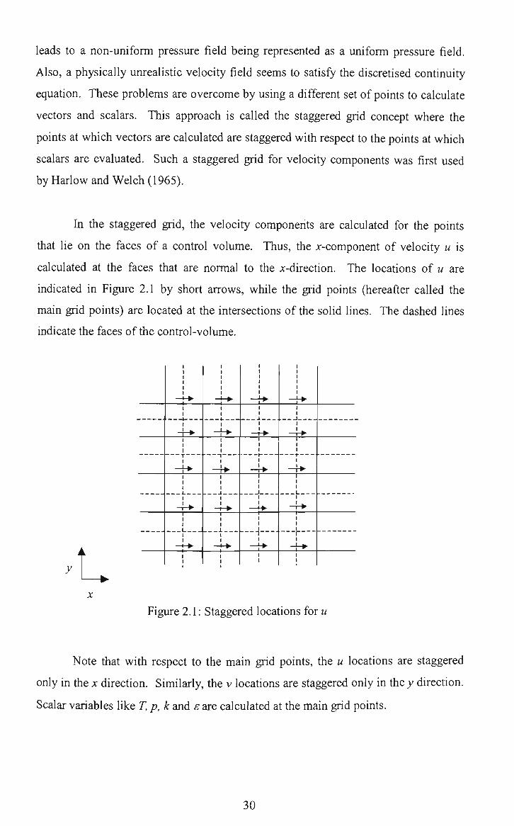
leads to a non-uniform pressure field being represented as a uniform pressure field.
Also, a physically unrealistic velocity field seems to satisfy the discretised continuity
equation. These problems are overcome by using a different set of points to calculate
vectors and scalars. This approach is called the staggered grid concept where the
points at which vectors are calculated are staggered with respect to the points at which
scalars are evaluated. Such a staggered grid for velocity components was first used
by Harlow and Welch (1965).
In the staggered grid, the velocity components are calculated for the points
that lie on the faces of a control volume. Thus, the x-component of velocity u is
calculated at the faces that are normal to the x-direction. The locations of u are
indicated in Figure 2.1 by short arrows, while the grid points (hereafter called the
main grid points) are located at the intersections of the solid lines. The dashed lines
indicate the faces ofthe control-volume.
y
Figure 2.1: Staggered locations for u
Note tiiat with respect to the main grid points, the u locations are staggered
only in the x direction. Similarly, the v locations are staggered only in the> direction.
Scalar variables like T, p, k and e are calculated at the main grid points.
30

The finite volume method can be explained by considering a two-dimensional
convection-diffiision equation for an unknown scalar, (p{=T,k or e):
dtp dt
+ div^ = 5 (2.45)
where, ^ is the flux vector and S is a source term. ^ is the sum of a convection
component t," = putp and a diffusion component " =-p'^V(p. Note that the extia
terms in the momentum equations occurring due to the presence of the porous
medium (the Darcy and Forchheimer terms in Equation (2.21)) are part ofthe source
term. Equation (2.45) is integrated over the finite volume around grid point (/, j). In
Figure 2.2, an example of a control volume for a scalar quantity, is given to illustiate
the discretisation process.
A
Figure 2.2: Shaded area representing a scalar contiol volume.
Rewriting div ^ as fluxes, / , through the sides of the (/, _;>volume with the help of
Gauss' divergence theorem one obtains:
j ^dy^ \[r -f-]iy^ [[f^ -f'^= \Sdxdy (2.46) vol.(;,y') side side vol.(/,y)
The superscripts E, W, N and S refer to the east, west, north and south sides of the
volume respectively. The integrals are approximated as follows:
dtp dt ^^y + [fMn.j - fi-xn.jK + [fi.j^v2 - fi.Hn\^ = S^jAxAy (2.47)
'./
31

Note that the integration is performed over finite volumes around the staggered grid
points for the velocities u and v if the momentum equations are considered.
The integration of Equation (2.47) with respect to time is carried out fully
implicitly (unless otherwise mentioned) by evaluating all spatial derivatives at the
new time level n. The unsteady term, fluxes and source are further discretised using
finite differences. The unsteady term at the time level n is discretised with two time
levels giving a first-order tmncation error in time as follows:
dcp
~dt
n-\
ht • + 0{At) (2.48)
The source term and the diffiision part of the flux are discretised with a second order
tmncation error as follows:
fiu2.j = -\{KJ + pt,f'''''~'^''^0(Ax') (2.49)
The convection flux can be rewritten as:
fUj=(p^);..2y (2-50)
where ^ is an approximation for ^ at the east side of the volume (/, j). Different
approximations for are proposed in the literature. Three examples are given
below:
1. Second-order central scheme
9'-(<P,j+9>.u)^^ (2.51)
2. First-order upwind scheme
(2.52)
3. QUICK scheme (Quadratic Upstieam Interpolation for Convection
Kinematics) intioduced by Leonard (1979a)
K ; +^:>.,y)/2-(^,_,,v - 2 ^ , j +^,>,,y)/8 i f ",.,/2j ^ 0 ^^^
((Pi.j + (PMJ)/ 2 -((p,j -2p.,,j + (p,,,j)/ 8 i f i/,„/,,^. < 0
E (P =
^Ki
i^'>lj
i f « H l / 2 j ^ 0
if ",+1/2 J < 0
9'=\
There are several other schemes such as the Leonard difference scheme, the
power law scheme (Patankar, 1980), the fourth order central scheme and the second
order upwind scheme which have been used to discretise the convection term. The
32

choice of a particular scheme depends on the numerical accuracy required and the
stability offered by the discretisation scheme. For example, schemes 1 and 3 above
lead to a second order tmncation error in the approximation of div ^, whereas scheme
2 gives only a first order accuracy. Strictly speaking, this tmncation error holds tme
only when a uniform grid spacing is used. Solutions obtained by using the cential
scheme exhibit local oscillations if the grid Peclet (or Reynolds) number,
{Pe = pjuJAx I p^) becomes larger than two. These oscillations can be suppressed by
using an upwind scheme such as 2 or 3. The first order upwind scheme most
effectively damps oscillations albeit with an increase in the tmncation error. This
scheme also suffers from a large artificial numerical diffusion.
The hybrid scheme uses a combination of the central and first order upwind
schemes. It is more stable than the central scheme, at the same time being more
accurate than the upwind scheme. If the grid Peclet number exceeds the value of two,
the hybrid scheme locally switches from the second order central scheme to the first
order upwind scheme, and hence, the diffusion contribution is set to zero. The second
order central, first order upwind and the hybrid schemes are used throughout this
thesis.
2.5.2 Grid distribution
In this thesis, grids are generated using algebraic functions. These grids can
either be uniformly or non-uniformly spaced. The staggered grid points are first
developed. They are represented as xu(i) and yvQ) in the x and v directions,
respectively. The main grid points are then calculated by using the staggered grid
locations. Figure 2.3 shows the staggered and main grid locations xu(i) and x(i),
respectively, for the x direction on a 7x7 grid. For discretising the boundary
conditions, tiie grid is extended across the boundaries, intioducing virtual grid points.
In Figure 2.3 tiie heavy solid lines represent the virtual grid, whereas the heavy
dashed line represent the physical boundary. The use of virtual grid points has die
advantage tiiat no modification ofthe discretisation ofthe equations is required in the
volumes along the boundaries.
33

A Dirichlet boundary condition for u velocity on the west or east boundary is
treated by assigning the value to the unknown at the boundary. Similarly, the value
for V is assigned to the unknown at the north and south boundary. Dirichlet boundary
conditions for the scalars are discretised with second order accuracy by using the
virtual point. For example:
(P Dir • + (9(AX') (2.54)
where /max+1 denotes the virtual point.
The discretisation of Neumann boundary conditions with virtual points is
straightforward, and it can be written as:
r /max+l . <PNe,.= — ^ + 0(AX ) (2.55)
I
. _ 1
— r
r
x(I) xu(2) x(2) xu(3) xu(6) x(6) xu(7) x(7)
Figure 2.3: Main and Staggered grid locations for a 7x7 grid
34

2.5.3 Solution ofthe discretised equations
The discretised partial differential equations represent a non-linear system of
algebraic equations. Because of the non-linear nature of the equations, a direct
method of solving the equations entails large computer storage, and it is not preferred.
There are several iterative methods to solve the system of equations such as the
Gauss-Seidel method, the Alternating Direction Implicit (ADl) method introduced by
Peaceman and Rachford (1955) and the Strongly Implicit Procedure (SIP) described
by Stone (1968). For the present study, the line by line Gauss-Seidel method is used
that employs a combination of the Tri-Diagonal-Matrix Algorithm (TDMA) for one-
dimensional situations and the point by point Gauss-Seidel iterative method.
2.5.3.1 The Tri-Diagonal-Matrix A Igorithm (TDMA)
The following is a description ofthe TDMA for the one dimensional case:
The discretised form of the equation that governs the variable cp in one dimension is
written as,
di(Pi =a,(p,^,+b,(p,_^+c, (2.56)
in which a, b, c and d represent coefficients of the discretised equation for variable (p.
Subscript / represents a counter for space, i=imin, imax. The TDMA algorithm
consists of a recurrence formula for the variable in question so that one can obtain the
new value for q) with the help ofthe boundary conditions.
For the forward substitution process, one seeks a relation, ofthe form
V:=P,^,.x^Q; (2-57)
With /=/-/ in the above relationship one can arrive at an equation for cpi-i,
^ M = ^ - , ^ , + a - . (2.58)
35

Substitution of Equation (2.58) into Equation (2.56) leads to,
d^cPi = a,(p,,, + b, {P,_,(p, + a_i) + c,- (2.59)
If Equation (2.59) is rearranged to take the form of Equation (2.57) and the
coefficients are compared, one arrives at a recurrence relationship ofthe form,
^i-biPi-i
For i=imin, the recurrence relations (2.60) and (2.61) give definite values for
Pmin and Qmin. Similarly for i-imax, the recurrence relations give definite values for
Pmax and Qmax- Au explanation for a specific boundary condition with temperature as
the variable is given in Patankar (1980).
Summary ofthe algorithm
1. Calculate Pmin and Qmin using the left boundary conditions (i.e. for i=imin)
2. Use the recurrence relations (2.60) and (2.61) to obtain Pjand ig, for i=imin+I,
imax.
3. Equate the right boundary conditions (i.e. for i'^imax) with Pmax and Qmax-
A. Use Equation (2.57) for i=imax-l, imin to obtain cpimax-i. (Pimin-
For the two dimensional situation, one needs to use the Gauss-Seidel point by
point method along with the TDMA. The general discretized equation in two
dimensions can be written as:
Upcpp = a^(p^ + a^tp^y + a^^cp^ + a^cps + b (2.62)
where ap, aE, aw, a^ and as represent coefficients associated with the variable tp, and b
represents the discretised source term. In order to be able to use the TDMA, one has
to choose a particular direction for one sweep and assume the other direction to be a
constant. For the present simulations, the 5'-A/ direction is chosen for calculations, and
die W-E direction is assumed to be constant for every sweep. Thus, a new source term
36

bo is introduced which contains the terms in the W-E direction. Equation (2.62) is thus
modified to become,
ap(pp = aj^q)^ + ttsCps + bo (2.63)
where b^ = a^cp^ + a^^cp^y + b.
2.5.3.2 The line by line Gauss-Seidel method
The line by line scheme can be visualized with reference to Figure 2.4. The
discretization equations for the grid points along a chosen line are considered first.
These contain the values of tp at the grid points (shown by squares) along two
adjacent lines. If these cp's are substituted from their latest values, the equations for
the grid points (shown by circles) along the chosen line would look like one-
dimensional equations, and they could be solved by the TDMA. This procedure is
carried out for all the lines in the i'-iV direction.
• O -Q-
-0
• o -
• Q
-o- -D
-o-
-O-
-O-
o- -o-
0-
o-
-0-
-o -D-
Figure 2.4: Representation ofthe line by line Gauss-Seidel method.
2.5.3.3 The SIMPLE algorithm
The pressure does not appear explicitiy in the continuity equation, Equation
(2.11). This means that the continuity equation acts as a consfraint on the velocity
field, and the pressure has to be determined such tiiat the velocity field in the
momentiim equation satisfies the continuity equation. The SIMPLE (which stands for
Semi-Implicit Method for Pressure-Linked Equations) class of algorithms uses a
37

pressure-velocity coupling to overcome this problem. A pressure correction equation
is developed which incorporates the continuity equation in the solution procedure of
the Navier-Stokes equation. The main steps in the derivation of the pressure
correction equation are given here (details can be found in Patankar, 1980)
Let j / be the guessed pressure, p the corrected pressure and p the pressure correction
in an iterative solution procedure. Then, one can write:
p = p^+P (2.64)
A similar equation can be written for the corrected velocities, u and v:
u-u^+u , v = v^-i-v' (2.65)
where i / and \^ are the guessed velocities, and u and v are the velocity corrections.
The velocity correction formulae can be written as:
u =djp'^-p'p), V =djp's-p'p) (2.66)
where,
d^=^ andd-'^'^ ap ap
Aew and Ans represent areas associated with the East-West and North-South directions,
respectively. In Patankar (1980), a slightly different formulation is given for the
velocity correction formulae, but both formulations have the same meaning. Equation
(2.66) gives a relationship between the velocity correction and pressure correction.
One can now write Equation (2.65) as follows:
u = u' -hdjp'^-p'p), v = v' +d^{p's-p'p) (2.67)
The continuity equation can be written as:
dp_^d(pul^d(pvl^Q (2.68) dt dx dy
This equation is integrated over the shaded confrol volume in Figure 2.5.
38

-Q-
A • O - -O—
w -o-
o-
Uu
t -Q
-f
r
E O—
Figure 2.5: Control volume for the continuity equation.
For the integration of the term — , the density, pp, is assumed to prevail
dt
over the control volume. Since a fully implicit procedure is used for time, the new
values of velocity and density at time t + At are assumed to prevail over the time step;
the old density, pp at time t, will appear only through the term -—. Thus the
integrated form of Equation (2.68) becomes
(pp-p;)AxAy^^^^^^ - ( /^ l ]^ ;^ + [(pv)„ - ( p v ) > = 0 At
(2.69)
Equation (2.69) is now converted to the pressure correction equation, using
Equation (2.67). The final discretized form ofthe pressure correction equation can be
written as:
Upp'p = a^PE + awPw + (^}^PN + <^sPs + ^ where
«£ = Ptd.Ay,
^s = Psd-s^ >
ap ^a^+a^y +a^ -^a^.
(2.70)
39

= ^ ^ ^ 4 ' ^ + [(p«^).-(p"^).K + [ ( ^ ' l - ( / - ' ) > . (2.70a) M
There are several variations on the basic SIMPLE algorithm such as
SIMPLER, SIMPLEC, SIMPLEST and PISO that enhance the rate of convergence of
the solution for particular flow problems. The SIMPLE algorithm has been found to
be adequate for the present study. A detailed explanation of this algorithm can be
found in Patankar and Spalding (1972). A flow chart explaining the solution
procedure for an unsteady incompressible flow problem using the SIMPLE algorithm
is presented in Figure 2.6.
40

Initialization and Input of Data
I Time Loop for Unsteady Calculations
Guess the Pressure field
I Solve the momentum equations (u and v velocity) to arrive at a guessed velocity
Solve the pressure correction equation
Compute new pressure field by adding the
pressure correction to the guessed pressure
Calculate the new velocities from their old values using the velocity correction formulae
Treat the new pressure
field as the guessed
pressure field.
Solve equations for k, e and T
Figure 2.6: Flow chart of tiie SIMPLE algoritiim.
41

2.5.3.4 Convergence
Since an iterative procedure is used to solve the discretised set of equations, a
relaxation process is required to prevent the solution from diverging, or to speed up
the process of convergence. In the present thesis, this is achieved by using two
methods:
1. Application of a relaxation factor to the variables ( such as u, v, T, k and e)
The solution at the new iteration level is found as:
(p"=a(p'"+(l-a)(p"-' (2.71)
where a is the relaxation factor: a < I leads to under-relaxation, a -1 gives no
relaxation and a > I leads to over-relaxation, (jff" is the solution without any
relaxation.
2. Relaxation with a false time step
The use of an unsteady solution procedure is akin to using under-relaxation.
The term Atp in the unsteady part ofthe tiansport equations, i^(p"j - (p",~j ) / At^, serves
as the under-relaxation.
In order to check whether the solution obtained is a converged solution,
adequate convergence criteria need to be applied (given as the <C.,.. _converged?
symbol in Figure 2.6). For the present study, this is achieved by checking whether the
residual source terms in the discretised equations are below a small stop criterion. As
an example, for the mass sources, the following convergence criterion is applied:
Z Z[(P"),>,/2 J ^e - (P"),-U2.y ^w + {P^lj,V2 ^ " iHj-V2 M ,=2 ; = 2
{NI-2)(NJ-2) < 10"' (2.72)
where NI and NJ represent the number of grids in the x and j directions respectively.
Similar convergence criteria, but including the source terms, are applied to the
momentum and thermal energy equations. In addition to the stop criterion,
convergence was also verified by checking the changes in the variables at specific
monitoring locations between successive iterations
42

2.5.4 Summary
The numerical methods chosen to solve the set of partial differential equations
goveming fluid flow are discussed in this section. Major aspects involved in the
development of the CFD code, including the discretisation of the partial differential
equations, grid distribution and solution of the discretised set of equations, are
explained for a two-dimensional system. In the following chapters, the goveming
equations and the numerical methods developed in this chapter are used with minor
modifications to suit the appropriate physical conditions, geometry and boundary
conditions. These modifications are explicitly stated as they are implemented in the
solution procedure.
Preliminary validation of the CFD code developed for two-dimensional natural
convection flows is presented in the next chapter.
43

Chapter 3
Preliminary validation of the CFD code 3.1 Introduction
To ascertain the robustness and to check the accuracy of a CFD code it is
desirable to validate the code against established benchmark numerical and/or
experimental results. When a code is developed in-house, such as in the present
research, this validation exercise becomes essential. The heating from the side or
double glazing problem of natural convection flow has established benchmarks, both
numerical and experimental. Also, the case study of chapter seven involves natural
convection flow in a rectangular cavity. Therefore, it was decided to employ this
benchmark as a preliminary validation tool for the numerical code written for two-
dimensional systems. The code thus developed can serve as a robust platform to
implement further modifications.
Firsfly, the problem of laminar natural convection flow in a side-heated cavity
is revisited. Air is used as the fluid for all calculations. Comparisons are made with
the benchmark numerical solutions of De Vahl Davis (1983), the revisited benchmark
numerical solutions of Le Quere (1990) and the solutions obtained by Henkes (1990).
De Vahl Davis used a finite difference method of discretisation with a stream
fiinction-vorticity based formulation in his benchmark study. Solutions were obtained
with Rayleigh numbers up to 10 . Due to the lack of computational resources,
benchmark solutions for higher Rayleigh numbers for air, could not be established by
De Vahl Davis. Le Quere used a psuedo-spectral method of discretisation based on
an expansion in Chebyshev polynomials in his benchmark study. This method of
discretisation is known to give more accurate results than the finite difference or finite
volume methods, and thus, the results can be used as a more accurate benchmark. Le
Quere obtained solutions up to a Rayleigh number of 10 and thus extended the
benchmark solutions of De Vahl Davis.
Henkes (1990) used a finite volume method in his investigations as in the
present stiidy. Calculations were carried out for three different discretisation schemes
for the convection flux, namely, second-order central difference scheme, hybrid
44

scheme and first-order upwind scheme. The central difference scheme was found to
give the most accurate solutions. However, the central scheme was also found to be
the stiffest scheme as far as convergence was concemed. The finest grid used was a
120x120 grid with a non-uniform grid distribution. Janssen (1994) extended these
calculations to a 360x360 grid with several discretisation schemes which included a
second-order central difference scheme, fourth-order central difference scheme, first-
order upwind scheme, second-order upwind scheme, QUICK scheme and the Leonard
Difference Scheme (LDS). Janssen (1994) found that for the highest Rayleigh o
number calculated in the steady flow regime, 1x10 , the fourth order cential
difference scheme on a 240x240 grid gave results comparable with the pseudo-
spectral results of Le Quere (1991). The spectral solutions were however obtained on
an 80x80 grid. This result shows the higher accuracy of spectral methods over finite
difference or finite volume methods. However, finite volume and finite difference
methods are easier to implement, and they can be used for complex geometries with o
relative ease. At a Rayleigh number of around 1.7x10 , the flow no longer converges
to a steady flow but oscillates with a definite frequency. This regime has been
described by various authors such as, Paolucci and Chenoweth (1989), Henkes
(1990), Janssen (1994) and Le Quere and Behnia (1998), as the transition regime.
Thus, all calculations for the steady, laminar, natural convection problem are carried
out up to a Rayleigh number of 10* in the present investigation. The finest grid used
in the present study is 120x120, although sufficientiy grid independent solutions were
obtained even on an 80x80 grid.
The present investigation is fiirther extended to the turbulent regime for the
same problem for determining the accuracy of implementation of the k-e model in the
code. In a seminar series organised at the J. M. Burgers Centie for Fluid Mechanics
in 1992 at Delft, Netheriands (Henkes and Hoogendoom, 1992), benchmark
numerical solutions for the turbulent natural convection problem in a side heated
square cavity were sought. The Rayleigh number for the benchmark problem was
fixed at 5x10'°. The experimentally determined turbulent natural convection results
of Cheesewright and his co workers (described in Cheesewright et al, 1986a;
Cheesewright and Ziai, 1986b and King, 1989) at /?a=4.41xl0'° (which is close to
/?a=5xl0'°) in a cavity with an aspect ratio of five, A=5, were used for comparison
witii the benchmark results as this was the most relevant experiment at that point of
45

time. According to Henkes and Hoogendoom (1992), calculations for different aspect
ratios at the same Rayleigh number 5x10* presented in the seminar showed that
differences in the results for A=l and A=5 cavities are very small, provided that the
results are scaled using the enclosure height H as the length scale. For the present
study, the same numerical problem is used, since it is a well established benchmark
problem for turbulent natural convection. The standard k-e model with modifications
for natural convection flows as suggested by Henkes (1990) and Lankhorst (1991) has
been used for the computations.
3.2 Problem definition and governing equations
Figure 3.1 shows the side heated square cavity used for the simulations. In the
Q=0
g
Th Tr H
Q=0
Figure 3.1: Square cavity that has vertical walls maintained at different temperatures and the top and bottom walls are adiabatic.
figure, Q is the heat flux, and it is zero for the adiabatic horizontal walls. Th
represents the temperature of the hot wall. Tc represents tiie temperature of the cold
wall, and H is the length and height of the square cavity. Vector g represents
acceleration due to gravity. Since the heat flux Q involves the first derivative of
temperatiire with respect to space, die adiabatic condition can be mathematically
represented as — = 0 at>^0 and H. dy
46

3.2.1 Non-dimensional equations
gPATH'' Pr For the present problem, the Rayleigh number is defined as Ra =
v"
where AT =T^-T^ is the temperature difference between the hot and cold walls and
C p Pr = —— is the fluid Prandti number (Pr=0.71 for air). In the case of natural
kf
convection flows, for low Prandti number fluids such as gases as well as low viscosity
liquids, the convective acceleration term is balanced by the buoyancy term in the
momentum equation. The goveming equations for buoyancy driven flow in a two-
dimensional system presented in Section 2.4.1.1 of chapter two are non-
dimensionalised in the following manner.
Let the subscript ref represent a reference value for all variables and
superscript nd represent the non-dimensional variable. As a result, one can write:
nd ^ nd ^ qpnd U — , V — , 1
^ref ^ref
nd _ ^ 1 nd _ "• nd _ b — , K — , p —
^ref '^ref
_ ^ 'Pr4 nd _ X — - A •
^ , P"' = ^ , P:' Pref Pref
H
P- fnd _ t
Pref Kef
P
Pref
Using the above non-dimensional variables, one can equate the convective
acceleration and buoyancy terms in Equation (2.31) and arrive at: u^^j- =^gflATH .
By equating the convective acceleration term with the pressure term, one then
obtains:/( ^^ =pw^g . The reference temperature is taken as To=(Tc+Th)/2. The
reference density and viscosity are taken as the fluid density and viscosity,
respectively. The reference time tref, is taken as the ratio ofthe reference length scale IS
and the reference velocity scale, i.e. t,.^^ = . . "^ ^gfiATH
The reference values for turbulence kinetic energy and the rate of energy
dissipation are derived with tiie aid of perturbation theory as described in Wilcox
(1993). kref and eref are given as:
k -U^ p - ^
Al

Using the non-dimensional parameters and dropping the superscript nd from all the
variables, the equations given in Section 2.4.1.1 can be rewritten as:
1. Equation of continuity:
d{pu) ^ d{pv) ^ Q
dx dy (3.1)
Momentum equation in the x direction:
du du du dp ?r d p— + pu — + p v — = —— + A
dt dx dy dx \ Ra dx
[P + PA^ du \]
dx
-i-. Pr d
Ra dy
I ^ du dv
y j
(3.2)
Momentum equation in the>^ direction:
dv dv dv dp IVx d p—+pw — + p v — = —— + A
dt dx dy dy \Rady
dv (/ + /^J2 -y j
+ . Pr d
Ra dx
( M du dv^
y j
AT-T,)
(3.3)
Thermal energy equation:
dT dT dT I d p—+ pu — + pv— = —===—
dt dx dy •sl?rRa dx
P + Pt Vx\dT
J
+ 1
^VvRa dy P +
p,?v
dx
^dT
LV y dy
(3.4)
Turbulence kinetic energy equation:
dk dk dk
dt dx dy
Pr d
Ra dx
+ . Pr d
Ra dy
V
7
L-V
or
dk
J \
cr.
dx
dk
y dy
+ Pk+G,-pe
(3.5)
48

Equation for the rate of energy dissipation:
de de de Pr 5 p— + pu — +/0V— = A "^ dt dx dy \Radx
^ Pt \de dx
LV ^ W
-I-. Pr d
Ra dy
7
LV a
de
J dy
(3.6)
+ {c.J^Pk + c,fii)-pc^J^e)-
with
Pk-Pt
Gk —
\Pr_
Ra
I
f
V
(7^.\^ (PkA^ du + 2
dv_
v ^ y
-1-du dv^ — + — dy dx
Pt dT
-JPrRa (TT dy
Pt = Ra ^ k 2
e
For laminar solutions, Equations (3.5) and (3.6) are not used in the
calculations, and the eddy viscosity, pt, is taken as zero. Variables, u,v,p and T are
instantaneous quantities for laminar calculations. One can use either a steady or
tiansient approach for laminar calculations. In the former case, the time derivatives in
the equations are set to zero.
For turbulent solutions, Equations (3.5) and (3.6) are solved simultaneously
with Equations (3.1) to (3.4). Variables, u, v,p and Tare time-averaged quantities of
calculations that involve turbulence. Here again, one can either use a steady approach
or approach the steady state solution by integrating through time. The time
derivatives in the time averaged Navier-Stokes equation represent the large time
behaviour according to Henkes (1990). The nature ofthe transient solution depends
on the type of turbulence model used. Thus, the tiansient solution may not approach a
tme tiansient for turbulent flow calculations.
In the present simulations, a steady approach is adopted for laminar and turbulent
calculations.
49

3.2.2 Boundary conditions
For calculations that involve laminar flow, natural boundary conditions are
applied for w, v and T. The boundary conditions can be summarised as follows:
u = v = 0 at x = 0and.^
M = v = 0 at j = OandH
T^T^ at x = 0 (3.7)
T=T^ at x = H
— = 0 at y = OandH dy
For calculations involving turbulent flow, using the standard k-e model, wall
functions presented in Section 2.4.1.1.1 of chapter two are not used. As mentioned in
Section 2.4.1.2 of chapter two, standard wall functions, (Equations (2.38) and (2.39)),
developed from simple forced convection flow experiments cannot be used for natural
convection flows. In order to alleviate this problem Henkes (1990) and Lankhorst
(1991) suggested the modification of the standard k-e model near walls. These
authors solved for the mean quantities (w, v and T) right up to the wall, which is
similar to the tieatment adopted in the case of low-Reynolds number k-e models.
However, for the turbulent quantities, k and e, wall functions such as in Equations
(2.43) and (2.44) were used. These wall functions are applied at the first inner grid
point. Since the region close to the wall is extiemely important in calculating heat
transfer rates within the boundary layers, the first grid point has to be located
extremely close to the wall. When this is done, it is reasonable to assume that the
values of k and e at tiie first inner grid point might be obeying the law of the viscous
sublayer (v^ =x' for x"" < 11.63). Therefore, in addition to the wall functions in
Equations (2.43) and (2.44) for ^ and £• obtained from the inertial law (x^ > 11.63),
Lankhorst (1991) developed wall functions for these turbulent quantities within tiie
viscous sublayer. By differentiating the linear velocity profile for the inertial sublayer
and using it together with the defining equation for pi, one obtains altemative wall
functions for k and e as follows (for x^ < 11.63):
(KX\'f k=^ ^^ (3.8)
50

e^- '-^—^ (3.9)
For the present calculations, these two forms of the wall fimctions are used
and compared with the results obtained by Lankhorst (1991) and the experiments of
Cheesewright and his co workers. The mean variables {u, v and T) are solved right up
to the wall. Note that all boundary conditions are used in their respective non-
dimensional forms.
3.3 Numerical methods
The goveming equations are solved using the finite-volume method on a
staggered grid as described in Section 2.5.1 of chapter two. The convection-diffusion
terms are discretised using a second order central difference scheme and a hybrid
scheme for comparison. Pressure and velocity are coupled using the SIMPLE
algorithm, and the line by line Gauss Seidel method is used for solving the discretised
equations. Details of the numerical methods can be found in Section 2.5 of chapter
two. The under-relaxation factors for the variables u, v, T and p were assigned
different values depending on the Rayleigh numbers calculated. As the Rayleigh
number was increased, lower under-relaxation factors had to be assigned to avoid
divergence ofthe solution. The specific values are provided in Section 3.4.
3.3.1 Grid distribution
Non-uniform grid spacing is used for all calculations with fine grids close to
die wall and progressively coarse grids towards the centre of the cavity. At low
Rayleigh numbers, non-uniform grid spacing is not essential. At higher Rayleigh
numbers, one encounters steep velocity and temperature gradients. Fine grid spacing
is required close to the wall to resolve these gradients. The use of non-uniform grid
spacing allows an economical distribution of grids in the calculation domain. For
laminar calculations, a sine function distribution for the x and y directions is used:
^ ( 0 i ^ • (r, i \ . . /-, i m —— = sin 2;r i = imin,imax (3.1U)
H imax 2;r l /max;
51

yv{J) J I H ymax 2;r •sm 2;r-
zmax. y = y mm, j max (3.11)
At the highest Rayleigh number (IxlO ) in the laminar regime and for all calculations
in the turbulent regime, a hyperbolic tangent function is employed for grid
distribution in the x direction. This function enables a finer refinement close to the
wall.
'' tanh{a,[///max-l/2]}^ xu ' 2
1 + -V
/ = / mm, I max tanh(a,/2)
where «/ represents a grid refinement parameter given by:
(3.12)
a, «2 = (3.13)
sinh(«,)
With a low value of a2, one can obtain a fine grid close to the wall. A range of values
of this parameter, 1.0x10" < 0:2 1-0x10~\ is used to study the effect of grid
refinement close to the wall. A representative non-uniform mesh using the sine
functions (3.10) and (3.11) for grid distribution in the x and y directions is shown in
Figure 3.2. In general, the results obtained with an 80x80 grid were found to be
sufficientiy grid independent for both laminar and turbulent cases. However,
calculations are done up to a grid size of 120x120 for the sake of comparison with the
result obtained by Henkes (1990) on the same grid.
1
0.9
0.8
0.7
0.6
go.5
0.4
0.3
0.2
0.1
0
4 1 T " " " ' ^ " ~ ~ ~ ~ •
l | l | | iJ l 4 3||
if 1 1 "i
1 f I ^ m\\\\\\
'" • " " • " "
t
i 1 jl 1 m\\\\
B 1
11 jiljl|||||- = ; ; i = = = i= = = = = E = =
ya^MygW;Litt«i#|
" ' " ! i i-i-..
'WTY-1 : 1 !
i 1 i 1 '.
• 1 1
1, !
; 1
i ;
iif--"^" " - 1 - -r4-i---- • • • [ 1
1 _j+
i
1 1—1 -j |-rl-|-
-Ffi nulliiil
1' '11 jii iilJ -^IliliHl
l i i l i ' 1 i;it 1 1 j 1 11 j IH 1
1 - { 1 i 1
lu 11 1 ) | l || 1 1 ||l 1 i l l
11! H"l ns I I I
1 j H 1' I I 1 1
0 0.5 X/H
Figure 3.2: Representative non-uniform mesh using a sine fimction for grid distribution in the x and y directions.
52
3.4 Results and discussion
In order to verify the accuracy of the solutions some important parameters are
monitored for each calculation. These are:
1. Non-dimensionalised heat transfer from the hot wall which is referred as the
Nusselt number.
(dT\ Nu = - -
ATydx (3.14)
y hotwall
Stratification at the centre ofthe cavity
H S =
AT
fdT^
3. Non-dimensionalised maximum ofthe vertical velocity at the horizontal mid-
plane of the cavity.
""- (3.16) ^gJ3ATH
A. Non-dimensionalised maximum of the horizontal velocity at the vertical mid-
plane ofthe cavity.
""^ (laminar flow), - ^ = ^ ^ = (tiirbulent flow) (3.17) (g/3ATvf ^g^ATH
3.4.1 Laminar flow solutions
3.4.1.1 Stieamlines and isotherms
In Figure 3.3, simulations are presented for increasing Rayleigh {Ra) numbers for air
in tile laminar regime, starting from i?a=10^ up to 10^ Frames (a), (c), (e), (g), (i) and
(k) in tiie figure represent isotherms, whereas frames (b), (d), (f), (h), (j) and (1)
represent the corresponding sfreamlines for Ra=lO , 10, 10, 10, 10 and 10 ,
respectively. As the Rayleigh number is increased from very low values (almost
stagnant fluid for Ra < 10 ), natiiral convection flow in the square cavity begins. At
y?a=lO^ and lO"* (Figures 3.3(a) to (d)), one can see a bending ofthe isotherms from a
vertical position indicating the effect of natural convection on the temperature
53

pattems in the cavity. A single clockwise rotating cell is formed at these Rayleigh
numbers as seen from the streamlines (Note that the left wall is hot and the right wall
is cold, and therefore, the motion is in the clockwise direction). The under-relaxation
factors used for this set of simulations were: Uurf = 0.5, Vurf - 0.5, T^rf =0.5 and purf -
0.8.
As the Rayleigh number is increased to Ra=lO^ and 10 (Figures 3.3(e) to (h)),
the bending ofthe isotherms is enhanced further. At Ra^lO^, the originally vertical
isotherms are almost horizontal in the central portion of the cavity as seen in Figure
3.3(g), indicating strong natural convection currents. The isotherms are closely
spaced near the vertical walls indicating steep gradients close to these walls. The
stieamlines for Ra=lO^, Figure 3.3(f), show the splitting ofthe single clockwise cell to
a two cell pattem with a saddle (or no flow) point at the centre of the cavity. At
Ra-lO^, the streamline pattem again changes, now showing three clockwise rotating
cells with two saddle points, as seen in Figure 3.3(h). The closeness of the
stieamlines near the vertical walls again indicates steep velocity gradients near these
walls. The under-relaxation factors used for this set of simulations were: Uurf= 0.3,
Vurf= 0.3, Turf= 0.3 andpurf= 0.5.
With a further increase in Rayleigh number to /?a=10 and 10 (Figures 3.3(i)
to (1)), the stieamlines and isotherms become very closely spaced near the vertical
walls. The centre of the cavity is, however, quite stagnant with an almost no flow
region. At these high Rayleigh numbers, the streamlines have split into several
clockwise rotating cells as seen from Figures 3.3(j) and (1). The central portion ofthe
cavity still has three clockwise cells and two saddle points. However, the upper left
and lower right comers of the cavity have developed strong rotating cells or vortices.
Similar flow pattems were observed by Henkes (1990) in his calculations with air as
die fluid. At these Rayleigh numbers, significantly low under-relaxation factors had
to be used to allow the solutions to reach a final converged steady state result. These
were: Uref= 0.1, Vref= 0.1, Tref= 0.05, pref= 0.1. This was particularly the case with the
cential difference scheme of discretising the convection-diffusion terms.
54

(a) (b)
(c) (d)
Figure 3.3 (For caption, see page 57)
55

(e) (f)
(g) (h)
Figure 3.3 contd. (For caption, see next page)
56

(i) G)
(k) (1)
Figure 3.3: Numerical prediction ofthe flow field for increasing Rayleigh numbers for air in the laminar regime. Frames (a), (c), (e), (g), (i) and (k) represent isotherms whereas frames (b), (d), (f), (h), (j) and (1) represent streamlines foTRa=lO\ 10\ 10^ 10^ 10 and 10Vespectively.
57

3.4.1.2 Accuracy ofthe solutions
Table 3,1 indicates the accuracy ofthe solution for air at Ra=lO^, 10'* and 10 .
Non-uniform grids were used for all these Rayleigh numbers, although it is not
essential to do so at lower Rayleigh numbers. Parameters given in Equations (3.14) to
(3.17) were monitored for all Rayleigh numbers. For the simulations, 30x30, 40x40,
60x60 and 80x80 grids were employed for each Rayleigh number. The convection-
diffusion terms were discretised by using the second order central scheme. Results
have been compared with the benchmark numerical solutions of De Vahl Davis
(1983), (referred to as DVD in the tables). As seen from the Table, the present
solutions compare well with the results of De Vahl Davis. If one compares the
present results at the largest grid size to the benchmark, the maximum deviation in Nu
is 0.17% (for Ra = 10 *), in Umax is 0.20% (for Ra = lO" ) and in Vmax is 0.52% (for Ra =
10'*). De Vahl Davis does not provide values for the stratification, and therefore, a
comparison could not be made. One can also see from Table 3.1 that as the grid size
is increased, the solutions tend to a grid independent result.
Table 3.2 presents the accuracy ofthe solution for air at Ra-lO . The central
difference scheme is again used for all simulations. Calculations are performed up to
120x120 grids. The results obtained are compared with the benchmarks of De Vahl
Davis (1983), Le Quere (1990), (referred to as LQ in the tables) and the results of
Henkes (1990) at the highest, 120x120, grid calculated by the author. From the
tables, it can be seen that the present results are in general close to the results obtained
in all previous studies. In particular, the present solution with the 120x120 grid is
closer to the benchmark of Le Quere who used a more accurate pseudo-spectral
method. The present results are also in close agreement with the results obtained by
Menkes (1990) who used a finite volume method as in the present thesis. With the
finest grid, the present results have the following deviations from the results of Le
Quere and Henkes:
in Nuavg, 0.07% (LQ), 0.11% (Henkes),
in Umax, 0.32% (LQ), 0.34% (Henkes),
in Vmax, 0.11% (LQ), 0.00% (Henkes),
in Sc, not available (LQ), 0.04% (Henkes).
58

o
a c
"o
u
o o 2 3 o u <
o / " N
^ 1 ^ CO I ' ^
\ _^ ^
1^
II
Co"
V m
ax
t<
e a
£ ;^ ^ tX)
;^
| 0
1 • ^
' ^ ' ^ N
§p a
1
T3
"C o
(U
c
Sch(
1
ayle
igh
umbe
r
&i z
O N
,528
o
00 en 1—1
o
r-00 i n • ^ .
o
00 oo OS J—^
o
00 r — <
. — (
o m X o m
BJ )-( -t-i c (U U
o 1—(
X
00
529
o
o ON m «—H
o
o o so "^ o
00 00 ON ^^ o
00 . — 1
.—'
o ^ X o ^
(S l-l
4 - »
c u u
m O * — « X
VO
526
o
o ON m ^^ o
o oo i n ' ^ o
oo oo OS — 1
o
oo ^^ — 1
o MD X
o VO
CO VH
4-»
c u u
o 1—(
X
00 ,5
22
o
oo oo m . — ( o
f O ON i n ' ^ o
oo oo ON 1—(
o
oo . — ( - — 1
o oo X o oo
a t-c *-> a (U O
O 1^-^
X
t ^
847
o
00 ' ^ en f N O
OO ON <N ON O
r-xf Csl CN
o
r-^ <N CN
o m X
o en
cS u G C <u U
o 1—4
X
OO I—1
oo d
m r r m CNl
d
ON
en ON
d
V£) r f CN CN
d
vo •^ CN CN
O Tj-X o ^
Kl i3 a (U
U
o 1—(
X
r-
837
o
i n CM en ( N
d
^ ( N ^ ON
d
CN '=*• CM CM
d
rsi ^ CN CN
o VO X o ^
CO i-i +-» c (U
U
1 -
o 1 - ^
X
' ^
834
o
i n en en CN
d
vo en ^ OS
d
ON en CM CM
d
CJN en CN CM
o oo X
o oo
CO i-l
4->
d <u O
o 1—H
X
i n i n p ' '
r-i n CM
d
en vo en ON
d
i n ^ i n rsi
d
vo Csl m 'si-'
o en X
O en
CO u -4-»
c <L> U
i n O f—H
X
.061
. — <
CN (^ i n CN
d
r-t~-en ON
d
T f ^ m ( N
d
^ CN i n
^"
o ^ X o ^
CO u -t-"
c (L)
u
O 1 - ^
X
i n O
*""*
o t-^ i n rs j
d
r-oo en OS
d
CN • ^
i n CN
d
o CN i n
^ '
o so X
o so
Fl i2 c <u u
o .—( X
*n so p ^
o oo i n CN
d
oo o ^ ON
d
o ^ f i n rs)
d
so 1 — *
i n
' ^
o oo X
o oo
CO u - t - ;
a <U
u
O r—r
X
l > 00 en < — ( d
i n oo i n ^ d
oo oo OS • — '
d
oo . - H
" — I
o D
^ ^
en CN en CN
d
i >
.— 'sl-Os
d
en ^ CN CN
d
en ^ CN CN
f o Q
^§
^ r-i n CN
d
o o ^ Os
d
•? >n rs j
d
Os
^^ <n '^'
1
" o Q ^ > - B

so
o <3
Q<
CO u
'co
C
_o
"o 00
o
•5 O O CO o o < CN
rn 0)
1
tJ
^^ "N
CO 1 fo^ V >
tI3 E-x <]
II
CO
^ p
>
>£ §
3
£ ^ ^ bo
m
^ E- < ^ bo
to 13
1 • ^
— S3
<; "*.<
bo a
1
T3
'C 0
U
Sche
m
W) u
ayle
i um
b
Qi ==
CJS en ^O ON
d
r-so i n CM
d
0 0 ON r-d
CN r-r~ CM
d
so so C-~;
00
0 CN X
0 (N
CO
C 0)
0
0
0 T — <
X
I ^ ON en ON
d
so ^ i n CM
d
i n so ON r-d
0 00 t ^ CM
d
r4 ON !>; ocj
0 en X
0 en
CO ^ C (U
a
vO
0 T—H
X
-< 00 <N o\ d
i n ON i n ra d
t--so 0 00
d
i n 00 t~-CN
d
00 0 00 00
0 '^ X 0 ^
CO h c ii
u
• 0
0 1—I
X
en C3N »—I
ON
d
C--CM SO r^i d
ON CN 1—(
00
d
00 00 r~ CN
d
r-r—*
00 0<j
0 so X
0 SO
CO
a & <U U
vO
0 T—1
X
' t so .—I
OS
d
00 1 - ^
so CM
d
0 en y-^
00
d
0 ON r-Csl
d
<N CN 00 00
0 00 X
0 00
CO i i c (U U
so 0 1 — <
X
0 • ^
1—i
0\
d
CM SO CM
d
CM r-»-H
00
d
en ON r~-CM
d
i n en 00 00
0 CN f—H
X 0 Csl
CO
u d (U U
so 0 f - H
X
en 0 so CN
d
rs) » - H
00
d
en 00 r-~ rsi d
0 0 00 00
°9 ^^
00 ^ - H
SO rsi
d
VO
^ r—1
00
d
0\ t>-CM
d
so rsi 00 00
x>
2 a X J
'^ • ^
^ C:N
d
CM SO CM
d
^ ^ y—t
00
d
0 Os r-CM
d
rsi rsi 00 0C3
0 rsi » - H
X 0 rsi
"rt 4 - *
c (U U
•" 0 (11
1x10
(H
enk(

Thus, the maximum deviation in the results is less than 0.5%) for all parameters. The
stratification value was not provided by either Le Quere or De Vahl Davis. Therefore,
the present results for stratification were compared with those of Henkes, only.
Table 3.3 presents the results obtained for Ra=lO . The central and hybrid
differencing schemes were used to discretise the convection-diffusion terms in this
case. Since De Vahl Davis (1983) has not provided any results for this case,
comparisons have been made only with the results of Le Quere (1990) and Henkes
(1990). From the table, it is clear that the cential scheme is superior to the hybrid
scheme in terms of accuracy. However the central scheme was found to be extremely
stiff at such high Rayleigh numbers, and significantly low under-relaxation factors
had to be employed to arrive at a steady converged solution. Following are the
deviations calculated with the central and hybrid schemes for the finest grid in
comparison with the benchmark of Le Quere and the finite volume solutions of
Henkes.
Cential scheme: Hybrid Scheme:
in Nuavg, 0.30% (LQ), 0.20% (Henkes), Nua^g, 0.53% (LQ), 0.10% (Henkes)
in Umax, 0.95% (LQ), 4.86% (Henkes), Umax, 7.57% (LQ), 1.47% (Henkes)
in Vmax, 0.30% (LQ), 0.04% (Henkes), Vmax, 0.4171 (LQ), 0.04% (Henkes)
in Sc not available (LQ), 0.05% (Henkes), Sc not available (LQ), 0.05% (Henkes).
The maximum error between the benchmark and present solution occurs for the
maximum ofthe u velocity, and it is as much as 7.57% for the hybrid scheme. For the
central scheme, all errors are below 1% compared to the benchmark of Le Quere
(1990). Although the present results for the maximum of the u velocity deviate
significantly from the benchmark for the hybrid scheme, these results are more
accurate tiian tiiose of Henkes (1990). To put it in context, the results of Henkes
deviate by as much as 5.54%) for the cential scheme and 8.92%) for the hybrid scheme
(for die maximum of the u velocity) from the benchmark. Further calculations were
not carried out in the laminar regime, since a converged solution could not be
obtained beyond a Ra=lO^ with tiie cential scheme. Previous studies have also found
that a Rayeligh number of approximately Ra=lO^ represents the limit of the laminar
flow regime for air in a side heated square cavity.
61

00
o
T a CO
"a
C O
O m (U
-4-t
o
CJ CO
3 O o < en en
i
o r E-i
^
^
1
•o
^ 9
>
^ §
s
60
a
1
6fl
1
TS "C o
6 J3 o
-§ C
" ^ CO
0^
N
c ^
<I 1
£ 1^ ^ bo
ro
> E-.^ < ^
v j ^
TT
.-C3
i
CM en en C3N
d
CM rsi rsi
d
en »n o i >
d
o so oo rsi d
o so ocj rsi
o CM X
O CM
%
U
>0
O
"x
CM
ON ON
d
-^ ON so Cs4
d
CN SO CM t~-
d
ON ON ON r-1 d
ON ON
ON rsi
o T f X o ^
CO
i3 % U
oo o X
rl-<?s ON
d
• ^
so rsi
d
o oo ' ^ r-d
en t—.(
o en d
en ^^ d en
O so X
O SO
U
oo o "x
rs|
O N ON
d
T—)
<n so r^ d
Tj-ON r-d
i n ^—( o rn d
i n . — 1
d en
o 00 X o oo
CO H
% U
oo o X
. — 1
oo en O N ON
d
i n •^ so rsi
d
1—1
en so oo d
xt-
o en d
"^
d en
O CM V - H
X o r4 ^^
CO H
o
0 0
O
X
en <?s C3N
d
so ' ^ SO rsj
d
en CN 00
d
o CN o en d
o CM
d m
O CM 1—4
X o rsi 1—1
CO H ^ U
U
X § ^ E.
en o en oo d
en • *
n rsi
d
so r~-so 00
d
en • *
t~~ o l d
en '^f r- O l
o CM X o CM
no
- ^ K
» o 1-H X
rsj vn C3N
d
rsi o c^ rM d
oo CM i n r-d
<7s i n ON rsi
d
O N i n C3N rsi
o ^ X
o • ^
-TO
f. K
oo o ' x
CM
r~-C3N
d
ON CM SO Csl
d
en r-r-r-d
oo oo Os CM
d
00 0C3 ON r^
o so X O SO
f. E
oo
o r—< X
r--i n
ON
d
oo i n so rsi
d
oo 00 Os r~-d
ON ON rsi
d
Os ON
r i
o oo X
o oo
-R K
oo o !<
en o 00 ON
d
oo - * so CN
d
^ i n o oo d
r-o o en d
r-o d en
O r^ . — t
X o CM
f. E
oo o "x
oo o oo ON
d
ON
•^ so rsi
d
r-en ON r--d
o ^^ o en d
o • — 1
d en
o rsi » — * X o rsi
•c ^ E
» 4)
2-^ X a3 ^ K
t~-en so CM
d
T ^ . - H
r-oo d
en rs| o en d
en CM
d en
•JO ^ _ ^
2 a

3.4.1.3 Effect of grid distribution on accuracy
In order to present the effect of grid distribution on the accuracy of the
solution, fiirther calculations were carried out at Ra=lO^ by using the hyperbolic
tangent function in Equation (3.12) as the grid distribution function in the x direction.
For the y direction, the sine function (Equation (3.11)) was maintained. The hybrid
scheme was used to discretise the convection-diffiision terms. As mentioned earlier,
with a low value of a^ in Equation (3.13), one can obtain a fine grid close to the
vertical walls. Therefore, the value of a2 was varied between I.Ox 10"' and 1.0x10'
for the present study. The grid size is maintained at 80x80 for all calculations.
Comparisons are made with the benchmark results of Le Quere (1990) for all
parameters except the stratification. For stratification, the results obtained in the
present study with the 120x120 grid and the central scheme are used as a benchmark.
The results are summarised in Table 3.4. For 0 2= 1.0x10"', the results obtained are
closest to the benchmark for Nuavg, Umax and Sc, but not for Vmax- As the value of a^ is
decreased, the results show an improvement for Vmax with a slight deterioration in the
predictions for the other parameters up to a2=1.0xl0""'. With a further decrease in the
value of a2, however, the predictions begin to deteriorate significantly as seen from
the results for «2=1.0xl0"^ and 1.0x10" . These results clearly show that the accuracy
ofthe solution depends greatly on the grid distribution in addition to the total number
of grid points.
3.4.1.4 Variation of wall heat transfer and stratification
Henkes (1990) calculated the variation of wall heat fransfer and sfratification
for air using the boundary layer equations as well as the full Navier-Stokes and
thermal energy equations. Henkes (1990) found that for the laminar regime the
sfratification asymptotes to a value of 0.99 (at Ra = 10 ) with the boundary layer and
Navier-Stokes solutions. The average wall heat transfer asymptotes to the relation:
iVw , =c/?a'"'where c = 0.30 and 0.31 with the Navier-Stokes and boundary layer
equations, respectively. As seen from Table 3.3, the results for Ra= 10 indicate the
same asymptotic behaviour for the present simulations. This asymptotic behaviour
63

for sfratification and average wall heat transfer with Rayleigh number in the laminar
regime for air is also seen in Figures 3.4(a) and (b), respectively.
Table 3.4: Effect of grid distribution on accuracy (an 80x80 grid is used for all calculations).
Scheme
Hybrid
Hybrid
Hybrid
Hybrid
Hybrid
Hybrid
Hybrid
Ref
(LQ)
/y — !
sinh(a,)
1.0x10"'
l.OxlO"^
2.0x10"^
1.5x10"
1.0x10"
1.0x10"^
1.0x10"
NUavg
30.07
29.96
29.90
29.90
29.87
30.55
48.05
30.23
Ra'"
0.3007
0.2996
0.2990
0.2990
0.2987
0.3055
0.4805
0.3023
" n ^
{gfi^TvT'
0.7958
0.7918
0.7902
0.7892
0.7888
0.7868
0.7852
0.8714
V max
•sIgflATH
0.2651
0.2650
0.2645
0.2647
0.2655
0.2640
0.2671
0.2637
AT[dy) c
0.9786
0.9749
0.9735
0.9744
0.9733
0.9732
0.9667
0.9938 (present)
In Figure 3.5, the variation in the local wall heat transfer, for the hot wall, is
presented for different Rayleigh numbers for air. In this figure, y/H = 0 and 1,
respectively represent the bottom and top of the square cavity. It is seen from this
figure that with an increase in the Rayleigh number, the heat tiansfer from the bottom
half of the hot wall progressively increases. This increase consequentiy leads to an
enhancement in the average wall heat fransfer with Rayleigh number.
64

CO
Ra
(a)
Ra (b)
Figure 3.4: Variation in the (a) core stiatification (b) average wall heat transfer with Rayleigh number for air in the laminar regime.
65
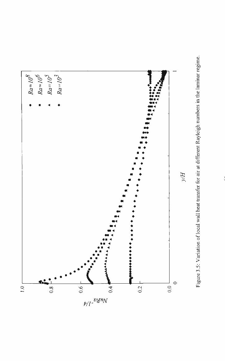
lU
oo o II
Q-
«
D
so i n <^ O 05 o "^ "^ •"*.< II II II a a a
0:^ C< 0:^
• .4 •
• . « . ^
% 1 i J§
4sa.4
4M'4 « . 4 •1.4
mt • •
• < • • < •
« •
« •
• •
• •
• •
• •
« •
• •
• •
« •
•1 •
• •
•4 • • 4 •
«M • •1.4 •
• .4 • « i .4 •
M .4 • • • .4 •
• • .4 • • • .4 •
• • .4 • • • .4 •
• • .4 • • • .4 •
• • .4 • • • .4 •
* • i T p • i -i t
, • ' * . • •>
'• ^ p ' 0 0
d
*. •!. ^ \ \ 1 ' H — ' ^ V
so '5j- CN <5 d d
f
t—s
p c D
y/H
bO
arre
c
lam
i in
the
Var
iatio
n of
loca
l w
all h
eat t
rans
fer
for
air
at d
iffe
rent
Ray
leig
h nu
mbe
rs
i n en <D hi S) '£
p/f v^nfq

3.4.2 Turbulent flow solutions
Turbulent natural convection flow is still an active research area from both
experimental and computational points of view. Experimentally, it is difficult to
constmct a setup which can be used to study high Rayleigh number natural
convection especially with air at atmospheric pressure. Such an experimental setup
needs to be at least as large as the size of a standard room. In order to overcome this
problem, some authors have studied natural convection either at high pressures or by
using a high Prandti number fluid. Even when such experiments are conducted, the
application of boundary conditions, such as the adiabatic boundary condition, is not a
trivial task. Therefore, it is difficult to compare the experimental results with a
numerical simulation that uses ideal boundary conditions. In order to overcome such
difficulties, a standard test case was suggested by Henkes and Hoogendoom (1992),
to test the accuracy of turbulence models for natural convection flows. The standard
test case involves the study of a side heated square cavity with air at /?a=5xlO'° by
using the standard k-e model. Several authors provided their numerical results for
this test case, and the results were compared with the experimental results of
Cheesewright and his co workers. For the present calculations, this test case is used
as a validation exercise for the implementation of the turbulent flow model. It should
be emphasised here that since the implementation of a turbulence model and the
associated boundary conditions can vary significantly from one study to another, the
validation exercise with turbulent flow calculations is not as rigorous as that with
laminar flow calculations. Nevertheless, the validation still provides sufficient
confidence while using the code for fiiture turbulent flow calculations.
Turbulent natural convection flow problems, such as the present one, have
been known to have numerical problems with convergence. In the present case,
initially, an unsteady procedure was adopted to arrive at the converged solution. The
unsteady solution was found to be more stable due to the use of false time stepping
which acts as an under relaxation. However, a significant amount of time was taken
to arrive at a final converged steady solution. In order overcome this problem, a
steady solution procedure was adopted starting with relatively high under-relaxation
67

factors to induce turbulent flow with Uurf = 0.5, Vurf = 0.5, Turf = 0.5 and purf = 0.5.
The number of Gauss-Seidel sweeps between each iteration was also increased to 10
sweeps for the velocities and temperature (from one for laminar calculations) and 30
sweeps for the pressure (from three for laminar calculations). For the turbulent
quantities, k and e, again 10 Gauss-Seidel sweeps were employed. The required
number of Gauss-Seidel sweeps were ascertained after a trial and error procedure, and
the above number of sweeps were found to be the lowest to obtain a converged
solution. After approximately 500 iterations, when the solution stopped converging,
but started giving oscillatory behaviour, the under relaxation factors were decreased
significantiy to «„,/= 0.1, v„^= 0.1, Turf= 0.1 and purf= 0.2. The Gauss-Seidel sweeps
were kept constant for the entire period. This procedure ensured a converged steady
solution.
1 n
For the test case of Ra=5xlO , square cavity, the boundary conditions for the
mean and turbulent quantities were modified for natural convection. Henkes and
Hoogendoom (1992) suggested that the mean and turbulent quantities be solved right
up to the wall without the use of any wall functions. For the mean quantities, the
boundary conditions given in Equation (3.7) were used. Instead of using wall
functions for k and e such as in Equations (2.43), (2.44), (3.8) and (3.9), these authors
used k= 0 and e~^co at the wall for the test case (here, oo implies the use of a large
value of e at the wall). In the present computations, however, the use of f- oo at the
wall did not lead to a converged solution. Therefore, it was decided to use two sets of
wall functions for A: and ^ provided by Equations (2.43) and (2.44) (hereafter referred
as SBCl) and (3.8) and (3.9) (hereafter referred as SBC2) at the first inner grid point
in conjunction with the boundary conditions given by Equation (3.7) for the mean
quantities. These wall functions were also used by Lankhorst (1991) in his
calculations.
3.4.2.1 Nature of the solutions for turbulent flow
Figure 3.6 represents the stmcture ofthe solutions obtained for turbulent flow
witii air. Frames (a), (b) and (c) in the figure represent the streamlines, isotiierms and
eddy viscosity contours, respectively. The solutions are identical to the results
68

presented in Henkes and Hoogendom (1992). Therefore, only the presents results are
shown here. In the turbulent regime, the streamlines in Figure 3.6(a) indicate that the
centre of the cavity is an almost stagnant zone with most of the flow occurring along
the vertical sides ofthe cavity. The stieamlines and isotherms in Figures 3.6(a) and
(b) indicate that the temperature and velocity gradients have become steeper close to
the vertical walls. This necessitated the use of the hyperbolic tangent function
(Equation (3.12)) in the x-direction. The parameter a was assigned a value of
1.5x10' for all turbulent flow computations. The eddy viscosity contours in Figure
3.6(c) clearly show that the turbulence is restricted to regions close to the vertical
walls with a central core that is essentially laminar.
X
(a)
X >.
f s . •
f\ r\ f\ f\ k L
, >
1 1
. 1 i ""j
^ ' ' •
\J \J \J \ J
s j
, _ ^ --X/H
(b)
X/H
(c) Figure 3.6: Nature ofthe solutions for tiirbulent flow {Ra=5xl0^^) for air.
(a) stieamlines, (b) isotherms (c) eddy viscosity contours.
69

3.4.2.2 Comparisons with previously obtained numerical and experimental results
For the turbulent flow computations, 40x40, 60x60 and 80x80 grids were
used. The grid independence of the turbulent results is demonstrated in Figure 3.7.
The horizontal axis in the figure represents the non-dimensionalised vertical distance.
The vertical axis is the wall heat transfer given in the form Nu/Ra^^. The choice of
the vertical axis is due to scaling law suggested for the Nusselt number to Rayleigh
number relationship: Nuavg=cRa for turbulent flow where c is a constant (Henkes
1990). The figure shows that the computed vertical hot wall heat transfer which is
one of the most critical parameters, gives an almost grid independent solution. The
results obtained with the 80x80 grid are therefore used for comparisons with the
experimental results of Cheesewright and his co workers.
Figure 3.8 represents a comparison of the experimental and computed wall
heat transfer rates with two different sets of wall functions for k and e, SBCl (wall
function derived from inertial law) and SBC2 (wall function derived from viscous
law). The x and y axes have the same meaning as in Figure 3.7. Note that the
experimental results show two different wall heat transfer rates for the hot and cold
walls, since ideal boundary conditions caimot be applied in the experiments. The
numerical results obtained with the two sets of wall functions have wall heat transfer
values that are between the experimental results for the hot and cold walls, but they
are closer to the results for the hot wall. Therefore, on the average, the numerical
results over predict the wall heat tiansfer values. Henkes (1990) established an
average value for the coefficient c in Nuavg=cRa'^^ for turbulent flow after comparing
the results ofthe experiments conducted by MacGregor and Emery (1969), Cowan et
al (1982) and Betts and Dafa'Alla (1986) who reported values of 0.046, 0.043 and
0.053, respectively. The averaged value was found to be 0.047. Paolucci (1990)
obtained a value of 0.046 for c after carrying out a direct numerical simulation (DNS)
in a square cavity for air with i?a=10'°. Results obtained from the present simulations
indicate that the predicted value of c (or the average wall heat transfer) is
approximately 22% too high with SBCl and 33% too high with SBC2 for the 80x80
grid calculations. These results are summarised in Table 3.5. Lankhorst (1991) found
70

die corresponding errors with SBCl and SBC2 to be approximately +20% and +50%),
respectively.
Further comparisons with the experimental results of Cheesewright and his co
workers and the present computational results for turbulent flow are presented in
Figure 3.9. In Figure 3.9(a), the comparison is given for the non-dimensionalised
vertical velocity < V ^
profile at y=H/2. The experimental hot and cold wall ^4gpATH
results are closer to each other for the vertical velocity profile inspite of the non-ideal
boundary conditions. The numerically obtained vertical velocity profiles are not
significantly affected by the boundary conditions, and they are between the hot and
cold wall results. In Figure 3.9(b), the comparison is presented for the non-
dimensionalised turbulent shear stiess uv
profile at y=H/2. The ^gP^TH
experimentally obtained turbulent shear stresses for the hot and cold walls are
significantly different with the difference in the peak value for each wall being as
much as 50% based on the cold wall value. The numerical results are again similar
with both boundary conditions, and they are closer to the experimental hot wall
results.
Figure 3.9(c) presents a comparison for the non-dimensionalised turbulence
kinetic energy profile at y=H/2. For this purpose, the turbulence was assumed to be
. , ^2kl3 isotropic. The numerically obtained values of the parameter, •-, are
compared with tiie experimentally obtained values ofthe parameter, , . The ^gpATH
experimental hot and cold wall results are close to each other for the turbulence
kinetic energy. The numerical results show a significant under prediction of the peak
value. The deviation is approximately -22%) for both boundary conditions. This error
can be partly attributed to the assumption of isotropy for the comparison.
71

In Figure 3.9(d) the results are presented for the non-dimensionalised eddy
viscosity — at y=H/2. Comparison with experiments was not possible in this case,
since results for the eddy viscosity could not be obtained from the experiments.
Nonetheless, the result gives an indication of the strength of turbulence for such
flows. The eddy viscosity is independent of the boundary conditions used for k and e
with a maximum value of approximately 45 times the fluid viscosity.
Henkes and Hoogendoom (1992) compiled a table of the numerical results
obtained from various authors which fell in the 50% range of agreement with each
other. An average for each of the parameters studied was then obtained. The average
ofthe eddy viscosity thus obtained was found to be 51.7 times the fluid viscosity
which is in the range of the results obtained from the present simulations. Other
average results have been presented in Table 3.5 as HH (mean). Also, the
experimental hot and cold wall and their average results from the experiments of
Cheesewright and his co workers are presented in Table 3.5 for comparison. From
Table 3.5, it is clear that the present numerical results are in better agreement with the
experimental averages for the Nusselt number and the core stratification than the
average numerical results of Henkes and Hoogendom. For example, with SBCl and
the finest grid used, the present results over predict the heat tiansfer by approximately
16%, and the core stiatification is under predicted by 1.6%. The average result of
Henkes and Hoogendoom (1992), on the other hand, over predicts the heat transfer by
approximately 41 % and under predicts the core stratification by approximately 12%.
The vertical velocity maximum at y=H/2, however, is under predicted in the present
simulations (an under prediction of approximately 18% with SBCl and the 80x80 grid
in comparison with an almost error free solution for the average of Henkes and
Hoogendom). Overall, the present numerical results show good agreement with the
experiments and previous numerical simulations.
The results obtained witii boundary conditions for k and e through the inertial
law (the SBCl boundary condition) are consistently better than the ones with viscous
law (the SBC2 boundary condition) irrespective of grid refinement. With an 80x80
grid and the present grid distiibution, the first inner grid point was found to be well
72

within an x" value of 10. Therefore, the SBCl boundary condition is chosen as the
preferred boundary condition for the application oriented case study in chapter seven.
0.14 A
0.00 L
0 y/H Figure 3.7: Grid independence for turbulent flow
0.15
0.10 C
a 'S ^
0.05 -
0.00
3 ° D
3
B •
8 A -8 8« 8
A A ^ ° O o A
A A
— • 1 1 1 .
SBCl SBC2
hot wall, expt. cold wall, expt.
°°°gfo • • °oQU
A ^m. * * \
0
y/H Figure 3.8: Comparison of wall heat fransfer for turbulent flow. Experimental
results are from Cheesewright and co workers.
73

Table 3.5: Summary of solutions for turbulent flow with i?a=5xl0'
Model
SBCl
SBCl
SBCl
SBC2
SBC2
SBC2
HH (mean)
Expt. (cold wall)
Expt. (hot wall)
Expt. (Average)
Grid
40x40
60x60
80x80
40x40
60x60
80x80
l\Uavg
205.4
210.1
211.6
231.8
231.5
230.8
256.0
154.0
210.0
182.0
Ra'"
0.0557
0.0570
0.0574
0.0629
0.0628
0.0626
0.0695
0.0418
0.0570
0.0494
" m a x
^Jgl^ATH
0.009017
0.009137
0.009394
0.009309
0.009400
0.009441
0.0124
V max
4gPATH
0.1394
0.1369
0.1363
0.1427
0.1403
0.1392
0.167
0.144
0.190
0.167
' AT
'dT^
C
0.4404
0.4750
0.4721
0.4612
0.4947
0.4899
0.5390
0.48
0.48
0.48
14

0.2
0.1
^9
o SBCl • SBC2
• hot wall, expt. A cold wall, expt.
§
^TH
0.0
f
-0.1
0 A «
0.00 0.05
(a)
x/H 0.10
0.0010
0.0005 -
uv g/SATH
0.0000
-0.0005
^ • • •
•
• 8 8 8 •
- ' 8 @ A A A
tf A
%• 4 A
tt «
.8 ?o
1
• 8
§
A
1
0
A
o
D
• A
SBCl SBC2
hot wall, expt. cold wall, expt.
•
D O
A
0.00 0.05 (b)
x/H 0.1
For caption, see next page
75

0.05
0.04
j2kJ3_ 4^PAJH
0.03
4gPATH 0.02
o D
A r
SBCl SBC2
hot wall, expt. cold wall, expt.
A 8
\) 0.01 1
0.00 0.0 0.1
(c)
x/H 0.2
0.00 0.05 0.10 x/H 0.15
(d)
Figure 3.9: Further comparison between present numerical solutions and the experiments of Cheesewright and his co workers (a) vertical velocity at y=H/2, (b) turbulent shear sfress at y=H/2, (c) turbulence kinetic energy at y=H/2, (d) eddy viscosity at>^=. /2 (note that there are no experimental results available for the eddy viscosity).
76

3.5 Conclusions
The CFD code developed in-house to solve problems involving laminar and
turbulent fluid flow and heat transfer has been validated by using the heating from the
side or double glazing problem of natural convection. The code can be considered to
be accurate for solving two-dimensional laminar natural convection flows. The
results obtained for all parameters have an error of less than 1% compared to
benchmark numerical results. The asymptotic value of the core stratification,
' H rQT\ \
AT dy 0.99 , and the heat transfer scaling in a cavity for laminar natural
J
convection flow with air, [NU^^^ = 0.30/?a"M, are predicted accurately by the model.
The code is also able to predict flow transition from laminar to a tiansition regime
accurately, which happens at a Rayleigh number of approximately 10 for air.
Turbulent natural convection flows are still an active research area, and the
benchmark studies carried out for this problem do not have precise solutions as in the
case of laminar natural convection problems. The present computations with the
standard k-e model showed good agreement with previous numerical simulations.
The difference between the present numerical and benchmark experimental results is
comparable to those of previous numerical studies. In particular, the results obtained
with the wall functions for k and e obtained through the inertial law were found to be
superior to those obtained with viscous law.
77

Chapter 4
Flow visualisation experiments
4.1 Introduction
After preliminary validation with benchmark numerical and experimental
results, the CFD code is modified for simulating a system consisting of a turbulent
fluid layer overlying a porous medium. Flow visualisation and LDV measurements
for this system have been carried out for the purpose of comparison with the CFD
simulations. The flow visualisation experiments are described in detail in the present
chapter. The simulations of this set of experiments are presented in chapter five.
In recent years, there has been renewed interest in high-speed flows in porous
media because of their potential industrial applications. In the chemical industry, for
example, fixed bed reactors often have velocities that are higher than the regime in
which Darcy's law is valid. Other areas where an understanding of high-speed flow
in porous media has become essential are, in the modelling of transport processes in
stored agricultural produce carried out by Chen and Li (1998) and Prakash et al.
(1999a), and simulation of metal solidification such as in Prescott and Incropera
(1995). A comprehensive review of other applications of such flows is given in
Antohe and Lage (1997). Due to the development of advanced computer modelling
techniques such as CFD and the availability of measurement techniques such as laser
Doppler velocimetry (LDV) and particle image velocimetry (PFV), such flows can be
studied in much greater detail than was possible before.
Originally, the studies of flows in porous media were limited to soil mechanics
where one did not normally encounter large velocities. Darcy's law could therefore
be applied. Several modifications to Darcy's law have been proposed to account for
non-Darcian effects. Reviews of these can be found in Scheidegger (1963) and Nield
and Bejan (1992). The most important among these were the modifications suggested
by Forchheimer (1901) and Brinkman (1947). As described in Section 2.2.3 of
chapter two, the Forchheimer modification incorporated the inertial term in the
original Darcy equation, which becomes significant only when one encounters high
velocities in the porous medium. The Brinkman term, on the other hand, is a viscous
78

drag term that becomes significant in regions in the porous medium close to walls, or
at the interface between a porous medium and clear fluid. To accommodate these
conditions, the original Darcy equation was modified to resemble the familiar Navier-
Stokes equation. This extended model of non-Darcian flow in porous medium is
commonly referred to as the Brinkman Forchheimer extended Darcy model or the
BFD model (Equation (2.21)).
As pointed out by Antohe and Lage (1997), theories of the physics of
turbulence in porous media give rise to considerable controversy in the fluid
mechanics community. It has been shown through experimental studies (Lage et al,
1997) that the Forchheimer term cannot account for very high Reynolds number
flows. Thus, in the case of flow in porous media, one might have three different
regimes: the Darcy flow regime, the Forchheimer flow regime and a turbulent flow
regime. Experimental work in this area has been relatively sparse due to difficulties
of taking measurements in the porous medium. The experimental works of Mickley
et al. (1965), Jolls and Hanratty (1966) and Van Der Merwe and Gauvin (1971) were
some of the earliest in this category. All three experiments were carried out using a
packed bed of spheres either in a regular arrangement (Van Der Merwe and Gauvin,
1971 and Mickley et al, 1965) or in a random arrangement (Jolls and Hanratty,
1966). These experiments were directed at investigating flow regimes that occur in
packed bed reactors, an issue which is of relevance in the chemical industry.
Seguin et al (1998a and b) have shown recentiy that there is a significant
difference in the behaviour of fluids flowing in different types of porous media.
These authors used porous media that consisted of packed beds of spheres, packed
beds of square-based parallelepipedal plates of different height to side ratios and
syndietic reticulated foams of different grades (given in pores per inch, ppi). They
used electiochemical micro-probes to measure local instantaneous values of the
current intensity. The electrolyte solution used had a density and viscosity
comparable to that of water. Spectral analysis of the signal fluctiiations enabled an
accurate determination of when the stable laminar regime became unstable.
Furthermore, using an electrochemical fransfer function, the spectmm of velocity
gradient fluctuations at the micro-electrodes and the velocity gradient fluctuating rate
were determined. Transition to a turbulent regime was characterised by stabilisation
79

ofthe fluctuating rate ofthe velocity gradient. The study was aimed at characterising
flow regimes in various porous media, from the limit of the laminar flow regime
through a transition to the turbulent regime. One significant finding of these authors
was that for synthetic reticulated foam, the results obtained at the wall of the column
that contained the porous medium and within the porous medium were similar. This
finding was attributed to the high porosity of these porous media (with porosity values
from 0.9 to 0.98). In the case of low porosity porous media, such as a packed bed of
spheres, however, there is a significant difference in the porosity between the column
wall/interface (with another medium) and the core of the porous medium. Wall
effects can be attributed to the difference in the porosity (Mickley et al, 1965). The
stmcture of synthetic reticulated foams thus allows measurements taken close to the
interface or the wall column of a foam sample, to characterise flow in the foam.
For characterising flow regimes within the porous media, Seguin et al.
(1998a), used a pore Reynolds number defined by
pu_pdp
P R e , = ^ ^ ^ ^ (4.1)
4(1) where d = -, \ is the pore diameter, (4.2)
' (l-^)a vd
r and w =UQ— is the pore velocity. (4.3)
In Equation (4.1), p and p represent the fluid density and viscosity, respectively. In
Equation (4.2), ^ is the porosity of the porous medium, and avd is the dynamic specific
surface area of the porous medium based on the surface area of the foam in contact
with the fluid. In Equation (4.3), uo is the superficial velocity of the fluid (this is
equivalent to the volume averaged velocity, u^a, for flow through porous media
presented in Section 2.2.3 of chapter two), and r represents the tortuosity of the
porous medium. Seguin et al.'s (1998a) stmctural parameters are listed in Table 4.1
(which is a duplication of their Table 3).
80

Table 4.1: Stmctural parameters of synthetic foam investigated by Seguin et al. (1998a). Reproduction of Table 3 of Seguin et al (1998a).
Foam
^
T
avd (m" )
dp{Yn)
GIO
0.971
1.31
33,400
0.004
G20
0.973
1.30
55,150
0.0026
G45
0.978
1.32
186,000
0.00095
GlOO
0.973
1.20
439,000
0.00033
These parameters are converted to the familiar permeability, K, and
Forchheimer coefficient, cp. The conversion was carried out by using the pressure
drop to velocity relationship provided by Seguin et al (1998a) in their Equation (16),
given below as Equation (4.4), and matching the terms with the Forchheimer's
equation, given below as Equation (4.5).
According to Seguin et al. (1998a),
<P (P H
where
(4.4)
AP
H is the intrinsic pressure drop across the porous foam.
The Forchheimer modified Darcy equation can be represented as, AP p
H K °
pCp_ 2
4K ' (4.5)
From Equations (4.4) and (4.5) and Table 4.1, one can arrive at values for
permeability, K, and Forchheimer coefficient, CF, for different foams. These values
are listed in Table 4.2. In the present experiments and numerical simulations, the
same ranges ofK and CF are used for comparison.
Table 4.2: Permeability, K, and Forchheimer coefficient, CF for foam. Converted from sti^ctural parameters in Table 4.1 by using Equations (4.4) and (4.5).
Foam
<(>
K{m^)
CF
GIO
0.971
2.843x10"^
0.1227
G20
0.973
1.229x10"^
0.1204
G45
0.978
1.603x10"'
0.1232
GlOO
0.973
2.277x10"'
0.1026
81

Using the above definition for the pore Reynolds number, Seguin et al.
(1998b), investigated the flow regimes in foam up to Rep= 700. At this Reynolds
number, transition to turbulent flow was observed only for the highest permeability
foam (GIO or 10 ppi foam).
Hall and Hiatt (1996) conducted LDV measurements on air flowing in highly
porous ceramic foams of different grades (characterised by pores per centimetre,
ppcm). These measurements were carried out either between two specimens of foam
spaced 0.005 m apart or in a hole drilled in the ceramic foam of pore sizes of 4, 8 and
12 ppcm. They found that transition to turbulent regime occurred at a pore Reynolds
number of approximately 150 only for ceramic foams with 4 ppcm and 8 ppcm. For
the 12 ppcm foam, the flow was found to be laminar in the range of pore Reynolds
numbers investigated. However, their definition of the pore Reynolds number was
different from the one used by Seguin et al. (1998a):
R e , = ^ ^ - ^ ^ (4.6) P
In Equation (4.6) dp is the pore diameter (for the 4 ppcm foam, dp=0.0025 m) and u^
is the average pore velocity (which is taken as the stream-wise area mean velocity or
the volume averaged velocity, Uva, as defined in Section 2.2.3 of chapter two).
To the author's knowledge, no other experiments in the high-speed regime
have been carried out with porous foams. The primary objective of the studies of
Seguin et al (1998 a and b) was to develop a relationship based on stmctural
parameters as well as to investigate the tiansition to turbulence in different porous
media. Hall and Hiatt (1996), on the other hand, investigated experimentally the
tiansition to turbulence in ceramic foams.
The flow equations in porous media are derived by using the principles of
volume averaging (see Whitaker, 1967 and Slattery, 1967). However, the
measurements reported in the literature are made at distinct points within tiie porous
medium. Therefore, such experimental results cannot be used for comparison with
simulations which use the volume-averaged equations for flow in porous media. The
82
experiments reported in this thesis (flow visualisations and LDV measurements) have
been performed primarily for the purpose of comparison witii CFD simulations. In
the present experiments, instead of taking measurements at point locations within the
porous medium, the flow characteristics within the porous medium are inferred by
recording the changes in the flow pattems, mean velocities and turbulence kinetic
energy in an adjacent fluid layer. The flow visualisation results have been used
mainly to determine critical regions of the flow that are examined further using LDV
measurements. They have also been used for a visual comparison with the flow
pattem obtained from the numerical simulations presented in chapter five.
4.2 Apparatus and experimental setup
Flow visualisations were carried out using a sheet of light from a 5 W argon
ion laser. The visualisations were performed with and without the porous foam. The
foam specimens were obtained from Joyce foam products, and they were
characterised by the average number of pores per inch of foam. Three different types
of foam were used corresponding to 10, 30 and 60 pores per inch (ppi) hereafter
referred to as GIO, G30 and G60 foams, respectively. Water was used as the fluid in
all of the experiments. An impinging jet setup was used to generate turbulence (see
Figure 4.1). Two different jet exit velocities of 1 and 1.6 m/s were utilised. The jet
exit velocities correspond to Reynolds numbers of around 19,000 and 30,000,
respectively, based on the jet diameter. For the highest permeability foam used in the
present experiment, a mean velocity of 1.6 m/s tianslates to a pore Reynolds number
of approximately 8600, using Equation (4.1). With Equation (4.6), a pore Reynolds
number of approximately 4100 is obtained (the calculations are based on p=\xlO'
Pas and p=1000 kgm"'' for water). With either calculation, the flow in the porous
foam can be expected to be turbulent at least for the highest permeability foam as the
jet impinges on the porous foam.
A simple schematic representation of the experimental rig is shown in Figure
4.1. The jet diameter, Dj, is 0.019 m and the cylinder inner diameter, D, is 0.39 m. In
between the cylmder and the disc holding the jet, there is an annular clearance of
width, w, of 0.005 m. All tiie water entering the system left tiirough tiiis clearance.
The jet outiet was flush witii the disc holding tiie jet. Three different heights of water
83

column, H, of 0.05, 0.1 and 0.15 m were used with and without the porous foam. The
diameter of the foam was the same as the inner diameter of the cylinder. Two
different foam heights, hp, equal to 0.05 and 0.1 m were employed for the experiment.
Thus the total height ofthe system varied between 0.05 to 0.15 m without foam, and,
0.1 to 0.25 m with foam. The light reflecting tracer used in the flow visualisation
experiments were small air bubbles with an average bubble diameter of 100 pm.
Some air bubbles were trapped in the porous foam and affected the quality of the
visualisations with the foam.
The terminal velocity of the air bubbles, v,, needs to be much smaller than the
jet velocity, t4 = 1.6 m/s, to assume that these bubbles follow the path of the fluid.
The terminal velocity, v,, is calculated from the relationships given in Bird et al. (pp.
193-194, 1960). The following relationships give the friction factor for a single
sphere:
/ = — Re<0.1 Re
/ = ^ 2 < R e < 5 x l O ' (4.7) Re
/ ^ 0 . 4 4 5 x 1 0 ' < R e < 2 x 1 0 '
where, Re = —— P
d is the diameter ofthe air bubble,
p is the density of water,
and p is the viscosity of water.
Using the above relationships and the relationship between terminal velocity and
friction factor given below in Equation (4.8), the terminal velocity, v,, was determined
by a tiial and error procedure to be approximately 5.5x10"-* m/s which is much smaller
dian the jet velocity.
3v: f=^ .2 ^P-P^ I (4.8) V P '
In order to prevent coalescence of bubbles, a small amount of surfactant was
added to the water. By taking several photographs for the same experiment, it was
84

D
a) Elevation
Disc supporting
the jet
H
D
b) Plan
Figure 4.1: Schematic diagram ofthe inner cylinder along with the impinging jet
found visually that the presence of the air bubbles did not affect the gross flow
pattem.
Figure 4.2 shows a schematic representation of the entire setup. As shown in
the figure, the position of the laser beam could be adjusted using the beam aligner
either in the horizontal or vertical direction. The laser beam was first brought to the
centre of the jet, and then, it was aligned with the lower surface ofthe disc holding the
jet. Next, using the beam splitter, the beam was split into a sheet of light. The beam
splitter was adjusted to provide maximum intensity of light in the region between the
porous fibre and the lower surface ofthe disc holding the jet. Since the porous fibre is
opaque to the laser sheet, visualisation could be carried out only in the fluid layer.
However, it is expected that the presence of porous fibre will influence the flow field
in the fluid layer.
An overhead tank provided the water to the impinging jet. The overhead tank
eliminated any pulsating flow due to changes in the delivery rate of the pump. Two
85

orifices at the exit of the overhead tank having diameters of 0.0095 and 0.0125 m
were used to deliver jet exit velocities of I and 1.6 m/s, respectively. The water level
in the overhead tank was maintained by pumping water at the desired rate from a
bottom tank. The rate of pumping was in tum controlled by a digital speed confroller.
The cylinder housing the impinging jet and the impinging jet are made of a
transparent acrylic material. This setup is placed in a rectangular glass tank, as shown
in Figure 4.2, in order to reduce refraction of the laser sheet thus minimising errors in
the flow visualisation. The water level in the rectangular tank and cylinder are
maintained with the help of an exit pipe which in tum releases the water back into the
bottom tank. Thus there is a constant circulation of water from the bottom tank and to
the overhead tank to the experimental setup and back to the bottom tank.
A high speed CCD camera (manufactured by Kodak) was used for recording
the flow field. The exposure times were varied between 10 and 500 milliseconds
(msec) to capture a range of speeds in the form of bubble stieak lines. The flow
visualisation was used mainly for determining the gross flow characteristics and not to
estimate instantaneous velocities. Instead, LDV measurements (presented in the sixth
chapter) have been used to determine mean and root mean square (r.m.s.) velocities.
Preliminary visualisations were carried out by taking photographs in different regions
ofthe flow to ascertain the correct exposure time. An example is shown in Figure 4.3
for a fluid height of 0.15 m without foam with exposure times of 10, 20 and 200 msec.
No additional information could be gained from the visualisations taken in the jet
region, such as in Figures 4.3(a) and (b). Therefore, visualisations have not been
reported for images taken at the jet centre. As seen in Figure 4.3, the bubble streak
lines could be clearly visualised only with an exposure time of 200 msec or longer.
Consequentiy, only visualisations with exposure times of 200 or 500 msec have been
documented, as images with sufficient resolution. The bright lines seen in these
visualisations, close to the wall of the cylinder, as well as close to the middle of the
cylinder at half plane, arise from reflections in the circular cross section of tiie
cylinder. These could not be eliminated completely, and they occur in all the
visualisation photographs documented in this chapter. Since the turbulent time scales
are much smaller than the exposure times, the present visualisations can be regarded
as representative ofthe gross flow characteristics ofthe flow field.
86

VI C O
• ^ CO
"cO
• >
O
+-* <u . . — 1
c g
6
cS
(Z)
3
0)
l o ^—» C3 0)
e •c X <u a>
•5 CM O CO
2 -3 o
g D o
CN
<u ;-!

c« ii
ii
CO O &, X ii <u 411
C CO
o o o
o o CN
o u 6
ret
osu
a. X a c CO
s: - -» '^ c a CO
mag
e
. * . H
^ CO
•4—»
<
CO
^
1.6
II
^ 6 o d II 3
-s; B
«n
o
o <ii o
B
^ tM O
"13 C CO
o '5b (U l-l .*-* a
'ea a C a o ii
- 4 - *
DO
ustr
ati
1 «
772
-4—»
esu
CO
_o '—• CO CO
. . — I
3 CO
'>
O
CO C
CL,
C ^
- ii t-l 3 DO

4.3 Results and discussion
The visualisations were carried out with three different liquid heights namely
//=0.15, 0.1 and 0.05 m and two different porous layer heights, hp=0.l and 0.05 m.
Two different velocities of water exiting the jet, Ub=l and 1.6 m/s, were used for each
experiment. It was found that there is no apparent difference between the
visualisations carried out for the two jet exit velocities. It was concluded that once the
flow is in the turbulent regime, there is very little change in the flow characteristics
with a change in the Reynolds number. Due to the similarity in the flow pattems for
the two Reynolds numbers considered, visualisations are shown only for the higher
Reynolds number.
In the next section, flow visualisation results are discussed in detail with
reference to Figures 4.4 to 4.21. In these figures, the frames designated as (a) and (b)
represent the actual and enhanced images, respectively. Using Lview Pro, an image
editing software, which has an option of edge enhancement, the bright bubble streak
lines were enhanced. Using this mode, the streak lines can be visualised more clearly.
Additional lines have been intioduced in the enhanced images in order to put forth the
author's impression ofthe flow visualisation. The dotted lines such as in Figures 4.10
(b) and 4.16(b) represent flow pattems that could not be clearly established through
the flow visualisation. For visualisations with foam, such as in Figures 4.7 to 4.21,
the shaded region below the fluid layer in the enhanced images represents the porous
foam. For the purpose of flow visualisation, axi-symmetry was checked by studying
one central plane of the cylinder. Since the two halves of the plane were visually
identical, only the left half of the cylindrical tank is shown.
4.3.1 Flow visualisation without foam
In Figures 4.4 to 4.6, three different liquid heights are given without foam.
With a liquid height, H, equal to 0.15 m in Figure 4.4, it can be seen that the entire
half plane of the cylinder is filled with one large re-circulating cell. There is some
evidence of the presence of small re-circulating cells close to the region where the
fluid leaves the system, as well as the bottom left comer of the cylinder, although
tiiese were not clearly identifiable through the flow visualisations. These two small
89

cells were observed for all three Hquid heights presented in Figures 4.4 to 4.6. As the
fluid height is decreased to H=0.l and 0.05 m, respectively, in Figures 4.5 and 4.6, the
single re-circulating cell persists with the position of the centie of re-circulation
almost at the vertical centre of the enclosure. However, the centie of the cell moves
progressively away from the jet towards the wall of the cylinder as the liquid height
decreases. The effect of decreasing liquid height on the horizontal position of the
centre of re-circulation for cases without foam is seen in Figure 4.22. Thus, for cases
without foam, a single re-circulating cell occupying the half plane dominates the flow
pattem.
4.3.2 Flow visualisation with foam
The effect on flow pattems in the fluid layer with variations in the foam grade,
the thickness (height) ofthe porous medium and the height ofthe overlying fluid layer
are investigated in this section. Figures 4.7 through 4.21 represent flow visualisation
carried out with foam. For comparison with the visualisations without foam, the same
three fluid heights were utilised for all experiments with foam. Figures 4.7 to 4.9,
4.10 to 4.12 and 4.16 to 4.18, respectively, represent flow visualisations carried out
with one layer ofthe G60, G30 and GIO foams (^^=0.05 m) for varying fluid heights.
The effect of changes in the foam grade is studied by comparing images with the
same fluid height and foam thickness but different pores per inch gradation. Thus, a
comparison is made among Figures 4.7, 4.10 and 4.16. On the other hand, the effect
of clear fluid height is studied by comparing Figures 4.7, 4.8 and 4.9 which have the
same foam grade and thickness but varying fluid heights. Figures 4.13 to 4.15 and
4.19 to 4.21, respectively, represent flow visualisations carried out with two layers of
the G30 and GIO foams {hp=OA m) for the three different fluid heights. These figures
in combination with the figures for one layer of the foam have been used to study the
effect of the porous layer height. The figures for the flow visualisations are provided
at the end of this chapter.
4.3.2.1 The effect of porous layer and its permeability
The visualisations were carried out by using three different grades of foam,
GIO, G30 and G60, corresponding to 10, 30 and 60 pores per inch. As shown in
90

Table 4.2, the change in the foam grade is well represented by changes in the
permeability. There is little change in the porosity or Forchheimer coefficient in
foams in the range GIO to GlOO. Such an effect is typical for synthetic or metallic
foams, which have porosity values close to unity. Thus, the following discussion is
limited to the effect of changes in the permeability values of a porous medium.
Although there is no information on the permeability ofthe G30 and G60 foams, they
can be expected to have values in the range ofthe G45 foam given in Table 4.2 which
is around 10" m . In this range of permeability, there is no significant change in the
flow pattem in the fluid layer as can be seen from a comparison of Figures 4.7, 4.8
and 4.9 with Figures 4.10, 4.11 and 4.12, respectively. Minor differences, such as the
enhancement ofthe small cell at the bottom edge close to the interface in going from a
lower to a higher permeability value are discemible from a comparison between
Figures 4.7 and 4.10. This can be attributed to the formation of a second minor
circulating cell with an increase in the permeability value. A major change in the
flow pattem can be observed in going from the G30 to the GIO foam. From Table
4.2, the GIO foam has a permeability that is at least one decade greater than that ofthe
G60 and G30 foams. The GIO foam was also the only foam grade for which Seguin
et al (1998b) found a tiansition to the turbulent regime. From Figures 4.16, 4.17 and
4.18 for the GIO foam, it is evident that for all fluid heights, there is a significant
change in the flow pattem from the cases without foam. It is clearly seen from these
figures that with the GIO foam, the single circulating cell has been tiansformed into
two cells, the one that is dominant is close to the jet with the second cell forming
closer to the wall. The second cell seems to be well established for the two lower
fluid heights with evidence of tiansition to a two-cell pattem for the highest fluid
height.
It is interesting to note that for low permeability foams such as the G60 foam,
there is little change in the flow pattem in the fluid layer from the cases without foam.
This result indicates that although the fluid penefrates the foam, at low permeability
values, its interaction with the fluid layer after exiting the foam is negligible. For
such permeability values (less than 10" ), the interface between the fluid layer and
porous medium can be freated as a wall in numerical simulations for turbulent
quantities such as the turbulence kinetic energy, k, and its rate of dissipation, e. In
91

such systems, the fluid layer and the porous medium could be regarded to be
operating in the turbulent and laminar regimes, respectively. These observations are
made use of in the industrial case study presented in chapter seven.
4.3.2.2 The effect of height/thickness ofthe porous layer
Since the G60 and G30 foams do not show any significant differences in the
flow pattem, the effect of porous layer thickness was studied only for the G30 and
GIO foams. For the G30 foam, there is no significant change in the flow pattem in
the fluid layer with an increase in the foam thickness, as can be seen from a
comparison of Figures 4.10, 4.11 and 4.12 for ^^=0.05 m with Figures 4.13, 4.14 and
4.15 for hp=0.l m. However, a comparison between Figures 4.10 and 4.13 shows
some evidence of a delay in the development of the minor cell close to the interface
and at the bottom edge. The effect of the porous layer height is seen more clearly
from the visualisations for the GIO foam. Figure 4.16 (for hp=0.05 m) and 4.19 (for
hp=0.1 m) show a significant difference in the flow pattem. Thus, an increase in the
porous layer thickness leads to a delay in the transition to a two-cell pattem in the
fluid layer. One can consider that the fluid leaving the porous layer interacts with the
fluid layer. This interaction results in a change in the flow pattem in the fluid layer.
Thus, a possible explanation is that with a larger foam thickness, the fluid has to
tiavel through more of the porous medium, thus reducing its speed. This reduction in
fluid speed reduces the capability ofthe fluid leaving the porous foam to interact with
the fluid layer.
4.3.2.3 The effect of clear fluid layer height
As already mentioned, a comparison between Figures 4.7 to 4.9, 4.10 to 4.12
and 4.16 to 4.18 is used to study the effect of changes in the clear fluid height. For
die G60 and G30 foams, a significant change in the flow pattem in the fluid layer is
observed only in Figures 4.9 and 4.12 (the lowest fluid height investigated) where the
single cell pattem has changed to a two-cell pattem. For the higher fluid heights,
Figures 4.7, 4.8, 4.10 and 4.11, tiie flow pattem is similar to the corresponding cases
without foam. At higher liquid levels, the effect of jet penetiation into the porous
fibre is less because ofthe spreading of the jet before it impinges the foam. As seen
from Figures 4.9 and 4.12, witii a decrease in tiie height of the fluid layer, the jet
92

penetration into the porous layer is enhanced. This enhancement in tum allows the
fluid exiting the foam to interact with the fluid layer thus altering the flow pattem in
the fluid layer.
In the case ofthe GIO foam, one can see that the second cell is present for all
three liquid heights. The presence of the second cell for the higher fluid heights can
be attributed to the higher permeability of the GIO foam, which allows a better
penetration into the foam. As mentioned earlier in Section 4.3.2.1, the two cells have
different intensities, the dominant or primary cell is closer to the jet with a secondary
cell formed closer to the wall of the cylinder. The position of the centre of circulation
of the dominant cell can be useful for comparison with the LDV measurements and
CFD simulations. For all three fluid heights (Figures 4.16, 4.17 and 4.18, hp=0.05 m),
the centre of the dominant circulation is approximately at one third the fluid height
{Hc=ll3H) from the interface between the fluid and porous layers. However, as can
be seen from Figure 4.23, the cenfre moves closer to the jet with a decrease in the
fluid height. This decrease is in contrast with the cases without foam where the centre
moves closer to the wall with a decrease in the fluid height.
The above discussion indicates that the effect of the presence of the porous
foam is clearly seen only for the GIO foam. This is also the only foam grade for
which Seguin et al (1998 a and b) found a tiansition to turbulent flow. Since the
present experiments have been designed primarily for validation of a numerical
investigation into turbulent flow in the porous medium, only the experiments with
GIO foam are repeated'using the LDV measurements (the LDV measurements are
presented in chapter six). The flow visualisation experiments are used for a visual
comparison with the numerical simulations in the next chapter.
4.4 Conclusions
A detailed flow visualisation experiment was carried out in order to
investigate the effect of a porous layer on flow pattems in an overlying turbulent flow.
Synthetic reticulated foams of different grades were used as the porous medium. The
turbulent flow was generated with the help of an impinging jet setup. Parameters
such as the jet Reynolds number, the permeability of the porous medium, the
93

thickness of the porous medium and the height of the overlying fluid layer were
varied in order to assess their effects on the flow pattem. For the jet Reynolds
numbers considered in this study (Re=l9,000 and 30,000), the flow pattem does not
change significantly, indicating that the gross flow is in the fully turbulent regime. It
was found that the permeability ofthe porous medium and the height ofthe fluid layer
above the porous medium significantly affect the flow pattem, at least in the fluid
region. The height of the porous medium affects the flow pattem to a smaller extent.
In the case of the highest permeability foam investigated, the flow pattem changes
significantly in the fluid layer for all three heights investigated. To verify this result,
experiments continue with LDV measurements for the highest permeability foam
investigated. The cases without foam are also investigated with LDV measurements
for comparison. Numerical simulation for the same set of flow visualisation
experiment is presented in the next chapter.
94

^
:5 o
S »n
o
o
O W
4)
CO
a o <
§)

o
'k
»n o o
ii
I ii o
W
"g ^
:5
»n o o
'k B
in
DO CO
B • t-H
(1) o
-S o
i CO
c2 o ^
w o
a
6 • 1-H
"co
2
^' a §)
•£

:D
in
o
»n o
tl5
<^ S
-^ o P-l O
'co
<
66
a
I •f-H
l-t.
4)
B • I - H
3 o <
OS
I • 1-H

VO
:D
in o
B in
.1 o i
cS
d CO
I "To
a <
0)
E • 1—(

II
:5 i n
o o
o
ii
T3 ii u
I i o c ^
o
TT
m o o Ii
m o o
oi DO CO
B ii o I
o W O
CO
a o
I
DO CO
B • 1-H
a <
CN
ii

1 ^
:^
B in
d
<u
ii O u -S o
CO
a o
(D
I

^
^
o
ii DO CO
6 •1-H T3 0) o i o en
m o
CO
a <
I

1 vq
1 t
II
6 ^^ o 'k B
in
o o 11 i!:
imag
e.
b) E
nhan
ced
G30
foa
m.
ii
B •1-H
l o
a o
< in
a

TT
in
o ^^
i n
Jl ti: a D/) CO
B T3 1) <i
.in a w
i CO <^ o ^ H
O
a
• ^H
l o
a <
VD
I

^ ^
^
in
o o II
o
T3 ii o i
eg -is o
CO
a <
!1>
CO
a <
do
• ^ H
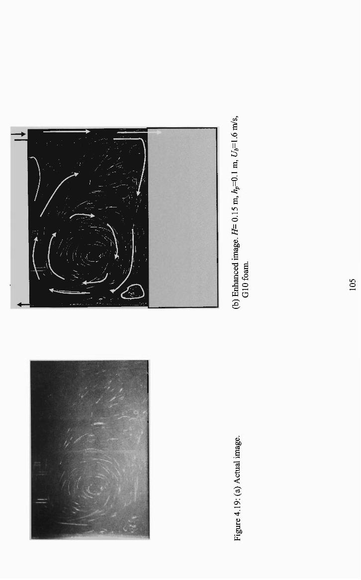
II
o II ^^ B
in
B • rH
73 a CO
c2
-§2 in
o
0) DO CO
B •1-H
a
OS
ii
I •1-H

o
DO CO
B "co
a <
o CN ^' ii
• ^H

•a.
in
o
o
ii
B 73 ii o
CO
c2
1 -
ii
B •1 -H
"cO
a < 'c?
CN

^ ^
0.68 0.04 0.06 0.08 0.10
Hm 0.12 0.14 0.16
Figure 4.22: Change in the radial position ofthe centre of re-circulation as a function ofthe fluid height for cases without foam.
0.40
0.10 0.04 0.06 0.08 0.10
Hm 0.12 0.14 0.16
Figure 4.23: Change m the radial position ofthe centie ofthe dominant re-circulation as a function ofthe fluid height for GIO foam with hp=0.05 m.
108

Chapter 5
Numerical simulations 5.1 Introduction
The numerical code that was validated against a benchmark natiiral convection
problem in chapter three was written for two-dimensional problems formulated in
cartesian co-ordinates. However, the experiments described in chapters four and six
were carried out in a system that was essentially axi-symmetiic. The code was
therefore modified so that it concurs with this geometry. Additional terms were also
included in the code to account for the presence of the porous foam used in the
experiments. This chapter describes these modifications and the application of the
modified code for simulating the experiments of chapter four.
Relatively few attempts have been made to model turbulent flow in porous
media as noted in a recent paper by Netto and Guthrie (2000). One reason for tiie
problem is the lack of experimental data that could be used to model such flows.
However, a more serious drawback lies in formulating the goveming equations, as
discussed in Sections 2.2.3 and 2.4.2 of chapter two. The Brinkman Forchheimer
extended Darcy (BFD) flow model (Equation (2.21)) has been used successfully by
authors such as Beckermann et al. (1988), Chen and Chen (1992), Song and Viskanta
(1994) and Chen et al. (1998) to simulate flow in porous media where inertial effects
become important but turbulence effects can be neglected. As described in Section
2.2.3.3 of chapter two, the BFD model also allows the numerical tieatment of a
composite system, such as that ofthe present study, as a continuum.
The development of turbulence models of flow within a porous medium was
necessitated due to their potential applications in the simulation of metal solidification
(Prescott and Incropera, 1995), modelling of turbulent combustion in porous burners
(Hall and Hiatt, 1996) and modelling of tiansport processes in stored produce (Chen
and Li, 1998), among others. As mentioned in Section 2.4.2 of chapter two, the
derivation of a turbulence model for flow in a porous medium within the framework
of the k-e model, involves the time averaging of the volume averaged BFD model
giving rise to a macroscopic turbulence model for the porous medium. Additional
109

terms in the k and e equations arise which are the product of the Darcy and
Forchheimer terms in the momentum equations. Depending on the characteristics of
the flow and the porous medium, these additional terms may either damp or aid
turbulence. Such a model was formally derived by Antohe and Lage (1997), although
authors such as Lee and Howell (1987) and Prescott and hicropera (1995) had
previously used modified forms of the k-e model to account for turbulence effects in
the porous medium in their simulations. These modifications were carried out in an
ad hoc manner, and little or no comparison with experimental results was presented
for the simulations performed with these models. For example, Prescott and
Incropera (1995) studied the effect of turbulence on solidification in a binary metal
alloy (the solidified region is treated as a porous mushy zone for the simulations) only
by comparing the predictions based on a low-Reynolds number k-e turbulence model
with those obtained with a laminar model. Chen et al (1998) showed through
simulations in the turbulent natural convection regime that turbulence in an adjacent
fluid layer does not penetiate the porous medium for a relatively low permeability
\K = O{l0~^j\. These authors used a simplified form ofthe turbulence model
developed by Antohe and Lage (1997) for flow in the porous medium. Netto and
Guthrie (2000) used a low-Reynolds number ^-f model and an ad hoc viscosity model
where the molecular viscosity was boosted 100 times to represent turbulence in a
model porous medium. Using a semi-analytical solution to validate the simulations,
these authors demonstrated the superiority of the results obtained with the low-
Reynolds number k-e turbulence model. However, no comparisons with experimental
results were provided.
The issue of turbulence modelling in a porous medium has been addressed in
die present research by comparing the results obtained from simulations with flow
visualisation and LDV measurements. As seen in the previous chapter, the
experiments involved a two-layer system consisting of a turbulent fluid layer
overlying a porous foam layer. The main problem in conducting experiments that are
useful for validation of a macroscopic turbulence model for the porous medium is the
difficulty in measurements or visualisations within the porous medium. In this work,
the issue is addressed by observing the changes in the flow field of a turbulent fluid
that is adjacent to porous media that have a range of permeabilities. The interaction
110

between the fluid and porous medium is enhanced by directing a jet of fluid into the
medium. Consequently, the egress of the fluid from the porous medium could be
closely observed.
5.2 Governing equations
Before formally presenting the goveming equations for axi-symmetric flow,
turbulence models of impinging round jet flows are briefly evaluated, because the
experiments use an impinging round water jet for generating turbulence.
5.2.1 Evaluation of turbulence models for impinging jet studies
It is well established from studies on impinging round jets (Graham and
Bremhorst, 1993; Craft et al, 1993; Durbin, 1996 and Behnia et al, 1999) that tiie k-e
turbulence model predicts higher than expected levels of turbulence in the stagnation
region. Craft et al. (1993) have argued that this stagnation point anomaly can be
attributed to the eddy-viscosity formulation, Equation (2.26), which is used to
represent normal stresses, for example:
v ' = - A : - 2 v , — (5.1) 3 '^y
In the irrotational region close to the stagnation point, tiie above relationship
—i—r 3w. leads to a turbulence kinetic energy generation rate, P^ = -u,u, —^, of:
ax.
Pk=^y, ^avV
(5.2) K^yj
With an increase in the turbulence energy, the value of v, increases, which in tum
leads to an increase in k.
Several modifications have been suggested to overcome this problem.
Changing the value of the constant Cei (Equation (2.35)) from 1.44 to 1.6, (Pope,
1978 and Graham and Bremhorst, 1993), gives rise to an increase in the rate of
dissipation of turbulence kinetic energy, e, thus reducing k. Authors such as Menter
(1992) addressed die problem from a more fundamental point of view by using a k-co
111

model instead of a A;-f model, which prevents an anomalous growth in k. However, as
pointed out by Durbin (1996), these modifications cause an anomalous growtii of
turbulence kinetic energy in rotating and swirling flows.
The Reynolds stress model used by Craft et al. (1993) and the elliptic
relaxation turbulence model (v^-/model) used by Behnia et al. (1999) seem to be tiie
only two models which have been validated for impinging round jet flows with heat
transfer. However, in the present study, the A:-e model is retained for computations for
the following reasons:
1) Since the system being considered is isothermal, heat tiansfer predictions that
greatly depend on the turbulence model used is not an issue.
2) The stagnation region is not of particular interest in the present study. It has been
found from preliminary computations that the mean flow pattems are well
represented by the A-f model.
3) For the porous medium, a modified form of the k-e model has been used. Thus,
when simulating systems that contain porous foam, it is suitable to use the k-e
turbulence model in the fluid layer in conjunction with the modified k-e
turbulence model for foam.
Three different versions of the k-e turbulence model were investigated for the
present simulations. These are discussed briefly below.
As described in Section 2.4.1.1.1 of chapter two, tiie standard /:-£• turbulence
model uses a wall function to represent the velocity profile close to the wall (Equation
(2.38)). The wall function was developed from experiments in a fully developed pipe
flow with favourable or negative pressure gradient. Since many flows are not as
simple as a pipe flow, low Reynolds number models (Section 2.4.1.2 of chapter two),
which solve for velocities and turbulent quantities right up to the wall were
developed. In order to account for the no-slip wall boundary condition, the low
Reynolds number models incorporated either a wall damping effect or a direct effect
112

of molecular viscosity, or both, on the empirical constants and functions in the
turbulence transport equations.
Since the present experiment has a flow that is significantly more complicated
than pipe flow, the wall fiinction approach is not suitable. Therefore, the standard k-e
turbulence model was used without wall fimctions for the mean velocities, similar to
the computations involving turbulent natural convection (Section 3.4.2 in chapter
three). With this model, the following values were assigned to k and e at the first inner
grid point. The expressions in Equation (5.3) are obtained from the inertial law
(details can be found in Section 2.4.1.1.1 of chapter two):
k^^jL,e = -L (5.3) c, /Of
The above form ofthe ^-£-turbulence model has been used in Henkes (1990),
Lankhorst (1991) and the present study for studying natural convection flows, because
the usual wall functions that apply in the case of simple forced convection flows do
not apply to natural convection flows. This approach can be considered to be a hybrid
of the standard k-e model (due to the use of wall functions for k and e) and the low
Reynolds number models (due to the practice of solving for mean velocities right up
to the wall).
hiitial computations using this approach were promising and led to convergent
solutions with relative ease. The use of wall functions for k and e at the first inner
grid point is akin to assigning a guess of these quantities. Thus, it was found that an
explicit specification for k and e at the jet exit is unnecessary for this case. However,
on grid refinement, the value of e showed an unbounded increase although the
solution converged in all cases. This approach was therefore deemed to be unsuitable
for further computations.
The low Reynolds number tiirbulence model originally proposed by Jones and
Launder (1972) (tiie low-Re tiirbulence model with code JL in Table 2.1) was used for
fiirther computations, histead of solving for the rate of energy dissipation e, it was
proposed by Jones and Launder (1972) to solve for the pseudo energy dissipation, ^ ,
where
113

« = ? + £> (5.4)
with D = 2v V ^^ J
This specification leads to the boundary condition 'e =0 at the wall. With k=0
at the wall, the boundary conditions can be specified convenientiy. However, in the
present computations, these boundary conditions gave rise to divergence. As shown
by Patel et al. (1985), the value of £ varies rapidly near the wall as compared to k and
the mean velocities. This rapid growth in 1 can be resolved only if one has
sufficientiy fine grids close to the wall. Therefore, it was decided to use a boundary
de condition of — = 0 (where x is normal to the wall), for the rate of energy dissipation
dx
as suggested by Patel et al. (1985) in connection with the original Jones and Launder
(1972) model. The wall value of e would then be a result ofthe computations. The
additional term in the turbulence kinetic energy equation, D (Equation (2.34)), and in
the energy dissipation rate equation, E (Equation (2.35)), would then vanish. Prescott
and Incropera (1995) have employed a similar approach in their computations.
5.2.2 Equations for axi-symmetric turbulent flow with modifications for flow
through porous media.
Having established the form of the k-e turbulence model to be used for the
impinging jet calculations, the goveming equations for the axi-symmetric system in
cylindrical co-ordinates are presented with modifications to account for flow through
porous media. The macroscopic turbulence model of Antohe and Lage (1997) has
been used as the basis for all turbulent flow calculations in the porous medium.
Therefore, tiiis model is introduced next in its entirety for an axi-symmetiic,
incompressible and isothermal system for steady state calculations.
1. Equation of continuity:
Z ^ K ) + ^ ^ 0 (5.5) r dr dz
114

Note that the x and ;; co-ordinates used for the two-dimensional cartesian equations in
chapter two are converted to tiie radial (r) and axial (z) co-ordinates for axi-symmetiic
calculations. The notation for the corresponding mean velocities have been changed
to Ur and Uz instead ofthe u and v velocities used earlier.
2. Momentum equation in the radial direction:
pu^ du^ pu^ du^ dp d
(j) dr (f) dz dr dr
a
(id ^
\r dr
+ -dz
P(hr K
(5.6)
fF</^rQ
Darcy term Forchheimer term
where Q = yju^ + ul .
Momentum equation in the axial direction:
(pJ + Pt)
du.
pu^ du^ pu,_ du^ _ dp I d
(j) dr (f> dz dz r dr ( du r
dr
d +—
dz {PJ + P\
P^,
dz (5.7)
.Q K 4K
Darcy term Forchheimer term
As mentioned in Section 2.2.3.3 of chapter two, the viscosity associated with the
Brinkman term, p^ - pJ, for the porous medium could have a value different from
title fluid viscosity. In the simulations presented in this thesis, the parameter J is
assigned a value of one so that the effective viscosity has a value equal to the fluid
viscosity. As discussed in Section 2.2.3.3 of chapter two, such an assumption has
some justification due to the analysis of Neale and Nader (1974). For the fluid layer,
die porosity, ^, is assigned a value of one in the momentum, k and e equations. The
Darcy and Forchheimer terms in the momentum equations vanish for the fluid layer
because the permeability, K, tends to infinity.
115

Note that the variables occurring in the momentum equations above have been
volume averaged first to obtain the BFD model (Equation (2.21)) and tiien time
averaged to exfract information about the turbulent quantities. The Forchheimer term
in the momentum equations was expanded by Antohe and Lage (1997) in their
Equation (4) before the time averaging process as:
1\I2 UjUj w. (uj+uj)(uj+uj)] («,+«:)
— , U,Ui
^Qu,-\-Qu,+-^—U:
(5.8)
Q
,1/2
where Q = (w w j in tensor notation.
These authors retained only the linear terms in the expansion and derived the
averaged momentum and turbulence transport equations. Recently Getachew et al.
(2000) used second-order terms in the expansion to arrive at extia terms in the
momentum and turbulence tiansport equations. Similar to the study of Antohe and
Lage, Getachew et al did not provide any numerical or experimental evidence to
support their model. Furthermore, the addition of fiirther higher order terms in the k
and e equations resulting from Getachew et a/.'s expansion lead to terms that is
extiemely difficult to implement numerically. Getachew et a/.'s model is not
employed for the present computations.
Turbulence kinetic energy equation:
pu^ dk pu^ dk
(f> dr ^ dz
d_
dr pj + Pt\dk_
^dr + -dz cr, dz + P -pJe-^pD
2(/>^k K
Darcy modification (DM)
8 j^pcp
3 ~J^{2Q)k v^
Forchheimer modification A (FMA)
c -1^-^Pt f - 1 du 2 du^ 2 du^ du^
UrK^-lT' + K - ^ + ^r -TT'^^z^r dr dz dr dz
(5.9)
Forchheimer modification B (FMB)
The above equation is the same as Equation (32) in Antohe and Lage (1997) written
for axi-symmetric systems in cylindrical co-ordinates.
116

Equation for the rate of energy dissipation:
pu^ de pu^ de _ d
<f> dr (j) dz dr pj^^
de
) dr + •
d_
dz pJ^tL de
e J dz
where
''(ceJA - pJc,J^e)j +pE
26-^—e
Darcy modification (DM)
d^dQ^ dk^dg dr dr dz dz
Forchheimer modification A (FMA)
+2(P ^
Apv,
d(uUd\\ u^ufd\ d\ dr
dz
Q[dr'
d(uUd'u^
-1-
+
2 . , A
Q
" . « z
+ -drdz dr^ + -Q
' d w.
drdz + JJ
(d\ d'u^ r +
Q\drdz] Q ydz" drdz] Q\dz + -ul (d'u
Forchheimer modification B (FMB)..
-1-2^ VZ
4 1 < p.v.
u. ^d\ d \ '
ydP '^drdz\ +
«.«z
V
(d\ d \ d \ d\^
dz' ^ dr'dz ^ drdz' ^ dr' +
u. d'u, d \
•+• y dz' dr^dz J
(5.10)
Forchheimer modification B (FMB) continued
Pk=P. (du.
dr + 2
(du.
dz + (du,. du.
''•+^^^1 + dz dr \r
(5.11)
u. Note that —^ in the production term, Pk, arises due to the co-ordinate
fransformation from two-dimensional plane to axi-symmetric cylindrical co-ordinates.
Pt =PcJu — (5.12)
117

k' and V = V T (^-^3)
The above equation is the same as Equation (33) in Antohe and Lage (1997) written
for axi-symmetric systems in cylindrical co-ordinates. The new constant c^* is
assumed to possess a value equal to Cp in the present simulations as suggested by
Lage (1998). The terms DM, FMA and FMB occurring in tiie A: and £ equations
vanish for the fluid layer because the permeability, K, tends to infinity for the fluid
layer. For simulations without foam, the extra terms in the momentum and turbulence
transport equations occurring due to the porous medium are dropped and the porosity,
, is set to unity.
From Equations (5.9) and (5.10), it can be seen that the DM term contiibutes
only towards damping turbulence. The Forchheimer modification terms could,
however, theoretically damp or aid turbulence depending on the sign of the velocity
components and their derivatives. As mentioned earlier, the terms in the k and e
equations (especially the FMB terms) are inconvenient to implement in a numerical
code even for the simple axi-symmetric geometry ofthe present problem.
As discussed in Section 5.2.1, a modified form ofthe low Reynolds number ^-£-model
of Jones and Launder (1972) is used for the simulations with the following constants
and parameters:
Cp=0.09, Cei=1.44, Ce2=1.92, CTk=I.O, cre=1.3
,fj=I.0,f2=I-0.3exp(-Re;), ( -2.5 ^
/ „ = exp ^ I + Re,/50 D=0. E = 0,
k^ where, 7? , = — . (5.14)
ve
5.2.3 Boundary and interface conditions
The following wall and symmetry boundary conditions were applied for
simulations without foam.
118

u,=u^=0
dx atr = i ? fo rO<z< / /
at 2 = 0 for 0 < r < /?
and atz = / f f o r O < r < ^ - H '
wall
du^ du, dz dz dk 3e _ dz dz
du^ _ ^"z _ Q
dr dr dk _de _^
atz = H for R-w<r<R
atz^H for R-w<r<R
atr = OforO<z<H
at r = 0 for 0 < z < 7/
^outflow (5.15)
•symmetry
dr dr
where R= radius ofthe cylinder=0.195 m, w is the width ofthe clearance (Figure 4.1),
and X is normal to the wall. Note that for the portion ofthe top wall, z = H, where the
fluid leaves the system through the clearance {R-w<r<R), axial gradient equal to
zero condition was applied for each variable. The same condition was also applied
for the symmetry line, at r = 0, with the radial gradient.
For the simulations with foam, laminar and turbulent flow models were used
for the porous foam. In these simulations, the low Reynolds number k-e model of
Jones and Launder (1972) was used still for the fluid layer. For calculations with a
laminar flow model for the foam, the interface between the porous medium and clear
fluid was treated like a solid wall for the turbulent quantities k and e. The motivation
for such a treatment of the system came from the visualisation experiments where it
was found that the fluid and porous layers could be regarded to be operating in the
turbulent and laminar regimes, respectively. This was found to be especially tme for
the low permeability foams that were investigated (Section 4.3.2.1 of chapter four).
de Thus, the interface conditions were given as k=0 and — = 0. The interface
dx
conditions for the velocities were satisfied automatically due to the use of the
Brinkman-extended Darcy flow model for the porous medium. Note that even with
tiie laminar flow model, inertial effects in the porous medium have been accounted
for, through the Forchheimer term in the momentum equation.
119

For calculations with a turbulent flow model for the foam, two sets of
simulations were carried out. In one set of simulations, only the Darcy damping or
DM terms in the k and e equations were retained, and the extra terms due to
Forchheimer modification were neglected (this set of simulations will henceforth be
referred as simulations with turbulence model TMl). An analogous approach was
adopted by Prescott and Incropera (1995) in their simulations of solidification of
metals where they assumed that, ""within a coherent mushy zone (model porous
medium), turbulence is dampened by shear having a characteristic length on the
order of dendrite arm spacings (i.e., by Darcy damping)". These authors used the
Darcy damping term only in the k equation without a similar term in the e equation.
In another set of simulations of the present study, the Darcy and Forchheimer
modification terms were retained in the k and e equations (this set of simulations will
henceforth be referred as simulations with turbulence model TM2). Of the two
Forchheimer modification terms FMA and FMB, only FMA has been retained for the
simulations, as justified in Section 5.4.2. In both sets of simulations, the equations
that govern the transport of k and e for the fluid layer and the porous medium were
solved without the need to explicitly account for the interface. Again, the use of the
Brinkman-extended Darcy flow model in the momentum equation in the porous
medium obviated the need to explicitly use an interface condition for velocities. The
boundary conditions were similar to the cases without foam.
5.2.3.1 Mean velocity at the exit of the jet
In the experiments corresponding to the present simulations, the pipe through
which the jet issues had a length of approximately 30 nozzle diameters. Craft et al.
(1993) have found that a pipe length of approximately 50 diameters can be considered
to give a fiilly developed flow at the exit of tiie jet. Baughn and Shimizu (1989) used
a longer pipe length of approximately 72 diameters. For the present investigation, the
region of interest is distant from the jet centieline. Preliminary computations witii a
fully developed profile at tiie exit of the jet, gave reasonable comparisons witii the
experimental results in the region of interest of the present study. Thus, one of the
profiles at die exit of the jet was chosen as a fully developed profile. Two different jet
120

exit profiles were specified in the present simulations, a flat profile corresponding to a
uniform (bulk, Ub) velocity at the jet exit and a fully developed velocity profile from
Bird e/a/. (1960), pg. 155,
(5.16) " z = "z.max
f l-
where u^
Uz,max
r
RN
Ut
1
r V -W "^,max 6 0 With — • — = —
R,) U, 49 = axial velocity.
= centreline axial velocity at the jet exit,
= radial location,
= radius ofthe nozzle and
= bulk fluid velocity.
Due to the use of a low Reynolds number turbulence model, some turbulence
had to be introduced into the system at the start. For the present simulations, this was
achieved by specifying values of A: and fat the exit of the jet (Graham and Bremhorst,
1993),
,,.-0.00117,
f,.., =0.1643 f k^s ^ (5.17)
III
y0.035Djj
The simulations with the two jet exit profiles are compared in Section 5.3.1.
5.3 Numerical methods
As mentioned earlier, the flow was assumed to be axi-symmetric for
computations. The flow pattems observed from the flow visualisation experiments
and an azimutiial fraverse carried out with the LDV probe confirmed the validity of
tills assumption. Thus, only one half of tiie actual flow domain needed to be solved.
A modified form of the finite volume staggered grid code (modified to include axi-
symmetric geometries) that was developed and validated for two-dimensional natural
convection flow problems (chapters two and tiiree) was used for all simulations. The
SIMPLE algoritimi detailed in Patankar (1980) was used for solving the discretised
partial differential equations using the control volume formulation. The hybrid, first
121

order upwind/second order cential difference scheme was used to discretise the
convection terms, whereas the diffusion terms were discretised using the second order
central difference scheme. A steady state approach was adopted for all computations.
To avoid divergence, an under-relaxation factor of 0.5 was employed for the mean
velocities and pressure, whereas for the turbulent quantities, k and e, the under-
relaxation factors were set to 0.3. All equations were solved in their dimensional
form.
The simulation was assumed to have reached a converged solution when the
sum of the normalised absolute mass and momentum sources (in the axial and radial
directions) for all control volumes was each less than or equal to 1x10"*.
Normalisation of the mass and momentum sources was carried out by dividing them
by the total number of control volumes (see Equation (2,72) for an example). Further
details about the SIMPLE algorithm and the discretisation procedure can be found in
the second chapter.
5.3.1 Grid generation and refinement
For grid refinement for the cases without foam, 100x100, 200x200 and
400x400 non-uniform grids were chosen for H=^0.15 m and hp-0.0 m (refer to Figure
4.1 for nomenclature). As an example of non-uniformity, with the 200x200 grid, 40
vertical grids were uniformly distributed horizontally in the jet region. Thus, 40 grids
covered a region equal to half tiie jet diameter, Dj, or 0.0095 m. Similarly, 20 vertical
uniform grids were distributed horizontally across the aimular clearance (Figure 4.1)
of width, w, 0.005 m. The remaining 140 vertical grids in the horizontal direction
were distributed non-uniformly by using the sine function given below in Equation
(5.18). All 200 horizontal grids in the vertical direction were distiibuted non-
uniformly by using the sine function given below in Equation (5.19).
rUr{i) = R sm i max 2n
2n-imax
zu,{j) = [H + hp) J a J sin\ 2K-
jmax 271 \ J max
I = I mm, I max
j = J mm, J max
(5.18)
(5.19)
122

The degree of non-uniformity of the grid generated by Equations (5.18) and
(5.19) can be controlled by assigning appropriate values to the variable a{0<a<]
with 0 representing a uniform grid distribution). In going from a uniform to a non
uniform grid distribution in the horizontal direction, the size of the contiol volume
should not change drastically, as it would lead to unrealistic solutions. In order to
avoid this problem, a was assigned a value of 0.6 in Equation (5.18) for
approximately matching the size of the control volume generated by the uniform grid
and the first control volume generated by the non-uniform grid. Similar grid
distributions were used for the 100x100 and 400x400 grids. Figure 5.1 shows the
200x200 non-uniform grid used for the computations for H=0.15 m and hp=0.0 m.
In Figure 5.2, the grid refinement study is illustrated for H=0.15 m and hp=0.0
m. In this figure, frames (a), (b) and (c) represent profiles for the radial velocity, axial
velocity and turbulence kinetic energy, respectively. In the figure, CFDFDP refers to
simulations carried out with a fully developed profile at the exit of the jet. The
profiles have been plotted at three non-dimensional axial locations {y/H locations)
which correspond to the locations where LDV measurements were made. As seen in
Figure 5.2, the results are grid dependent close to the wall at y/H=0.061. In going
from 100x100 grid to 200x200 grid, for example, the maximum variation in the radial
velocity is found to be around 15% based on the velocity obtained for tiie 200x200
grid aty//=0.067. However, the solutions become almost grid independent in going
from 200x200 to 400x400 grid. Therefore, the 200x200 grid was chosen for all
computations without foam with the same grid distribution as for H=0.15 m and
hp=0.05 m. Simulations carried out with a flat profile at the exit of tiie jet gave
similar grid independence.
For grid refinement for tiie cases with foam, 100x100, 200x200 and 400x400
grids were chosen for H=0A5 m and hp=0.05 m. The vertical grid distiibution in the
horizontal direction was maintained the same as in die cases without foam. The
interface between the foam and clear fluid was resolved by using closely spaced
horizontal grids in tiie vertical direction. This was achieved by using Equation (5.18)
in tiie fluid region as well as in tiie porous region and matching them at tiie interface
by using appropriate values of a. For the porous layer, a in Equation (5.19) was
123

assigned a value of 0.2 whereas for the fluid layer a value of 0.5 was assigned. For
200x200 grids, 100 grids were distiibuted in the fluid layer and 100 in the porous
layer. The chosen values of a resulted in similar grid sizes within the fluid and
porous layers close to the interface. The distance between two adjacent grids in the
vertical direction close to the interface was approximately 0.004 m. The resulting
grid for .^=0.15 m and hp=0.05 m is shown in Figure 5.3.
Figure 5.4 gives details ofthe grid refinement study carried out for H=0.15 m
and hp=0.05 m. In Figure 5.4, frames (a), (b) and (c) represent the radial velocity,
axial velocity and turbulence kinetic energy profiles, respectively. The normalised
axial positions have been maintained the same as in the cases without foam. The axial
velocity and turbulence kinetic energy profiles show little variation with grid
refinement from 100x100 to 400x400 grids. The maximum variation in the radial
velocity in frame (a) is again around 15%) based on the velocity obtained with the
200x200 grid (at y/H=0.061). The radial velocity profile becomes almost grid
independent in going from tiie 200x200 to 400x400 grid. Therefore, the 200x200 grid
was again chosen for computations for all cases with foam with the same grid
distribution as for H=0.15 m and hp=0.05 m.
124

Figure 5.1: Example ofthe non-uniform grid used for computations. H=0A5m, hp=0.0 m.
125
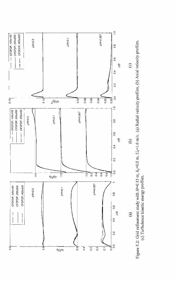
C3
Qn/n
P3 Ci II i
CO
CO
Ji
o
OH
'o
> "x <
CO
fB 2
'o _o 13 > 2 •3
CO
vo
::? 6 o o II
^ ^
S CO
m ia -^ tc o 2
4 ^
a "S CO C • . . . - <
si 2 -2
<7/7/n d d CO
d cvi d
r- O O d d
o CN in
U-,

Figure 5.3: Example ofthe non-uniform grid used for computations. H=0.\5 m. hp=0.05 m.
127

Qn/n
o o
o o ^ n n LL
n 11
o
o o il
o o CM
0. (J U-Q LL
o
o o -J o o • *
Q.
a LL Q U .
o
01
ci II
1
?
Q/7/n
ii o c Ji
-2 H
00
2 &,
+-»
'o
>
CO
2 'x <
CO
2
13 >
CO
1?
::D
B i n o o 11
tt.
-s: 6
i n
o
4
wit
h
>-.
tiid
VJ - 4 — »
c
fine
me
rid
O '^ i n
a l-l
a •1-H IUH
B a c2 o
O
s w
it
(U
ofil
l-l
cx >^
ener
g
u '+-' c
M
oo (N

5.4 Results and discussion
To evaluate the performance ofthe CFD simulations for the two-layer system,
comparisons have been made between the predicted results and the flow visualisation
experiments.
5.4.1 Simulations without foam
Simulations without foam are presented in Figure 5.5 for the three fluid
heights, H=0.15, 0.1 and 0.05 m in frames a, b and c, respectively. These frames
clearly show the single circulating cell for all three fluid heights as seen in the flow
visualisation experiments in Figures 4.4, 4.5 and 4.6. Thus, the CFD model is able to
predict the gross flow pattem for the cases without foam quite reasonably.
5.4.2 Simulations with foam
For simulations with turbulence model TM2, preliminary computations were
carried out, in order to evaluate the significance of the higher order FMB terms
(Equations (5.9) and (5.10)). For these computations, the new constant c* (Equation
(5.13)) was taken to be the same as Cp = 0.09 as suggested by Lage (1999). These
computations did not, however, lead to a converged solution even with a reduction in
the under-relaxation factor. The under-relaxation factors were reduced from 0.5 to
0.1 for the mean velocities and from 0.5 to 0.3 for k and e. The residual for the e
equation in these computations blew up indicating that the extra terms in the e
equation intioduced due to the Forchheimer modification could be causing the
problem.
hi order to understand the significance of the FMB terms, therefore, a new
sfrategy was adopted. Since the FMB terms in the e equation were potentially causing
problems with convergence, these terms were ignored for further computations. Thus,
tiie FMB terms were used only in the k equation. Other terms were used in their
original form. It was decided to compare the results obtained from these
computations with the results obtained without the inclusion of the FMB terms in
129

either the ^ or f equations. Such a comparison exercise should give an idea about the
significance ofthe FMB terms.
The simulations with the FMB terms only in the k equation converged.
Furthermore, the results with and without the FMB terms in the k equation were
almost identical with little change in any variable. As an example, the contours of
kinetic energy have been compared for the case of the highest investigated
permeability GIO foam in Figure 5.6. Frames (a) and (b) in Figure 5.6 represent
contours obtained with and without the FMB terms in the k equation for //=0.15 m,
hp=0.05 m and 17/,=1.6 m/s. It is clear from Figure 5.6 that the FMB terms have little
influence on the turbulence kinetic energy profiles. Similar results were obtained for
the other variables as well. Since the FMB terms in the k equation have negligible
influence on the final solution, it was decided to neglect this term for further
evaluation. The FMA tenn(s) are therefore the only Forchheimer modification terms
used in the k and e equations for further simulations with turbulence model TM2.
The gross flow pattems with the laminar flow model and with turbulence
model TM2 for the porous medium were found to be almost identical. The following
figures illustrate the reason for such a result. Figures 5.7, 5.8 and 5.9 give a
comparison between the contours of turbulence kinetic energy, rate of energy
dissipation and eddy viscosity, respectively, obtained with the two different
tiirbulence models for the GIO foam for H=0.15, 0.1 and 0.05 m with hp=0.05 m. In
the figure, the dashed lines indicate contours obtained with tiirbulence model TMl
and the solid lines indicate contours obtained with turbulence model TM2 for flow in
the porous foam. As seen from these figures, turbulence is damped almost completely
at the interface between the fluid layer and the porous foam with turbulence model
TM2. Thus, tile flow in the porous foam is effectively laminar even for the highest
permeability GIO foam due to the damping effect ofthe Darcy and Forchheimer terms
in turbulence model TM2. With ttirbulence model TMl, however, the ttirbulence
penetiates the porous foam to some extent. The eddy viscosity contours with
turbulence model TMl (contours represented by dashed lines in Figure 5.9) seem to
be anomalous due to their relatively large values in the porous foam. This anomaly
can, however, be explained by tiie fact that in tiie porous foam values of k and e are
almost negligible with the value of e being much smaller than that of k. Since the
130

k^ eddy viscosity is defined as, //, = pc — , it tends to give an artificially large value
e
even in regions where turbulence is almost non-existent.
Due to the similarity in the flow pattems obtained with the laminar flow model
and turbulence model TM2, the remaining results presented in the present chapter are
only with the two different turbulent flow models for the porous foam. The
comparisons are detailed below in the form of the effect of porous layer and its
permeability, effect of height/thickness ofthe porous layer and the effect of clear fluid
layer height. The flow visualisation experiments have shown that for the G30 and
G60 foams, the flow pattem in the fluid layer is not significantiy different. Thus, for
simulations with a lower permeability foam, the parameters for the G45 foam (see
Tables 4.1 and 4.2) of Seguin et al. (1998a) have been used, as the values for the G30
and G60 foams were unavailable from literature. The values reported by Seguin et al.
(1998a) for the Gl 0 foam are used in the present study.
5.4.2.1 The effect of porous layer and its permeability
The simulations carried out with the GIO and G45 foams give impressions
about the variation in flow pattem with a change in the permeability of the porous
foam. Figures 5.10 and 5.11 for the G45 foam and Figures 5.14 and 5.15 for the GIO
foam are used to study the effect of permeability of the porous foam to correspond to
the observations made in the flow visualisation experiments in Section 4.3.2.1 of
chapter four. Figures 5.10 and 5.11, and 5.14 and 5.15, respectively represent
simulations carried out with two different turbulence models, TMl and TM2, for the
porous foam with hp=0.05 m. Frames (a), (b) and (c) in these figures represent
simulations carried out for H=0.15, 0.1 and 0.05 m.
For the G45 foam, the flow in the fluid layer is similar to cases without foam
for H=0.15 and 0.1 m with botii turbulence models as seen from frames (a) and (b) of
Figures 5.10 and 5.11, respectively. This result is in agreement with the observations
made from tiie flow visualisations for low permeability porous foams in Figures 4.7
and 4.8 for tiie G60 foam and Figures 4.10 and 4.11 for the G30 foam. However, for
i/=0.05 m, die flow pattem in tiie fluid layer is significantly different with models
TMl and TM2 as seen from frame (c) in Figures 5.10 and 5.11. In Figure 5.10(c),
131

with model TMl, there is sufficient evidence ofthe formation of a second cell close to
the wall. This result is in agreement with the flow visualisation experiments for the
G60 and G30 foams as seen from Figures 4.9 and 4.12, respectively. In Figure
5.11(c), with model TM2, the second cell is not sufficiently developed, and there is no
significant change in the flow pattem in the fluid layer from cases without foam. This
result indicates that the additional Forchheimer terms intioduced in the k and e
equations might be providing excessive damping. This damping reduces the speed of
fluid leaving the porous foam, thus reducing its interaction with the flow in the fluid
layer.
For the GIO foam, for the two higher fluid heights, a two-cell pattem is
produced with both turbulence models for foam as seen from frames (a) and (b) of
Figures 5.14 and 5.15. There is, however, some difference in the size and shape of
the two cells simulated with the two models. In the corresponding visualisations for
the GIO foam in Figure 4.16, the two-cell pattem is not clearly formed for//=0.15 m.
This discrepancy could be due to the fact that the flow has unsteady and/or three-
dimensional characteristics, which the model does not take into account. However,
the two cell pattem can be clearly visualised for //=0.1 m in Figure 4.17. For H=0.05
m, the two simulations predict significantly different flow pattems as seen from
Figures 5.14(c) and 5.15(c). In Figure 5.14(c), for model TMl, the two-cell pattem
observed for H=0.15 and 0.1 m persists. This result is in agreement with the
corresponding flow visualisation in Figure 4.18. hi Figure 5.15(c), for model TM2
however, there is no evidence of the second cell, which again demonstrates the
inferiority of turbulence model TM2.
Similar conclusions can be drawn from the results obtained with two layers of
porous foam given in Figures 5.12 and 5.13 with the G45 foam and 5.16 and 5.17
with the GIO foam.
The above results indicate that turbulence model TMl is superior in predicting
tiie effect of porous layer and its permeability. Turbulence model TM2 provides
excessive damping due to the combined damping effect ofthe Darcy and Forchheimer
terms. As mentioned earlier, results obtained with a laminar flow model and
tiirbulence model TM2 for the porous foam were found to be similar.
132

5.4.2.2 The effect of height/thickness ofthe porous layer
For the lower permeability G45 foam. Figures 5.10 and 5.12 using model TMl
and Figures 5.11 and 5.13 using model TM2 are compared for the effect of
height/thickness ofthe porous layer. Figures 5.12 and 5.13 represent simulations with
G45 foam with Ap=0.1 m and correspond to Figures 5.10 and 5.11 with hp=0.05 m. A
comparison between frames (a), (b) and (c) of Figures 5.10 and 5.11 with the
corresponding frames in Figures 5.12 and 5.13 respectively, reveal that there is no
significant change in the flow pattem with a change in the thickness of the porous
layer. The flow visualisations for the low permeability G30 foam given in Figures
4.10 to 4.12 for hp=0.05 m and Figures 4.13 to 4.15 for hp=0.l m also showed no
significant change in the flow pattem in the fluid layer with a change in the thickness
ofthe porous foam.
For the highest permeability GIO foam, Figures 5.14 and 5.16 using model
TMl and Figures 5.15 and 5.17 using model TM2 are compared for the effect of
height^thickness ofthe porous layer. Figures 5.16 and 5.17 represent simulations with
hp=OA m and correspond to Figures 5.14 and 5.15 with hp=0.05 m. With model TMl,
Figures 5.14 and 5.16, there is a significant change in the flow pattern in the fluid
layer for //=0.05 m as seen from a comparison between frame (c) in these figures.
The two-cell pattem seen for hp=0.05 m in Figure 5.14(c) is reduced to a single cell
pattem for hp=0.l m in Figure 5.16(c). However, the flow pattem remains essentially
the same for H=0A5 and 0.1 m. With model TM2, Figures 5.15 and 5.17, the flow
pattem in the fluid layer is almost unchanged with a change in the thickness of the
porous layer for all three fluid heights. The flow visualisation results discussed in
Section 4.3.2.2 of chapter four, however, clearly indicate a delay in the transition to a
two-cell pattem in the fluid layer with an increase in the thickness ofthe porous layer
for the GIO foam.
The above discussion shows that simulations are not able to effectively
capture changes in the flow pattem in the fluid layer with a change in the thickness of
133

the porous layer. This result was found to be tme for simulations witii all three
models used for the porous foam.
5.4.2.3 The effect of clear fluid layer height
For the lower permeability foams, the effect of height ofthe clear fluid layer is
investigated by comparing individual frames of Figures 5.10 and 5.11 (which use
models TMl and TM2, respectively) for the G45 foam with Figures 4.7 to 4.9 ofthe
G60 foam or Figures 4.10 to 4.12 ofthe G30 foam. It is clear from the observations
made in Section 4.3.2.3 of chapter four that the flow pattem in the fluid layer is
essentially a single cell pattem for H=0A5 and 0.1 m for the G60 foam, Figures 4.7
and 4.8 and for the G30 foam. Figures 4.10 and 4.11. This result is predicted
accurately by model TMl, Figures 5.10(a) and (b), and model TM2, Figures 5.11(a)
and (b). For H=0.05 m, however, the flow pattem changes to a two cell pattem in the
visualisations for the lower permeability foams, as seen in Figures 4.9 and 4.12. This
result is predicted accurately only by simulations with model TMl for the porous
foam, as seen from Figure 5.10(c). Simulations with model TM2, on the other hand,
predicts only a single cell pattem for this case, as seen in Figure 5.11(c).
With the highest permeability GIO foam, the visualisations indicate a two-cell
pattem for all three fluid heights investigated for hp=0.05 m (Figures 4.16 to 4.18).
However, for H=0.15 m, the second cell is not completely formed. Figure 4.16.
Simulations with model TMl for the same case, Figure 5.14, show good agreement
for all three fluid heights with one dominant re-circulation close to the jet and a
second weaker cell close to the wall. Results with model TM2 are also comparable
with the visualisations for .^=0.15 and 0.1 m, as seen from Figures 5.15(a) and (b).
For H=0.05 m, however, the simulations are unable to predict the second cell close to
the wall, as seen from Figure 5.15(c).
The above discussion indicates that simulations with turbulence model TMl
are superior in their ability to predict changes in the flow pattem with a change in the
height ofthe fluid layer.
134

5.5 Conclusions
Simulations of a system consisting of a turbulent fluid layer overlying a
porous medium are presented in this chapter. The results obtained are compared with
the flow pattems observed through the flow visualisation experiments presented in the
previous chapter. Three different flow models are used for the porous foam, a laminar
flow model and two turbulence models. One of the turbulence models with only
Darcy damping in the k and e equations is superior in predicting the gross flow
pattems, especially the effect of permeability of the porous foam and clear fluid layer
height. The higher order terms occurring in the k and e equations due to the
Forchheimer term were found to be negligible through the simulations with the
second turbulence model. This model with both Darcy and Forchheimer
modifications included in the k and e equations for the porous foam was found to be
similar to the laminar flow model in its predictive capabilities. The similarity in
predictions was found to be due to the almost complete damping of mrbulence at the
interface between the porous foam and clear fluid due to the Darcy and Forchheimer
terms. As a result, the flow in the porous foam becomes effectively laminar in nature.
None of the three models used to represent flow in the porous foam could adequately
predict the effect of changes in the thickness ofthe porous layer.
135

B o o
m o o
o
VO
B o o
II
o
vq
T
B o o
II
B in
d
i CO
to
O V-i
O O H
+-> 3 O
.CI
ii CO CO
o l-l
to C
_o
.2 S
. . - I CO
O O ii >
CO CD O CO
i3
CO OD
in in ii
» i - <
til

0.0865 0.0807 0.0749 0.0692 0.0634 0.0577 0.0519 0.0461 0.0404 0.0346 0.0288 0.0231 0.0173 0.0115 0.0058
r
k
0.0865 0.0808 0.0750 0.0692 0.0635 0.0577 0.0519 0.0462 0.0404 0.0346 0.0288 0.0231 0.0173 0.0115 0.0058
1 ,;B
(a) (b)
Figure 5.6: Turbulence kinetic energy contours for GIO foam with H=0.15 m, hp=0.05 m, Ub=l .6 m/s. a) with FMB terms included in the k equation, b) without FMB terms in the k equation. The figure indicates that the FMB terms have a very small contribution.
137

—«5^^»^^^^^g
^ ^ / ^ V ^ -
I) ^
/ )TO
x / U I ' / w
K(ft^^•^
• - V ^
i m ^ ^ P ^ S MiJifiiHi 1 . :^ _.— . Vymimw ) ^ ^ ^ ^ ^ ^ ^ = % / / / / /
/ / 7 1 1 y /
o
3
'S ^ '
m/s
vq
T ::^ TS c CO
B i n o d 11
B <n o
1 m
, c)
//=
0
o
4 y .^*S
Jli
e m .—' d 4 l-l
cS
tour
s rg
y co
n
u
neti
c en
:3 o 4)
3 X l H ;3
r^ i n
o H
1 i i^
^ - v
-*
odel
TM
6
tion!
CO
cr (U ^
T3
- i ^
g in
the
uidi
CO
>. in
g on
ly D
are
CO
CO C
_o .2 75
(Zl
with
xt c
•1-H
obta
CO l- l
onto
u
o
ndic
ate
CO U C •1-H
4 I | CO CO
Q
CO C O
£ eq
uati
an
d
+-<
CO C O
o 43
'mo
d
o l-l CO
Q
and:
l-l
For
chhe
ime
bO
usin
CO
C O . i - H .4—1 CO
3 S
ith s
i
^ T 3 (U C3 cO
.t-) . O o
tour
s
c o o ii 1o o
'O -o ;r; o 5 6 00 w
OO CI

A
. CO
—I c r
^^ O 0)
II '^ - ^
^ g^.S 1 3 4) CO C^ Co C3 ill o -^ <!
II *-• i i
o p <U
B o ^ —I W ) PL,
=> •§ C ^ O CO
E ^ .2 • § J2 ^ S 3 o S g
4 ^ '
^ .S ^
o o c o o c o
d
4 2"
x> o tzi t-i 3 O c o o
•T3 T3
CO
.--^ -ti CO CO aj CO o * 5
CO
_ (Zl g >-g
C ^3 ?3
^ '^ ;5 — lU J3 -o 'O *i M ;i3 O CO CO o C
cJo in
ON

CO
—I o
—I c r ii ii
•O CO
6'g 00 53 O
to 3 cr
CO
a
VO "2 -.C
II ,k-»
t3 "5
^ Q 6 ^ in 5
? -s sL CO / — s CO
H ' l
?i Bi
in u .—I c
d 3 ll:; o / — V CO
CO t - l
CO O
•1-H
13 O
B o Jo Q
§ (U
l-l
cS
l-l 3 O
3 O c o o
CO
o c O -.. O 13 >^.B
. ^_ , • ^ H
1 3 CO
W Q 6\ in
fc
ii
o l-l
o bO C
. . - I CO 3 t« C3 O
. . - I
CO
S . .—I
CO
Xi
1 3 <U C
•s * - > -D O GO O
•>->
C5 O
o ii CO O
.S c
•1-H ^ _ ,
—< lU 13 13 ;r3 O
9 6 C/3 w
O '0-

vq
T
in o
^^
in o
CO
3
a o a, a
s l-l
13 (U CO
3
S H o ;_ 13 O
o c <D
3
VO
^
in o
"5;
o 4 e
i n o d II
in
o CO
c2
3 o l-l o CI.
(Zl <U CO
CO O l- l
cS
a
a C3 VO
II ^
^ B
m o o II R,
"C
B i n i~-<
o II 4
w
O *-> o <u > 13 C CO CO
O CO l- l +-»
B CO 0) is C/2
o , i n
u
gur
b

C/3
s VO
II
^ B m o o II
Cl, «sr B
i n o o 4 o
^—^
to
VO ^ II
6 m q d II Ci. "S:
B —. o
4 x>
m/s
VO
II .-. b B m o o II = -« •
t m
o II 4 CO
CO
3 O l-l
o O I
ii
s l-l
^ 13 ii CO 3
( N
:§ H .«_, a 13 o 6 o c ii 3
3 H
s i n o o II ex
-s: S ^ m •^ a B CO
o C+H
CO
3 O t- i
o a -B ^ CO
<u CO CO
o <U
X -> l-l
o cS CO
^—» O & I
O .4-t
o ii >
13 c CO K
o CO
is B , S £ <i> a iJ ,o
(Zl '+-'
^
m <L> l-l
§3 fe

CO
d K VO
II <i
tzi
3 O l - l
o a <u s ^ o <+:;
-B (/3 3
.- f-"
^^
in
o d
4 o
a 13 O
4) O
g 3 I
oo
^ VO
^ II
B 1—(
d II V ~s;
6 , o
4 — x>
t/>
^ vq
II . ^
B 1 — <
o II
Cl,
-«
B m 1—1
o
^^
Cl,
-« .G •1-H
^ in ^ O
i c2
(Zl 3
2 O a
.rj
CO (L) CO CO O <U
J3 +-• l-l
o fii (Zl -> o
O I
l-l
o o >
1 3
§ CO
iJ
1 6 2^ '^ is ,o 00 ' -i
ts f - ^
i n ii
a • ^H fe
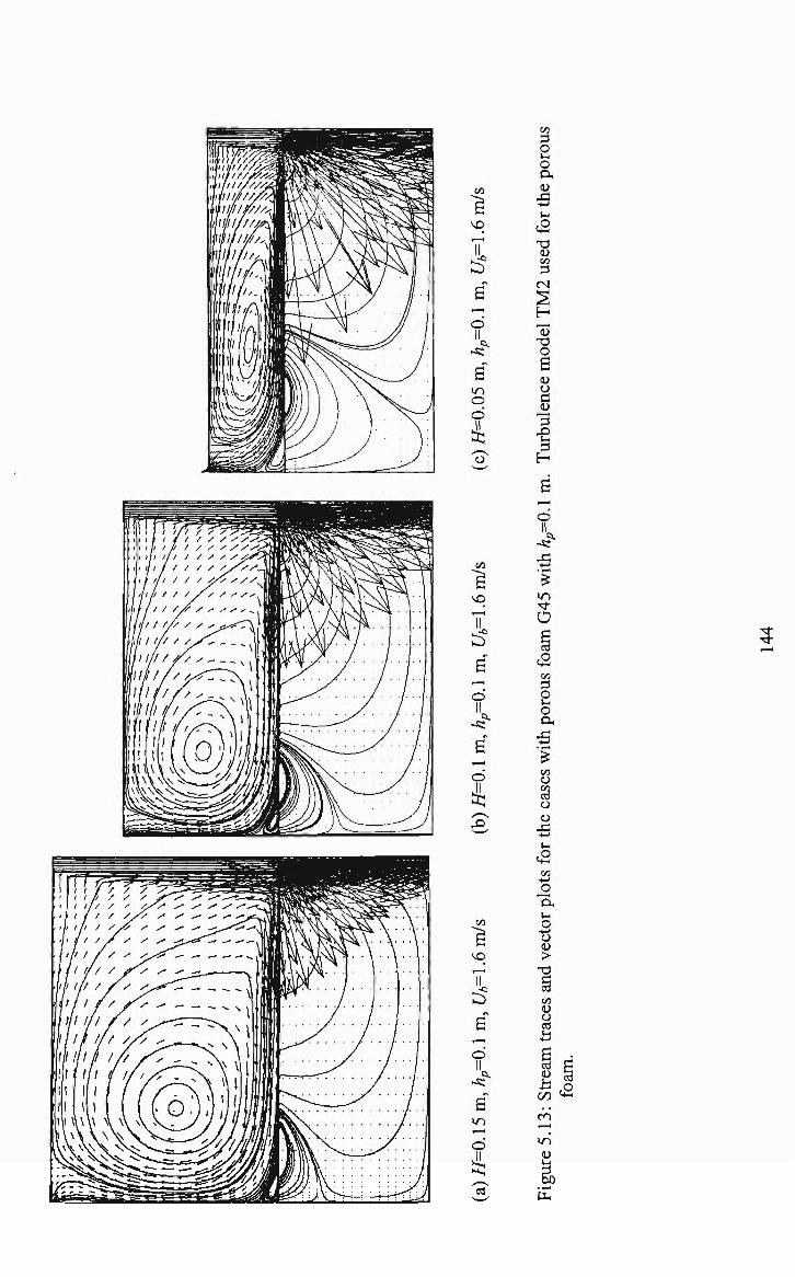
m/s
vq T t -
CO
3 O l-l
o D.
rtii
e
c2 13 4J CO
3
^^
in
o d 4
<N
13 O
ii O d
_4J
3 3
.. ^
VO
II ::? 6 .—* o II
> ^
i n ^f
o § cS
CO
3
oro
o-
d II
^ / N
.£>
M
^ VO t — (
II :D
B 1—<
o II
^^ •
d «n 1 ^ ^
o II '4 S3
CO
ii CO CO O
(U . d ^-' l-l
^ CO
+- I O O I l- l
O
a >
13
g oo (U o I i
^ - 1
g :
tiea
oam
00 ^
en •
i n
V
gur
f T .

CO
ri VO
T 1^ g
i n o o II
> ^
6 i n o o
CO
3 O l-l
o O I
ii
-4-t
i-t
c2 13
c« 3
S H ii
13 O 6 a o
ule
-P
VO
:^
i n
o d II
o
4 3~,
1 2 VO
:^
in
o
6 in
d 4
3
i n
o d II
o
a CO
c2
3 2 o CU
CO
<U (Zl CJJ O <U
• 4 - '
c2
O i
O o 4) >
13 C CO oo ii O CO l-l
<1 cS ^ c l
i n
I
i n

CO
^ VD . — 1
II b"
^ 6
t n o d II
^^
6 »n p d II tt;
/•^"N
o —'
oo
^ VO
II :^
B i n o o II
Cl.
-« 6
1—H
> O II
^ .£5
m/s
VO
II :^
^ a
i n o o II
Cl,
•.s;
6 m t—H
o II 4 CO
CO
cS CO 3 O l-l
o OH
4> .£3
i-l
c ^ 13 ,(D oo 3
t N
^ H ,_ 4> 13 O
B a o ri S 3
.o
F2 .
B i n o o
-«: J 3 + j
^ o 1 — *
O
§ cS tzi 3 O I H
o O I
rd •1-H
c« 4) 00 CO O 4)
.ri - 4 - ^ V H
c2 oo .*-! O CU t-l o o 4) >
1 3
§ CO 4) O CO
i3 ri c3 o i3
00
i n
, i n 4) «-i
IX,
VO

. VO
:^
(/3
3 O l - l
O CU ii ) - l
cS 13 4) t» 3
o .- II <u o.
-C
B i n o d 4 o
13 O B ii o ii
%i
% H
CO
g VO 1—H
II :^
g ,__,
• o II Cl.
~s;
B . — 1
o II 4
rC
(Zl
^ VO _ l
II l " B
. — 1
o II
t i .
"«; 6
i n
o II 4 CO
ti .
>« -fi
o 1 — 1
a
cS oo 3 O l-l
o CU
^ 00 ii CO CO O 4)
JS +-> l-l
o M H
oo *-" O CU V i
o •5 a >
-a U oo a o CO l-l
^-> B eS P <u a ^ ,o czi ^ VO
. i n
<u 5) fe
r-• ^

VO
1:5'
o
CO 3 O l-l
o O I ii
Si M-l
13 4) CO
3 CM
Cl. -s?
B i n r-) O
4
4) 13 O
6 4) O c & ^ • ^
X
H
o
CO
^ o ,__, II
;^ ^
6
o II Cl,
-.s:
6'" r-,
o II
4 Xl
tzi
^ VO
,_, II :5 B
i—i
o II
Q,
-«: B
i n • o II 4 CO
Cl,
-s; f i • ^
o t - H
O B CO
<B CO
3 O u O CU
^ ^ CO 4) CO CO O
ii .d .*-» l- l
o cii oo
^ . J
O CU l-l
o o ii >
13
g CO
oo ii O CO l- l
^-> B
& o * <
r-
m o
P->
CO

Chapter 6
LDV measurements and simulations 6.1 Introduction
This chapter presents laser Doppler velocimetry (LDV) measurements and
comparisons between CFD simulations and the measurements for the system
consisting of a turbulent fluid layer overlying a saturated porous foam. The
streaklines that were observed from the flow visualisations in chapter four,
highlighted the regions where more detailed experimental investigations were
required. Such detail has been achieved by taking LDV measurements. The
comparison of the simulations with the flow visualisations in chapter five was
qualitative in nature. A quantitative evaluation between the simulated and
experimental results is therefore presented in this chapter by comparing the CFD
simulations and the LDV measurements.
As noted in chapter four, few experiments have been carried out to evaluate
turbulence in porous media. Even the results firom the experiments that have been
performed cannot be used directly for a comparison with the simulations. The reason
is that the experimental results such as tiie ones by Hall and Hiatt (1996) and Saleh et
al (1992) give microscopic or pore scale values, whereas numerically, one is
calculating the macroscopic or volume averaged quantities. It has also been
recognised by authors such as Antohe and Lage (1997) that macroscopic tiirbulence
may persist only near the interface between a clear fluid and porous medium. Inside
the porous matiix, macroscopic turbulence may be attenuated rapidly since the large
eddies which tiansfer energy to the smaller eddies cannot be larger than tiie pore size
(Nield, 1991, and Nield and Bejan, 1992). For these reasons, the present experiment
uses a two-layer system consisting of a turbulent fluid overlying a porous medium and
infers tiie effect of tiie interaction between the two layers on die flow pattems in the
fluid layer.
As indicated in chapter four on flow visualisation, it was found tiiat there is a
significant change in the flow pattem in tiie fluid layer ofthe two-layer system when
die highest permeability (GIO) foam was tested. For the LDV measurements
149

therefore, only the cases with the GIO foam have been revisited. All cases without
foam were also repeated to ascertain the nature ofthe flow pattem.
Since the flow in the fluid layer is turbulent, it is expected that this turbulence
will persist, on the macroscopic scale, in the foam for some foam height before it is
attenuated. It is fiirther believed that a proper representation ofthe flow in the porous
medium will lead to a better prediction of the flow in the fluid layer due to the
interaction between the two layers. The CFD simulations presented in chapter five
revealed that the simulations with a turbulent flow model for the foam and only Darcy
damping incorporated in the k and e equations (referred as model TMl) gave better
predictions of the flow pattems in the fluid layer. Simulations witii a laminar flow
model and a turbulent flow model with Darcy and Forchheimer modification terms
incorporated in the k and e equations (referred as model TM2) gave identical results
for the flow pattems. These two models were inferior to model TMl in predicting the
effect of permeability of porous foam and clear fluid layer height on the flow pattems
in the fluid layer. In this chapter, these models are again compared for their ability to
quantitatively predict the mean velocity and turbulence kinetic energy pattems in the
fluid layer obtained fi*om LDV measurements.
6.2 Principles of LDV
LDV measurements have been carried out to record velocities and turbulence
intensities. The principle of this measurement technique has been described in detail
in Durst et a/. (1976). For completeness, a brief description of the technique is
presented here.
The LDV is based on the Doppler effect and can be operated in three different
optical arrangements, namely, the reference beam mode, the dual beam or fiinge
mode and tiie two-scattered beam mode (Durst et al, 1976). The present system uses
die fiinge mode of operation as illustiated in Figure 6.1. hi this mode, two incident
light beams of almost equal intensity intersect in space to create an interference
fringe. If a scattering particle penetiates the region of intersection of the two light
beams, it will scatter light fi-om each ofthe two beams. The scattered light waves thus
produced will have Doppler shifted frequencies given by the relationship:
150
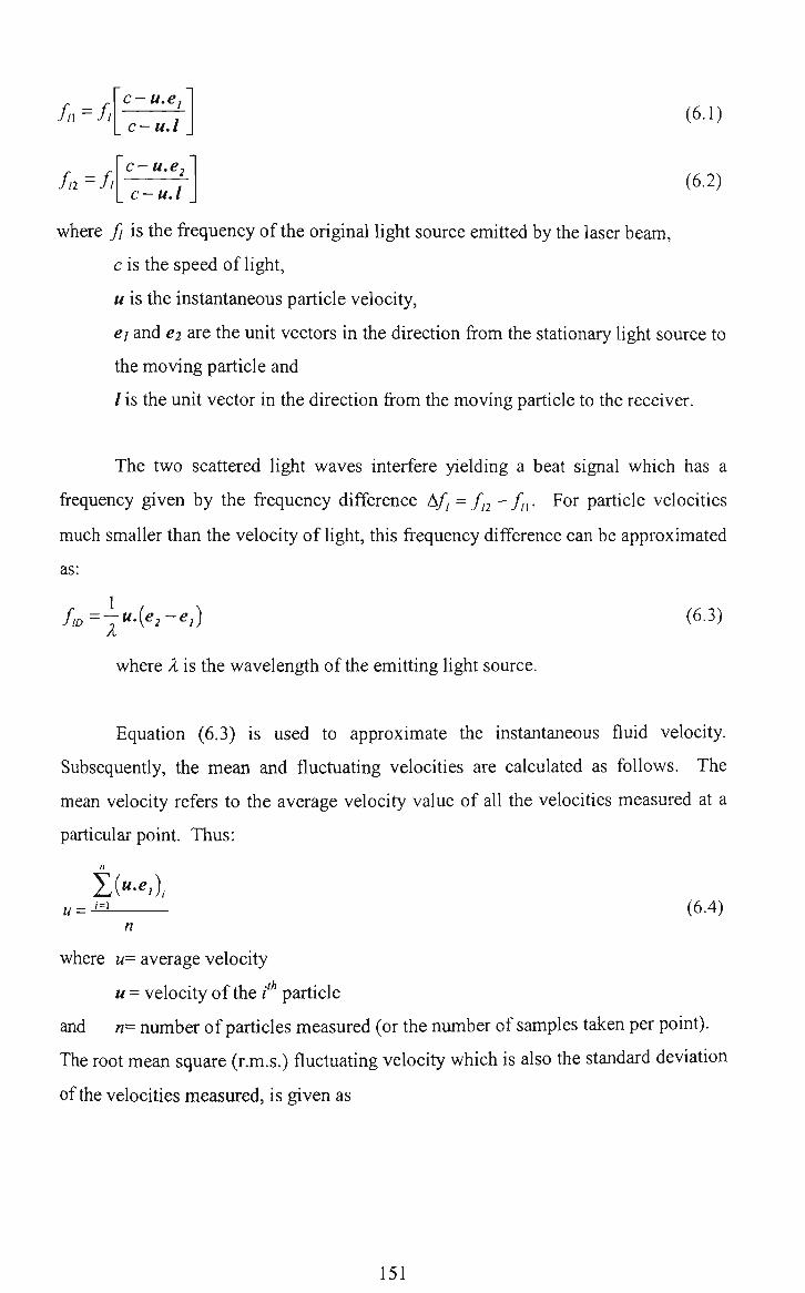
/ / •=/ /
fa ~ JI
C-U.Bi
c-u.l
c-u.e^ c-u.l
(6.1)
(6.2)
where // is the frequency ofthe original light source emitted by the laser beam,
c is the speed of light,
u is the instantaneous particle velocity,
ei and €2 are the unit vectors in the direction from the stationary light source to
the moving particle and
/ is the unit vector in the direction from the moving particle to the receiver.
The two scattered light waves interfere yielding a beat signal which has a
frequency given by the frequency difference A/) = f^^ - f^. For particle velocities
much smaller than the velocity of light, this frequency difference can be approximated
as:
fiD=jU.(e2-ej) (6.3)
where X is the wavelength ofthe emitting light source.
Equation (6.3) is used to approximate the instantaneous fluid velocity.
Subsequently, the mean and fluctuating velocities are calculated as follows. The
mean velocity refers to the average velocity value of all the velocities measured at a
particular point. Thus:
u = _ /=i (6.4)
n where w= average velocity
u = velocity of the / particle
and n= number of particles measured (or tiie number of samples taken per point).
The root mean square (r.m.s.) fluctuating velocity which is also the standard deviation
of die velocities measured, is given as
151

^ Z(«-^/-"),-u'=^^-^
n-l (6.5)
where Vw = the r.m.s. fluctuating velocity.
For all three optical arrangements mentioned above, the LDV can be operated
either in the forward scattering or backward scattering mode of operation.
Laser beam 2 Interference fringe
Laser beam 1
Figure 6.1: An illustiation ofthe LDV operating in the fiinge mode.
6.3 LDV setup, traversing mechanism and data acquisition
For the present experiments, the LDV is used in the backward scatter mode.
The LDV system was provided hy Aerometrics (1997). It consists ofthe LDV probe
and the DataVIEW software. The incoming beam has a wavelength of 514.5 nm. A
1 W Argon ion laser is used as the light source for the present experiments, and it is
connected to a fibre optic probe through a fibre optic cable. A Bragg cell is used as a
beam splitter and frequency shifter. Frequency shifting allows the 180 degree
152

ambiguity in the direction of the measured velocity to be resolved. The Bragg cell
splits the incoming beam into two beams of almost equal intensity (!5-10%). One
ofthe beams is shifted by a frequency of 40 MHz with respect to the frequency ofthe
incident beam. A single channel LDV acquisition system is used for the
measurements. Thus, only the normal Reynolds stresses and the mean velocities
could be determined.
A high sampling rate leads to an increase in the velocity range that can be
measured by the instmment, but decreases the signal quality. On the other hand, a
low sampling rate leads to a reduced velocity range that can be measured, but
increases the signal quality. Thus, the sampling rate was optimally adjusted to 10
MHz by a trial and error procedure, and a low pass filter of 5 MHz was applied
following the Nyquist criterion.
Figure 6.2 shows a photograph of the experimental setup used for the LDV
measurements. Measurements could not be taken closer than 0.015 m to the lower
wall and 0.01 m to the upper wall for the axial velocity due to the limitations
presented by the physical boundaries of the experimental setup. Since it was decided
to obtain vector plots by using the axial and radial velocities, the limits on the
measurements were set by the ability to measure the axial velocity. A simple
schematic diagram of the experimental setup is presented in Figure 6.3 illustiating the
tiaversing mechanism and the data acquisition system. The same impinging jet setup
as the one used for flow visualisation experiments presented in chapter four has been
used. As shown in Figure 6.3, the LDV probe was attached to a robotic arm. The
robotic arm served as the tiaversing mechanism.
Information about the measurement position was fed to the robot contioller
through tiie Lab View software (installed on a Pentium based personal computer,
PCI). The DataVIEW software (installed on a 486 personal computer, PC2) was
used to commimicate between the LDV system and die LabView software in PCI.
Once a measurement position was assigned to the robotic arm through Lab View, the
DataVIEW so^arQ was also activated to record measurements. The raw data along
witii tiie information about mean velocity (Equation (6.4)) and root mean square
153
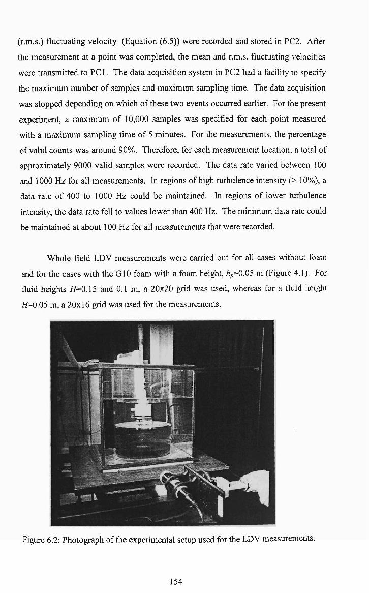
(r.m.s.) fluctuating velocity (Equation (6.5)) were recorded and stored in PC2. After
the measurement at a point was completed, the mean and r.m.s. fluctuating velocities
were transmitted to PCI. The data acquisition system in PC2 had a facility to specify
the maximum number of samples and maximum sampling time. The data acquisition
was stopped depending on which of these two events occurred earlier. For the present
experiment, a maximum of 10,000 samples was specified for each point measured
with a maximum sampling time of 5 minutes. For the measurements, the percentage
of valid counts was around 90%. Therefore, for each measurement location, a total of
approximately 9000 valid samples were recorded. The data rate varied between 100
and 1000 Hz for all measurements. In regions of high turbulence intensity (> 10%), a
data rate of 400 to 1000 Hz could be maintained. In regions of lower turbulence
intensity, the data rate fell to values lower than 400 Hz. The minimum data rate could
be maintained at about 100 Hz for all measurements that were recorded.
Whole field LDV measurements were carried out for all cases without foam
and for the cases with the GIO foam with a foam height, ^ ,=0.05 m (Figure 4.1). For
fluid heights H=0.15 and 0.1 m, a 20x20 grid was used, whereas for a fluid height
H=0.05 m, a 20x16 grid was used for the measurements.
Figure 6.2: Photograph of die experimental setup used for the LDV measurements.
154

To bottom tank
Water level •*-
From overhead tank
Experimental rig
1 LDV probe
Labview Software
•^i optic tibre
Robot Control
LDV system
Dataview Software
LASER
PCI
PC2
Figure 6.3: Schematic diagram ofthe experimental setup used for the LDV measurements.
6.4 Seeding particles for LDV measurements
Impurities present in tap water were first removed by passing it through a filter
(particulate reduction of 99.96% up to 1-2 pm particles). Finely ground pearl
particles, Magna Pearl (average size ~1 pm) supplied by Bronson and Jacobs, were
then added to the water as seeding particles. Trial mns were carried out to estimate
the optimum amount of seeding particles. It was found that after adding
approximately 1 g of seeding particles, the data rate in the majority of the measured
domain remained at or above 400 MHz. Additional seeding particles did not change
the data rate significantiy. Due to the presence of stagnant regions in the flow as the
fluid tiavelled from the bottom tank to the overhead tank and then into the
experimental rig, there was a reduction in the concentiation of the seeding particles in
die flow over a period of time (typically one hour). This reduction necessitated
additions of approximately 0.5 g of seeding particles per hour. The tank situated at a
lower level than the experimental rig (the bottom tank in Figure 6.3) acted as the
reservoir of water. Adding seeding particles to the bottom tank ensured that their
addition did not interfere with the flow in the experimental rig itself Typically,
155

around 5 hours were required to complete one mn of an experiment consisting of 400
data points, corresponding to 20x20 grids for H=0.15 m and 0.1 m.
6.5 Measurement considerations and error estimation
6.5.1 Uncertainty analysis
Using the repeatability of measurements, the uncertainty in the estimation of
the mean and fluctuating quantities was checked. In order to check for accuracy in
the entire flow domain (from regions of high turbulence intensity to regions of low
turbulence intensity), a total of five sweeps was employed in the radial direction to
measure the axial mean and r.m.s. velocities. The averaging time varied from 9s to
90s corresponding to data rates of 1000 Hz and 100 Hz, respectively. Figure 6.4
illustrates the repeatability measurements carried out for the mean and r.m.s axial
velocities. The mean velocity in Figure 6.4(a) shows considerable overlap among the
five different traverses, indicating good repeatability. The r.m.s velocity in Figure
6.4(b), on the other hand, shows a larger scatter. The uncertainty in the mean velocity
measurements was found to be within ±2%, and within ±10% in the r.m.s. velocity
measurements. The radial mean and r.m.s. velocities were found to have similar
repeatability results to the axial ones.
6.5.2 Positioning errors
The positioning error can be attributed to three factors:
1. Spatial accuracy ofthe tiaversing mechanism, in this case the robotic arm,
2. The non-cylindrical nature ofthe container and
3. Inaccuracy in the positioning of the nozzle of the j et exit.
The second and third errors are related, since an accurate positioning of the nozzle at
the geometrical centie of the container requires an apriori knowledge about the
centie.
156

The spatial accuracy of the traversing mechanism was found to be of the order
of ±10pm. The finite size of the measuring volume also contributed to the
positioning error. However, these errors were small in comparison with the error in
the positioning of the origin of each fraverse, corresponding to the cylinder centieline,
due to the noncircular cross-section of the cylinder. The origin for each tiaverse was
fixed by assuming the cylinder to have a perfectly circular cross-section. This is not
strictly the case because the cylinder was made of acrylic which is not a stmctural
material. For the measurements, it was also assumed that the centie of the jet
coincided with the centre of the cylinder. The position of the centre of the jet with
respect to the centre of the cylindrical tank has been estimated through measurements
as described in the next section.
1.0
0.9
0.8
0.7
0.6
0.5
0.4
0.3
0.2
0.1
0.0
-0.1
•
': ':
' •
•
; ;
• ;
%
:3^
0.0 0.2 0.4 0.6 r/R
0.8 1.0
0.20
0.18
0.16
0.14
0.12
0.10
0.08
0.06
0.04
0.02
0.00 0
i g 8 e S 8 » 8 i g 8 Bgi8j!
,0 0.2 0.4 0.6 0.8 1.0 r/R
(a) Axial mean velocity (b) Axial r.m.s. velocity
Figure 6.4: LDV measurements representing the magnitude of the uncertainty in the mean and r.m.s. velocities through repeatability tests. A total of five repetitions has been performed at each measurement location. Notice that for the axial velocity measurements in Figure 6.4(a), there is considerable overiap in tiie measurements indicating excellent repeatability.
6.5.3 Adjustinent for deviation of the centie of the jet from tiie centie of the tank
157

As mentioned in the previous section, the position of tiie centre of the jet (or
nozzle from which the jet issues) and the centie of the cylindrical tank might not be
aligned. In order to evaluate this error, a tiaverse was carried out through the tank
centreline for the case without foam with a fluid height / / = 0.15 m. hi Figures 6.5(a)
and 6.5(b), the axial mean and r.m.s. velocity measurements, respectively, are given
through the tank centreline at a height of z = 0.135 m from the tank base. As shoAvn
in these figures, there was a deviation of approximately 3 mm in the case of the axial
mean and r.m.s. velocities between the tank and jet centres. This deviation was
observed in all experiments that were conducted, and therefore, it can be considered
to be a systematic error. Since the origin for the traverses had already been fixed,
using the circular tank as the reference, it was decided to first take measurements
assuming the origin to be at the apparent tank centie. The results were then adjusted
by 3 mm to account for the misalignment.
6.5.4 Location of the measuring volume
The different refractive indices of the media through which the laser beams
pass before forming a measuring volume needed to be taken into account to calculate
the actual position at which the beams intersect (i.e., to calculate the location of the
measuring volume). Otherwise, a shift exists between the actual measuring volume
location and its apparent position in air. The information about the actual position
thus obtained was entered into the LabView software (see Section 6.3).
The actual location of the measuring volume was determined by performing a
beam path analysis using Autocad. Figure 6.6 illustiates an example ofthe beam path
analysis performed when the two beams are horizontally aligned. This is the case
when the radial mean and r.m.s. velocities have to be measured. The figure shows the
top view of the experimental setup. For axial velocity measurements, the two beams
would be aligned vertically.
One quarter of the acrylic cylindrical tank and the square glass tank is shown
in Figure 6.6. The distance from the LDV probe to the centieline ofthe cylindrical
tank is 558.05 mm, whereas the distance of tiie probe from the outer surface of the
square glass tank is 330.45 mm. The extemal half side length ofthe square glass tank
158

is 227.60 mm. These measurements are shown in Figure 6.6. For the analysis, the
curved side of the cylindrical tank is approximated as 0.05 degree facets. As a
reference for the analysis, the direction of the "Observer" is shown in the figure with
an arrow. X-X and Y-Y represent lines passing through the centieline of the
cylindrical tank. For all calculations, the refractive indices, RI, of water, air, acrylic
and glass are taken to be equal to 1.330, 1.000, 1.490 and 1.510, respectively. The
thickness ofthe square glass tank and the cylindrical acrylic tank are 12.6 and 5 mm,
respectively. The focal length of the beam and the beam separation are 500 and 40
mm, respectively. With these input parameters, the change in the path of the laser
beams due to the refractive index changes was calculated using Autocad.
It was decided to take into account the shift in the location of the measuring
volume only when it was greater than ±lmm. For the vertical beam alignment (axial
velocity measurements), the shift was never greater than 1 mm. Therefore, no
correction was made for axial velocity measurements.
For the horizontal beam alignment (radial velocity measurements) as shown in
Figure 6.6, the shift was found to be greater than 1 mm, but in the direction opposite
to that ofthe "Observer" for positions close to the centie ofthe cylindrical tank. For
example, in Figure 6.6, the shift in the location ofthe measuring volume is 1.318 mm
and in the direction opposite to that of the "Observer". As one goes away from the
centre, for the horizontal beam alignment, the shift first decreases and then increases
but towards the "Observer". In the case of positions at 175, 180, 185 and 190 mm
away from the centie of the tank, for which measurements were recorded, the shift in
the location of the measuring volume was found to be greater tiian 1 mm and in the
direction of the "Observer". Thus, in tiie case of the horizontal beam alignment, five
positions corresponding to the centie ofthe tank and 175, 180, 185 and 190 mm away
from the centie of the tank had to be corrected for tiie shift in the location of the
measuring volume. These positions and the corresponding shifts are presented in
Table 6.1.
159

1.8
1.2
0.8
0.4
0.0
-
-
•
•
1.. 1 1 . i.
(
•
•
1 1 _ l _ . 1. .
. • - . . •
•
>
1 1 1 1
• •
•
•
•
•
•
I I I !
z = 0.135m
-0.03 -0.02 -0.01 0.00 0.01 0.02 0.03 rva.
(a): Axial mean velocity profile through tank centreline. H=0.15 m, hp^O.O m, ^4=1.6 m/s
0.5
0.4
0.3
0.2
0.1
0.0
-
•
-
•
• (
•
•
1
•
• •
•
• • • • •
•
• •
• • •
•
z = 0.135 m
-0.03 -0.02 -0.01 0.00 rva.
0.01 0.02 0.03
(b): Axial rms velocity profile through tank centieline. H=0.15 m, hp=0.0 m, Ub=l.6 m/s
Figure 6.5: LDV measurements indicating tiie deviation of tiie centie of die jet from the centie of the tank.
160

1.318 beyond c/1
Beam crossing on c/1 Y-Y
5.00
558.05
Approximated by 0.05 degree
facet,"?
12.60
20.00
40.00
Figure 6.6: Horizontal beam analysis on centieline axis Y-Y. All measurements are in mm.
161

Table 6.1: Shift in the location of the measuring volume in case of tiie horizontal beam alignment (corresponding to the radial velocity measurements). The positive sign indicates that the apparent shift is away from the observer. The negative sign indicates that the shift is towards the observer. Figure 6.6 indicates the direction ofthe "Observer".
Position from centieline of tank
(mm) 0
175 180 185 190
Apparent shift in the position
(mm) +1.318 -2.813 -4.890 -6.686 -8.633
6.6 Numerical simulations
Details of the goveming equations used for the axi-symmetric system with a
fluid and porous layer, the boundary and interface conditions and the numerical
methods used can be found in chapter five, and they are not repeated here. In the next
section, the numerical results are compared quantitatively with the LDV
measurements.
6.7 Results and Discussion
6.7.1 Measurements and simulations without foam
As discussed earher, for the measurements, a 20x20 grid was used for H=0.15
and O.IO m, whereas a 20x16 grid was used for i7=0.05 m. The limits for
measurements were set by the ability to measure the axial velocity (see Section 6.3).
hi die results, comparison with the experimental vector plots and stieamtiaces give an
indication of the ability of the numerical model to predict tiie gross flow
characteristics. The profiles of mean axial and radial velocity as well as the
turbulence kinetic energy have also been compared to give a quantitative comparison
between the CFD simulations and LDV measurements.
162

6.7.1.1 Vector plots and streamtiaces
Figure 6.7 gives a comparison between the experimental and numerically
predicted vector plots. Frames (a), (c) and (e) are the experimental results, whereas
frames (b), (d) and (f) are the simulated results for H=0.15, 0.1 and 0.05 m,
respectively. The streamtiaces have been superimposed on the vector plots for
visualising the gross flow pattem. For all the heights considered, there is only a single
circulating cell occupying the flow domain. These results are in agreement with the
flow visualisations given in Figures 4.4, 4.5 and 4.6 of chapter four. The simulations
reproduce the single circulating cell, although the position of the cell is not predicted
accurately. This discrepancy could be because the actual flow can have unsteady
characteristics. It has been reported that impinging round jet flows in an enclosed
cylinder are toroidal (Ngamsirivadhana, 1996). The frequency of oscillations ofthe
cell depends on the aspect ratio and the jet velocity. However, for the present
simulations, this aspect of the flow has been ignored, and the flow is approximated to
be steady state.
The effect of decreasing liquid height on the horizontal position of the centre
of re-circulation for cases without foam is seen in Figure 6.8. The vertical axis, Rc/R,
represents the normalised radial position of the centre of the dominant re-circulation
from the centreline. The horizontal axis, H, represents the height ofthe fluid layer in
metres. Comparison of results is given in Figure 6.8 as obtained from the
visualisations, measurements and simulations. The LDV measurements and
visualisation results show a similar tiend. The centie of re-circulation moves closer to
die wall with a decreasing liquid height. However, the simulations indicate negligible
change in the position of the re-circulation with liquid height. As indicated above,
tills anomaly could be due to the fact that the flow has unsteady and/or three-
dimensional characteristics, which the model does not take into account.
163

(a) LDV measurements (b) CFD simulation H=0.15 m, hp=0.0 m, Ub=l.6 m/s
(c) LDV measurements (d) CFD simulation H=0.l m, hp^O.O m, Ub=l.6 m/s
(e) LDV measurements (f) CFD simulation H=0.05 m, hp^O.O m, ^^=1.6 m/s
Figure 6.7: Measurements and simulations for the cases without foam. Vector plots and stream traces.
164

^ <<
0.82
0.80
0.78 -
0.76 -
0.74 -
0.72
0.70
0.68
A
•
-
•
-
1
m
•
1 1 1
•
• •
Visuahsation Measurement Simulation
•
•
•
1
0.04 0.06 0.08 0.10
Hm
0.12 0.14 0.16
Figure 6.8: Change in the horizontal position ofthe centie of re-circulation as a function ofthe fluid height.
6.7.1.2 Mean axial velocity profiles
Figures 6.9, 6.10 and 6.11 show comparisons for the axial velocity profiles for
fluid heights of 0.15, 0.1 and 0.05 m, respectively. In these figures, the profiles have
been plotted for six different axial locations covering the entire measurement plane.
Frames (a) and (b) in each figure present comparisons when a flat profile (CFDFP)
and a fiilly developed profile (CFDFDP), respectively, are used in the predictions at
the exit of the jet. Also, in each figure, the effect of grid refinement has been shown.
A comparison between frames (a) and (b) in each figure shows firstly the
effect of the two profiles at the exit of the jet. It can be seen that botii profiles at the
jet exit fail to predict the flow close to the jet and in the region close to the jet
centieline. With both flat and fully developed profiles, the reduction in the centreline
velocity witii axial distance is under predicted. The reason is that the flow in die pipe
is still not fiilly developed, whereas the model assumes a fully developed or flat
profile. The actual profile close to the jet exit would be closer to a developing pipe
165

flow with turbulent boundary layer profiles at pipe walls in the present experiment.
With the specification of a flat profile, another problem is with the resolution of the
flow close to the jet exit. The sudden change from a flat velocity profile in the jet as it
enters the cylinder cannot be resolved numerically with any amount of grid
refinement. The resulting discontinuity in the axial velocity at r/R=0.03 and 0.04 for
/f=0.1 m and //=0.05 m {hp=^0.0 m), respectively, is shown in Figures 6.10(a) and
6.11(a). However, the axial velocity away from the jet centrehne is predicted well,
regardless ofthe profile at the exit ofthe jet indicating that the jet exit profile does not
play a significant role in determining the flow characteristics away from the jet
centreline. Since the region of interest for the present study, is distant from the
centreline of the jet, fiirther investigation on the profile at the exit of the jet was not
carried out. However, it is desirable to design future experiments ensuring a fiilly
developed profile at the exit of the jet. Overall, Figures 6.9 to 6.11 indicate
reasonable agreement between the measurements and simulations for the axial
velocity.
6.7.1.3 Mean radial velocity profiles
Figures 6.12, 6.13 and 6.14 give a comparison ofthe mean radial velocity
profiles. Here again, the frames (a) and (b) in each figure show comparisons made
with two different jet exit profiles. From the figures it can be seen that for the mean
radial velocity, the two profiles at the exit of the jet, do not have any significant
influence on the predictions. There is good qualitative agreement between the
measured and predicted profiles although there is some amount of quantitative
difference. This can be seen especially after a distance of half the radius from the
centieline where the model seems to predict a lower velocity than the measured value.
The maximum variation in the radial velocity is approximately 35% between the
measured and simulated values and occurs at z/H=0.061 for H=0.15 m in Figure 6.12,
z/H=0.09 for H=0.l m in Figure 6.13 and z///-0.22 for H=0.05 m in Figure 6.14.
6.7.1.4 Turbulence kinetic energy profiles
Measurements were taken of the r.m.s velocities in tiie radial and azimuthal
directions for the case of//=0.15 m and hp=0.05 m. These measurements showed that
166

these two r.m.s. velocities have approximately the same magnitude for tiie whole flow
field. Consequently, only the radial and axial components of the velocities were
measured during the remaining experiments, and the measured turbulence kinetic
energy was approximated by the following expression,
k = 2 -[V«. +V«r +V"S J = 2
V «;+2Vw; (6.6)
Figures 6.15, 6.16 and 6.17 show a comparison between the measured and
predicted turbulence kinetic energy. The predicted distributions agree qualitatively
with the measured ones. Quantitatively, important characteristics such as the hump in
the profile close to the bottom of the cylinder at z/H=0.061 for H=0.15 m in Figure
6.15 and at z///=0.09 and 0.11 for H=0.l m in Figure 6.16 is predicted well regardless
of the jet exit profile. However, the predicted turbulence level close to the jet exit
depends significantly on the jet exit profile. With a flat profile, the predicted
turbulence level at the jet exit is higher than with a fully developed profile and closer
to the experimental results. This difference decreases away from the jet exit. For the
case of//=0.05 m, the predicted turbulence levels close to the centreline is found to be
significantiy lower than the measured values. One reason for such high measured
values could be due to the approximation given by Equation (6.6) for the turbulence
kinetic energy. This assumption may not be tme for all the experiments that have
been performed. A better prediction could also have been obtained by using a more
appropriate profile at the exit of the jet.
Figure 6.18 shows the computed contour plot of tiirbulence kinetic energy for
H=0.15 m, hp=0.0 m and t4=1.6 m/s. hi Figure 6.18, the k-e ttirbulence model is
shown to predict higher than expected levels of turbulence in the region where the jet
impinges the bottom surface (the stagnation region). This result is in agreement witii
previous sttidies carried out by Craft et al (1993) and Behnia et al (1999) for
impinging round jet flows. However, for die present stiidy, tiie region of interest is
distant from the stagnation point.
167

(a) (b)
Figure 6.9: Axial velocity profiles foTH=0.l5 m, hp^O.O m, Ub=^l.6 m/s. Frames (a) and (b), respectively, represent simulations with a flat and fully developed profile at the exit ofthe iet.
168

-1.(
• l . t
-1.(
•i.c-
o LDV CFDFP, 100x100
CFDFP, 200x200
z/H'=0.87
z/H'0.7
z/hhO.S
Z/H'0.3
Z/H'O.U
z/H'O.og
0.4 0.6
r/R
(a)
1.0 0.0 0.2 0.4
• LDV CFDFP, 100x100
CFDFP, 200x200
Z/H'0.87
zM=0.7
z/H^O.5
0.6 0.8
r/FI
(b)
1.0
Figure 6.10: Axial velocity profiles for//=0.1 m, hp=0.0 m, Ub=l.6 m/s. Frames (a) and (b), respectively, represent simulations with a flat and fully developed profile at the exit ofthe jet.
169

0.0 0.2 0.4
" LDV
CFDFP, 100x100
CFDFP, 200x200
z/H-^.9 n » lUi
z/H'0.7
z/hhO.5 - o u ' '
0.6
z/H'0.3 . 0 . a 1.°^
2/H=026
Z/H'0.22
0,8 1.0 0.0 0.2
-1.C
•1,1
-1.(
•1 (
-1.(
• l . f l
•0.2
•0.4
•0.6
-0.8
•1.0
• 0 2
I 71
o 1
o f
. /
1 /
o /
{- '-
» LDV
CFDFDP
z/H=Q.9
z/H=0.7
z/H^.5
z/H=0.3
z/H=0.26
2/»'0.22
100x100
200x200
.n 1 °.° °.
K t ' ° z
_ o _ a - i j .
" » n - " -
0.4 0.6 0.8
r/R r/R
(a) (b)
Figure 6.11: Axial velocity profiles for ^=0.05 m, hp=0.0 m, Ub=\.6 m/s. Frames (a) and (b), respectively, represent simulations with a flat and fiilly developed profile at the exit ofthe iet.
170

0.5
<0 .5 3
0.5
0.5
0.4
0.3
0.2
0.1
0.0
* ^
0
o 0
> > - - ^ _ . . , ^ ^ - — ^
^ «,*'-' — _ a
y B lu 1 1
*
— V '
•
o
o
o
n
. o
„ o
LDV
CFDFP, 100x100
- CFDFP, 200x200
2M=0.9
^.^^•^ "
z/H'0.7
—5 • = - ^
Z^H=0.5
o
Z/H'41.3
1 » • , „
Z/H=0.i
°
Z/H=0.067
~"~~-<. _ _ _ ! ^^a£i
0.0 0.2 0.4
r/R
(a)
0.5
0.5
.0.5
0.5
LDV
CFDFDP, 100x100
CFDFDP, 200x200
z/H'O.B
2/H=0.7
z/hhO.5
z/H-O.a
-° ° , t n
i/H^O. /
0.8 1.0
(b)
Figure 6.12: Radial velocity profiles for//=0.15 m, Ap=0.0 m, Ub=l.6 m/s. Frames (a) and (b), respectively, represent simulations with a flat and fully developed profile at the exit of the jet.
171

05
^ 0 . 5 3
0.5
0.5
0.4
0.3
0.2
0.1
Of r-^^..^^^
0 — s -
— ^ - t
o
t>
o LDV
CFDFP, 100X100
CFDFP, 200X200
z/H=0.B7
' 0
2/H=0.7
•> . .
z/H=0.5
z/H=0.3
0 " * * n
z/H'0.11
o ** " * »
^ ^
z/H=0.09 JJ 0 0 o
» ~ " ~ ^ ^ ^
0.5
0.5
.0.5
0.5 . . - e - .
0.5
0.4
0.3
0.2
0.1
0.0
o LDV
CFDFDP, 100x100
•CFOFOP, 200x200
0.0 0.2 0.4 0.6
r/R
0.8 1.0 0.0 0.2
(a)
Z/H=0.7
zm'O.u
04 0.6
r/R
(b)
Figure 6.13: Radial velocity profiles for//=0.1 m, hp=0.0 m, ^^=1.6 m/s. Frames (a) and (b), respectively, represent simulations with a flat and fiilly developed profile at the exit ofthe iet.
172

« LDV
CFDFP, 100x80
CFDFP, 200x160
0.5^ " f B 5—
0.5- ISB U • u u —q- 17- e o e
3
0.5 ^^i^
0,5
0.4
0.3
0.2
01
0.5
0.4. 0.0 0.2 0.4
r/R
2/H=0.9
Z/H'0.7
Z/H=0.5
z/H=0.3
z/H'0.26
Z/H=0.22
0.8
0.5
0.5
?0.5
1.0
0.5
- \C»= -V a 5 -
^m u . B u u
0.5
0.1
0.2
0.3
0.4
0.5
0.4 0.0
- B 5 ff-
LDV
CFDFDP, 100x100
. CFDFDP, 200x200
z/hhO.9
0.2
Z/H'0.7
z/H'0.5
0.6
r/R
z/H'0.3
z/H=0.2B
z/H'0.Z2
0.8 1.0
(a) (b)
Figure 6.14: Radial velocity profiles for H=0.05 m, hp=0.0 m, Ub=l.6 m/s. Frames (a) and (b), respectively, represent simulations with a flat and fully developed profile at the exit ofthe iet.
173

O.lO
0.10
1
» LDV
CFDFP, 100x100
CFDFP. 200x200
z/H=0.9
K I V ' 2 SI 2 S i-
z/H=0.7
0.10 A... _s s a -
2/H=0.5
g a ? '
0.10
0.10
0.08
0.06
0.O4
0.02
0,00
K... 1/H=0.3
o o a y o o n « o o o °
Z/H^0,1
o o
2/H^0.067
0.10
0.10
0.10
0.10
li
LDV
CFDFDP, 100x100
CFDFDP. 200x200
Z/H^.9
O O P
A.
K
i\^
0.10
0.08
0.06
0.04
0.02
N \
0.00
(a) (b)
z/H=0.7
o o a 0 o
Z/H-O-S
_s S ° ° a "
Z/H=0.3
iW-a r
Z'H^O.OS?
Figure 6.15: Turbulence kinetic energy profiles for H=0.15 m, hp=0.0 m, Ub=l.6 m/s. Frames (a) and (b), respectively, represent simulations with a flat and fully developed profile at the exit ofthe iet.
174

0.10 i LDV
CFDFP. 100x100
CFDFP, 200x200
o O O tf tf O
2M'0.B7 o o o o o
010
3
O.IO
/ ^ . 0 ° 2 » °
A.
0.10 K
O10
0,
0.06
0.04
0.02
0.00
Ls^
oo 0.2
- S 0 °
J\^i_,--^ »-
z/»=0.7
o o_
** . p o '
z/H'O.S
-S ° o . . C O -
z/»=0.fl
z/H=0.09
0.4 0.6
r/R 0.8
0.10
0.10
0.10
0.10
0.10
0.08
0.06
0.04
0.02
0.00
1.0 0.0
^
1
o LDV
CFDFDP, lOOxtOO
CFDFDP, 200x200
z/H=0.a7
'- z/H''0.7
J V o « o o o 0 o o o o e Q O O B O O
- A z/W=0.5
A ":::.
X z/H-0.11
j X o o , _ < ^ — . « S » ° 0 . . o o o 0 „
° K z/H'0.09
02 0.4 06
r/R
0.8 1.0
(a) (b)
Figure 6.16: Turbulence kinetic energy profiles for H=0.1 m, hp=0.0 m, 17 =1.6 m/s. Frames (a) and (b), respectively, represent simulations with a flat and fully developed profile at the exit ofthe iet.
175

0.10 L
LDV
— CFDFP, 100x100
CFDFP, 200x200
" " " " " o °
z/H=0.9
-a 1 ° t »
0.10 i A^ 0 B a & B -
z/H-O./
» ° o ° '
0.10
0.10
k 2/H'0.5
j i - a B — n — 0 a I i» °
J L _ z/H=0.3
" "
0.10
0.08
0.06
0.04
0.02
0.00
JL z/H'0.26
K. 2/H'0.22
0.10
0.10
1 0.10
0.10
LDV
CFDFDP, 100x80
CFDFDP. 200x160
"c o I _ _ i ] — B a Q a _
z/H=0.9
I > ° » 8 y
i ° " ?
A z/H=0.5
" o " O - 8 Ii n n i > f '
A. 2/H=0.3
" " " .
0.10
0.08
0.06
0.04
0.02
0.00
A 0 p ° P 1 I
A^ 0.0 0.2 0.4 0.6
r/R
1.0 0.0 0.2 0.4 0.6
r/R 0.8
(a) (b)
Figure 6.17: Turbulence kinetic energy profiles for//=0.05 m, hp=0.0 m, Ub=l.6 m/s. Frames (a) and (b), respectively, represent simulations with a flat and fully developed profile at the exit ofthe iet.
176

klul 0.1093 0.1020 0.0947 0.0875 0.0802 0.0729 0.0656 0.0583 0.0510 0.0437 0.0364 0.0292 0.0219 0.0146 0.0073
• '&mmuafiii ,
Figure 6.18: Contour plot of turbulence kinetic energy representing the stagnation point anomaly with the A:-£• turbulence model. H=0.15 m, hp=0.0 m, Ub=l.6 m/s
6.7.1.5 Summary
In this section, comparisons are made between simulations and measurements
for the cases without foam. The results presented in Figures 6.7 and 6.9 to 6.14
indicate that the low Reynolds number k-e turbulence model used for the present
simulations, is able to predict the gross flow pattem reasonably well. The turbulence
kinetic energy profiles are predicted well away from the stagnation region as seen
from Figures 6.15 to 6.17. There is a discrepancy in the prediction of turbulence
kinetic energy close to the exit of the jet where the model predicts a lower level of
turbulence especially for the lowest fluid height that was examined. However, this
discrepancy does not seem to affect the predictions downstream which is the region of
interest for the present study, hi the next section, the predictions are compared with
the measurements for the cases in which the jet of fluid impinges on the GIO foam.
177

6.7.2 Measurements and simulations with foam
The figures concerning the measurements and simulations with foam are
presented at the end of this chapter.
As already mentioned, measurements were carried out only with the GIO foam
with a foam height ^^=0.05 m and with liquid heights of//=0.15, 0.1 and 0.05 m.
Measurements have been taken in the fluid layer due to the opaque nature of the
porous foam. In the results, the vector plots and streamtraces give an indication ofthe
ability of the model to predict the gross flow characteristics. Comparisons have been
made between the predictions and LDV measurements with laminar and turbulent
flow models for the foam. As in the cases without foam, the profiles of mean axial
and radial velocities as well as turbulence kinetic energy have been compared. Also,
the predicted mean axial velocity, radial velocity and turbulence kinetic energy in the
foam have been reported to give some idea about the effect of turbulence modelling in
the porous medium. As mentioned in chapter five, simulations were carried out by
using a laminar flow model and two different turbulence models for the porous foam.
Since the results with turbulence model TM2 (using Darcy and Forchheimer
modification terms in the k and e equations) and the laminar flow model were found
to be identical, the results are presented here with model TMl (using only Darcy
damping in the k and e equations) and the laminar flow model.
6.7.2.1 Vector plots and streamtraces
Figures 6.19, 6.20 and 6.21 give a comparison for the vector plots and
streamtraces obtained from the LDV measurements and CFD predictions for H=0.15,
0.1 and 0.05 m and hp^0.05 m. hi these figures, frames (a), (b) and (c), respectively
show the measurements, simulation results with turbulent flow model TMl and
simulation results with a laminar flow model for die foam. The similarity between the
results obtained with a laminar flow model and tiirbulence model TM2 for the foam
can be discerned by comparing frame (c) of Figures 6.19, 6.20 and 6.21 witii frames
(a), (b) and (c) respectively of Figure 5.15 in chapter five.
178

From the measurements in Figure 6.19(a), one can see a two-cell pattem.
However the second cell closer to the wall is not well defined. The flow visualisation
result for the same case in Figure 4.16 indicates a similar pattem. The simulations
with the turbulent flow model TMl and laminar flow model for foam in Figures
6.19(b) and (c), however, clearly show two cells. By observing the stieamtraces, one
can see that the flow pattem with a turbulent flow model for the foam in Figure
6.19(b), is in closer agreement with the experimental pattem of Figure 6.19(a) than
the pattem predicted with a laminar model for the foam. Figure 6.19(c). With a
turbulent flow model, the size of the second re-circulation is predicted more
accurately. Both the laminar and turbulent flow models predict that the dominant cell
is closer to the jet than was either measured or visualised.
The two cell pattem is clearly well established for the lower fluid heights of
H=0.l and 0.05 m as seen in Figures 6.20(a) and 6.21(a). There is a remarkable
agreement between the pattems obtained with LDV measurements. Figures 6.20(a)
and 6.21(a), and with flow visualisation for the same experiments. Figures 4.17 and
4.18 respectively. The predictions carried out with the lower fluid heights clearly
indicate the superiority of the predictions with the turbulence model TMl for the
foam. In fact, for the lowest fluid height examined in the present study, the
simulation with the laminar flow model is unable to predict the second cell close to
the wall, as seen in Figure 6.21(c). The predicted results with the turbulent flow
model TMl, on the other hand, shows the size and position ofthe second cell for the
lowest fluid height quite accurately, as seen in Figure 6.21(b). In the case of all three
fluid heights examined, the simulations seem to predict the dominant re-circulation to
be closer to the jet than is measured or visualised.
Figure 6.22 gives a comparison of the radial position of the dominant re
circulation as a fiinction of the fluid height for the visualisations, measurements and
simulations, hi Figure 6.22, the vertical axis, RfR, represents the normalised radial
position of the centie of the dominant re-circulation from the centreline. The
horizontal axis, H, represents the fluid height above the porous foam. In this figure,
SimulationT and SimulationL refer to the numerical results obtained with the
turbulence model TMl and laminar flow model, respectively, for the porous foam.
The horizontal position of the centre of the dominant re-circulation moves closer to
179

the jet with a decrease in the fluid height for all cases considered, as seen in Figure
6.22. However, the simulations always predict the centre of the dominant re
circulation to be closer to the jet than the visualisations and measurements.
Figure 6.23 gives a comparison of the axial position of the dominant re
circulation as a function of the fluid height for the visualisations, measurements and
simulations. In Figure 6.23, the vertical axis, Hc/H, represents the normalised vertical
position of the centre of the dominant re-circulation measured from the interface
between the porous medium and the clear fluid. The horizontal axis, H, represents the
fluid height above the porous foam. The flow visualisations in chapter four (Section
4.3.2.3) indicated that the centie of the dominant re-circulation is approximately at
one third of the fluid height iHc=ll3H). In Figure 6.23, the measurements and
predictions show a decrease in the axial position of the centie of re-circulation as the
fluid height increases. The discrepancy between the measurements and visualisations
for the position of the centie of re-circulation indicates that the centie may not be
stationary.
The predictions are able to reasonably reproduce the changes in the gross flow
pattem, with the intioduction of the porous foam. In particular, the predictions with
the tiirbulent flow model TMl for the foam give better results than with a laminar
flow model and turbulent flow model TM2 for the foam.
6.7.2.2 Mean axial velocity profiles
6.7.2.2.1 Axial velocity profiles in fluid layer
Figures 6.24, 6.25 and 6.26 give the mean axial velocity profiles for H=0.15,
0.1 and 0.05 m, respectively, with hp=0.05 m for the GIO foam, hi these figures,
frames (a) and (b) represent comparisons between numerical predictions and
experimental results with a flat and fiilly developed jet exit profile, respectively. The
simulated results presented here, are witii tiie 200x200 grid for H=0.15, 0.1 and 0.05
m as the results for tiiis grid were found to be sufficiently grid independent (see
Section 5.3.1). hi each of tiiese figures, the abbreviations CFDL and CFDT refer to
the predicted profiles witii the laminar and tiirbulent flow model TMl for the foam.
180

As in the cases without foam, the jet exit profile does not have an influence on the
flow away from the jet, as seen from a comparison between frames (a) and (b) of each
figure. Observation ofthe profiles in these figures indicates that the predicted results
with the turbulent flow model for the foam are in better agreement with die
experimental points. The lantinar flow model seems to over-predict die stiength of
the dominant re-circulation, and this result can be seen more clearly for the lower
fluid heights. The damping of the flow away from the jet due to the presence of the
porous medium has been well captured by both types of predictions. Overall, with
turbulent flow model TMl for the foam, the predictions are better than those with the
laminar flow model.
6.7.2.2.2 Axial velocity profiles in porous foam
The simulated axial velocity profiles in the porous foam are given in Figures
6.27, 6.28 and 6.29 for H=0.15, 0.1 and 0.05 m, respectively, with a constant foam
height of 0.05 m. The thickness of the porous foam, hp, has been used for non-
dimensionalising the local depth, Zp, in the foam. The jet exit profiles do not have an
influence on the damping effect of the foam, as seen from a comparison between
frames (a) and (b) of each figure. In addition, both the laminar and turbulent flow
models predict similar profiles in the foam. The axial velocity dies out to values close
to zero at around z/hp=0.3 for all three fluid heights investigated.
6.7.2.3 Mean radial velocity profiles
6.7.2.3.1 Radial velocity profiles in fluid layer
Figures 6.30, 6.31 and 6.32 show the mean radial velocity profiles, with
frames (a) and (b) representing the predicted results witii the two different jet exit
profiles. Here again, the jet exit profiles do not have significant influence on tiie
radial velocity profiles. With a laminar flow model for the foam, represented by
CFDL in die figures, the peak in the radial velocity at positions such as z/H=0.061
and 0.1 for H=0.15 m in Figure 6.30 and at z///=0.09 and 0.11 for H=0.l m in Figure
6.31, is predicted better tiian witii tiie tiirbulent flow model TMl. However, the
turbulent flow model predicts the spread in the radial velocity, as it approaches zero.
181

better than the laminar flow model. With a decrease in the fluid height, the
predictions ofthe turbulent flow model are closer to the experimental predictions. As
the fluid height decreases, the impingement of the jet into the foam increases, thus
increasing the speed of the fluid as it enters the foam. Thus, turbulence effects in the
foam are expected to become more important for a lower fluid height. For all fluid
heights, the predictions with a turbulent flow model are better than those witii a
laminar model, away from the foam (see for example the profiles at z/H=0.5 and 0.7
in Figures 6.30, 6.31 and 6.32).
6.7.2.3.2 Radial velocity profiles in porous foam
Figures 6.33, 6.34 and 6.35 represent radial velocity profiles in the foam for
i/=0,l5, 0,1 and 0.05 m with hp=0.05 m. There is a significant difference in the
predicted profiles between the laminar and turbulent flow models at the interface at
Zp/hp=l.O. The difference in the predictions at the interface diminishes with a
decrease in the fluid height from H=0.15 m, Figure 6.33, to H=0.05 m, Figure 6.35.
However, this difference is not seen in the profiles in the foam, with the laminar and
turbulent flow models predicting almost identical profiles. From a comparison
between the profiles in frames (a) and (b), it can be concluded that the jet exit profile
does not have a significant influence on the flow in the foam.
6.7.2.4 Turbulence kinetic energy profiles
6.7.2.4.1 Turbulence kinetic energy profiles in fluid layer
Figures 6.36, 6.37 and 6.38 represent the tiirbulence kinetic energy profiles for
die cases witii the GIO foam witii fluid heights of//=0.15, 0.10 and 0.05 m. As in the
cases witiiout foam (Figures 6.15, 6.16 and 6.17), the ttirbulence levels predicted
close to die jet exit with a fiilly developed profile (frame (b) in each figure) are lower
tiian die experimental values. Again, tiie lower levels of turbulence close to the jet
exit do not affect die predictions in otiier regions ofthe flow. As expected, die hump
in the profile without foam for the same fluid heights gets reduced significantly for
die cases with foam, as seen from a comparison between Figures 6.15 and 6.36, as
well as between Figures 6.16 and 6.37, This is because the development of a wall jet
182

is prevented due to the damping effect ofthe porous foam. The resulting pattem has
been predicted quite well both with the laminar and turbulent flow model TMl for the
foam.
6.7.2.4.2. Turbulence kinetic energy profiles in porous foam
With a laminar flow model for the foam, no turbulence kinetic energy exists in
the foam. Thus, only the profiles with the turbulent flow model TMl for die foam are
shown in frames (a), (b) and (c) of Figure 6.39 for H=0.15, 0.1 and 0.05 m
respectively with hp=0.05 m. hi the figures, the abbreviations CFDFDP and CFDFP
represent predictions with fully developed and flat profiles, respectively, at the jet
exit. For H=0.15 m in Figure 6.39(a), the fully developed profile predicts larger
levels of turbulence in the foam. For the lower fluid heights, the turbulence levels
predicted is similar with both jet exit profiles. The turbulence is predicted to persist in
die foam to a greater extent for the higher fluid heights investigated. This result
appears to be an anomaly, since the jet impingement effect should be lower for the
higher fluid heights. As indicated from the contour plots of turbulence kinetic energy
in Figure 5.7 of chapter five (solid contour lines), the turbulence model TM2 for foam
attenuates the turbulence almost completely. As mentioned earlier, this is probably
the reason for the similarity between the results obtained with the laminar flow model
and turbulence model TM2 for the porous foam.
6.7.2.5 Summary
The simulations predict the gross flow pattem and the mean axial velocity
profiles better with the turbulent flow model with only Darcy damping for the foam.
For the radial velocity profiles, predictions with the laminar flow model were found to
be better at tiie highest fluid height in a region close to the interface between the fluid
layer and porous foam. The tiirbulent flow model with Darcy damping showed better
agreement witii the experimental results as the fluid height decreased. At higher fluid
heights, tiie effect of turbulence in the porous medium is expected to be lower, as the
penetiation ofthe jet into tiie foam must be less intensive. The expected reduction of
die turbulence intensity in the porous medium with increasing fluid height does not
seem to have been effectively captured by any of the two turbulence model. The
183

turbulence model with only Darcy damping over predicts the turbulence in the porous
foam. On the other hand, the model with Darcy and Forchheimer modification terms
included in the k and e equations almost completely damps turbulence in the porous
foam for all cases considered thus under predicting the level of turbulence in the
foam.
6.8 Conclusions
LDV measurements and CFD simulations were presented for the system
consisting of a turbulent fluid layer overlying saturated porous foam for a quantitative
comparison between the experimental and numerical results. The following
conclusions can be drawn from the investigation.
1) The vector plots obtained from the measurements confirmed the development
of the two-cell pattem in the fluid layer for the highest permeability foam that
was investigated initially with the flow visualisation experiments in chapter
four.
2) In chapter five, it was revealed that the turbulence model incorporating only
Darcy damping in the turbulence transport equations lead to a better
qualitative prediction of the flow pattems in the fluid layer. Comparisons of
the simulations with LDV measurements in this chapter ascertained the above
conclusion.
3) Quantitatively, the simulations predict the gross flow pattem and the mean
axial velocity profiles better with the turbulent flow model with only Darcy
damping for tiie foam. For the radial velocity profiles, predictions with the
laminar flow model and turbulence model with Darcy and Forchheimer
modification terms were found to be better at tiie highest fluid height in a
region close to die interface between tiie fluid layer and porous foam. The
tiirbulent flow model with Darcy damping showed better agreement with the
experimental results as the fluid height decreased.
4) The tiirbulence kinetic energy profiles in the fluid layer showed relatively
good agreement with predictions by laminar and turbulent flow models for the
foam.
184
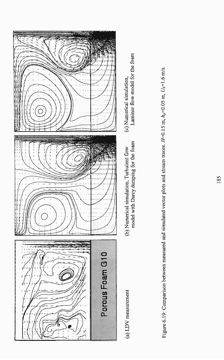
6 a a ii
f .o
ii O
6
o
c
o
6
o
•c a B
B > '^ 0 ^
^ -- ^
i=5~ i .2 ^ ta > ^ o 3 t-l .is •I* 3 o 1 6
g
1/3
0) s >
9 '5
B
:5 in
o o II
B in
o
ai ii O CO
•4—»
B CO
i3 (Zl
X) C CO
on o
• p . l - l
o - t - l
o > <U
>-» c«
3 e c
l-l
c« CO
d
ii X
o
•y
6 O U 6\
I
in (X)

VO
:^
in
o
O
^. Vi <U O CO l-l
(U
-a CO
>
S
-a c CO
l-l
CO
C ii (U
•t-t (U
c o
a, S o U o (N
IX,
VO oo

VO
^
i n
o d II
i n
o d
ii O CO
is
ii h (Zl
^3
l-l
o • 4 - " o ii >
13 ii to 3
13 C CO
'O ii ^ 3 (/3 CO ii
oo
g a
B a
X c o CO
a 6 o
U
CO
vd a l-l

0.40
0.35 -
0.30 -
^ j 0.25
0.20
0.15
0.10
• A
•
Visualisation Measurement SimulationT SimulationL
0.04 0.06 0.08 0.10
Hm 0.12 0.14 0.16
Figure 6.22: Change in the radial position ofthe centie ofthe dominant re-circulation as a fiinction ofthe fluid height for the GIO foam with hp=0.05 m. RfR is the normalised radial distance of the centie of the dominant recirculation from the centreline. H is the height of the fluid layer above the porous foam.
U . D
0.5
0.4
0.3
0.2
n 1
•
-
i
•
1
•
•
•
A
1 1 1 .
• • A •
Visualisation Measurement SimulationT SimulationL
t
• A
0.04 0.06 0.08 0.10
Hm
0.12 0.14 0.16
Figure 6.23: Change in the axial position ofthe centie of tiie dominant re-circulation as a function ofthe fluid height for the GIO foam with hp=0.05 m. He/His the normalised axial distance ofthe centre ofthe dominant recirculation measured from the interface between the fluid and the porous foam. His the height ofthe fluid layer above the porous foam.
188

•1.0
-0.2
-0.4
•0.6
•0.8
•1.0 0.0
LDV
CFDL, 200x200
CFOT, 200x200
z/H=0.067
0.2 0.4 0.6
r/R
1:1 0.0
-1.0
•1.0
-1.0
•1.0
-1.0
•1.0
-0.2
•0.4
-0.6
-0.8
-1.0
-0.2
J 4rj
J 1/ L T~
of
o/
9 1
«/ o /
r
•t , — r -
M • • • -»• ^
.
0 LDV
CFDU 200x200
z/H'O.g
2m^.7
z/H^.5
z/H=0.3
z/H'0.1
z/H=0.067
. 0.6
(a)
r/R
(b)
0.8 1.0
Figure 6.24: Axial velocity profiles in the fluid layer for /f=0.15 m, hp=0.05 m, Ub=\.6 m/s. Frames (a) and (b), respectively, represent simulations with a flat and fufly developed profile at the exit ofthe iet.
189

•1.0
•1.0
-1.0
LDV
CFDL. 200x200
CFDT, 200x200
z/H=0.B7
-1.0
-0.2
•0.4
•0.6
•o.e
0.0
z/hhO.7 I • n
8 " 1
0.2 0.4 O.e
r/R
(a)
z/hhO.5
z/H=0.3
z/H=O.U
z/H=0.09
0.8 1.0
(b)
Figure 6.25: Axial velocity profiles in the fluid layer for i/=0.1 m, hp=0.05 m, Ub=l.6 m/s. Frames (a) and (b), respectively, represent simulations with a flat and fully developed profile at the exit ofthe iet.
190

-1.0-
^ I n ,— — a , -
0 LDV
— CFDL, 200x200
CFDT, 200x200
z/H'0.9
z/H''0.7
Z/H'0.5
z/hhO.3
i/hh'0.22
z/H'0.18
0.8 1.0
-1.0
-1.0
-1.0
I •1.0
-1.0
-1.0
•0.2 -0.4
-0.6
-0.8
-1.0
•0 .2 ' 0.0
o LDV
CFDL. 200x200
CFDT, 200x200
z/H=0.9
z/H'O./
zM'O.S
Z/H'0.3
z/H=0.22
z/H'0.18
0.2 0.4 0.6 0.8
r/R
(a) (b)
Figure 6.26: Axial velocity profiles in the fluid layer for H=0.05 m, hp=0.05 m, U-6=1.6 m/s. Frames (a) and (b), respectively, represent simulations with a flat and fully developed profile at the exit ofthe jet.
191

•1.0
•1.0
3
-1.0
-1.0
0.0 •0.2
•0.4
•0.6
•0.8
•1.0
CFDL,200x200
^.''•0
V'l. 'O.S
/ ^
z/\,'0.7
zJf^-O.S
^^,-0.3
Z/,,'0.1
•
1 1 1 1
%
D.O —
•0.2
•0.4
•0.6
-0.8
• L O
CO
CFDL. 200x200
(yOT, 200x200
V,°'0
2^p=0.9
zj^g'0 7
z/1,-0.5
_ ^
z/^,-0.1
r/R
0.4 0.6 0.8
r/R
(a) (b)
Figure 6.27: Axial velocity profiles in the foam for H=0.15 m, hp=^0.05 m, Ub=l.6 m/s. Frames (a) and (b), respectively, represent simulations with a flat and fully developed profile at the exit of the jet.
192
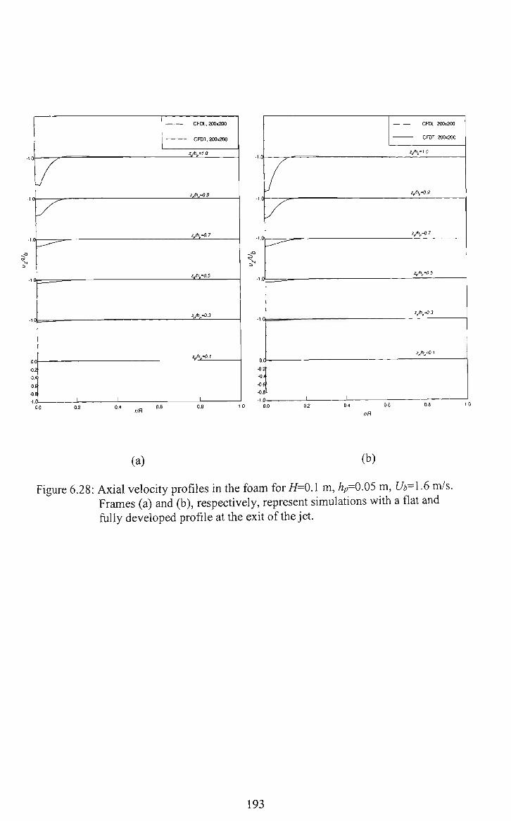
<
0,0 —
•0.2
•o" -0.6
•0,8
•I.C —
0,0 '•' r/R °'
CFDU 200x200
CFDT, 200x200
^A-'g
Zjh„-=C.9
A- "-
zJh^-O.S
^A-g-3
zJh-0.1
C
O.e-
•0.2-
•0 . ' -
•0.6
-0.8
-1.0-1.0 0.0
I
0.2
CFDL. 200x200
CFDT. 200x200
Vh,-1,0
r/R
zJh^-OS
tJh-0.7
z^^'O.S
zJt<,-0.3
z^p'^1
(a) (b)
Figure 6.28: Axial velocity profiles in the foam for//=0.1 m, hp=0.05 m, Ub=l.6 m/s. Frames (a) and (b), respectively, represent simulations with a flat and fiilly developed profile at the exit of the jet.
193

!:
o.oh <l.2
•0.4
•0,6
•0.8
r/R
CFDL, 200x200
CFDT. 200x200
^ , = ' . 0
zfy'O.g
z^,-0.7
z/1,'0.5
2/1,-0.3
zfy-O.I
-1,0.
^
0.0
•0.2
•0.4
•O.e
-o.t-
-1,0 0,0
CFDL. 200x200
CFDT. 200x200
z/,-10
zJh^'<}-9
^,-0 7
z/<,-O.S
z/1,-0.3
z/i,-0.1
(a) (b)
Figure 6.29: Axial velocity profiles in the foam for//=0.05 m, hp=0.05 m, Ub=l.6 m/s. Frames (a) and (b), respectively, represent simulations with a flat and fiilly developed profile at the exit of the jet.
194

0.2C
0.2C
0.2C
i
0.20-
0.20
o.ie
0.1S
0.08 •
0.04
0.21
0.161 0.0
o LDV
— CFDL. 200x200
CFDT, 200x200
z/H'0.9
X ^
zM=0.7
t
0.2
z/H^O.5
z/H=0.1
06
r/R
(a) (b)
Figure 6.30: Radial velocity profiles in the fluid layer for i/=0.15 m, hp=0.05 m, Ub=l.6 m/s. Frames (a) and (b), respectively, represent simulations with a flat and fiilly developed profile at the exit of the jet.
195

0.20
0.20 -- Kzr: • 7
0.20
0.20
0.16 0.0 0.2 0,4
LDV
CFDL, 200x200
CFDT, 200x200
Z/H=0.87
z/H=0.7
z/H=0.5
2/H=0.3
Z/H'0.11 u * u I
Z/H=0.09
0.20
0.20
, " J f °—^=
020
0.20
0.20
0.16
0.12
0.08
0,04
" ^
0.16 0.8 1.0 0.0
r/R
/
l/h'
o LDV
CFDL, 200x200
CFDT, 200x200
0.2 0.4 0.6
r/R
2/H=0.87
z/H=0.7
z7H^.5
z/H'O.S
z/H'0.11
z/H=0.09
0.8 1.0
(a) (b)
Figure 6.31: Radial velocity profiles in the fluid layer for H=0.1 m, ^p=0.05 m, Ub=l.6 m/s. Frames (a) and (b), respectively, represent simulations with a flat and fully developed profile at the exit ofthe jet.
196

050 -^^r:^
0.20
« 0.20
0.20
0.20
0.16
0.12
0.08
0.04
0.20
016
/
o LDV
CFDL, 200x200
CFDT, 200x200
z/H'0.9
/ V ^ 0.0
z/hhO.7
" " -
Z/H'0.5 ° " - -
0.4
Z/H'0.3
z/H'0.22
z/H'0.18
0.20
0.20
0.20
0.8 1.0
0.20
0.20
0.16
0.12
0.08
0.04
0.20
0.16
y' - . - ' ^
»1? J-^ °
•
' "-^^ "
^
V ^
•
V ^ y
»
•<^ > : v ^ \ J
/\//VV.
—.^ a_
0 o
o
.
r-^A—
0 LDV
CFDL, 200x200
Z/H'0.9
° • • ^ ° °-» . - „ . • > .
2/H=0.7
^ H = a 5
Zi'H=0.3
.
Z/H'0.22
Z/H'0.18
0.0 0.6 0.8
r/R r/R
(a) (b)
Figure 6.32: Radial velocity profiles in the fluid layer for H=0.05 m, /jp=0.05 m, Ub=l.6 m/s. Frames (a) and (b), respectively, represent simulations with a flat and fully developed profile at the exit of the jet.
197

(a) (b)
Figure 6.33: Radial velocity profiles in the foam for//=0.15 m, hp=0.05 m, Ub=l.6 m/s. Frames (a) and (b), respectively, represent simulations with a flat and fully developed profile at the exit ofthe jet.
198

CFDL. 200x200
CFDT. 200x200
z/1,'1.0
(a) (b)
Figure 6.34: Radial velocity profiles in the foam iovH^O.l m, hp=0.05 m, Ub=l.6 m/s. Frames (a) and (b), respectively, represent simulations with a flat and fully developed profile at the exit of the jet.
199

0.20
020 0.16 0.12
o.oe 0,04
0,0 0.4 0,6
r/H
CFDL, 200x200
CFDT. 200x200
ZJh,-tO
Z^P=0.9
2/1,-0.7
z/1,'0.5
z/1,-0.3
z/,-0.1
t
0.20.
0.16
0.12
0.06'
0.04
OOOL
CFDL200x200
CyDT. 200x200
z/1,'07
z/ti,-Oi
z/1,-0.3
1/1,-0.1
r/R
(a) (b)
Figure 6.35: Radial velocity profiles in the foam for i^=0.05 m, hp=0.05 m, (76=1.6 m/s. Frames (a) and (b), respectively, represent simulations with a flat and fully developed profile at the exit of the jet.
200

1 0.10—'-»=*-'
• LDV
CFDL. 200x200
CFDT, 200x200
O10
z/H=0.9
- » • » • t B
0.10 / *^>iii 1 1 n 1 T
0.10-1 ^ -^ - i—«-T --« ^ -
OlO
0.08
0.06
0.04
0.02
Q.OO 0.0
z/H=0.7
• * • - • * » " * . 1 * . - « i - .
Z/H=0.5
* * - • —.-»^->-»-.
Iz-v - _ 0.2 0.4 0.6
r/R
z/H=0.3
Z/H=0.1
Z/H=0.067
t i i • <-i
0.8 1.0
0.10
0.10
0.10
> LDV
CFDU 200x200
CFDT. 200x200
-*— . . . . • . . -
0.10-" 2»= .«=*=«=
I\_
0.10
0.08
0.06
0.04
0.02
0.00
rv
z/H=0.9
zM=0.7
- t t J
zM'0.5
z/hhO.3
z/H=0.1
zM-0.067
(a) (b)
Figure 6.36: Turbulence kinetic energy profiles in the fluid layer for H=0.15 m, hp=0.05 m, Ub=l.6 m/s. Frames (a) and (b), respectively, represent simulations with a flat and fiilly developed profile at the exit of the jet.
201

o
• L . . 0.10 1 ^ " '
010
o LDV
CFDU 200x200
CFDT, 200x200
z/H'0.B7
-0 1 a_ _fl 2 2 e o o a
L -»—s—» » 2 s a 1 " ° •> . . ~ n
OlO JL^
0 . 1 0 - i — ^ ^
O10
0.08
0.06
0.04
002
z/H'0.5
_a s It s o o o ° o
z/H'0.3
. 9 9 2 2 S fi o o ft o Q
—a ^ ^ a a Q !
z/H=0.Q9
0.10
0.10
0.10
f
0.10
- 8 • " o P . ° " - . O O P . I
0.4 0.6 0.8 1.0
r/R
0.10
0.08
0.06
0.04
0.02
0.00-0.0
LDV
CFDU 200x200
CFDT, 200x200
1 2m=Q.67
i J S fi fi 0 0 O O o O O O O O f f o
' ^ q °
Z/H=0.7
- a fi 2 2 " 0 o o q P o o e o Q
IN. z/H=0.5
" " " Q ° ° o o o
i x _ z/H'0.3
_a fi a ° o a o o o
2'H=0.ir
- f i fi fi fi B B a a a a a •
*> • . a t, o , I
0.2 0.4 0,6
r/R
0.8 1.0
(a) (b)
Figure 6.37: Turbulence kinetic energy profiles in the fluid layer for H=0.1 m, hp=0.05 m, Ub=l.6 m/s. Frames (a) and (b), respectively, represent simulations with a flat and fully developed profile at the exit of the jet.
202

0.10
O10
i
•> LDV
CFDL, 200x200
CFDT, 200x200
z/H=0.9
IB f " . . P ° o o
9
I » g n
OlO M n n n
e
10—IAU_*=
0.10
0.08
0.06
0.04
0.02
OOO
A.
0.0 0.2
z/H'0.7
-fi fi fi a , t> a
z/H'0.5
-fi 2 B a a o o n e e .
z/H=0.3
z/H=0.22
_ f i 2 a a o a o a a
ZW'O. (S
_fi - a a " • a a -a e o a o
0 . 1 0 1 ° B fi fi B a o o a 2
OlO
O LDV
CFDU 200x200
CFDT, 200x200
°A zm=0.9
_ a Q o <t a
1 " " " " tU -
0.10
f
0.10
0.10
0.08
0.06
0.04
0.02
0.00
< > ft n n
^ ' * " " " " TT
I \ n n I " i n
- f i a 8 g a a a a a a
I y n n a fi " a .
zi'H-O.S
—a a a a a a a y .
z/H=0.3
Ji a 2 S 2 - e fi a a p a n e
Z/H'0.22
- f i 2 fi a a o a a a a
2 I fi fi .fi 2 fi B '
0.4 0.6
r/R
0.8 1.Q 0.0 0.2 0,4 0.6
r/R
(a) (b)
Figure 6.38: Turbulence kinetic energy profiles in the fluid layer for//=0.05 m, hp=0.05 m, Ub=l.6 m/s. Frames (a) and (b), respectively, represent simulations with a flat and fully developed profile at the exit of the jet.
203

8 S ? ^
o
I I 2 § g S S, 8 '
HA
^
77/V
^ ? ^ S
CO
VO
l-l
•a 1
, , a T3 O 6
X -«-> ^
CO
a ii X •4—>
C • . — 1
t )
(+5 O ^ a. >> l-l ii
o (1) c
.^ C) G <U 3
-s 3 H a^ m VO (U
:::? T3 c: (3
6 »n o d II
-« ,C • .—1
B i n o d II i
^ - s O
'O c m fc: ^ o 4 —
. i j
e i n
'—' o J! : i ; ,^--«s
C3
"5 g i§ S ^ 8 ' [Ii
O CM
n/v

Chapter 7
Application: Modelling of natural convection heat and mass transfer in hygroscopic porous media 7.1 Introduction
The effect of interaction between a turbulent fluid flow overlying a porous
layer was inferred experimentally and numerically in the previous chapters. Having
secured the modelling of this interaction on a firm footing, the research was applied to
an industrially important problem. The problem involves the interaction of a
turbulently flowing fluid and a hygroscopic porous medium.
Previously published experimental and numerical investigations of natural
convection flows in a clear fluid overlying a saturated porous medium have been
confined to studies in which the flow in the clear fluid is in the laminar regime. In
many practical situations, however, one encounters systems in which the heat and
mass transfer is significantly affected by turbulence, at least in the fluid region. Such
a two-layer system can be encountered in the storage of porous materials such as
grains, fhiits and catalysts. Thermal insulation in buildings and geothermal reservoirs
are also modelled as a two-layer system. In these examples, the fluid (which is
generally air), can often be turbulent. It is well established from natural convection
studies in clear fluids (the experimental studies of Cheesewright et al, 1986a;
Kirkpatiick and Bohn, 1986 and numerical studies of Henkes, 1990 and Kenjeres and
Hanjalic, 1995), that the enclosure dimensions contribute to whether the flow is
laminar or turbulent, hi enclosures the size of typical rooms, the flow of air is
normally turbulent due to the large Rayleigh numbers encountered. Thus, one cannot
ignore turbulence as a factor which enhances heat transfer, and hence moisture
migration in such two layer systems if there is a significantly large fluid layer. In the
porous medium, turbulence will not persist if the medium is of a sufficientiy low
permeability. Thus, one could assume a laminar regime in die porous medium. Flow
visualisations presented in chapter four and the corresponding simulations presented
in chapter five have revealed that for low permeability porous media with
205

A < O(l0 *), the fluid layer and the porous medium could be regarded to be operating
in the turbulent and laminar regimes respectively.
In the literature, there is a limited number of studies on systems that contain a
fluid overlying a porous medium. Numerical and experimental studies of such
systems have been concemed with two particular physical configurations. The
heating from below case, which is analogous to the Rayleigh-Benard problem, has
been stiidied by Poulikakos et al (1986), Poulikakos (1986), Chen and Chen (1989)
and Chen and Chen (1992) among others. The heating from the side problem has
been studied by Beckermann et al (1988), Song and Viskanta (1994) and Singh et al.
(1993). All of these studies have been carried out for the laminar flow regime.
The present work is a continuation of the study carried out by Nguyen (1987)
who presented a method of solving the equations of heat, mass and momentum
transport in bulks of stored grains that have peaked geometries. In that paper the
effect of turbulence in an overlying fluid layer was not considered probably due to the
large computational times required to solve transient problems in natural convection
with turbulence. However, with the ready availability of faster computers, such
simulations with more realistic physical conditions can be carried out within
reasonable times.
A general method of analysing systems witii a fluid overlying a hygroscopic
porous medium where tiirbulence in the fluid layer is important is presented in this
chapter. A hygroscopic porous medium has been chosen for the present model to be
useful in modelling stored agricultural produce such as grains that are hygroscopic in
natiire. In such systems the commodities in warm regions tend to become dry, and
convection currents carry moisture to cooler regions which become moist.
Components of the model have been validated with previous experimental and
numerical results, which were found to be similar to the present system. An
application of moisture migration through a representative hygroscopic porous
medium is presented to emphasise the potential application of die model. A two
dimensional system has been used so that the salient featiires of the work are
explicated with clarity.
206

7.2 Governing equations
The goveming equations for fluid flow and heat tiansfer for tiie case stiidy can
be represented as:
Equation of continuity:
du dv ^ — -I-— = 0 dx dy
(7.1)
Momentum equation in the x-direction:
du p.u du p„v du dp d Pa— + — + -^ = —— + —
dt (j) dx ^ dy dx dx ip + P>i2
du
dx
+ • dy
( -^ du dv (^pu Cp(/>uQ
K Pa T^xn
(7.2)
Momenmm equation in the_y-direction:
dv pu dv pv dv dp d
dt (f) dx (/> dy dy dy
d_
dx
<t>pv
(y" + /^J2 dv_
dy
- f • / M du dv^
^PagP(T-T,)
K Pa
Cp^Q
K 1/2
(7.3)
where, (f) represents porosity ofthe porous medium, K is its permeability and CF is the
Forchheimer coefficient. Pa is the density of air and Q = V w + v . The variables
have the same meaning as in Section 2.4.1.1 of chapter two. The difference in the
above momentum equations and Equations (5.4) and (5.5) is the presence of the
buoyancy term in Equation (7.3).
The eddy viscosity is represented as:
P, = PaC, (7.4)
in which c^ = 0.09.
207

It is assumed that turbulence persists only in the fluid layer, and it is rapidly
attenuated in the porous medium due to its low permeability. Thus, the eddy
viscosity, pt, applies only for the fluid layer. For the porous medium, its value is
taken to be zero.
Thus the modelling ofthe two-layer system for the application is equivalent to
the use of a laminar flow model for the porous foam in the numerical simulations
presented in the fifth chapter. As seen in chapter five, the Darcy and Forchheimer
terms vanish in the fluid layer as the fluid has infinite permeability. The porosity of
the fluid layer is taken to be unity, and a step change in porosity and permeability is
assumed at the interface between the fluid layer and porous medium.
Thermal energy equation:
Due to the presence of the hygroscopic porous medium, the thermal energy
balance assumes different forms for the fluid layer and the porous medium. The
partial differential equations for heat, mass and momentum transfer in stored
agricultural produce have been derived in Thorpe et al (1992). For the present
problem one can write.
V), eff dT dT dT + PaU + Pa^
dt dx dy
d_
dx Pr GT
dT
dx
d + —
dy Pr Gj
dT
dy (7.5)
-f PbK dW c,. dt
where, (pcK = (l - (/>)p^c^ + ^p^c^ + Wc^ + dH^
dT (7.6)
and ar = 0.9
Ca represents the specific heat of air; c^ is the specific heat of liquid water. Cs is the
specific heat ofthe porous solid and A is its density. Cb is the bulk specific heat, hs is
the latent heat of sorption and pb is the bulk density. W is the moistiire content of the
porous medium on a fractional dry basis and Pr is the Prandti number of air.
The term Wc^ arises due to the presence of moistiire in tiie porous medium.
The term H^ represents the integral heat of wetting, tiie details of which can be found
208

in Sutheriand et al (1971). The last term on the right hand side represents die heat of
sorption. It should be noted that for the fluid layer, the integral heat of wetting, H^,
and the heat of sorption, hs, would vanish since these are terms only associated with
die porous medium. Again, for the porous medium the eddy viscosity term is zero, as
turbulence is absent in the porous medium
Turbulence kinetic energy equation:
dk_ dk_ 3^__5_ " dt " dx " dy dx
^ pAdk a
+P,+G,-p^e
dx +-dy /" + P, ^dk
a k J dy (7.7)
where, ak^l.O
Equation for the rate of energy dissipation:
de de Bf' _ 9
" dt " dx " dy dx P + Pt de
eJ dx + dy P +
pAd£ ^dy (7.8)
+(^M^k+c,,G,)-p^c^J,e)^
where, o-e=l.3, A:= von Karman's constant = 0.41, C£/= 1.44 and 0^2=1.92.
For the coefficient Ces, the form suggested by Henkes (1990) is used (see Section
2.4.1.1 in the second chapter)
Thus c 3 = tanhv/w
Note that Equations (7.7) and (7.8) apply only to the fluid layer since turbulence is
assumed to be absent in the porous medium.
Goveming equations for moisture migration in porous media
In the following description, the term porous medium implies a bulk of solid
particles, which is saturated with air. This bulk is considered to be a continuum
according to the principles of volume averaging independentiy derived by Whitaker
(1967) and Slattery (1967) discussed in Section 2.2.3 of chapter two. The term
porous solid refers to an individual particle such as grain or silica gel crystal that has
micropores within which moisture can be adsorbed.
hi case of stored agricultural or horticultural produce and hygroscopic porous
media such as silica gel (used as a desiccant), the total moisture content is the sum of
209

the moisture content of the air and the solid, which is porous. Since the porous solid
and the surrounding air carry moisture in them, the total moisture balance involves the
concentiation of moisture in air as well as in the porous solid. Thus one needs to take
into account two moisture balances namely the intra-granular and inter-granular
moisture balances.
Intra-granular moisture balance dW dt
= DjW^-W) (7.9)
where W is the moisture content of the porous medium on a dry basis. We is the
equilibrium moisture content of the porous medium and Das is a rate coefficient for
moisture exchange between air and porous medium.
In the present study, it is assumed that the solid is always in thermodynamic
equilibrium with the surrounding air. This assumption is correct when the rate of
intia-granular moisture migration is much faster than inter-granular moisture
migration. In case of small particles like grains or silica gel crystals, this will be tme
at the low air flow rates encountered in natural convection (Thorpe and Whitaker,
1992). However, one needs to incorporate the above equation in tiie solution
procedure for large particles such as fiiiits.
Inter-granular moisture balance
The equation that govems the concentiation of moisture in the air has a
slightly different form in tiie fluid and porous layers due to the contribution of the
solids to the air moisture balance in the porous medium. The moisture balance for the
porous medium can be represented by:
, dw dw dw dW d f ,, ?hAl\ p dw Sc dx
d
dy
p dw Sc dy
(7.10)
where w is die air moistiire content on a dry basis and Sc is the Schmidt number of air.
The moisture balance in the fluid layer can be written as;
210

, dw dw dw d (hp — -I- p u — + p„v— = p„ —
dt dx dy dx
P ^Pt
LV Sc (7^
dw
dx
d
dy LV
Sc o"„.
dw
dy (7.11)
where, o-;„ = 0.65.
The eddy viscosity, pt, has been invoked only in the equation for the fluid layer.
An order of magnitude analysis is now carried out on Equation (7.10) to
determine the relative significance of each term for low permeability porous media
such as grains. Significant variations in the moisture content occur only over a long
period of time, which is on the order of months. When expressed in seconds, a time
scale of t = O\l0^) seconds is obtained. During such a time period, there is a
variation in the moisture content on the order of Aw = 0(10"^) and AW = 0(10"') on
a kg of moisture/kg dry basis.
Typical velocities encountered in natural convection flows in porous media of
low permeability (/)« = o(lO"*)), is w = o(lO"^) m/s for relatively high Rayleigh
numbers [Ra = o(lO'°)). This value has been verified by carrying out computations
for these Darcy and Rayleigh numbers without moistiire migration. It is assumed that
moisture migration will not significantly alter the velocities. The length scale for such
Rayleigh numbers is l = Ax = 0(1) m. The density of air, p^ = 0(1) kg/m^ and the
bulk density ofthe porous medium, p^ = 0(10^) kg/m^ are used.
Thus one can write
dw "¥ = r 10-2 A 1-
10' = o(io-')
/
dw pu— = 0 ^" dx
f IxlO"
10 -2 \
dW _
o(io-^) (7.12)
10 2 10 -1 ^
10' = o(io-^)
The analysis shows that the advection term is balanced by the change in tiie
solids moisture content and tiiat tiie rate of change in the air moisture content is
211

negligible in comparison. The molecular diffusion term may be significant close to
the walls because the velocity component normal to a wall is small, but steep
concentration gradient in this direction could exist. Thus, molecular diffusion cannot
be neglected. The result enables one to neglect the first term on the left-hand side of
Equation (7.10) thus allowing the computation of fF explicitiy in the porous medium.
One problem encountered in a previous study by Chen et al. (1999) was with the
transient computation of such systems. These authors had used an implicit solution
procedure by including all terms in Equation (7.10). This problem is overcome in the
present study by using the above explicit procedure. The present formulation also
allows one to take large time steps to study moisture migration once the temperature
and velocity fields have evolved almost to a steady state, because the moisture field
does not significantly affect the temperature and velocity fields. The ability to take
large time steps during the process of computations is important due to the large time
scales (days or months) encountered in such systems.
The present calculations start with an initial value for moisture content of the
porous medium. This value is used to calculate the moisture content of air in the
porous medium using an appropriate sorption isotherm. The moisture content of air in
the fluid layer is calculated by using Equation (7.11).
Silica gel is used as the representative hygroscopic porous medium for the
study because its properties are quite well established and it can adsorb up to 50% of
its dry mass of water, hence any effects due to its hygroscopy will be quite
pronounced.
The sorption isotherm ofthe gel is represented by
W = 0.5r (7-13)
where, r = - ^ represents relative humidity of air. The saturation pressure, psai, is Psa>
given by Hunter's (1987) expression:
6x10" ^ 6800^ —1—exp T abs
(7.14)
212

The moisture content ofthe interstitial air in the porous medium is calculated by using
the relationship,
0.622;? w- 0.622P,,„-p
where Patm is the atmospheric pressure.
(7.15)
7.3 Problem definition, boundary and initial conditions
As a case study for the proposed model, moisture migration in a rectangular
cavity of aspect ratio 2 with half the cavity filled with silica gel is chosen. A Rayleigh
number, Ra = 10'° and a Darcy number. Da =10' are chosen for the study. These
numbers translate to a total system height, H, of about 2 metres with a width, D, of
about 1 metre. The Darcy number chosen is typical for a storage system that contains
particles such as wheat with a diameter of about 3 mm. Figure 7.1 shows a schematic
diagram ofthe simple two-dimensional geometry considered for the case study.
< D •
y
Fluid layer
H
Figure 7.1: Schematic diagram ofthe system used for the case stiidy.
213

Typical boundary and initial conditions of a storage vessel are considered for
the case stiidy. These can be summarised as follows for the mean quantities:
u = v = 0 at X = 0, Dandy = 0,H
r = 7;=10°C atJc = 0,Z)and>^ = / /
at>; = 0 ^ = 0 dy
Tporous=T, =30'C att = 0 (7.16)
r„,. = (T,^T,^
V
= 0 dW _dw
dx dx dW 5>v_
at? = 0
at X = 0, £) and >; = 0, / /
atx = 0,D andy = 0,H dy dy
where Tpowus and Tair are the initial temperatures of the porous medium and air,
respectively.
As seen from Equation (7.16), zero gradient boundary conditions are applied
to the moisture content, w, of the air and moisture content of the porous medium, W.
This over specifies the system as, strictly, the gradient of the moisture content of air
should be zero at the impermeable boundaries, and the moisture content of the solids
is a dependent variable. However, specifying the gradients of the moisture contents
of both air and the solids results in a computationally stable and accurate solution.
The mean variables are solved right up to the wall without using any wall
functions. However, for the turbulent variables, k and e, wall functions obtained from
the inertial law are applied at the first inner grid point (see Section 2.4.1.1.1 in chapter
two):
.^,eM KX
where v is the friction velocity defined by v* wall
where T^^ is the wall shear stiess calculated from z^n = p
and X is the normal distance from the wall.
^dv'
\dx j^„
(7.17)
214

As mentioned before in Section 3.2.2 of chapter three, the above modification
to the standard k-e model has been suggested for natural convection flows, because
the wall fiinctions that normally apply for forced convection flows are not applicable
for natural convection flows.
The volume-averaged velocities are continuous across the interface since tiiey
are continuous across the fluid-solid and fluid-fluid segments of the interface. The
temperature, heat flux, moisture content of air and porous medium and the gradient of
the air moisture content are continuous at the interface due to die same reason. Due to
the use of the Brinkman extended Darcy flow model for the porous medium, the
gradients of the velocities or the normal and tangential stresses also become
continuous across the interface.
For the turbulent variables, k and e, at the interface of the fluid and low
permeability porous layer turbulence is assumed to be completely damped as implied
by the flow visualisation experiments in chapter four. For this reason the conditions
at the interface of the fluid and porous layer, for k and e, are taken to be identical to
the conditions at an impermeable wall.
7.4 Validation of the model
For the present problem, two configurations were used to validate components
ofthe model. The simulations and experimental work of Song and Viskanta (1994)
were used to validate the Brinkman Forchheimer extended Darcy flow model for a
system consisting of a fluid layer adjacent to a porous layer. The schematic diagram
in Figure 7.2(a) represents the square cavity adopted by Song and Viskanta (1994)
witii adiabatic top and bottom walls and differentially heated side-walls. The
tiirbulence model was validated with the experimental results of mixed cavity natural
convection reported by Kirkpatrick and Bohn (1986) for their HCCC (Hot-Cold-Cold-
Cold) configuration because the boundary conditions used closely resembled die
present boundary conditions. Figure 7.2(b) represents a schematic diagram of the
HCCC configuration of Kirkpatiick and Bohn (1986) with a square cavity having a
hot bottom wall and cold top and side-walls.
215

Q=0
Th
Q=0 (a) Song and Viskanta (1994)
Th
(b) Kirkpatiick and Bohn (1986)
Figure 7.2: Schematic diagram ofthe configurations used for validation ofthe model.
7.4.1 Method of solution
As discussed in Section 2.5 of chapter two, the model equations are discretised
using the control volume formulation and are solved using the SIMPLE algorithm.
The upwind/central hybrid scheme is used for discretising the convection terms. The
diffiision terms are discretised using the second order cential scheme. Non-uniform
grid spacing generated by the sine fiinction given in Equations (3.10) and (3.11) was
used to account for the large gradients in velocity and temperature wherever
applicable. The simulation is assumed to have reached a converged solution when the
sum of the normalised absolute mass, momentum and thermal energy sources for all
contiol volumes have individually reached a tolerance of 1x10" (see Equation (2.72)
for an example). The sources were normalised by dividing them by the total number
of contiol volumes.
7.4.2 Results and discussion for model validation
For the prediction of tiie Song and Viskanta (1994) experiments, an 80x80
grid was found to be sufficiently accurate after carrying out a grid refinement study.
Grid points were closely spaced near the walls and at the interface between the fluid
216

and porous layers to accommodate the steep gradients in these regions. The unsteady
terms in the momentum and thermal energy equations were neglected, and a steady
formulation was used. Figure 7.3 shows the comparison between die present
simulations and experimental and simulated results of Song and Viskanta (1994) for
their experiment 3.
(a) Isotherms (b) Stieamlines
Simulations of Song and Viskanta (1994). Reproduced from their Figures 4(b) and (c).
c) Isotherms d) Stieamlines
Present simulations
217

• • • • •
y/H = 0.9 y/H = 0.52 y/H = 0.48 y/H = 0.1 y/H = 0.1, Exp, y/H = 0.5,Exp, y/H = 0.9, Exp,
x/H
(e) Comparison with experimental temperature profile of Song and Viskanta (1994). Experimental points have been reproduced from Song and Viskanta (1994), Figure 4(d).
Figure 7.3: Comparison ofthe present simulation with experiment 3 of Song and Viskanta (1994).
The streamlines and isotherms obtained in the present predictions are in good
agreement with their predictions as seen from Figures 3(a) to 3(d). The predicted
temperature profiles are also similar to the measured results of Song and Viskanta
(1994) as seen from Figure 7.3(e). The major discrepancy between the measured and
predicted temperature profiles is found at y/H=0.l in Figure 7.3(e). Song and
Viskanta (1994) attributed this discrepancy to the continuum model used. Steeper
changes in velocity and temperature are encountered in the lower portions of the
cavity (streamlines and isotherms are more closely spaced in the lower portions of the
cavity on the fluid side) as one goes from the fluid layer to the porous layer. It is
conjectured that the continuum model does not correctiy predict these steep changes.
However, the general agreement between the modelled and experimental profiles is
adequate, as pointed out by Song and Viskanta (1994). Moreover, in the case of die
present system one would not have such steep gradients as one goes from the fluid
layer to the porous medium. Hence, an even better prediction ofthe system in Figure
7.1 is expected with the present model.
218

For the simulations of the experiments of Kirkpatrick and Bohn (1986),
60x60, 120x120 and 240x240 non-uniform grids were used in order to study the effect
of grid refinement. For these simulations, a Rayleigh number of 10'° was used with
the working fluid as water. All the physical properties were taken at the bulk fluid
temperatiire. Table 7.1 gives a comparison ofthe Nusselt numbers at the four walls
for the three grids considered. For all computations the difference between the hot
wall and cold wall Nusselt numbers was less than 4% when die convergence criteria
were met. Also, the difference between the Nusselt numbers ofthe vertical walls was
less than 1%. It can be seen that with a change in the grid size, the maximum
variation in the Nusselt number occurs at the vertical walls, hi going from a 120x120
to 240x240 grid, the top and bottom wall Nusselt numbers vary by less than 1%.
However, the vertical wall Nusselt numbers vary by almost 10%. Therefore, the
solution is still not grid independent for the finest grid used. Finer grids were not
used for these simulations as they lead to large computational times. F6r example, the
simulation time required for the 60x60 grid was approximately 30 minutes in a
Pentium 11 350 MHz machine. In refining the grid from 60x60 to 120x120 the
computational effort increases by a factor of about four. This means that even for the
240x240 grid approximately 8 hours is required to complete one mn.
Table 7.1: Grid refinement study for the simulations ofthe experiments of Kirkpatrick and Bohn (1986) using wall Nusselt numbers.
Grid
60x60 120x120 240x240
Left Wall 64.77 75.82 83.82
Right wall
64.34 75.54 83.61
Top Wall 110.1 109.4 109.2
Bottom wall
238.9 251.4 252.4
Kirkpatrick and Bohn (1986) used the average of the four hot/cold wall
temperatiires as the bulk temperatiire. The wall to bulk temperatiire difference was
used to evaluate die Nusselt numbers. For the HCCC configuration, they found that
the Nusselt number to Rayleigh number relationship collapsed to a single correlation
for all four walls, namely:
Nu = 0.3A6Ra'''' (7.18)
The coefficient in this definition of the Nusselt number is calculated for all
four walls. These results are given in Table 7.2. The maximum error in the
219
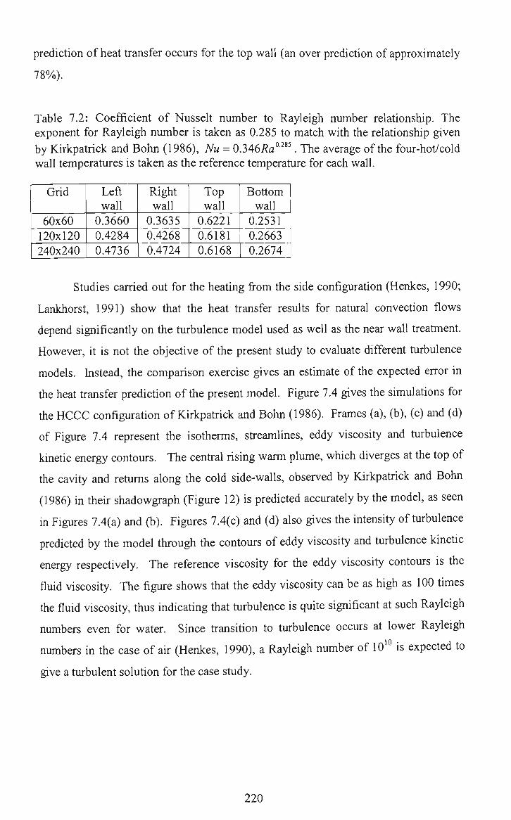
prediction of heat transfer occurs for the top wall (an over prediction of approximately
78%).
Table 7.2: Coefficient of Nusselt number to Rayleigh number relationship. The exponent for Rayleigh number is taken as 0.285 to match with the relationship given by Kirkpatrick and Bohn (1986), Nu = 0.3A6Ra°^'^^. The average ofthe four-hot/cold wall temperatures is taken as the reference temperature for each wall.
Grid
60x60 120x120 240x240
Left wall
0.3660 0.4284 0.4736
Right wall
0.3635 0.4268 0.4724
Top wall
0.6221 0.6181 0.6168
Bottom wall
0.2531 0.2663 0.2674
Studies carried out for the heating from the side configuration (Henkes, 1990;
Lankhorst, 1991) show that the heat transfer results for natural convection flows
depend significantiy on the turbulence model used as well as the near wall treatment.
However, it is not the objective of the present stiidy to evaluate different turbulence
models. Instead, the comparison exercise gives an estimate of the expected error in
the heat tiansfer prediction of tiie present model. Figure 7.4 gives the simulations for
the HCCC configuration of Kirkpatiick and Bohn (1986). Frames (a), (b), (c) and (d)
of Figure 7.4 represent the isotherms, stieamlines, eddy viscosity and turbulence
kinetic energy contours. The cential rising warm plume, which diverges at the top of
the cavity and retiims along the cold side-walls, observed by Kirkpatrick and Bohn
(1986) in tiieir shadowgraph (Figure 12) is predicted accurately by the model, as seen
in Figures 7.4(a) and (b). Figures 7.4(c) and (d) also gives the intensity of tiirbulence
predicted by the model through die contours of eddy viscosity and tiirbulence kinetic
energy respectively. The reference viscosity for the eddy viscosity contours is the
fluid viscosity. The figure shows that the eddy viscosity can be as high as 100 times
the fluid viscosity, thus indicating that tiirbulence is quite significant at such Rayleigh
numbers even for water. Since tiansition to tiirbulence occurs at lower Rayleigh
numbers in the case of air (Henkes, 1990), a Rayleigh number of 10'° is expected to
give a turbulent solution for the case study.
220

15 14 13 12 11 10 9 8 7 6 5 4 3 2 1
e 0.875 0.813 0.750 0.688 0.625 0.500 0.319 0.304 0.295 0.290 0.284 0.250 0.188 0.125 0.063
(a) Isotherms
(b) Stieamlines
Figure 7.4 (For caption, see next page)
15 14 13 12 11 10 9 8 7 6 5 4 3 2 1
V
0.018 0.017 0.016 0.015 0.013 0.012 0.011 0.010 0.009 0.007 0.006 0.005 0.004 0.002 0.001
221

(c) Eddy viscosity contours
15 14 13 12 11 10 9 8 7 6 5 4 3 2 1
0.0043 0.0040 0.0036 0.0034 0.0032 0.0029 0.0026 0.0023 0.0020 0.0017 0.0014 0.0012 0.0009 0.0006 0.0003
(d) Turbulence kinetic energy contours
Figure 7.4: Simulation for the experiment of Kirkpatiick and Bohn (1986), HCCC configuration. i?a=10'° with the working fluid as water.
222

7.5 Case study
The geometry for the case stiidy is shown in Figure 7.1 above. A 60x60 non
uniform grid was used for the case stiidy since it was found that with a 120x120 grid,
the same simulation takes approximately four times longer with no significant change
in the accuracy of the solutions. For the unsteady calculations, a time step of 0.1 s
was used until the temperature and velocity fields were almost converged in the fluid
layer. The convergence was monitored through changes in the wall Nusselt numbers.
Approximately 3000 time steps were required. The time step was then increased to
10 s, for monitoring changes in the moisture content and changes in temperature in
the porous layer. Any further increase in the time step led to divergence. Due to the
small number of space iterations between two time iterations (typically, no more than
three to four), computations for significantly large real times can be carried out in
relatively short machine times. For the largest real time calculated in the present case
study, 50 hours, a CPU time of around 5 hours was required on a Pentium II 350 MHz
machine. However, increasing the time step is desirable, as this would lead to shorter
computational times. Figure 7.5 indicates the streamlines and isotherms after the
initial 3000 iterations.
15
14
13
12 11 10 9 8 7 6 5 4 3 2 1
V
0.007 0.007 0.006 0.006 0.005 0.005 0.004 0.004 0.003 0.003 0.002 0.002 0.001 0.001 0.000
Figure 7.5: Stieamlines and isotherms for the case study after the first 3000 time steps, equal to 300 s.
223

As expected, these do not change significantly for large times in the fluid
layer. The eddy viscosity and turbulence kinetic energy profiles in the fluid layer are
similar to the profiles obtained for the experiment of Kirkpatrick and Bohn (1986), as
presented in Figure 7.4. The changes in the isotherms, moisture content of air and
moisture content of the porous medium are shown in Figures 7.6, 7.7 and 7.8,
respectively, after 10, 20, 30 and 50 hours. The heat and moisture from the porous
medium is driven towards the fluid layer through the central rising plume as seen in
Figures 7.6 and 7.7. This plume is expected to enhance the transport of heat and
hence moisture from the porous medium. Thus, the choice of a turbulence model is
important for the accurate prediction of heat transfer. Due to the heat transfer, the
core of the porous medium becomes progressively cooler, as seen in Figure 7.6.
Similarly, from Figure 7.7, one can see that the moisture content of the air in the
porous medium decreases as time progresses. Figure 7.8 shows changes in the
moisture content ofthe porous medium with time. As the air gets cooler, its ability to
hold moisture decreases, and this extra moisture is absorbed by the hygroscopic
porous medium. In case of grains, this phenomenon has important implications as it
leads to the growth of moulds in these regions, which can eventually destroy the
grains. It is clear from Figure 7.8 that close to the side-walls and in the region close
to the central rising plume in the porous medium, the moisture content of silica gel
increases. This increase becomes significant as time progresses. It is evident from
Figure 7.6 that these are regions of relative coolness in the porous medium.
It is emphasised here that the present model does not take into account
tiirbulence within the porous medium due to die low permeability of the porous
medium considered for the simulations. However, this would not be the case for
porous media of high permeability and turbulence within the porous medium will be
an important factor to be considered. As seen in chapter five, one method of doing
this would be by solving the turbulence tiansport equations in the porous medium and
accounting for the attenuation of turbulence by incorporating damping terms in the
turbulence tiansport equations for the porous medium.
224

CP C J ^ C T > O C ) C o r ^ r - ; ( X > C D L / 5 U 5 T ^ . < i - C O r O C N C N - . — •.— O
d c 3 d o c 5 d o d o o o c > c > d o d c 5 d o o
. - o c 3 5 c o r ^ U 5 L n ' < i - n c S ' - o CSICN-— •.— •.— "— ' - • . ^ • . — -.— • ^ . — C 3 5 < r ) [ ^ C D L O ' ^ r O C M
3 o O i n
O X o CO
3 o X o (N
; - i
o
ii (Zl CO
o (U
X
ii
B
^ &0
ii
o c«
c CO
U V O
u l-l
E
m Csl

^q8888888888S8888888§§ o o o o o o o o o d d d d d d d d d d d d r ; O C T > o o r ^ i x ) L O T f f r , < s i _ Q
O5fl0I^CDLr>.^C0CN^
c
.7—roi
SB^m"
o o m
CO
O .ill O c<-)
C/3
o X o (N
c« u
O
>% T3
D tzi CO O
ii X
ii B
• l-H
X +-»
• f - H
CO ^ 4 - 1
o G <u
^—» C O o 0) ;-! B i/i 'o S
_c 0)
u X
u r~ a t - l
§)
VO CM

. 8S8g8S8S8g8g8S8S8g8g8 •^ c ^ < N c s c N c s c ^ j C N C S ! c s c N C ^ l ' - • - • ^ ^ • ^ U ) i : l i : i i : l i :
• ^ O C P a o r ^ ^ C D L D M - f O C N - ^ O C7)<»rvCOLO.<) -<T)<N —
l r~^^U6 U-
l-l
O X! O i n
in • ^ 9 0 2 ' 0 :
0.2=
-7 -A .cnz-n:
00 l-l 3 O
o en
• l^ 'O-
LD
=0.2i
c« V.I 3 O
.Cl o
: cn7 '
ii CO CO
o 0)
xi
B • •-< ^ 3 ii
B CO
O l-l
O o. (U
•B CM O c B c o o D i-i 3
Csl
00
:n:2=u.2i=
c n n 7 T i ;
-0.2-
T-n::
CO l-l
3 O 43 O
ii X +-" c . .—1
<L> 00
X
u 00
r-u l-l
^ tin

7.6 Conclusions
A general procedure of simulating systems with a turbulent fluid layer
overlying a saturated hygroscopic porous medium has been presented. Emphasis has
been placed on using this model for simulating moisture migration in stored
agricultural produce. It is believed that such a model is capable of predicting tiie
moisture migration process more accurately as it accounts for tiirbulence in the fluid
layer. The level of sophistication of the turbulence model is however limited by the
comparatively large mn times encountered to simulate such systems. The model
needs to be validated further with realistic experimental data. The present model is
capable of simulating flow only when turbulence in the porous medium can be
considered to be negligible. However, this would not be the case for porous media of
high permeability. This limitation can be overcome by incorporating a turbulence
model for the porous medium with appropriate damping terms, as in the simulations
presented in the fifth chapter, for the attenuation of turbulence in the porous medium.

7.6 Conclusions
A general procedure of simulating systems with a turbulent fluid layer overlying a
saturated hygroscopic porous medium has been presented. Emphasis has been placed
on using this model for simulating moisture migration in stored agricultural produce.
It is believed that such a model is capable of predicting the moisture migration
process more accurately as it accounts for turbulence in the fluid layer. The level of
sophistication of the turbulence model is however limited by the comparatively large
mn times encountered to simulate such systems. The model needs to be validated
further with realistic experimental data. The present model is capable of simulating
flow only when turbulence in the porous medium can be considered to be negligible.
However, this would not be the case for porous media of high permeability. This
limitation can be overcome by incorporating a turbulence model for the porous
medium with appropriate damping terms, as in the simulations presented in the fifth
chapter, for the attenuation of turbulence in the porous medium.
228

Chapter 8
Conclusions and final remarks 8.1 Conclusions
The following conclusions can be drawn after having investigated the
interaction between tiirbulent flow and satiirated porous foams using numerical and
experimental methods.
1) Flow visualisation experiments revealed that the permeability of die porous foam
and the height of the fluid layer above the porous foam significantly affect the
flow pattem, at least in the fluid layer. The thickness of the porous foam affects
the flow pattem to a smaller extent. For low permeability porous foams
( A : < 10"^) it was found that there is littie change in the flow pattem in the fluid
layer from the cases without porous foams. This result led to the concept of
treating the interface between the fluid layer and porous medium as a wall in
numerical simulations for turbulent quantities such as the turbulence kinetic
energy, k, and its rate of dissipation, e. In such cases, the fluid layer and the
porous medium could be regarded to be operating in the turbulent and laminar
regimes, respectively. In case ofthe highest permeability GIO foam investigated,
{K = 2.843X10"^), the flow pattem changed significantly in the fluid layer with a
change from a single cell to a two-cell pattem. This change was observed for all
three fluid heights investigated, indicating the stiong interaction between the flow
in the fluid layer and the adjacent porous medium.
2) Three different models were used to represent the flow in the porous foam namely
a laminar flow model and two turbulence models for CFD simulations
corresponding to the flow visualisations. The aim was to infer tiie effect of the
presence or absence of macroscopic turbulence in the porous medium by stud>ing
the changes in the flow pattem, mean velocities and turbulence kinetic energy in
the fluid layer. One of the turbulence models witii only Darcy damping in the k
and e equations was found to be qualitatively superior in predicting the gross flow
pattems, especially the effect of permeability of tiie porous foam and clear fluid
229

layer height. The second turbulence model with Darcy and Forchheimer
modifications included in the k and e equations for the porous foam was found to
be qualitatively similar to the laminar flow model in its predictive capabilities.
The similarity in predictions was found to be due to the almost complete damping
of turbulence at the interface between the porous foam and clear fluid due to the
Darcy and Forchheimer modification terms thus making the flow in the porous
foam effectively laminar in nature. None of tiie three models used to represent
flow in the porous foam could adequately predict the effect of changes in the
thickness ofthe porous layer.
3) In order to further consolidate on the flow visualisations, LDV measurements
were carried out for a quantitative comparison between the CFD simulations and
the measurements. The vector plots obtained from the measurements confirmed
the development of the two-cell pattem in the fluid layer for the highest
permeability GIO foam that was investigated initially with the flow visualisation
experiments. It was found that quantitatively, the simulations predict the mean
axial velocity profiles better with the turbulent flow model with only Darcy
damping for the porous foam. For the radial velocity profiles, predictions with the
laminar flow model and turbulence model with Darcy and Forchheimer
modification terms were found to be better at the highest fluid height in a region
close to the interface between the fluid layer and porous foam. The turbulent flow
model with Darcy damping showed better agreement with the measurements for
the radial velocity as the fluid height decreased. The tiirbulence kinetic energy
profiles in the fluid layer showed relatively good agreement with predictions by
laminar and turbulent flow models for the foam.
4) Having secured the modelling of the interaction between a turbulent fluid flow
overiying a saturated porous layer on a firmer footing, the research was applied to
an industrially important case study concerning moisture migration in respiring
agricultural produce. In this case study a general procedure of simulating systems
with a turbulent fluid layer overlying a saturated hygroscopic porous medium was
developed. It is believed that such a model is capable of predicting tiie moisture
migration process more accurately as it accounts for turbulence in the fluid layer.
230

The level of sophistication of the tiirbulence model is however limited by the
comparatively large mn times encountered to simulate such systems.
8.2 Final remarks
1) As stated at the beginning of this thesis, the present research was aimed primarily
at inferring the effect of turbulence modelling in the porous medium by studying
the interaction between a turbulent fluid flow overiying a saturated porous
medium. The reason for such an indirect evaluation is due to the inability of using
measurements made at point locations in the porous medium for comparison with
simulations using volume averaged equations. A more direct approach could have
been adopted if there was a method of volume averaging the experimental results
obtained by carrying out measurements within the porous medium.
2) The present thesis can be considered to be a first attempt at inferring turbulence in
porous media and its interaction between an adjacent turbulent fluid layer using a
combination of conventional modelling and experimental techniques. However,
the use of conventional turbulence modelling stiategies such as in the present
research that is analogous to modelling turbulent flow for fluid flow in the
absence of porous media might be impracticable for many real porous media. The
use of grid based eulerian techniques such as finite volume, finite difference or
finite element methods lead to inherent difficulties in modelling flow in real
porous media. Instead, grid less lagrangian techniques such as Smoothed Particle
Hydrodynamics (SPH) could be used to study the effect of microscopic flow in
porous media on macroscopic turbulence.
231
References
Aerometrics Hardware and Software Manual, 1997, TSI Inc., Minnesota, USA.
Antohe, B. V. and Lage J. L., "A general two-equation macroscopic turbulence model for incompressible flow in porous media". International Journal of Heat and Mass Transfer, 1997, 40, 3013-3024.
Baughn, J. W. and Shimizu, S.," Heat Transfer measurements from a surface with uniform heat flux and an Impinging jet", ASME Journal of Heat Transfer, 1989, 111, 1096-1098.
Bear, J., "Dynamics of fluids in porous media", American Elsevier, New York, 1972,pp.l25-128.
Beavers, G. S. and Joseph D. D., "Boundary conditions at a naturally permeable ^^2X1'% Journal of Fluid Mechanics, 1967,30, 197-207.
Beckermann, C , Ramdhyani, S. and Viskanta R., 'TMatiiral convection flow and heat transfer between a fluid layer and a porous layer inside a rectangular enclosure", Journal of Heat Transfer, 1987,109, 363-371.
Beckermann, C , Ramdhyani, S. and Viskanta R., "Natiiral convection in vertical enclosures containing simultaneously fluid and porous layers", Journal of Fluid Mechanics, 1988,186, 257-284.
Behnia, M., Pameix, S., Shabany, Y. and Durbin, P. A., "Numerical stiidy of tiirbulent heat tiansfer in confined and unconfined impinging jets", International Journal of Heat and Fluid Flow, 1999,20, 1-9.
Betts, P. L. and Dafa'Alla, A. A., "Turbulent buoyant air flow in a tall rectangular cavity'', Proceedings of the ASME Meeting, Heat Transfer Division, 1986, 60, 83-91.
Bird, R. B., Stewart, W.E. and Lightfoot, E.N., "Transport phenomena", 1st ed. Wiley New York, 1960.
Brinkman, H. C , "On the permeability of media consisting of closely packed porous particles". Applied Scientific Research, 1947, Al, 81-86.
Cebeci, T. and Smith, A.M.O., "Analysis of tiirbulent boundary layers", Academic
Press, 1974.
Cheesewright, R. and Ziai, S., "Distiibutions of temperatiire and local heat transfer rate in tiu-bulent natiiral convection in a large rectangular cavity", Proceedmgs ofthe 8"' International Heat Transfer Conference, San Francisco, 1986b, 1465-1470.
232

Cheesewright, R., King, K. J. and Ziai, S., "Experimental data for the validation of computer codes for the prediction of two-dimensional buoyant cavity flows", Proceedings ofthe ASME Meeting, Heat Transfer Division, 1986a, 60, 75-81.
Chen, F. and Chen, C. F., "Convection in superposed fluid and porous layers", Journal of Fluid Mechanics, 1992, 234, 97-119.
Chen, F. and Chen, C. F., "Experimental investigation of convective stability in a superposed fluid and porous layer when heated from below, Joumal of Fluid Mechanics, 1989, 207, 311-321.
Chen, L. and Li, Y., "Modelling high Rayleigh number natural convection flows in grain storage", 1999, CSIRO DBCE Research Report, Austialia, BCE DOC. 99/0331 (M).
Chen, L. and Li, Y., "Turbulent force flow in an air blast storage room", Proceedings ofthe 6'^ International Conference on Air Distribution in Rooms, 1998, 1,451-458.
Chen, L., Li, Y. and Thorpe, G. R., "High-RayleigJi-number natiiral convection in an enclosure containing a porous layer", Heat Transfer 1998, J.S. Lee ed., Taylor & Francis, 1998,423-428.
Chien, K. Y., "Predictions of channel and boundary layer flows with a low Reynolds number tiirbulence model" AIAA Journal, 1982, 20, 33-38.
Coulaud, O., Morel, P. and Caltagirone, J. P., "Numerical modelling of nonlinear effects in laminar flow through porous media", Journal of Fluid Mechanics, 1988, 190, 393-407.
Cowan, G. H., Lovegrove, P. C. and Quarini, G. L., "Turbulent natural convection heat tiansfer in vertical single water-filled cavities", Proceedings of the 7' International Heat Transfer Conference, 1982, 2, 195-204.
Craft, T., Graham, L. J. W. and Launder, B., "hnpinging jet studies for turbulence model assessment-II. An examination ofthe performance of four turbulence models", International Journal of Heat and Mass Transfer, 1993,36, 2685-2697.
De Vahl Davis, G., "Natural convection of air in a square cavity: a bench mark numerical solution", International Journal for Numerical Methods in Fluids, 1983, 3, 249-264.
Durbin, P. A., "On the k-e stagnation point anomaly". International Journal of Heat and Fluid Flow, 1996, 17, 89-90.
Durst, F., Melling, A. and Whitelaw, J. H., "Principles and practice of laser-Doppler anemometry". Academic Press Inc., London, 1976.
233

Dutoya, D. and Michard, P., "A program for calculating boundary layers along compressor and turbine blades", Numerical Methods in Heat Transfer, edited by R. W. Lewis, K. Morgan and O. C. Zienkiewicz, John Wiley and Sons, New York, 1981.
Ferziger, J. H. and Peric M., "Computational methods for fluid dynamics", Springer-Verlag, New York, 1996.
Forchheimer, P. H., "Wasserbeuregung durch boden", Zeit. Ver. Deutsch. Ing., 1901, 45, 1782-1788.
Gebhart, B., "Effects of viscous dissipation in natural convection", Journal of Fluid Mechanics, 1962,14, 225-232.
Getachew, D., Minkowycz, W. J. and Lage, J. L., "A modified form ofthe /:-£• model for turbulent flows of an incompressible fluid in porous media", International Journal of Heat and Mass Transfer, 2000, 43, 2909-2915.
Givler, R. C. and AltobelH, S. A., "A determination ofthe effective viscosity for the Brinkman-Forchheimer flow model", Journal of Fluid Mechanics, 1994, 258, 355-370.
Graham, L. J. W. and Bremhorst, K., "Application ofthe A:-£: turbulence model to the simulation of a fiilly pulsed free air jef, Journal of Fluids Engineering, 1993, 115, 70-74.
Gray, D. D. and Giorgini, A., "The validity of the Boussinesq approximation for hquids and gases", International Journal of Heat and Mass Transfer, 1976, 24, 125-131.
Hall, M. J. and Hiatt, J. P., "Measurements of pore scale flows within and exiting ceramic foams". Experiments in Fluids, 1996, 20, 433-440.
Harlow, F. H. and Nakayama, P., "Turbulence transport equations", Physics of Fluids, 1967,11,2323-2332.
Harlow, F. H. and Welch, J. E., "Numerical calculation for time dependent viscous incompressible flow of fluid with free surface", Physics of Fluids, 1965, 8, 2182-2189.
Hassid, S. and Poreh, M., "A tiirbulent energy model for flows with drag reduction", Journal of Fluids Engineering, 1975, 97, 234-241.
Henkes, R. A. W. M. and Hoogendoom, C. J., "Comparison ofthe standard case for tiirbulent natural convection in a square enclosure", in a seminar on turbulent natural convection in enclosures: a computational and experimental benchmark study, ed. Henkes R. A. W. M. and Hoogendoom, C. J., Delft, Netheriands, 1992, 185-213.
Henkes, R. A. W. M. and Hoogendoom, C. J., "Numerical determination of wall fiinctions for the turbulent natural convection boundary layer", International Journal of Heat and Mass Transfer, 1990,33, 1087-1097.
234

Henkes, R. A. W. M., "Natiiral-convection boundary layers", PhD Thesis, Technical University of Delft, The Netheriands, 1990.
Hoffrnan, G. H., "hnproved form of the low-Reynolds number k-e tiirbulence model", Physics of Fluids, 1975,18, 309-312.
Hsu, C. T. and Cheng, P., "Thermal dispersion in a porous medium", International Journal of Heat and Mass Transfer, 1990,33, 1587-1597.
Janssen, R. J. A., "Instabilities in natiiral-convection flows in cavities", PhD Thesis, Technical University of Delft, The Netheriands, 1994.
Jolls, K. R., and Hanratty, T. J., "Transition to turbulence for flow through a dumped bed of spheres", Chemical Engineering Science, 1966, 21, 1185-1190.
Jones, W. P. and Launder, B. E., "The prediction of laminarization witii a two equation model of turbulence", International Journal of Heat and Mass Transfer, 1972,15,301-314.
Kenjeres, S. and Hanjalic, K, "On the prediction of thermal convection in horizontal slender enclosures". Tenth Symposium on Turbulent Shear Flows, The Pennsylvania State University, USA, 1995.
King, K. J., "Turbulent natural convection in rectangular air-cavities", PhD Thesis, Queen Mary College, UK, 1989.
Kirkpatrick, A. T. and Bohn, M., "An experimental investigation of mixed cavity natural convection in the high Rayleigh number regime", International Journal of Heat and Mass Transfer, 1986, 29, 69-82.
Lage, J. L. Private communication. Mechanical Engineering Department, Southem Methodist University, Texas, USA, 1998.
Lage, J. L., "The ftmdamental theory of flow through permeable media from Darcy to turbulence". Transport Phenomena in Porous Media, Eds. D. B. Ingham and I. Pop, Pergamon, Oxford, 1-30, 1998.
Lage, J. L., Antohe, B. V. and Nield, D. A., "Two types of non linear pressure-drop versus flow-rate relation observed for saturated porous media", Journal of Fluids Engineering, 1997,119, 700-706.
Lam, C. K. G. and Brehmorst, K. A., "Modified form ofthe ^-^ model for predicting wall Uirhulence", Journal of Fluids Engineering, 1981,103, 456-460.
Lankhorst, A., "Laminar and tiirbulent natiiral convection in cavities: numerical modelling and experimental validation", PhD Thesis, Technical University of Delft, The Netiierlands, 1991.
235

Launder, B. E. and Sharma, B. I., "Application of the energy dissipation model of tiirbulence to the calculation of flow near a spinning disc", Letters in Heat and Mass Transfer, 1974,1, 131-138.
Launder, B. E. and Spalding D. B., "Lectiires in matiiematical models of tiirbulence". Academic Press hic. Ltd., London, UK, 1972.
Le Quere, P. and Behnia, M., "From onset of unsteadiness to chaos in a differentially heated square cavity", Journal of Fluid Mechanics, 1998, 359, 81-107.
Le Quere, P., " Accurate solution to the square thermally driven cavity at high Rayleigh number", Computers and Fluids, 1991, 20, 29-41.
Le Quere, P., "Accurate solutions to the square thermally driven cavity at high Rayleigh number". Centre National de la Recherche Scientifique LIMSI (Orsay, France), Notes et Documents 90-2, 1990.
Lee, K. and Howell, J. R., "Forced convective and radiative transfer within a highly porous layer exposed to a turbulent extemal flow field". Proceedings of the 1987 ASME-JSME Thermal Engineering Joint Conference, ASME, Washington, D. C, 1987,2,377-386.
Leonard, B.P., "A stable and accurate convective modelling procedure based on quadratic upstream interpolation", Computational methods in Applied Mechanical Engineering, 1979a, 19, 59-98.
Lim, I. G. and Mathews, R. D., " Development of a model for turbulent combustion within porous inert media". Transport Phenomena in Thermal Engineering, ed. J. S, Lee, S. H. Chung and K. Y. Kim, Vol.1. Begefl House hic. New York, 1993, pp.631-636.
MacGregor, R. K. and Emery, A. F., "Free convection through vertical plane layers-moderate and high Prandti number fluids", Journal of Heat Transfer, 1969, 91, 391-403.
Masuoka, T. and Takatsu, Y., "Turbulence model for flow through porous media", International Journal of Heat and Mass Transfer, 1996, 39, 2803-2809.
Menter, F. R., "Improved two-equation -<y models for aerodynamic flows", 1992, NASATM 103975.
Mickley, H. S., Smitii, K. A. and Korchak, E. I., "Fluid flow in packed beds", Chemical Engineering Science, 1965, 20, 237-246.
Neale, G., and Nader, W,, "Practical significance of Brinkman's extension of Darcy's law", Canadian Journal of Chemical Engineering, 191 A, 52, 475-478.
Netto, P. G. Q. and Guthrie, R. I. L., "The importance of turbulence modelling in the design of a novel delivery system for a single-belt steel casting process". International Journal of Heat and Mass Transfer, 2000, 43, 21-37.
236

Ngamsirivadhana, S., "histabilities in contained toroidal flows", 1996, Final year project report. Department of Mechanical Engineering, Monash University.
Nguyen T.V., "Natiiral convection effects in stored grains: a simulation stiidy", Drying Technology, 1987, 5, 541-560.
Nield, D. A. and Bejan, A., "Convection in porous media", 1st ed. Springer-Verlag, New York, 1992, pp.7-14.
Nield, D. A. Comments on, "Turbulence model for flow through porous media", International Journal of Heat and Mass Transfer, 1997, 40, 2499.
Nield, D. A., "The limitations of the Brinkman-Forchheimer equation in modelling flow in a saturated porous medium and at an interface". International Journal of Heat and Fluid Flow, 1991,12, 269-272.
Nozad 1., Carbonell, R. G. and Whitaker S., "Heat conduction in multiphase systems-l: Theory and experiment for two-phase systems". Chemical Engineering Science, 1985, 40, 843-855.
Ochoa-Tapia, J. A. and Whitaker, S., "Momentum fransfer at the boundary between a porous medium and a homogeneous fluid-1. Theoretical development", International Journal of Heat and Mass Transfer, 1995a, 38, 2635-2646.
Ochoa-Tapia, J. A. and Whitaker, S., "Momentum fransfer at the boundary between a porous medium and a homogeneous fluid-2. Comparison with experiment", International Journal of Heat and Mass Transfer, 1995b, 38, 2647-2655.
Paolucci, S. and Chenoweth, D. R., "Transition to chaos in a differentially heated vertical cavity". Journal of Fluid Mechanics, 1989, 201, 379-410.
Paolucci, S., "Direct numerical simulation of two-dimensional turbulent natural convection in an enclosed cavity". Journal of Fluid Mechanics, 1990, 215,229-262.
Patankar, S. V. and Spalding, D. B., "A calculation procedure for heat, mass and momentiim tiansfer in three dimensional parabolic flows", hitemational Joumal of Heat and Mass Transfer, 1972,15, 1787-1806.
Patankar, S. V., "Numerical heat transfer and fluid flow", Hemisphere Publishing Corporation, Washington, 1980.
Patel, V. C , Rodi, W. and Scheuerer G., "Turbulence models for near-wall and low Reynolds number flows: A review", AIAA Journal, 1985, 23, 1308-1319.
Pope, S. B., "An explanation of tiie tiirbulent round-jet/plane-jet anomaly", AIAA Journal, 1978,16,279-281.
Poulikakos, D., "Buoyancy-driven convection in a horizontal fluid layer extending over a porous subsfrate". Physics of Fluids, 1986, 29, 3949-3957.
237

Poulikakos, D., Bejan A., Selimos B. and Blake, K. R., "High Rayeligh number convection in a fluid overiaying a porous bed", International Journal of Heat and Fluid Flow, 19S6,1,109-116.
Prakash, M., Turan, 6. F., Li, Y. and Thorpe, G. R., "A CFD stiidy of natiiral convection heat and mass transfer in respiring hygroscopic porous media", Proceedings ofthe 2" International Conference on CFD in the Minerals and Process Industries, 1999a, 157-162.
Prescott, P. J. and hicropera, F. P., "The effect of tiirbulence on solidification of a binary metal alloy with electromagnetic stirring", ASME Journal of Heat Transfer 1995,117,716-724.
Reynolds, W. C , "Computation of turbulent flows", Annual Review of Fluid Mechanics, 1976, 8, 183-208.
Rodi, W., "Turbulence models and their application in hydraulics, a state ofthe art review", hitemational Association for Hydraulic Research, Delft, The Netheriands 1980.
Saleh, S., Thovert, J. F. and Adler, P. M., "Measurement of two-dimensional velocity fields in porous media by particle image velocimetry", Experiments in Fluids, 1992,12,210-212.
Scheidegger, A. E., "The physics of flow through porous media", 2nd ed., University of Toronto Press, 1963, pp.158-177.
Seguin, D., Montillet, A. and Comiti, J., "Experimental characterisation of flow regimes in various porous media-1: Limit of laminar flow regime", Chemical Engineering Science, 1998a, 53, 3751-3761.
Seguin, D., Montillet, A., Comiti, J. and Huet, F., "Experimental characterisation of flow regimes in various porous media-II: Transition to turbulent regime", Chemical Engineering Science, 1998b, 53, 3897-3909.
Sheng, Y., Shoukri, M., Sheng, G., Wood, P., "A modification to the simple method for buoyancy-driven flows", Numerical Heat Transfer, 1998, 33, 65-78.
Singh, A. K., Leonardi, E. and Thorpe, G. R., "Three-dimensional natural convection in a confined fluid overlying a porous layer", Journal of Heat Transfer, 1993,115,631-638.
Slattery, J. C , "Flow of viscoelastic fluids through porous media", A.I.Ch.E. Journal, 1967, 13, 1066-1071.
Song, M. and Viskanta, R., "Natural convection flow and heat tiansfer within a rectangular enclosure containing a vertical porous layer". International Journal of Heat and Mass Transfer, 1994, 37, 2425-2438.
238

Sutherland, J. W., Banks, P. J. and Griffiths, H. J., "Equilibrium heat and moisture transfer in air flow through grain", Journal of Agricultural Engineering Research, 1971,16,368-386.
Tennekes, H. and Lumley, J. L., "A first course in turbulence", The MIT Press, Cambridge, Massachusetts, USA, 1972.
Thorpe, G. R. and Whitaker S., "Local mass and thermal equilibria in ventilated grain bulks. Part II: The development of constraints". Journal of Stored Products Research, 1992, 28, pp. 29-54.
Thorpe, G. R., Moore, G. A. and Singh, A. K., "Heat, mass and momentum transfer in three-dimensional bulks of stored grains", Conference on Engineering in Agriculture, Albury, NSW, Australia, 1992.
To, W. M. and Humphrey, J. A. C , "Numerical simulation of buoyant, turbulent flow-1. Free convection along a heated, vertical, flat plate". International Journal of Heat and Mass Transfer, 1986, 29, 573-592.
Van der Merwe, D. F. and Gauvin, W. H., "Velocity and turbulence measurements of air flow through a packed bed", A.I.Ch.E. Journal, 1971,17, 519-528.
Van Doormal, J. P. and Raithby, G. D., "Enhancements of the SIMPLE method for predicting incompressible fluid flows", Numerical Heat Transfer, 1984, 7, 147-163.
Wang, H. and Takle, E. S., "Boundary-layer flow and turbulence near porous obstacles", Boundary Layer Meteorology, 1995, 74, 73-88.
Whitaker, S., "Diffusion and dispersion in porous media", A.I.Ch.E. Journal, 1967, 13, 420-427.
Whitaker, S., "Flow in porous media I: A theoretical derivation of Darcy's law", Transport in Porous Media, 1986,1, 3-25.
Wilcox, D. C , "Turbulence modelling for CFD", DCW hidustiies. La Canada, 1993.
239

Publications arising from this research
1) Prakash M., Turan, 6. F., Li Y. and Thorpe G. R., "A CFD stiidy of namral convection heat and mass transfer in respiring hygroscopic porous media" Proceedings of the 2nd International Conference on CFD in the Minerals and Process Industries, 1999, 157-162.
2) Prakash, M., Mahoney, J., Li, Y., Turan, O. F. and Thorpe, G. R., "Impinging round jet studies in a cylindrical enclosure with and without a porous layer: Part I-Flow Visualisations", CSIRO DBCE, Research Report, 1999.
3) Prakash, M., Mahoney, J., Li, Y., Turan, 6. F. and Thorpe, G. R., "Impinging round jet studies in a cylindrical enclosure with and without a porous layer: Part II-LDV measurements and CFD simulations", CSIRO DBCE, Research Report, 1999.
4) Prakash, M., Mahoney, J., Li, Y., Turan, 6. F. and Thorpe, G. R., "Experimental and numerical studies of an enclosed turbulent jet impinging a porous layer" accepted at the 7th International Conference on Air Distribution in Rooms, 9-12 July 2000, The University of Reading, UK.
5) Prakash, M., Turan, 6. F., Li, Y. and Thorpe, G. R., "Modelling and simulation of natural convection heat and mass transfer in respiring hygroscopic porous media" accepted for publication in Drying Technology (to appear in Vol. 18, No. 10 ofthe Joumal), 2000.
6) Prakash, M., Mahoney, J., Li, Y., Turan, 6. F. and Thorpe, G. R., "hnpinging round jet studies in a cylindrical enclosure with and without a porous layer: Part 1-Flow Visualisations and Simulations", submitted to Chemical Engineering Science, 2000.
7) Prakash, M., Mahoney, J., Li, Y., Turan, 6. F. and Thorpe, G. R., "hnpinging round jet stiidies in a cylindrical enclosure with and without a porous layer: Part II-LDV Measurements and Simulations", submitted to Chemical Engineering Science, 2000.
240


![Steam injection into water-saturated porous rock - SciELO · 360 STEAM INJECTION INTO WATER-SATURATED POROUS ROCK recover oil from medium to heavy oil reservoirs [13]. The main feature](https://img.dokumen.tips/doc/110x75/5f0b452b7e708231d42faf8d/steam-injection-into-water-saturated-porous-rock-scielo-360-steam-injection-into.jpg)