Interaction between Trade and Environment Policies with Special

Interest Politics∗

Meeta Keswani Mehra†

February 20, 2007

Abstract

The paper examines interdependencies between trade and environment policies, as they get jointly

determined in a political-economy model of a small open economy. Following Grossman and Helpman

(1994), the structure of trade protection and environment policy is characterized when government is not

a benevolent maximizer of social welfare. Campaign contributions help win the elections and provide it

the incentive to distort policies to attract contributions from lobbies. With bargaining over more than

one policy instrument, it may trade-off one policy for the other, to strike a balance between favors to

lobbies and loss in social welfare. It may tax imports higher to offset the cost of stricter environment

regulation or reduce import protection to counter the effect of a lenient environment policy. Interestingly,

whilst the government always ‘concedes’ by providing positive tariff protection to the import-competing

sector at home, it may or may not give in to lobby’s demand for lower pollution tax. Moreover, the

equilibrium level of import protection is positively related to the world price of the importable good,

a result that ties in with the literature on the political economy of protection to declining industries

(Hillman 1982).

Journal of Economic Literature Classifications: D72, F13, F18, H20, H23, Q20, Q28.

Key Words: Trade and environment, small open economy, production externality, special-interest poli-

tics, policy interdependencies.

∗This research constitutes part of a Ph.D dissertation at the Planning Unit, Indian Statistical Institute, Delhi Centre. I am

grateful to my supervisor, Professor Satya P. Das, for his guidance and feedback during the course of this research. I would

also like to thank two anonymous referees for their useful comments.†Centre for International Trade and Development, School of International Studies, Jawaharlal Nehru University, New Delhi

110067, INDIA. Email: meetakm@mail.jnu.ac.in; Telephone: 91-11-26704353

1

1 Introduction

The basic tenets of economics view that an effective rule-based system of multilateral trade and investment

is welfare improving, because it achieves economic integration by utilizing the principles of competitiveness

and comparative advantage. However, in its present form, the efficacy of international trade to accomplish

higher welfare for all and sustainable development is a topic of debate worldwide. There is adequate

evidence to indicate that, in both international and domestic policy circles, the mobilization of pressure

group politics around the economic themes is just as important as the need for analytically legitimate

economic claims or rationale.1 Observably, incumbent governments in representative democracies set

policies to maximize ‘political support’ rather than the welfare of its citizenry.

This paper attempts to examine the impact of political lobbying with reference to trade and environ-

ment policies. Specifically, it contains an analysis of interdependencies in the determination of trade and

environment policies when they meet in the legislative arena, in the presence of special-interest politics.

In theoretical literature, the concerns about how lobbying could distort policies have led to the develop-

ment of models that view trade or environment policies as an outgrowth of a political process, and that do

not lead to maximization of representative agent’s welfare. These models treat industry or environmental

groups as lobbying for political favours from the incumbent government by offering contributions to it to

sway the policy outcomes in their favour. See, for example, Grossman and Helpman (1994, 1995, 1996),

henceforth called G-H, and Goldberg and Maggi (1999) in context of trade policy, and Fredriksson (1997a,

1997b), Aidt (1998, 2000), Schleich (1999), Schleich and Orden (2000), Conconi (2003), and Damania et.

al. (2003) in the context of environment policy. The contributions are linked to specific policy stance

of the government. On the other hand, the government is not a benevolent maximizer of social welfare.

It sets policies to maximize political support, taken to be a weighted average of pure social welfare and

political contributions from lobbies. Hence, these models are said to follow a ‘political support’ approach

to incorporate political economy considerations. Typically, these do not explicitly model the process of1For instance, multilateral negotiations on trade or environment or both, at the World Trade Organization (WTO) or the

Multilateral Environmental Agreements (MEAs) (such as the UN Framework Convention on Climate Change), have not beendriven by economic principles alone, but have been mainstreamed (involving non-governmental organizations) and politicizedto gain attention at the larger agenda of these institutions.

This holds true for domestic policy circles as well. In developed and developing countries alike, tariff protection offered todomestic import-competing industries (textiles, fertilizers, heavy machinery, metals and minerals), energy and input subsidiesto agriculture, job quotas for specific social groups, all point toward an overwhelming influence of political economy on specificgovernment policy stance.

1

election. It is this approach that we adopt for our analysis.

In the specific context of environment, a majority of the analytical papers focus on lobbying for either

trade or environment policy, but not both (e.g., Hillman and Ursprung 1992; Fredriksson 1997a, 1997b,

1999; Aidt 1998, 2000; and Damania et al.2003). Broadly speaking, these models analyze trade-environment

linkages in terms of the effect of a politically determined trade policy on pollution or, alternatively, the

impact of the politically chosen environmental regulation on trade, depending on whether lobbies choose

to influence the trade or environment policy stance of the government. Even though Damania et al.(2003)

focus on the political economy effects of trade liberalization on environment policy-making, they assume

trade policy to be exogenous, thus ignoring the endogenous determination of tariff rates.

Clearly, in real economies, lobbies have stakes in both the trade and environment policies, and therefore,

it is more appropriate to postulate that they negotiate with the government over both. For example,

organized industry groups in the import-competing sector stand to lose from stricter pollution regulation

on account of higher costs of production, and benefit from enhanced import-protection. Accordingly, they

have the incentive to press the government to reduce pollution taxes and raise tariffs on imports. Just

the opposite holds true for environmentally motivated groups. A change in a basic parameter facing an

economy may induce the politically motivated government to reduce/ increase both trade protection and

pollution tax or to reduce one and increase the other. Endogenous determination of trade and environment

policies and characterization of policy interdependencies is the focus of this paper.

Some of the earlier research that endogenizes trade and domestic policies in the presence of lobbying

include the analytical papers by Schleich (1999) and Conconi (2003). Both the papers utilize the G-H

political economy model in the context of small- and large-open economies respectively. Schleich (1999)

focuses on the characterization of situations where endogenously-determined trade polices alone would

lead to better environment than production (or environmental) policy. The focus is not on the policy

interdependencies in the presence of lobbying. Conconi (2003) considers the role of environmental and

industry lobbying on trade and environmental policies, and hence, on transboundary pollution spillover,

specifically emission leakages, via the terms-of-trade changes. A significant result is that emissions leakage

may reduce the incentive of environmental lobbies for stringent environmental policy, and cause a reduction

in environmental taxes at the political equilibrium. Again, the focus there is not on characterizing the

policy interdependencies at the politically determined equilibrium. In comparison, this paper carries out

2

a more focussed analysis of the interaction between the trade and environment policy instruments, in the

context of a small import-competing industry.

Further, similar to G-H model, Fredriksson (1997a, 1997b), Schleich (1999), Damania et al. (2003) and

Conconi (2003) assume that the government does not have any bargaining power vis-a-vis the lobbies. In

other words, the lobbies are the ‘principals’ having all bargaining power and the government is the ‘agent’

having zero bargaining power. We improve upon this by assuming that both the government and the lobby

possess positive bargaining power vis-a-vis each other. The concept of Nash-bargaining is used to capture

this.

Additionally, the paper studies the impact on equilibrium trade and environmental policies (and inter-

dependencies between them) of exogenous changes in basic parameters facing the economy.

In the absence of lobbying, it is seen that free trade and a Pigouvian tax constitute the first-best policy

package for a small-open economy. This is our benchmark. Present lobbying, and interesting deviations

emerge. In some instances, they are apparently counter-intuitive. The major findings of the analysis of

this paper are as follows:

1. When only the environment policy is ‘political’ – i.e. politically manipulable by the industry lobby

– the pollution tax is set at a level lower than that of the Pigouvian tax. If, instead, the lobby can

influence trade policy only, the government provides a positive level of protection to the domestic

import-competing sector.2

But, when both trade and environment policies are political, there is strategic interaction between the

two instruments, and it displays asymmetry. The pollution tax is a strategic complement of import

tariff, i.e., government offsets a higher import tariff by raising the level of the pollution tax. However,

tariff is a strategic substitute of pollution tax: an increase in the pollution tax induces the government

to lower the level of import protection. (The reason behind this asymmetry will be discussed later.)

2. Given that both policy instruments are political, compared to the benchmark case, the government

‘concedes’ with respect to trade policy - i.e. it offers a positive tariff protection. But surprisingly it

may not concede on environment policy, i.e. it may supplement a protectionist trade policy with a

pollution tax higher than the Pigouvian level. This happens despite the absence of an environmental2These implications are quite intuitive and straightforward to see.

3

lobby.3

However, there is an upper bound on the tariff protection. Similarly, when equilibrium pollution tax

is higher than the Pigouvian tax, there is cap on the magnitude by which it could exceed the latter.

The pollution at the political equilibrium is always higher than the socially optimal level, irrespective

of environment policy being more or less stringent at the political equilibrium than at the social

optimum.

3. Some of the comparative statics of the model are as follows. As long as there is only one organized

lobby, the relative bargaining strengths of the government and the lobby do not impact the equi-

librium level of tax or tariff. They merely determine the division of the surplus between the two

groups.4 Further, an exogenous increase in the social preference for ‘cleaner’ environment induces the

government to raise the tax on pollution and lower the tariff protection. Clearly, the impact on the

environment is positive.

The equilibrium level of import protection (measured as the difference between the domestic and

world price of the importable good) is positively related to the world price of the importable good.

The pollution tax may be inversely or positively related to the world price conditional on the price

elasticity of output of the importable good. The effect of increase in the world price of the importable

good on environment is negative, however.

In response to an exogenous increase in the relative weight on political contributions, the government

raises the level of tariff protection. The effect on the environment policy is not clear, however. The

level of pollution always increases.

2 The Framework

Our analytical framework follows G-H (1994). Organized industrial lobbies offer contribution schedules

to affect the policy stance of an electorally motivated government, and the government decides on its

policies given these schedules. However, our model differs from theirs in three ways. First, instead of many

industries at a time, we focus on one industry. Hence there is only one lobby. Second, we assume that the3A similar result is also derived by Aidt (1998), but it holds only for the specific case of competition between functionally

specialized lobby groups – producer lobbies that care only for profits and green lobbies that advocate environmental protectionalone. Conconi (2003) also derives the possibility of environmental tax being higher than the optimal Pigouvian tax, but thisis shown to hold only when there are cross pollution spillovers and international coordination in environment policies.

4Goldberg and Maggi (1999) also derive a similar result.

4

industrial lobby in the import-competing sector is capable of influencing more than one (related) policy

at the same time. These are trade and environment policies. Third, the government is not simply at the

‘receiving end’ but wields a positive bargaining power vis-a-vis the lobby. The analysis focuses on a small

open economy trading at given world prices. We call it the ‘home country’.

2.1 The economy

It has two production sectors. One produces a non-polluting numeraire good Y , which uses only labour

as the input. The other produces good X using three inputs - labour, a sector-specific capital or land,

and a sector-specific pollution-causing environmental/ natural resource. Whilst labour is mobile between

the two production sectors, sector-specific capital and natural resource are sectorally immobile. Perfect

competition prevails in both sectors.

Good X is the home country’s importable, with net imports represented by Mx. The price of good Y

is normalized to one. The relative world price of good X is denoted by pw. Denoting the import tariff rate

by t, the domestic price of good X, by arbitrage, is p = pw(1 + t) ≡ p(t).

Three groups inhabit the economy: workers (f), industrialists (i), and the government (g). Full em-

ployment of labour and specific capital is assumed. Let the total population of workers be L. Only workers

supply labour to the production sectors, with each offering one unit; L = Lx + Ly, where Lx and Ly are

the number of workers employed in sectors X and Y . The wage rate is denoted by w. Industrialists are

the owners of the stock of sector-specific fixed factor, Kx, and, therefore, have stakes in the reward/ profit

to the specific factor, represented by π. Moreover, workers are the only consumers of the two goods, X

and Y , whilst industrialists consume only the numeraire good.5

The government does not regulate the physical quantity of the environmental resource, but, instead

sets its charge (price), τ . (This is similar to C-T (Copeland and Taylor) 1994, 1995a; Schleich 1999 and

Damania et al.2003.) The supply of the environmental resource is perfectly elastic. Hence, the equilibrium

quantity of environmental resource used, Nx, is demand-determined.

Tariff, t, is the other policy variable that the government controls. The total revenues collected are

equal to τNx + tpwMx. These are transferred back to the economy in a lumpsum fashion. The government5This is somewhat similar to the model of Roberts (1987) in a very different context, which assumes that a group of workers

producing good i only consume goods produced by other workers. In the context of environment, this is the same as Aidt(1998) which considers the case of functionally specialized producers’ and environmental lobbies.

5

does not make any direct transfers to the firm. The pollution charge, the tariff or both are determined in

the political-game.

Sector Y uses constant-returns production technology, and by choosing units appropriately the labour-

output coefficient is assumed to be one. The supply of labour is sufficiently large as to imply a positive

output of the numeraire good in equilibrium. With perfect competition and free entry and exit, the

equilibrium wage rate, w, is driven down to one in terms of the numeraire good Y . Sector X also uses a

constant-returns technology in the three inputs, Lx, Kx, and Nx, and is Cobb-Douglas in form. With Qx

denoting the output of good X, we have Qx = LxαNx

βK1−α−βx . This could be re-expressed as

Qx

K1−α−βx

≡ Qx = LxαNx

β, (1)

by normalizing Kx to one.

Profit maximization by firms yields the supply function Qx = Qx(p(t), τ), factor demand functions,

Nx = Nx(p(t), τ) and Lx = Lx(p(t), τ), and the indirect profit function, π = π(p(t), τ). The specific

analytical solutions are:

Qx =(

α + β

κx

) α+β1−α−β

p(t)α+β

1−α−β τ− β

1−α−β ; (2)

Nx =(

α

βτ

)− αα+β

Q1

α+βx ≡ β

(α + β

κx

) α+β1−α−β

p(t)1

1−α−β τ− 1−α

1−α−β ; (3)

Lx =(

α

βτ

) βα+β

Q1

α+βx ≡ α

(α + β

κx

) α+β1−α−β

p(t)1

1−α−β τ− β

1−α−β ; and (4)

π = (1− α− β)(

α + β

κx

) α+β1−α−β

p(t)1

1−α−β τ− β

1−α−β , (5)

where κx ≡ (α/β)β

α+β + (α/β)−α

α+β . Note that the amount of pollution is indicated by the magnitude of

Nx. Also, the price elasticity of output exceeds or falls short of one as α + β ≷ 1/2. As will be seen, some

results of our analysis are conditional on whether α + β ≷ 1/2.

By Hotelling’s lemma,

∂π

∂p(t)= Qx(·), and

∂π

∂τ= −Nx(·). (6)

Moreover, given Cobb-Douglas technology:

τNx

pQx= β, (7)

the share of the natural resource. These relationships will be utilized later in the analysis.

6

The use of the natural resource in the import-competing sector X generates pollution that is propor-

tional to its use. Hence, the magnitude of Nx measures the magnitude of pollution. Pollution is local.6

All workers have an identical utility function. One part of it is quasi-linear with respect to goods X and

Y . Further, it is quadratic with respect to the consumption of good X. Another part captures disutility

from pollution.7 It is given by

Uf = cy + νxcx − c2x

2− γNx, νx, γ > 0. (8)

A consumer maximizes this subject to his budget constraint, cy + pcx = I, where I denotes consumer

spending. Utility maximization problem yields a linear demand function for good X as cx = νx − p. The

consumer surplus from the consumption of good X equals u(cx(p))− pcx(p) = c2x(p)/2.

2.2 The political structure

Industrialists being the specific factor owners have a common interest in the reward to this factor, π(·).Assume that there is no free riding amongst them and they are able to organize themselves for the purpose

of lobbying (Olson 1965). Call them lobby-x. On the other hand, the workers are not organized and they

do not lobby. As expected, the industrial lobby’s welfare is increasing in import tariff and decreasing in

pollution tax (see eq. 5).

The government’s objective function is a weighted sum of social welfare and campaign contributions.

On the one hand, contributions from lobby-x are used toward campaign spending and to sway voters in

its favour. On the other, an increase in social welfare increases the probability of re-election, given that

the voters’ population takes this into account in casting their vote for a candidate. Electoral outcomes are

only implicit.

Unlike G-H (1994, 1995), in our model government wields bargaining power vis-a-vis the lobby, as

does the lobby vis-a-vis the government. As in Binmore, Rubenstein and Wolinsky (1986), Qiu (1999)

and Goldberg and Maggi (1999) we apply Nash-bargaining to characterize the interaction between the

government and the lobby-x. Let λ ∈ (0, 1) and (1−λ) represent the government’s and lobby-x’s bargaining

power, respectively.6Since our focus is on policy determination in the home country alone (rather than on policy interaction between countries),

whether pollution is local or global does not have any qualitative bearing on the results.7Utility functions that are linear in environmental pollution are also assumed in Copeland and Taylor (1995b) and McAus-

land (2003).

7

In the absence of campaign contributions, the pay-offs of lobby-x and the government can be defined

as,

U i = π(τ, p(t)); (9)

U sw = L + Lcx(p(t))2

2+ π(τ, p(t)) + tpwMx(τ, p(t)) + τNx(τ, p(t))

−γNx(τ, p(t)), (10)

where ‘sw’ stands for aggregate social welfare, L is the total wage income, Lc2x(·)/2 and π(·) are aggregate

consumer and producer surplus, tpwMx(·) + τNx(·) are the total tax/tariff revenues ploughed back to the

economy, and γ(≡ Lγ) > 0 is the economy-wide marginal pollution damage parameter.

In the presence of lobbying and campaign contributions, the pay-off function of the government is a

weighted average of social welfare (as defined in (10)) and lobby-x’s contributions, Ox:

Ug = U sw + aOx, (11)

where a > 0 is the weight that government assigns to political contributions relative to that on social

welfare. Define ρ ≡ a/(1 + a), which is the relative weight the politician attaches to the campaign

contribution; ρ can be treated as the ‘politicization’ parameter. The net payoff of lobby-x is given by

U i −Ox.

2.3 The stages of the game

There are three stages in the game played between the incumbent government and lobby-x. In the first

stage the government and lobby jointly decide the contribution schedule, Ox(p(t), τ) through a process of

Nash-bargaining.

In the second stage, the government chooses a pair (t∗, τ∗) on the contribution schedule Ox(·) that

maximizes Ug. Having announced the policies, it receives from lobby-x the monetary contribution Ox(t∗, τ∗)

associated with the chosen policy pair. Although the political game takes place in one-shot, it is assumed

that the interest group does not renege on its promise to make monetary contributions in the second stage

of the game.

In the third stage, production and consumption take place and the labour market clears.

8

3 The Analysis

3.1 Social optimum

As a benchmark suppose that there is no politics and the government is a benevolent maximizer of aggregate

social welfare. Then, clearly, a free trade policy (t = 0) and a Pigouvian tax on pollution input constitute

the first-best policy package for this small open economy. The latter is the solution to the problem:

Maxτ

U sw ≡ L + Lc2x(pw)

2+ π(τ, pw) + (τ − γ)Nx(τ, pw),

which yields

τ o = γ, (12)

where superscript ‘o’ denotes socially optimal solutions. Thus, in the absence of lobbying, pollution tax

is set at the level of social marginal damage, γ, and there is full internalization of the environmental

externality by the government.

We next bring in the presence of interest group politics. A description of the bargaining process follows.

3.2 The bargaining process

Nash-bargaining over Ox(τ, t) is represented by

MaxOx

(∆U sw(τ, t) + aOx)λ(∆U i(τ, t)−Ox

)1−λ

s.t. Ox > 0, (13)

where ∆U sw and ∆U i represent the change in the pay-off of the government and lobby-x respectively

(excluding campaign offers from lobby to the government) in moving from the social optimum to a politically

determined equilibrium. This yields

Ox = λ∆U i(·)− (1− λ)a

∆U sw(·) (14)

= λ [π(·)− πo]− (1− λ)a

[L

(c2x(·)2

− cox2

2

)+ (π(·)− πo)

+(τNx(·)− τ oNox) + tpwMx(·)− γ(Nx(·)−No

x)]≡ Ox(τ, t). (15)

It is the solution to the first-stage bargaining game. As long as ∆U i > 0 and ∆U sw < 0 the contribution

Ox(·) > 0 for all λ and a.8

8We have ∆Usw = Usw(τ, t)− Usw(γ, 0) < 0 since Usw is maximized at t = 0 and τ = γ. Moreover, it is easy to see thatπ = π( τ

(−), t(+)

). Thus, ∆U i(≡ ∆π) = U i(τ, t)−U i(γ, 0) > 0 as long as τ ≤ γ and t > 0. By continuity, it follows that ∆U i > 0

9

In (14) it is implicit that both τ and t are politically set. One could, however, consider special cases

where only one policy instrument is political, either the pollution tax or the tariff rate, whilst the other is

set to maximize social welfare. In such cases, the contribution functions will respectively be of the form:

Ox(τ, 0) and Ox(γ, t).

3.3 The political equilibria

We begin by considering situations where only one policy instrument - pollution tax or tariff - is political.9

3.3.1 Bargaining over environment policy

Let the government be committed to free trade (i.e. t = 0) whilst the pollution tax is political. It will

be shown, as one would expect, that the pollution tax in the political equilibrium is always less than the

Pigouvian tax.

Given Ox = Ox(τ, 0), the government solves the maximization problem:

Maxτ

Ug ≡ U sw(·) + aOx(·)

= L + Lc2x(·)2

+ π(·) + (τ − γ)Nx(·)

+aλ[π(·)− πo]− (1− λ)[L

(c2x(·)2

− cox2

2

)

+π(·)− πo + (τ − γ)Nx(·)− (τ o − γ)Nox

]. (16)

The first-order condition is: a∂π∂τ +

(∂π∂τ + (τ − γ)∂Nx

∂τ + Nx

)= 0. Notice that it is independent of λ. Using

the Hotelling’s lemma in (6) this is equivalent to

−(

1− α

1− α− β

)(τ − γ

τ

)Nx − aNx = 0. (17)

This leads to the solution

τ e =(1− α)γ

1− α + a(1− α− β)< γ, (18)

where superscript ‘e’ represents that there is bargaining over environment policy alone. Hence, the polit-

ically set environmental tax is below the socially optimal level. Making substitutions from the first-order

even when τ > γ as long as |τ − γ| is sufficiently small.9However, the centrepiece of our analysis is the characterization of the full political equilibrium, where bargaining happens

over both the policy instruments.

10

condition in (17), it is easy to derive that ∂U2

∂2τ= −

(1−α

1−α−β

)γλ Nx

τe2 < 0, and the second-order conditions

are met.

3.3.2 Bargaining over import tariffs

Suppose that the government is committed to optimally regulating the state of the environment, i.e., it

sets τ = τ o ≡ γ, the Pigouvian tax. But trade policy is ‘politically negotiable’. It then solves

Maxt

Ug = L + Lc2x(·)2

+ π(·) + tpwMx(·) + aλ[π(·)− πo]

−(1− λ)[L

(c2x(·)2

− cox2

2

)+ π(·)− πo + tpwMx(·)

]. (19)

The first-order condition is: aQx − t(Lpw + ∂Qx

∂t

)= 0, which is equivalent to

aQx(τ, t)− t

1 + t

[Lp(t) +

α + β

1− α− βQx(τ, t)

]= 0. (20)

Again, the bargaining power does not influence the choice of policy. The last expression is obtained by

utilizing the Hotelling’s lemma in (6), using definitions, Mx = Cx−Qx, Cx = Lcx, canceling out terms and

inserting the value of the partial ∂Qx/∂t from the solution in (2). Note that at t = 0, ∂Ug/∂t = aQx > 0.

This is because the deadweight loss from tariff is of second-order in magnitude whereas the marginal

gain from campaign contributions is of first-order magnitude. This implies that t > 0 at the political

equilibrium. (This is dealt with in greater detail later.)

By substituting for Qx from (2) factoring out ((α + β)/κx)α+β

1−α−β Lpwα+β

1−α−β τ−β

1−α−β (1 + t)α+β

1−α−β , the

first-order condition in (20) can be restated as

m(tf ) ≡ −tfLpw

1−2(α+β)1−α−β γ

β1−α−β

Γ(1 + tf )α+β

1−α−β

− α + β

1− α− β

tf

1 + tf+ a = 0, (21)

where ‘f ’ denotes the situation where lobbies influence trade policies alone, τ f = γ by assumption and

Γ ≡ [(α + β)/κx]α+β

1−α−β . In view of (21), we get

Proposition 1:tf

1 + tf<

a(1− α− β)α + β

.

That is, there is an upper bound on the tariff rate.

Appendix A proves that the solution to tf ∈ (0, 1) exists, the ‘true’ solution of tf is unique and the

second-order condition is met if

either (i) α + β ≤ 12; or (ii) ρ ≤ 1

2⇔ a < 1, (R1)

11

where recall that ρ ≡ a/(1+a) is the politician’s weight on campaign contribution in his objective function.

This condition may be viewed as a ‘regularity’ condition. Intuitively, this says that the price elasticity of

output of the importable good be less than one, or that the elasticity be high and the degree of politicization

be not high enough. We assume that (R1) holds.

The equilibrium outcomes under the single-instrument cases are summed up in Proposition 2.

Proposition 2: (i) When only the pollution tax is politically determined, the government sets it below

the social optimum. Alternatively, if only the import tariff is political, a positive level of protection is

provided to the importable sector. (ii) The larger is the weight on campaign contributions, more distorted

are environment and trade policies from the socially desirable perspective. On the other hand, the larger is

the worker population, closer is the pollution tax to the Pigouvian level and the lower is the level of tariff

protection.

It is intuitive that, since government cares for political contributions, the policy stance of the government

reflects a compromise in terms of social welfare. If the lobby influences environment policy only, the

government is induced to set an environmental standard that is lower than the socially desirable level. If

there is bargaining over trade policy alone, the government concedes through providing a positive level of

tariff protection.

Moreover, the higher the government’s concern for contributions from the lobby, represented by a higher

value of a, the more favourable are the equilibrium policies toward lobby-x: dτ e/da < 0 and dtf/da > 0.10

These depict a larger deviation from the social optimum.

Besides political contributions, government also cares for consumers’ welfare. We find that the effect

of an increase in consumer (worker) population, L, works in a manner which is just the opposite of change

in the weight parameter, a. Since a larger population implies greater aggregate damage from exposure to

pollution (from γ ≡ Lγ), the pollution tax is found to be increasing in it: dτ e/dL > 0. Similarly, tariffs

lead to a higher domestic price for the importable good, a source of loss in consumer surplus. Therefore,

the larger is the population of workers and, hence, the overall loss in consumer surplus, the lower is the10Differentiating (18) and (21) respectively with respect to a, we get

dτe

da= − (1− α)(1− α− β)γ

[(1− α) + a(1− α− β)]2< 0;

dtf

da= − ∂m/∂a

∂m/∂tf> 0,

where we recall that m(·) defines the l.h.s. of the first-order condition (21). The sign of dtf/da follows ∂m/∂tf < 0 fromsecond-order conditions (see Appendix B) and ∂m/∂a > 0.

12

equilibrium tariff rate, namely dtf/dL < 0.11 Having made these points, we henceforth normalize L to one

for ease of exposition of the results.

3.3.3 Trade and environment policies: Both political

This is our central case. Let lobby-x bargain with the government over both policy instruments: pollution

tax and import tariff. The government solves the maximization problem

Maxτ,t

Ug = 1 +c2x(·)2

+ π(·) + τNx(·) + tpwMx(·)− γNx(·) + aλ[π(·)− πo]

−(1− λ)[(

c2x(·)2

− cox2

2

)+ π(·)− πo + (τ − γ)Nx(·)

−(τ o − γ)Nox + tpwMx(·)

], (22)

where cx = Lcx = Cx, the aggregate economy-wide demand for good X. (Recall that L is normalized to

one.)

By collecting terms and utilizing the Hotelling’s lemma (in 6), the first-order condition with respect to

pollution tax is ∂Ug

∂τ = 0 ⇔ (τ − γ) ∂Nx∂τ − tpwλ∂Qx

∂τ − aNx = 0. Making substitutions for the partials from

the expressions in (2) and (3) and using the relationship in (7) this is equivalent to,

f(τ l, tl) ≡ −(1− α)(

τ l − γ

τ l

)+

tl

1 + tl− a(1− α− β) = 0 (23)

⇔ τ l =(1− α)γ

1− α + a(1− α− β)− tl

1+tl

. (24)

The superscript ‘l’ stands for full-lobbying or full-political equilibrium. This is the extension of (18) where

only the pollution tax is political.

With respect to import tariff the first-order condition is:∂Ug

∂t = 0 ⇔ (τ − γ)∂Nx∂t + tpw

[∂Cx∂t − ∂Qx

∂t

]+

apwQx = 0, after utilizing Hotelling’s lemma in (6), Cx = cx (with L is normalized to unity) and Mx =

Cx −Qx. Substituting for the partials from the solutions in (2) and (3), this equation is equivalent to

g(τ l, tl) ≡ β

1− α− β

(τ l − γ

τ l

)− tl

pw

1−2(α+β)1−α−β τ l

β1−α−β

Γ(1 + tl)α+β

1−α−β

+α + β

(1− α− β)(1 + tl)

+ a = 0, (25)

11Taking the two equations again, differentiating with respect to L gives

dτe

dL=

(1− α)γ

(1− α) + a(1− α− β)> 0;

dtf

dL= − ∂m/∂L

∂m/∂tf< 0.

Again, the sign dtf/dL follows from the second-order conditions being met and ∂m/∂L < 0.

13

where recall Γ ≡ [(α + β)/κx]α+β

1−α−β . Note that this is an extension of (21) in the one-instrument case. In

most of what follows, we use eqs. (23), and eq. (26) below.

h(τ l, tl) ≡ a(1− α− β)− αtl

1 + tl− (1− α)tlpw

1−2(α+β)1−α−β τ l

β1−α−β

Γ(1 + tl)α+β

1−α−β

= 0. (26)

This is derived by substituting (23) into (25) and eliminating (τ l − γ)/τ l.

We first prove that a solution of (τ l, tl) in the positive quadrant exists. This is straightforward. Turning

to (24), we see that it generates τ as a function of t as shown by the upward sloping Ugτ curve in Figure 1.

Consider now the first-order condition (26), which can be rewritten as:

τ l = (1 + tl)α+β

β

[a(1− α− β)− α tl

1+tl

(1− α)tl

] 1−α−ββ

≡ n(t), (27)

where, for notational simplicity, we have normalized pw1−2(α+β)1−α−β /Γ = 1. This function has the properties

that as t → 0, n(t) →∞ and as t is equal to that positive number such that a(1−α− β)−α tl

1+tl= 0, say

t, n(t) = 0. Hence the Ugτ curve the n(t) function must intersect in the positive quadrant, proving that a

solution of (τ , t) in this quadrant exists. In particular, 0 < tl < t, i.e.,

Proposition 3:tl

1 + tl<

a(1− α− β)α

from (26). (28)

This is the upper limit on tariff rate.

In Appendix B it is derived that the second-order conditions are met under a regularity condition,

which is more restrictive than (R1) in the one-instrument case. This is the condition (R2) below. That is,

either

α + β ≤ 12, or (ii) ρ <

α

2α + β<

12⇔ a <

α

α + β. (R2)

Intuitively, (R2) is similar to (R1): it requires that either the price elasticity of the output of the importable

be less than one, or that it be higher than one and the politicization parameter be low enough. Comparing

with (R1), however, there is only one difference, that is, according to (R2), for all values of α and β such

that α + β > 1/2, ρ needs to be less than α/(2α + β), which is less than 1/2. We assume that (R2) is met.

Given the second-order conditions are met, the solutions are unique.

We now characterize τ l, which is particularly interesting. Observe that, unlike the case when only

the pollution tax is political, the equilibrium pollution tax in our two-instrument case can exceed the

14

Pigouvian level, i.e. it is possible that τ l > γ! This is because, as seen in (23), both the marginal gain and

the marginal loss to the government’s objective function from an increase in τ are first-order in magnitude.

Since the possibility of τ l > γ is interesting and ‘paradoxical’ in the context of political economy, it would

have been most desirable if a sufficient condition on the parametric configuration could be found under

which it arises. However, it does not seem possible to obtain one. Hence, instead, a simulation exercise

was undertaken to confirm this possibility as well as to obtain an understanding of conditions under which

this possibility arises. Various combinations of parameter values were assigned. The only restriction used

here is that the regularity condition (R2) be met. The results of a representative sample are compiled in

Table 1.

In general, it is indicated that when the government has more than one policy instrument, it may, under

some parametric configuration, ‘give in’ to the lobby demand in respect of one policy instrument and not

in respect of the other. This is amongst the most interesting results of this analysis. Intuitively, since

the government is politically inclined, it would like to transfer income to the lobbying industry. The most

efficient way to do this would be through direct (lump sum) transfers. But recall that direct transfers are,

by assumption, absent in this model. So, the issue is - what is the most efficient way to transfer income to

the industry, while minimizing the harm to the consumers.

Recall that from (5), both a high tariff and a weaker (lower) pollution tax would subsidize the industry.

However, a marginal rise in tariff offers a second-order loss in aggregate welfare in the form of deadweight

loss but a first-order marginal gain in campaign contributions, as compared to a marginal increase in

pollution tax that entails a first-order aggregate welfare gain from improved environmental quality and a

first-order welfare loss due to marginal decline in campaign contributions. Therefore, following the efficiency

property, government uses tariff protection to satisfy the lobbying industry in the import competing sector.

At the same time, it applies pollution tax to counterbalance the distortion arising from use of trade policy

as well as to address the externality caused by pollution. Whether equilibrium pollution policy entails a

tax higher or lower than the Pigouvian tax depends on how political the government is, meaning as to how

much weight it assigns to the welfare of the lobby in the utility function, which is denoted by a. For this,

one could consider the following two cases.

First, consider the case when α + β ≤ 1/2 (i.e. the price elasticity of output of the importable good,

X, is less than one) as in Runs 1 and 2 in Table 1. If this is associated with a high enough weight, a, on

15

political contributions, and a high world price of the importable good, pw, the increase in the marginal cost

in terms of loss in political contributions due to marginal increase in τ in government’s objective function

exceeds its marginal benefits associated with improved environment quality. This entails τ l < γ as in Run

2. Conversely, if the less than one price elasticity of output of X is associated with a relatively low value of

a, and a low pw, the rise in marginal cost of an increase in τ is offset by the increase in marginal benefits

due to improved environment quality. Thus, in equilibrium, the government sets the pollution tax above

the Pigouvian tax. This is the case in Run 1.

Next, consider the case when the price elasticity of output is greater than one: α+β > 1/2. The results

are enumerated in Runs 3 and 4 in Table 1. Even in this case, the pollution tax will exceed the Pigouvian

tax if the government is not much politically inclined: the parameter, a, is relatively small, and the world

price, pw, is higher, as indicated by the results in Run 3 (compared to Run 4). Thus, for low enough value

of the politicization parameter, a, τ l > γ.

This confirms the result derived by Aidt (1998), but in a somewhat different context of multiple –

producer and environmental – lobbies that are functionally specialized, and advocate, respectively, their

profit and environmental interests. The producer lobbies accept the higher than Pigouvian adjustment

of environmental tax only in exchange for a production subsidy. By comparison, we derive a stronger

result. In our model there is only one functionally specialized interest group, the producer lobby. Despite

the absence of the environmental lobby, we get that the government may trade-off a protective trade

policy with an environment policy which is more stringent than the socially optimal one, to maximize its

politically motivated objective function.12

(Further, observe that in all the four cases in Table 1 (as well as in all the simulations runs), the lobby’s

surplus at the political equilibrium compared to the social optimum, i.e. ∆U i(≡ U i(τ, t)−Uo(γ, 0) ≡ ∆πi,

is higher, irrespective of τ l ≷ γ.)

The government’s policy stance in the political equilibrium is now summarized in Proposition 4.

Proposition 4: (i) The government always concedes by offering a positive tariff protection to the domestic

import-competing industry. (ii) However, in setting the environment policy, it may or may not concede in

that it may set the pollution tax higher than the Pigouvian tax.12Schleich (1999) also derives the possibility that environmental quality in the political optimum could exceed the socially

optimum level. However, as a rejoinder to it, Dijkstra (2002) refutes this possibility by showing that in this specific case, thesecond-order conditions for maximization of the political objective function are violated.

16

Intuitively, a marginal increase in t from t = 0 imparts only a second-order aggregate welfare loss (or

deadweight loss) but a first-order gain in political contribution. Thus, ∂Ug/∂t > 0, and the political

equilibrium entails a positive tariff unambiguously. On the other hand, a marginal increase in pollution

tax from the Pigouvian level, γ, has a first-order welfare gain and a first-order loss in terms of political

contribution; this implies τ l ≷ γ.

Even though τ l may exceed γ, one would expect that there be an upper limit on τ l, based on the

magnitude of tariff protection granted. This is true. By multiplying the first-order condition (25) by

(1− α− β) and adding up with the other (i.e., eq. (23) to eliminate a(1− α− β), we get the proposition

below.

Proposition 5:

τ l < (1 + tl)γ (29)

This is the upper limit on τ l, which is positively related to the equilibrium tariff, tl.

We can now compare the pollution at the political equilibrium (N lx) to that at the social optimum

(Nox).

Recall that at the social optimum, τ = γ and t = 0. Then, from (3),

N lx

Nox

=(1 + tl)

11−α−β

(τ l/γ)1−α

1−α−β

>(1 + tl)

11−α−β

(1 + tl)1−α

1−α−β

,by using (29)

= (1 + tl)α

1−α−β > 1. (30)

Hence,

Proposition 6: Irrespective of τ l ≷ γ, pollution is more at the political equilibrium than at the social

optimum.

Having characterized the political equilibrium, the comparative statics of policy levels with respect to

key parameters of the model are carried out in the next section. We use the first-order conditions (23) and

(26) for this purpose. Utilizing these, we first characterize the interdependencies between the two policy

instruments at the political equilibrium.

Totally differentiating eq. (23) or (24), we get

dτ l

dtl=

(1− α)γ((1− α) + a(1− α− β)− tl

1+tl

)2 ·1

(1 + tl)2> 0. (31)

Hence, if there is an increase in tariff, the government is induced to increase the pollution tax, i.e., it

‘offsets’ a higher import tariff by raising the level of the pollution tax. This can be explained as follows.

17

The increase in pollution tax lowers pollution and offers a marginal benefit to the government in terms

of improved environment quality. At the same time, increase in tax reduces lobby rents, thus reducing

political contributions. From Hotelling’s lemma the loss in campaign contributions is proportional to the

loss in lobby rent. This is the marginal cost of pollution tax to the government. Ceteris paribus, a higher

tariff offsets (reduces) the marginal cost through positive impacts on lobby rents. At the same time, it

lowers the marginal benefit from tax by encouraging the output of the polluting importable good. However,

as the effect of tariff on the marginal costs of tax dominates its effect on the marginal benefits, government

is induced to raise the pollution tax to offset the negative environmental effect of higher tariffs. This

relationship between τ l and tl is shown by the positively sloped schedule Ugτ in Figure 1.

Now turn to eq. (26). Totally differentiating we obtain,

dtl

dτ l= − β

τ l(1− α− β)· tlpw

1−2(α+β)1−α−β τ l

β1−α−β

Γ(1 + tl)α+β

1−α−β

· 1Z

< 0, (32)

where Z is defined and proven to be positive in Appendix B. The negative sign of dtl/dτ l says that if there

is an increase in τ , there is a decrease in tariff protection granted by the government. This may appear

‘surprising’ in the sense that the politically motivated government responds to higher pollution tax – which

harms the lobby – by lowering tariff protection, which also harms the lobby. But, it can be explained as

follows. The marginal benefit to the government from tariff is proportional to the marginal effect of tariff

on the benefit to the lobbyists, who supply campaign funds, which, by the envelope theorem, is equal to

the output. An increase in the pollution tax lowers output, and from the policy maker’s perspective, lowers

the marginal benefit to it from tariff. Hence, the policy maker is induced to reduce tariff. This relationship

generates the locus Ugt in Fig. 1. The intersection of the two schedules, Ug

τ and Ugt defines the political

equilibrium.

We now examine the exogenous changes in three basic parameters: pollution disutility, γ, world price of

the importable good, pw, and government’s weight on contributions, a. Each of these comparative statics

is addressed separately in the three sub-sections below.13

13There is another important parameter, namely the bargaining power index, λ. However, λ does not appear in either of thefirst-order conditions (23) or (25). Hence, equilibrium τ l and tl are independent of λ. But a change in λ affects the allocationof surplus between the government and the lobby.

18

4 Comparative statics of equilibrium policy

4.1 Disutility of pollution

Suppose the society becomes more environmentally conscious and attaches a higher weight to disutility

from pollution. That is, γ increases.

In (24) we see that ∂τ l/∂γ > 0, as one would expect. This implies that in Fig. 1, the Ugτ curve shifts

up. The Ugt curve does not shift since γ does not appear in (25) or (26). As a result, dτ l

dγ > 0 and dtdγ < 0.

Intuitively, an increase in γ leads to a higher pollution tax. Since trade protection is a strategic substitute

of pollution tax, the former falls.

The effect on pollution is clear: it decreases on both accounts. Thus,

Proposition 7: If the marginal disutility from pollution increases, pollution tax increases, tariff protection

falls and the amount of pollution decreases.

4.2 World price of importable good

Suppose pw increases. Eq. (24) is not affected, since pw does not appear in it. The Ugτ curve does not

shift. But eq. (26) is affected. Partially differentiating (26), we have ∂h/∂pw ≶ 0, i.e., the Ugt curve shifts

in or out as α + β ≶ 1/2. Hence, dτ l

dpw and dtl

dpw ≶ 0 as α + β ≶ 12 . Recall that α + β ≷ 1/2 respectively refers

to output of importable good X being elastic or inelastic. Hence,

Proposition 8: As the world price of the importable good increases, the pollution tax increases or decreases

according as the price elasticity of supply of the importable good exceeds or falls short of one.

However, tariff protection can be seen in terms of the absolute difference between the domestic price

and the world price, i.e., by T ≡ pwt, rather than by the ‘ad valorem’ tariff t. When tl increases, it is

obvious that T increases too. When t falls, the effect on T is not clear by simple inspection. But it is

shown below that T rises unambiguously regardless of the sign of α + β − 1/2. Hence,

Proposition 9: As world price of the importable good increases, tariff protection measured by the absolute

difference between the domestic price and the world price rises.

19

The proof of this proposition is as follows. Using T l = pwtl, eqs. (23) and (26) can be restated as

f(τ l, T l) = −(1− α)(

τ l − γ

τ l

)+

T l

pw + T l− a(1− α− β) = 0; (33)

h(τ l, T l) = a(1− α− β)− αT l

pw + T l− (1− α)

T lτ lα+β

1−α−β

(pw + T l)α+β

1−α−β

. (34)

These two equations respectively define a positively and a negatively sloped locus between τ l and T l, which

are analogous to Ugτ and Ug

t curves. In Fig. 2, these are respectively, denoted as Ugτ and Ug

T l curves. It is

straightforward to check that as pw increases, both these curves shift to the right, to Ug1τ and Ug1

T l . This

implies that T l increases unambiguously.

Proposition 9 should not be surprising. It ties in with the issue of protection to declining industries in

the presence of political economy, as analyzed, for example, by Hillman (1982, 1989). Hillman finds that,

as the world price facing a small, importing-competing industry falls, the government is inclined to grant

less protection in terms of the discrepancy between the domestic price and the world price. Proposition

9 says the same, and for the same reason. That is, at the original level of protection, a decrease in world

price tends to reduce the profit-gain to the firm owners from protection. There is less political support at

the margin. Hence, the policy maker is induced to reduce protection.

Why pollution tax may increase or decrease can now be explained. An increase in T l implies that the

domestic price increases unambiguously. This tends to increase the demand for the polluting input and

hence increase pollution. If the price elasticity of output exceeds 1, the increase in pollution from the

increase in domestic price is very large. This entails a very high marginal welfare cost. The government

then ‘contains’ the pollution increase by increasing the pollution tax. If the price elasticity of output is

less than 1, the marginal welfare loss from pollution is not high, and the government further supports the

lobbyist by lowering the tax on pollution.

How does an increase in pw affect pollution? Note that since T l rises, the domestic price unambiguously

increases. This tends to increase the demand for the pollucite input and hence increase pollution. If τ l

falls, it also tends to increase pollution. Therefore, pollution rises unambiguously. However, if τ l rises

(when α+β > 1/2), the effects of changes in domestic price and τ l on pollution are opposite of each other,

leaving the overall impact on pollution unclear.

Numerical simulations were undertaken to evaluate the effect of an increase in pw on pollution, when

α + β > 1/2. Interestingly, it was found that for all the permissible values of the parameters, the effect

20

on pollution was positive, i.e., pollution rose unambiguously as pw increased. Table 2 contains a sample

of different values of pw and the associated levels of pollution when other parameters were chosen values,

α = 0.47, β = 0.10, a = 0.80 and γ = 0.5.

4.3 Weight on political contributions

Suppose the government becomes more political in the sense that it attaches a higher weight on the welfare

of the lobby in its utility function. That is, there is an increase in a. From (24), we observe that, at given

τ , an increase in a implies an increase in t. Thus, the Ugτ curve in Fig. 2 shifts out. Similarly, from (26),

∂t/∂a > 0. Hence the Ugt curve shifts out also. Since both the first-order conditions imply that, at given τ ,

t increases, we have dt/da > 0. However, dτ/da R 0. An interesting possibility emerges to the effect that

as a government becomes more politically inclined, it may not relent with respect to pollution tax. Thus,

Proposition 10: As the government gets more political it offers higher protection to the importable sector.

However, the effect on the environment policy is ambiguous.

Appendix C contains the detailed derivations.

Simulation exercises do confirm the above. Runs 3, 4 and 5 in Table 3 indicate parametric configurations

under which dτ/da < 0, whereas the others illustrate examples where dτ/da > 0. In particular, it turns

out that dτ/da > 0 when the world price, pw, is high enough (as in simulation Runs 6, 7 and 8).

However, the impact of an increase in the politicization of the government is always detrimental to the

environment, as is depicted in the last column of Table 3.

5 Conclusions

The paper analyzes the political-economy interaction between trade and environment policies in the context

of a small import-competing industry. Two alternative cases are studied. Under the first, we let only one

policy instrument (either pollution tax or import tariff) be politically determined, whilst in the second,

both trade and environment are political. For the first, it is shown that the government is induced to choose

the policy that entails a compromise in social welfare: environmental tax is set lower than the Pigouvian

tax and a positive tariff protection provided to the importable sector. Clearly, in either case the effect on

environment is negative.

In the second scenario, both the trade and environment policies are influenced by political pressure.

21

Bargaining over more than one policy instrument allows the government to trade-off one policy with

another. We find that whilst the government always ‘concedes’ by providing positive tariff protection to

the import-competing sector at home, it may or may not give in to the lobby’s demand for lower pollution

tax. In situations when the government is not very much politically inclined, it is possible that it would

offset a higher tariff with a pollution tax that is higher than the Pigouvian tax. There is, however, an

upper limit on the magnitude by which the equilibrium pollution tax could exceed the socially optimal

tax. Nevertheless, at the political equilibrium the pollution is always worsened as compared to the social

optimum.

An exogenous increase in the preference for ‘cleaner’ environment induces the government to raise the

pollution tax and lower tariff protection. As expected, the pollution decreases unambiguously.

As the world market price of the importable good rises, it is interesting that the absolute level of tariff

protection, measured by the difference between the domestic and world price of the importable good, rises,

which ties up well the existing literature on the political economy of protection to declining industries.

The effect on the pollution tax is more predictable. It is conditional on whether the elasticity of output

of the importable good exceeds one or falls short of one; in the first case the tax rises and in the second,

it falls as the price of the world importable good rises. The effect on the environment is always negative,

however.

As the government becomes more political, i.e., it weighs the political contribution relatively more in

its utility function, it grants higher tariff protection. But it may not lower the pollution tax. It is surprising

that it may trade-off higher import tariff with a stricter environmental regulation. The environment quality

is always adversely affected.

In sum, the analysis in this paper provides useful insights into how, under the influence of special-

interest politics, the trade and environment policies interact with each other.

22

Appendix A

It is shown here that, when only import tariff is politically determined, the regularity condition (R1) ensures

that tf ∈ R+ and the second-order condition of ‘political-utility’ maximization is met. For notational

simplicity superscript ‘f ’ has been ignored in this appendix.

Recall that first-order condition (20) can be expressed as:

m(t) ≡ −t

Lpw

1−2(α+β)1−α−β γ

β1−α−β

Γ(1 + t)α+β

1−α−β

+α + β

(1− α− β)(1 + t)

+ a = 0, (A1)

where τ = γ (by assumption) and Γ ≡ [(α + β)/κx]α+β

1−α−β .

Note that m(0) > 0. When t →∞, by applying L’Hospital’s rule,

lim m(t)t→∞

=(

a− α + β

1− α− β

)− 1− α− β

α + β

Lpw1−2(α+β)1−α−β γ

β1−α−β

Γ(1 + t)2(α+β)−11−α−β

∣∣∣∣∣∣t→∞

< 0,

if either α + β < 1/2 or a ≤ 1 < (α + β)/(1 − α − β) (⇔ ρ ≤ 1/2); this is the regularity condition (R1).

Hence m(t)|t→∞ < 0 and thus a solution tf ∈ (0,∞) exists if (R1) is met.

Next, differentiating m(t),

m′(t) = − Lpw1−2(α+β)1−α−β γ

β1−α−β

Γ(1 + t)α+β

1−α−β

(1− α + β

1− α− β

t

1 + t

)(A2)

In view of (A2), m′(t) < 0 if the coefficient of L is negative, i.e.,(

α+β1−α−β

)<

(1+t

t

). This is satisfied in

α+β ≤ 1/2. Suppose α+β > 1/2. Then also, in view of Proposition 1, we have(1− α+β

1−α−βt

1+t

)> (1−a),

which is positive if a ≤ 1 (⇔ ρ ≤ 1/2). Hence the condition (R1) also ensures that m′(t) < 0 and the

second-order condition is met.

Appendix B

In this appendix it is shown that, when both tariff and tax are politically determined, the regularity

condition (R2) ensures that the second-order conditions relating to (23) and (25) hold, which, in turn,

implies that the solutions τ l and tl are unique. For notational ease, let us here ignore the superscript ‘l’

on τ or t.

23

The second-order conditions require that,

fτ < 0, (B1)

gt < 0, (B2)

fτgt − ftgτ > 0, (B3)

where f(·) = 0 and g(·) = 0 are the first-order conditions (23) and (25), respectively.

We begin with the proof for (B1). By differentiating f(·) with respect to τ , we have

fτ = −(1− α)γτ2

< 0. (B4)

This proves (B1).

Next, turn to (B2). Differentiating g(·) with respect to t,

gt = −pw

1−2(α+β)1−α−β τ

β1−α−β

Γ(1 + t)α+β

1−α−β

(1− α + β

1− α− β· t

1 + t

)+

α + β

(1− α− β)(1 + t)2

(B5)

= −[Z +

β

(1− α)(1− α− β)(1 + t)2

], (B6)

where Z ≡ pw1−2(α+β)1−α−β τ

β1−α−β

Γ(1 + t)α+β

1−α−β

(1− α + β

1− α− β· t

1 + t

)+

α

(1− α)(1 + t)2. (B7)

From (B5) note that when α + β ≤ 1/2, gt < 0. Now suppose α + β > 1/2, then turn to (B6). The

following Lemma proves that under our regularity condition (R2), Z > 0. This would imply that gt < 0.

Lemma 1: Given (R2), Z > 0.

Proof: Observe that Z > 0 if α + β ≤ 1/2. Suppose α + β > 1/2. Then,

Z =1t

[(β

1− α− β

)(τ l − γ

γ

)+ a−

(α + β

1− α− β

)t

1 + t

]

·(

1−(

α + β

1− α− β

)t

1 + t

)+

α

(1− α)(1 + t)2(using (25))

=1t

[β

(1− α− β)(1− α)

(t

1 + t− a(1− α− β)

)+ a−

(α + β

1− α− β

)t

1 + t

]

(1−

(α + β

1− α− β

)t

1 + t

)+

α

(1− α)(1 + t)2(using (23)). (B8)

=1t

[a(1− α− β)

1− α− α

(1− α)t

(1 + t)

](1−

(α + β

1− α− β

)t

1 + t

)+

α

(1− α)(1 + t)2

=1

(1− α)t

[a(1− α− β) +

α(α + β)1− α− β

(t

1 + t

)2

− a(α + β)t

1 + t

]− α

1− α

t

(1 + t)2. (B9)

24

By collecting terms, this will be

=αt

(1− α)(1 + t)2

(α + β

1− α− β− 1

)+

a

t(1− α)

[(1− α− β)− (α + β)

t

1 + t

](B10)

The first term in the r.h.s. is positive since α + β > 1/2. The second term is positive if (1 − α − β) −(α + β)(t/(1 + t)) > 0, for which it is sufficient that (1−α− β)− (α + β)a(1−α−β)

α > 0, which follows from

Proposition 3. This is equivalent to,

a <α

α + β, (B11)

which is (iib) of the regularity condition (R2). This completes the proof of (B2).

Next, turn to (B3). Differentiating f(·) with respect to t,

ft =1

(1 + t)2. (B12)

Similarly, differentiating g(·) with respect to τ , we have,

gτ = − β

(1− α− β)τ

tpw

1−2(α+β)1−α−β τ

β1−α−β

Γ(1 + t)α+β

1−α−β

− γ

τ

.

Using (25) to eliminate tpw1−2(α+β)1−α−β τ

β1−α−β

Γ(1+t)α+β

1−α−β

, the r.h.s. is,

= − β

(1− α− β)τ

[β

1− α− β

(τ − γ

τ

)+ a− α + β

1− α− β

t

1 + t− γ

τ

]

= − β

(1− α− β)τ

[(−α + 11− α

)t

1 + t− 1

]= − β

(1− α− β)τ(1 + t),

which is obtained by using (23) to eliminate (τ − γ)/τ .

Collecting the partials fτ , gt, ft and gτ , we have,

fτgt − ftgτ =(1− α)γ

τ2

[Z +

β

(1− α− β)(1− α)(1 + t)2

]

− 1(1 + t)2

β

(1− α− β)τ(1 + t)

=(1− α)γ

τ2Z +

β

(1− α− β)τ(1 + t)2

[γ

τ− 1

(1 + t)

]> 0 (B13)

since, given Z > 0 (see Lemma 1), the first term is positive, and the second is also positive because

[γ/τ − 1/(1 + t)] > 0 in view of Proposition 5. Hence, (B3) is also proven.

The results in (B1)-(B3) imply that the second-order conditions corresponding to (23) and (25) are

met and the equilibrium is unique.

25

Appendix C

When both tariff and tax are political, the effect of an increase in the politicization parameter, a, on τ is

discussed. Again, for notational brevity, the superscript ‘l’ has been ignored in this appendix.

Totally differentiating the first-order condition, (24), with respect to a, we have,

1(1 + t)2

dt

da− (1− α)

γ

τ2

dτ

da= 1− α− β. (C1)

Similarly, by differentiating the other first-order condition, we get,

[α

(1 + t)2+

(1− α)pw1−2(α+β)1−α−β τ

β1−α−β

Γ(1 + t)α+β

1−α−β

(1− α + β

1− α− β

t

1 + t

)]dt

da

+(1− α)β1− α− β

tpw1−2(α+β)1−α−β τ

β1−α−β

Γ(1 + t)α+β

1−α−β

1τ

dτ

da= 1− α− β. (C2)

Eqs. (C1) and (C2) together constitute the matrix system,

1(1+t)2

−(1− α) γτ2

α(1+t)2

+ (1−α)pw1−2(α+β)1−α−β τ

β1−α−β

Γ(1+t)α+β

1−α−β

(1− α+β

1−α−βt

1+t

)(1−α)β1−α−β

tpw1−2(α+β)1−α−β τ

β1−α−β

Γ(1+t)α+β

1−α−β

1τ

dtda

dτda

=

1− α− β

1− α− β

If Y denotes the coefficient matrix in the l.h.s., then |Y | > 0, given that the second-order conditions hold.

Applying Cramer’s Rule, we have,

dt

da= (1− α− β)

[(1− α)β1− α− β

tpw1−2(α+β)1−α−β τ

β1−α−β

Γ(1 + t)α+β

1−α−β

1τ

+(1− α)γ

τ2

]/|Y | > 0. (C3)

dτ

da= (1− α− β)(1− α)·[

1((1 + t)2

− pw1−2(α+β)1−α−β τ

β1−α−β

Γ(1 + t)α+β

1−α−β

(1− α + β

1− α− β

t

1 + t

)]/|Y | R 0. (C4)

26

References

Aidt, Toke, 1998, ‘Political Internalization of Economic Externalities’, Journal of Public Economics 69,

pp 1-16.

—————, 2000, ‘The Rise of Environmentalism, Pollution Taxes and Intra-Industry Trade’, pa-

per presented at the Conference on International Dimension of Environment Policy, October 7-12,

Kerkrade, The Netherlands.

Binmore, Ken, Ariel, Rubenstein, and Asher, Wolinsky, 1986, ‘The Nash Bargaining in Economic

Modeling’, The Rand Journal of Economics 17, pp 176-88.

Conconi, Paola, 2003, ‘Green Lobbies and Transboundary Pollution in Large Open Economies’, Journal

of International Economics 59, pp 399-422.

Copeland, Brian R., and Taylor, M. Scott, 1994, ‘North-South Trade and the Environment’, Quarterly

Journal of Economics 109, pp 755-87.

—————, 1995a, ‘Trade and Transboundary Pollution’, The American Economic Review 85, pp 716-

37.

—————, 1995b, ‘Trade and the Environment: A Partial Synthesis’, American Journal of Agricultural

Economics 77, pp 765-71.

Damania, Richard, Per G., Fredriksson, and John A., List, 2003, ‘Trade Liberalization, Corruption, and

Environmental Policy Formation: Theory and Evidence’, Journal of Environmental Economics and

Management 46, pp 490-512.

Dijkstra Bouwe R., 2002, ‘Environmental Policy with Endogenous Domestic and Trade Policies: Com-

ment on Schleich, “Environmental Quality with Endogenous Domestic and Trade Policies”’, European

Journal of Political Economy 18, pp 391-96.

Fredriksson, Per G., 1997a, ‘The Political Economy of Pollution Taxes in a Small Open Economy’,

Journal of Environmental Economics and Management 33, pp 44-58.

—————, 1997b, ‘Environmental Policy Choice: Pollution Abatement Subsidies’, Resource and En-

ergy Economics 20, pp 51-63.

—————, 1999, ‘The Politics of International Environmental Agreements: To Harmonize or Not To

Harmonize?’, Discussion Paper, Southern Methodist University, USA.

27

Goldberg, Pinelopi K. and Giovanni, Maggi, 1999, ‘Protection for Sale: An Empirical Investigation’,

The American Economic Review 89, pp 1135-55.

Grossman Gene, and Elhanan, Helpman, 1994, ‘Protection for Sale’, The American Economic Review

84, pp 833-50.

—————, 1995, ‘Trade Wars and Trade Talks’, Journal of Political Economy 103, pp 675-708.

—————, 1996, ‘Electoral Competition and Special Interest Politics’, The Review of Economic Studies

63, pp 265-86.

Hillman, Arye L., 1982, ‘Declining Industries and Political-Support Protectionist Motives’, The Amer-

ican Economic Review, 72, pp 1180-87.

—————, 1989, ‘The Political Economy of Protection’, Harwood: Chur.

Hillman, Arye L., and Ursprung Heinrich W., 1992, “The Influence of Environmental Concerns on the

Political Determination of Trade Policy”, In Anderson, Kym, and Blackhurst, Richard Eds. The

Greening of the World Trade Issues, UK: Harvester Wheatsheaf, pp 195-220.

McAusland, Carol, 2003, ‘Voting for Pollution Policy: the Importance of Income Inequality and Open-

ness to Trade’. Journal of International Economics, 61, pp 425-451.

Olson, Moncur, 1965, The Logic of Collective Action, Cambridge: Harvard University Press.

Qiu, Larry D., 1999, ‘Lobbying, Multi-sector Trade and Sustainability of Free Trade Agreements’,

Discussion Paper, Department of Economics, Hong Kong University of Science and Technology,

Hong Kong.

Roberts, J., 1987, ‘An Equilibrium Model with Involuntary Unemployment at Flexible, Competitive

Prices and Wages,’ American Economic Review 77, pp 856-74.

Schleich, Joachim, 1999, “Environmental Quality with Endogenous Domestic and Trade Policies”, Eu-

ropean Journal of Political Economy 15, pp 53-71.

Schleich, Joachim, and David, Orden, 2000, ‘Environmental Quality and Industry Protection with Non-

Cooperative versus Cooperative Domestic and Trade Policies’, Review of International Economics 8,

pp 681-697.

28

gUτ

gtU

t

τ

t

Figure 1: Determination of political equilibrium

τ

T1lTlT

gTU

~

1~ gU τ

1~ gTU

gU τ~

Figure 2: Comparative statics with respect to world price, pw

Table 1: Results of numerical simulations: full political equilibrium

Parameter α β pw γ a tl τ l ∆ in Lobby

Surplus

Run 1 0.20 0.20 0.042 0.50 0.30 0.25 0.51 0.00057

Run 2 0.20 0.20 0.21 0.50 0.33 0.17 0.47 0.00629

Run 3 0.47 0.10 32.24 0.50 0.75 0.49 0.51 646.11

Run 4 0.47 0.10 18.69 0.50 0.80 0.48 0.48 176.96

29

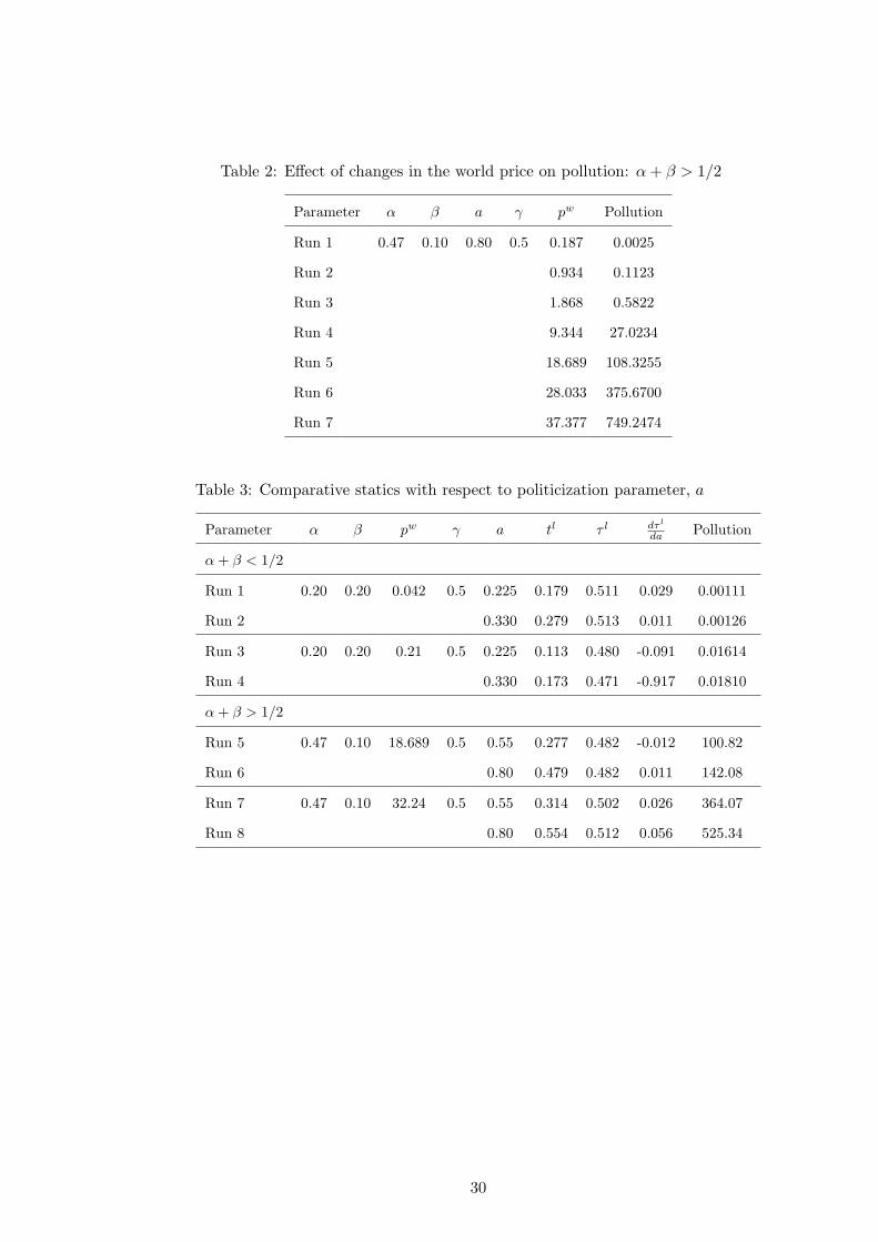
Table 2: Effect of changes in the world price on pollution: α + β > 1/2

Parameter α β a γ pw Pollution

Run 1 0.47 0.10 0.80 0.5 0.187 0.0025

Run 2 0.934 0.1123

Run 3 1.868 0.5822

Run 4 9.344 27.0234

Run 5 18.689 108.3255

Run 6 28.033 375.6700

Run 7 37.377 749.2474

Table 3: Comparative statics with respect to politicization parameter, a

Parameter α β pw γ a tl τ l dτ l

da Pollution

α + β < 1/2

Run 1 0.20 0.20 0.042 0.5 0.225 0.179 0.511 0.029 0.00111

Run 2 0.330 0.279 0.513 0.011 0.00126

Run 3 0.20 0.20 0.21 0.5 0.225 0.113 0.480 -0.091 0.01614

Run 4 0.330 0.173 0.471 -0.917 0.01810

α + β > 1/2

Run 5 0.47 0.10 18.689 0.5 0.55 0.277 0.482 -0.012 100.82

Run 6 0.80 0.479 0.482 0.011 142.08

Run 7 0.47 0.10 32.24 0.5 0.55 0.314 0.502 0.026 364.07

Run 8 0.80 0.554 0.512 0.056 525.34

30