School of Electrical, Electronic & Computer Engineering

Interactive Synthesis of Asynchronous Systemsbased on Partial Order Semantics

Agnes Madalinski

Technical Report Series

NCL-EECE-MSD-TR-2006-112

February 2006

Contact:

a.a.madalinski@ncl.ac.uk

EPSRC supports this work via GR/M94366 (MOVIE) and GR/R16754 (BESST).

NCL-EECE-MSD-TR-2006-112

Copyright c© 2006 University of Newcastle upon Tyne

School of Electrical, Electronic & Computer Engineering,

Merz Court,

University of Newcastle upon Tyne,

Newcastle upon Tyne, NE1 7RU, UK

http://async.org.uk/

University of Newcastle upon Tyne

School of Electrical, Electronic and Computer Engineering

Interactive Synthesis of Asynchronous Systems

based on Partial Order Semantics

by

A. Madalinski

PhD Thesis

May 2005

To my Mother

Contents

List of Figures v

List of Tables viii

List of Algorithms ix

Acknowledgements x

Abstract xi

1 Introduction 11.1 Asynchronous vs. synchronous . . . . . . . . . . . . . . . . . . . . . . . 11.2 Control signalling . . . . . . . . . . . . . . . . . . . . . . . . . . . . . . . 51.3 Data path . . . . . . . . . . . . . . . . . . . . . . . . . . . . . . . . . . . 71.4 Delay models . . . . . . . . . . . . . . . . . . . . . . . . . . . . . . . . . 101.5 Synthesis of control logic . . . . . . . . . . . . . . . . . . . . . . . . . . . 161.6 Motivation for this work . . . . . . . . . . . . . . . . . . . . . . . . . . . 181.7 Main contribution of this work . . . . . . . . . . . . . . . . . . . . . . . 201.8 Organisation of thesis . . . . . . . . . . . . . . . . . . . . . . . . . . . . 21

2 Formal models 232.1 Petri Nets . . . . . . . . . . . . . . . . . . . . . . . . . . . . . . . . . . . 23

2.1.1 Enabling and �ring . . . . . . . . . . . . . . . . . . . . . . . . . . 262.1.2 Petri net properties . . . . . . . . . . . . . . . . . . . . . . . . . . 272.1.3 Subclasses of Petri nets . . . . . . . . . . . . . . . . . . . . . . . 28

i

2.2 Signal Transition Graphs and State Graphs . . . . . . . . . . . . . . . . 292.2.1 Signal Transition Graphs . . . . . . . . . . . . . . . . . . . . . . 302.2.2 State Graphs . . . . . . . . . . . . . . . . . . . . . . . . . . . . . 322.2.3 Signal Transition Graph properties . . . . . . . . . . . . . . . . . 32

2.3 Branching processes . . . . . . . . . . . . . . . . . . . . . . . . . . . . . 352.3.1 Con�gurations and cuts . . . . . . . . . . . . . . . . . . . . . . . 392.3.2 Complete pre�xes of PN unfoldings . . . . . . . . . . . . . . . . . 412.3.3 LPN branching processes . . . . . . . . . . . . . . . . . . . . . . 43

3 Logic synthesis 463.1 Related work . . . . . . . . . . . . . . . . . . . . . . . . . . . . . . . . . 463.2 Implementation as logic circuit . . . . . . . . . . . . . . . . . . . . . . . 493.3 State-based logic synthesis . . . . . . . . . . . . . . . . . . . . . . . . . . 503.4 Synthesis example . . . . . . . . . . . . . . . . . . . . . . . . . . . . . . 513.5 State encoding problem . . . . . . . . . . . . . . . . . . . . . . . . . . . 54

4 Detection of encoding con�icts 604.1 Approximate state covering approach . . . . . . . . . . . . . . . . . . . . 60

4.1.1 Necessary condition . . . . . . . . . . . . . . . . . . . . . . . . . 624.1.2 Re�nement by partial state construction . . . . . . . . . . . . . . 65

4.2 Implementation . . . . . . . . . . . . . . . . . . . . . . . . . . . . . . . . 664.2.1 Collision stable conditions . . . . . . . . . . . . . . . . . . . . . . 674.2.2 ON-set of a collision relation . . . . . . . . . . . . . . . . . . . . 694.2.3 Overall procedure . . . . . . . . . . . . . . . . . . . . . . . . . . 734.2.4 Reducing the number of fake con�icts . . . . . . . . . . . . . . . 76

4.3 Experimental results . . . . . . . . . . . . . . . . . . . . . . . . . . . . . 794.4 Conclusions . . . . . . . . . . . . . . . . . . . . . . . . . . . . . . . . . . 82

5 Visualisation and resolution of encoding con�icts 845.1 Compact representation of con�icts . . . . . . . . . . . . . . . . . . . . . 855.2 Net transformation for resolution of con�icts . . . . . . . . . . . . . . . . 92

5.2.1 Validity . . . . . . . . . . . . . . . . . . . . . . . . . . . . . . . . 93

ii

5.2.2 Concurrency reduction . . . . . . . . . . . . . . . . . . . . . . . . 955.2.3 Signal insertion . . . . . . . . . . . . . . . . . . . . . . . . . . . . 97

5.2.3.1 Transition splitting . . . . . . . . . . . . . . . . . . . . 975.2.3.2 Concurrent insertion . . . . . . . . . . . . . . . . . . . . 100

5.3 Resolution concept . . . . . . . . . . . . . . . . . . . . . . . . . . . . . . 1015.3.1 X cores elimination: a general approach . . . . . . . . . . . . . . 1025.3.2 X core elimination by signal insertion . . . . . . . . . . . . . . . 104

5.3.2.1 Single signal insertion . . . . . . . . . . . . . . . . . . . 1045.3.2.2 Dual signal insertion (�ip �op insertion) . . . . . . . . . 108

5.3.3 X core elimination by concurrency reduction . . . . . . . . . . . 1115.3.4 Resolution constraints . . . . . . . . . . . . . . . . . . . . . . . . 114

5.4 Resolution process . . . . . . . . . . . . . . . . . . . . . . . . . . . . . . 1175.4.1 Manual resolution . . . . . . . . . . . . . . . . . . . . . . . . . . 118

5.4.1.1 Transformation condition . . . . . . . . . . . . . . . . . 1195.4.1.2 Resolution examples . . . . . . . . . . . . . . . . . . . . 120

5.4.2 Automated resolution . . . . . . . . . . . . . . . . . . . . . . . . 1255.4.3 Cost function . . . . . . . . . . . . . . . . . . . . . . . . . . . . . 126

5.5 Tool ConfRes: CSC con�ict resolver . . . . . . . . . . . . . . . . . . . 1315.5.1 Applied visualisation method . . . . . . . . . . . . . . . . . . . . 1315.5.2 Description . . . . . . . . . . . . . . . . . . . . . . . . . . . . . . 1335.5.3 Implementation . . . . . . . . . . . . . . . . . . . . . . . . . . . . 136

5.6 Conclusion . . . . . . . . . . . . . . . . . . . . . . . . . . . . . . . . . . . 140

6 Interactive synthesis 1416.1 VME-bus controller . . . . . . . . . . . . . . . . . . . . . . . . . . . . . . 1416.2 Weakly synchronised pipelines . . . . . . . . . . . . . . . . . . . . . . . . 1456.3 Phase comparator . . . . . . . . . . . . . . . . . . . . . . . . . . . . . . . 1476.4 AD converter . . . . . . . . . . . . . . . . . . . . . . . . . . . . . . . . . 149

6.4.1 Top level controller . . . . . . . . . . . . . . . . . . . . . . . . . . 1506.4.2 Scheduler . . . . . . . . . . . . . . . . . . . . . . . . . . . . . . . 154

6.5 D-element . . . . . . . . . . . . . . . . . . . . . . . . . . . . . . . . . . . 157

iii

6.6 Handshake decoupling element . . . . . . . . . . . . . . . . . . . . . . . 1606.7 GCD . . . . . . . . . . . . . . . . . . . . . . . . . . . . . . . . . . . . . . 1656.8 Conclusion . . . . . . . . . . . . . . . . . . . . . . . . . . . . . . . . . . . 172

7 Conclusion 1757.1 Summary . . . . . . . . . . . . . . . . . . . . . . . . . . . . . . . . . . . 1757.2 Areas of further research . . . . . . . . . . . . . . . . . . . . . . . . . . . 179

Bibliography 181

iv

List of Figures

1.1 Signalling protocols . . . . . . . . . . . . . . . . . . . . . . . . . . . . . . 61.2 Single-rail protocol . . . . . . . . . . . . . . . . . . . . . . . . . . . . . . 81.3 Four-phase dual-rail . . . . . . . . . . . . . . . . . . . . . . . . . . . . . 91.4 Two-phase dual-rail . . . . . . . . . . . . . . . . . . . . . . . . . . . . . . 101.5 Hu�man circuit model . . . . . . . . . . . . . . . . . . . . . . . . . . . . 121.6 Illustration of delay models . . . . . . . . . . . . . . . . . . . . . . . . . 131.7 Micropipeline structure . . . . . . . . . . . . . . . . . . . . . . . . . . . . 15

2.1 An example: a PN and its RG, an STG, its SG and its unfolding pre�x 252.2 Example: An illustration of a �ring rule . . . . . . . . . . . . . . . . . . 262.3 Examples of subclasses of PN systems . . . . . . . . . . . . . . . . . . . 292.4 A PN and one of �nite and complete pre�xes of its unfoldings . . . . . . 38

3.1 Overview of approaches for STG-based logic synthesis . . . . . . . . . . 473.2 Design �ow for asynchronous control circuits . . . . . . . . . . . . . . . . 503.3 VME-bus controller . . . . . . . . . . . . . . . . . . . . . . . . . . . . . . 523.4 CSC re�nement . . . . . . . . . . . . . . . . . . . . . . . . . . . . . . . 523.5 Read cycle VME-bus controller implementation . . . . . . . . . . . . . . 533.6 Approach overview for the resolution of the CSC problem . . . . . . . . 55

4.1 An example for the approximation technique . . . . . . . . . . . . . . . 644.2 Traversing a node . . . . . . . . . . . . . . . . . . . . . . . . . . . . . . . 694.3 Deriving the ON-set . . . . . . . . . . . . . . . . . . . . . . . . . . . . . 724.4 Reduction of a marked region by procedure reduceSlice . . . . . . . . . . 73

v

4.5 Detection of state coding con�icts . . . . . . . . . . . . . . . . . . . . . . 774.6 STG unfoldings with di�erent initial markings . . . . . . . . . . . . . . . 78

5.1 Visualisation of CSC con�icts . . . . . . . . . . . . . . . . . . . . . . . . 865.2 Visualisation examples of X cores . . . . . . . . . . . . . . . . . . . . . . 875.3 Visualisation of normalcy violation . . . . . . . . . . . . . . . . . . . . . 915.4 Concurrency reduction U n

99K t . . . . . . . . . . . . . . . . . . . . . . . 965.5 Transition splitting . . . . . . . . . . . . . . . . . . . . . . . . . . . . . . 975.6 Concurrent insertion v →n→ w . . . . . . . . . . . . . . . . . . . . . . . . 1005.7 Strategies for eliminating X cores . . . . . . . . . . . . . . . . . . . . . . 1035.8 X core elimination by signal insertion . . . . . . . . . . . . . . . . . . . 1055.9 Example: elimination of CSC cores in sequence . . . . . . . . . . . . . . 1055.10 Example: elimination of CSC cores in concurrent parts . . . . . . . . . . 1065.11 Example: elimination of CSC cores in choice branches . . . . . . . . . . 1075.12 Strategies for X core elimination . . . . . . . . . . . . . . . . . . . . . . 1085.13 Strategy for �ip �op insertion . . . . . . . . . . . . . . . . . . . . . . . . 1095.14 Example: �ip �op insertion . . . . . . . . . . . . . . . . . . . . . . . . . 1105.15 X core elimination by concurrency reduction . . . . . . . . . . . . . . . . 1125.16 Elimination of type I CSC cores . . . . . . . . . . . . . . . . . . . . . . . 1135.17 Elimination of type II CSC cores . . . . . . . . . . . . . . . . . . . . . . 1145.18 Visualisation of encoding con�icts . . . . . . . . . . . . . . . . . . . . . . 1155.19 Intersection of CSC cores . . . . . . . . . . . . . . . . . . . . . . . . . . 1165.20 N-normalcy violation for signal b . . . . . . . . . . . . . . . . . . . . . . 1175.21 The resolution process of encoding con�icts . . . . . . . . . . . . . . . . 1185.22 CSC con�ict resolution . . . . . . . . . . . . . . . . . . . . . . . . . . . . 1215.23 Normalcy con�ict resolution . . . . . . . . . . . . . . . . . . . . . . . . . 1235.24 Logic decomposition (d+ b): signal insertion n+

1 →oa− and n−1 →on+0 . . 124

5.25 Overview: automated resolution process . . . . . . . . . . . . . . . . . . 1265.26 Visualisation of encoding con�ict: an example . . . . . . . . . . . . . . . 1325.27 ConfRes dependencies . . . . . . . . . . . . . . . . . . . . . . . . . . . 1335.28 Interaction with ConfRes: an example . . . . . . . . . . . . . . . . . . 135

vi

6.1 VME-bus controller: read cycle . . . . . . . . . . . . . . . . . . . . . . . 1426.2 Selected equations . . . . . . . . . . . . . . . . . . . . . . . . . . . . . . 1446.3 Weakly synchronised pipelines . . . . . . . . . . . . . . . . . . . . . . . . 1466.4 Phase comparator . . . . . . . . . . . . . . . . . . . . . . . . . . . . . . . 1486.5 Block diagram of the AD converter . . . . . . . . . . . . . . . . . . . . . 1496.6 STG transformation of the top level controller . . . . . . . . . . . . . . . 1516.7 Valid transformations for top level controller . . . . . . . . . . . . . . . . 1536.8 STG transformation of the scheduler . . . . . . . . . . . . . . . . . . . . 1546.9 Logic equations . . . . . . . . . . . . . . . . . . . . . . . . . . . . . . . . 1556.10 Resolution attempts for the scheduler . . . . . . . . . . . . . . . . . . . . 1556.11 D-element . . . . . . . . . . . . . . . . . . . . . . . . . . . . . . . . . . . 1586.12 Handshake decoupling element . . . . . . . . . . . . . . . . . . . . . . . 1616.13 Handshake decoupling element: �nal implementation . . . . . . . . . . . 1646.14 Implementation of the decomposed �ip �op solution . . . . . . . . . . . 1656.15 GCD . . . . . . . . . . . . . . . . . . . . . . . . . . . . . . . . . . . . . . 1676.16 Equations for GCD controller obtained by Petrify . . . . . . . . . . . 1686.17 Resolution process of GCD controller . . . . . . . . . . . . . . . . . . . . 1696.18 Equations for GCD controller obtained by ConfRes . . . . . . . . . . . 1716.19 Complex gates implementation of GCD controller (sequential solution) . 172

7.1 Applications of interactive re�nement of CSC con�icts . . . . . . . . . . 177

vii

List of Tables

4.1 Necessary condition . . . . . . . . . . . . . . . . . . . . . . . . . . . . . . 804.2 Size of the traversed state space . . . . . . . . . . . . . . . . . . . . . . . 814.3 Number of fake con�icts . . . . . . . . . . . . . . . . . . . . . . . . . . . 814.4 Reduction of collisions . . . . . . . . . . . . . . . . . . . . . . . . . . . . 82

6.1 Possible single signal insertions . . . . . . . . . . . . . . . . . . . . . . . 1446.2 Comparison: automatic and manual re�nement . . . . . . . . . . . . . . 172

viii

List of Algorithms

1 Identifying collision stable conditions . . . . . . . . . . . . . . . . . . . . 682 Procedure to traverse an event . . . . . . . . . . . . . . . . . . . . . . . 703 Procedure to traverse a condition . . . . . . . . . . . . . . . . . . . . . . 714 Constructing the ON-set of a collision relation . . . . . . . . . . . . . . . 715 Setting the ��rst� min-cuts for c . . . . . . . . . . . . . . . . . . . . . . . 746 Reducing slice . . . . . . . . . . . . . . . . . . . . . . . . . . . . . . . . . 747 Detecting state coding con�icts by STG unfolding . . . . . . . . . . . . . 758 Resolution of encoding con�icts . . . . . . . . . . . . . . . . . . . . . . . 1379 Computation of possible transformations . . . . . . . . . . . . . . . . . 13710 Computation of valid transformations (phase one) . . . . . . . . . . . . . 139

ix

Acknowledgements

This work would not have been possible without intensive collaboration with manypeople. I would like to express my gratitude to my supervisor, Alex Yakovlev, forintroducing me to the ideas of asynchronous circuit design and for supporting me duringmy research.

Most of the ideas described in this thesis are a result of numerous discussions withAlex Bystrov, Victor Khomenko and, of course, my supervisor. I would also like tothank my fellow PhD students, especially Imam Kistijantoro and Danil Sokolov, whobeen very helpful whenever I needed advice and information about all sorts of practicalquestions.

In addition, I would like to thank Margie Craig for reading through the whole PhDthesis and helping me with my English.

Finally, I would like to acknowledge that this work was supported by the EPSRCprojects MOVIE (grant GR/M94366) and BESST (grant GR/R16754) at the Universityof Newcastle upon Tyne.

x

Abstract

An interactive synthesis of asynchronous circuits from Signal Transition Graphs (STGs)based on partial order semantics is presented. In particular, the fundamental problemof encoding con�icts in the synthesis is tackled, using partial orders in the form of STGunfolding pre�xes. They o�er a compact representation of the reachable state spaceand have the added advantage of simple structures.

Synthesis of asynchronous circuits from STGs involves resolving state encoding con-�icts by re�ning the STG speci�cation. The re�nement process is generally done auto-matically using heuristics. It often produces sub-optimal solutions, or sometimes failsto solve the problem, then requiring manual intervention by the designer. A frameworkfor an interactive re�nement process is presented, which aims to help the designer tounderstand the encoding problems. It is based on the visualisation of con�ict cores,i.e. sets of transitions causing encoding con�icts, which are represented at the level of�nite and complete pre�xes of STG unfoldings. The re�nement includes a number ofdi�erent transformations giving the designer a larger design space as well as applyingto di�erent levels of interactivity. This framework is intended to work as an aid to theestablished state-based synthesis. It also contributes to an alternative synthesis basedon unfolding pre�xes rather than state graphs.

The proposed framework has been applied to a number of design examples to demon-strate its e�ectiveness. They show that the combination of the transparent synthesistogether with the experience of the designer makes it possible to achieve tailor-madesolutions.

xi

Chapter 1

Introduction

Asynchronous circuits design has been an active research area since the early daysof digital circuit design, but only during the last decade has there been a revival inthe research on asynchronous circuits [1, 2, 83]. Up until now, asynchronous circuitshave only been applied commercially as small sub-circuits, often as peripherals to con-trollers. Examples [24] include counters, timers, wake-up circuits, arbiters, interruptcontrollers, FIFOs, bus controllers, and interfaces. The need for such asynchronouscircuits stems largely from intrinsically asynchronous speci�cations. Emphasis is nowshifting from small asynchronous sub-circuits to asynchronous VLSI circuits and sys-tems. Asynchronous VLSI is now progressing from a fashionable academic researchtopic to a viable solution to a number of digital VLSI design challenges.

This chapter brie�y outlines the motivation and basic concept of asynchronous cir-cuit design. A number of works, e.g. [9, 21, 30, 75, 98], provide a more extensiveintroduction to, and comparison of, the most common approaches. This chapter alsodescribes the main contribution and the organisation of this thesis.

1.1 Asynchronous vs. synchronous

The majority of the digital circuits designed and manufactured today are synchronous.In essence, they are based on two assumptions which greatly simplify their design.Firstly, all signals are assumed binary where simple Boolean logic can be used to de-

1

scribe and manipulate logic constructs. Secondly, all components share a common anddiscrete notation of time, as de�ned by a clock signal distributed throughout the circuit.However, asynchronous circuits are fundamentally di�erent. They also assume binarysignals, but there is no common and discrete time. Instead the circuits use handshakingbetween their components in order to perform the necessary synchronisation, communi-cation and sequencing operations. This di�erence gives asynchronous circuits inherentproperties as listed below. A further introduction to the advantages mentioned belowcan be found in [5].

� Power e�ciencyThe power consumption of high performance synchronous circuits is related tothe clock, which signal propagates to every operational block of the circuit eventhough many parts of the circuit are functionally idle. Thus energy is wasted ondriving the clocked inputs of these gates which do not perform any useful actions.In contrast, an asynchronous circuit only consumes energy when and where it isactive. Any sub-circuit is quiescent until activated. After completion of its task,it returns to a quiescent state until a next activation. However, it is not obvi-ous to what extent this advantage is fundamentally asynchronous. Synchronoustechniques such as clock gating may achieve similar bene�ts, but have their limi-tations.

� PerformanceIn a synchronous circuit all the computation must be completed before the endof the current cycle, otherwise an unstable and probably incorrect signal valuemay be produced. To guarantee the correct operation of synchronous circuitsit is mandatory to �nd out the propagation times through all the paths in thecombinational gates, assuming any possible input pattern. Then the length of theclock cycle must be longer than the worst propagation delay. This �xed cycle timerestricts the performance of the system.In an asynchronous circuit the next computation step can start immediately afterthe previous step has been completed. There is no need to wait for a transition of

2

the clock signal. This leads, potentially, to a fundamental performance advantagefor asynchronous circuits, an advantage that increases with the variability in delaysassociated with these computation steps.

� Clock skewReliable clock distribution is a big problem in complex VLSI chips because of theclock skew e�ect. This is caused by variations in wiring delays to di�erent parts ofthe chip. It is assumed that the clock signal reaches the di�erent stages of the chipsimultaneously. However, as chips get more complex and logic gates reduced insize, the ratio between gate delays and wire delays changes so that latter begin tosigni�cantly a�ect the operation of the circuit. In addition, clock wiring can takemore than half of all the wiring in a chip. By choosing an asynchronous imple-mentation the designer escapes the clock skew problem and the associated routingproblem. Although asynchronous circuits can also be subject to the greater e�ectof wire delays; those problems are solved at a much more local level.

� Electromagnetic compatibility (EMC)The clock signal is a major cause of electromagnetic radiation emissions, which arewidely regarded as a health hazard or source of interference, and are becomingsubject to strict legislation in many countries. EMC problems are caused byradiation from the metal tracks that connect the clocked chip to the power supplyand target devices, and from the fact that on-chip switching activity tends to beconcentrated towards the end of the clock cycle. These strong emissions, beingharmonics of the clock frequency, may severely a�ect radio equipment. Due tothe absence of a clock, asynchronous circuits have a much better energy spectrumthan synchronous circuits. The spectrum is smoother and the peak values arelower due to irregular computation and communication patterns.

� ModularityIn a synchronous circuit all its computational modules are driven by one basicclock (or a few clocks rationally related to each other), and hence must work at a�xed speed rate. If any functional unit is redesigned and substituted by a faster

3

unit no direct increase in performance will be achieved unless the clock frequencyis increased in order to match the shorter delay of the newly introduced unit. Theincreased clock speed, however, may require the complete redesign of the wholesystem.Asynchronous circuits, however, are typically designed on the basis of explicit self-timed protocols. Any functional unit can be correctly substituted by another unitimplementing the same functionality and following the same protocol but with adi�erent performance. Hence asynchronous circuits achieve better plug and playcapabilities.

� MetastabilityAll synchronous chips interact with the outside world, e.g. via interrupt signals.This interaction is inherently asynchronous. A synchronisation failure may occurwhen an unstable synchronous signal is sampled by a clock pulse into a memorylatch. Due to the dynamic properties of an electronic device that contains inter-nal feedback, the latch may, with nonzero probability, hang in a metastable state(somewhere in between logical 0 and 1 ) for a theoretically inde�nite period oftime. Although in practice this time is always bounded, it is much longer thanthe clock period. As a result, the metastable state may cause an unpredictableinterpretation in the adjacent logic when the next clock pulse arrives. Most asyn-chronous circuits wait until metastability is resolved. Even though in some realtime application this may still cause failure, the probability is very much lowerthan in synchronous systems, which must trade o� reliability against speed.

On the other hand there are also some drawbacks. Primary, asynchronous circuits aremore di�cult to design in an ad hoc fashion than synchronous circuits. In a synchronoussystem, a designer can simply de�ne the combinational logic necessary to compute thegiven functions, and surround it with latches. By setting the clock rate to a long enoughperiod, worries about hazards (undesired signal transitions) and the dynamic state ofthe circuit are removed. In contrast, designers of asynchronous systems must pay at-tention to the dynamic state of the circuit. To avoid incorrect results hazards must be

4

removed from the circuit, or not introduced in the �rst place. The predominance ofCAD tools orientated towards synchronous systems makes it di�cult to design complexasynchronous systems. However, most circuit simulation techniques are independentof synchrony, and existing tools can be adapted for asynchronous use. Also, there areseveral methodologies and CAD tools developed speci�cally for asynchronous design.Some of them are discussed later. Another obstacle is that asynchronous design tech-niques are not typically taught in universities. If a circuit design company decides touse an asynchronous logic it has to train its engineering sta� in the basics.

Finally, the asynchronous control logic that implements the handshaking normallyrepresents an overhead in terms of silicon area, circuit speed, and power consumption.It is therefore pertinent to ask whether or not the investment pays o�, i.e. whetherthe use of asynchronous techniques result in a substantial improvement in one or moreof the above areas. In spite of the drawbacks, there exist several commercial asyn-chronous designs which bene�t from the advantages listed above. Such designs includethe Amulet microprocessors developed at the University of Manchester [28], a con-tactless smart card chip developed at Philips [35], a Viterbi decoder developed at theUniversity of Manchester [88], a data driven multimedia processor developed at Sharp[101], and a �exible 8-bit asynchronous microprocessor developed at Epson [34].

1.2 Control signalling

Asynchronous circuits do not use clocks and therefore synchronisation must be donein a di�erent way. One of the main paradigms in asynchronous circuits is distributedcontrol. This means that each unit synchronises only with those units for which thesynchronisation is relevant and at the time when synchronisation takes place, regardlessof the activities carried out by other units in the same circuit. For this reason, asyn-chronous functional units incorporate explicit signals for synchronisation that executesome handshake protocol with their neighbours. For example, let there be two units, asender A and a receiver B, as shown in Figure 1.1(a). A request is sent from A to B toindicate that A is requesting some action from B. When B has either done the action or

5

has stored the request, it acknowledges the request by sending the acknowledge signal,which is sent from B to A. To operate in this manner, data path units commonly havetwo signals, request and acknowledge used for synchronisation. The request signal is aninput signal used by the environment to indicate that input data are ready and that anoperation is requested to the unit. The output signal, the acknowledge signal, is usedby the unit to indicate that the requested operation has been completed and that theresult can be read by the environment.

The purpose of an asynchronous control circuit is to interface a portion of datapath to its sources and sinks of data. The controller manages all the synchronisationrequirements, making sure that the data path receives its input data, performs theappropriate computations when they are valid and stable, and that the results aretransferred to the receiving blocks whenever they are ready.

The most commonly used handshake protocols are the four-phase and two-phaseprotocol.

Sender AReq

AckReceiver B

(a) handshaking

Ack

Req

start event ievent i done

start event i+1ready for next event

(b) four-phase

Ack

Req

start event ievent i done

event i+1 donestart event i+1

(c) two-phase

Figure 1.1: Signalling protocols

Four-phase protocol The four-phase protocol also called return-to-zero (RZ) isshown in Figure 1.1(b). The waveforms appear periodic for convenience but they do notneed to be so in practice. The curved arrows indicate the required before/after sequenceof events. There are no implicit assumptions about the delay between successive events.Note that in this protocol there are typically four transitions (two on the request and

6

two on the acknowledgement) required to complete a particular event transition.

Two-phase protocols The two-phase protocol, also called non-return-to-zero (NRZ),is shown in Figure 1.1(c). The waveforms are the same as for four-phase signalling withthe exception that every transition on the request wire, both falling and rising, indicatesa new request. The same is true for transition on the acknowledgement wire.

Proponents of the four-phase signalling scheme argue that typically four-phase circuitsare smaller than they are for two-phase signalling, and that the time required for thefalling transition on the request and on the acknowledge lines do not usually causeperformance degradation. This is because falling transitions happened in parallel withother circuit operations. Two-phase proponents argue that two-phase signalling is bet-ter from both a power and a performance standpoint, since every transition representsa meaningful event and no transitions or power are consumed in the return-to-zero,because there is no resetting of the handshake link. Whilst this is true, in principle, itis also the case that most two-phase interface implementations require more logic thatfour-phase equivalents.

Other interface protocols, based on similar sequencing rules, exist for three or moremodule interfaces. A particular common design requirement is to conjoin two or morerequests to provide a single outgoing request, or conversely to provide a conjunctionof acknowledge signals. A commonly used asynchronous element is the C-element [73],which can be viewed as a protocol preserving conjunctive gate. The C-element e�ectivelymerges two requests into a single request and permits three subsystems to communicatein a protocol preserving two- or four-phase manner.

1.3 Data path

The previous section only addressed control signals. There are also several approachesto encoding data. The most common are the single- and dual-rail protocols.

7

Single-rail protocol The single-rail protocol, also referred to as bundled-data proto-col, uses either two- or four-phase signalling to encode data. In this case, for an n-bitdata value to be passed from sender to receiver, n+2 wires will be required (n bits ofdata, one request bit and one acknowledge bit), see Figure 1.2(a). The data signals arebundled with the request and acknowledgement. This type of data encoding containsan implied timing assumption, namely the assumption that the propagation times ofcontrol and data are either equal, or that the control propagates slower than the datasignals.

Ack

Req

Sender Receiver

nData

(a) channel

Ack

Req

Data

(b) four-phase

Ack

Req

Data

(c) two-phase

Figure 1.2: Single-rail protocol

The four-phase protocol is illustrated in Figure 1.2(b). The term four-phase refersto the number of communication actions. First, the sender issues data and sets requesthigh, then the receiver absorbs the data and sets acknowledge high. The sender respondsby taking request low, at which point data is no longer guaranteed to be valid. Finally,the receiver acknowledges this by taking acknowledge low. At this point the sender mayinitiate the next communication cycle.

Dual-rail protocol A common alternative to the single-rail approach is dual-railencoding. The request signal is encoded into the data signal using two wires per bitof information. For an n-bit data value the sender and receiver must contain 3n wires:

8

two wires for each bit of data and the associated request, plus another bit for theacknowledge. An improvement on this protocol is possible when n-bits of data areconsidered to be associated in every transition, as in the case when the circuit operateson bytes or words. Then it is convenient to combine the acknowledges into a single wire.The wiring complexity is reduced to 2n + 1 wires: 2n for the data and an additionalacknowledge signal.

The four-phase dual-rail protocol, shown in Figure 1.3(a), is in essence a four-phaseprotocol using two request wires per bit of information, d; one wire d.t is used for sig-nalling a logic true, and another d.f is used for signalling a logic false. When observinga 1 -bit channel one will see a sequence of four-phase handshakes where the participatingrequest signal in any handshake cycle can be either d.t or d.f . This protocol is veryrobust, because two parties can communicate reliably regardless of delays in the wiresconnecting the two parties, thus the protocol is delay-insensitive.

Sender Receivern

Ack

Data, Req

(a) channel

d.f

Not used

Valid 1

Valid 0

Empty

1 1

1 0

10

0 0

d.t

(b) encoding

Valid Empty Valid

Ack

Data {d.t, d.f} Empty

(c) waveforms

Figure 1.3: Four-phase dual-rail

The encoding is presented in Figure 1.3(b). It has four codewords: two valid code-words (representing logic true and logic false), one idle and one illegal codeword. Ifthe sender issues a valid codeword, then the receiver absorbs the codeword and setsacknowledge high. The sender responds by issuing the empty codeword, which is thenacknowledged by the receiver, by taking the acknowledge low. At this point the sendermay initiate the next communication cycle. This process is illustrated in Figure 1.3(c).An abstract view is a data stream of valid codewords separated by empty ones.

9

The two-phase dual-rail protocol also uses two wires per bit, but the informationis encoded as events (transitions). On an n-bit channel a new codeword is receivedwhen exactly one wire in each of the n wire pairs has made a transition. There isno empty value. A valid message is acknowledged and followed by another messagethat is acknowledged. Figure 1.4 shows the signal waveforms on a 2 -bit channel usingtwo-phase dual-rail protocol.

Sender Receiver

Ack

(d1.t, d1.f)

(d0.t, d0.f)

(a) channel

d0.fd0.t

d1.fd1.t

Ack

00 01 00 11

(b) waveforms

Figure 1.4: Two-phase dual-rail

There exist other communication protocols such as 1-of-n encodings used in controllogic and higher-radix data encodings. If the focus is on communication rather thencomputation, m-of-n encodings may be of relevance.

1.4 Delay models

Asynchronous design methodologies are classi�ed by the delay models which they as-sume on gates, wires and feedback elements in the circuit. There are two fundamentalmodels of delay, the pure delay model and the inertial delay model. A pure delay modelcan delay the propagation of a waveform, but does not otherwise alter it. An inertialdelay can alter the shape of a waveform by attenuating short glitches. More formally,an inertial delay has a threshold period. Pulses of a duration less then the thresholdperiod are �ltered out.

Delays are also characterised by their timing models. In a �xed delay model, a delayis assumed to have a �xed value. In a bounded delay model, a delay may have any value

10

in a given time interval. In unbounded delay model, a delay may take on any �nitevalue.

An entire circuit's behaviour can be modelled on the basis of its component model. Ina gate-level model each gate and primitive component in the circuit has a correspondingdelay. In a complex-gate model, an entire sub-network of gates is modelled by a singledelay, that is, the network is assumed to behave as a single operator, with no internaldelays. Wires between gates are also modelled by delays. A circuit model is thus de�nedin terms of the delay models for the individual wires and components. Typically, thefunctionality of a gate is modelled by an instantaneous operator with an attached delay.

Given the circuit model, it is also important to characterise the interaction of thecircuit with its environment. The circuit and its environment together form a closedsystem, called complete circuit. If the environment is allowed to respond to a circuit'soutputs without any timing constraints, the two interact in input/output mode. Oth-erwise, environmental timing constraints are assumed. The most common example isfundamental mode where the environment must wait for a circuit to stabilise beforeresponding to circuit outputs.

This section introduces widely used models, and brie�y reviews the existing designmethodologies for each model.

Hu�man circuits The most obvious model to use for asynchronous circuits is thesame model used for synchronous circuits. Speci�cally, it is assumed that the delayin all circuit elements and wires is known, or at least bounded. Hu�man circuits aredesigned using a traditional asynchronous state machine approach. As illustrated inFigure 1.5, an asynchronous state machine has primary inputs, primary outputs, andfeed-back state variables. The state is stored in the feedback loop and thus may needdelay elements along the feedback path to prevent state changes from occurring toorapidly.

The design of Hu�man circuits begins with a speci�cation given in a �ow table [102]which can be derived using an asynchronous state machine. The goal of the synthesisprocedure is to divide a correct circuit netlist which has been optimised according to

11

Delay

CombinationalLogic

outputsinputs

Figure 1.5: Hu�man circuit model

design criteria such as area, speed, or power. The approach taken for the synthesis ofsynchronous state machines is to derive the synthesis problem into three steps. The �rststep is state minimisation, in which compatible states are merged to produce a simple�ow table. The second step is state assignment in which a binary encoding is assignedto each state. The third step is logic minimisation in which an optimised netlist isderived from an encoded �ow table. The design of Hu�man circuits can follow the samethree step process, but each step must be modi�ed to produce correct circuits under anasynchronous timing model.

Hu�man circuits are typically designed using the bounded gate delay and wire delaymodel. With this model, circuits are guaranteed to work, regardless of gate and wiredelays as long as a bound on the delays is known. In order to design correct Hu�mancircuits, it is also necessary to put some constraints on the behaviour of the environment,namely when inputs are allowed to change. A number of di�erent restrictions on inputshave been proposed, each resulting in variations of the synthesis procedure. The �rstis single-input change (SIC), which states that only one input is allowed to change at atime. In other words, each input change must be separated by a minimum time interval.If the minimum time interval is set to be the maximum delay for the circuit to stabilise,the restriction is called single-input change fundamental mode. This is quite restrictive,though, so another approach is to allow multiple-input changes (MIC). Again, if inputchanges are allowed only after the circuit stabilises, this mode of operation is calledmultiple-input change fundamental mode. An extended MIC model, referred to as burstmode [77], allows multiple inputs to change at any time as long as the input changesare grouped together in bursts.

12

Muller circuits Muller circuits [73] are designed under the unbounded gate delaymodel. Under this model, circuits are guaranteed to work regardless of gate delays,assuming that wire delays are negligible. This means that whenever a signal changesvalues, all gates it is connected to will see that change immediately. Such a model iscalled speed-independent (SI)[73] and is illustrated in Figure 1.6(a). A similar model,where only certain forks are isochronic forks is called quasi-delay insensitive (QDI)[67].This model is depicted in Figure 1.6(b). Isochronic forks [6] are forking wires where thedi�erence in delays between the branches is negligible.

delaygate delay

gate

delaygate

(a) SI

delaygate delay

gate

delaygate

delay

(b) QDI

delaygate

delaygate

delaygate delay

delay

delay

(c) DI

Figure 1.6: Illustration of delay models

Similar to the SI model is the self-timed model [92]. It contains a group of self-timedelements. Each element contains an equipotential region, where wires have negligible orwell-bounded delay. An element itself may be an SI circuit, or a circuit whose correctoperation relies on the use of local timing assumptions. However, no timing assumptionsare made on the communication between regions, i.e. , communication between regionsis delay-insensitive.

Muller circuit design requires explicit knowledge of the behaviour allowed by theenvironment. It does not, however, put any restriction on the speed of the environment.The design of Muller circuits requires a somewhat di�erent approach as compared withtraditional sequential state machine design. Most synthesis methods for Muller circuitstranslate the higher-lever speci�cation into a state graph. Next, the state graph isexamined to determine if a circuit can be generated using only the speci�ed inputand output signals. If two states are found that have the same value of inputs andoutputs but lead through an output transition to di�erent next states, no circuits canbe produced directly. This ambiguity is known as an encoding con�ict. In this case,

13

either the protocol must be changed or new internal state signals must be added tothe design. The method of determining the necessary state variables is quite di�erentfrom that used for Hu�man circuits. Logic is derived using modi�ed versions of logicminimisation procedures. The modi�cations needed are based upon the technologythat is being used for implementation. Finally, the design must be mapped to gates ina given gate library. This last step requires a substantially modi�ed technology mappingprocedure as compared with traditional state machine synthesis methods.

Delay-insensitive circuits A delay-insensitive (DI) circuit assumes that delays inboth gates and wires are unbounded, Figure 1.6(c). This delay model is most realisticand robust with respect to manufacturing processes and environmental variations. Ifa signal fails to propagate at a particular point then the circuit will stop functioningrather than producing a spurious result.

The class of DI circuits is built out of simple gates and thus its operation is quitelimited. Only very few circuits can be designed to be completely DI. Therefore, DIimplementation is usually obtained from modules whose behaviour is considered to beDI on their interfaces.

Several DI methodologies have been proposed. They are usually obtained from aspeci�cation in a high-level programming language such as Communicating SequentialProcesses (CSP) [32] and Tangram [7]. The transformation from the speci�cation toimplementation, composed of common gates, is driven by the syntax and structure ofthe speci�cation itself.

Micropipelines Micropipelines [100] are an e�cient implementation of asynchronouspipelined modules. They were introduced as an alternative to synchronous elasticpipeline design, i.e. pipelines in which the amount of data contained can vary. However,they proved to be a very e�cient and fast implementation of arithmetic units, and havebeen used in micropipelined systems such as the Amulet microprocessor [28].

The methodology does not �t precisely in the delay model classi�cation, as it uses abundled data communication protocol moderated by a delay-insensitive control circuit[30].

14

C C

Ain

Rin

Rout

Aout

C

(a) control

Delay

C

C

Cd

Pd

P

Register

C

Cd

Pd

P

RegisterL

ogic

Log

ic

C

Cd

Pd

P

Register

C

Delay

Log

ic

Delay

C

Ain

Rin Aout

Rout

Din Dout

(b) computation

Figure 1.7: Micropipeline structure

The basic implementation structure for a micropipeline is the control �rst-in �rst-out queue (FIFO) shown in Figure 1.7(a), where the gates labelled C are C-elements,which are elements whose output is 1 when all inputs are 1, 0 when all inputs are 0,and hold their state otherwise. The FIFO stores transitions sent to it trough Rin, shiftsthem to the right, and eventually outputs them through Rout.

The simple transition FIFO can be used as the basis for a complete computationpipeline as shown in Figure 1.7(b). The register output Cd is a delayed version of inputC, and output Pd is a delayed version of input P . Thus, the transition FIFO in Figure1.7(a) is embedded in Figure 1.7(b), with delays added. The registers are initially active,passing data directly from data inputs to data outputs. When a transition occurs onthe C (capture) wire, data is no longer allowed to pass and the current values of theoutputs are statically maintained. Then, once a transition occurs on P (pass) input,data is again allowed to pass from input to output, and the cycle repeats. The logicblocks between registers perform computation on the data stored in a micropipeline.

15

Since these blocks slow down the data moving through them, the accompanying controltransition must also be delayed. This is done by adding delay elements.

1.5 Synthesis of control logic

There exist a number of approaches for the speci�cation and synthesis of asynchronouscircuits. They are based on state machines, Petri Nets (PNs) and high-level descriptionslanguages. State machines are the most traditional approach, where speci�cations aredescribed by a �ow table [102], and the synthesis is performed similar as in synchronoussystems. The main characteristic of such an approach is that it produces a sequentialmodel out of a possibly concurrent speci�cation, where concurrency is represented as aset of possible interleaving resulting in a problem with the size of the speci�cation. Inorder to specify concurrent systems PN [86] have been introduced. Rather than charac-terising system states, these describe partially ordered sequences of events. Methods forsynthesis based on PN can be divided in two categories. The �rst category comprisestechniques of direct mapping of PN constructs into logic, and the second category per-forms explicit logic synthesis from interpreted PNs. In high-level descriptions languagesthe system is speci�ed in a similar way to conventional programming languages. Mostof these languages are based on Communicating Sequential Processes (CSP) [32], whichallow concurrent system to be described in a abstract way by using channels as the pri-mary communication mechanism between sub-systems. The processes are transformedinto low-level process and mapped directly to a circuit.

Aspect of PN based synthesis is within the scope of this work, therefore the problemof the synthesis of control circuits from PN1 is outlined. PNs provide a simple graphicaldescription of the system with the representation of concurrency and choice. In order touse PNs to model asynchronous circuits, it is necessary to relate transitions to events onsignal wires. There have been several variants of PNs that accomplish this, including M-nets [91], I-nets [72], and change diagrams [46]. The most common are Signal TransitionGraphs (STGs)[12]. They are a particular type of labelled Petri nets, where transitionsare associated with the changes in the values of binary variables. These variables can,

1See next chapter for a formal de�nition of the PN theory.

16

for example, be associated with wires, when modelling interfaces between blocks, or withinput, output and internal signals in a control circuit. STGs can be extracted from ahigh-level Hardware Description Language (HDL) and timing diagrams, respectively,which are popular amongst hardware designers.

A state-based synthesis [14]2 can be applied to design asynchronous control cir-cuits from STGs. The key steps in this method are the generation of a state graph,which is a binary encoded reachability graph of the underlying Petri net, and derivingBoolean equations for the output signals via their next-state functions obtained from thestate graph. The state-based synthesis su�erers from problems of state space explosionand state assignment. The explicit representation of concurrency results in the stateexplosion problem. The state assignment problem arises when semantically di�erentreachable states of an STG have the same binary encoding. If this occurs, the systemis said to violate the Complete State Coding (CSC) property. Enforcing CSC is one ofthe most di�cult problems in the synthesis of asynchronous circuits from STGs.

While the state-based approach is relatively simple and well-studied, the issue ofcomputational complexity for highly concurrent STGs is quite serious due to the statespace explosion problem. This puts practical bounds on the size of control circuits thatcan be synthesised using such techniques. In order to alleviate this problem, Petri netanalysis techniques based on causal partial order semantics, in the form of Petri netunfoldings, are applied to circuit synthesis.

A �nite and complete unfolding pre�x of an STG is a �nite acyclic net which im-plicitly represents all the reachable states of its STG together with transitions enabledat those states. Intuitively, it can be obtained through �unfolding� the STG until iteventually starts to repeat itself and can be truncated without loss of information,yielding a �nite and complete pre�x. E�cient algorithms exist for building such pre-�xes. Complete pre�xes are often exponentially smaller than the corresponding stategraphs, especially for highly concurrent Petri nets, because they represent concurrencydirectly rather than by multidimensional `diamonds' as it is done in state graphs.

The unfolding-based synthesis avoids the construction of reachability graph of an2See Chapter 3 for a more formal de�nition of the state-based synthesis.

17

STG and instead use only structural information from its �nite and complete unfoldingpre�x. These informations are used in [93] to derive approximated Boolean covers andrecently in [42] they are used to build e�cient algorithm based on the IncrementalBoolean Satis�ability (SAT).

1.6 Motivation for this work

The explicit logic synthesis method based on state space exploration is implemented inthe Petrify tool [18]. It performs the process automatically, after �rst constructingthe reachability graph (in the form of a BDD [8]) of the initial STG speci�cation andthen, applying the theory of regions [19] to derive Boolean equations. An example ofits use was the design of many circuits for the AMULET-3 microprocessor [28]. Sincepopularity of this tool is steadily growing, it is likely that STGs and PNs will increasinglybe seen as an intermediate or back-end notation for the design of controllers.

During the synthesis the state assignment problem requires the re�nement of thespeci�cation. Petrify explores the underlying theory of regions to resolve the CSCproblem and relies on a set of optimisation heuristics. Therefore, it can often producesub-optimal solutions or sometimes fail to solve the problem in certain cases, e.g. whena controller speci�cation is de�ned in a compact way using a small number of signals.Such speci�cations often have CSC con�icts that are classi�ed as irreducible by Pet-rify. Therefore, manual design may be required for �nding good synthesis solutions,particularly in constructing interface controllers, where the quality of the solution iscritical for the system's performance.

According to a practising designer [87], a synthesis tool should o�er a way for thedesigner to understand the characteristic patterns of a circuit's behaviour and the causeof each encoding con�ict, in order to allow the designer to manipulate the model in-teractively by choosing how to re�ne the speci�cation and where in the speci�cation toperform transformations. State graphs distort the relationship of causality, concurrencyand con�ict and they are known to be large in size. Petrify o�ers a way to exhibitencoding con�icts by highlighting states in con�icts. However, all states which are in

18

con�ict are highlighted in the same way. The extraction of information from this modelis a di�cult task for human perception. Therefore, a visualisation method is needed tohelp the designer in understanding the causes of encoding con�icts. Moreover, a methodis needed which facilitates an interactive re�nement of an STG with CSC con�icts.

Alternative synthesis approaches avoid the construction of the reachable state space.Such approaches include techniques based on either structural analysis of STGs orpartial order techniques. The structural approach, e.g. in [11] performs graph-basedtransformations on the STG and deals with the approximated state space by means oflinear algebraic representations. The main bene�t of using structural methods is theability to deal with large and highly concurrent speci�cations, that cannot be tackled bystate-based methods. On the other hand, structural methods are usually conservativeand approximate, and can only be exact when the behaviour of the speci�cations isrestricted in some sense. The unfolding-based method represents the state space in theform of true concurrency (or partial order) semantics provided by PN unfoldings. Theunfolding-based approach in [93] demonstrates clear superiority in terms of memoryand time e�ciency for some examples. However, the approximation based approachcannot precisely ascertain whether the STG has a CSC con�ict without an expensivere�nement process. Therefore, an e�cient method for detection and resolution of CSCcon�ict in STG unfolding pre�xes is required.

The problem of interactive re�nement of CSC con�icts in the well established state-based synthesis can be tackled by employing STG unfolding pre�xes. They are well-suited for both the visualisation of STG's behaviour and alleviating the state spaceexplosion problem due to their compact representation of the state space in the form oftrue concurrency semantics. At the same time the CSC problem in the unfolding-basedsynthesis can be addressed resulting in an complete synthesis approach which avoidsthe construction of the state space.

19

1.7 Main contribution of this work

The main objective of this work is the introduction of transparency and interactivity inthe synthesis of asynchronous systems from Signal Transition Graphs (STGs). The qual-ity of the design of systems such as asynchronous interface controllers or synchronisers,which act as �glue logic� between di�erent processes, a�ects performance. Automatedsynthesis usually o�ers little or no feedback to the designer making it di�cult to in-tervene. Better synthesis solutions are obtained by involving human knowledge in theprocess. For the above reasons, the partial order approach in the form of STG unfoldingpre�xes has been applied. The approach was thus chosen for two reasons: (a) it o�erscompact representation of the state space with simpler structure and (b) it contributesto an unfolding-based design cycle, which does not involve building the entire statespace. The work tackles the fundamental problem of state encoding con�icts in thesynthesis of asynchronous circuits, and contributes to the following:

� Detection of encoding con�ictsThe approximation based approach proposed by Kondratyev et al. [47] for de-tection of encoding con�icts in STG unfolding pre�xes has been extended byimproving the detection and re�nement algorithms. Its implementation was ex-amined for e�ciency and e�ectiveness. The experimental results show that thenumber of �fake� encoding con�icts reported due to over-approximation in the un-folding, which are not real state con�icts, is proportional to the number of states.The con�icts found by this approach must be re�ned by building their partialstate space. This approach is therefore ine�cient for STGs where concurrencydominates due to the high number of fake con�icts.

� Visualisation of encoding con�ictsA new visualisation technique has been developed for presenting the informationabout encoding con�icts to the designer in a compact and easy to comprehendform. It is based on con�ict cores, which show the causes of encoding con�icts,and on STG unfolding pre�xes, which retain the structural properties of the initialspeci�cation whilst o�ering a simple model.

20

� Resolution of encoding con�ictsA resolution approach based on the concept of con�ict cores has been developedto o�er the designer an interactive resolution procedure, by visualising the con�ictcores, their superpositions, and constraints on transformations.

The visualisation and resolution of encoding con�icts uses an alternative method forencoding con�ict detection, which avoids the impracticality of the approximation basedapproach. The alternative method was developed by Khomenko et al. [40] and hasproved to be very e�cient in �nding encoding con�icts in STG unfolding pre�xes.

The visualisation and resolution of several types of encoding con�icts was under-taken. Depending on the type of con�icts eliminated an STG can be made imple-mentable, or type or complexity of the derived functions can be altered. The resolutionprocess employs several alternative transformations o�ering a wide range of synthesissolutions. These can be applied at di�erent levels of interactivity. A tool has beendeveloped o�ering an interactive resolution for complete state encoding, which can beapplied in conjunction with already existing logic derivation procedures (Petrify etc.).The work also contributes to the idea of an alternative synthesis as a whole, based onpartial order. It provides a method for resolving the complete state encoding problem,and thus completes the basic design cycle for this synthesis.

1.8 Organisation of thesis

This thesis is organised as follows:

Chapter 1 Introduction brie�y outlines the area of asynchronous circuit design, thescope of the thesis, and presents the contribution of this work.

Chapter 2 Formal models presents basic de�nitions concerning Petri Nets, SignalTransition Graphs and net unfoldings which are used for the speci�cation andveri�cation of asynchronous circuits.

Chapter 3 Logic synthesis reviews existing approaches to logic synthesis and theproblem of complete state encoding. Furthermore, it shows with an example the

21

design �ow of an established state-based logic synthesis.

Chapter 4 Detection of encoding con�icts presents an approximation-based ap-proached to identify encoding con�icts at the level of STG unfolding pre�xes.

Chapter 5 Visualisation and Resolution of encoding con�icts proposes a newtechnique to visualise encoding con�icts by means of con�ict cores at the levelof STG unfolding pre�xes. Furthermore, it also presents a resolution procedurebased on the concept of cores which can be applied interactively or automated.

Chapter 6 Interactive synthesis discusses severals synthesis cases to demonstratethe advantages of the proposed interactive resolution of encoding con�icts basedon core visualisation.

Chapter 7 Conclusion contains the summary of the thesis and presents directions offuture work.

22

Chapter 2

Formal models

In this chapter the formal models used for the speci�cation and veri�cation of asyn-chronous circuits are presented. First, the Petri net (PN) model is introduced followedby one of its variants, the Signal Transition Graph (STG), which is used to modelasynchronous circuits. Then, state-based and unfolding-based models of an STG areintroduced, viz. the state graph (SG) and unfolding pre�x, from which an asynchronouscircuit can be derived.

2.1 Petri Nets

Petri nets (PNs) are a graphical and mathematical model applicable to many systems.They are used to describe and study information processing systems that are charac-terised as being concurrent, asynchronous, distributed, parallel and/or non-deterministic.As a graphical tool, PNs can be used as a visual communication aid similar to �owcharts, block diagrams, and networks. In addition, tokens are used in these nets tosimulate the dynamic and concurrent activities of systems. As a mathematical tool,it is possible to set up state equations, algebraic equations, and other mathematicalmodels governing the behaviour of systems. Since the introduction of PNs in the earlysixties in [84] they have been proposed for a very wide variety of applications. One suchapplication is asynchronous circuit design.

This section introduces the basic concept of Petri nets system theory. The formal

23

de�nitions and notations are based on the work introduced in [17, 74, 86, 79].

De�nition 2.1. Ordinary netAn ordinary net is a triple N = (P, T, F ), where

� P is a �nite set of places,

� T is a �nite set of transitions (T ∩ P = ∅), and

� F ⊆ (P × T ) ∪ (T × P ) is a set of arcs (�ow relation). ♦

All places and transitions are said to be elements of N . A net is �nite if the set ofelements is �nite.

De�nition 2.2. Pre-set and post-setFor an element x of P ∪ T , its pre-set, denoted by •x, is de�ned by •x = {y ∈ P ∪ T |

(y, x) ∈ F} and its post-set, denoted by x•, is de�ned by x• = {y ∈ P ∪T | (x, y) ∈ F}.♦

Informally, the pre-set of a transition (place) gives all its input places (transitions),while its post-set corresponds to its output places (transitions). It is assumed that•t 6= ∅ 6= t• for every t ∈ T .

The states of a Petri net are de�ned by its markings. A marking of a net N is amapping M : P → N where N = {0, 1, 2, ...}. A place p is marked by a marking M ifM(p) > 0. The set of all markings of N is denoted by M(N).

De�nition 2.3. Petri net (PN)A PN is a net system de�ned by a pair Σ = (N,Mo), where

� N is a net, and

� M0 ∈M(N) is the initial marking of the net. ♦

A PN is a directed bipartite graph with two types of nodes, where arcs represent elementsof the �ow relation. In a graphical representation places are drawn as circles, transitionsas bars or boxes, and markings as tokens in places. Transitions represent events in a

24

system and places represent placeholders for the conditions for the events to occur orfor the resources that are needed. Each place can be viewed as a local state. All markedplaces taken together form the global state of the system. An example of a PN withthe initial marking M0 = {p1} is illustrated in Figure 2.1(a).

����

����

� �� �� �� �� �

� �� �� �� �� �

� �� �� �� �� �

� �� �� �� �� �

� �� �� �� �� �

� �� �� �� �� �

� �� �� �� �� �

p p

pp

p p

p

t

t t

t t

t

1

1

2

2

3

3

4

4

5

5

6

6

7

(a) PN

p2

p3

t2 t3

p5

t4 t2 t5

t3

t4

t1

p1

t6

t5

t2t4 t5

t3

p3

p4

p2

p3

p6

p5

p4

p2

p7

p7

p4

p5

p6

p7

p6

(b) RG

����

����

� �� �� �� �� �

� �� �� �� �� �

� �� �� �� �� �

� �� �� �� �� �

� �� �� �� �� �

� �� �� �� �� �

� �� �� �� �� �

p p

pp

p p

p1

2 3

4 5

6 7

c+b+

a+

b− c−

a−

(c) STG

a+

b+ c+

b− c−

a−

��

(d)short-handSTG

{p}1

p}{p,2 3

{p,p}2 5

{p,p}2 7

p}{p,4 7

p}{p,6 7

p}4 5

{p,

p}{p,5 6

{p,p}43

{p,p}3 6

a+

b+ c+

b+ c−b− c+

c+ b− c− b+

c− b−

a−

100

101

100

110

100

101

100 111

110

<a,b,c>000

(e) SG

e2

e3

e1

e5

e4

e5

p2

b3

b5

b4

b6

b7

b2

b1 p

1

� �� �� �� �� �

� �� �� �� �� �

� �� �� �� �� �

� �� �� �� �� �

� �� �� �� �� �

� �� �� �� �� �

� �� �� �� �� �

� �� �� �� �� �

p

pp

p p

3

4 5

6 7

b+ c+

a+

c−b−

a−

(f)un-fold-ingpre�x

Figure 2.1: An example: a PN and its RG, an STG, its SG and its unfolding pre�x

It is often necessary to label transitions of a PN by symbols from some alphabet,e.g. by the names of signal transitions in a circuit. The labelling function need not tobe injective, i.e. labelling can be partial (not all transitions are labelled).

De�nition 2.4. Labelled Petri net (LPN)A labelled Petri net (LPN) is a tuple Υ = (Σ, I,O, `), where

� Σ is a Petri net,

� I ∩ O = ∅ are respectively �nite sets of inputs (controlled by the environment)and outputs (controlled by the system), and

� ` : T → I ∪O ∪ {τ} is a labelling function, where τ /∈ I ∪ O is a silent action. ♦

In this notion, τ 's denote internal transitions which are not observable by the environ-ment. An example of a labelled PN, where transitions are interpreted as signals of acircuits, is depicted in Figure 2.1(c).

25

2.1.1 Enabling and �ring

The dynamic behaviour of a PN is de�ned as a token game, changing markings accordingto the enabling and �ring rules for the transitions. A transition t in a PN systemΣ = (N,M0) is enabled at a marking M if each place in its pre-set is marked at M .

De�nition 2.5. Enabled transitionA transition t ∈ T is enabled at marking M , denoted by M [ t〉, i�

∀p ∈ •t : M(p) > 0. ♦

Once a transition t is enabled at marking M it may �re reaching a new marking M ′.In a PN system a token is consumed from each place in the pre-set of t, while a tokenis added to every place in the post-set of t.

De�nition 2.6. Transition �ringA transition t ∈ T enabled at a marking M �res, reaching a new marking M ′, denotedby M [ t〉M ′ or M t→M ′. The new marking M ′ is given by:

∀p ∈ P : M ′(p) =

M(p)− 1 if p ∈ •t \ t•,M(p) + 1 if p ∈ t• \ •t,M(p) otherwise.

♦

An example of a transition �ring rule is shown in Figure 2.2. According to the enablingand �ring rule, the transition t is enabled and ready to �re (2.2(a)). When a transition�res it takes the tokens from the input places p1 and p2 and distributes the tokens tooutput places p3 and p4 (2.2(b)).

p1

p3

p2

t

p4

(a) transition enabled

p1

p3

p2

t

p4

(b) �ring complete

Figure 2.2: Example: An illustration of a �ring rule

A (possibly empty) sequence of transitions including all intermediate transitionswhich have �red between two markings is called a �ring sequence.

26

De�nition 2.7. Firing sequenceLet σ = t1, ..., tk ∈ T be a sequence of transitions. σ is a �ring sequence from a markingM1, denoted by M1[σ〉Mk+1 or M1

σ→ Mk+1, i� a set of markings M2, ...,Mk+1 existssuch that: Mi

ti→Mi+1 for 1 ≤ i ≤ k. ♦

A set of markings reachable from the initial marking M0, denoted by [M0〉, is calledthe reachability set of a net system. It can be represented as a graph, called reachabilitygraph of the net, with nodes labelled with markings and arcs labelled with transitions.

De�nition 2.8. Reachability graph (RG)Let Σ = (N,M0) be a net system. Its reachability graph is a labelled directed graphRG(N,M0) = ([M0〉 , E, l), where

� [M0〉 is the set of reachable markings,

� E = ([M0〉 × [M0〉) is the set of arcs, and

� l : E → T is a labelling function such that ((M,M ′) ∈ E∧ l(M,M ′) = t) ⇔Mt→

M ′ ♦

The reachability graph of the PN system in Figure 2.1(a) is shown in Figure 2.1(b),where the nodes are labelled with the markings and the arcs are labelled with thetransitions.

2.1.2 Petri net properties

In this subsection some simple but quite important behavioural properties of PN systemscalled boundedness, safeness, deadlock and reversibility are introduced.

De�nition 2.9. BoundednessLet Σ = (N,M0) be a net system.

� p ∈ P is called k-bounded (k ∈ N) i� ∀M ∈ [M0〉 : M(p) ≤ k.

� Σ is k-bounded (k ∈ N) i� ∀p ∈ P : p is k-bounded. ♦

27

Boundedness is related to the places of the net and determines a bound to the numberof tokens that a place may have at any given marking.

De�nition 2.10. SafenessA net system Σ is called safe i� it is 1-bounded. ♦

The places in a safe system can be interpreted as Boolean variables, i.e. a place p holdsat a given marking M if M(p) = 1, or it does not hold any token M(p) = 0.

De�nition 2.11. DeadlockA marking is called a deadlock if it does not enable any transitions. ♦

A deadlock represents a state of a system from which no further progress can be made.Presence of deadlocks is typically regarded as an error in a system which operates incycles. A net system Σ is deadlock-free if none of its reachable markings is a deadlock.

De�nition 2.12. Home markingA marking M ′ ∈ [M0〉 is a home marking i� ∀M ′ ∈ [M0〉 : M ′ ∈ [M〉. ♦

The initial marking is a home marking if it can be reached from any other reachablemarking.

2.1.3 Subclasses of Petri nets

Petri nets are classi�ed according to their structural properties. Important subclassesof PNs are state machine, marked graph, and free-choice nets.

De�nition 2.13. State Machine (SM) netAn SM is a Petri net Σ such that ∀ti ∈ T :| •ti |= 1 and | t•i |= 1. ♦

In other words, every transition in an SM has only one input and only one output place.An example of an SM is illustrated in 2.3(a). State machines represent the structure ofnon-deterministic sequential systems.

De�nition 2.14. Marked graph (MG) netA MG is a Petri net Σ such that ∀pi ∈ P :| •pi |= 1 and | p•i |= 1. ♦

28

p1

p6

p3

p5

p4

p2

t1 t2

t3 t4

t5

t7

t6

(a) SM

����

����

� �� �� �� �� �

� �� �� �� �� �

� �� �� �� �� �

� �� �� �� �� �

� �� �� �� �� �

� �� �� �� �� �

� �� �� �� �� �

p p

pp

p p

p

t

t t

t t

t

1

1

2

2

3

3

4

4

5

5

6

6

7

(b) MG

p5

p2

p1

p4

p8

p3

p6

t1 t2

t5t4t3

t6 t7� �� �� �� �� �

� �� �� �� �� �

t8

p7

(c) FC

Figure 2.3: Examples of subclasses of PN systems

A MG is a net in which each place has only one input and only one output transition.An example of a MG is shown in 2.3(b). Marked graphs represent the structure ofdeterministic concurrent systems.

De�nition 2.15. Free-choice (FC) netAn FC net is a Petri net Σ such that for any pi ∈ P with the following is true: ∀ti ∈p•i :| •ti |= 1. ♦

Informally, if any two transitions t1 and t2 in a FC share the same input place p then pis the unique input place of both t1 and t2. An example of an FC is depicted in 2.3(c).This subclass allows to model both non-determinism and concurrency but restrictstheir interplay. The former is necessary for modelling choice made by the environmentwhereas the latter is essential for asynchronous behaviour modelling.

2.2 Signal Transition Graphs and State Graphs

This section introduces formally the speci�cation language, the Signal Transition Graph(STG), and its semantical model, the State Graph (SG), together with their importantproperties.

29

2.2.1 Signal Transition Graphs

The Signal Transition Graph (STG) model was introduced independently in [12] and[89], to formally model both the circuit and the environment. The STG can be con-sidered as a formalisation of the widely used timing diagram, because it describes thecausality relations between transitions on the input and output signals of a speci�edcircuit. It also allows the explicit description of data-dependent choices between vari-ous possible behaviours. STGs are interpreted Petri nets, and their close relationshipto Petri nets provides a powerful theoretical background for the speci�cation and veri-�cation of asynchronous circuits.

In the same way as an STG is an interpreted PN with transitions associated withbinary signals, a State Graph (SG) is the corresponding binary interpretation of an RGin which the events are interpreted as signal transitions.

This section formally de�nes the event-based STG model and the correspondingstate-based SG model. The notations and de�nitions are based on the one introducedin [14, 37].

De�nition 2.16. Signal Transition Graph (STG)An STG is a triple Γ = (Σ, Z, λ), where

� Σ = (N,M0) is a net system based on N = (P, T, F )

� Z = ZI ∪ ZO is a �nite set of binary signals divided into input (ZI) and outputor non-input (ZO) signals, which generates a �nite alphabet Z± = Z × {+,−} ofsignal transitions, and

� λ : T → Z± ∪ {τ} is a labelling function where τ /∈ Z± is a label indicating adummy transition, which does not change the value of any signal. ♦

An STG is a labelled Petri net, whose transitions are interpreted as value changes onsignals of a circuit. An example of an STG is presented in Figure 2.1(c). The labellingfunction λ does not have to be 1-to-1 (some signal transitions may occur several timesin the net), and it may be extended to a particular function, in order to allow sometransitions to be dummy ones, that is, to denote silent events that do not change the

30

state of the circuit. The signal transition labels are of the form z+ or z−, and denotethe transitions of signals z ∈ Z from 0 to 1 (rising edge), or from 1 to 0 (falling edge),respectively. Signal transitions are associated with the actions which change the valueof a particular signal. The notation z± is used to denote a transition of signal z ifthere is no particular interest in its direction. Signals are divided into input and outputsignals (the latter may also include internal signals). Input signals are assumed to begenerated by the environment, whereas output signals are produced by the logic gatesof the circuit.

An STG inherits the operational semantics of its underlying net system Σ, includingthe notations of transition enabling and execution, and �ring sequence. Likewise, STGsalso inherit the various structural (marked graph, free-choice, etc.) and behaviouralproperties (boundedness, liveness, etc.).

For graphical representation of STGs a short-hand notation is often used, where atransition can be connected to another transition if the place between those transitionshas one incoming and one outgoing arc as illustrated in Figure 2.1(d). When multipletransitions have the same label, superscripts are often used to distinguish them. Indrawings, indexes separated by a slash, e.g. a+ /1, are also used.

The initial marking of Σ is associated with a binary vector v0 = (v01, ..., v

0|Z|) ∈

{0, 1}|Z|, where v0i corresponds to the initial value of a signal zi ∈ Z. The sequence of

transitions σ is associated with an integer signal change vector vσ = (vσ1 , ..., v

σ|Z|) ∈ Z|Z|,

so that each vσi is the di�erence between the numbers of the occurrences of z+

i and z−i -labelled transitions in σ. A state of an STG Γ is a pair (M,v), where M is a markingof Σ and v ∈ Z|Z| is a binary vector. The set of possible states of Γ is denoted byS(Γ) = M(N)×Z|Z|, whereM(N) is the set of possible markings of the net underlyingΓ. The transition relation on S(Γ) × T × S(Γ) is de�ned as (M,v) t−→ (M ′, v′) i�M

t→M ′ and v′ = v + vt.A �nite �ring sequence of transitions σ = t1, ..., ti is denoted by s σ−→ s′ if there

are states s1, ..., si+1 such that s1 = s, si+1 = s′, and sjtj−→ sj+1, for all j ∈ {1, ..., i}.

The notation s σ−→ is used if the identity of s′ is irrelevant, to denote s σ−→ s′ for somes′ ∈ S(Γ). In these de�nitions, σ is allowed to be not only a sequence of transitions,

31

but also a sequence of elements of Z± ∪ {τ}, such that s σ−→ s′ means that s σ′−→ s′ forsome sequences of transitions σ′ such that λ(σ′) = σ.

2.2.2 State Graphs

A State Graph (SG) is the corresponding binary interpretation of the STG. It corre-sponds to an RG of the underlying PN of its STG.

De�nition 2.17. State Graph (SG)A state graph of an STG is a quadruple SG = (S,A, so, Code), where

� S is the set of reachable states,

� A is the set of arcs restricted by the transition relation S × T × S ,

� s0 = (M0, v0) is the initial state, and

� Code : S → Z|Z| is the state assignment function, which is de�ned as Code((M,v)) =

v. ♦

The SG of the STG in Figure 2.1(d) is shown in Figure 2.1(e). Each state correspondsto a marking of the STG and is assigned a binary vector, and each arc corresponds toa �ring of a signal transition. The initial state, depicted as a solid dot, corresponds tothe marking {p1} with the binary vector 000 (the signal order is 〈a, b, c〉).

2.2.3 Signal Transition Graph properties

The STG model must satisfy several important properties in order to be implementedas an asynchronous circuit. These properties are formally introduced here.

De�nition 2.18. Output signal persistencyAn STG is called output signal persistent i� no non-input signal transition z±i exited atany reachable marking can be disabled by a transition of another signal z±j . ♦

Persistency means that if a circuit signal is enabled it has to �re independently fromthe �ring of other signals. However, persistency should be distinguished between input

32

and non-input signals. For inputs, which are controlled by the environment, it is pos-sible to have non-deterministic choice. A non-deterministic choice is modelled by oneinput transition disabled by another input transition. For non-input signals, which areproduced by circuits gates, signal transition disabling may lead to a hazard.

De�nition 2.19. ConsistencyAn STG Γ is consistent if, for every reachable state s ∈ S, every �nite executionsequence σ of Σ starting at the initial state have the same encoding Code(s) = v0+vσ ∈

{0, 1}|Z|.

This property guaranties that, for every signal z ∈ Z, the STG satis�es the followingconditions:

� the �rst occurrence of z in the labelling of any �ring sequence of Γ starting fromM0 always has the same sign (either rising or falling), and

� the rising and falling labels z alternate in any �ring sequence of Γ. ♦

At the level of the STG model the states are represented by pairs, marking and binarycode, however, at the level of the circuit only their binary codes are represented. Thusit may be possible that two states of an STG have equal binary codes but have di�erentmarkings and are semantically di�erent (they generate di�erent behaviour in termsof �ring transition sequences). These states are indistinguishable at the circuit level.For example, in the SG in Figure 2.1(e) there are several states which have the sameencoding but have di�erent markings, e.g. the states encoded with 101 have di�erentmarking, {p2, p5} and {p5, p6}.

De�nition 2.20. Unique state coding (USC)Two distinct states s and s′ of SG are in USC con�ict if Code(s) = Code(s′). An STGΓ satis�es the USC property if no two states of SG are in USC con�ict. ♦

As shown in [12], the USC condition is su�cient for deriving Boolean equations from theSG without ambiguity, by simply using the binary codes of the states. It is however not anecessary condition because the problem of logic synthesis consists in deriving Boolean

33

next-state function for each output signal z ∈ ZO, which requires the conditions forenabling output signal transitions to be de�ned without ambiguity by the encoding ofeach reachable state. This is captured by the CSC property.

De�nition 2.21. Complete state coding (CSC)Two distinct states s and s′ of SG are in CSC con�ict if Code(s) = Code(s′) andOut(s) 6= Out(s′), where Out(s) is the set of enabled output signals at a state s,de�ned as Out(s) = {z ∈ ZO|s

τ∗z±−→}. An STG Γ satis�es the CSC property if no twostates of SG are in CSC con�ict. ♦

Logic synthesis derives for each signal z ∈ ZO a Boolean next-state function Nxtz

de�ned for every reachable state s as follows: Nxtz(s) = 0 if Codez(s) = 0 and noz+-labelled transition is enabled at s, or Codez(s) = 1 and a z−-labelled transition isenabled at s; and Nxtz(s) = 1 if Codez(s) = 1 and no z−-labelled transition is enabledat s, or Codez(s) = 0 a z+-labelled transition is enable at s. Moreover, the value ofthis function must be determined without ambiguity by the encoding of each reachablestate, i.e. Nxtz(s) = Fz(Code(s)) for some function Fz : {0, 1}Z → {0, 1}. Fz willeventually be implemented as a logic gate.

De�nition 2.22. Complete state coding for z w.r.t. X (CSCzX)

Let s and s′ be two distinct states SG, z ∈ ZO and X ⊆ Z. The states s and s′ arein an CSCz

X con�ict if Codex(s) = Codex(s′) for all x ∈ X and Nxtz(s) 6= Nxtz(s′).An STG Γ satis�es the CSC property for z (CSCz) if no two states of SG are in CSCz

Z

con�ict. ♦

Consequently, an STG Γ satis�es the CSC property if it satis�es the CSCz property foreach z ∈ ZO. X is a support for z ∈ ZO if no two states of Γ are in CSCz

X con�ict. Insuch a case the value of Nxtz at each state s of SG is determined without ambiguity bythe encoding of s restricted to X. A support X of z ∈ ZO is minimal if no set Y ⊂ X

is a support of z. In general, a signal can have several distinct minimal supports.The property of normalcy [99] is a necessary condition for STGs to be implemented

as logic circuits which are built from monotonic gates.

34

De�nition 2.23. Positive normalcy (p-normalcy)An STG Γ satis�es the p-normalcy condition for output signal z ∈ ZO if for every pairof reachable states s′ and s′′, Code(s′) ≤ Code(s′′) implies Nxtz(s′) ≤ Nxtz(s′′). ♦

Similarly, the negative normalcy is de�ned.

De�nition 2.24. Negative normalcy (n-normalcy)An STG Γ satis�es the n-normalcy condition for output signal z ∈ ZO if for every pairof reachable states s′ and s′′, Code(s′) ≤ Code(s′′) implies Nxtz(s′) ≥ Nxtz(s′′).

Finally, the normalcy condition is de�ned, which implies CSC [99].

De�nition 2.25. NormalcyAn STG Γ is normal if it is either p-normal or n-normal for each non-input signal. ♦

Note, that for any two states having the same encoding Code(s′) = Code(s′′) theequivalence Nxtz(s′) = Nxtz(s′′) follows from either de�nition 2.23 or 2.24. Thus, anormal STG for z automatically satis�es the CSC condition for z.

2.3 Branching processes

The concept of net unfolding is a well known partial order semantic �rst introducedin [76] and later described in more detail in [25] under the name of branching pro-cesses. In contrast to the interleaving semantic, the partial order semantic considers asingle execution as a partially ordered set of events. The partial order semantic doesnot distinguish among total order executions that are equivalent up to reordering ofindependent events, thereby resulting in a more abstract and faithful representation ofconcurrency.

Unfoldings are usually in�nite nets. However, it is possible to construct a �niteinitial part of the unfolding containing as much information as the unfolding itself.Several techniques for truncating unfoldings have been introduced [26, 27, 44, 70].

This section formally de�nes the concept of net unfoldings and their �nite andcomplete pre�xes. The de�nitions and notations are mainly based on those described

35

in [27, 37]. First, the notation for multiset is introduced. A multiset over a set Xis a function µ : X → N = {0, 1, 2, . . .}. Note that any subset of X may be viewed(through its characteristic function) as a multiset over X. The notation {|h(x) | x ∈ µ|},or, alternatively, h{|µ|}, where µ is a multiset over X and h : X → Y is a function, willbe used to denote the multiset µ′ over Y such that µ′(y) =

∑x∈X∧h(x)=y

µ(x)$.

De�nition 2.26. Structural con�ict relationTwo nodes of a net N = (P, T, F ), y and y′, are in structural con�ict, denoted by y#y′,if there exist distinct transitions t, t′ ∈ T such that •t ∩ •t′ 6= ∅, and (t, y) and (t′, y′)

are in the re�exive transitive closure of the �ow relation F , denoted by �. A node y isin self-con�ict if y#y. ♦

In other words, y and y′ are in structural con�ict if two paths exist leading to y and y′

and starting at the same place and immediately diverging (although later on they canconverge again).

The unfolding of a net system is an occurrence net, a particularly simple net withoutcycles. The unfolding of a net system is behaviourally equivalent to it.

De�nition 2.27. Occurrence netAn occurrence net is a net ON = (B,E,G), where

� B is a set of conditions (places),

� E is a set of events (transitions), and

� G is a �ow relation.

such that:

� | •b |≤ 1 for every b ∈ B,

� ON is acyclic, i.e. � is a partial order,

� ON is �nitely preceded, i.e. for every x ∈ B ∪ E, the set of elements y ∈ B ∪ E

such that (y, x) belongs to the transitive closure of F is �nite, and

36

� no event e ∈ E is in self-con�ict. ♦

De�nition 2.28. Causal relationThe causal relation, denoted by ≺, is the irre�exive transitive closure of G. ♦

Two node in x and y are in x ≺ y if the net contains a path with at least one arc leadingfrom x to y.

De�nition 2.29. Concurrency relationTwo nodes x, y ∈ B ∪E are concurrent, denoted by x ‖ y, if neither x#y nor x ≺ y nory ≺ x holds. ♦

Min(ON) denotes the set of minimal elements of B ∪ E with respect to the causalrelation, i.e. the elements that have an empty preset. Since only those nets are con-sidered in which every transition has a non-empty preset, the elements of Min(ON)

are conditions. An example of an occurrence net of a PN in Figure 2.4(a) is shown inFigure 2.4(b), where the following relationships holds: e1 ≺ e6, e4#e5 due to the choiceat b1 and e6 ‖ e7.

The labelled occurrence nets obtained from net systems by unfolding are calledbranching processes, and have the following formal de�nition.

De�nition 2.30. Branching ProcessA branching process of a net system Σ = (P, T, F,m0) is a labelled occurrence net β =

(ON, h) = (B,E,G, h), where the labelling function h satis�es the following properties:

� conditions are mapped to places and events to transitions: h(B) ⊆ P and h(E) ⊆

T ,

� transitions environments are preserved: for each e ∈ E, h{| •e |} = •h(e) andh{| e• |} = h(e)•,

� the branching process starts at the initial marking: h(|Min(ON) |} = m0, and

� β does not duplicate the transitions in Σ: for all e1, e2 ∈ E, if •e1 = •e2 andh(e1) = h(e2) then e1 = e2. ♦

37

The labelling function h is represented as labels of nodes in the branching process inFigure 2.4(b). Branching processes di�er on �how much they unfold�. It is natural tointroduce a pre�x relation formalising the idea that �a branching process unfolds lessthan another�.

p1

p5

p7

p6

p2

t3t2t1

t6 t7p3

p4

t4 t5

(a) PN

b10 b11

b6 b8 b9

b5b4

b2 p2

p5

p6

p6

p7

p2

p1

p6

p7

p6

p7

b15 b16 b17 b18

12e t511

e

b14b13b12

b7p7

4e t4

5e

t5

p4

p3

b3

b1 p1

t4

p4

p3

p5

8e

9e t2t1 10

e t3

6e t6 7

e t7

1e t1 2

e t2 3e t3

(b) �nite complete pre�x

Figure 2.4: A PN and one of �nite and complete pre�xes of its unfoldings

De�nition 2.31. Pre�xA branching process β′ = (ON ′, h′) of a net system Σ is a pre�x of a branching processβ = (ON, h), denoted by β v β′, if ON ′ = (B′, E′, G′) is a subnet of ON = (B,E,G)

containing all minimal elements and such that:

� if a condition b belongs to ON ′, then its input event e ∈ •b in ON also belongsto ON ′ (if it exists),

� if an event e belongs to ON ′, then its input and output conditions •e∪ e• in ONalso belong to ON ′, and

� h′ is the restriction of h to B′ ∪ E′. ♦

38

It is shown in [25] that a net system has a unique maximal branching process withrespect to the pre�x relation. This process is unique up to isomorphism, i.e. up to therenaming of conditions and events. This is the branching process that �unfolds as muchas possible�. It is called the unfolding Unfmax

Σ of the system. The unfolding of the PNsystem in Figure 2.4 is in�nite.

A branching process has a (virtual) initial event, denoted by ⊥, which has the post-set Min(ON), empty preset, and no label. The initial event will be assumed to exist,without drawing it in a �gure.

De�nition 2.32. ProcessA branching process is called a process π if for every its condition b ∈ B, |b•| ≤ 1. ♦

Processes are a partial order analog of traces. The main di�erence between the pro-cesses and traces is that in the former the events are ordered only partially, and thusone process can correspond to several traces, which can be obtained from it as the lin-earisations of the corresponding partial order. A Petri net generates a set of processesmuch like it generates a language.

A process can be represented as a (perhaps in�nite) labelled acyclic net, with placeshaving at most one incoming and one outgoing arc. (And a branching process can beconsidered as overlayed processes.) A process is maximal if it is maximal w.r.t. v, i.e.if it cannot be extended by new events. A maximal process is either in�nite (thoughnot every in�nite process is maximal) or leads to a deadlock.

If π is a process and E′ ⊆ E is a set of events of the unfolding not belonging toπ such that the events from π and E′ together with their incident conditions induce aprocess, then this process will be denoted by π⊕E′. Moreover, if π is �nite and U ⊆ T ,#Uπ will denote the number of events of π with labels in U ; furthermore, if t ∈ T then#tπ = #{t}π.

2.3.1 Con�gurations and cuts

In this subsection the most important theoretical notions regarding occurrence net,con�gurations and cuts, are introduced.

39

De�nition 2.33. Con�gurationA con�guration of an occurrence net ON is a set of events C ⊆ E such that for alle, f ∈ C, ¬(e#f) and, for every e ∈ C, f ≺ e implies f ∈ C. Since the assumption ofthe initial event ⊥ it is additionally required that ⊥∈ C. ♦

Intuitively, a con�guration is a partial order execution, i.e. an execution where the orderof �ring of some of its transitions is not important. It is crucial that all events of acon�guration are closed under the causality relation (for every event in a con�gurationall its causal predecessors are in it, too) and are not in con�ict. For example in Figure2.4(b) the con�guration C = {e1, e3, e4} corresponds to two totally ordered executions,e3e1e4 and e1e3e4. In Figure 2.4(b) C is a con�guration, whereas {e1, e2, e3} and {e4, e7}are not. The former includes events in con�ict, e1#e2, while the latter does not includee1 ≺ e4.

De�nition 2.34. Local con�gurationFor every event e ∈ E, the con�guration [e] = {f |f � e} is called the local con�gurationof e. ♦

The set of causal predecessors of e is denoted by 〈e〉 = [e] \ {e}. The notation C ⊕ E′

denotes the fact that C ∪ E′ is a con�guration and C ∩ E′ = ∅ for a set of events E′.Such an E′ is a su�x of C, and C ⊕ E′ is an extension of C.

The set of all �nite (local) con�gurations of a branching process β is denoted byCβ

fin(Cβloc), and the superscription β is dropped in the case β = Unfmax

Σ . The set oftriggers of an event e ∈ E is de�ned as trg(e) = max≺([e] \ {e}). For example in Figure2.4(b) trg(e4) = {e1, e3}.

A marking of a net system is represented in a branching process as a cut.

De�nition 2.35. CutA cut is a maximal (w.r.t. ⊆) set of conditions B′ such that b||b′, for all distinct

b, b′ ∈ B′. ♦

In other words, a cut is a maximal set of mutually concurrent conditions which isreached from Min(ON). Finite con�gurations and cuts are tightly related. Let C be

40

a �nite con�guration of a branching process β. Then Cut(C) =⋃

e∈C

e• \⋃

e∈C

•e is acut. In particular, given a con�guration C the set of places h(Cut(C)) represent areachable marking of Σ, which is denoted by Mark(C). Loosely speaking, Mark(C) isthe marking reached by �ring the con�guration C. A marking M of Σ is representedin β if there is C ∈ Cβ

fin such that M = Mark(C). Every marking represented in β isreached in the original net system Σ, and every reachable marking of Σ is representedin the unfolding of Σ. For example in Figure 2.4(b), the cut {b6, b7} corresponds tothe con�guration C = {e1, e3, e4}, and the corresponding reachable marking of Σ is{p6, p7}.

2.3.2 Complete pre�xes of PN unfoldings

There exist di�erent methods of truncating PN unfoldings. The di�erences are relatedto the kind of information about the original unfolding which are to be preserved in thepre�x, as well as to the choice between using either only local or all �nite con�gurations.The former can improve the running time of an algorithm, and the latter can result ina smaller pre�x.

A more general notion of completeness for branching processes was proposed in [37].In [37] the entire set-up was generalised so that it is applicable to di�erent methods oftruncating unfoldings and, at the same time, it allows the expression of completenesswith respect to properties other than marking reachability.

In order to cope with di�erent variants of the technique for truncating unfoldings thecutting context was introduced [37], which generalised the whole set-up using an abstractparametric model. The �rst parameter determines the information which is intendedto be preserved in a complete pre�x. (In the standard case, this is the set of reachablemarkings.) The main idea behind it is to speak about �nite complete con�gurations ofUnfmax

Σ rather than reachable markings of Σ. Formally, the information to be preservedcorresponds to the equivalence classes of some equivalence relation ∼ on Cfin. The otherparameters are more technical, they specify the circumstances under which an event canbe designed as a cut-o� event.

De�nition 2.36. Cutting context

41

A cutting context is a triple Θ = (≈, /, {Ce}e∈E), where

� ≈ is an equivalence relation on Cfin,

� / is called an adequate order, which is a strict well-founded partial order on Cfin

re�ning ⊂, i.e. C ⊂ C ′ implies C / C ′,

� ≈ and / are preserved by the �nite extensions, i.e. for every pair of con�gurationsC ∼ C ′, and for every su�x E of C there exists a �nite su�x E′ of C ′, such that

• C ′ ⊕ E′ ∼ C ⊕ E, and

• if C ′ / C then C ′ ⊕ E′ / C ⊕ E.

� {Ce}e∈E is a family of subsets of Cfin. ♦

The main idea behind the adequate order is to specify which con�gurations are preservedin the complete pre�x. The last parameter is needed to specify the set of con�gurationsused later to decide whether an event can be designed as a cut-o� event. For example,Ce may contain all �nite con�gurations of Unfmax

Σ or , as is usually the case in practice,only the local ones. A cutting context Θ is dense (saturated) if Ce ⊇ Cloc (Ce = Cfin),for all e ∈ E.

In practice, several cases of the adequate order / and the equivalence ≈ have beenshown in the literature to be of interest. For example the adequate order in theoriginal McMillan's algorithm [69] is C /m C ′ if |C| < |C ′| and in [27] is C /sl C

′ ifh{|C|} �sl h{|C ′|}, where � is an arbitrary total order on transitions of the originalnet system. The most widely used equivalence relation (see [26, 27, 31, 70]) is C ≈mar C

′

if Mark(C) = Mark(C ′). Note that the equivalence classes of ≈mar correspond to thereachable marking of Σ. The equivalence for STG unfoldings used in [93] is C ≈code C

′

if Mark(C) = Mark(C ′) and Code(C) = Code(C ′).

De�nition 2.37. CompletenessA branching process β is complete w.r.t. a set Ecut of events of Unfmax

Σ if the followingholds:

42

� if C ∈Cfin, then there is C ′ ∈ Cβfin such that C ′ ∩ Ecut = ∅ and C ∼ C ′;

� if C ∈ Cβfin such that C ∩ Ecut = ∅, and e is an event such that C ⊕ {e} ∈Cfin,

then C ⊕ {e} ∈ Cβfin.

A branching process β is complete if it is complete w.r.t. some set Ecut. ♦

Note that, in general, β remains complete after removing all events e for which 〈e〉 ∩Ecut 6= ∅, i.e. without a�ecting the completeness a complete pre�x can be truncated sothat the events from Ecut (also referred as cut-o� events) will be either maximal eventsfor the pre�x or not in the pre�x at all. Note also that the last de�nition depends onlyon the equivalence and not on other components of the cutting context.

The branching process shown in Figure 2.4(b) is complete with respect to the setEcut = {e5, e11, e12}. The cut-o� events of a �nite and complete pre�x are drawn asdouble boxes.

Although, in general, an unfolding of a PN system is in�nite, for every bounded PNsystem Σ a �nite complete pre�x PrefΣ can be constructed of the unfolding of Σ bychoosing an appropriate set of cut-o� events, Ecut, beyond which the unfolding is notgenerated.

2.3.3 LPN branching processes

Finally, the de�nition of the LPN branching process and the STG branching process(where STG is a special kind of LPN) is presented.

De�nition 2.38. LPN branching processA branching process of an LPN Υ = (Σ, I,O, `) is a branching process of Σ augmentedwith an additional labelling of its events, (` ◦ h) : E → I ∪O ∪ {τ}. ♦

Processes of an LPN are de�ned in a similar way. If π = (B,E,G, h) is a process of anLPN Υ = (Σ, I,O, `) then the abstraction of π w.r.t. ` is the labelled partially-orderedset (with the labels in I ∪ O) abs`(π) = (E′,≺′, `′) where: E′ = {e ∈ E | `(h(e)) 6= τ};≺′ is the restriction of ≺ to E′ × E′; and `′ : E′ → I ∪ O is such that for all e ∈ E′,`′(e) = `(h(e)) .

43

If ` is obvious from the context abs(π) will be written instead of abs`(π).

De�nition 2.39. Input-proper LPNAn LPN is input-proper if no input event in its unfolding is triggered by an internalevent, i.e. if for every event e in the unfolding such that `(h(e)) ∈ I, and for everyevent f ∈ trg(e), `(h(f)) 6= τ . ♦

Finally, the STG branching process is presented. Note that an STG Γ can be consideredas a special case of an LPN with the same underlying Petri net, I = ZI , O = ZO and` de�ned as

`(t) =

τ if λ(t) = z± ∧ z ∈ Zτ

z if λ(t) = z± ∧ z /∈ Zτ .

De�nition 2.40. STG branching processA STG branching process is a triple βΓ = (Σ, Z, λ), where

� Σ = (N,M0) is a net system,

� Z is a �nite set of binary signals, and

� λ is a labelling function of events, λ ◦ h : E → Z± ∪ {τ}. ♦

With any �nite set of eventsE′ ⊆ E, an integer signal change vector vE′= (vE′

1 , ..., vE′k ) ∈

Zk, such that each vE′i is the di�erence between the number of z+

i and z−i -labelled eventsin E′. It can be proven that vE′

= vσ, where σ is an arbitrary linearision of h{|E′|}.The function Code is extended to �nite con�gurations of the branching process of

Γ through Code(C) = v0 + vC . Note that Code(C) = v0 + vσ, for any linearisionσ of h{|C|}, i.e. this de�nition is consistent with the de�nition of Code for SG inDe�nition 2.17 in the sense that the pair (Mark(C), Code(C)) is a state of SG, andfor any state s of SG there exists a con�guration C in the unfolding of Γ such thats = (Mark(C), Code(C)).

It is important to note that, since the states of an STG do not necessarily correspondto its reachable markings, some of the states may be not represented in the pre�x builtusing the cutting context in [26, 27]. It was suggested in [93] to restrict the cut-o�

44

criterion by requiring that not only should the �nal markings of two con�gurations beequal, but also their codes. This can be formalised by choosing the equivalence relation≈code rather than ≈mar in the cutting context (see section 2.3.2).

In this thesis it is assumed that Θ is a dense cutting context with the equivalencerelation≈code, Γ = (Σ, Z, λ) is a consistent and bounded STG, and ΓΘ = (B,E,G,Min)

is a safe net system built from a �nite and complete pre�x PrefΓ = (B,E,G, h) of theunfolding of Γ, where Min is the canonical initial marking of ΓΘ which places a singletoken in each of the minimal conditions and no token elsewhere. The assumption of Θ

is not problematic because most existing algorithm use this dense cutting context. The�nite and complete unfolding pre�x of the STG in Figure 2.1(c) is illustrated in Figure2.1(f).

45

Chapter 3

Logic synthesis

A method for designing asynchronous control circuits, i.e. those circuits that synchro-nise the operations performed by the functional units of data-path through handshakeprotocols, is described in this chapter. The design is based on logic synthesis from SignalTransition Graphs (STGs). The STG model o�ers important advantages to the asyn-chronous controller and interface design. STGs are very similar to Timing Diagrams,which can be seen as a conventional pragmatic design notation, and they are based onPetri nets, which o�er a formally sound theory.

In the previous chapters the motivation for, and the concept of, asynchronous designwas introduced and the main formalism of STGs was de�ned. In this chapter the syn-thesis process of an asynchronous circuit is described. The process involves generatinga network of gates that correctly implement the speci�ed behaviour. After a review ofrelated work, the conditions for the implementation of speed-independent (SI) circuitare presented. Then, the process of synthesis of speed-independent circuits is described,and illustrated by an example. Finally, the problems and the approaches for ensuringcomplete state encoding is addressed.

3.1 Related work

There exist a variety of approaches to the synthesis of SI circuits from STG speci�ca-tions. An overview is presented in Figure 3.1. These approaches can be classi�ed into

46

two major groups, viz. state-based and event-based approaches. The �rst approachconstructs an SG and then computes a consistent and complete binary encoding (if itexists) in order to synthesise the circuit from the encoding. This approach is well stud-ied (see e.g. [14, 48, 53, 104]). This method is used in tools such SIS [96], Assassin[54] and Petrify [18]. To gain e�ciency, Petrify uses symbolic techniques, such asBinary Decision Diagrams (BDDs) [48, 82], to represent the state space. An obviouspractical limitation of the state-base synthesis approach is the potential combinatorialgrowth of the number of reachable states. To cope with the state explosion problemChu [12] suggested a method for decomposing an STG into several smaller ones. How-ever, this method can only deal with very restrictive net classes, e.g. each transitionlabel is allowed only once and structural con�ict can only occur between input signals.A similar decomposition method is described in [3], where only MG with only outputsignals are considered. In [106] a method based on [12] was proposed, which can beapplied to more general class of PN. In particular, the nets is not restricted to live andsafe free-choice nets or to MG, and it is not required that reach label occurs only ones.The decomposition is done by partitioning the set of output signals and generatingcomponents that produce these outputs.

change diagramunfolding

unfolding prefix

approximatecover

SAT−based

partial order

STG

event−based

decomposistionSMlock graph

structural

state−based

representationSGSTG

decompositionBDD

SG

Figure 3.1: Overview of approaches for STG-based logic synthesis

The event-based approach avoids the construction of the full reachable state space.It includes techniques either based on structural analysis of STGs [80, 78, 81, 111] orpartial order techniques [46, 41, 71, 95, 94, 108, 109]. The earliest structural approachwas based on analysis of coupledness classes [108] and [109]. The structural methodproposed in [111] uses structural information of the STG by means of lock relationsbetween signals to synthesise a circuit. It extends the lock graph framework presented

47

in [55, 103], and avoids the construction of the state space. However, both couplednessand lock relation techniques were restricted to a sub-class of PN, marked graphs. Themethod in [78, 80, 81] uses SM decomposition of STGs to obtain concurrent relationsbetween signal transitions. Using these relations, this method �nds an approximateimplementation avoiding the exploration of the state space. Although it demonstratedimpressive results, it is restricted to FC speci�cations.

Partial order techniques have been used in [71] to derive logic functions from PNunfoldings. However, this work is based on restoring the state space from the partialorder model and is therefore also prone to state explosion. The work in [46] uses changediagram unfoldings to synthesise SI circuits. However, the speci�cation is restrictedby the absence of choice. This work was a signi�cant step in the development of theapproach in [95, 94]. The synthesis tool Punt [93] inherits this approach, which usesSTG unfoldings to derive logic implementations. This approach is based on the ideaof �nding approximated Boolean covers from structural information, i.e. from the con-ditions and events of the unfolding, as opposed to the use of exact Boolean covers formarkings and excitation regions extracted from the reachability graph. The resultsdemonstrated clear superiority in terms of memory and time e�ciency for some exam-ples. The main shortcoming of this work was that its approximation and re�nementstrategy was straightforward and could not cope well with don't care state subsets, i.e.sets of states which would have been unreachable if the exact reachability analysis wasapplied. As a result it cannot be precisely ascertained whether the STG has a CSCcon�ict without an expensive re�nement process.

The approach in [41] uses an e�cient algorithm based on the Incremental BooleanSatis�ability (SAT) for logic synthesis. It only uses the information about causality andstructural con�icts between the events involved in a �nite and complete pre�x of anSTG unfolding, thus avoiding the construction of its reachability graphs. Experimentalresults show that this technique leads not only to huge memory saving when comparedwith state-based methods, but also to signi�cant speedups in many cases.

It can be seen that there are several approaches proposed for the synthesis of SI,some of which are restricted by the form of the speci�cation. The traditional state-base

48

approach is well de�ned and supported by tools such as Petrify, but su�ers fromstate space explosion. The partial order synthesis approach o�ers an alternative to thestate-based approach. The results in [41, 95, 94] are encouraging and, together with[40, 60], the detection and resolution process of state con�icts (see chapter 5), form acomplete design �ow for complex gate synthesis of asynchronous circuits based on thecomplete and �nite pre�x of STG unfoldings.

3.2 Implementation as logic circuit

The aim of the synthesis methodology is to derive a SI circuit that realises the speci�edbehaviour. Speed independence is a property that guarantees correct behaviour withthe assumption that all gates have an unbounded delay and all wires have a negligibledelay. A speci�cation must ful�l certain conditions to be implementable as an SI circuit.The properties that guarantee the existence of hazard-free implementation for an STGare the following:

� boundedness

� consistency

� complete state coding (CSC)

� output persistency

Boundedness of an STG guarantees that the �nal circuit has a �nite size. The consis-tency property of an STG ensures that the rising and falling transitions for each signalalternate in all possible runs of the speci�cation. The CSC condition guarantees thatthere are no two di�erent states with the same signal encoding and di�erent behaviourof the non-input signals. Whilst the previous three properties aim to guarantee theexistence of a logic implementation of the speci�ed behaviour, the output persistencyproperty of an STG aims to ensure the robustness of the implementation under anydelay of the gates of the circuit. The condition for the implementation of an STG canbe formulated as follows.

49

Proposition 3.1. [12] An STG is implementable as an SI circuit i� it is bounded,consistent, output-persistent and satis�es CSC.

3.3 State-based logic synthesis

The objective of logic synthesis is to derive a gate netlist that implements the behaviourde�ned by the speci�cation. The design �ow for the synthesis of asynchronous controlcircuits is illustrated in Figure 3.2. The states are derived and encoded from the STGspeci�cation. If the state encoding is not complete, the speci�cation must be modi�edby, for example, introducing additional internal signals or reducing concurrency. Fromthe completely encoded state space the behaviour of each non-input signal is determinedby calculating the next value expected at each state. The state space is partitioned foreach signal in ON-set, OFF-set and DC-set. The ON-set for a signal z is the set ofall states in which z is either excited to rise or stable high. The OFF-set is the setof all states in which z is either excited to fall or stable low. The DC-set is the setof all unreachable states. Once the next-state functions have been derived Booleanminimisation can be applied to obtain a logic equation that implements the behaviourof signals. In this step it is crucial to make e�cient use of the DC-set derived from thosebinary codes not corresponding to any states of the speci�cation. Each Boolean functioncan be implemented as one atomic complex gate. This requires that all internal delayswithin each gate are negligible and do not produce any spurious behaviour observablefrom the outside. Complex gates are assumed to be implemented as complementarypull-up and pull-down networks in static CMOS. They are adapted to the availabletechnology, possibly based on standard cell or library generators. Other implementationstrategies use generalised C-elements [67, 68] or standard C-elements [4, 50].

netlistgate

technologystateencoding

state space analysis

complete stateencoding

next−state

mapping

STG functionsBooleanSG

with CSC minimisation

decompositionlogic

Figure 3.2: Design �ow for asynchronous control circuits

The implementation of the next-state functions can be too complex to be mappedinto one gate available in the library. Furthermore, the solution can require the use

50

of gates which are not typically present in standard libraries. Complex Boolean func-tions can be decomposed into elementary gates from a given library. However, the logicdecomposition in asynchronous design is di�cult without introducing hazards. Thedecomposition of a gate into smaller gates must preserve not only the functional cor-rectness of a circuit but also speed independence, i.e. hazard freedom under unboundedgate delays. Several approaches have been proposed for the decomposition of complexgates. For a brief review see [16, 49].

The assumption that the components of a system can have arbitrary delays may betoo conservative in practice and can lead to ine�cient circuits. The knowledge of thetiming behaviour of some components can be used to simplify the functionality of thesystem to derive simpler and faster circuits. Synthesis under relative timing assumptionsis described in detail in [14].

Analysis and veri�cation are used at di�erent stages of the synthesis process. Theseinvolve checking that the conditions are su�cient for implementation of an STG by alogic circuit. Other properties of the speci�cation can be of interest as well, e.g. absenceof deadlocks, fairness in serving requests, etc. If necessary, the initial STG is modi�edto make it implementable as an SI circuit.

3.4 Synthesis example

In this section the synthesis process is described on a simple example based using aVME-bus controller [17, 109]. The steps of the design process are supported by thesynthesis tool Petrify. A VME-bus controller reads from a device to a bus and writesfrom the bus into the device. Its block diagram is illustrated in Figure 3.3(a). Accordingto its functionality, the controller has three sets of handshake signals: those interactingwith the bus (dsr, dsw and dtack), those interacting with the device connected to thebus (lds and ldtack), and that controlling the transceiver that connects the bus withthe device (d).

The controller behaves as follows. A request can be received to read from the deviceor to write into the device by the signals dsr or dsw, respectively. In the case of the

51

VME BusController

TransceiverData

dsr

dsw

dtack

lds

ldtack

dDevice

Bus

(a) interface

dsr

lds

ldtack

d

dtack

(b) timing diagram for theread cycle

inputs: dsr, ldtackoutputs: lds, d, dtack

dsr+ldtack−

lds− dtack−

d−

lds+

dsr−

dtack+

d+

ldtack+

(c) STG for theread cycle

Figure 3.3: VME-bus controller

read cycle being activated, a request to read is made through the signal lds. When thedevice has the data ready, and this is acknowledged by ldack, the controller opens thetransceiver to transfer data to the bus. This is done using signal d. In the write cycle,data is �rst transferred to the device. Next, the write request is made by the signal lds.Once the device acknowledges the reception of data by the signal ldtack, the transceiveris closed in order to isolate the device from the bus. Each transaction is completed by afour-phase protocol for all interface signals, seeking for maximum parallelism betweenthe bus and the device operations.

The behaviour of the read cycle is described as a timing diagram in Figure 3.3(b)and its corresponding STG 3.3(c). The behaviour of the input signals (dsr, dsw andldtack, depicted in red) is determined by the environment, and the behaviour of theoutput signals (d, dtack and lds) is determined by the system, and is the one that mustbe implemented by the circuit.

M2M1

dsr−

ldtack+

ldtack− ldtack− ldtack−00000

10000

01010

01000

00010 10010

dtack− dsr+

0011001110

1011101111 11111

10100

10110 10110

dtack− dsr+

lds+

d+dtack+

dsr+lds−lds−

dtack−lds−

d−

(a) SG with CSC con�ict

M2M1dsr+

dtack+dsr−

dsr+

dtack−

ldtack−

lds−lds−000100 100100

dtack−

dtack− dsr+

ldtack+

001100

010000

lds+

101001

101111111111011111011110

d−

011100

010100

lds−

ldtack−ldtack−

101100d+

101101

100000000000100001

csc+

csc−

(b) SG satisfying CSC

inputs: dsr , ldtack ; outputs: lds, d , dtack ; internal: cscsignal order: dsr , dtack , lds, ldtack , d , (csc)

Figure 3.4: CSC re�nement

52

In order to derive Boolean equations from the speci�cation, it is necessary to calcu-late the encoding of all the states of the system. The SG of the read cycle speci�ed in3.3(c) is illustrated in Figure 3.4(a). The states correspond to markings of the corre-sponding STG and are associated with a binary vector. The SG in Figure 3.4(a) has anambiguous state encoding. Two states have di�erent markings, M1 and M2, but havethe same binary encoding, 10110. Moreover, they enable di�erent sets of output signals,Out(M1) = {lds} 6= Out(M2) = {d}, thus a CSC con�ict exists. This means that, e.g.the value of the next-state Boolean function for signal lds Flds(1, 0, 1, 1, 0) is ill-de�ned.It should evaluate to 0 according to the state M1, and 1 according to M2, hence ldsis not implementable as a logic gate. A similar problem occurs for the signal d. Tocope with this, an additional signal helping to resolve this CSC con�ict is added to theSG in such a way, that the resulting STG preserves the properties for implementation.This process is done automatically by the tool Petrify. The resulting SG is depictedin 3.4(b), where the states previously in CSC con�ict are made distinct by the newlyinserted signal csc. The insertion can be performed manually if the designer is notsatis�ed with the automatic resolution. However, the designer must �rst understandwhat causes the con�icts in order to eliminate them. This process is di�cult, especiallyif it is performed on the SG, because of its large size and tendency to obscure the causalrelationship and concurrency. Guaranteeing CSC is one of the most di�cult problems inthe synthesis of asynchronous circuits. The next chapters are devoted to the detection,visualisation, and resolution of state coding con�icts. The next section gives a briefoverview of the methods used to solve this problem.

ldtack+

csc+

dsr+ldtack−

csc−

dsr− dtack−

d−

lds−

dtack+

d+

lds+

(a) STG with CSC

lds = d + csc

dtack = d

d = ldtack · csccsc = dsr · (csc + ldtack)

(b) equations

ldsd

dsr

dtack

ldtack

csc

(c) implementation

inputs: dsr , ldtack ; outputs: lds, d , dtack ; internal: csc

Figure 3.5: Read cycle VME-bus controller implementation

53

Once the CSC property is established, for each non-input signal the next-state func-tions are derived from the SG, using Boolean minimisation. It is crucial to make useof the don't care conditions derived from those binary codes not corresponding to anystate of the speci�cation. From the re�ned read cycle of the VME-bus shown in Figure3.5(a) the equations are obtained (see Figure 3.5(b)). The next-state functions are im-plemented with only one atomic complex gate per signal, i.e. the internal delay withineach gate is negligible. A possible hazard free gate implementation is shown in Figure3.5(c). Note that the signal dtack is merely implemented as a bu�er. It is not enoughto implement it with a wire because the speci�cation indicates that the transitions ondtack must always occur after the transitions on d. Thus, the bu�er introduces therequired delay to enforce the speci�ed causality. If the logic functions are too complexor are not available in a library, they can be decomposed.

3.5 State encoding problem

The CSC requirement, as already noted, is one of the main problems in the synthesisof asynchronous circuits. The CSC condition requires that the binary encoding ofevery state of an STG is unambiguous with respect to the internal behaviour of asystem, i.e. every pair of di�erent states that are assigned the same binary code enableexactly the same set of non-input signals. A speci�cation which does not satisfy theCSC property can be transformed in such a way that its behaviour remains externallyequivalent to the original speci�cation. This was the case in the example presentedin the previous section, where an additional internal signal was inserted to resolve thecon�ict. Another technique to eliminate CSC is to reduce concurrency between theevents in the speci�cation.

Figure 3.6 shows several approaches for the resolution of the state encoding problem.These are divided into state-based and event based approaches, which are described asfollows:

� State-based approachThis approach constructs the reachability graph of the initial STG speci�cation

54

signal insertion

solve

approximatecubes

lock graph

lock signals

solve

dsr d

dtackldtack lds

partial state spaceconstruction

approximatestate covering

refinemnt

detectconflicts

solve

SATintegerprogramming

system of constraints

1e

2e

3e

4e

5e

6e

7e

8e9e

10e11e

e 12

dsr+

lds+

ldtack+

d+

dtack+

dsr−

d−

lds− dtack−

ldtack− dsr+

lds+ldtack−

lds−

d−dsr−

dtack+

d+

ldtack+

dsr+

dtack−

d−

lds+

dsr−

dtack+

d+

ldtack+dsr+ldtack−

lds− dtack−

d−

lds+

dsr−

dtack+

d+

ldtack+

CSC conflictgraph

encoding colouring

signal insertion

assignment problemstate variable

Boolean constraints

solve

correctness

SAT

state assignmentminimisation and

flow table

solveformulate construct

insertionpartition for

transformation

reconstructionSTG

M2

M1

dsr−

ldtack+

ldtack− ldtack− ldtack−

0000010000

01010

01000

00010 10010

dtack− dsr+

0011001110

1011101111 11111

10100

10110 10110

dtack− dsr+

lds+

d+

dtack+

dsr+

lds−lds−

dtack−

lds−

d−

STG

buildcompositionSM de−

structural

unfolding prefix

state graph

partial order

mapfind

stat

e−ba

sed

even

t−ba

sed

Figure 3.6: Approach overview for the resolution of the CSC problem

55

to resolve the state encoding problem. Whilst this approach is convenient (due tothe nature of the problem) it su�ers from the state explosion problem. To gaine�ciency BDD-based techniques are used to represent the state graph.

• �ow tableAn approach was proposed in [52] to solve the state coding problem at theSG level by mapping an initial SG into a �ow table synthesis problem. Thestate coding problem is then solved by using �ow table minimisation andstate assignment methods. This approach is restricted to live and safe free-choice STGs and cannot process large SGs due to limitations of the classicalstate assignment problem.

• generalised assignmentA general framework for state assignment is presented in [104]. The CSCproblem is formulated as a search for a state variable assignment on theSG. The correctness conditions for such assignments are formulated as aset of Boolean constraints. The solution can be found using a Boolean sat-is�ability solver. Unfortunately, this approach only allows relatively smallspeci�cations (hundred of states) to be handled because the computationalcomplexity of this method is doubly exponential to the number of signals inthe SG. Although [29] presented a method to improve e�ectiveness by meansof the preliminary decomposition of the satis�ability problem. The decom-position may produce sub-optimal solutions due to the loss of informationincurred during the partitioning process. Moreover, the net contraction pro-cedure used to decompose the problem has never been formally de�ned fornon-free-choice STGs.

• CSC con�ict graphIn [46] another method based on state signal insertions at the SG level hasbeen proposed. The problem is solved by constructing a CSC con�ict graphbetween the excitation regions of an SG, a set of states in which a signalis enabled to change its value, and then the graph is coloured with binary

56

encoded colours. Each part of this code corresponds to a new state signal.After that, new state signals are inserted into the SG using the excitationregions of the original or previously inserted signals. The main drawback ofthis approach is its limitation to STGs without choices. This limitation wasovercome in [110] which suggested partitioning the state space into blockswith no internal CSC con�icts and then insert new signals based on excitationregions of these blocks. However, restricting an insertion to excitation regionssigni�cantly limits the capabilities of this method.

• combination of region and SIP-setThe method in [13, 19] is probably the most e�cient and generally publishedso far. It is based on a combination of two fundamental concepts. One isthe notation of regions of states in an SG. Regions correspond to places inthe associated STG. The second concept is a speed-independence preserving(SIP) set, which is strongly related to the implementation of the speci�cationin logic. The method is well suited for symbolic BDD representation of themain objects in the insertion procedure. This feature expands the capabilitiesfor the state-base approach, and allows the resolution of CSC con�ict for anSG with hundreds of thousands of states.

� Event-based approachSeveral event-based approaches have also been proposed, which do not generatethe state space, and thus avoid the state explosion. However, many of them arelimited to some sub-nets of PN or have expensive re�nement procedures.

• Structural approachThis approach uses structural information derived directly from the STGwithout doing state traversal. They avoid state explosion and therefore canprocess large speci�cation if some additional constraints on the structureof the STG are given. Such constraints limit the design space and do notproduce solutions for some practical speci�cations.

∗ coupledness and lock relations

57

The techniques in [103, 111] are based on lock relations among signals(similar relations where called coupledness in [108, 109]) and treat thestate encoding problem wholly in the STG domain. However, their STGdescriptions are restricting to MG having only one falling and rising tran-sition for each signal. Furthermore, the more constrained USC propertyis considered. The work in [56] extends the lock relation framework totest the CSC condition (in [56] the term realisable state coding is used)and is applied to free-choice STG but shows an exponential worst casecomplexity.

∗ approximation-basedThe approach in [79] uses structural STG analysis for the state encodingof FC STGs. It approximates the binary codes of the markings in theSTGs by a set of cubes, and a set of SM-components to describe theorder in relation between the transitions. A signal insertion algorithm isused to resolve CSC con�icts, which uses the set of SM-components toguarantee the consistency of the transformed STG.

• Partial order approachThis approach uses the �nite and complete unfolding pre�xes of STGs todetect CSC con�icts. It allows not only �nding the states which are in con-�ict, but also to derive execution paths leading to them without performinga reachability analysis. This provides a basis for the framework for resolu-tion of encoding con�ict described in chapter 5, which uses the set of pairsof con�gurations representing encoding con�icts as an input.

∗ approximated state coveringIn [47] an approximation-based approach for identifying CSC con�ictswas presented. A necessary condition for CSC con�icts to exist exploitspartial coding information about conditions, which is made availablefrom the computation of a maximal tree in an STG unfolding pre�x.Whilst this condition coincides with real con�icts in many cases, andis computationally e�cient (quadratic in the size of the unfolding), it

58

may report a so-called fake con�ict. A re�nement technique aimed atresolving such situations, at the expense of extra computational cost, isapplied. This technique limits the search to these parts of the unfoldingthat may potentially exhibit a fake con�ict. Those parts need explicitstate traversing, which is of exponential complexity. The extension ofthe approach in [47] is described in the next chapter, which is based onthe results developed in [62, 63].

∗ system of constraintsThe techniques in [39, 40] also use STG unfolding pre�xes for the detec-tion of CSC con�icts. These techniques are based on integer program-ming and SAT, respectively. The notation of CSC con�ict is charac-terised in terms of a system of constraints derived from the informationabout causality and structural con�icts between the events involved in a�nite and complete pre�x of its STG unfolding. Those techniques achievesigni�cant speedups compared with state-based methods, and provide abasis for the framework for the resolution of encoding con�icts, which ispresented in chapter 5.

59

Chapter 4

Detection of encoding con�icts

State coding con�ict detection is a fundamental part of the synthesis of asynchronousconcurrent systems from their speci�cations as STGs. There exist several techniquesfor the detection of CSC con�icts as described in section 3.5. The work in [47] proposeda method for the detection of encoding con�icts in STGs, which is intended to workwithin a synthesis framework based on STG unfoldings. This method proposes algo-rithms in a very sketched form without an implementation, experiments and analysis ofthe practicality of the method. Since this method was on the surface promising it hasbeen studied and implemented to determine its practicality. It has been implementedas a software tool ICU using re�ned algorithms. A necessary condition detects statecoding con�icts by using an approximate state covering approach. Being computation-ally e�cient, this algorithm may generate false alarms. Thus a re�nement technique isapplied based on partial construction of the state space with extra computational cost.

4.1 Approximate state covering approach

The extension of the approach in [47], which identi�es state coding con�icts at thelevel of STG unfolding pre�xes is presented. The detection of encoding con�icts isdivided into two stages. The �rst stage exploits the necessary conditions for statecoding con�icts such as partial coding information, represented as cover approximationsof conditions, and information from the computation of maximal trees. While these

60

conditions are computationally e�cient (quadratic in the size of the unfolding pre�x)they may hide non-existent �fake� con�icts. At the second stage su�cient conditionsare used, which are based on partial construction of the state space. The state spaceconstruction is computationally expensive, though it is done only for small parts of theunfolding pre�x identi�ed in the �rst stage. The work presented in this chapter is basedon the results developed in [62, 63].

Before de�ning the necessary conditions for the detection of encoding con�icts, thenotation of cover approximations and slices is presented. The detection of coding con-�icts in an STG unfolding pre�x requires the concept of Boolean cover approximationsfor individual instances of places (conditions).

De�nition 4.1. Cover approximationLet b ∈ B be an arbitrary condition and e = •b be the unique (due to the non-convergent nature of unfolding pre�xes with respect to conditions) predecessor event,and let Code([e]) be the binary code of the �nal state of the local con�guration of e.The cover approximation of a condition b is the cube Coverapprox(b) = c[1]c[2]...c[n],where n =| Z | is the number of signals in the STG and ∀i : c[i] ∈ {0, 1,−}, and iscomputed as follows:

� c[i] = '-', if ∃z±i such that z±i ‖ b, and

� c[i] = Code([e])[i], otherwise. ♦

The cover approximation of a condition b is obtained from the binary code assigned to itspreceding event e. Any marking including b can only be reached from [e] by �ring eventsconcurrent to b. The literals corresponding to signals whose instances are concurrentto b are replaced by '-'. The approximated covers de�ned above are cubes derived onlyby knowing local con�gurations of events and concurrency relations between conditionsand events. All information can be derived in polynomial time from the unfolding.

To represent a mutually connected set of states of the SG the notation slice isintroduced.

De�nition 4.2. Slice

61

A slice of an STG unfolding is a set of cuts S = 〈•S, {S•}〉 de�ned by a cut •S calledmin-cut and a set of cuts {S•} called max-cuts, which satisfy the following conditions:

� min-max correspondence: for every max-cut S• : •S ≺ S• (the min-cut is back-ward reachable from any max-cut),

� structural con�ict of max-cuts: all max-cuts S• are in structural con�ict,

� containment: if a cut cut ∈ S, then there is a max-cut such that •S ≺ cut ≺ S•

(every cut of a slice is �squeezed� between a min and some max-cuts), and

� closure: if a cut cut such that •S ≺ cut ≺ S• ∈ {S•} then cut ∈ S (there are no�gaps� in a cut). ♦

The �rst two conditions guarantee well-formedness of the slice border, and the remainingtwo conditions guarantee containment and contiguity of a slice. A special case of a sliceis a marked region for a condition b ∈ B, which is the set of cuts to which b belongs,denoted as MR(b).

4.1.1 Necessary condition

The information on the state codes in the unfolding pre�x can be obtained from coverapproximations of conditions avoiding the complete state traversal. First, a conservativecheck for coding con�icts is done, based on cover approximation.

De�nition 4.3. CollisionThe conditions b1 and b2 are said to be in collision in an STG unfolding if their coverapproximations intersect, i.e. Coverapprox (b1) ∩ Coverapprox (b2) 6= 0. ♦

There are three sources of collision between a pair of place instances:

1. The marked regions of conditions b1 and b2 contain only cuts that are mapped tothe same marking of the original STG, i.e. there is no state coding con�ict.

2. The exact Boolean covers of the marked regions of a given pair of conditionsin collision do not contain the same binary codes but the cover approximations

62

Coverapprox (b1) and Coverapprox (b2) intersect due to an overestimation. Thusthis collision does not correspond to a state coding con�ict.

3. In the marked regions of b1 and b2 there are two cuts that are mapped to twodi�erent markings with the same binary encoding. This results in a state cod-ing con�ict and may or may not be a CSC con�ict depending on whether thesemarkings enable di�erent sets of output signals.

The idea of detecting state coding con�icts by approximate techniques uses collisions,which can be easily analysed, instead of actual coding con�icts. However, this can beoverly conservative because only the case 3 is of interest, while 1 and 2 must be excluded.To make this analysis less conservative, as many fake collisions as possible need to beidenti�ed.

De�nition 4.4. Fake collisionA collision between conditions b1 and b2 is called fake if no cut in the marked region ofb1 is in a state coding con�ict with cuts from the marked region of b2. ♦

The identi�cation of fake collisions can be achieved by exploring information aboutmaximal trees involving conditions in collisions. A maximal tree identi�es sets of condi-tions that can never be marked together (because they are ordered or are in structuralcon�ict), and whose marked regions contain all reachable cuts of an unfolding pre�x.A maximal, w.r.t. set inclusion, fragment of an unfolding without concurrency is rep-resented by a maximal tree.

De�nition 4.5. Collision stable conditionsA condition b of an STG unfolding pre�x is called collision stable if every maximal treepassing through b contains another condition b′ which is in collision with b. ♦

In [47] if an original STG has a state coding con�ict then its unfolding contains a pairb1, b2 of collision stable conditions. This means that if an STG has coding con�icts,then there are at least two conditions in the STG unfolding each of which is in collisionwith another condition in every maximal tree. This fact is used as a characteristic

63

property of a state coding con�ict in terms of cover approximation. This property isnecessary but not su�cient. The STG with no state coding con�icts may have stablecollision conditions. This can happen due to an overestimation of cover approximationsand re�ects the conservative nature of this approach.

1001 0101

01001000 1011 0111

1010 0110 0011

0010

0000

0001

b−

d−

d+

d− a+ b+

a+ b+ c+ c+

c+ c+d−

a−

b−

c−

d−

a−

abcd

d−d−

0000CSC conflict

s’

s’’

(a) SG

a+

c+

a−

d−

p p

p p

pp

p

p

d+

1 0

3

4

5

7

p

6

82

1c+2

b+

b−

c−

(b) STG

3b

L2 L1

b4

b6

b5

b7

8b

b2

b0

0001<abcd>

000−

b

relationCollision stable

1

0000

d’+

010−

011−101−

001−

−−−1

100−

b’+a’+

c’+ c’+

b’−a’−

c’−

−−−0

d’−

(c) unfolding pre�x

Figure 4.1: An example for the approximation technique

Consider the STG and its SG represented in Figure 4.1(b) and (a), respectively. TheSG shows a CSC con�ict between the states s′ and s′′ (output signal d is not enabled inthe �rst state but is enabled in the second). Figure 4.1(c) shows the unfolding pre�x ofthe STG. The cover approximations are presented next to their conditions. Note thatthe events of the unfolding pre�x are not explicitly labelled, instead their correspondingtransitions are used which are referred to by adding one or several primes. Conditionb1 is concurrent to d′− and is ordered with the signals of a, b and c, hence the coverapproximation is 000-. Finding collision stable conditions requires the consideration ofmaximal trees. There are two maximal trees L1 and L2 depicted as dashed lines. In themaximal tree L1 conditions b1 and b8 are in collision. The only maximal tree passingthrough b1 is L1 thus b1 is a collision stable condition. The condition b8 belongs to twomaximal trees. It is in collision with b1 in L1 and with b2 in L2, hence b8 is collisionstable as well. This pair of collision stable conditions suggests that the STG may notsatisfy the CSC property.

64

A reduction of fake collisions can be achieved in unfolding pre�xes, where their sizecan be reduced by transferring initial markings (see below). The number of multipleplace instances, i.e. multiple conditions which are mapped to one place in the originalSTG, are reduced while reducing the size of the unfolding. This results in a reduction offake collisions between conditions which are mapped on the same place in the originalSTG. However, the only way to detect all fake collisions is to explore the set of statesto which they belong.

Minimising the size of unfolding Reducing the size of the STG unfolding by trans-ferring the initial marking can result in fewer fake con�icts. The size of an unfoldingdepends onto the choice of the initial marking of the original speci�cation. By choosinga �good� initial marking the size of the constructed unfolding can be reduced. However,the choice of the initial marking must not change the set of markings covered by theunfolding. Thus a necessary condition to change the initial marking from M01 to M02

is that in both cases the unfolding should contain all reachable markings of the originalSTG. This change will be referred as transferring the initial marking.

A particular case of an STG in which the initial marking can be transferred withoutchanging the speci�cation is an STG where the initial marking is a home marking. In[33] a procedure of �nding a �good� initial marking in an STG was proposed whichsuggests the use of a stable basic marking as the initial one. In an unfolding a stablebasic marking is a marking by which, in an unfolding construction, a cut-o� is made (the�nal state of local con�guration of a cut-o� event). The initial marking of the unfoldingcan be transferred to this marking in order to reduce its size. A new unfolding isconstructed using the new initial marking.

4.1.2 Re�nement by partial state construction

A straightforward way to check whether a collision corresponds to a real state codingcon�ict is to construct all states corresponding to a cube, which is the intersection of thecovers of given conditions in collision, in the marked regions of conditions belonging tothe collision. If con�icting states are found, the nature of the con�ict (i.e. USC/ CSC

65

con�ict) can be determined by comparison of the transitions enabled in these states.The advantage of this approach is that it gives the exact information on coding

con�icts, while its di�culty lies in the high cost of the state construction, which is ex-ponential to the speci�cation size. However, in practice the marked region of a conditionoften contains many fewer states than the entire unfolding. Furthermore, only some ofthese states belong to the intersection of covers.

The task of detecting coding con�icts from a pair of collision stable conditions b1and b2 consists of the following steps:

1. Let Coverapprox (b1) and Coverapprox (b2) be the covers approximating b1 and b2;c = Coverapprox (b1) ∩ Coverapprox (b2) and c 6= 0.

2. Find the intersection of the ON-set of c with the marked regions of b1 and b2

denoted by ON (b1) and ON (b2).

3. Construct the binary states of ON (b1) and ON (b2).

4. Check for state coding con�icts using the binary states of ON (b1) and ON (b2).

All the steps of this procedure are trivial to implement with the exception of Step 2. Toconstruct the states corresponding to some cube c it is necessary to identify all regionswhere the cube c evaluates to 1 in the marked regions of conditions being in collision.Such regions are called ON-regions.

4.2 Implementation

This section presents the implementation of the approach described in the previoussection. The original algorithms [47] have been re�ned and are described here in detail.The STG unfolding pre�x (based on covering all reachable states of the STG) and thecover approximations are obtained by the synthesis tool PUNT [93]. The procedurewhich identi�es collision stable conditions and the procedure which constructs the ON-set are presented �rst, followed by the overall procedure and further re�nements.

66

4.2.1 Collision stable conditions

The necessary condition requires the re�nement of collisions by collision stable con-ditions. The algorithm proposed in [47] uses information extracted from all possibletrees, without enumerating all of them. This algorithm looks for one maximal treewhere a condition is free from collisions. If such a tree exists, the given condition is nota collision stable condition. In this algorithm, all conditions which are concurrent withthe given condition and all conditions with which the given condition is in collision areremoved. Other nodes that cannot be included in any other maximal tree because ofthe removal of nodes in the previous step are also removed. If the given condition hasnot been deleted, then it is not a collision stable condition.

A recursive algorithm was designed to check if a condition bin is in collision withanother condition in every maximal tree passing through bin (Algorithm 1). This algo-rithm attempts to �nd a condition in collision with bin in every tree preceding bin or,if none are found, in every tree succeeding bin, without enumerating all of them. It isbased on node traversal in the unfolding traverseEvent and traverseCondition (Algo-rithms 2 and 3). The traversal algorithms apply conditions to traverse a special kind ofnode and use �ags to avoid the repeated traversal of nodes.

The procedure isCollisionStableCondition returns �true� if bin is collision stable,otherwise �false�. First the predecessors of bin are traversed backwards starting fromthe preceding event of bin. If a tree is found in which bin is free from collision thetraversal is stopped and the successors of bin are explored. Otherwise the traversal iscontinued until in every tree preceding bin a condition is found which is in collision withbin. Hence bin is a collision stable condition. Note that during the traversal a visitednode is assigned a �ag which indicates that it has already been visited. In addition, anode �ag records the information to indicate whether its visited part contains collisionswith bin. This ensures that nodes are only visited once.

In the case of the backward traversal not being successful, the successors of bin aretraversed forward. Then every direct successor of bin is checked for the existence ofa condition in every tree succeeding bin• which is in collision with bin. This is donesimilarly in the backwards traversal.

67

Algorithm 1 Identifying collision stable conditionsisCollisionStableCondition(bin){

forall (node ∈ E ∪B ) //reset node flags in unfolding prefixsetFlag(node,0)

if (traverseEvent(bwd, epre = e : •bin = {e}) == true ) //start traversing epre backwardreturn true

forall (e ∈ bin•)

{if (traverseEvent(fwd, e) == true ) //start traversing e forward{

setFlag(e,2)return true

}}return false

}

The procedures for traversing an event and a condition are presented in Algorithms2 and 3. Each procedure requires two input parameters. One parameter is the node totraverse and the other parameter is the traversal direction, forwards or backwards. Theprocedures return �true� if a collision is found, otherwise �false�. The rules for traversinga node in the unfolding pre�x are described below.

Traversing an event Several maximal trees can pass through an event e. The givencondition bin is collision stable if a collision exists with bin in every tree preceding orsucceeding e. In the case of forward traversal in the Algorithm 2 only the successorsof e are considered. For example the event efor in Figure 4.2(a) is traversed forwardsas follows. The post-set of efor is checked for the existence of collisions in such a waythat either efor

• are in collision with bin or there is a collision with bin in the treesucceeding efor

•. This is done by using node �ags and the results which were obtainedfrom procedure traverseCondition. If the succeeding nodes of efor have already beentraversed they contain information about the existence of collisions. This ensures thatthese nodes are only traversed once.

The backwards traversal is performed in a similar way. The predecessors of, e.g.,the event eback in Figure 4.2(a) are checked for the existence of collisions.

Traversing a condition A condition b traversed by the procedure traverseCondition(Algorithm 3) can either be in collision with bin or in collision with conditions in thetrees preceding or succeeding b. If b and bin are not in collision the procedure checks

68

for backe e

(a) event

b bbackfor

(b) condition

Figure 4.2: Traversing a node

if collisions exist in the preceding and succeeding conditions. Consider the forwardtraversal of the condition bfor in the Figure 4.2(b). The procedure tries to �nd acondition in a collision with bin in at least one of the choice branches of bfor using theprocedure traverseEvent. At least one collision is necessary because the succeeding treesof bfor belong to a maximal tree passing through bfor.

The backwards traversal is illustrated in the right part of Figure 4.2(b). If bback

is not in collision with bin then the predecessors of bback are scanned for the existenceof collisions. Note that in the unfolding pre�x a condition has always only one directpredecessor. If this fails, the forward traversal is applied to the successors of bback, whereonly the choice branches which have not been visited are considered.

4.2.2 ON-set of a collision relation

The algorithm in [47] calculates the ON-set as follows. It �rst �nds all min-cuts ofthe given cube c that are reachable from the initial marking without passing throughanother min-cut. For all these min-cuts it constructs the corresponding ON-slices bycalculating the matching set of max-cuts. This is done by restricting the unfolding asfollows. The part of the unfolding preceding or in con�ict with the given min-cut isirrelevant, since all max-cuts from the matching set succeed their min-cut. The nodesthat succeed events that reset the cube c are removed from the unfolding. However, theunfolding may have other min-cuts of c that succeed cuts from the set of the obtainedmin-cuts, because the cube c can be set and reset several times. To identify those theprocedure of �nding the ON-set is iterated.

69

Algorithm 2 Procedure to traverse an eventtraverseEvent(direction, e){

if (getFlag(e) == 2) //check if conflict existsreturn true

setFlag(e,1) //tag flag of e that it is visitedif (direction == fwd){ //traverse forwards

if (e is cut-off event) //forward traversal possiblereturn false

forall (b ∈ e•) //check if all succeeding trees contain a collision{

if ((getFlag(b) 6= 1) and (traverseCondition(fwd, b)))setFlag(b, 2)

elsereturn false

}return true

}else{ //traverse backwards

if (e is initial transition) //backward traversal possiblereturn false

forall (b ∈ •e) //check if all preceding trees contain a collision{

if ((getFlag(b) 6= 1) and (traverseCondition(bwd, b)))setFlag(b, 2)

elsereturn false

}return true

}}

The algorithm used here is based on the original [47] as described above. The maindi�erence is that the marked regions of conditions involved in a collision are identi�ed�rst. Then the restriction is applied only to the slices corresponding to these markedregions, using the cube c similar to the original algorithm. This reduction results in abetter performance.

Consider a condition b. From the de�nition of marked regions follows that all con-ditions which are concurrent to b, and b itself, belong to the marked region of b. The�nal state of local con�guration of •b (single event) corresponds to the �rst reachablemarking after �ring •b. Hence this marking is the min-cut of this slice.

The procedure setONset is presented in Algorithm 4. Its �rst step is to �nd themarked regions of the pair of collision stable conditions involved in a collision. This isdone by setting the nodes corresponding to the slice by the function setMR. The secondstep transfers the min-cuts of the marked regions to the cuts where cube c evaluatesto 1. These cuts represent the ��rst� min-cuts of the ON-set. During this process thenodes which do not belong to the ON-set are removed, and the min-cuts are set by the

70

Algorithm 3 Procedure to traverse a conditiontraverseCondition(direction, b){

if ((getFlag(b) == 2) or (C (b) ∩ C (bin) 6= 0)) //check if conflict existsreturn true

setFlag(b, 1) //tag flag of b that it is visitedif (direction == fwd) //traverse forwards{

forall (e ∈ b•) //check if there is a collision in e{

if (getFlag(e) 6= 1) and (traverseEvent(fwd, e)){

setFlag(e,2)return true

}}

}else{ //traverse backwards

epre = e : •b = {e} //in the unfolding a condition has at most one incoming arcif (getFlag(epre) 6= 1) and (traverseEvent(bwd, epre)) //check for a collision in epre

{setFlag(epre,2)return true

} //traverse forwardsforall (e ∈ b• ) //check if there is a collision in e{

if ((getFlag(e) 6= 1) and (traverseEvent(fwd, e))){

setFlag(e,2)return true

}}

return false}

}

Algorithm 4 Constructing the ON-set of a collision relationsetONset(b1, b2, Mincuts){

c = Coverapprox (b1) ∩ Coverapprox (b2) 6= 0 //set cubeforall (node ∈ E ∪B ) //reset node flags in unfolding prefix

setFlag(node,0)setMR(b1, b2) //set the marked region of b1 and b2//set first reachable min-cuts of the ON-set to Mincutse1 = e : •b1 = {e} //in the unfolding a condition has at most one incoming arce2 = e : •b2 = {e}setMincuts(Mark([e1]), c, Mincuts)setMincuts(Mark([e2]), c, Mincuts)//remove nodes which do not belong to the ON-set from the remaining parts of MR(b1, b2)cuts = Mincutsforall (b ∈ cuts)

reduceSlice(b, c, cuti, Mincuts)}

71

procedure setMincuts. In the last step, events which force c to reset and their post-setsare removed. In the case where cube c is set again, the min-cuts are determined andthe procedure reduceSlice is repeated. The construction of the ON-set is schematicallyillustrated in Figure 4.3.

transferingmin−cut

reducingslice

min−cut(MR)

min−cut(ON−set)

b b b

MR(b)

Figure 4.3: Deriving the ON-set

Algorithms 5 and 6 present the procedure setMincuts and reduceSlice in detail. Theprocedure setMincuts transfers a given min-cut of the marked region cut to min-cuts ofthe ON-set CutON−set. This procedure checks if signals di�er from the cube c in thecurrent cut cut. If this is the case, the events which di�er from c are determined and areremoved from the marked region using �ags. Then the procedure is called recursivelyafter the nextCut (the marking after �ring the given event from cut) has been set bythe function setCut. In the event of c evaluating to 1, the current cut is included inCutON−set (Mincuts). In addition if a new max-cut is found the nodes which are incon�ict with e are removed. This can be done because from this new max-cut the nodeswhich are in structural con�ict with the removed nodes cannot be reached from thenew min-cut. They belong to a di�erent ON-set. Note that this procedure only �ndsmin-cuts of the ON-set which are reached from the min-cut of the marked region.

The procedure reduceSlice removes events which force c to reset, and the post-setsof these events. The search of those events is started from the min-cuts of the ON-set CutON−set obtained in the previous step and is applied to the remaining parts ofmarked regions MR. This procedure checks events which are reached from a given cutcut, to determine whether they reset c. If such a event is found, it and its post-set isremoved from MR and the procedure is called recursively. The case where c is set andreset several times is determined as follows. If the cube c evaluates to 1 in cut, and

72

cut cannot be reached from CutON−set due to the removal of events which precede cut,then cut is a min-cut of the ON-set.

(ON−set)min−cutfirst

(ON−set)min−cutsecond

b2

e1

b2

e1

MR(b)

e resets

cube

cube1

e2 e21

b

b1

b

b "on" again

Figure 4.4: Reduction of a marked region by procedure reduceSlice

Figure 4.4 illustrates the reduction of a marked region by the procedure reduceSlice.The search of events which reset c starts from the min-cut cutmin = {b, b1, b2} of theON-set corresponding to the marked regionMR(b). Suppose event e1 resets c, resultingin the removal of e1 and its post-set from the marked region. The detecting processis repeated from the marking cut1 = {b, b1, e•1}. Imagine that the event e2 sets c �on�again. Thus the cut cut2 = {b, b1, e•2} is a min-cut of the ON-set because the successorsof e2 cannot be reached from cutmin. The event e2 is also removed because, until thisevent has �red, c is not turned �on�. The remaining marked regionMR(b) is the ON-setof b.

4.2.3 Overall procedure

The main algorithm to detect state coding con�icts by STG unfoldings is de�ned inAlgorithm 7. First the necessary conditions are determined for every two conditioninstances in the unfolding which are in con�ict and are collision stable conditions. Foreach condition, the ON-set is set �rst and then its states are constructed by the functiontraverseONset. These states are checked for the existence of state coding con�icts andif any exist they are stored, otherwise a fake con�ict is detected.

The original algorithm [47] for the necessary condition constructs a B ×B collisionmatrix, which is then re�ned by the collision stable conditions. The collisions betweenconditions which are not collision stable, and any condition which is not concurrent tothose conditions, are also removed from the collision matrix. The approach used here

73

Algorithm 5 Setting the ��rst� min-cuts for csetMincuts(cut, c, Mincuts){

if (c evaluates to 0 in cut){ //find signals which differ from cube

forall (b ∈ cut ){

forall (e ∈ b• ){

if ((e differs from c) and (getFlag(e) == 1)){

setFlag(e,0)) //remove e from MRif (e is cut-off event)

returnnextCut = setCut(e, cut)setMincuts(nextCut, c, Mincuts)

}}

}}else if (cut /∈ Mincuts) //cut is a min-cut of ON-set{

if (e#x : x ∈ E ∪B) //nodes in conflict with eremoveConflictingNodes //remove conflicting nodes from MR

add(cut, Mincuts)}

}

Algorithm 6 Reducing slicereduceSlice(b, c, cut, Mincuts){

if (getFlag(b) 6= 1) //condition does not belong to the remaining part of the marked region MRreturn

forall (e ∈ b•){

if ((getFlag(e) == 1) and (e is enabled in MR)) {) //e can be enabled in MRif (e 6= cut-off event){

nextCut = setCut(e, cut)if (c evaluates to 1 in nextCut ){

forall (bpre ∈ •e) //check if cube �on� again{

if (getFlag(bpre) == 0){

setFlag(e,0) //remove e from MRif (nextCut /∈ Mincuts ) //cut is a min-cut of ON-set

add(cut, Mincuts)break

}}

} //e resets cubeelse

setFlag(e,0), setFlag(e•,0) //remove e and its post-set from MRforall (bpost ∈ e•)

reduceSlice(bpost, c, nextCut, Mincuts)}else //cut-off event

setFlag(e,0) //remove e from MR}

}}

74

Algorithm 7 Detecting state coding con�icts by STG unfoldingdetectingConflicts(Γ, cover approximations){

forall (bi ∈ B ){

forall (bj ∈ B where i > j){

//necessary conditionif ((Coverapprox (bi) ∩ Coverapprox (bj) 6= 0) and (isCollisionStableCondition(bi))

and (isCollisionStableCondition(bj))){

Mincuts = �setONset(bi, bj , Mincuts) //setting the ON-setstates = traverseONset(Mincuts) //constructing the states belonging to the ON-setif (states in conflict) //check of existence of conflicts

store in data baseelse

fake conflict}

}}

}

constructs the collision stable relations �on the �y� in such a way that, if a collisionbetween conditions b1 and b2 exists, these conditions must also be collision stable con-ditions. The information as to whether a condition is collision stable or not is stored inorder to prevent repeated checking.

The constructed states which belong to the ON-set are stored as Binary DecisionDiagrams (BDDs). The package BuDDy [57] provides main functions for manipulatingBDDs. The existence of state coding con�icts is subsequently determined and theoutput is stored.

The application of the overall procedure to detect state coding con�icts is illus-trated in the example in Figure 4.5. Consider the collision between b2 and b9 in theSTG unfolding in Figure 4.5(c). This collision must �rst be re�ned by the collisionstable conditions in order to detect state coding con�icts. The procedure isCollision-StableCondition is applied to b2 and b9. The condition b2 is traversed backwards �rst.Because its predecessor is the initial event, no advance from it is possible, thus b2 istraversed forward to its direct successor. From this node the node b3 is visited; thenthe traversal continued to A′− and to b6 because the cover approximations of b2 and b3do not intersect. The condition b6 is a choice. The traversal is continued in one of thechoice branches �rst, say to R′+, b7, A

′+ and b9. The condition b9 is in collision with b2,thus b2 is a collision stable condition. The condition b9 is traversed backwards to A′+, b7

75

and R′+. The event R′+ has two direct predecessors b4 and b6. These conditions, ortheir preceding conditions, must be in collision with b9. This is the case because b4 aswell as b2, which is a predecessor of b6, are in collision with b9, thus b9 is also a collisionstable condition. The intersection of the cover approximations of the conditions b2 andb9 in the collision stable relation gives a cube c = −− 1100 ∩ 101100 = 101100.

The ON-set derived for this collision stable relation is depicted in Figure 4.5(d). Themarked region of a condition is identi�ed by �nding its concurrent nodes. The markedregionMR (b2) includes the following nodes {{b1, b2, b4b5} , {R1′+, R2′+}}. The min-cutof this slice is the �nal state of the local con�guration of b2•, which is the initial marking{p2p1} corresponding to {b2b1}. This is the �rst slice in which the ON-set of the cubec is constructed. In the initial marking, c evaluates to 0. Event R1′+ di�erentiates thebinary state of {b2b1} from c. Hence the min-cut of MR (b2) is transferred immediatelyafter the �ring of R1′+ to {b2b4}, which has a binary state of 101100. In this binary state,c evaluates to 1 and therefore is a min-cut of the ON-set. The nodes R2′+ and b5, whichare in con�ict in this slice with R1′+ can be removed, because they belong to anotherslice. The remaining part of the slice belongs to the ON-set ON (b2) = {b2b4} with thecorresponding binary state 101100. The marked region of MR (b9) includes only b9 (b9is not concurrent to other nodes), resulting in the ON-set ON (b9) = ON {b9} with thebinary state 101100. It is easy to conclude that the collision between b2 and b9 indeedcorresponds to a state coding con�ict by checking the binary states corresponding toON (b2) and ON (b9).

4.2.4 Reducing the number of fake con�icts

Reducing the size of the STG unfolding by transferring the initial marking can resultin fewer fake collisions between conditions which are mapped onto the same place inthe original STG (multiple instances). Consider the example in Figure 4.6. The �rstunfolding pre�x is constructed from the STG using p1 as initial marking and the secondunfolding using p5, p6 as initial marking. It can be seen that the second unfoldingcontains two places (p5, p6) in the original STG which have multiple instances in theunfolding, resulting in additional collisions. The condition b2 (p5) is in collision either

76

p p

p

p

p

p

p

p

p

4

5

6

8

9

11

13

p12

p7

p1

10

14

R1+ R2+

A2+

R2−

A−

R1−

A1+

p

3

p2

R− A2−A1−

A+/1 A+/2

R+/2R+/1

(a) STG

b4

b5

b

b

b

b

b

b

b

b

b

−−0100

−−1100b

101000

101100

101110

00−−10

0000−0

00111−b

00−−01

b

b b

b

b

2

3

6−−0000

8011000

10011100

12011101

16

1800010−

2000000−

19

170001−0

150011−0

11

9

7

10−−00

00−−00R2’+

R’−

A’−

A2’+

R2’−

A2’−

A’−

R’−

A1’+

A’+

R’+

R1’+01−−00

A1’’−

R’’−

R’’+

A’’+

R’’’−

A’’’−

1

b13 b14

001100<R1 R2 R A A1 A2>

(b) pre�x

b

b

b

b

b

b

b

−−0100

−−1100b

101000

101100

2

3

6−−0000

8011000

9

7

410−−00

100−−00

R2’+

R’−

A’−

A1’+

A’+

R’+

R1’+01−−00

R’’+

A’’+

b5

<R1 R2 R A A1 A2>001100

(c) stable collisions

MR(p’ )2 b

b

b

b

b

b

b

−−0100

−−1100b

101000

101100

2

3

6−−0000

8011000

9

7

410−−00

100−−00

R2’+

R’−

A’−

A1’+

A’+

R’+

R1’+01−−00

R’’+

A’’+

b5

<R1 R2 R A A1 A2>001100

(d) ON-set

Figure 4.5: Detection of state coding con�icts

77

with b8 or b9 (p5 or p6), and b1 (p6) is in collision either with b8 or b9 (p5 or p6). A wayto reduce the size of this unfolding is to choose an appropriate initial marking. The �nalstate of local con�guration of the cut-o� event z′′− is used as a new initial marking. Anew unfolding is constructed from the new initial marking {p7} resulting in a smallerunfolding.

����

p

p

p

p

x+

z+

x−

y+

z−

y−

p

p

p

2

1

4

3

5

6

7

(a) STG

1p

7b

4b

3b

2b

1b

4b

6b p

2

4

3

5

6

x’+

p p

y’+

p

z’+

p

x’−

z’−

p

y’−

7

(b) pre�x 1

p5

b1

b2

b3

b4

b6

b5

b8

b7

b9

2

1

4

3

5

6

p

x’+

p p

y’+z’+

p

x’−

p

y’−

p

7

6

z’−

p

p

z’’−

(c) pre�x 2

Figure 4.6: STG unfoldings with di�erent initial markings

Another way of reducing collisions caused by multiple instances, without having toconstruct a new unfolding, is to consider only the �live� part of the unfolding. Mappingthe post-set of the cut-o� events into their images results in a �folded� unfolding. Thepart of the unfolding which does not belong to the folded net can be taken out of theprocess of detection of state coding con�icts, because this part includes markings whichare already contained in the remaining net. For example, in the unfolding in the Figure4.6(c) the post-set of the cut-o� event z′′− can be mapped to b3 and the nodes b1, b2and z′− are excluded from the detection process. The marking {b1, b2} corresponds tothe marking {p5, p6} in the original STG and can be found in the remaining part of theunfolding as marking {b8, b9}.

The process of �nding the images of the post-set of cut-o� events requires �nding the�rst image of the �nal state of local con�guration of the cut-o� events in the unfolding.The predecessors of such an image can only be discarded if its preceding sub-graph is

78

isomorphic to the one preceding the �nite state of local con�guration of the given cut-o�event.

The software tool ICU o�ers a possibility to reduce the size of the unfolding usingthese approaches. Note that such reductions can be only made if the STG has a homemarking.

4.3 Experimental results

The approach described above has been applied to a set of benchmarks. A wide spec-trum of benchmarks including SMs, MGs, FC nets and arbiters have been chosen toexplore the e�ciency of this approach. The experimental results of the necessary con-ditions are presented, and then these are followed by the results of the re�nements bypartial state construction and the reduction of the size of the unfolding.

The results of the detection of state coding con�icts by the necessary condition areshown in Table 4.1. The number of collision relations is in most cases signi�cantlyhigher than the the number of collision stable relations. This re�ects the conservativeestimate of the state space via cover approximations. Benchmarks based on SMs, e.g.alloc-outbound, rpdft and seq4, have the same number of collisions and stable collisions.This happens because their cover approximations contain no �don't cares�.

The number of collision stable relations indicate possible state coding con�icts. Itcan be seen that four benchmarks have been identi�ed as con�ict free. These areSMs and SM dominated benchmarks. Indeed, SMs conditions coincide with states andtherefore cover approximation do not contain �don't cares�. The re�nement using partialstate space traversal is applied to the remaining benchmarks.

In Table 4.2 the size of the traversed state space is illustrated. In the columnslabelled �MR� and �ON-set�, the traversed state space relating to every collision cor-responds to the marked regions and to the ON-sets, respectively. It can be observedfrom these percentages (to the total reachable state space) that the size of the traversedstate space for each possible con�ict is smaller than the entire state space. Furthermore,the number of states corresponding to the ON-set for each collision is in many cases

79

collisionSTG Unfolding collision stable

benchmark states P/T B/E relations relations

adfast 44 15/12 15/12 70 15alloc-outbound 21 21/22 21/22 1 1

call2 21 14/14 21/20 43 30chu150 26 16/14 16/14 26 0

dup-4-phase-data-pull.1 169 133/123 133/123 155 35glc 17 9/8 11/10 23 9

low-lat-nak.7.2 1552 95/85 256/202 3527 2046master-read 2108 40/28 77/51 2002 1760

nak-pa 58 24/20 24/20 47 0nowick 20 21/16 21/16 24 0

nrzrz-ring 86 20/18 55/42 284 53out-arb-conv.1 74 30/26 55/42 328 71ram-read-sbuf 39 28/22 30/23 64 7

rpdft 22 22/22 22/22 0 0seq4 16 16/16 16/16 3 3

vbe5a 44 15/12 15/12 70 15vmebus 24 17/17 22/22 44 31wrdatab 216 33/24 61/42 730 636

Table 4.1: Necessary condition

smaller than the number of states corresponding to the marked regions. This re�ectsthe reduction of the marked regions by cubes.

In the Table 4.3 the relation of collisions and state coding con�icts is presented.It can be seen that the number of fake con�icts is high in several cases. Benchmarksbased on, or dominated by, SM have a small number of fake con�icts, whereas highlyconcurrent nets have a large number of fake con�icts. This happens because coverapproximations contain many �don't cares�, resulting in false alarms.

In Table 4.4 the relation between collisions and the size of the unfolding was exam-ined for those benchmarks where it is possible to minimise the size of the unfolding.This table shows the reduction of collision relations obtained by transferring the ini-tial marking (transf.) and by using the folding technique (fold.). It can be observedthat, using both methods, the majority of collision stable relations are reduced in thesebenchmarks, but the reduction obtained by transferring the initial marking is greater.

80

collision MR ON-setstable states/collision states/collision

benchmark states relations average max average max

adfast 44 15 31% 59% 12% 48%alloc-outbound 21 1 10% 10% 10% 10%

call2 21 30 27% 33% 9% 14%dup-4-phase-data-pull.1 169 35 3% 5% 1% 2%

glc 17 9 43% 47% 6% 12%low-lat-nak.7.2 1552 2046 2% 24% 1% 6%

master-read 2108 1760 8% 78% 3% 26%nrzrz-ring 86 53 4% 22% 3% 7%

out-arb-conv.1 74 71 4% 54% 3% 14%ram-read-sbuf 39 7 30% 38% 0% 0%

seq4 16 3 13% 13% 13% 13%vbe5a 44 15 31% 59% 18% 48%

vmebus 24 31 33% 38% 8% 17%wrdatab 216 636 12% 70% 2% 39%

Table 4.2: Size of the traversed state space

collision states in states instable fake USC CSC

benchmark states relations relations con�icts con�icts

adfast 44 15 3 15 15alloc-outbound 21 1 0 2 0

call2 21 30 26 4 4dup-4-phase-data-pull.1 169 35 14 10 2

glc 17 9 8 2 2low-lat-nak.7.2 1552 2046 1616 176 0

master-read 2108 1760 1760 0 0nrzrz-ring 86 53 53 0 0

out-arb-conv.1 74 71 71 0 0ram-read-sbuf 39 7 7 0 0

seq4 16 3 0 3 3vbe5a 44 15 3 15 15

vmebus 24 31 25 6 6wrdatab 216 636 636 0 0

Table 4.3: Number of fake con�icts

81

collision reduction ofstable collision

benchmark relations transf. fold.

call2 30 63% 63%glc 9 67% 56%

master-read 1760 64% 27%ram-read-sbuf 7 100% 71%

vmebus 31 71% 55%wrdatab 636 90% 58%

Table 4.4: Reduction of collisions

4.4 Conclusions

The approach to detect state coding con�icts by STG unfolding based on [47] has beenimplemented as a software tool [63]. This approach uses cover approximation of condi-tions and the information of maximal trees to estimate the state space, resulting in anecessary condition for state coding con�ict to exists. Whilst this condition is computa-tionally e�cient it may hide the so-called �fake� con�icts. Thus, a re�nement techniqueis applied to resolve such situations at the expense of extra computational costs. Thistechnique limits the search to those parts of the unfolding that may potentially exhibita fake con�ict. Those parts need explicit state traversing, which may be exponentiallyexpensive.

Experiments with a wide spectrum of benchmarks show the reduction of the com-putational e�ort for the state space traversal when the necessary condition is used.The experiments can be summarised as follows. A number of benchmarks have beenidenti�ed as con�ict free by the use of the necessary condition only. These are SM andSM dominated benchmarks. Other benchmarks indicate that the size of the traversedstate space for each con�ict is a small fraction of the entire state space. The numberof fake con�icts depends on the benchmark type. Benchmarks based on or dominatedby SM have a small number of fake con�icts, whereas highly concurrent nets have alarge number of fake con�icts. This number is of the same order as the number ofstates. Furthermore, the relationship of collisions to the size of the unfolding has been

82

examined and this shows a high reduction of collisions in several benchmarks.The high incidence of fake con�icts results in a long processing time, even when the

size of the traversed partial state space is small. This can be overcome by distributingthe task to a net of computers, running the state space traversal for each collisionrelation identi�ed by the necessary condition and checked independently in a separatecomputer.

In general, due to the over-approximation this approach is ine�cient in detectingCSC con�ict in STGs, where concurrency dominates. Since STGs usually exhibit a lotof concurrency this approach is impractical. However, during this time an unfoldingbased approach in [40] had been proposed. It has proved to be e�cient in identifyingencoding con�icts in STG unfolding pre�xes and therefore is used for the visualisationand resolution of encoding con�icts in the next chapter.

83

Chapter 5

Visualisation and resolution of

encoding con�icts

The synthesis of asynchronous circuits from STGs involves the resolution of state en-coding con�icts by means of re�ning the STG speci�cation. The re�nement process isgenerally done automatically using heuristics. It can often produce sub-optimal solu-tions or sometimes fail to solve the problem. Thus a manual intervention by the designermay be required. According to a practising designer [87], a synthesis tool should o�er away for the user to understand the characteristic patterns of a circuit's behaviour andthe cause of each encoding con�ict, in order to allow the designer to manipulate themodel interactively, e.g. by choosing where to insert new signals in the speci�cation.

A visualisation method is presented here, which enables the designer to comprehendthe cause of encoding con�icts. It works on the level of the complete and �nite pre�xof the STG unfolding and avoids the explicit enumeration of encoding con�icts. Theencoding con�icts are visualised as cores, i.e. sets of transitions �causing� one or moreof con�icts.

Based on the concept of cores a re�nement procedure is also presented. It involvesthe transformation of the STG into a con�ict free one either by the introduction of aux-iliary signals or by concurrency reduction. A manual re�nement is used with the aimof obtaining an optimal solution within the design constraints. The re�nement involvesthe analysis of encoding con�icts by the designer, who can choose an appropriate trans-

84

formation. The method can also work in a completely automatic or semi-automaticmanner, making it possible for the designer to see what is happening and intervene atany stage during the encoding con�ict resolution process. The proposed method is im-plemented as a tool ConfRes for the resolution of CSC con�icts. The work presentedin this chapter has been published in [43, 59, 60, 61, 64, 65, 66].

5.1 Compact representation of con�icts

In this section the visualisation of encoding con�icts in asynchronous circuits design ispresented, which is later used to resolve state coding con�icts. The �rst step in theresolution process is to identify the cause of encoding con�icts. Figure 5.1(a) shows anSTG with a CSC problem. The representation of all possible con�icts is not e�cient,as illustrated the unfolding pre�x shown in the Figure 5.1(b), where the con�ict pairs〈{b0, b1}, {b8, b1}〉 , 〈{b0, b3}, {b8, b3}〉 , 〈{b0, b5}, {b8, b5}〉 and 〈{b0, b7}, {b8, b7}〉, whichcorrespond to pairs of states in CSC con�ict, are shown. It can be seen that even asmall number of con�icts are di�cult to depict. Visualising only the essential parts of theunfolding involved in con�icts (Figure 5.1(c)) o�ers a more elegant solution, which avoidsthe explicit representation as pairs of states (cuts) of con�icts. The visualisation is basedon con�ict sets, which are represented at the level of STG unfolding pre�xes. Generallyspeaking, a con�ict set is a set of transitions contributing to a con�ict. In the examplein Figure 5.1(c) the con�ict set CS = {b+, a−, b−, a+} contains both the falling andrising transitions, making the states before and after executing CS identical. This typeof con�ict set, which corresponds to CSC con�icts, is also known as a complementaryset in [12].

Since every element in an STG unfolding pre�x is an instance of an element inthe original STG, the con�ict sets can be easily mapped from STGs to their unfoldingpre�xes and vice versa. The con�ict set {e0, e2, e4, e6} can be mapped from the unfoldingpre�x (Figure 5.1(c)) to the corresponding transitions in CS.

Encoding con�icts can be classi�ed in p-normalcy, n-normalcy, USC, CSC or CSCzX

con�icts. Let two states be in an X con�ict, where X is either p-normalcy, n-normalcy,

85

c+

d+

c−

d−

b+

a−

b−

a+

CS

(a) STG

b7

b1

e1

b3

e3

b5

e5

e7

b8

e6

b6

e4

b4

e2

b2

e0

b0

b+

a−

b−

a+

c+

d−

c−

d+

(b) an attempt to de-pict all CSC-con�icts

CS

e7

b5

b7

b3

e1

e3

e5

b1

e0

b0

b2

e2

b4

e4

b6

e6

b8

b+

a−

b−

a+

c+

d−

c−

d+

C2

C1

(c) pre�x with CSC-con�ict pair

inputs: a, c; outputs: b, d

Figure 5.1: Visualisation of CSC con�icts

USC, CSC or CSCzX . An X con�ict can be represented as an unordered X con�ict pair

of con�gurations 〈C1, C2〉 whose �nal states are in an X con�ict. For example, in Figure5.1(c) the CSC con�ict pair 〈C1, C2〉 leads to a CSC con�ict.

The set of all X con�ict pairs may be quite large. In the case involving the fol-lowing �propagation� e�ect: if C1 and C2 can be expanded by the same event e, then〈C1 ∪ {e}, C2 ∪ {e}〉 is also an X con�ict pair unless it does not correspond to an X con-�ict. For example, if X is a CSC con�ict then the expanded con�gurations correspondto a con�ict pair unless these two con�gurations enable the same set of output signals.In Figure 5.1(c)〈{∅}, {e0, e2, e4, e6}〉 is a CSC con�ict pair, and adding, e.g., the event e1to both these con�gurations leads to a new CSC con�ict pair 〈{e1}, {e0, e1, e2, e4, e6}〉.Therefore, it is desirable to reduce the number of pairs which need to be consideredas follows. An X con�ict pair 〈C1, C2〉 is called concurrent if C1 * C2, C2 * C1 andC1 ∪ C2 is a con�guration. Below is a slightly modi�ed version of propositions provenin [37] and [41], where the fact that C = C1 ∩ C2 is a con�guration is also shown.

Proposition 5.1. Let 〈C1, C2〉 be a concurrent X con�ict pair. Then C = C1 ∩ C2 issuch that either 〈C,C1〉 or 〈C,C2〉 is a X con�ict pair. �

Thus concurrent X con�ict pairs are �redundant� and should not be considered. Theremaining X con�ict pairs can be classi�ed as follows:

86

X con�icts of type I are such that either C1 ⊂ C2 or C2 ⊂ C1 (i.e. con�gurationsC1 and C2 are ordered).

X con�icts of type II are such that C1\C2 6= ∅ 6= C2\C1 and there exist e′ ∈ C1\C2

and e′′ ∈ C2 \C1 such that e′#e′′ (i.e. con�gurations C1 and C2 are in structuralcon�ict).

An example of a type I CSC con�ict is illustrated in Figure 5.1(c) and an exampleof a type II p-normalcy con�ict for signal c is illustrated in Figure 5.2(a). Note thatfor simplicity the implicit conditions (place instances) of the unfolding pre�x are notrepresented here.

011

1ab

Code(C2\C1) > Code(C1\C2)

Nxt (C2) < Nxt (C1)

p−normalcy corefor signal c

e6

e10

e8

e9

e7

e5

e2

e1

e4

e3

C2

C1

c c

b−/1

a+

a−

b−

d−

d+ c+

c−

b+

b+/1

(a)

3

CS1

e7

e11

e12

e8

e6

e3e2

e9

e4

e1

e10

e5

CSC cores

CS

Zr+

Za+

Zr−

Za−

Dr+

Da+

Dr−

Da−

Lr+

La−

CS2

La−

Lr−

(b)

1 2 43

+1a

−0a

+0a

−1a

+1b

−1b

+0c

+1c

−0c

−1c

+0d

+1d

−0d

−1d

+0e

+1e

0e −

−1e

+0b

0b−

(c)

11e

1e 2e 4e 5e 6e3e0e 7e 8e10e e12

e13

9eC 2ldtack−

ldtack+dsr+ C 1dsr−

dsr+

csc

{dsr,ldtack}coreCSC

lds+ d+ dtack+ csc− d−lds−

dtack−

csc+ csc+

(d)

Figure 5.2: Visualisation examples of X cores

The following notion is crucial for the resolution approach proposed in this chapter.

De�nition 5.1. X coreLet 〈C1, C2〉 be a X con�ict pair. The corresponding X con�ict set is de�ned as CS =

C14C2, where 4 denotes the symmetric set di�erence. CS is a X core if it cannot be

87

represented as the union of several disjoint X con�ict sets. A X con�ict set is of typeI/II if the corresponding X con�ict pair is of type I/II, respectively. ♦

For example, the CSC con�ict sets in Figure 5.2(b) CS1 and CS2 are CSC cores, whereasCS3 is not, because CS3 = CS1∪CS2. The CSC core corresponding to the CSC con�ictpair shown in Figure 5.1(c) is {e0, e2, e4, e6}. Note that for a X con�ict pair 〈C1, C2〉

of type I, such that C1 ⊂ C2, the corresponding X core is simply C2 \ C1. The typeII p-normalcy con�ict core for signal c in Figure 5.2(a) corresponds to the p-normalcycon�ict pair 〈{e2}, {e1, e4}〉 is {e1, e2, e4}.

Every X con�ict set CS can be partitioned into C1 \C2 and C2 \C1, where 〈C1, C2〉

is a X con�ict pair corresponding to CS. Moreover, if CS is of type I then one of thesepartitions is empty, while the other is CS itself. The encoding of such a partition isCode(C1 \ C2) = Code(C1) − Code(C2), where C2 ⊂ C1. If C1 and C2 correspond totype II con�ict pairs the encoding of such partitions is Code(C1 \ C2) = Code(C1) −

Code(C1 ∩ C2).An important property of X con�icts is described below for the corresponding X

con�icts:

Normalcy con�ict: Code(C1 \ C2) R Code(C2 \ C1) and if CS is of type I thenCode(CS) R 0, where R = {≤,≥}. An example of a type II p-normalcy corefor signal c is presented in Figure 5.2(a). Note that if the encodings are equalthen CS corresponds to a CSC con�ict. To resolve con�icts caused by CS theencodings must be made unordered. This can be done by extending the encodingin CS with an additional bit (e.g. in form of an auxiliary signal transition withan appropriate polarity), which would make the encodings not comparable.

USC/CSC con�ict: Code(C1 \ C2) = Code(C2 \ C1), and if CS is of type I thenCode(CS) = 0. This suggests that CS can be eliminated, for example, by theintroduction of an auxiliary signal, in such a way that one of its transitions isinserted into CS, as this would violate the stated property. Note that a USC/CSCcon�ict set CS is also known as a complementary set [12].

88

CSCzX con�ict: Codex(C1 \ C2) = Codex(C2 \ C1) for each x ∈ X, and if CS is oftype I then for each x ∈ X, the di�erence between the numbers of x+- and x−-labelled events in CS is zero. An example of a type I CSCcsc

{dsr,ldtack} is shown inFigure 5.2(d), where Code{dsr,ldtack}(CS) is 1 for both dsr and ldtack (in the coredsr changes twice and ldtack does not change). Thus, CS can be eliminated byintroducing an additional bit into CS by, for example, extending the support Xwith a signal whose transition is in CS, e.g. in Figure 5.2(d) the support can beextended by csc.

It is often the case that the same X con�ict set corresponds to di�erent X con�ictpairs. For example, the STG of the unfolding pre�x shown in Figure 5.2(c) has fourconcurrent branches with a CSC con�ict in each of them. Due to the above mentioned�propagation� e�ect, there are altogether 888 CSC con�ict pairs, a full list of which isclearly too long for the designer to cope with. Despite this, there are only four CSCcores, as shown in Figure 5.2(c). Note that there are 15 CSC con�ict sets, which canbe obtained by uniting these cores.

The visualisation of encoding con�icts is based on showing the designer the X coresin the STG's unfolding pre�x. Since every element of an X core is an instance of theSTG's transition, the X cores can easily be mapped from the pre�x to the STG. It canbe seen that X cores are crucial for the resolution of X con�icts. Eliminating thesewould result in also eliminating the X con�ict sets which are completely composed ofX cores. For example, the unfolding pre�x in Figure 5.2(b) has several CSC con�ictscaused by three CSC con�ict sets CS1, CS2 and CS3 = CS1 ∪ CS2. Eliminating CS1

and CS2 would result in the elimination of CS3.The X con�icts can be visualised by X cores with some additional information

depending on X as follows:

� Normalcy con�icts:This type of con�ict is visualised by normalcy cores showing the signal involved.However, it is possible to use heuristics based on triggers to determine whether anon-input signal is normal or not. Thus, showing the triggers involved would be

89

another type of visualisation. The visualisation of normalcy is described in detailbelow.

� USC/CSC con�icts:These types of con�icts are visualised by USC/CSC cores.

� CSCzX con�icts:

To visualise this type of con�ict, CSCzX cores are used, where the events in the

pre�x which do not correspond to the signals in X are faded out. Additionally,the events corresponding to z are drawn as solid bars. An example is presentedin Figure 5.2(d).

Normalcy con�ict visualisation In [39, 40] a hypothesis is made when checking fornormalcy for each output and internal signal. The hypothesis is based on the triggersof the events labelled by such a signal. If a z-labelled event has triggers with thesame (opposite) sign as the event itself then a hypothesis is made that z is p-normal(n-normal).

With the exception of certain special cases (e.g. when some signal is set at thebeginning and can never be reset), for each signal z ∈ ZO there is an event labelled byz± containing a set of triggers for which at least one hypothesis can be made about thenormalcy type. However, it is sometimes possible to make contradictory hypotheses.In such a case the STG is not normal. Furthermore, the violation of CSC implies aviolation of normalcy. Thus, the normalcy violation can be caused by the followingfactors:

1. Di�erent triggers (Figure 5.3(a)):If a transition instant has triggers with di�erent signs, then the correspondingsignal is neither p-normal nor n-normal.

2. Contradictory hypothesis (Figure 5.3(b)):The transitions of a signal have contradictory triggers, so the signal is neither n-normal nor p-normal. This is the case if, e.g. a signal transition has triggers withthe same sign (which means that the signal cannot be n-normal) whilst another

90

_+

−+

z

(a) di�erent triggers

+ ++ +

z+ z−

(b) contradictory hypothesis

b−

a−

b+

a+

(c) CSC core

Nxt (C1) < Nxt (C2)

C1

C2

p−normalHypothesis based on triggers:

z z

Code( ) <CS 0

b−

a+

c−

a−CS

z−

d−

z+

normalcy violationzfor signal

is n−normalCS

(d) Hypothesis veri�cation

Figure 5.3: Visualisation of normalcy violation

instance of this signal has triggers with the opposite sign (i.e. the signal cannot bep-normal) and the opposite transition of this signal has triggers with the oppositesign (i.e. the signal cannot be p-normal).

3. CSC con�ict (Figure 5.3(c)):There is a CSC con�ict.

4. Hypothesis veri�cation (Figure 5.3(d)):If none of the above holds a hypothesis is made about the normalcy type of eachsignal, based on the signs of the triggers, which has to be disproved by de�nition.

These factors can be visualised by either highlighting events, CSC cores, or normalcycores. The violations caused by di�erent triggers and contradictory hypothesis, respec-tively, are visualised by highlighting the events whose triggers violate normalcy w.r.t totheir corresponding signals (see Figure 5.3(a) and (b)). A CSC violation is visualisedby a CSC core as shown in Figure 5.3(c). The hypothesis veri�cation is visualised bya normalcy core, where the transition instances whose binary value do not change inthe core are faded out. Additionally, events corresponding to signals for which thenormalcy core is built are drawn as solid bars. For example, in the p-normal core in

91

Figure 5.3(d) the binary value of a is the same before and after the core, and thus theremaining transitions in the core indicate that the encoding is smaller after the core butNxtz(C1) < Nxtz(C2). This core disproves the hypothesis that z is p-normal, which isbased on the signs of the triggers of z.

5.2 Net transformation for resolution of con�icts

A notion of validity that is used to justify STG transformations to solve encoding con-�icts is presented. However, this notion is much more general and is also of independentinterest: it is formulated for labelled Petri nets (of which STGs being a special case)and transformations preserving the alphabet of the system.

The notion of validity for signal insertion is relatively straightforward � one canjustify such a transformation in terms of weak bisimulation, which is well-studied [85].For a concurrency reduction (or transformations in general), the situation is more di�-cult: the original and transformed systems are typically not even language-equivalent;deadlocks can disappear (e.g. the deadlocks in Dining Philosophers can be eliminatedby �xing the order in which forks are taken); deadlocks can be introduced; transitionscan become dead; even the language inclusion may not hold (some transformations, e.g.converting a speed-independent circuit into a delay-insensitive one [90] can increase theconcurrency of inputs, which in turn extends the language). For the sake of generality,arbitrary transformations (not necessarily concurrency reductions or signal insertions)are discussed.

Intuitively, there are four aspects to a valid transformation:

I/O interface preservation The transformation must preserve the interface betweenthe circuit and the environment. In particular, no input transition can be �delayed�by newly inserted signals or ordering constraints.

Conformation Bounds the behaviour from above, i.e. requires that the transformationintroduces no �wrong� behaviour. Note that certain extensions of behaviour arevalid, e.g. two inputs in sequence may be accepted concurrently [22, 90], extendingthe language.

92

Liveness Bounds the behaviour from below, i.e. requires that no �interesting� be-haviour is completely eliminated by the transformation.

Technical restrictions It might happen that a valid transformation is still unaccept-able because the STG becomes unimplementable or because of some other techni-cal restriction. For example, one usually requires the transformation to preservethe speed-independence of the STG [15, 14].

In this section a bisimulation-style validity notion is introduced, which takes the livenessinto account and allows to justify both concurrency reduction for outputs and increaseof concurrency for inputs, as well as signal insertion. It is believed that it better re�ectsthe intuition of what a valid transformation is.

5.2.1 Validity

For the sake of generality, arbitrary LPNs (STGs being a special kind of them) arediscussed. It is assumed that the transformation does not change the inputs and out-puts of the system, and the original and transformed LPNs are denoted by Υ and Υ′,respectively. Since one of the transformations discussed is concurrency reduction, it isconvenient to use a partial order rather than interleaving semantics, and the discussionwill be based on processes of LPNs.

Given processes π of Υ and π′ of Υ′, a relation between their abstractions, abs(π) andabs(π′) (de�ned in 2.3.3), is de�ned which holds i� in π′ the inputs are no less concurrentand the outputs are no more concurrent than in π. That is, the transformation isallowed, on one hand, to relax the assumptions about the order in which the environmentwill produce input signals, and, on the other hand, to restrict the order in which outputsare produced. Thus the modi�ed LPN will not produce new failures and will not causenew failures in the environment.

The relation de�nition assumes the weak fairness, i.e. that a transition cannotremain enabled forever: it must either �re or be disabled by another transition �ring.In particular, this guarantees that the inputs eventually arrive, and thus the concurrencyreduction i 99K o cannot be declared invalid just because the input i fails to arrive and

93

so the output o is never produced.Intuitively, abs(π) and abs(π′) are bound by this relation i� abs(π) can be trans-

formed into abs(π′) in two steps (see the picture below): (i) the ordering constraints forinputs are relaxed (yielding a new order ≺′′, which is a relaxation of ≺); (ii) new order-ing constraints for outputs are added, yielding abs(π′) (thus, ≺′′ is also a relaxation of≺′).

(S’’, ’’, ’’)

πabs( ’)=(S’, ’, ’)abs( )=(S, , )π

ϕ ψstep2step1

Let (S,≺) be a partially ordered set and s ∈ S. An s′ ∈ S is a direct predecessor ofs if s′ ≺ s and there is no s′′ ∈ S such that s′ ≺ s′′ ≺ s. The set of direct predecessorsof an s ∈ S is denoted by DP≺(s).

De�nition 5.2. Relation between processesLet π and π′ be processes of Υ and Υ′, respectively, abs(π) = (S,≺, `) and abs(π′) =

(S′,≺′, `′). A relation is de�ned abs(π) BJ abs(π′) if there exist a labelled partiallyordered set (S′′,≺′′, `′′) and one-to-one mappings ϕ : abs(π) → (S′′,≺′′, `′′) and ψ :

abs(π′) → (S′′,≺′′, `′′) preserving the labels and such that:

� ≺′′= ϕ(≺) ∩ ψ(≺′) (≺′′ is a relaxation of ≺ and ≺′) ;

� if e is an output event and f ∈ DP≺(e) then ϕ(f) ∈ DP≺′′(ϕ(e)) (in step 1,existing direct ordering constraints for outputs are preserved, and existing indirectones can become direct, e.g. as in the picture below);

i1 i2 o

ϕ

step 1

i1

i2 o

� if e′ is an input event and f ′ ∈ DP≺′(e′) then ψ(f ′) ∈ DP≺′′ψ(e′) (in step 2,no new direct ordering constraints for inputs can appear, e.g. as in the picturebelow).

94

o

o i

1

2 io o1 2step 2

ψ

♦

Note that BJ is an order (if order-isomorphic partially ordered sets are not distin-guished). In the sequel, slightly abusing the notation, π BJ π′ is written instead ofabs(π) BJ abs(π′).

De�nition 5.3. ValidityΥ′ is a valid realisation of Υ, denoted Υ ( Υ′, if there is a relation ∝ between the �niteprocesses of Υ and Υ′ such that π∅ ∝ π′∅ (where π∅ and π′∅ are the empty processes ofΥ and Υ′, respectively), and for all �nite processes π and π′ such that π ∝ π′:

� π BJ π′

� For all maximal processes Π′ w π′, and for all �nite processes π′ w π′ such thatπ′ v Π′, there exist �nite processes π′ w π′ and π w π such that π′ v Π′ andπ ∝ π′.

� For all maximal processes Π w π, and for all �nite processes π w π such thatπ v Π, there exist �nite processes π w π and π′ w π′ such that π v Π and π ∝ π′.♦

Intuitively, every activity of Υ is eventually performed by Υ′ (up to the BJ relation)and cannot be pre-emptied due to choices, and vice versa, i.e. Υ′ and Υ simulate eachother with a �nite delay. Note that ( is a pre-order, i.e. a sequence of two validtransformations is a valid transformation.

5.2.2 Concurrency reduction

A general de�nition of concurrency reduction is given, which introduces a causal con-straint as illustrated in Figure 5.4.

De�nition 5.4. Concurrency reductionGiven an LPN Υ = (Σ, I,O, `) where Σ = (P, T, F,M0), a non-empty set of transitions

95

u1 u2 uk... U

n

t

Figure 5.4: Concurrency reduction U n99K t

U ⊂ T , a transition t ∈ T \ U and an n ∈ N, the transformation U n99K t, yielding an

LPN Υ′ = (Σ′, I,O, `) with Σ′ = (P ′, T, F ′,M ′0) is de�ned as follows:

� P ′ = P ∪ {p}, where p /∈ P ∪ T is a new place;

� F ′ = F ∪ {(u, p)|u ∈ U} ∪ {(p, t)};

� For all places q ∈ P , M ′0(q) = M0(q) , and M ′

0(p) = n.

The notation U 99K t is used instead of U 099K t and the notation u n

99K t is used insteadof {u} n

99K t. ♦

Note that concurrency reduction cannot add new behaviour to the system � it can onlyrestrict it. Furthermore, one can easily show that if a concurrency reduction U n

99K t

such that `(t) /∈ I is applied to an input-proper LPN Υ (de�ned in Def. 2.39), then theresulting LPN Υ′ is also input proper.

The validity condition for general LPNs was proposed in [43], where it was simpli�edfor non-auto-concurrent LPNs. The simpli�ed version is presented below.

Proposition 5.2. Validity condition for a concurrency reduction on non-auto-concurrentnets. Let U n

99K t be a concurrency reduction transforming an input-properLPN Υ = (Σ, I,O, `) into Υ′ = (Σ′, I,O, `), such that `(t) /∈ I, and t is non-auto-concurrent and such that for each t-labelled event e and for each maximal process Π ⊇ [e]

of Υ there is a �nite set EU ⊆ Π of events with labels in U concurrent to e such thatn+ #U [e] + |EU | ≥ #t[e]. Then Υ ( Υ′. �

Remark 5.1. This proposition requires the non-auto-concurrency of a particular tran-sition rather than the absence of two transitions with the same label which can be

96

executed concurrently. That is, the non-auto-concurrency is required not on the levelof LPN, but rather on the level of the underlying Petri net. In particular, the non-auto-concurrency is guaranteed for safe Petri nets.

5.2.3 Signal insertion

This section presents validity conditions for signal insertions. First, sequential insertionsby means of signal transition splitting are shown followed by concurrent insertion oftransitions.

5.2.3.1 Transition splitting

A silent τ transition can be inserted sequentially to an existing transition by splittingit and inserting τ either before or after it.

q2q1 qk

q2q1 qk

...

t

...

p

u

t

(a) insert before t: →ot

q2 qkq1 q2 qkq1

t

... ...

p

u

t

(a) insert after t: to→

Figure 5.5: Transition splitting

De�nition 5.5. Transition splittingGiven an LPN Υ = (Σ, I,O, `) where Σ = (P, T, F,M0), a transition t ∈ T , the transfor-mation either →ot or to→, yielding an LPN Υ′ = (Σ′, I,O, `) with Σ′ = (P ′, T ′, F ′,M0)

is de�ned as follows:

� T ′ = T ∪ {u}, where u /∈ P ∪ T is a new transition;

� P ′ = P ∪ {p}, where p /∈ P ∪ T is a new place;

� if u→ot: F ′ = F ∪ ({(q, u)|q ∈ •t} ∪ {(u, p)} ∪ {(p, t)})\{(q, t)|q ∈ •t};

� if to→ u: F ′ = F ∪ ({(t, p)} ∪ {(p, u)} ∪ {(q, t)|q ∈ t•})\{(t, q)|q ∈ t•}.

97

The transformation is called input-proper if `(t) /∈ I for→ot and if ∀t′ ∈ (u•)• : `(t′) /∈ I

for to→, where u is a new silent transition such that `(u) /∈ I ∪ O . ♦

Note that the transition splitting→ot delays t by the added silent transition u and thatu• is always consumed by t. In the case of to→ t• is produced by u and u delays thedirect succeeding transitions of t. One can easily show that if an input proper transitionsplitting (→ot or to→) is applied to an input-proper LPN Υ, then the resulting LPN Υ′

is also input proper.

Proposition 5.3. Validity condition for transition splitting →otLet →ot be an input-proper transition splitting transforming an input-proper LPN Υ =

(Σ, I,O, `) into Υ′ = (Σ′, I,O, `). Then Υ ( Υ′.

Proof. The relation ∝ between the �nite processes of Υ and Υ′ is de�ned as follows:π ∝ π′ i� there exists a one-to-one mapping ξ between the nodes of π, non-u-labellednodes of π′ and non-p-labelled nodes of π′, where u is the transition and p is the placeadded by the transition splitting (note that π contain neither u-labelled events norp-labelled conditions), such that for every condition c and event e of π:

� h(c) = h(ξ(c)) and h(e) = h(ξ(e)) (i.e. ξ preserves the labels of events andconditions).

� e ∈ •c i� ξ(e) ∈ •ξ(c) and c ∈ e• i� ξ(c) ∈ ξ(e)• (i.e. ξ preserves the pre-sets ofthe conditions and the post-sets of events; note that post-sets of conditions andpre-sets of events in π′ may be replaced by an u-labelled event and a p-labelledcondition, respectively).

� no maximal τ -events in π′

Intuitively, π ∝ π′ i� π′ can be obtained from π by adding a few u-labelled events, p-labelled conditions and the corresponding arcs. Note that according to this de�nition,π∅ ∝ π′∅. Several relevant properties of this relation are proven below.

Claim 1: if π ∝ π′ then π BJ π′.The labelled partially ordered set (S′′,≺′′, `′′) in De�nition 5.2 is chosen to be

98

abs(π), ϕ to be the identity mapping, and ψ to be ξ−1 restricted to the eventslabelled by non-internal transitions. Both ϕ and ψ preserve the labels and ≺′′=

ϕ(≺) ∩ ψ(≺′) (the latter holds because ≺′′=≺ by de�nition, and all the arcs in πare also present in π′, i.e. ≺ is a relaxation of ≺′).Since ≺′′=≺, the only property to be proven is that if e′ is an input event andf ′ ∈ DP≺′(e′) then ψ(f ′) ∈ DP≺′′ψ(e′). It holds because `(t) /∈ I and Υ isinput proper, and thus no input event is delayed (either directly or via a chain ofτ -labelled events) by the transformation.

Claim 2: if π ∝ π′ then ξ(Cut(π)) = Cut(π′).Cuts are comprised of maximal conditions. Since no maximal τ -events are in π′,p-labeled conditions are not in the Cut(π′) and c• = ∅ i� ξ(c•) = ∅, hence thereexists an one-to-one mapping between the maximal conditions of π and π′. Thusthe claim holds.

Claim 3: if π ∝ π′ and π′ can be extended by a �nite set of events E′ then there exist�nite sets E′ ⊇ E′ and E, such that π ⊕ E ∝ π′ ⊕ E′.If E′ is a singleton {e′} and e′ is not a u-labelled event then •e′ ⊆ Cut(π′) and theresult follows from Claim 2. If e′ is a u-labelled event then by Claim 2 a t-labelledevent e with the pre-set ξ−1(•e′) can be added to π′, moreover, π′ ⊕ {e′} can beextended by a t-labelled event e′′ with the pre-set e′• and π ⊕ {e} ∝ π′ ⊕ {e′, e′′}.Since any �nite extension of π can be obtained by a �nite sequence of single-eventextensions, the claim follows by induction.

Claim 4: if π ∝ π′, π can be extended by a �nite set of events E then π′ can beextended by a �nite set of events E′ such that π ⊕ E ∝ π′ ⊕ {E′}.If E is a singleton {e} and e is not a t-labelled event then •e ⊆ Cut(π) and theresult follows from Claim 2. If e is a t-labelled event then by Claim 2 π′ can beextended by an u-labelled event e′ with the pre-set ξ(•e), and then a t-labelledevent with the pre-set e′• can be added. Since any �nite extension of π canbe obtained by a �nite sequence of single-event extensions, the claim follows byinduction.

99

To demonstrate that the relation ∝ satis�es De�nition 5.3, i.e. assuming that π ∝ π′

we need to show that

1. π BJ π′.This property holds by Claim 1.

2. For all maximal processes Π′ w π′, and for all �nite processes π′ w π′ such thatπ′ v Π′, there exist �nite processes π′ w π′ and πwπ such that π′vΠ′ and π∝π′.This property follows from Claim 3.

3. For all maximal processes Π w π, and for all �nite processesπ w π such thatπ v Π, there exist �nite processes π w π and π′ w π′ such that π v Π and π ∝ π′.This property follows from Claim 4. �

Proposition 5.4. Validity condition for transition splitting to→Let to→ be an input-proper transition splitting transforming an input-proper LPN Υ =

(Σ, I,O, `) into Υ′ = (Σ′, I,O, `). Then Υ ( Υ′. �

The validity condition for the transition splitting to→ can be proven in a similar way asthe one for →ot.

5.2.3.2 Concurrent insertion

A silent τ transition can be inserted concurrently to existing transitions as shown inFigure 5.6.

......

p’

p’’

t u

n

v

w

Figure 5.6: Concurrent insertion v →n→ w

De�nition 5.6. Concurrent insertionGiven an LPN Υ = (Σ, I,O, `) where Σ = (P, T, F,M0), two transitions v, w ∈ T

100

and an n ∈ N, the transformation v →n→ w, yielding an LPN Υ′ = (Σ′, I,O, `) withΣ′ = (P ′, T ′, F ′,M ′

0) is de�ned as follows:

� T ′ = T ∪ {u}, where u /∈ P ∪ T is a new transition;

� P ′ = P ∪ {p′, p′′}, where p′, p′′ /∈ P ∪ T are two new places;

� F ′ = F ∪ {v, p′} ∪ {p′, u} ∪ {u, p′′} ∪ {p′′, w};

� For all places p ∈ P , M ′0(p) = M0(p) , M ′

0(p′) = 0 and M ′

0(p′′) = n.

The notation v →→ w is used instead of v → 0→ w. The transformation v →n→ w iscalled input-proper if `(w) /∈ I and u is a new silent transition such that `(u) /∈ I ∪ O.♦

Note that if a transformation v →n→ w is preformed such that v• = •w then it corre-sponds to a transition splitting either vo→ or →ow, where in the former v• is redundantand is replaced by p′ or in the latter •w is redundant and is replaced by p′′. Otherwise,there exist at least one transition which is concurrent with u. One can easily show thatif an input proper concurrent insertion is applied to an input-proper LPN Υ, then theresulting LPN Υ′ is also input proper.

Proposition 5.5. Validity condition for a concurrent insertionLet v →n→ w be a concurrent insertion transforming an input-proper and safe LPNΥ = (Σ, I,O, `) into Υ′ = (Σ′, I,O, `), such that `(w) /∈ I, in every simple path fromv and w and every place p on this path |•p| = 1 and |p•| = 1, and n = 1 if there is aplace p on some of this path such that M0(p) = 1, otherwise n = 0. Then Υ ( Υ′. �

The proof of the validity condition for a concurrency reduction combines ideas fromconcurrency reduction and transition splitting.

5.3 Resolution concept

The compact representation of X con�icts is important for the resolution of encodingcon�icts. X con�icts can be e�ciently resolved by adding auxiliary signals, and some

101

X con�icts can be eliminated by concurrency reduction. The former employs additionalsignals to resolve encoding con�icts and the latter reduces the state space and thuseliminates potential encoding con�icts. However, in the elimination of CSCz

X cores theexisting signals, which are not in X, are used to disambiguate the con�icts. The abovementioned approaches can also be applied, e.g. for logic decomposition. A framework ispresented which uses additional auxiliary signals and concurrency reduction to eliminateX cores and the corresponding encoding con�icts.

First, a general approach is presented where the X cores are examined individu-ally. A resolution strategy is proposed for each individual con�ict depending on theirproperties. These strategies are then employed for the elimination of X cores by signalinsertion and concurrency reduction.

5.3.1 X cores elimination: a general approach

Encoding con�icts caused by X cores are similar in nature. An X con�ict is representedby an X con�ict pair of con�gurations 〈C1, C2〉 whose �nal states are in an X con�ict.In the case of normalcy violations it is necessary to make Code(C1) and Code(C2)

not comparable, whereas in the USC/CSC/CSCzX violations it is necessary to make

Code(C1) and Code(C2) distinguishable. This can be done by extending these con�ict-ing states with an additional bit with di�erent values in C1 and C2. However, to makeC1 and C2 not comparable the value of the introduced bit is vital.

The strategies for eliminating X cores are shown in Figure 5.7. Recall that eachcore can be partitioned into C1\C2 and C2\C1. A normalcy core can be eliminated byincorporating a transition with a negative polarity (positive polarity) into one of thepartitions if the encoding in this partition is greater (smaller) than the other. Moreover,if the normalcy core is of type I then one of these partitions becomes empty, whereas theother is the core CS. Thus, if the encoding in CS is positive (negative) then a transitionwith a negative polarity (positive polarity) is added. The polarity is important, becausethe additional bit makes the encodings not comparable, resulting in the violation ofthe normalcy property Code(C1) < Code(C2). The elimination of normalcy cores isschematically illustrated in Figure 5.7(a). For example, adding a transition x− into the

102

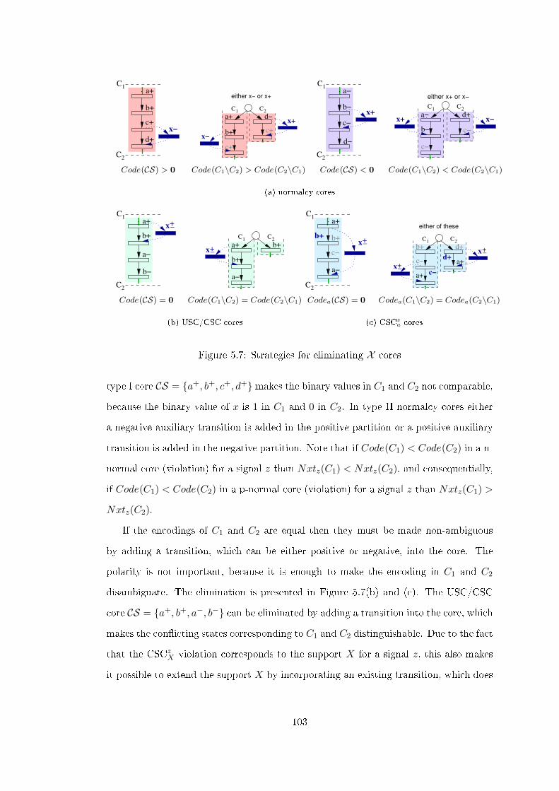
x−

C2

1C

b+

a+

d+

c+

C1

x−

C2

x+a+

b+

d−

c+

c+

either x− or x+

Code(CS) > 0 Code(C1\C2) > Code(C2\C1)

x+

1C

C2

d−

a−

c−

b− C1 C2

x+ x−a−

b−

d+

c−

c−

either x+ or x−

Code(CS) < 0 Code(C1\C2) < Code(C2\C1)

(a) normalcy cores

x+_1C

C2

b−

a−

a+

b+ C1 C2

+_ a+

a−

b+

b+x

Code(CS) = 0 Code(C1\C2) = Code(C2\C1)

(b) USC/CSC cores

1C

C2

+_x

a+

b+b+

c−

a−

C1 C2

+_

+_x a+

d+d+

c−

x

a+

c−

b+

either of these

Codea(CS) = 0 Codea(C1\C2) = Codea(C2\C1)

(c) CSCza cores

Figure 5.7: Strategies for eliminating X cores

type I core CS = {a+, b+, c+, d+} makes the binary values in C1 and C2 not comparable,because the binary value of x is 1 in C1 and 0 in C2. In type II normalcy cores eithera negative auxiliary transition is added in the positive partition or a positive auxiliarytransition is added in the negative partition. Note that if Code(C1) < Code(C2) in a n-normal core (violation) for a signal z than Nxtz(C1) < Nxtz(C2), and consequentially,if Code(C1) < Code(C2) in a p-normal core (violation) for a signal z than Nxtz(C1) >

Nxtz(C2).If the encodings of C1 and C2 are equal then they must be made non-ambiguous

by adding a transition, which can be either positive or negative, into the core. Thepolarity is not important, because it is enough to make the encoding in C1 and C2

disambiguate. The elimination is presented in Figure 5.7(b) and (c). The USC/CSCcore CS = {a+, b+, a−, b−} can be eliminated by adding a transition into the core, whichmakes the con�icting states corresponding to C1 and C2 distinguishable. Due to the factthat the CSCz

X violation corresponds to the support X for a signal z, this also makesit possible to extend the support X by incorporating an existing transition, which does

103

not correspond to X, in the core. For example the core CS = {a+, b+, c−, a−} can beeliminated by using a transition, e.g. b+, from CS to disambiguate the con�icting statesand take its signal into the support.

5.3.2 X core elimination by signal insertion

State coding con�icts can be e�ciently resolved by introducing �additional memory�to the system in the form of internal signals. Depending on X the con�icting statesare made either not comparable or disambiguated by the �additional memory�. Thisapproach requires behavioural equivalence of the speci�cation and a guarantee that thesignals are implemented without hazards, preserving speed independence [19]. In orderto resolve the con�icting states caused by X cores, auxiliary signals must be added tothe speci�cation. Two methods of insertion are described. First, single signal insertion isdescribed, which introduces one signal per targeted core. Secondly, dual signal insertionis presented which produces �ip �ops by inserting complementary signal pairs.

5.3.2.1 Single signal insertion

In order to resolve the con�icting states caused by an X core, an auxiliary signal auxis added to the speci�cation. The elimination of an X core is schematically illustratedin Figure 5.8. An X core can be eliminated by inserting a transition of aux, say aux+,somewhere in the core to ensure that it is no longer a con�ict set. To preserve theconsistency of the STG, the signal transition's counterpart aux− must also be added tothe speci�cation outside the core, in such a way that it is neither concurrent with, norin structural con�ict with aux+ (otherwise the STG becomes inconsistent). Anotherrestriction is that an inserted signal transition cannot trigger an input signal transition.The reason is that this would impose constraints on the environment which were notpresent in the original STG, making input signal �wait� for the newly inserted signal.A transition can be inserted either by splitting an existing transition, or by inserting atransition concurrent with an existing transition.

The elimination of X cores is illustrated by using typical cases in STG speci�cations.Figure 5.9 shows a case where two CSC cores are in sequence. They can be eliminated in

104

aux+

aux−

−coreX

Figure 5.8: X core elimination by signal insertion

a �one-hot� manner. Each core is eliminated by one signal transition, and its complementis inserted outside the core, preferably into non-adjacent one. The union of two adjacentcores is usually a con�ict set, which will not be destroyed if both the transition and itscounterpart are inserted into it. This case is shown in Figure 5.9(a), where the risingtransition of a newly added signal, csc+0 , is inserted in the �rst core and its counterpartis inserted in the second core. This results in another core formed by the union ofthose cores including the newly inserted signal. However, this core can be eliminatedby another internal signal. The insertion of a transition into the �rst core and itscounterpart outside the core, but not in the adjacent core, is shown in Figure 5.9(b).The second core can be eliminated in the same way. Both approaches use two additionalinternal signals to eliminate the cores.

csc0+

csc0− csc

0−

csc0+

a0−

a1−

a1+

c0−

c1+

c0+

b0−

b1+

b0+

c1−

b1−

a0+

a0−

a1−

a1+

c0−

c1+

c0+

b0−

b1+

b0+

c1−

b1−

a0+

(a)

csc0− csc

0−

csc0+ csc

0+

a0−

a1−

a1+

c0−

c1+

c0+

b0−

b1+

b0+

c1−

b1−

a0+

a0−

a1−

a1+

c0−

c1+

c0+

b0−

b1+

b0+

c1−

b1−

a0+

(b)

inputs: a0 , b0 , c0 ; outputs: a1 , b1 , c1 ; internal: csc0

Figure 5.9: Example: elimination of CSC cores in sequence

The case where a CSC core is located in a concurrent part is shown in Figure

105

5.10(a). It can be also tackled in a one-hot way. A signal transition, say csc+, isinserted somewhere in the core and its counterpart outside the core. Note that in orderto preserve the consistency the transition's counterpart cannot be inserted into theconcurrent part, but it can be inserted before the fork transition or after the join. Inthis example, the counterpart transition csc− can be only inserted after b+, splittingb+. Inserting csc− before b+ would not eliminate the core but it would extend the coreby the csc signal. The same happens if csc− is inserted after a+. The insertion beforea+ is not possible because a+ corresponds to an input signal.

b−

b+

a+

a−

csc+

c+

d−

c−

d+

csc−

split

split

inputs: a, d

outputs: b, c

internal: csc

(c)

a+

c+

b+

d+

e+

a−

c−

b−a+

e−

c+

d−

csc−

csc+

inputs: a, b

outputs: c, d , e

internal: csc

(c)

Figure 5.10: Example: elimination of CSC cores in concurrent parts

X cores partly located in a concurrent part as the one shown in Figure 5.10(b),where X is CSC, can be handled in the same way. If a transition is inserted in a corein a concurrent part then its counterpart cannot be inserted concurrent to it. However,if a transition is inserted in a core in a sequential part then its counterpart is insertedsomewhere outside the core as illustrated in Figure 5.10(b).

The elimination of X cores which are located in branches which are in structuralcon�ict (due to choice) are also done in a one-hot way. First consider the case where aCSC core is completely located in one con�icting branch as shown in Figure 5.11(a). Inorder to preserve consistency, the transition inserted outside the core cannot be insertedin the con�icting branch. It must be inserted in the same branch as the core, between

106

csc+

a−

r−

a+

r+

s−

a−

c+

a+OR

d+

s+

c+

d−

csc−

c−

merge

split

inputs: a, c, s

outputs: d , r

internal: csc

(a)

a−

b−

e−

d−

e+

a−

c+OR

b+

d−

a+merge

d+

c−

csc−

split csc+

csc−

inputs: a, c

outputs: b, d , e

internal: csc

(b)

b+/2a+

f−

b+/1

e+

d+

b−/2

a−

e−

f+

b−/1

c−

merge

csc−

split

csc+

d−

c+

csc−

inputs: a, b, c

outputs: d , e, f

internal: csc

(c)

Figure 5.11: Example: elimination of CSC cores in choice branches

the choice and the merge point, as shown in Figure 5.11(a). Alternatively, a transitioncan be inserted in each branch and its counterpart before the choice point or after themerge point, or vice versa, as demonstrated in Figure 5.11(b). A core can be partlylocated in a con�icting branch or in more than one con�icting branch as shown in Figure5.11(b) and (c), respectively. Those cases can be solved in the same way, as long as thecounterpart to the additional transition in the X core is inserted in such a way that itdoes not validate the consistency property.

Figure 5.12 summarises the insertion possibilities in typical cases in STG speci�ca-tions. X cores in sequence can be eliminated in a one-hot manner as depicted in Figure5.12(a). Each X core is eliminated by one signal transition, and its complement is in-serted outside the X core, preferably into non-adjacent one. An STG that has a X corein one of the concurrent branches and in one of the branches which are in structuralcon�ict, respectively, can also be tackled in a one-hot way, as shown in Figure 5.12(b)and (c), respectively. In order to preserve the consistency the transition's counterpartcannot be inserted into the concurrent branch or into the con�icting branch. Obviously,the described cases do not cover all possible situations or all possible insertions (e.g.

107

aux−

aux−

aux+

aux−

(a) sequential

fork

join

aux−

aux−

aux−

aux−aux+

aux−

(b) concurrent

choice

mergemerge

aux−

aux−

aux−

aux+

aux−

aux−

(c) structural con�ict

Figure 5.12: Strategies for X core elimination

a signal transition can sometimes be inserted before the choice point or after a mergepoint and its counterparts inserted into each branch, etc.), but they give an idea howthe X cores can be eliminated.

5.3.2.2 Dual signal insertion (�ip �op insertion)

The insertion of pairs of complementary signals [ff±0 , ff∓1 ] in the STG implicitly adds a

pair of negative gates to the circuit and creates a �ip �op, which makes one part of theSTG unordered with the other. This type of insertion gives the designer opportunitiesfor potential improvements to the circuit. The insertion of pairs of complementarysignals is illustrated in Figure 5.13. The insertion of two auxiliary signal transitionsff0 and ff1, such that ff±0 is a direct predecessor of ff∓1 is denoted by ff±0 � ff∓1 .The transformation [ff+

0 , ff−1 ] denotes the insertion of ff+

0 � ff−1 and ff+1 � ff−0 ,

and similarly the transformation [ff−0 , ff+1 ] denotes the insertion of ff−0 � ff+

1 andff−1 � ff+

0 . The former is realised by a �ip �op constructed from two NAND gatesand the latter is realised by a �ip �op constructed from two NOR gates. The �ip �opinsertion is classi�ed as follows:

Simple �ip �op insertion illustrated in Figure 5.13(a) performs a transformation, e.g

108

trig −ff1

trig +ff1

trig +ff0

trig −ff0

ff −0

ff +1

ff −1

ff +0

ff +0

ff −1

ff +1

ff −0

ff1

ff0

trig −ff1

trig −ff0

trig +ff0

ff0trig +ff1

ff0

... ...targettarget

target target

set ff0

reset ff0

reset ff

set ff0

0

(a) simple

trig −ff1

trig +ff1

trig +ff0

trig −ff0

trig +ff1

trig −ff1

trig −ff0

trig +ff0

ff +0

ff −1

ff +1

ff −0

ff −0

ff +1

ff −1

ff +0

trig −ff0

trig +ff0

ff1

ff0

ff1

ff0trig +

ff0trig −

ff0

trig −ff1

trig +ff1 trig +

ff1

trig −ff1

... ...

targettarget

target target

set ff0

reset ff

reset ff

set ff0 0

0

(b) complex

Figure 5.13: Strategy for �ip �op insertion

[ff+0 , ff

−1 ], where ff−1 and ff−0 each have only one direct predecessor, ff+

0 andff+

1 , respectively. The signal ff0 is set by at least the trigger of ff+0 and is reset

by at least the trigger of ff−0 . Note that contextual signals may be involved forwhich additional logic is required at the inputs of the �ip �op.

Complex �ip �op insertion illustrated in Figure 5.13(b) works in a similar way, butif the transformation [ff+

0 , ff−1 ] is inserted ff−1 and ff−0 have each at least one

direct predecessor. If both have only one direct predecessor than the insertion cor-responds to a simple �ip �op insertion. Otherwise, the extra triggers contributeto additional logic at the criss-cross inputs of the �ip �op. Note that contextualsignal may also contribute to the additional logic. In Figure 5.13(b) in the trans-formation [ff+

0 , ff−1 ] both ff−1 and ff−0 have two triggers, ff−1 is triggered by ff+

0

and trig+ff1

, and ff−0 is triggered by ff+1 and trig+

ff0, which control the criss-cross

inputs.

In both cases a �ip �op is realised. Its complexity depends on the triggers of ff0 andff1. Due to the nature of �ip �ops, and to avoid hazards, the set and reset functions

109

must be non-overlapping, e.g. if it is constructed from two NAND gates and bothinputs go to '0' then both outputs go to '1', violating the fact that both outputs mustbe complements of each other.

c−

b−a+

e−

csc+

d−

c+

csc−

a+

b+

d+

e+

a−

c+

(a) single signal insertion

ff +0ff −1

ff −0

ff +1

c−

a+

e−d−

b−

c+

a+

b+

d+

e+

a−

c+

(b) dual signal insertion

b

csc

cde

a

(c) implementation for (a)

ff1

ff0

e

d

c

b

a

(d) implementation for (b)

inputs: a, b; outputs: c, d , e; internal: csc,ff0 ,ff1

Figure 5.14: Example: �ip �op insertion

Consider the example in Figure 5.14, where single and dual signal insertion areused to eliminate the CSC core. The former is depicted in Figure 5.14(a), showing thesequential insertion of signal csc; csc− is inserted in the core →od− and csc+ is insertedoutside the core →oc+. The resulting implementation is shown in Figure 5.14(c).

The dual signal insertion is presented in Figure 5.14(b), where [ff+0 , ff

−1 ] are inserted

realising a NAND �ip �op; ff+0 � ff−1 is inserted in the core →od− and ff+

1 � ff−0 isinserted outside the core →oc+, such that •(•ff−0 ) = {a+, ff+

1 }. According to the ruleabove, this transformation should result in an complex �ip �op because ff−0 has morethan one predecessor. However, due to the fact that a− is a trigger of ff+

0 , the triggersof the signal ff0 are a and ff1. Thus the �ip �op does not need additional control logic.It is set by a and reset by b. The implementation of this transformation is depicted inFigure 5.14(d). Note that the �ip �op insertion corresponds to inserting the auxiliarysignal ff0 �rst (ff+

0 →od− and ff−0 →oc+) followed by ff1 (ff−1 →od− and ff+1 b−o→).

110

The dual signal insertion introduces a delay of two units whereas a single signalinsertion introduces a delay of only one unit (but this one unit is typically a complexgate, which is implemented by two negative gates.) For example, d− is delayed by ff+

0

and ff−1 in the former case and d− is delayed by csc− in the latter. However, due tothe simplicity of the gates in the implementation with �ip �ops, the latency of bothimplementations is similar. Generally, the dual signal insertion can be used for thedecomposition of complex gates.

5.3.3 X core elimination by concurrency reduction

Concurrency reduction involves removing some of the reachable states of the STG, andcan therefore be used for the resolution of encoding con�icts. The elimination of X coresby concurrency reduction involves the introduction of additional ordering constraints,which �x some order of execution. In an STG, a fork transition de�nes the startingpoint of concurrency, and a join transition de�nes the end point. Existing signals canbe used to resolve the con�icting states in an X core by delaying the starting point orbringing forward the end point of concurrency. Depending on X the con�icting statesare either made not comparable or unambiguous. If there is an event concurrent to anX core, and a starting or end point of concurrency in the core, then this event can beforced into the core by an additional ordering constraint. Thus, the core is eliminated,unless the core corresponds to a normalcy violation and the polarity of the transitionused does not eliminate the core.

Two kinds of concurrency reduction transformations for X core eliminations aredescribed below.

Forward concurrency reduction illustrated in Figure 5.15(a) performs the concur-rency reduction h(EU )

n99K h(g) in the STG, where EU is a maximal (w.r.t⊂) set

of events outside the X core in structural con�ict with each other, and concurrentto g, an event in the X core. It is assumed that e is in the X core, either e ≺ g

or e ‖ g, and for exactly one event f ∈ EU , e ≺ f .

Backward concurrency reduction illustrated in Figure 5.15(b) works in a similar

111

core

f

g

e

core

d

fp

e

g

(a) forward

core

f

g

e core

p

d

f

e

g

(b) backward

Figure 5.15: X core elimination by concurrency reduction

way, but the concurrency reduction h(EU )n

99K h(f) is performed. It is assumedthat e is in the X core, f is an event outside the X core such that f ≺ e, EU isa maximal (w.r.t⊂) set of events which are in structural con�ict with each otherand concurrent to f , such that exactly one event g ∈ EU is in the X core, andeither g ≺ e or g ‖ e.

In both cases the X core is eliminated by additional ordering constraints �dragging� finto the core. Note that the polarity of the transition corresponding to f is important forthe elimination of a p-normal and an n-normal core (see section 5.3.1). The eliminationof such a core requires the polarity of h(f) to be opposite to the one in the core, i.e. ifthe targeted core partition is negative than h(f) must be positive in order to eliminatethe core and vice versa.

These two rules are illustrated by the examples in Figure 5.16 and 5.17 where theyare applied to CSC cores of types I and II . In Figure 5.16(a) instances of b+ and a−

are concurrent to the CSC core. The forward concurrency reduction b+ 99K e− can beapplied, because b+ succeeds e+ and e− succeeds e+. This �drags� b+ into the core,destroying it. This means that the con�icts corresponding to the core are disambiguatedby the value of the signal b. Note that f is an input and thus cannot be delayed, and sothe concurrency reductions b+ 99K f+ and b+ 99K f− would be invalid. The backward

112

f−

e−

e+

f+

b+

a−

d+

a+

c−

d−

c+b−

inputs:b, c, f ;outputs:a, d , e

forward reduction: b+ 99K e−

backward reductions: e+ 99K a−; f+ 99K a−

2p

1p p’

c+

c−

a+

e−

d−

e+

d+

c−

a−

c+

b−

b+

inputs: a, b;outputs: c, d , e

backward reduction: {a+, b+} 99K d+

(a) (b)

Figure 5.16: Elimination of type I CSC cores

concurrency reductions e+ 99K a− and f+ 99K a− can also be applied to eliminate thecon�ict core, because a− precedes e−, and both e+ and f+ are in the core and precedee−. Either of these reductions �drags� a− into the core, destroying it. The con�ictscaused by the core are disambiguated by the signal a.

In Figure 5.16(b), d+ is concurrent with events in the core and precedes c+, an eventin the core. The only event in the core which precedes or is concurrent to c+ is a+.However, a+ 99K d+ is an invalid transformation, which introduces a deadlock. Theconcurrency reduction {a+, b+} 99K d+ is used instead, since b+#a+ and b+ ‖ d+.

Figure 5.17 shows the elimination of type II CSC cores. A forward concurrencyreduction is illustrated in Figure 5.17(a). An instance of d+ is concurrent to the coreand succeeds a+, an event in the core, and can therefore be used for a forward reduction.The only possible concurrency reduction is d+ 99K a−, since b+and e+ is an input andthus cannot be delayed.

The backward concurrency reduction technique is illustrated in Figure 5.17(b),where d+ is concurrent to a+ and e+ in the core and precedes b+ in the core. The only

113

e8

e6

e3

e1

e7

e2

e4

e9

e11

e10

e0

e5

c+

c−

b−/1

b−

d−

d+

e+

a−

b+

a+

e− b+/1

inputs:b, e;outputs:a, c, d

forward reduction: d+ 99K a−

p2

p1

b+/1

b+ e+

c−

b−/1

a+

a−

e−

c+

d+

f+

d−

b−f−

p’p’’

inputs: a, b, f ;outputs: c, d , e

backward reductions:{a+, c+} 99K d+; {c+, e+} 99K d+

(a) (b)

Figure 5.17: Elimination of type II CSC cores

events in the core which either precede or are concurrent with b+ are a+ and e+, andeither of these can be used to eliminate the core. However, both reductions a+ 99K d+

and e+ 99K d+ are invalid, since they introduce deadlocks, and are not allowed bythe backward concurrency reduction. Thus c+ should be involved, yielding the follow-ing two backward concurrency reductions eliminating the core: {a+, c+} 99K d+ and{c+, e+} 99K d+. Note that the reductions {a+, b+/1} 99K d+ and {b+/1, e+} 99K d+

do not eliminate the core, because d+ is `dragged' into both branches of the core, andso the net sum of signals in these two branches remains equal. (The backward concur-rency reduction rule does not allow use of these two transformations, since only oneevent from the set EU is allowed in the core.)

5.3.4 Resolution constraints

It is often the case that X cores overlap. In order to minimise the number of transforma-tions (either concurrency reduction or signal insertion), and thus the area and latencyof the circuit, it is advantageous to transform a speci�cation in such a way that as manycores as possible are eliminated. That is, a transformation should be performed at the

114

intersection of several cores whenever possible.To assist the designer in exploiting X core overlaps, another key feature of this

method, viz. the height map showing the quantitative distribution of the X cores, isemployed in the visualisation process. Figure 5.18 schematically illustrates the relation-ship between the representation of X cores and the height map. The events located inX cores are highlighted by shades of colours. The shade depends on the altitude of anevent, i.e. on the number of cores to which it belongs. (The analogy with a topograph-ical map showing altitude may be helpful here.) The greater the altitude, the darkerthe shade. �Peaks� with the highest altitude are good candidates for transformation,since they correspond to the intersection of maximum number of cores. In Figure 5.18the area labelled �A3� is the area of highest density where all three cores intersect.

A1A2A3

Height mapCore map

123

Figure 5.18: Visualisation of encoding con�icts

In Figure 5.19(a) there are �ve CSC cores altogether and all of them overlap. Peakswith the highest altitude are labelled �A5�. It is possible to eliminate them by addingjust one new signal: one of its transitions should be inserted into the intersection ofthese cores, and its counterpart into the remaining part as depicted in Figure 5.19. Inthe second phase of the signal insertion the altitudes are made negative in the heightmap by using the information from the height map in phase one. Note that the coreswhich are not targeted are not made negative. Additionally, in the height map thoseareas where a transition cannot be inserted are faded out preserving consistency. In theexample in Figure 5.19 no events are in structural con�ict with and concurrent with thetransition inserted in phase one, thus no events are faded out.

The example in Figure 5.20 shows a n-normalcy violation for signal b. This isre�ected in the equation for b, which is presented in Figure 5.20(b), where b is n-normalw.r.t a and c and p-normal w.r.t d. The violation is caused by two cores, CS1 and CS2

115

54321

x+

c+

x−

c−

x+

b−

y+

y−’

y+ x−

a−

y−

x+

c+

x−

c−

x+

y−

y−

y+ x−

a−

y+’

b−

e9 e8

e7

e6

e5

e1 e2

e3 e4

e10

e11 e12

e13

e14

e9 e8

e7

e6

e5

e1 e2

e4

e11 e12

e13

e14

e10

e3

height map

b+ a+A0

A5

A3

A1

1,2,4

1,2,3,4,5

1,3,51,3,4

1

1

1,3,4

1

b+ a+

core map

split x−

(a) phase one

x+

c+

c−

x+

b−

y−

y+

y−

y+ x−

a−

x−

b+ a+

csc+

height map

A−5

A0

A−1

A−3

insertingconcurrently

csc−

e3 e4

e6e7

e8

e9

e11

e12 e13

e15

e1 e2

e5

e10

e14

(b) phase two

inputs: a, b, c; outputs: x , y ; internal: csc

Figure 5.19: Intersection of CSC cores

which overlap. Events labeled �A2� in the height map belong to the highest peaks andare good candidates for signal insertion. In phase one, a negative auxiliary transitionn− is inserted into the peak, because the encoding in CS1 and CS2 is positive. The onlyway to insert n− into the peak is before d+. Note that the signal c is an input signal,and therefore cannot be delayed by an insertion. In phase two n+ is inserted outsidethe cores, as indicated on the updated height map. The events with the altitude �A0�indicate that if n+ is inserted in the highest peak, then the two targeted cores CS1 andCS2 are eliminated. This results in a normal STG, which can be implemented withmonotonic gates as shown in Figure 5.20(c).

Using the height map representation, the designer can select areas for transformationand obtain a local, more detailed description of the overlapping cores with the selection.When an appropriate core cluster is chosen, the designer can decide how to perform thetransformation optimally, taking into account the design constraints and knowledge ofthe system being developed.

116

e4

e2

e5

e1

e0

e6

e7

e3

e4

e2

e5

e1

e0

e6

e7

e3

21

A2A1A0

e4

e2

e5

e1

e0

e6

e7

e3

a−

a+

b−

c+

c−

b+

d−

d+ split

a−

a+

d−

d+

b+

c−

c+

b−

core mapheight map

phase one

height map

phase two

A0

A−2A−1

a−

a+

d−

d+

b+

c−

c+

b−

splitn+

n−

(a) resolution process

b = c · d + a

d = a · d + c

(b) non-monotonic implementation

b = c · n + a

d = n

n = c · d + a

(c) monotonic implementation

inputs: a, c; outputs: b, d ; internal: n

Figure 5.20: N-normalcy violation for signal b

5.4 Resolution process

The advantage of using X cores is that only those parts of STGs which cause encod-ing con�icts, rather than the complete list of X con�icts, are considered. Since thenumber of X cores is usually much smaller than the number of encoding con�icts,this approach avoids the analysis of large amounts of information. Resolving encodingcon�icts requires the elimination of cores by introducing either additional signals orcausal constraints into the STG. A manual resolution and an automated resolution arepresented. The former uses several interactive steps aimed at helping the designer toobtain a customised solution, and the latter uses heuristics for transformation whichare based on X cores and their superpositions. However, in order to obtain an optimalsolution, a semi-automated resolution process can be employed, where several precom-puted solutions are suggested and the designer can choose the one which suits the designconstraints best.

117

5.4.1 Manual resolution

The overview of the manual resolution process of encoding con�icts is illustrated inFigure 5.21. Given an STG, a �nite complete pre�x of its unfolding is constructed, andthe X cores are computed. If there are none, the process stops. Otherwise, the heightmap is shown for the designer to choose a set of overlapping cores in order to performa transformation. The transformation, either concurrency reduction or signal insertion,is chosen by the designer. The former can only be applied if concurrency exists andeither starts or ends in the selected core overlaps, and if it is possible to either delaythe starting point or bring forward the end point. If this is the case, a causal constraintis inserted and transferred to the STG, and the process is repeated.

insert causalconstraint

the STGconstraint to

transfer

STG

unfold andcompute cores

conflictsexist

show theheight map

select a peak

show corescomprisingthe peak

formationinsert newtransition

select a peak

the peakcomprisingshow cores

insert thetransition’s

complement

transfer

the STG

show theheight map

update

yesnostop

signal insertion

phase 1

phase 2

signal to

concurrency reduction

choose trans−

Figure 5.21: The resolution process of encoding con�icts

An auxiliary signal can be inserted into the speci�cation in two phases. In phase onea signal transition is inserted and in phase two its counterpart is inserted eliminatingthe selected cores. The inserted signal is then transferred to the STG, and the process

118

is repeated. Depending on the number of X cores, the resolution process may involveseveral cycles.

After the completion of phase one, the height map is updated. The altitudes of theevents in the core cluster where the new signal transition has been inserted are madenegative, to inform the designer that if the counterpart transition is inserted there,some of the cores in the cluster will reappear. Moreover, in order to ensure that theinsertion of the counterpart transition preserves consistency, the areas where it cannotbe inserted (in particular, the events concurrent with or in structural con�ict with thistransition) are faded out.

5.4.1.1 Transformation condition

Next, conditions for transformation are presented, so that suitable transformations areselected. These conditions aim to minimise the circuit's latency and complexity. Trans-formations can introduce delays to non-input signal transitions, e.g. transition splittingdelays at least one transition, whereas concurrency reduction may introduce a delaydepending on the inserted causal constraint. Transformations such as concurrency re-duction and concurrent signal transition insertion can introduce transitions which have alarge number of incoming and outgoing arcs, respectively. This results in a circuit wheresome gates can be complex, i.e. have a large fan-in/fan-out. Modern asynchronous cir-cuits are usually built of CMOS gates, with ASIC gate array libraries which consist ofa restricted number of rather simple gates depending on four, or fewer variables. Thismeans that the number of incoming and outgoing arcs of a transition should not exceedfour. Clearly, the transformation which produces a minimal fan-in/fan-out should bechosen over the one with relatively high fan-in/fan-out.

The polarity of the introduced transitions can have an e�ect on the complexity ofa circuit by introducing additional input inverters in the case of USC/CSC resolution.Those inverters are often assumed to have zero delay for the circuit to function correctly.If they are viewed as ordinary gates with delays, there could be a situation where suchan inverter might switch concurrently with the gate it is connected to. Such a situationmay lead to glitches. In the case of normalcy resolution, much more care is required

119

during the transformation not to destroy the existing normalcy. This is done in such away that the polarity should not introduce di�erent and/or contradictory triggers forexisting normal signals.

The polarity for USC/CSC resolution is not crucial for the elimination of suchencoding con�icts. Thus, the polarity could be chosen to preserve and/or to improvenormalcy by means of triggers, e.g using consistent and non-contradictory triggers. Thiswould ensure that the triggers, which generally arrive at the latest point, do not needto be inverted and thus reducing the risk of hazards. Additionally, it is essential thattransitions in an STG alternate up and down to increase the use of negative gates. Atransformation which generates an alternating polarity can reduce the complexity. Thelatter can also be applied to normalcy resolution.

The above conditions are summarised as follows, and should be applied to select asuitable transformation:

1. minimum delay

2. minimum fan-in/fan-out

3. consistent polarity of triggers

4. non-contradictory triggers

5. alternating polarity of transitions

Note, that conditions 3 and 4 are necessary for normalcy resolution, where e.g. theintroduction of inconsistent triggers would violate the normalcy property.

5.4.1.2 Resolution examples

In order to demonstrate the resolution of encoding con�icts, two examples are presentedshowing CSC and normalcy resolution.

CSC con�ict resolution Figure 5.22 illustrates the transformation process. Theheight map in Figure 5.22(a) shows the distribution of CSC cores. The events labeled�A3� belong to the highest peak, corresponding to three overlapping cores depicted

120

e2

e3

e4

e5

e6

e7

e8

e9

e10

e0 e

1 A1A2A3

e5

y−

a−

x/1−

z−

x/1+

b−

x−

b+

x+

z+a+

y+

(a) height map

e2

e3

e4

e6

e7

e8

e9

e0 e

1

e11

e10

e5

y−

a−

x/1−

z−

x/1+

b−

x−

b+

x+

z+a+1

2

3

constraintcausal

23

1

y+

(b) concurrency reduction

e4

e6

e7

e8

e9

e11

e2

e3

e0 e

1

e5

e10

e4

e6

e7

e8

e9

e2

e3

e0 e

1 123

e5

e10

e11

a−

x/1−

z−

x/1+

b−

x−

b+

x+

z+a+

csc−

3

2

1

y+

y−

split

a−

x/1−

z−

x/1+

b−

x−

y−

b+

x+

z+a+

csc−

csc+

3

y+

split

phase 2: height mapphase 1: cores

A0A−1A−2A−3

(c) signal insertion

inputs: a, b; outputs: x , y , z ; internal: csc

Figure 5.22: CSC con�ict resolution

in Figure 5.22(b) and (c). The designer can choose either concurrency reduction orsignal insertion. A forward concurrency reduction is possible because e5 is concurrentwith the events in the highest peak and e5 succeeds e3, which belongs to the highestpeak. The causal constraint h(e5) 99K h(e4) is inserted and this eliminates the cores(see Figure 5.22(b)). Note the order of execution: e5 is executed before e4 and thearc between b+ and x− becomes redundant. Thus the signal y, which corresponds toe5, is used to disambiguate the con�icting states corresponding to the cores. However,this transformation introduces a delay, x− is delayed by y+. Due to the fact that thepolarities of the triggers of the signal x have been contradictory, the transformationdoes not e�ect this, the positive trigger of x− is replaced by another positive trigger.In order to make the triggers of x non-contradictory the triggers of either x+ and x−/1or x− and x+/1 must be modi�ed.

Signal insertion is shown in Figure 5.22(c). In phase one an auxiliary signal transitioncsc− is inserted somewhere into the peak, e.g. csc− can be inserted h(e3)o→. Afterupdating the height map the second phase can be performed. In order to eliminate allthree cores csc+ must be inserted in the highest peak, which corresponds to events with

121

the altitude �A0�, e.g. csc+ is inserted →oe11. The signal csc is used to disambiguatethe state coding con�icts. The transformation is transferred to the STG resulting ina con�ict-free STG. The transformation introduces the following delays: the insertionin phase one delays x− and y+, and the insertion in phase two delays y−. The newinserted signal csc and the signal y have non-contradictory triggers.

Normalcy con�ict resolution The example shown in Figure 5.23 has a CSC con�ictand a p-normalcy violation for signals c and d. The corresponding cores CS1 to CS4 areillustrated in Figure 5.23(a) to (c). It is necessary to eliminate CS1, which correspondsto CSC con�icts, to make the speci�cation implementable. In order to obtain monotonicfunctions the remaining three cores must also be eliminated. The CSC core CS1 canbe eliminated by applying a forward concurrency reduction h(e5) 99K h(e7) as shownin Figure 5.23(d). This transformation will also eliminate CS3 and CS4, because d+

will make the con�icting states corresponding to CS3 and CS4 not comparable. Notethat the encoding in CS3 only di�ers by the value of signal e and the encoding in CS4

only di�ers by the value of c and e. Therefore, adding a positive transition into the leftpartition of CS3 and CS4 results in the elimination of these cores. However, CS2 stillremains. This is re�ected in the equation for signal c (see Figure 5.23(d) step 1), wherec is neither p-normal nor n-normal. It is p-normal w.r.t b and n-normal w.r.t. a and d.In order to eliminate CS2 a negative transition must be added into the left partition,say n−0 , and its counterpart n+

0 must be added in the same branch outside the core topreserve consistency. The only way to insert n+

0 is →od−, however n+0 is positive and

would make d not normal, i.e. n+0 would trigger d− (this would suggest that d is n-

normal), but d+ is triggered by a+(this would suggest that d is p-normal). To overcomethis n−0 could be inserted →od+ making the triggers of d n-normal as shown in Figure5.23(d) in step 2. This solution satis�es the normalcy property, which is re�ected inthe equations. However, n-normal cores for d could appear after inserting n0. Thistransformation would delay two transitions, as d+ and d− are delayed by n−0 and n+

0 ,respectively. Note that the concurrency reduction does not introduce any delay; d+ isexecuted concurrently with b+.

122

e8

e6

e3

e1

e7

e2

e4

e9

e11

e10

e0

e5

CS1

c+

c−

b−/1

b−

d−

d+

e+

a−

b+

a+

e− b+/1

(a) CSC con�ict

e8

e6

e3

e1

e7

e2

e4

e9

e11

e10

e0

e5

CS2

c+

c−

b−/1

b−

d−

d+

e−

a+

b+

a−

e+

b+/1

(b) p-normalcy violation forsignal c

e8

e6

e3

e1

e7

e2

e4

e9

e11

e10

e0

e5

CS3 CS4

c−

b−/1

b−

d−

e+

e−

a+

a−

b+

b+/1

d+

c+

(c) p-normalcy violation forsignal d

e8

e6

e3

e1

e7

e2

e4

e9

e11

e10

e0

e5

CS3CS1

CS4

c−

b−/1

b−

d−

e−

a+

a−

b+

b+/1

d+

c+

e+

a = e · (d + b)

c = b · d · ad = b · d + a

step 1

0n −

0n +

e8

e6

e3

e1

e7

e2

e4

e9

e11

e10

e0

CS2

e5

c−

b−/1

b−

d−

e−

a+

a−

b+

b+/1

c+

e+

d+

a = e · (d + b)

c = n0 · b · ed = n0

n0 = a · (d + b)

step 2

e8

e6

e3

e1

e2

e4

e9

e11

e10

e0

e5

CS3CS1

e7

n +0

n −0

CS4

c−

b−/1

b−

d−

e−

a+

a−

b+

b+/1

d+

c+

e+

a = e · n0

c = b · n0 · ad = n0 + a

n0 = b · (n0 + a)

step 1

e9

e6

e3

e1

e10

e0

e5

CS’1

e2

e4

n −0e

13

e14

e11

e8

e6 n +0

n +1

n −1

CS’2

c−

b−/1

b+/1

d+

c+

e+

a+

b+

b−

d−

a−

e−

a = e · n0

c = n1 · e · bd = n0 + a

n0 = n1

n1 = a·n0 + b

step 2

(d) �rst transformation (e) second transformation

inputs: b, e; outputs: a, c, d ; internal: n0 ,n1

Figure 5.23: Normalcy con�ict resolution

123

Alternatively, the CSC core CS1 can be eliminated by a signal insertion, say n0,which can be used to eliminate either the normalcy violation for c or the normalcyviolation for d. Depending on the polarity of the transition, the insertion of one ofthese can also eliminate a normalcy violation. A positive transition of n0 eliminatesCS3 and CS4, and a negative transition eliminates CS2. The former is illustrated inFigure 5.23(e) in step 1. From the equation for d it can be seen that it is p-normal.However, c is still not normal. An additional signal insertion is needed to eliminate thenew p-normal cores C ′

1 and C ′2 (see Figure 5.23(e) in step 2), which arise after the �rst

step of the resolution process. These cores can be eliminated by inserting a negativeauxiliary transition n−1 into the intersection of the cores and its counterpart outside thecore, in such a way that the existing normalcy is not destroyed, e.g. without changingthe polarity of triggers of the normal non-input signals. Inserting n−1 before a+ wouldnot violate n-normalcy for a, since a+ already has a negative trigger e−. However, it isnot possible to insert n+

1 in the same branch without destroying some normalcy, e.g. ifn+

1 is inserted before n−0 than n0 would have contradictory triggers, positive trigger forboth n+

0 and n−0 . The transition n−1 can be inserted →on+0 and its counterpart →on−0 .

Based on their triggers this would make n0 and n1 n-normal. This transformation ispresented in Figure 5.23(e) in step 2 with results in a monotonic implementation. Thistransformation delays a− by n+

0 and n−1 and it also delays d− by n−0 and n+1 .

0n −

0n +

e9

e7

e3

e1

e8

e2

e6

e0

e4

e5

e10

e11

e12

e13

c−

b−/1

d−

c+

d+ b+

a+

e− b+/1

a−

e+

b−

(a) unfolding pre�x

a = e · (d + b)

c = n0 · b · ed = n0

n0 = a · (d + b)

(b) equation beforedecomposition

a = e · n1

c = n0 · b · ed = n0

n0 = a · n1

n1 = d · b

(c) equation afterdecomposition

Figure 5.24: Logic decomposition (d+ b): signal insertion n+1 →oa− and n−1 →on+

0

In the equations in Figure 5.23(d) in step 2 (also shown in Figure 5.24(b)) the term

124

(d + b) calls for a possible decomposition. A new signal n1 can be inserted such thatn1 = d + b, which is then used as a new signal in the support for a and n0. Such atransformation would contribute to the derivation of simpler equations. However, caremust be taken not to increase the complexity of other functions.

In the equation a = e · (d + b) a+ is triggered by e− and a− is triggered by d+

and b+, and in the equation n0 = a · (d+ b) n+0 is triggered by b− and n−0 is triggered

by a+. In order to decompose the term (d + b) by the new signal n1, n1 should be inthe support of n0 and a. Thus, the triggers of a− and n+

0 should be replaced by thetransition of n1. Note that a signal's triggers are guaranteed to be in the support ofthis signal. To retain normalcy n+

1 is inserted→oa−. The result is that a is triggered byn1 and e, and n1 is triggered by b and d . Furthermore, the n-normality of the triggersof a is maintained. The counterpart transition n−1 is inserted →on+

0 . The result is thatb−, the trigger of n+

0 , is replaced by n+0 making a and n1 the triggers of n0, and also

maintaining the n-normalcy of the triggers of n0. Note also that the newly insertedsignal n1 has p-normal triggers, and its triggers are also maintained, i.e. b is already atrigger for n+

1 . The equations of the resulting STG are shown in Figure 5.24(c), wherelogic n1 = d · b is shared by a and n0.

5.4.2 Automated resolution

In the automated resolution process heuristics for transformations (either signal inser-tion or concurrency reduction) are employed, based on the X cores, their suppositionsand insertion constraints. Also, a heuristic cost function (see section 5.4.3) is appliedto select the best transformation for the resolution of con�icts. It takes into account:(i) the delay caused by the applied transformation; (ii) the estimated increase in thecomplexity of the logic and (iii) the number of cores eliminated by the transformation.

The resolution process involves �nding an appropriate transformation (either concur-rency reduction or signal insertion) for the elimination of X cores in the STG unfoldingpre�x. An overview is illustrated in Figure. 5.25. The following steps are used to resolvethe encoding con�icts con�icts:

1. Construct an STG unfolding pre�x.

125

d−

c+

a+

csc+

d−

c+

a+

e+

b−

c+f−

d−

c+

a+

e+

b−

c+f−

e+

b−

c+f−

extract compute select

core 1

core 2

core 4

core 5

core 3

split

cores in unfolding prefix areas for transformation valid transformations "good" transformation

Figure 5.25: Overview: automated resolution process

2. Compute the cores and, if there are none, terminate.

3. Choose areas for transformation (the �highest peaks� in the height map corre-sponding to the overlap of the maximum number of cores are good candidates).

4. Compute valid transformations for the chosen areas and sort them according tothe cost function; if no valid transformation is possible then

� change the transformation areas by including the next highest peak and goto step 4;

� otherwise manual intervention by the designer is necessary; the progressmight still be possible if the designer relaxes some I/O constraints, usestiming assumptions.

5. Select the best, according to the cost function, transformation; if it is a signalinsertion then the location for insertion of the counterpart transition is also chosen.

6. Perform the best transformation and continue with step 1.

5.4.3 Cost function

A cost function was developed to select heuristically the best transformation at eachiteration of the encoding con�ict resolution process (either a concurrency reduction or asignal insertion). It is based on speci�cation (STG unfolding pre�x) level optimisationand is very approximate, but it is not computationally expensive. The cost function is

126

composed of three parts, taking into account the delay penalty in�icted by the transfor-mation, the estimated increase in the complexity of the logic, and the number of coreseliminated by the transformation:

cost = α1 ·∆ω + α2 ·∆logic + α3 ·∆core. (5.1)

The parameters α1,2,3 ≥ 0 are given by the designer and can be used to direct theheuristic search towards reducing the delay in�icted by the transformation (α1 is largecompared with α2 and α3) or the estimated complexity of logic (α2 and α3 are largecompared with α1).

The �rst part of the cost function estimates the delay caused by a transformation.A delay model where each transition of the STG is assigned an individual delay isconsidered, e.g. input signals usually take longer to complete than non-input ones,because they often denote the end of a certain computation in the environment. Thisdelay model is similar to that in [14, 18]. It is quite crude, but it is hard to improveit signi�cantly, since the exact time behaviour is only known after the circuit and itsenvironment have been synthesised.

Weighted events' depths in the unfolding pre�x are used to determine the delaypenalty of the transformation. The weighted depth ωe of an event e is de�ned asfollows:

ωe =

ωh(e) if •(•e) = ∅

ωh(e) + maxe′∈•(•e) ωe′ otherwise,(5.2)

where ωt is the delay associated with transition t ∈ T , which are chosen as follows:

ωt =

3 if t is an input transition1 otherwise.

(5.3)

These parameters can be �ne-tuned by the designer if necessary.For a concurrency reduction h(U)

n99K t, the delay penalty ∆ω is computed as the

di�erence in the weighted depths of a t-labelled event after and before the concurrencyreduction. The value of ∆ω is positive if t is delayed by the transformation, otherwise

127

it is 0. Note that the event's depth after the reduction is calculated using the originalpre�x. In the example in Figure 5.22(b) the transformation y+ 99K x− introduces onedelay unit, since y+ delays x−, and y+ corresponds to an output signal, whereas thetransformation d+ 99K a− in Figure 5.23(d) in step 1 introduces a zero delay, because∆ω stays the same after the transformation.

For a signal insertion, several (at least two) transitions of an auxiliary signal aux

are added to the STG. For each such a transition t, the in�icted delay penalty ∆ωt

is computed, and then these penalties are added up to obtain the total delay penalty∆ω =

∑t

∆ωt. If the insertion is concurrent, no additional delay is in�icted (∆ωt = 0),since in our delay model the transitions corresponding to internal signals are fast, andso their �ring time cannot exceed that of the concurrent transitions. If the insertion issequential, the in�icted delay penalty ∆ωt is computed by adding up the delay penaltiesof all the transitions u delayed by t: ∆ωt =

∑u

∆ωut , where for each such u, the delay

penalty ∆ωut is computed as the di�erence in the weighted depths of a u-labelled event

after and before the transformation. Note that ∆ω is calculated using the originalpre�x. In Figure 5.22(c) the transformation b+o→ and →oy− introduces three delayunits, because csc− delays x− and y+ and csc+ delays y−.

The second part of the cost function, ∆logic, estimates the increase in the complexityof the logic. The logic complexity is estimated using the number of triggers of each localsignal. Unfortunately, the estimation of the complexity can be inaccurate because itdoes not take into account contextual signals, which cannot be determined entirely untilthe CSC con�icts are resolved due to the impossibility deriving equations. The set oftriggers of a signal z ∈ Z is de�ned on the (full) unfolding as

trg(z) =

{z′ ∈ Z

∣∣∣ ∃e′ ∈ ⋃(λ◦h)(e)=z±

trg(e) : (λ ◦ h)(e′) = z′±

}, (5.4)

and can be approximated from below using a �nite pre�x of the STG unfolding.The number of triggers of z ∈ Z after the transformation is denoted by trg ′(z).

(Note that for the transformations used, trg ′(z) can be approximated using the originalpre�x.)

128

For a concurrency reduction U n99K t, where t is a z-labelled transition, the estimated

increase in complexity of the logic ∆logic is computed as

∆logic = C(|trg ′(z)|)− C(|trg(z)|), (5.5)

where

C(n) =

0 if n = 1

1 if n = 2⌈2n

n

⌉ if n > 2

estimates the number of binary gates needed to implement an n-input Boolean function.This formula was chosen because the asymptotic average number of binary gates in aBoolean circuit implementing an n-input Boolean function is 2n

n [107], and because allthe triggers of a signal z are always in the support of the complex gate implementingz. Note that the maximal number of triggers which can be added is |U |; the actualnumber of added triggers can be smaller if some of the signals labelling the transitionsin U are already triggers of z. In fact, this number can even be negative, e.g. if anexisting trigger ceases to be a trigger of z due to the transformation, and if the signalslabelling the transitions in U are already triggers of z. The transformation in Figure5.22(b) y+ 99K x− introduces one trigger y− to the signal x. Note that even b+ ceases tobe the trigger of x− its signal is still a trigger of the signal x, because b− triggers x+/1.Thus, the complexity ∆logic = 2 for this transformation, where x had three triggers,a, b and z before transformation, and four, including y, after transformation.

The de�nition of ∆logic discourages solutions using complex gates with too manyinputs: the penalty is relatively small if the number of triggers is small, but growsexponentially if the transformation adds new triggers to a signal which already hadmany triggers.

For a signal insertion, several local signals in the modi�ed STG can be triggered bythe new signal aux . Let Z ′ denote the set of all such signals. For each signal z ∈ Z ′, theincrease ∆logicz in the complexity of the logic implementing z is estimated, and thenthese estimates are added up. (Note that ∆logicz can be negative for some z ∈ Z ′, e.g.

129

when aux replaces more than one trigger of z.) Moreover, the added signal aux hasto be implemented, and thus introduces additional logic complexity, which is estimatedand added to the result: ∆logic =

( ∑z∈Z′

∆logicz

)+ ∆logicaux , where

∆logicz = C(|trg ′(z)|)− C(|trg(z)|) (5.6)

for all z ∈ Z ′, and∆logicaux = C(|trg ′(aux)|). (5.7)

Note that in the case of signal insertion, at most one additional trigger (viz. aux) persignal can be introduced. In the example in Figure 5.22(c) the transformation b+o→

and →oy− introduces the complexity ∆logic = 2. The transformation added csc to thetriggers of x making the number of triggers four and ∆logicx = 2. It also replaced thetrigger of y, a and b, by csc, resulting in ∆logicy = −1. In addition csc has two triggersa and b, where ∆logiccsc = 1.

The third part of the cost function, ∆core, estimates how many cores are elimi-nated by the transformation. It is computed by checking for each core `touched' by thetransformation whether it is eliminated or not, using the original pre�x. During con-currency reduction the number of cores which are eliminated by the causal constraintis used. Recall the rules for concurrency reduction in section 5.3.3, where a transforma-tion h(f)

n99K h(g) and h(g) n

99K h(f), respectively, is performed. Each transformationeliminates a core to which e and g belong. In the case where the core corresponds tonormalcy violations it is eliminated if the appropriate polarity is used. The number ofcores to which e and g belong excluding the cores to which f belong are used for theestimation. It may happen that during such a transformation also neighbouring coresto which f belongs but not e and g are also eliminated, e.g. if a forward reductionis performed it may happens that this reduction acts at the same time as a backwardreduction for the cores to which f belong. Then the number of these additional coresis also included.

During signal insertion the height map's altitude in phase two is used for the esti-mation. In phase one some cores are targeted, which can be eliminated depending on

130

how the signal transition is reset in phase two. The altitudes of events where a signaltransition is inserted are used to estimate the number of eliminated cores. This numberalso includes cores which have not been targeted in phase one but could be eliminated inphase two. While doing this, the following consideration should be taken into account:if both rising and falling transitions of the new signal are inserted into the same con�ictset, it is not eliminated; in particular, if these transitions are inserted into adjacentcores, the con�ict set obtained by uniting these cores will resurface as a new core onthe next iteration (even though the original cores are eliminated).

The number of cores eliminated ∆core = −3 in Figure 5.22 for both concurrencyreduction y+ 99K x− and signal insertion b+o→ and →oy−; whereas the transformationd+ 99K a− in Figure 5.23(d) in step 1 results in eliminating three cores out of four cores.The remaining core is not eliminated because to resolve the normalcy violation causedby it a transition having a negative polarity is required.

Note that for e�ciency reasons the cost function should be computed on the originalunfolding pre�x at each iteration in the resolution procedure. This strategy signi�cantlyreduces the number of times the unfolding pre�x has to be built, saving time.

5.5 Tool ConfRes: CSC con�ict resolver

An interactive tool ConfRes [23, 59, 58] has been developed for the resolution of CSCcon�icts, which is based on the concept of cores. First, the applied visualisation methodis discussed. Then an overview of the tool and how it can be used is described.

5.5.1 Applied visualisation method

The interactive con�ict resolver ConfRes is intended to be used within the logic syn-thesis of asynchronous circuits. The synthesis is done by tools such as Petrify [18]or VeriSAT [40]. They are command-driven and use graph drawing tools for visual-isation of the speci�cation and its underlying modes. The applicability of ConfRes inthe synthesis process suggests to reuse the existing graph drawing tools and not to useother more advanced and sophisticated 2D or 3D visualisation methods. This means

131

that the designer can retain the known environment of the used synthesis tool withoutthe inconvenience of installing and understanding a new graphical tool.

(0,0)

[4]

[1, 2, 3] [1, 2, 3, 4]

[0][2, 3] [2, 3, 4]

[3] [3, 4]

[4]

a2d_convert.hierarch.alt_ph1.coreinputs: start Lam Laf Ad

outputs: ready Lr Ar

c013

c16

e1 (t1)+Lr/0

e0 (t0)+start/0

c31

e2 (t3)+Lam/0

e3 (t2)+Laf/0

e4 (t13)-Ar/2

e7 (t14)-Ad/2

e8 (t15)-Lr/2

e5 (t4)+ready/0

e6 (t5)-Ar/1

e9 (t6)-start/0

e10 (t8)-Ad/1

e11 (t9)-Lr/1

e14 (t16)+Ar/2

e12 (t17)-Lam/0

e16 (t7)-ready/0

e15 (t10)+Ar/1

e13 (t11)-Laf/0

e19 (t18)+Ad/2=>e0

e18 (t0)+start/0

e17 (t12)+Ad/1

e20 (t1)+Lr/0=>e1

43210

(0,1)

[4]

[1, 2, 3] [1, 2, 3, 4]

[0][2, 3] [2, 3, 4]

[3] [3, 4]

[4]

(a) core map

a2d_convert.hierarch.alt_ph1.mapinputs: start Lam Laf Ad

outputs: ready Lr Ar

c013

c16

e1 (t1)+Lr/0

e0 (t0)+start/0

c31

e2 (t3)+Lam/0

e3 (t2)+Laf/0

e4 (t13)-Ar/2

e7 (t14)-Ad/2

e8 (t15)-Lr/2

e5 (t4)+ready/0

e6 (t5)-Ar/1

e9 (t6)-start/0

e10 (t8)-Ad/1

e11 (t9)-Lr/1

e14 (t16)+Ar/2

e12 (t17)-Lam/0

e16 (t7)-ready/0

e15 (t10)+Ar/1

e13 (t11)-Laf/0

e19 (t18)+Ad/2=>e0

e18 (t0)+start/0

e17 (t12)+Ad/1

e20 (t1)+Lr/0=>e1

4

3

2

1

(b) height map

Figure 5.26: Visualisation of encoding con�ict: an example

One of the tools used by the synthesis tools is Dot [51], which draws directed graphsas hierarchies. In addition to basic layouts, Dot allows edge labels, clusters, and otheroptions that control layouts. It is able to produce graphics formats such as GIF orPostScript from attributed graph text �les. These properties make Dot suitable forthe visualisation of con�ict cores and their superpositions. In addition to the graphicalrepresentation of the STG unfolding pre�x, colours are used for visualisation. The coresare represented by assigning each core a colour and forming clusters of connected nodes.A set of 20 distinguishable colours have been chosen, which are ordered by their shades(light to dark). An example of core visualisation is illustrated in Figure 5.26(a), where

132

�ve cores are shown. Each core is assigned a number (0-4) and it corresponds to acolour. The nodes which belong to a cluster, e.g. node labeled with e3, e6, e11 and e13,are drawn in one block.

The height map is visualised in a similar way, but without clustering. Each nodeis assigned a colour which corresponds to the number of overlaps. The colours havebeen chosen in a similar way as in topographical maps. The lowers altitude (numberof overlaps) is blue and the highest altitude is brown. The altitudes in between aregreen and yellow. The �ve cores in Figure 5.26(a) correspond to the height map shownin Figure 5.26(b). The altitude is assigned a colour and a number, which correspondsto the core overlaps. The highest altitude labelled �4� is brown, whereas the lowestaltitude labelled �1� is blue.

5.5.2 Description

The resolution process based on CSC core visualisations is implemented as a softwaretool ConfRes . It is written in C++ and supports the manual and semi-automated res-olution of encoding con�icts by either concurrency reduction or signal insertion. Con-fRes depends on other tools as illustrated in Figure 5.27. It takes an STG in the astgformat supported by Petrify [18], an STG-based synthesis tool. It uses Punf [38], aPetri net unfolder, to produce a �nite and complete pre�x of the STG, and VeriSAT[40], a SAT based model checker and an STG unfolding based synthesis tool, to detectencoding con�icts in STG unfoldings. Alternatively, con�icts can also be detected inSTG unfoldings by the Clp tool [36], a linear programming model checker.

Punf Dot

ConfRes

VeriSAT

unfold visualiseconflicts

conf

lict

s

dete

ct

Figure 5.27: ConfRes dependencies

During the resolution process the cores and the corresponding height map are visu-alised using Dot [51], a graph drawing software by AT&T. After the resolution process

133

is completed, a synthesis tool, e.g. VeriSAT, or Petrify, can be used to synthesisethe circuit.

The manual resolution works as shown in the process in Figure 5.21. The designercan view the cores and the height map, from which a set of intersecting cores of in-terest can be selected and visualised. In this way the designer is able to look into thecause of the CSC con�icts and decide how to resolve them. After examination the de-signer is free to choose a suitable location for a transformation, either signal insertionor concurrency reduction. In the case of signal insertion the phase two (insertion of thecounterpart transition) has to be performed. The tool updates the height map and cal-culates constraints on the insertion of the counterpart transition, such that the designercan examine, in the same way as previously, where to insert the transition.

The semi-automated resolution works in a similar way. At every stage of the reso-lution process possible transformation are pre-computed, which are sorted according tothe cost function, and act as a guideline for the designer. Note that for signal insertionthe transformations include the insertions of both phases. The examination and visu-alisation of cores works in the same way as in the manual resolution, except for signalinsertion phase one and two are joined together.

In Figure 5.28 and 5.26 an example is shown how ConfRes interacts with theuser. The STG in Figure 5.28(a) does not satisfy the CSC property and the designerwould like to intervene in the re�nement process. The core representation in Figure5.26(a) shows the designer the cause of the CSC con�icts. Additionally, the designercan examine the cores, e.g. by selecting the type I (core 0 and 4) and type II (core 1-3)cores and depict them separately. This feature is useful to distinguish set of cores whichare related, e.g. cores 1-3 consist of extensions of core 1.

The height map (Figure 5.26(b)) shows the distribution of the core overlaps with thehighest peak labeled by �4� corresponding to four cores (core 1-4). The pre-computedtransformations (semi-automated mode) are presented in Figure 5.28(c) showing �veforward concurrency reductions (0-2, 9 and 10) and six signal insertions (3-8) withtheir corresponding cost functions. Note that the transformations are sorted accordingto the cost function, where α1 = α2 = α3 = 1. The designer is free to select a

134

INPUTS: start,Lam,Laf,AdOUTPUTS: ready,Lr,Ar

start+

p1

Lr+

p2

Laf+

ready+Ar-/1

Lam+

Ar-/2

start-

Ad-/1 Lr-/1

ready-Ar+/1

Laf-

Ad+/1

p3

Ad-/2

Lr-/2

Ar+/2

Lam-

Ad+/2

(a) initial STG

INPUTS: start,Lam,Laf,AdOUTPUTS: ready,Lr,Ar

INTERNAL: csc0

start+

p1

Lr+

p2

Laf+

csc0- ready+Ar-/1

Lam+

Ar-/2

Lr-/1 start-

Ad-/1 Laf-

Ar+/1 csc0+

Ad+/1 ready-

p3

Ad-/2

Lr-/2

Ar+/2

Lam-

Ad+/2

(b) �nal STG after insertion No 3

transformations:- cost [cost: 1*deltaOmega,1*deltaLogic,1*deltaCore]- signal insertion:* split: ->e (before e) , e-> (after e)* concurrent: e1 -> e2 (between e1 and e2)

- concurrency reduction: e1 ->> e2 (arc from e1 to e2)* / (forward)* \ (backward)

0: [-2: 0,2,-4] / e5 ->> e111: [-1: 1,2,-4] / e5 ->> e62: [-1: 3,0,-4] / e9 ->> e113: [-1: 1,3,-4] ph1 e3 -> e11, ph2 ->e164: [0: 3,2,-5] ph1 e3->, ph2 ->e165: [0: 2,3,-5] ph1 ->e6, ph2 ->e166: [1: 3,3,-5] ph1 e3->, ph2 e9->7: [1: 2,4,-5] ph1 e3->, ph2 e5 -> e168: [1: 2,4,-5] ph1 ->e11, ph2 ->e169: [2: 4,2,-4] / e9 ->> e610: [2: 3,0,-1] / e10 ->> e11

(c) possible transformations

Figure 5.28: Interaction with ConfRes: an example

135

transformation, for example the transformation 3 is selected. The resulting con�ict-freeSTG is depicted in Figure 5.28(b) with the new inserted signal csc0. The resulting STGcan be synthesised by either Petrify or VeriSAT.

5.5.3 Implementation

The implementation of encoding con�icts resolution based on core visualisation is pre-sented in Algorithm 8. First, the �nite and complete unfolding pre�x is constructedfrom the given STG Γ using the PN unfolder Punf. Then, the unfolding pre�x ischecked for CSC, by VeriSAT, which detects pairs of con�gurations whose �nal statesare in CSC con�icts. If any con�ict pairs exist, cores are extracted from the correspond-ing con�ict sets; otherwise, the STG is con�ict free. The cores can be eliminated in twomodes, manual and semi-automated. If the former is chosen then the designer has acomplete freedom to decide the locations for the transformations (i.e. transformationscan also be considered which violate the I/O interface preservation), and in the latter,transformations are pre-computed by the tool and are selected by the designer. TheSTG Γ is transformed by the selected transformation resulting in a new STG Γ′. Theresolution process is repeated until all con�icts are resolved. Note that at each iterationthe unfolding pre�x is constructed from the transformed STG Γ′.

In the manual resolution the designer inspects the cores and the height map in orderto decide the type and the location of a transformation. In case of signal insertion thedesigner has also to choose the location for the insertion in phase two, which is preformedby the procedure insert_ph2. This procedure repeats the insertion after updating theheight map and fading out nodes which are concurrent with and in structural con�ictwith the transition inserted in the phase one. The polarities of the transitions aredetermined by the designer.

In the semi-automated resolution, procedure computeTransformations, computesall possible transformations (either signal insertion or concurrency reduction). Afterinspecting the cores and the height map the designer can choose one of the transforma-tions, which are sorted according to the cost function.

The procedure computeTransformations is presented in Algorithm 9. First, trans-

136

Algorithm 8 Resolution of encoding con�ictsconflictResolution(Γ, resolutionType){

Γ′ = Γrepeat

PrefΓ= constructPrefix(Γ′) //construction of finite complete prefix by PunfCS = getConflictPairs(PrefΓ) //detection of conflict sets by VeriSATcores = computeCores(CS) //extract cores from conflict setsif (cores 6= ∅){

selectedTransf = ∅if (resolutionType is �manual�){

view core/height mapselectedTransf ⇐= �select a transformation�if (selectedTransf is �signal insertion�)

insert_ph2(PrefΓ, selectedTransf) //perform phase twotransformSTG(selectedTransf, Γ′)

}else //semi-automated resolution{

transformations = ∅computeTransforations(PrefΓ, cores, transformations) //set possible transformationsview core/height map and transformationsif (transformations 6= ∅){

selectedTransf ⇐= �select a transformation�transformSTG(selectedTransf, Γ′)

}else //no transformation found

cores = ∅ //terminate resolution process}

}until cores = ∅

}

Algorithm 9 Computation of possible transformationscomputeTransformations(PrefΓ, cores, transformations){

transformations_ph1 = ∅setTransformation_ph1(PrefΓ, cores, transformations, transformations_ph1 )forall ((τ ∈ transformation_ph1) and (τ is signal insertion)){

Pref′Γ = PrefΓ

insert τ in Pref′Γ

fade out ∀x ∈ B ∪ E,τ#x and τ ||x //set constraints for insertionupdate height mapsetTransforation_ph2(Pref

′Γ, cores, transformations)

}sort(transformations) //sort transformations according cost function

}

137

formations for phase one are determined by the procedure setTransformation_ph1 (seeAlgorithm 10), which include concurrency reductions and the �rst phase of signal in-sertions. For the latter the second phase is computed for every insertion τ in the phaseone. This is done by inserting τ in the pre�x PrefΓ, resulting in a new pre�x Pref ′Γ,by fading out nodes which are concurrent with or in structural con�ict with τ and byupdating the height map. Then, the procedure setTransformation_ph2 computes thepossible transformation for phase two similar to setTransformation_ph1 but withoutconsidering concurrency reduction and by using the updated height map.

The computation of possible transformations in phase one is described in detail inAlgorithm 10. The events corresponding to the highest peaks in the height map are setto Epeak. For every set of events Π which belong to the same set of cores transformationsare determined. In the case no transformations are found the procedure is repeated byexpanding the transformation area and taking into account events with the next highestpeaks. If still no transformations are found after considering all events belonging to coresthe procedure is terminated.

The transformations are determined as follows. First, signal insertion in phase oneis computed. For each event f ∈ Π transition splitting is determined by the functionsaSI and bSI. The former checks if it is possible to insert before the event f →oh(f) andthe latter checks if it is possible to insert after f h(f)o→. The function CI checks ifa concurrent insertion is possible and if it is possible it returns an event g ∈ E then aconcurrent insertion h(g) →n→ h(f) can be added where n is set by calcN. Then, possibleconcurrency reductions are determined by the functions fCR and bCR. If they exist, theformer �nds forward reduction h(Eu)

n99K h(f) after determining Eu and n, and the

latter �nds backward reduction h(Eu)n

99K h(i) if i is returned by bCR, where i ∈ E,and after determining Eu and n. Note that f is in the core and in order to determinea backward concurrency reduction an event i must exist which is concurrent with f

and outside the considered cores, such that f ∈ Eu. The calculation of the existenceof a marking in the introduced place is determined by calcN(Eu, e), where e ∈ E. Itreturns 0 if all u-labelled events in the pre�x do not contain e-labelled events in theircon�gurations, otherwise it returns 1.

138

Algorithm 10 Computation of valid transformations (phase one)setTransforation_ph1(PrefΓ, cores, transformations, transformations_ph1){

peak = max(|cores(e)|), e ∈ E //highest peakEpeak =

Se ∈ E, |cores(e)| = peak

repeatforall (e ∈ Epeak,�e not tagged as seen�){

Π = ∅forall (f ∈ Epeak,�f not tagged as seen�)

if (cores(e) = cores(f)) //e and f belong to the same set of cores{

tag f as �seen�Π = Π ∪ f //events which belong to the same set of cores//signal insertion phase oneif (aSI(f)) //insert after f

transformations_ph1 ⇐= �h(f)o→�if (bSI(f)) //insert before f

transformations_ph1 ⇐= �→oh(f)�if (((g = CI(f, Π)) ∈ E) //concurrent insertion{

n = calcN(g, f)

transformations_ph1 ⇐= �h(g) →n→ h(f) �}//concurrency reductionif (fCR(f, Π))//forward concurrency reduction{

EU = calcEU(f, Π)n = calcN(EU , f)

transformations ⇐= �h(Eu)n

99K h(f)�}if ((i = bCR(f, Π)) /∈ Π) //backward concurrency reduction{

EU = calcEU(f, i, Π)n = calcN(EU , i)

transformations ⇐= �h(Eu)n

99K h(i)�}

}}if (transformations_ph1 = ∅ or transformations = ∅ ) //no transformations exist{

Epeak =S

e ∈ E, |cores(e)| ≥ peak − 1 //include the next highest peakpeak = peak − 1reset �seen� e ∈ E

}until �transformations exist� and peak > 0

}

139

5.6 Conclusion

A framework for interactive re�nement aimed at resolution of encoding con�icts inSTGs has been presented. It is based on the visualisation of con�ict cores, whichare sets of transitions �causing� encoding con�icts. Cores are represented at the levelof STG unfolding pre�x, which is a convenient model for the understanding of thebehaviour of the system due to its simple branching structure and acyclicity. Severaltypes of encoding con�icts have been considered, among these the CSC con�icts, whoseelimination is necessary for implementation, which is re�ected in the quality of there�nement.

The advantage of using cores is that only those parts of STGs which cause encod-ing con�icts, rather than the complete list of CSC con�icts, are considered. Since thenumber of cores is usually much smaller than the number of encoding con�icts, thisapproach saves the designer from analysing large amounts of information. Resolutionof encoding con�icts requires the elimination of cores by either signal insertion or con-currency reduction. The re�nement contains several interactive steps aimed at helpingthe designer to obtain a customised solution.

Heuristics for transformations based on the height map and exploiting the inter-sections of cores use the most essential information about encoding con�icts, and thusshould be quite e�cient. In the developed tool manual or semi-automated resolutionprocess is employed in order to obtain an optimal solution. The tool suggests the ar-eas for transformations based on relatively simple cost functions, which are used asguidelines. Yet, the designer is free to intervene at any stage and choose an alternativelocation, in order to take into account the design constraints. These cost functionsare based on speci�cation level optimisation, and are very approximate, but computa-tionally inexpensive. However, they do not take into account gate and physical leveloptimisations. For example, contextual signals are not taken into account, and physicalparameters such as interconnect area, transistor sizes and parasitics are also not takeninto account.

140

Chapter 6

Interactive synthesis

In this chapter several interesting examples are discussed to demonstrate the proposedinteractive resolution of encoding con�icts based on core visualisation. First, the VME-bus controller example introduced in section 3.4 is re-examined, and alternative solu-tions for CSC con�icts are presented involving not only signal insertion but also �ip�op insertion and concurrency reduction. Then, a range of real life design cases arepresented. They show that the combination of the visualisation approach and the in-tellectual e�ort of a human designer achieves better solutions than automated ones.After understanding the problem by applying the proposed visualisation approach, thedesigner is able to use their experience and intuition to produce optimal solutions. Inaddition, the human perspective allows the individual interpretation of speci�cations,for example whether they involve regular or familiar structures, and allows resolutionon a case-by-case basis.

6.1 VME-bus controller

The STG of the read cycle of the VME-bus controller introduced in section 3.4 ispresented in Figure 6.1(a). This example is re-examined, and the interactive resolutionprocess based on core visualisation is applied, showing the proposed encoding con�ictresolution methods.

The STG has a CSC con�ict resulting in a core shown in Figure 6.1(b). The core can

141

d−dtack+

dtack−

lds−

lds+ d+

ldtack+

ldtack−

dsr+

dsr−

(a) initial STG

0e 1e 2e 3e 4e 5e 6e7e 9e

8e 10e

e11

lds+lds+ d+ dtack+ dsr− d−dsr+ ldtack+

lds−

dtack− dsr+

ldtack−

csc− csc+

(b) signal insertion →od− and →olds+

0e 1e 2e 3e 4e 5e7e 9e

8e 10e

6e

ff+1

e11

lds+ff−0

ff+0

ff−1

lds+ d+ dtack+ dsr− d−dsr+ ldtack+

lds−

dtack− dsr+

ldtack−

(c) �ip �op insertion [ff+0 , ff−1 ], →od− and →olds+

e110e 1e 2e 3e 4e 5e 6e

7e 9e

8e 10elds+ d+ dtack+ dsr− d−dsr+ ldtack+

lds−

dtack− dsr+

lds+

ldtack−

(d) forward concurrency reduction lds− 99K dtack−

inputs: dsr , ldtack ; outputs: lds, d , dtack ; internal: csc,ff0 ,ff1

Figure 6.1: VME-bus controller: read cycle

142

be eliminated by signal insertion. For example, an auxiliary signal csc can be insertedsuch that csc− is added in the core →od− and csc+ is added outside the core →olds+.Other single signal insertions are also possible and are presented in Table 6.1, where thecolumn `lits' shows the total number of literals in the corresponding equations. Solution1 is one of the best solutions in terms of the cost function if α1−α3 are equal to one. Itdelays two transitions, d− and lds+, and it reduces one trigger for the signal lds. Othertransformations, e.g. solution 4, delays only one transition, lds+, while introducing oneadditional signal to the triggers of d. Solution 12, on the other hand, does not delayany transitions but it introduces one additional trigger to the signals d and lds. Inall three transformations the csc signal itself has two triggers. The equations for thesetransformations are shown in Figure 6.2(a)-(c); the complexity of the estimated logic isre�ected in the equations. Solution 1 has the lowest complexity, followed by solution 4.Solution 12 has the highest complexity. However, not only do the additional triggers forthe signals d and lds cause the complexity, but the increased concurrency also a�ectsthe complexity because of the expanded reachable state, which allows less room forBoolean minimisation. Note that the cost function does not take context signals intoaccount, which can also contribute to the complexity. Contextual signals are computedduring logic derivation, however, if CSC con�icts exist the next-state functions of somesignals are ill de�ned, and thus these signals are not implementable as logic gates beforethe CSC con�icts are resolved.

Flip �op insertion can also be applied to eliminate the core. In Figure 6.1(c) the pairsof complementary auxiliary signals, [ff+

0 , ff−1 ], are introduced such that ff+

0 � ff−1 areinserted in the core →od− and ff−0 is inserted →olds+ while ff+

1 is inserted ldtack−o→.This results in a NAND �ip �op, which is set by dsr and reset by ldtack. Note that asimple �ip �op is produced since ff0 is only triggered by dsr. The equations for thistransformation is presented in Figure 6.2(d), which can be built out of simple gates.

The existence of a fork transition in the core, and the fact that events exist whichare concurrent to the core, means that concurrency reduction can also be undertaken.In this case the concurrent events e8 and e10 can be �dragged� into the core and thusdisambiguate the encoding con�ict by their corresponding binary values. Since the

143

# cost : transformation lits∆ω,∆logic,∆cores phase 1 phase 2

1 2: 2,1,1 →oe6, →oe11 82 2: 2,1,1 →oe6, e10o→ 93 2: 1,2,1 e4→→e6, e10o→ 114 2: 1,2,1 e3→→e6, e10o→ 115 2: 1,2,1 e5→→e7, →oe11 126 3: 1,3,1 e4→→e6, →oe11 117 3: 1,3,1 e3→→e6, →oe11 118 3: 2,2,1 →oe4, e10o→ 129 3: 1,3,1 →oe6, e8→→e11 1210 3: 3,1,1 e6o→, e10o→ 1411 3: 0,4,1 e4→→e6, e8→→e11 1412 3: 0,4,1 e3→→e6, e8→→e11 1413 3: 1,3,1 e4→→e7, →oe11 1414 3: 1,3,1 e3→→e7, →oe11 1415 3: 2,2,1 e6o→, e8→→e11 1616 4: 3,2,1 e6o→, →oe11 1117 4: 2,3,1 →oe4, →oe11 1218 4: 2,3,1 →oe7, →oe11 1319 4: 1,4,1 →oe4, e8→→e11 15

Table 6.1: Possible single signal insertions

d = ldtack · csclds = d + csc

dtack = d

csc = dsr · (csc + ldtack)

(a) solution 1

d = dsr · d + ldtack · csclds = csc · dsr + d

dtack = dcsc = ldtack · csc + d

(b) solution 4

0 = lds · cscd = dsr · d + 0 · ldtack

2 = lds · (dsr + ldtack) + csclds = d + 2

dtack = dcsc = lds · (d + csc)

(c) solution 12

d = ff1 · ldtack

lds = ff0 + ddtack = d

ff0 = ff1 + dsr

ff1 = ldtack + ff0

(d) �ip �op insertion [ff+0 , ff−1 ]

d = ldtack · dsr · lds

lds = (d + dsr) · (lds + ldtack)

dtack = dsr · lds + d

(e) lds− 99K dtack−

d = ldtack · dsrlds = dsr + d

dtack = ldtack · (dsr + d)

(f) ldtack− 99K dtack−

Figure 6.2: Selected equations

144

signal dsr corresponds to an input, only a causal constraint can be added to the outputsignal dtack. Two forward concurrency reductions are possible, lds− 99K dtack− andldtack− 99K dtack−. The former delays dtack by lds whereas the latter delays dtack bylds and ldtack. Note that ldtack is an input signal and thus might take a long time tocomplete. The former reduction allows the resetting of the input ldtack concurrentlywith the output dtack and the input dsr, resulting in a faster circuit. The latter reducesthe concurrency completely. The equations are shown in Figure 6.2(e) and (f). Notethat due to existing concurrency in the �rst reduction its equations are more complexthan the second reduction.

After considering several alternative resolutions, the designer is able to decide whichsolution is best suitable according to the design constraints. For example, the �ip �opsolution could be chosen because it consists of simple gates. In terms of area and latencyit is similar to those of solution 1 or the concurrency reduction lds− 99K dtack−. The�ip �op insertion has a worst case delay of four transitions between adjacent inputtransitions compared to three transition delays for the other two. However, the usageof simple gates compensates for this. Solutions 4 and 12 have only two transition delaysbetween adjacent input transitions. Despite the complex logic they have a lower latencythan the other three mentioned above.

6.2 Weakly synchronised pipelines

Figure 6.3(a) shows an STG modelling two weakly synchronised pipelines without ar-bitration [40]. The STG exhibits encoding con�icts resulting in two cores shown inFigure 6.3(b) and (c) respectively. In Figure 6.3(b) two possible concurrency reductionsresolving the CSC con�icts are shown. Both cores can be eliminated by forward concur-rency reduction because z− is concurrent to the core overlap, where concurrency starts.Thus �dragging� z− into the core overlap would eliminate the cores, because z is used todisambiguate the con�icts. A causal constraint, either z− 1

99K x+1 or z− 1

99K x+2 , can be

added. However, the �rst reduction delays x+1 and adds z to the triggers of x1, whereas

the second reduction has no e�ect on the delay (z− can be executed concurrently with

145

1x − x −2 y −2 y −1

x +1 x +2 y +2 y +1z+

z−

(a) initial STG

e6

y +2 x +2

y −2

e13

x +2e11

x −1

e8

x −2

e4

e9

e5

y −1

e2e

3

y +1 x +1e

0e

1

e7

y +1

1x −

x +1

e10

e12

z−

z+

(b) concurrency reduction

e6

x +2y +2

y −2

e13

e2e

3

e9

e5

x +2

y +1 x +1e

0e

1

y −1

e7

y +1

1x −e4

x +1

e10

e11

e12 x −1

e8

x −2z+

z−

split

csc+

csc−

split

(c) signal insertion

x1 = x2

x2 = z · (x1 + x2) + x1 · x2

y1 = y2

y2 = y1 · (y2 + z) + y2 · zz = y2 · (z + x2) + x2 · z

z−1

99K x+2

x1 = x2 · cscx2 = x2 · (z + csc) + x1

y1 = y2

y2 = y1 · (y2 + z) + y2 · zz = z · y2 + csc

csc = csc · (y2 + z) + x2

h(e8)o→ and →oh(e6)

x1 = x2 · cscx2 = x2 · (z + csc) + x1

y1 = y2

y2 = y1 · (y2 + z) + y2 · zz = z · y2 + x2 · csc

csc = csc · (y2 + z) + x2

→oh(e10) and →oh(e6)

(d) equations

outputs: x1 , x2 , y1 , y2 , z ; internal: csc

Figure 6.3: Weakly synchronised pipelines

146

its predecessor) or on the number of triggers of x2 (as z+ already triggers x−2 ). Thusthe second reduction is preferable according to the cost function, resulting in the STGshown in Figure 6.3(a), with the dashed arc. The corresponding equations are presentedin Figure 6.3(d).

The cores can also be eliminated by an auxiliary signal csc. Phase one of theresolution process inserts a signal transition somewhere into the highest peak in theheight map, which comprises the events e8, e10 and e11. For example, in Figure 6.3(c) asignal transition csc+ is inserted h(e8)o→ and its counterpart is inserted outside the cores→oh(e6) , ensuring that the cores are eliminated. Other valid insertions are possible,e.g. inserting csc+ →oh(e10) and its counterpart →oh(e6). Both these transformationseliminate all the cores, and in both of them the newly inserted signal has two triggers,but the former insertion delays three transitions, adds the trigger csc to x1 and replacesthe trigger x2 of z with csc, whereas the latter insertion delays two transitions and addsthe trigger csc to x1 and z. The equations corresponding to these two solutions areshown in Figure 6.3(d).

One can see that the implementations derived by signal insertion are more complexthan the one obtained by concurrency reduction. The estimated area for the former is19 literals for the transformation h(e8)o→ and →oh(e6), and 20 literals for →oh(e10)

and →oh(e6), and for the concurrency reduction is 17 literals. Note that the equationsfor the signal insertion are equal except for the signal z, which in the second transfor-mation has an additional trigger (x2), compared to the triggers (csc and y2) in the �rsttransformation. These two implementations also delay signals z and x1, whereas theone derived using concurrency reduction does not have additional delays. Additionally,the solution obtained by concurrency reduction results in a symmetrical STG.

6.3 Phase comparator

An STG model of a device which detects the di�erence between the phases of two inputsignals, A and B, and activates a handshake, (up, D1) or (down, D2), that correspondsto the direction of the di�erence is shown in Figure 6.4(a). Its outputs can control an

147

up/down counter. Such a device can be used as a part of a phase locked loop circuit[20]. The initial STG does not satisfy the CSC property, and Petrify fails to solvethe CSC problem reporting irreducible CSC con�icts. However, the method based oncore visualisation allows to solve the con�icts manually.

ORA+ B+

up− down−

A+B+

up+ down+

B−A−

A−B−

D1+ D+

2

D1− D2

−

(a) initial STG

up+

up−

down+

down−

B−

B+A+

B+ A+

A−B−

A−

split

1e e 2

e 3 e 4

e 6 e 8

e 9 e 10 e 11 e 12

e 13 e 14e 15 e 16

e 7D+

2

D2−D1

−

e 5

D1+

0−csc

csc 0+

(b) unfolding pre�x withcores in one of the branches

ORA+ B+

up− down−

B+ A+

A−

up+ down+

B−

B− A−

D1+ D+

2

D1− D2

−

0−csc

0csc +

csc 1+

1csc −

(c) �nal STG

inputs: A,B ,D1 ,D2 ; outputs: up, down; internal: csc0 , csc1

Figure 6.4: Phase comparator

The encoding con�icts are caused by four CSC cores. Note that the model is sym-metrical, and for simplicity only the cores in the �up� branch are depicted in Figure6.4(b). The events e3, e6, e10 and e13 comprise the highest peak since each of thembelongs to both depicted cores, and insertion of an additional signal transition, csc+

0 ,eliminates these cores. In order to reduce the latency, csc+

0 is inserted concurrentlyto e6, h(e3) →→ h(e10). Note that e13 corresponds to an input signal and thus thenewly inserted signal cannot �delay� it. Similarly, csc+

1 is inserted concurrently to e7,h(e4) →→ h(e11). The corresponding falling transitions, csc−0 and csc−1 , should be in-serted somewhere outside the cores. In order to preserve the consistency they cannot beinserted concurrently to or in structural con�ict with, respectively, csc+

0 and csc+1 . Yet,

this cannot be done without �delaying� input events! That is the reason why Petrifyreports irreducible CSC con�icts.

At this point the intervention of the designer is crucial. Having analysed the infor-mation provided by this method it is decided to insert csc−0 B−o→ and csc−1 A−o→. Theresulting STG is shown in Figure 6.4(c) has the CSC property. However, the performed

148

transformation has changed the original input/output interface. Yet, it is often reason-able to assume that the environment acts slower than the gates implementing these twoinserted signals (such assumption can be later enforced by transistor sizing etc.), andby introducing this timing assumption [17], the original interface can be retained.

This example clearly shows how the proposed interactive method can be useful indesigns which originate from real-life speci�cations. In such designs, there is often nopossibility to progress by relying only on automatic tools like Petrify because of acombination of obstacles such as irreducible CSC con�icts, potential need of changingthe input/output interface and/or introduction of timing assumptions. The proposedvisualisation method enables the designer to understand the cause of such irreduciblecon�icts and make an appropriate decision.

6.4 AD converter

This example comes from the design of an asynchronous AD converter described in [17,45]. The structure of the converter is shown in Figure 6.5. It consists of a comparator,a 4-bit register and control logic. The comparator uses analog circuitry and a bistabledevice which has a completion detector capable of resolving metastable states.

4−bit register

scheduler

L3 L2 L1 L0R

D/ADin

1b(DR)Vin

top level controller

Lr Lam Laf

Dout

y0..y3+

−

start ready

Figure 6.5: Block diagram of the AD converter

The 4-bit register is e�ectively a combination of a demultiplexor and a register withserial dual-rail input and parallel single-rail output. It is built from transparent latches.The register is controlled by �ve command signals arriving from the control logic in aone-hot (non-overlapping) manner. The �rst command signal, R, is used to reset theregister to the initial state, immediately before starting the conversion. For all other

149

command signals, Li, the register latches the value from input Din to the appropriatebit y(i) and set the lower bit, y(i-1) to 1.

6.4.1 Top level controller

The control logic consists of a �ve-way scheduler and a top level controller. The latteris described in Figure 6.6(a) and works as follows. The environment issues the start+

signal when the analog value is ready for conversion. Then the controller issues a requestto the scheduler, using the signal Lr (load request), and when the appropriate latchingof the next bit into the register has occurred, it receives an acknowledgement, Lam(load acknowledgement for middle). Now the controller executes a handshake withthe comparator to force the next bit out. This is repeated until the last bit has beenproduced, and then the scheduler issues another acknowledgement signal, Laf (loadacknowledgement for �nal), which is mutually exclusive with respect to Lam. Finallythe controller generates the ready+ signal to the environment, indicating that the 4-bitcode is available on the outputs of the register.

The STG in Figure 6.6(a) has several CSC con�icts. It contains �ve type I and threetype II CSC con�ict pairs corresponding to two type I and three type II cores, shown inFigure 6.6(b). The events e3, e6, e11 and e13 comprise the highest peak, as each of thembelongs to four cores. They can be eliminated by a forward concurrency reduction, sinceevents e5 and e9 are concurrent to the events in the peak and the concurrency starts inthe peak. Valid concurrency reductions are presented in the table in Figure 6.7(a), wherethe column `lits' shows the total number of literals in the corresponding equations. The�rst four solutions eliminate all the cores in the peak, and the last solution eliminatesonly one core. Incidentally, the �rst four solutions eliminate the remaining core aswell, because the corresponding ordering constraints also act as backward concurrencyreductions. The �rst solution introduces a large delay (e11 is delayed by an input evente9) but no additional triggers (in fact, the number of triggers of Lr is reduced, sinceAr ceases to be its trigger), whereas the second one does not delay e11 but introducesan additional trigger. The equations for these two solutions are shown in Figure 6.7(c).The third solution delays e6 by e5, and the fourth solution delays e6 by e5 and e9;

150

p2

p1

3p

ready−

Lr−

Ar+

start+

Lr+

Laf+

Ar− ready+

Ar+

Ad−

Ad+

Lam−

Lam+

Ad+

Ar−

Ad−

Laf−start−

Lr−

(a) initial STG

e3

e6

e1

e2

e4

e12

e19

e0

e11

e10 e

7

e15

e14

e17

e18

e20

e9

e11

e13

e8

e16

Laf+

Ar−

Laf−

Ar+

Ad−

Ad+

Lr+

Ar−

Lam+

Lr−Ad−

Ar+

start+

Lr−

ready+

start−

start+

ready−

Lr+

Ad+

Lam−

(b) unfolding pre�x with cores

csc+

e3

e6

e1

e2

e4

e12

e19

e0

e11

e10 e

7e

8

e15

e14

e17

e20

e9

e5

e16

e18

e13

Laf+

Ar−

Ad−

Ad+

Lr+

Ar−

Lam+

Lr−

Lam−

Ad−

Ar+

start+

ready+

start−

start+

Lr+

ready−

Lr−Laf−

Ad+

A1A2A3A4

A0

Ar+

e3

e1

e11

e15

e17

e20

e18

e13

e16

e5

e9

e6

e2

e4

e7

e19

e14

e12

e8e

10

e0

Laf+

Ar+

Ad+

Lr+

Lr−Laf−

start+

Lr+

A−1A−2

A0A1

ready+

start−

Ar− Ar−

Lam+

Ad−

Ar+

Ad+

Lam−

Lr−Ad−

ready−

csc−

split

csc+

A−4

start+

height map phase one height map phase two

(c) transformation: Laf+ →→ Lr− and →oready−

inputs: start ,Lam,Laf ,Ad ; outputs: ready ,Lr ,Ar ; internal: csc

Figure 6.6: STG transformation of the top level controller

151

moreover, both these solutions introduce an additional trigger to Ar (which alreadyhad three triggers), and thus are inferior according to the cost function.

Alternatively, the encoding con�icts can be solved using signal insertion, by insertinga transition csc+ into the peak and into its counterpart outside the cores belonging tothe peak, preserving the consistency and ensuring that the cores are destroyed. Aspreviously stated, the input signal transitions cannot be delayed by newly insertedtransitions, i.e. in the peak csc+, cannot delay e3 and e13. In the second phase, theparts of the pre�x which are concurrent to or in structural con�ict with the insertedtransition are faded out, as the consistency would be violated if the csc− is insertedthere. At the same time, the elimination of the remaining core {e5, e9, e16, e18} can beattempted. The valid signal insertions are shown in the table in Figure 6.7(b). Thesolution 6 is illustrated in Figure 6.6(c), where in phase 1 csc+ is inserted concurrentlyto Ar−, Laf+ →→ Lr−, and csc− is inserted sequentially, →oready−.

Solution 6 introduces the smallest delay (only ready− is delayed), whereas solution7 has the smallest estimated logic complexity, but the largest delay (the insertion de-lays ready+, Ar− and ready−). Solutions 9 and 11 have the greatest estimated logiccomplexity. The equations for solution 6, 7 and 9 are presented in Figure 6.7(c). Theequations for solution 7 and 9 have the same number of literals, even though their es-timated logic complexities are quite di�erent. This shows that the cost function is notperfect, since C(n) is quite a rough estimate of complexity, and since the cost functiondoes not take the context signals into account. However, it is not trivial to signi�cantlyimprove this cost function without introducing a considerable time overhead in com-puting it. In particular, the context signals cannot be computed for a particular signalz until all the encoding con�icts for z are resolved.

The solution 2 does not introduce any additional delay and thus is the best in termsof latency. It has a worst case delay of two transitions between adjacent input transitionscompared with at least three transition delays for the other solutions.

152

concurrency reduction# causal constraint ∆ω;∆logic;∆cores lits1 h(e9) 99K h(e11) 3;-1;-5 112 h(e5) 99K h(e11) 0;2;-5 143 h(e5) 99K h(e6) 1;2;-5 144 h(e9) 99K h(e6) 4;2;-5 115 h(e10) 99K h(e11) 3;0;-1 n/a

(a) possible concurrency reductions

signal insertion# phase 1 phase 2 ∆ω;∆logic;∆cores lits6 h(e3) →→ h(e11) →oh(e16) 1;3;-5 167 h(e3)o→ →oh(e16) 3;2;-5 158 →oh(e6) →oh(e16) 2;3;-5 169 →oh(e11) →oh(e16) 2;4;-5 1510 h(e3)o→ h(e9o→) 3;3;-5 1811 h(e3)o→ h(e5) →→ h(e16) 2;4;-5 20

(b) possible signal insertions

ready = LafLr = start · Ad · Ar + Laf · (Ar + start)

Ar = Lam · Laf · (Ar + Ad)equations for solution 1

ready = start · ready + Laf

Lr = start · Ad · ready · Ar + Laf · (Ar + ready)

Ar = Lam · Laf · (Ar + Ad)equations for solution 2

ready = Laf + cscLr = start · Ad · Ar · csc + Laf(csc + Ar)

Ar = Lam · Laf · (Ar + Ad)csc = start · csc + Laf

equations for solution 6

ready = cscLr = Ar · (start · csc · Ad + Laf)

Ar = Lam · Laf · (Ar + Ad) + Laf · csccsc = start · csc + Laf

equations for solution 7

ready = Laf + cscLr = csc · (start · Ar · Ad + Laf)

Ar = Lam · Laf · (Ar + Ad)

csc = start · csc + Laf · Arequations for solution 9

(c) a selection of equations

inputs: start ,Lam,Laf ,Ad ; outputs: ready ,Lr ,Ar ; internal: csc

Figure 6.7: Valid transformations for top level controller

153

6.4.2 Scheduler

The STG model of the scheduler is shown in Figure 6.8(a). It consists of �ve identicalfragments. Note the similarity with the STG model of a modulo-N counter, whichoperates as a frequency divider between Lr and Laf . It produces an acknowledgementon the Lam output N -1 times followed by one acknowledgement on Laf .

R+

R−

Lr+

Lam+

Lr−

Lam−

Lr+

Lam+

Lam−

Lr−

L2+

L2−

L3+

Lr+

Lam+

L3−

Lam−

Lr−

Lr+

Lam+

Lam−

L1+

Lr−

L1−

Lr+

Lr−

Laf−

Laf+

L0+

L0−

(a) initial STG

R+

R−

Lr+

Lam+

Lr−

Lam−

Lr+

L2+L3+

Lr+

Lam−

L3−

Lr−

Lam+

Lam−

L2−

Lam+

Lr−

Lr+

Lr−

Laf+

L0+

Laf−

L0−

Lr+

Lam+

L1+

Lam−

L1−

Lr−csc0+csc1+

csc2−

csc0−

csc2+ csc1−

(b) STG derived by Petrify

inputs: Lr ; outputs: Lam,Laf ,L0 ,L1 ,L2 ,L3 ,R; internal: csc0 , csc1 , csc2

Figure 6.8: STG transformation of the scheduler

This STG has several CSC con�icts and it requires internal memory to record theposition of the token in this counter. The solution obtained automatically by Petrifygives the STG depicted in Figure 6.8(b). This STG leads to the circuit whose gates aredescribed by the equations in Figure 6.9(a). The logic is clearly irregular. Some cscsignals are inserted in series with the output signals and, as a result, the circuit has, inthe worst case, three signal events between two adjacent input events.

The coding con�icts are caused by four CSC cores as shown in Figure 6.10(a). Theelimination of all cores does not always guarantee the solution of all CSC con�icts. Ifcon�ict sets are formed from di�erent cores, and these cores are eliminated by signalsof di�erent polarity, the con�ict sets formed by those cores might not be eliminated.For example, a con�ict set CS is formed by core 1 and 2. Destroying core 1 by csc+

and core 2 by csc− would result in that CS becoming a core in the next step of theresolution process. This can happen if the number of csc signal is minimised.

The �rst attempt to resolve the con�icts is a straightforward one without any con-sideration of regularity in the speci�cation. Two cores can be eliminated by one csc

154

Lam = L3 · csc1 + L1 + L2 + R Lam = L1 + L2 + L3 + R

Laf = L0 Laf = L0

L0 = csc1 · (Lr · csc0 · csc2 + Laf) L0 = Lr · csc2 · csc3· [csc4]+[L0 · (csc4 + Lr)]

L1 = csc2 · (L1 + Lr) L1 = Lr · csc1 · csc2· [csc3]+[L1 · (csc3 + Lr)]

L2 = csc2 · (Lr · L3 · csc1 · csc0 + L2) L2 = Lr · csc0 · csc1· [csc2]+[L2 · (csc2 + Lr)]

L3 = Lr · (csc1 · R · csc0 + L3) L3 = Lr · csc0 · csc4· [csc1]+[L3 · (csc1 + Lr)]

R = csc0 · (Lr · csc1 + R) + Lr · R R = Lr · csc3 · csc4· [csc0]+[R · (csc0 + Lr)]

csc0 = csc0 · L1 + R csc0 = csc0 · csc1 + L3 + R

csc1 = csc1 · (Laf + Lr) + L3 csc1 = csc1 · csc2 + L2 + L3

csc2 = csc2 · (L2 + Lr) + Lr · csc0 csc2 = csc2 · csc3 + L2 + L1

csc3 = csc3 · csc4 + L0 + L1

csc4 = csc4 · csc0 + L0 + R

(a) solution by Petrify (b) manual solution

Figure 6.9: Logic equations

������������������������������������������������������������������������������������������

������������������ ������

���������������

���������������������

������������������

������������������

core 4core 3core 2core 1 conflict set

������

������

���������������������

���������������������

� � � � � �

������������������

���������������������

���������������������

������������������

������������������

���������������������

���������������������

������������������

������������������

���������������������

���������������������

Lam+/3 L3− Lr+/2

Lam−/3Lr−/3L3+

Lam+/2 L2− Lr+/1

Lam−/2Lr−/2L2+���������������������

���������������������

������������������

������������������

Lam+/4 R− Lr+/3

Lam−/4Lr−/4R+

Lam+/1 L1− Lr+/0

Lam−/1Lr−/1L1+

Lr+/4 L0−

L0+ Lr−/0

Laf+

Laf−

csc1+ csc3+ csc2+ csc1− csc2− csc3−

(a) a straightforward solution

������������������������������������������������������������������������������������������

������������������

core 4core 3core 2core 1 conflict set

������������������������������������

���������������������

���������������������

������������

���������������������

���������������������

� � � � � � ������������������

���������������������

���������������������

������������������������������������

���������������������

���������������������

���������������������

���������������������

������������������������������������

Lam+/3 L3− Lr+/2

Lam−/3Lr−/3L3+

Lam+/2 L2− Lr+/1

Lam−/2Lr−/2L2+ �����������������������������������

�����������������������������������

������������������������������������

������������

������

!�!!�!!�!!�!!�!!�!!�!

"�""�""�""�""�""�""�"

#�##�##�##�##�##�#$�$$�$$�$$�$$�$$�$

%�%%�%%�%%�%%�%%�%%�%

&�&&�&&�&&�&&�&&�&&�&

'�''�''�''�''�''�'(�((�((�((�((�((�(

)�))�))�))�))�))�))�)

*�**�**�**�**�**�**�*

+�++�++�++�++�++�+,�,,�,,�,,�,,�,,�,

Lam+/4 R− Lr+/3

Lam−/4Lr−/4R+

Lam+/1 L1− Lr+/0

Lam−/1Lr−/1L1+

Lr+/4 L0−

L0+ Lr−/0 Laf−

Laf+

csc4+csc2+csc1+csc0+ csc4−csc3− csc0− csc1− csc2− csc3−csc3+

(b) symmetric solution

inputs: Lr ; outputs: Lam,Laf ,L0 ,L1 ,L2 ,L3 ,R; internal: csc0 − csc4

Figure 6.10: Resolution attempts for the scheduler

155

signal and after the insertion a new core emerges, formed from the eliminated cores.By inserting csc signal transitions in such a way that they interleave the cores, theformation of new cores would be reduced. For example, core 1 could be eliminated byinserting a csc transition signal, say csc+1 , concurrently R+ →→ R−. It is done in thisway to maintain the regular structure. Since the acknowledgement signal Lam is usedseveral times the insertion of csc+1 between its falling and rising transition would resultin a relatively deep logic, given that it depends on four signals. Other combination ofinsertion in this core would also result in relatively deep logic.

The complement of csc+1 could be inserted in core 3, interleaving the cores, betweenthe rising and falling transition signal L2. The cores 2 and 4 are eliminated in a similarway using csc2. After inserting csc1 and csc2 not all con�icts are reduced. Anothercon�ict core emerges, which is the combination of cores 1-4. Its complement is also acon�ict set, see Figure 6.10(a), because the set of transitions in the STG is a con�ict set.The new core can be eliminated, e.g. by inserting csc+3 concurrently R− →→ L3+ andcsc+3 L0+ →→ L0−. It can be seen that the resulting STG o�ers a better solution tothe one derived by Petrify, because all csc signals are inserted concurrently. However,it does not maintain the regular structure.

In the second attempt a con�ict-free and regularly-structured STG is obtained byintroducing more internal memory, i.e. more csc signals. Each core is eliminated by onecsc signal. Inserting csc+i into each core and their counterparts in such a way that theyinterleave the cores is illustrated in Figure 6.10(b). An additional csc signal is requiredto remove the new core which is formed by the con�ict set, which is the complement ofthe one formed by core 1-4. Although �ve additional internal signals have been requiredthe speci�cation has a regular structure. This is re�ected in the equations in Figure6.9(b) which can be implemented as relatively compact and fast gates.

The added csc signal transitions are inserted concurrently with the input transitions.This produces only two output events between two adjacent input events. It can beassumed that the internal gates �re before the next event arrives on Lr. This leadsto the following timing assumptions: csc+0 < Lr−/4, csc−3 < Lr+/3, csc+1 < Lr−/3,

csc−0 < Lr+/2 ... using the relative timing approach described in [14]. As a result the

156

implementation is simpli�ed because the terms in the squared brackets in the equationswere made redundant.

6.5 D-element

The STG of a handshake decoupling D-element [10, 105], is shown in Figure 6.11(a). Itcontrols two handshakes, where one handshake initiates another. The �rst handshakewaits for the other to complete. Then, the �rst handshake is completed, and the cycleis repeated.

The initial STG has a CSC con�ict, resulting in a CSC core shown in Figure 6.11(c)and (e), respectively. The con�ict occurs because the states before and after executingthe handshake of the second handshake (r+2 → a+

2 → r−2 → a−2 ) are equal. Two typesof insertion are considered. In the �rst, single signal insertion is applied, where a newauxiliary signal is inserted, either sequentially or concurrently. In the second, �ip �opinsertion is examined, where two auxiliary signals are inserted, either sequentially orconcurrently. The concurrent insertion is performed in order to achieve lower latency,because it does not delay any output signals.

The �rst experiment introduces an auxiliary signal csc. The sequential insertion ofcsc is performed �rst. This is illustrated in Figure 6.11(c), where the positive transitioncsc+ is inserted in the core →or−2 and the negative transition csc− is inserted outsidethe core →oa−1 . Note that input signals cannot be delayed by csc and thus this is theonly location to insert csc in series. This transformation introduces an inconsistentpolarity of triggers to a1 and csc. The signal a1 has negative triggers for both a+

1 anda−1 , and the signal csc has positive triggers for both csc+ and csc−. This makes a1

and csc neither p-normal nor n-normal. Similarly, reversing the polarity of csc to thetransformation csc− →or−2 and csc+ →oa−1 also introduces inconsistent triggers to signalr2 and csc. The concurrent insertion adds csc+ in the core between a+

2 , r+2 →→ r−2 ,and csc− outside the core, between r−1 , a+

1 →→ a−1 (see Figure 6.11(c)). Note thatthere is no other location to insert csc concurrently. In this transformation the polarityof triggers for the signal a1 and csc is also inconsistent. The reverse of the polarities

157

r−1 r+2 a+2

r−2 a−2

a+1

r+1 a−1

(a) STG

r1a1 a2

r2

(b) symbol

r−2

a−2

a+1

r+1

a−1

r−1

r+2

a+2

csc−

csc+

sequential

r−1

r+2

a+2

r−2

a−2

a+1

r+1

a−1

csc−

csc+

concurrent

(c) signal insertion

a1

r2

r1

a2

csc

sequential

r2a1

r2

a2r1

a1

r1

a2

a1

r2

csc

[2]csc

[0]csc

concurrent

(d) implementation for (c)

r−2

a−2

a+1

r+1

a−1

ff+0

ff−1

r−1

r+2

a+2

ff+1

ff−0

sequential

r−1

r+2

a+2

r−2

a−2

a+1

r+1

a−1

ff−0

ff+1

ff+0

ff−1

concurrent

(e) �ip �op insertion

ff0

ff1

a1

r2

a2

r1

sequential

r2ff0

a2

r1a1

r2

ff1

r1a1

a2

a1

r2 ff0

ff1

[0]

[2]

concurrent

(f) implementation for (e)

inputs: r1 , a2 ; outputs: r2 , a1 ; internal: csc,ff0 ,ff1

Figure 6.11: D-element

158

of the inserted signal csc also introduces inconsistency in the polarity of triggers of r2and csc. In both sequential and concurrent transformations, the normalcy is violateddue to the inconsistent polarity of triggers. This is re�ected in the existence of inputand output inverters in the negative logic implementation of these solutions in Figure6.11(d). The sequential solution consists of simpler logic, resulting in a smaller area.The estimated area for the sequential solution is 80 units and the estimated area forthe concurrent solution is 160 units. The sequential solution has two transition delaysbetween two adjacent input transitions, whereas the concurrent solution has only onetransition delay. The maximum latency in the sequential solution occurs, e.g. betweenthe input r+1 and the output a−1 , giving the following sequence of switching gates andtaking into account that CMOS logic is built out of negative gates: [r1 ↑] → [r1 ↓] →

[csc ↑] → [csc ↓] → [a1 ↑] → [a1 ↓]. In the concurrent solution the maximum latencyoccurs, e.g between the input r−1 and the output r+2 , with the sequence of switching gatesof [r1 ↓] → [0 ↑] → [r2 ↓] → [r2 ↑]. The sequential solution have an estimated latencyof �ve negative gate delays and the concurrent solution have an estimated latency ofthree negative gate delays.

The second experiment realises a �ip �op by introducing a pair of complementarysignals. The �ip �op insertion is shown in Figure 6.11(e), where [ff−0 , ff

+1 ] are inserted

realising a NOR �ip �op. The sequential �ip �op insertion is performed �rst. Thecore is eliminated by inserting ff−0 � ff+

1 in the core →or−2 and ff−1 � ff+0 outside

the core →oa−1 realising an implementation shown in Figure 6.11(f). Note that thistransformation produces an n-normal STG. This is re�ected in the implementation,which is monotonic and consists of negative gates. The concurrent �ip �op insertionadds ff−0 � ff+

1 in the core between a+2 , r+2 →→ r−2 , and ff−1 � ff+

0 outside thecore between r−1 , a+

1 →→ a−1 (see Figure 6.11(e)). In this transformation the polarityof triggers is consistent; the transformed STG is not normal, however. For example,normalcy is violated for the signal r2. Its triggers suggest that it is n-normal, butthe normalcy con�ict set {a+

2 , r−2 , a

−2 } contradicts that. A similar violation occurs for

the signal a1. Thus additional inverters are needed in the implementation (see Figure6.11(f)). The areas estimated for the sequential and concurrent solutions are 96 units

159

and 176 units, respectively. The sequential solution has three transition delays betweentwo adjacent input transitions, whereas the concurrent solution has only one transitiondelay but its logic is more complex. The maximum latency in the former occurs, e.g.between r+1 and ff+

0 corresponding to the sequence of switching gates of [r1 ↑] → [ff1 ↓

] → [ff0 ↑] → [a1 ↓]. In the latter, maximum latency occurs, e.g. between r−1 and r+2corresponding to the sequence of switching gates of [r1 ↓] → [0 ↑] → [r2 ↓] → [r2 ↑]. Inboth cases the estimated latency is equal to three negative gate delays.

This example shows that the concurrent insertion, although not delaying output sig-nals, has a latency comparable with sequential insertion (which delays output signals).This is caused by complex logic, derived from an increased combination of reachablesignal values leaving less room for Boolean minimisation. The sequential �ip �op in-sertion o�ers a good solution in terms of size and latency. Additionally, it consists ofmonotonic, simple and negative gates.

6.6 Handshake decoupling element

The speci�cation of a handshake decoupling element is shown in Figure 6.12(a). The�parent� handshake at port a initiates four �child� handshakes at ports b, . . . , e and waitsfor them to complete. Then the parent handshake completes, and the cycle continues.

The four mutually concurrent handshakes result in 888 CSC con�ict pairs � clearlytoo many for the designer to cope with. Yet, despite the huge number of encodingcon�icts, it has only four CSC cores, as shown in Figure 6.12(b) (phase one).

In this case the height map is quite �plain� since the cores do not overlap and thus noevent has an altitude greater than one. The cores are concurrent and can be eliminatedindependently by adding four new signals. The elimination of the �rst core is illustratedin Figure 6.12(b), where an auxiliary signal csc is inserted concurrently. In the corecsc+

0 is inserted concurrently with b+1 , b+0 →→ b−0 . Since its counterpart csc−0 cannotbe inserted concurrently to csc+

0 , parts of the pre�x are faded out and csc−0 is insertedinto the remaining part, concurrently with a−0 , a+

1 →→ a−1 .After transferring these transitions to the STG and unfolding the result, three cores

160

+1a

−0a−

1a

+0b

+1b

0b−

−1b

+0c

+1c

−0c

−1c

+0d

+1d

−0d

−1d

+0a

+0e

+1e

0e −

−1e

(a) initial STG

1 2 43

csc0+

+1a

−0a

+0a

−1a

+1b

−1b

+0c

+1c

−0c

−1c

+0d

+1d

−0d

−1d

+0e

+1e

0e −

−1e

+0b

0b−

phase one

+1a

−0a

+0a

−1a

+1b

−1b

+0b

0b−

+0c

+1c

−0c

−1c

+0d

+1d

−0d

−1d

+0e

+1e

0e −

−1e

csc0+

csc0−

phase two

(b) resolution process (step 1)

−0a

+0a

+1c

−1c

−0c

+0c

−1a

+1a

−0d

+1d

+0d

−1d

+1b

−1b0b−

+0b

+csc 0+csc 1

+csc 2

0−csc

1−csc

2−csc

3−csc

−1e

+1e

+0e

0e −

+csc 3

(c) concurrent insertion

+0a

+0b +

0c +0d+

1c

−1b −

1c −1d −

1e

−0d−

0c0b−0e −

+1e+

1d+1b

+0e

+csc 0 1+csc 2

+csc 3+csc

−0a

+1a0

−csc

1−csc

2−csc

3−csc

−1a

(d) sequential insertion

+0c +

0d+1c

−1c −

1d

−0d−

0c

+1d

ffd1+

ffd0−ffc0

−

ffc1+

ffe0+

ffe1−

+0b

−1b

0b−

+1b

ffb0−

ffb1+

−1e

0e −

+1e

+0e

ffe0−

ffe1+

ffb0+

ffb1−

ffd0+

ffd1−

ffc0+

ffc1−

−1a

+1a

−0a

+0a

(e) �ip �op insertion

a1 = b1 · c1 · d1 · e1 · b0 · c0 · d0·e0 · csc0 · csc1 · csc2 · csc3+a1 · (csc1 + csc3 + a0)

b0 = a0 · a1 · csc0 + b1 · b0c0 = a0 · a1 · csc1 + c0 · c1d0 = a0 · a1 · csc2 + d1 · d0e0 = a0 · a1 · csc3 + e1 · e0

csc0 = a1 · csc0 + b0csc1 = csc1 · (csc0 + a1) + c0csc2 = a1 · csc2 + d0csc3 = csc3 · (csc2 + a1) + e0

(f) equations for (c)

a1 = b1 · c1 · d1 · e1·csc0 · csc1 · csc2 · csc3+a1 · (csc3 + csc1 + a0)

b0 = a0 · a1 · csc0c0 = a0 · a1 · csc1d0 = a0 · a1 · csc2e0 = a0 · a1 · csc3

csc0 = b1 · csc0 + a1csc1 = c1 · csc1 + a1 · csc0csc2 = csc2 · d1 + a1csc3 = e1 · csc3 + a1 · csc2

(g) equations for (d)

a1 = b1 · c1 · d1 · e1·ffc0 · ffb0 · ffd0 · ffe0·+a1 · (ffc0 + ffb0 + ffe0 + ffd0)

b0 = ffb1 · a0

c0 = ffc1 · a0

d0 = ffd1 · a0

e0 = ffe1 · a0

ffb0 = ffb1 · b1

ffc0 = c1 · ffc1

ffd0 = d1 · ffd1

ffe0 = e1 · ffe1

ffb1 = ffb0 · a0

ffc1 = ffc0 · a0

ffd1 = ffd0 · a0

ffe1 = ffe0 · a0

(h) equations for (e)

inputs: a0 , b1 , c1 , d1 , e1 ; outputs: a1 , b0 , c0 , d0 , e0 ;internal: csc0 − csc3 ,ffb0 ,ffb1 ,ffc0 ,ffc1 ,ffd0 ,ffd1 ,ffe0 ,ffe1

Figure 6.12: Handshake decoupling element

161

remain and can be eliminated in a similar way. The �nal STG is presented in Figure6.12(c). Note that in order to reduce the fan-in at a−1 and the fan-out at a+

1 , someof the falling signal transitions were inserted sequentially. Such an insertion utilisesthe designer's extra knowledge that the time taken by two internal events can hardlybe greater than the time taken by input event a−0 , and so the latency of the circuitwill not be increased. In order to reduce the complexity of the logic due to increasedconcurrency, an alternative transformation is presented in Figure 6.12(d), where thepositive auxiliary transitions (csc+0 − csc+3 ) are inserted sequentially into the cores.However, their counterparts are inserted in the same way as the previous transformationto reduce latency. Otherwise, the four csc signals, if inserted sequentially, would delaythe output a−1 , Alternatively, a combination of sequential and concurrent insertionscould be applied to reset the csc signals.

The previous case study shows that �ip �op insertion o�ers a good implementation,which uses simpler gates. Since the handshake decoupling element is similar in nature,it controls �ve handshakes, where the �rst handshake initiates the others concurrently.The �ip �op approach could be applied to the handshake decoupling element. In thiscase it is necessary to insert four pairs of complementary signals [ffχ−0 , ffχ

+1 ], which

realises NOR �ip �ops. The χ in the signals stands for the ports b, . . . , e. The cores areeliminated by inserting ffχ−0 � ffχ+

1 in the core →oχ−0 and ffχ−1 � ffχ+0 outside the

core→oa−1 , such that each resetting phase ffχ−1 � ffχ+0 is concurrent with each other.

The con�ict-free STG is shown in Figure 6.12(e).The three transformed STGs (in Figure 6.12(c)-(e)) are synthesised by Petrify

using complex gates resulting in the equations shown in Figure 6.12(f)-(h). The �ip�op insertion realises a NOR �ip �op for each port b, . . . , e, which is set by a0 andreset by b1, . . . , e1, depending on the port. The sequential insertions use more complexgates for the csc signals than the �ip �op insertion. The concurrent insertion uses morecomplex logic not only for the csc signals but also for the requests b0, . . . , e0. However, alltransformations have a very complex gate for a1, which is non-implementable and mustbe decomposed. The complexity occurs mainly due to the large fan-in. The triggersfor a1 are eight for the �ip �op insertion and six for the remaining two. Additionally,

162

contextual signals are needed to disambiguate CSCXa1

con�icts during synthesis, wherethe signals in X are triggers for a1. The logic decomposition into gates with at mostfour literals by Petrify is not satisfactory, because additional mapping signals areintroduced. In particular, some of the mapping signals are inserted in critical paths andcontain deep logic, and thus result in slow circuits. Therefore, manual decompositionis applied to the �ip �op insertion, which is promising due to the use of simple gates.

The decomposition of the STG resolved by �ip �op insertion is presented in Figure6.13(a). The additional signals x and y are used to minimise the fan-in of the signal a1.At this stage the logic for the signals x and y is too complex to map it to elements inthe library. Therefore, additional signals ab, ..., ae are inserted, which help to simplifythe logic by reducing the number of triggers of x and y. Note that the additional signalshave been inserted in such a way that they preserve the symmetry of the speci�cation.The synthesis of the decomposed STG in Figure 6.13(a) with logic decomposition intocomplex gates results in the equation shown in Figure 6.13(e). The implementation isdepicted in Figure 6.14(a). It contains four D-elements and three C-elements, whichare used for synchronisation of the acknowledgement at port a. The implementation ofthe D-element for port b is presented in Figure 6.14(b). Note that the signals ab, ..., ae

used for decomposition act as an intermediate acknowledgement for port a...e, whichare then synchronised by the C-elements.

The initial speci�cation was also given to Petrify, which solved CSC con�ictsautomatically and used one additional signal, map, for decomposition into gates withat most four literals. The derived STG is shown in Figure 6.13(b). Petrify also usesfour signals to resolve the CSC con�icts, but resets the csc signals (in the handshake ofport a) di�erently. The polarities of the csc2 signals are opposite to the other csc signals,making the polarities of the csc signals asymmetrical. The implementation is shownin Figure 6.13(d), which is more compact than the �ip �op implementation. However,it has more complex logic, especially for the signal csc3 and map, which contribute tothe worst case delay. This occurs between the input a−0 and the output a−1 , e.g. with atrace of a−0 → csc+0 → csc+3 → map+ → a−1 . Taking into account the fact that CMOSlogic is built out of negative gates these events correspond to the following sequence

163

ffe0+

ffe1−

ffb0+

ffb1−

ffd0+

ffd1−

ffc0+

ffc1−

+1a

−0a

+0c +

0d+1c

−1c −

1d

−0d−

0c

+1d

ffd1+

ffd0−ffc0

−

ffc1+

+0b

−1b

0b−

+1b

ffb0−

ffb1+

−1e

0e −

+1e

+0e

ffe0−

ffe1+

+0a

−1a

a −b a −c a −d a −e

a +d a +ea +ca +b

x− y−

x+ y+

(a) �nal STG (�ip �op insertion)

+1a

−0a

+csc 0 +csc 1

+csc 3

2−csc

+0a

+0b +

0c +0d+

1c

−1b −

1c −1d −

1e

+1e+

1d+1b

+0e

+csc 2 3−csc 1

−csc 0−csc

−0c −

0d 0e −0b−

−1a

map+

map−

(b) STG derived by Petrify

a1 = a1 · (x + y) + x · yb0 = ffb1 · a0

c0 = ffc1 · a0

d0 = ffd1 · a0

e0 = ffe1 · a0

ffb0 = ffb1 · b1

ffc0 = c1 · ffc1

ffd0 = d1 · ffd1

ffe0 = e1 · ffe1

ffb1 = ffb0 · a0

ffc1 = ffc0 · a0

ffd1 = ffd0 · a0

ffe1 = ffe0 · a0

ab = b1 · ffb0

ac = ffc0 · c1ad = d1 · ffd0

ae = e1 · ffe0x = x · (ac + ab) + ab · acy = y · (ad + ae) + ad · ae

(c) equations for (a)

a1 = d1 · e1 · c1 · map0b0 = a0 · csc2c0 = a0 · csc3d0 = csc1 · a0e0 = csc0 · a0

csc0 = e1 · (a0 + csc0)

csc1 = d1 · csc1 + a0csc2 = a0 · (csc2 + b1)

8 = csc0 · csc1 · a0 · csc2csc3 = c1 · csc3 + 8

10 = map(csc2 + csc0) + csc3map = map · (b1 + csc1) + 10

(d) equations for (b)

inputs: a0 , b1 , c1 , d1 , e1 ; outputs: a1 , b0 , c0 , d0 , e0 ;internal: csc0 − csc3 ,map,ffb0 ,ffb1 ,ffc0 ,ffc1 ,ffd0 ,ffd1 ,ffe0 ,ffe1 , ab , ac , ad , ae , x , y

Figure 6.13: Handshake decoupling element: �nal implementation

164

C

C

C

c1

ac

d1

ad

a0

e1

ae

a0

a0

a1

a0

b1

ab

a0

e0

d0

c0

b0

x

y

(a) block diagram

b1

ffb0 ffb1

b0ab

a0

(b) D-element for port b

Figure 6.14: Implementation of the decomposed �ip �op solution

of gate switching: [a0 ↓] → [csc0 ↓] → [csc0 ↑] → [8 ↑] → [8 ↓] → [csc3 ↓] → [csc3 ↑

] → [10 ↑] → [10 ↓] → [map ↓] → [map ↑] → [a1 ↓]. This gives the latency estimationof eleven negative gate delays compared with six negative gate delays for the �ip �opsolution. The latter occurs between the input a−0 and the output a−1 , e.g with a trace ofa−0 → ffb−1 → ffb+0 → a−b → x+ → a−1 . The gates switching between these transitionsare [a0 ↓] → [a0 ↑] → [ffb1 ↓] → [ffb0 ↑] → [ab ↓] → [x ↑] → [a1 ↓], giving a latencyestimate of six negative gate delays. The corresponding delays obtained from simulationis 2.67 ns for Petrify's solution and 1.97 ns for �ip �op solution (using AMS-0.35µ CMOStechnology).

Despite the larger number of signals used for decomposition, the �ip �op solutionhas an estimate lower latency than the automated one. Additionally, it is built out ofsimple gates and C-elements. This example shows that manual intervention with the useof the visualisation resolution approach produces a better solution that the automatedone. The understanding of the cause of CSC con�icts, by the designer makes such asolution practicable.

6.7 GCD

GCD is a module that computes the greatest common divisor of two integers. To �ndthe GCD of two numbers x and y an algorithm is used, which repeatedly replaces

165

the larger by subtracting the smaller from it until the two numbers are equal. Thisalgorithm requires only subtraction and comparison operations, and takes a number ofsteps proportional to the di�erence between the initial numbers. The STG for the GCDcontrol unit [97] is presented in Figure 6.15(a). The labels gt, eq and lt correspondto the comparison of x and y values and stand for �greater than�, �equal� and �lessthen�, respectively. The signal cmp_req is used for the comparison. The assignment ofthe subtraction results in the signal being split into the subtraction operation (sub_gtand sub_lt). The signals z_ack and z_req compose the handshake interface to theenvironment. The z_req signal, when set, means that the computation is completeand output data is ready to be consumed. The z_ack signal is set when the outputof the previous computation cycle is consumed and the new input data is ready to beprocessed. The dummy signal dum1 is used for synchronisation for the comparison.

The STG in Figure 6.15(a) has several CSC con�icts. They are resolved by usingthe tool Petrify based on the theory of regions, and the tool ConfRes based oncore visualisation. The former is derived automatically, resulting in the con�ict-freeSTG in 6.15(b). Due to the fact that the resolution process takes place at the SGlevel, the STG is transformed back into an STG, with a di�erent structure becausethe structural information is lost during this process. The di�erent structure might beinconvenient for further manual modi�cation. The derived STG in Figure 6.15(b) hastwo changes to the structure which are not due to signal insertion. Firstly, the transitioncmp_req+ is split into cmp_req+/1 and cmp_req+/2. Secondly, the concurrent inputof x and y is synchronised on cmp_req+/1 instead of the dummy transition. Petrifyresolves the GCD control unit by adding �ve new signals, namely csc0 to csc4. Thesynthesis of the con�ict-free speci�cation with logic decomposition into gates with atmost four literals results in the equation shown in Figure 6.16. The estimated areais 432 units and the maximum and average delay between the inputs is 4.00 and 1.75signal events respectively. The worst case latency is between the input x_ack+/1 andthe output x_req−. The trace of transitions is x_ack+/1 → csc−2 → csc−0 → csc+2 →

x_req−. Taking into account that CMOS logic is built out of negative gates theseevents correspond to the following sequence of gate switching: [x_ack ↑] → [z_ack ↓

166

lt_ack+lt_ack−y_ack+/2y_ack−/2

cmp1p0

z_ack+

y_req+ y_req−

x_ack+/1 x_ack−/1

z_ack− dum1

cmp_req−/3sub_lt_req+sub_lt_req−

x_ack−/2

sub_gt_req−

x_ack+/2

sub_gt_req+

gt_ack− gt_ack+

cmp_req−/2

cmp2

cmp_req+

z_req− z_req+ cmp_req−/1

eq_ack+eq_ack−

y_ack+/1 y_ack−/1

x_req+ x_req−

(a) initial STG

p5

p4

p7

p3

p1p2p0 cmp2

cmp1cmp_req+/2

eq_ack−eq_ack+

z_req−

y_req+ y_ack+/1

y_ack+/3

y_req−y_ack−/1

x_req+ x_ack+/1

x_ack+/3

cmp_req+/1

x_req−x_ack−/1

gt_ack− x_ack+/2

sub_gt_req+cmp_req−/2

sub_gt_req−

x_ack−/2

gt_ack+

lt_ack+

cmp_req−/3

lt_ack− y_ack+/2

sub_lt_req−

sub_lt_req+y_ack−/2

z_ack−

z_req+ cmp_req−/1

z_ack+csc1−

csc1+

csc0−

csc0+

csc2−

csc2+

csc3−

csc3+

csc4−

csc4+

(b) STG derived by Petrify

p0z_ack−

z_req−

z_ack+ z_req+ eq_ack−cmp_req−/1

y_req+ y_ack+/1 y_req− y_ack−/1

x_ack−/1x_req−x_ack+/1x_req+

sub_lt_req−eq_ack+

cmp_req−/3

cmp_req−/2

sub_gt_req−

x_ack−/2

y_ack−/2lt_ack+

gt_ack+

cmp2cmp1 cmp_req+

sub_lt_req+

lt_ack−y_ack+/2

gt_ack−x_ack+/2

csc_eq+

csc_x+

csc_y+

csc_eq−

csc_x−

csc_y−

csc_lt−

csc_lt+

csc_gt+

sub_gt_req+csc_gt−

(c) STG derived by visualisation (sequential insertion)

inputs: x_ack , y_ack , z_ack , eq_ack , lt_ack , gt_ack ;outputs: x_req , y_req , z_req , cmp_req , sub_lt_req , sub_gt_req ;

dummy: dum1 ; internals: csc0 − csc4 , csc_y , csc_x , csc_eq , csc_lt , csc_gt

Figure 6.15: GCD

167

] → [csc2 ↑] → [csc2 ↓] → [csc0 ↑] → [9 ↓] → [9 ↑] → [csc2 ↓] → [x_req ↑] →[x_req ↓]. This gives the latency estimate equal to the delay of nine negative gates.The corresponding delay obtained from simulation is 1.91 ns (using AMS-0.35µCMOStechnology).

x_req = z_ack · (csc0 · csc1 + csc2)

y_req = z_ack · csc1z_req = csc0 · eq_ack · csc1

3 = csc4 + csc3 + csc0 + csc2

cmp_req = 3 · x_ack · y_ack · csc1sub_gt_req = csc3 · gt_ack

sub_lt_req = csc4 · lt_ackcsc0 = csc2 · (eq_ack + csc0)

csc1 = csc0 · y_ack + z_ack · csc19 = csc0 · (csc2 + x_ack)

csc2 = x_ack · csc0 · y_ack + 9

csc3 = gt_ack · (csc3 + x_ack)

csc4 = csc4 · lt_ack + y_ack

Figure 6.16: Equations for GCD controller obtained by Petrify

The encoding con�icts in the GCD control unit are also resolved by using ConfRes,which provides an interaction with the user during the resolution process. The processof core elimination is illustrated in Figure 6.17. The encoding con�icts are caused byten overlapping CSC cores. However, the cores would hardly be distinguishable, even ifdi�erent colours are used. That is the reason why only those cores whose resolution isdiscussed are shown. Note that ConfRes o�ers an option to depict a subset of cores,chosen by the user.

Two experiments are considered. In the �rst, sequential signal insertion is exploitedin order to compete the automatic con�ict resolution in circuit size. In the secondexperiment, the auxiliary signals are inserted concurrently (where possible) in order toachieve lower latency.

The cores 1 and 2 shown in Figure 6.17(a) are eliminated by inserting csc_x+

transition sequentially x_ack+/1o → in phase one, and in phase two the transitioncsc_x− is also inserted sequentially eq_ack+o→, thereby eliminating the core 3. Twoother cores, symmetrical to cores 1 and 2 (not shown for readability), are eliminatedin a similar way. The transition csc_y+ is inserted y_ack+/1o→. However, csc_y− is

168

core 2

cmp1dum1 cmp2

y_req+ y_ack+/1 y_req− y_ack−/1

z_ack−

x_ack−/1x_req−x_ack+/1x_req+

cmp_req+/1

lt_ack+

eq_ack+ cmp_req−/1

cmp_req−/2gt_ack+

cmp_req−/3 lt_ack− sub_lt_req+ y_ack+/2 sub_lt_req− y_ack−/2

z_req−z_ack+z_req+eq_ack−

gt_ack− sub_gt_req+ x_ack+/2 sub_gt_req− x_ack−/2csc_x−split

csc_y−

core 1splitcsc_x+

csc_y+

core 3

(a) step 1: elemination of core 1-3, and cores symetric to core 1 and 2

cmp1dum1 cmp2 core 3

y_req+ y_ack+/1 y_req− y_ack−/1

z_ack−

x_ack−/1x_req−x_ack+/1x_req+

cmp_req+/1

lt_ack+

cmp_req−/2gt_ack+

cmp_req−/3 lt_ack− sub_lt_req+ y_ack+/2 sub_lt_req− y_ack−/2

z_req−z_ack+z_req+

gt_ack− sub_gt_req+ x_ack+/2 sub_gt_req− x_ack−/2

csc_y+

csc_x+

eq_ack+ cmp_req−/1 eq_ack−

csc_gt+ csc_gt−

csc_lt−splitcsc_y−

csc_x−

split csc_lt+

core 4

core 5

(b) step 2: elimination of core 4 and 5, and the core symetric to the core 4

cmp1 cmp2

y_ack+/1 y_req− y_ack−/1

z_ack−

x_ack−/1x_req−x_ack+/1x_req+

cmp_req+/1

lt_ack+

cmp_req−/2gt_ack+

cmp_req−/3 lt_ack− sub_lt_req+ y_ack+/2 sub_lt_req− y_ack−/2

z_req−z_ack+z_req+

gt_ack− sub_gt_req+ x_ack+/2 sub_gt_req− x_ack−/2

csc_y+

csc_x+

eq_ack+ cmp_req−/1 eq_ack−csc_y−

csc_x−

csc_lt+

csc_gt+

csc_eq−

split

csc_lt−

csc_gt−

dum1

replace

csc_eq+

core 6

y_req+

(c) step 3: elimination of core 6

inputs: x_ack , y_ack , z_ack , eq_ack , lt_ack , gt_ack ;outputs: x_req , y_req , z_req , cmp_req , sub_lt_req , sub_gt_req ;dummy: dum1 ; internals: csc_y , csc_x , csc_eq , csc_lt , csc_gt

Figure 6.17: Resolution process of GCD controller

169

inserted concurrently to csc_x− eq_ack+ →→ cmp_req−/1 to reduce latency. Then,two remaining cores, cores 4 and 5, shown in Figure 6.17(b) are eliminated by insertingcsc_lt+ sequentially lt_ack+o→. The counterpart transition csc_lt− is inserted outsidethe cores sequentially y_ack+/2o→. Likewise, the core which is symmetrical to core 4(not shown for readability) is destroyed by inserting csc_gt+gt_ack+o→ and csc_gt−

x_ack+/2o→. Finally, only one core remains, core 6, which is shown in Figure 6.17(c).It is eliminated by replacing the dummy transition dum1 by csc_eq−, and csc_eq+

is inserted outside the core →oz_req−. The resulting con�ict-free STG is depicted inFigure 6.15(c). The equations in Figure 6.18(a) have been synthesised by Petrify withlogic decomposition into gates with at most four literals. The estimated area is 432 units,which is the same as Petrify's automated resolution. However, the maximum andaverage delays between the inputs are signi�cantly improved: 2.00 and 1.59 signal eventsrespectively. The worst case latency of the circuit is between eq_ack+and cmp_req−/1.If the circuit is implemented using CMOS negative gates then this latency correspondsto the following sequence of gate switching: [eq_ack ↑] → [eq_ack ↓] → [csc_x ↑] →[3 ↓] → [3 ↑] → [cmp_req ↑] → [cmp_req ↓]. This gives the latency estimate equal tothe delay of six negative gates, which is better than Petrify's automated resolution.The corresponding delay obtained from simulation is 1.70 ns (using AMS-0.35µ CMOStechnology).

The other experiment aims at lower latency of the GCD control unit. The auxiliarysignal transitions are inserted as concurrently as possible. Namely, csc_x+ is insertedconcurrently with x_ack+/1 x_req+ →→ x_req−; csc_y+ is inserted y_req+ →

→ y_req−; csc_gt− is inserted sub_gt_req+ →→ sub_gt_req−; csc_lt− is insertedsub_lt_req+ →→ sub_lt_req−. The other transitions are inserted in the same way asin the previous experiment. The synthesis of the constructed con�ict-free STG producesthe equations in Figure 6.18(b). Some of the equations become more complex due tofact that the extended concurrency increases the number of combinations of reachablesignal values and thus reduces the �don't care� values for Boolean minimisation. Inorder to decomposed these into library gates with at most four literals Petrify addstwo new signals, map0 and map1. This results in a larger estimated circuit size, 592

170

units. The average input to input delay of the circuit becomes 1.34, which is smallerthan in the previous experiment. However, the maximum latency of the circuit is sevennegative gate delays. It occurs for example between gt_ack+ and cmp_req−. Thegates switched between these transitions are: [gt_ack ↑] → [csc_gt ↓] → [csc_gt ↑] →[map0 ↓] → [map0 ↑] → [5 ↓] → [cmp_req ↑] → [cmp_req ↓]. The worst case latencyin this implementation is greater than the latency in the previous design due to theinternalmap0 andmap1 signals, which are used for decomposition of non-implementablefunctions.

x_req = csc_x · z_ack · csc_eq

y_req = csc_y · z_ack · csc_eq

z_req = csc_x · eq_ack · csc_eq3 = csc_y · csc_x + csc_gt + csc_lt

cmp_req = 3 · y_ack · x_ack · csc_eq

sub_gt_req = csc_gt · gt_ack

sub_lt_req = csc_lt · lt_ack

csc_x = eq_ack · (x_ack + csc_x)

csc_y = csc_y · eq_ack + y_ack

csc_gt = x_ack · csc_gt + gt_ack10 = csc_eq · (csc_x + csc_y) + z_ack

csc_eq = csc_eq · (x_ack + y_ack) + 10

csc_lt = y_ack · (lt_ack + csc_lt)

(a) sequential insertion

0 = csc_x · csc_eq

x_req = x_req · map0 + 0 · z_ack

2 = csc_y · z_ack · csc_eq

y_req = y_ack · y_req + 2

z_req = csc_y · eq_ack · csc_eq5 = csc_y · csc_x + map0 + csc_eq

cmp_req = sub_lt_req · 5 · (map1 + eq_ack)

sub_gt_req = gt_ack · (sub_gt_req · map1 + csc_gt)

sub_lt_req = lt_ack · (sub_lt_req · map1 + csc_lt)

csc_x = csc_x · eq_ack + x_req

csc_y = eq_ack · (csc_y + y_req)

csc_lt = sub_lt_req · (lt_ack + csc_lt)

csc_gt = sub_gt_req · (gt_ack + csc_gt)csc_eq = map1 · (csc_eq + z_ack)map0 = sub_gt_req + csc_gt + csc_lt + x_ack

15 = csc_x + x_req + csc_y

map1 = 15 · y_ack · y_req · x_ack

(b) concurrent insertion

Figure 6.18: Equations for GCD controller obtained by ConfRes

The complex gate implementation of the GCD controller, where CSC con�ict isresolved manually by inserting new signals in series with existing ones is shown inFigure 6.19. This is the best solution (in terms of size and latency) synthesised byPetrify with the help of the ConfRes tool. It consists of 120 transistors and exhibitsa latency of �ve negative gates delay.

Clearly, the method based on core visualisation gives the designer a lot of �exibilityin choosing between the circuit size and latency. It also maintains the symmetry of thespeci�cation whilst solving encoding con�icts.

171

Figure 6.19: Complex gates implementation of GCD controller (sequential solution)

6.8 Conclusion

The design examples show that the transparent and interactive synthesis, together withthe experience of the designer, makes it possible to produce tailor-made solutions. Thedesigner is able to understand the cause of encoding con�icts and resolve them accordingto the design constraints, whilst considering di�erent types of transformations.

transformation area [unit] latency [unit]benchmark auto man auto man auto manVME-bus read cycle SI-seq SI-conc∗ 96 176 7.5 5.0Weakly synchronised pipeline SI-seq CR 216 224 n.a. n.a.Phase comparator n.a. SI-seq‡ n.a. 240 n.a. 7.0AD converter: top level SI-seq CR† 176 152 14.5 10.0AD converter: scheduler SI-mix SI-conc‡ 512 456 15.5 6.5D-element SI-seq FF-seq 80 96 6.0 4.5Handshake decoupling element SI-seq FF-seq 384 576 16.0 10.5GCD SI-seq SI-mix 432 432 13.0 8.0

auto: automatic re�nement by Petrify seq: sequential insertionman: interactive re�nement by using ConfRes conc: concurrent insertionSI: signal insertion mix: both sequential and concurrent insertionFF: �ip �op insertion ∗solution 12CR: concurrency reduction †solution 2

‡timing assumptions used

Table 6.2: Comparison: automatic and manual re�nement

The synthesis solutions obtained automatically by Petrify and by the interventionof the designer are compared in Table 6.2. The types of transformation used to resolve

172

encoding problems are presented. These types include either concurrency reduction orsignal insertion, which may be sequential, concurrent or both. Petrify has been usedto derive equations with logic decomposition into library gates with at most four literals.The area is estimated by Petrify. The latency is measured as the accumulative delayof gate switches between an input and the next output. The negative gate delay dependson its complexity and is estimated as follows. The latency of an inverter is associatedwith 1.0 unit delay. Gates which have a maximum of two transistors in their transistorstacks are associated with 1.5 units; 3 transistors with 2.0 units; 4 transistors with 2.5units. These approximations dependency are derived from the analysis of the gates inAMS 0.35 µm library. This method of latency estimation does not claim to be veryaccurate. However, it takes into account not only the number of gates switched betweenan input and the next output, but also the complexity of these gates.

The manual interventions in the resolution process of encoding con�icts in Table 6.2were undertaken to improve the performance of the circuits. The experiments demon-strate this. However, lower output latencies are achieved at the cost of higher areaoverheads. In the manual approach, additional signal transitions are often inserted,for example, to preserve regular structures, for decomposition or as a result of �ip �opinsertions. Additionally, the use of concurrent transition insertions contributes to morecomplex functions, because the reachable state space is increased. For example, in theread cycle of the VME-bus the manual transformation involves the concurrent inser-tion of an additional signal. This results in lower latency, but the complexity of thefunctions contributes to a larger area compared with the automatic resolution, whichuses sequential insertions. Note that concurrent insertions increase the reachable statespace leaving less room for Boolean minimisation. In some cases, this is the reasonwhy concurrent insertions achieve slower circuits compared with sequential insertions,which delay output signals. Flip �op insertion introduces two complementary signalsper resolution step, thus contributing to the increased area. However, simple �ip �opinsertions produce simple gates for the inserted signals. In general, these two propertiescancel each other out. Concurrency reduction may result in a smaller area, since somereachable states are made redundant. This is the case in the top level of the AD con-

173

verter. In the scheduler of the AD converter the manual intervention made it possible touse timing assumptions to decrease the complexity of some functions, further decreasingthe latency.

These experiments show that the interactive approach makes it possible to analysea large range of transformations. The designer is able to achieve a balance between areaand latency in order to select a transformation which best suits the design constraints.

174

Chapter 7

Conclusion

This thesis presents a framework for interactive synthesis of asynchronous circuits fromSignal Transition Graphs (STGs). In particular, the fundamental problem of encodingcon�icts in the synthesis is tackled. The framework uses partial order in the form of anSTG unfolding pre�x, which is an acyclic net with simple structures, o�ering a compactrepresentation of the reachable state space.

7.1 Summary

The synthesis based on STGs involves the following steps: (a) checking su�cient condi-tions for the implementability of the STG by a logic circuit; (b) modifying, if necessary,the initial STG to make it implementable; and (c) �nding appropriate Boolean next-state functions for non-input signals.

A commonly used tool, Petrify [18], performs all these steps automatically, after�rst constructing the reachability graph of the initial STG speci�cation. To gain e�-ciency, it uses symbolic (BDD-based) techniques to represent the STG's reachable statespace. While such an approach is convenient for completely automatic synthesis, it hasseveral drawbacks: state graphs represented explicitly or in the form of BDDs are hardto visualise due to their large sizes and the tendency to obscure causal relationships andconcurrency between the events. This prevents e�cient interaction with the designer.Moreover, the combinatorial explosion of the state space is a serious issue for highly

175

concurrent STGs, putting practical limits on the size of synthesisable control circuits.Other tools based on alternative techniques, and in particular those employing Petrinet unfoldings, can be applied to avoid the state explosion problem.

The unfolding approach in Chapter 4 has been applied to the implementabilityanalysis in step (a), viz. checking the Complete State Coding (CSC) condition, whichrequires the detection of encoding con�icts between reachable states of an STG. InChapter 5 this approach has also been applied to step (b), in particular for enforcing theCSC condition (i.e. for the resolution of CSC con�icts), which is a necessary conditionfor the implementability of an STG as a circuit. The work in [42] addresses step (c),where an unfolding approach is used to derive equations for logic gates of the circuit.Together with [40] (an alternative approach for detecting CSC con�icts, which is moree�cient as the one described in Chapter 4) and with the framework in Chapter 5 theyform a complete design �ow for complex gate synthesis of asynchronous circuits, basedon STG unfoldings rather than state graphs. Figure 7.1 illustrates the application ofthe interactive resolution of encoding con�icts in syntheses developed in this thesis.It can be applied either with the state-based synthesis used by Petrify or with theunfolding-based synthesis used by VeriSAT [42].

The detection of CSC con�icts in Chapter 4 is based on [47], which has been extendedand examined for e�ciency and e�ectiveness. The experimental results indicate thatthis approach is impractical due to its re�nement procedure, where a partial state spaceis built for each detected con�ict. Moreover, the detected con�icts may include �fake�con�icts due to overestimation, which are found to be proportional to the number ofstates. Therefore this approach is ine�cient in detecting CSC con�ict in STGs, whereconcurrency dominates. However, during this time an unfolding approach in [39] andlater in [40] had been proposed, which are based on integer programming and SAT,respectively. These approaches have proved to be e�cient for the purposes of identifyingencoding con�icts in STG unfolding pre�xes and therefore are used for the resolutionof encoding con�icts in Chapter 5.

In Chapter 5 a framework for visualisation and resolution of encoding con�ictshas been proposed. A novel visualisation technique has been presented which shows

176

synthesis(Petrify)

state−based

with CSCstate graph

next−statefunctions

functionsdecomposed

with CSCprefix

next−statefunctions

functionsdecomposed

lds = d + csc

dtack = d

d = ldtack csc

csc = dsr (csc + ldtack’)

0e 1e 2e 3e 4e 5e 6e7e 9e

8e 10e

e11

lds+dsr+

lds+

ldtack+

d+

dtack+

dsr−

lds−ldtack−

dtack−dsr+

d−

conflict core

lds = d + csc

dtack = d

d = ldtack csc

csc = dsr (csc + ldtack’)

lds− dtack−

d−

lds+

dtack+

d+

dsr−

ldtack−

ldtack+

dsr+

M2M1

0000010000

01010

01000

00010 10010

dtack−

0011001110

1011101111 11111

10100

10110 10110

dtack− dsr+

lds+

d+

dtack+

dsr+

lds−lds−

dtack−

lds−

d−

ldtack−ldtack− ldtack−

ldtack+

dsr+

dsr−

conflictCSC

ldsd

dsr

dtack

ldtack

csc gatenetlist netlist

gate

unfolding−basedsynthesis(VeriSAT)

7e 9e

8e 10e

0e 1e 2e 3e 4e 5e

dsr+

lds+

ldtack+

d+

dtack+

dsr− 6e e11

lds+lds−ldtack−

dtack−dsr+

d−csc− csc+dsr+

dtack+dsr−

dsr+

dtack−

ldtack−

lds−lds−

000100 100100

dtack−

dtack− dsr+

ldtack+

001100

010000

lds+

101001

101111111111011111011110

d−

011100

010100

lds−

ldtack−ldtack−

101100d+

101101

100000000000100001

csc+

csc−

interactive refinement(ConfRes)

prefixstate graph unfolding

STGverification

state encoding

technology mapping

Boolean minimisation

logic decomposition

Figure 7.1: Applications of interactive re�nement of CSC con�icts

177

the causes of encoding con�icts in STG unfolding pre�xes without enumerating them.Based on the visualisation technique a resolution process has been developed. It employstransformations which are based on con�ict cores, and transformation constraints. Thetransformations include signal insertion and concurrency reduction. The former in-troduces an additional memory to the system to resolve the con�icts, and the latterintroduces additional causal constraints to remove, in particular, con�icting reachablestates. Additionally, an alternative signal insertion involving pairs of complementarysignals has been applied, which realises �ip �op structures. These transformations allowthe designer to explore a larger design space.

The resolution procedure employs heuristics for transformations based on the con-cept of cores and the exploitation of the intersections of cores, resulting in the use ofthe most essential information about encoding con�icts. It can be applied manually orcan be automated, either partially or completely. However, in order to obtain optimalsolutions, a semi-automated resolution process should be employed. In this type ofresolution, pre-computed transformations are used as guidelines, yet the designer is freeto intervene at any stage and choose a transformation according to design constraints.

The visualisation and resolution of encoding con�ict has been applied not onlyto CSC con�icts but also to normalcy violations and CSCX

z con�icts for a non-inputsignal z w.r.t. its support X. The CSC property is a necessary condition for theimplementability of an STG as a circuit, and thus it is a fundamental problem duringthe synthesis. However, other encoding con�icts might be of interest in order to alterfunctions derived during synthesis. In particular, the normalcy property is a necessarycondition to implement STGs as logic circuits which are built from monotonic gates.The elimination of CSCX

z con�icts can be used for decomposition.Finally, in Chapter 6 the proposed framework for the interactive synthesis has been

applied to a number of benchmarks to demonstrate its e�ectiveness. They show that acombination of the visualisation approach and the intellectual e�ort of a human designerachieves better solutions than automated ones. The compact representation of encodingcon�icts allows the designer to understand the causes of encoding con�icts. This helpsthe designer to intervene and use their experience to produce optimal solutions according

178

to design constraints.

7.2 Areas of further research

This transparent approach to synthesis promotes the involvement of designers to obtainoptimal solutions by using their experience. Moreover, use of the unfolding-based syn-thesis in the asynchronous circuit design is potentially high. Therefore, unfolding-basedand transparent synthesis should be investigated further.

Resolution process The resolution process involves transformations of an STG us-ing information derived from its unfolding pre�x. This requires the constructionof the unfolding pre�x at each iteration of the resolution process. To improvee�ciency, the transformation should be applied directly to the pre�x wheneverpossible. Therefore, alternative transformations of unfolding pre�xes should beexamined. An algorithm for checking the validity of a concurrency reduction onsafe nets should also be developed. Timing assumption could be used to resolvesome encoding con�icts. They could be derived from transformations based onconcurrency reduction and used to set the �ring order of concurrent events. Inaddition, the cost function should be improved by considering gate level optimisa-tion involving contextual signals and a path level cost. This cost would determinepaths between adjacent input signals and their distance would indicate potentialworst case delays. The trend in conventional logic synthesis goes towards �physicalsynthesis�, bridging synthesis and place-and-route. Similarly, this could be appliedto asynchronous synthesis by incorporating physical level optimisation involvingsome more detailed physical parameters such as transistor sizes, interconnects andloading parasitics.

Decomposition and technology mapping The problem for technology mapping ofasynchronous circuits deals with the implementation of a circuit in a given gatelibrary. It requires an implementation of the circuit using a restricted set of gates.The unfolding-based synthesis only produces complex gates, which are not alwaysmappable into the library elements. Solving this problem requires decomposition

179

of the Boolean functions into simpler components, preserving speed-independence.The decomposition can often be reformulated as a problem of inserting additionalsignals into the speci�cation and then resolving the encoding con�icts. Therefore,it is related to the resolution of encoding con�icts discussed in this thesis. Inparticular, CSCX

z con�icts can be used for decomposition.

Extension of tool ConfRes The visualisation and resolution of normalcy and CSCXz

con�icts should be incorporated into this tool. The con�ict cores could be derivedfrom con�ict sets corresponding to these con�icts, which could be extracted fromVeriSAT, an unfolding-based synthesis and veri�cation tool. The proposed reso-lution process could then be applied. Furthermore, the resolution process couldbe fully automated in order to be used in the unfolding-based synthesis approach,without involving the designer.

180

Bibliography

[1] Asynchronous Circuit Design Working Group.http://www.scism.sbu.ac.uk/ccsv/ACiD-WG/, 2005.

[2] The asynchronous logic homepage. http://www.cs.man.ac.uk/async/, 2005.

[3] M. Kishinevsky A. Kondratyev and A. Taubin. Synthesis method in self-timeddesign. Decompositional approach. In IEEE International Conference on VLSIand CAD, pages 16�25, November 1993.

[4] P. Beerel and T.H.-Y. Meng. Automatic Gate-Level Synthesis of Speed-Independent Circuits. In Proc. International Conf. Computer-Aided Design (IC-CAD), pages 581�587. IEEE Computer Society Press, November 1992.

[5] C. H. (Kees) van Berkel, Mark B. Josephs, and Steven M. Nowick. Scanning theTechnology: Applications of Asynchronous Circuits. Proceedings of the IEEE,87(2):223�233, February 1999.

[6] Kees van Berkel. Beware the Isochronic Fork. Integration, the VLSI journal,13(2):103�128, June 1992.

[7] Kees van Berkel, Joep Kessels, Marly Roncken, Ronald Saeijs, and Frits Schalij.The VLSI-Programming Language Tangram and Its Translation into HandshakeCircuits. In Proc. European Conference on Design Automation (EDAC), pages384�389, 1991.

[8] Randal E. Bryant. Graph-based algorithms for Boolean function manipulation.IEEE Transactions on Computers, C-35(8):677�691, August 1986.

181

[9] Janusz A. Brzozowski and Carl-Johan H. Seger. Asynchronous Circuits. Springer-Verlag, 1995.

[10] A. Bystrov, D. Shang, F. Xia, and A. Yakovlev. Self-timed and speed independentlatch circuits. In Proceedings of the 6th UK Asynchronous Forum. Department ofComputing Science, The University of Manchester, Manchester, July 1999.

[11] Josep Carmona, Jordi Cortadella, and Enric Pastor. A structural encodingtechnique for the synthesis of asynchronous circuits. Fundamenta Informaticae,50(2):135�154, 2002.

[12] Tam-Anh Chu. Synthesis of Self-Timed VLSI Circuits from Graph-Theoretic Spec-i�cations. PhD thesis, MIT Laboratory for Computer Science, June 1987.

[13] J. Cortadella, M. Kishinevsky, A. Kondratyev, L. Lavagno, and A. Yakovlev.Complete State Encoding based on the Theory of Regions. In Proc. InternationalSymposium on Advanced Research in Asynchronous Circuits and Systems. IEEEComputer Society Press, March 1996.

[14] J. Cortadella, M. Kishinevsky, A. Kondratyev, L. Lavagno, and A. Yakovlev. LogicSynthesis of Asynchronous Controllers and Interfaces. Springer-Verlag, 2002.

[15] J. Cortadella, M.Kishinevsky, A. Kondratyev, L. Lavagno, and A. Yakovlev. Au-tomatic handshake expansion and reshu�ing using concurrency reduction. InProc. of the Workshop Hardware Design and Petri Nets (within the InternationalConference on Application and Theory of Petri Nets), pages 86�110, 1998.

[16] Jordi Cortadella, Michael Kishinevsky, Alex Kondratyev, Luciano Lavagno, En-ric Pastor, and Alexandre Yakovlev. Decomposition and Technology Mappingof Speed-Independent Circuits Using Boolean Relations. IEEE Transactions onComputer-Aided Design, 18(9), September 1999.

[17] Jordi Cortadella, Michael Kishinevsky, Alex Kondratyev, Luciano Lavagno, andAlex Yakovlev. Hardware and Petri Nets: Application to Asynchronous CircuitDesign. Lecture Notes in Computer Science, 1825:1�15, 2000.

182

[18] Jordi Cortadella, Michael Kishinevsky, Alex Kondratyev, Luciano Lavagno, andAlexandre Yakovlev. Petrify: a tool for manipulating concurrent speci�cations andsynthesis of asynchronous controllers. In XI Conference on Design of IntegratedCircuits and Systems, Barcelona, November 1996.

[19] Jordi Cortadella, Michael Kishinevsky, Alex Kondratyev, Luciano Lavagno, andAlexandre Yakovlev. A Region-Based Theory for State Assignment in Speed-Independent Circuits. IEEE Transactions on Computer-Aided Design, 16(8):793�812, August 1997.

[20] W. J. Dally and J. W. Poulton. Digital system engineering. Cambridge UniversityPress, 1998.

[21] Al Davis and Steven M. Nowick. An Introduction to Asynchronous Circuit Design.Technical Report UUCS-97-013, Dept. of Computer Science, University of Utah,September 1997.

[22] David L. Dill. Trace theory for automatic hierarchical veri�cation of speed-independent circuits. MIT Press, 1989.

[23] D. A. Edwards and W. B. Toms. Design, Automation and Test for AsynchronousCircuits and Systems. Information society technologies (IST) programme con-certed action thematic network contract, second edition, February 2003.

[24] D. A. Edwards and W. B. Toms. The status of asynchronous design in industry.In Information society technologies (IST) programme concerted action thematicnetwork contract, February 2003.

[25] Joost Engelfriet. Branching Processes of Petri Nets. Acta Informatica, 28:575�591,1991. NewsletterInfo: 38, 40.

[26] Javier Esparza, Stefan Römer, and Walter Vogler. An Improvement of McMillan'sUnfolding Algorithm. In Tools and Algorithms for Construction and Analysis ofSystems, pages 87�106, 1996.

183

[27] Javier Esparza, Stefan Römer, and Walter Vogler. An Improvement of McMillan'sUnfolding Algorithm. In Formal methods in systems design, pages 285�310, 2002.

[28] S. B. Furber, D. A. Edwards, and J. D. Garside. AMULET3: a 100 MIPS Asyn-chronous Embedded Processor. In Proc. International Conf. Computer Design(ICCD), September 2000.

[29] Jun Gu and Ruchir Puri. Asynchronous Circuit Synthesis with Boolean Satis-�ability. IEEE Transactions on Computer-Aided Design, 14(8):961�973, August1995.

[30] Scott Hauck. Asynchronous Design Methodologies: An Overview. Proceedings ofthe IEEE, 83(1):69�93, January 1995.

[31] K. Heljanko, V. Khomenko, and M. Koutny. Parallelization of the Petri Net Un-folding Algorithm. In Proc. of international conference on tools and algorithms forthe construction and analysis of system (TACAS'2002), pages 371�385. SpringerVerlag, LNCS 2280, 2002.

[32] C. A. R. Hoare. Communicating Sequential Processes. Prentice-Hall, 1985.

[33] Change-Hee Hwang and Donk-Ik Lee. A Concurrency Characteristic in Petri NetUnfolding. In IEICE Transactions on Fundamentals of Electronics Communica-tions and Computer Sciences, volume e81-a, pages 532�539, April 1998.

[34] N. Karaki, T. Nanmoto, H. Ebihara, S. Utsunomiya, S. Inoue, and T. Shimoda. AFlexible 8b Asynchronous Microprocessor based on Low-Temperature Poly-SiliconTFT Technology. In International Solid State Circuits Conference, February 2005.

[35] Joep Kessels, Torsten Kramer, Gerrit den Besten, Ad Peeters, and Volker Timm.Applying Asynchronous Circuits in Contactless Smart Cards. In Proc. Interna-tional Symposium on Advanced Research in Asynchronous Circuits and Systems,pages 36�44. IEEE Computer Society Press, April 2000.

[36] V Khomenko. Clp Documentation and User Guide, June 2002.

184

[37] V Khomenko. Model Checking Based on Petri Net Unfolding Pre�xes. PhD thesis,University of Newcastle upon Tyne, 2002.

[38] V Khomenko. Punf Documentation and User Guide, June 2002.

[39] V. Khomenko, M. Koutny, and A. Yakovlev. Detecting State Coding Con�ictsin STGs Using Integer Programming. In Proc. Design, Automation and Test inEurope (DATE), pages 338�345. IEEE Computer Society Press, 2002.

[40] V. Khomenko, M. Koutny, and A. Yakovlev. Detecting State Coding Con�ictsin STGs Unfoldings using SAT. In Int. Conf. on Application of Concurrency toSystem Design, pages 51�60. IEEE Computer Society Press, June 2003.

[41] V. Khomenko, M. Koutny, and A. Yakovlev. Logic Synthesis Avoiding State SpaceExplosion. Technical Report CS-TR-813, School of Computing Science, Universityof Newcastle upon Tyne, 2003.

[42] V. Khomenko, M. Koutny, and A. Yakovlev. Logic Synthesis for AsynchronousCircuits Based on Petri Net Unfoldings and Incremental SAT. In Int. Conf.on Application of Concurrency to System Design, pages 16�25. IEEE ComputerSociety Press, June 2004.

[43] V. Khomenko, A. Madalinski, and A. Yakovlev. Resolution of Encoding Con-�icts by Signal Insertion and Concurrency Reduction Based on STG Unfoldings.Technical Report CS-TR 858, Department of Computing Science, University ofNewcastle upon Tyne, September 2004.

[44] Victor Khomenko, Maciej Koutny, and Walter Vogler. Canonical Pre�xes of PetriNet Unfoldings. In Computer Aided Veri�cation, 14th International Conference(CAV 2002), Copenhagen, Denmark, July 27-31, 2002 / E. Brinksma, K. Guld-strand Larsen (Eds.), pages 1�582pp. Springer Verlag, LNCS 2404, September2002.

[45] D. J. Kinniment, B. Gao, A. Yakovlev, and F. Xia. Towards asynchronous A-Dconversion. In Proc. International Symposium on Advanced Research in Asyn-

185

chronous Circuits and Systems, pages 206�215. IEEE Computer Society Press,1998.

[46] Michael Kishinevsky, Alex Kondratyev, Alexander Taubin, and Victor Var-shavsky. Concurrent Hardware: The Theory and Practice of Self-Timed Design.Series in Parallel Computing. John Wiley & Sons, 1994.

[47] A. Kondratyev, J. Cortadella, M. Kishinevsky, L. Lavagno, A. Taubin, andA. Yakovlev. Identifying State Coding Con�icts in Asynchronous System Speci�-cations Using Petri Net Unfoldings. In Int. Conf. on Application of Concurrencyto System Design, March 1998.

[48] A. Kondratyev, J. Cortadella, M. Kishinevsky, E. Pastor, O. Roig, andA. Yakovlev. Checking Signal Transition Graph implementability by symbolicBDD traversal. In Proc. European Design and Test Conference, pages 325�332,Paris, France, March 1995.

[49] Alex Kondratyev, Jordi Cortadella, Michael Kishinevsky, Luciano Lavagno, andAlexander Yakovlev. Logic Decomposition of Speed-Independent Circuits. Pro-ceedings of the IEEE, 87(2):347�362, February 1999.

[50] Alex Kondratyev, Michael Kishinevsky, and Alex Yakovlev. Hazard-Free Imple-mentation of Speed-Independent Circuits. IEEE Transactions on Computer-AidedDesign, 17(9):749�771, September 1998.

[51] E. Koutso�os and S. North. Dot User's Manual, 2002.

[52] L. Lavagno, C. Moon, R. Brayton, and A. Sangiovanni-Vincentelli. Solving thestate assignment problem for signal transition graphs. In Proc. ACM/IEEE DesignAutomation Conference, pages 568�572. IEEE Computer Society Press, June 1992.

[53] Luciano Lavagno and Alberto Sangiovanni-Vincentelli. Algorithms for Synthesisand Testing of Asynchronous Circuits. Kluwer Academic Publishers, 1993.

[54] Ch. Ykman-Couvreur B. Lin and H. DeMan. ASSASSIN: A synthesis system forasynchronous control circuits, 1995.

186

[55] K.-J. Lin and C.-S. Lin. Automatic Synthesis of Asynchronous Circuits. In Proc.ACM/IEEE Design Automation Conference, pages 296�301. IEEE Computer So-ciety Press, 1991.

[56] K.-J. Lin and C.-S. Lin. On the Veri�cation of State-Coding in STGs. In Proc. In-ternational Conf. Computer-Aided Design (ICCAD), pages 118�122. IEEE Com-puter Society Press, November 1992.

[57] J. Lind-Nielsen. BuDDy: Binary Decision Diagram package Release 1.9. IT-University of Copenhagen (ITU), 2000.

[58] A Madalinski. ConfRes Documentation and User Guide. University of Newcastleupon Tyne, 2003.

[59] A. Madalinski. ConfRes: Interactive Coding Con�ict Resolver based on CoreVisulation. In Int. Conf. on Application of Concurrency to System Design. IEEEComputer Society Press, June 2003.

[60] A. Madalinski, A. Bystrov, V. Khomenko, and A. Yakovlev. Visualization andResolution of Coding Con�icts in Asynchronous Circuit Design. In Proc. Design,Automation and Test in Europe (DATE), pages 926�931. IEEE Computer SocietyPress, March 2003.

[61] A. Madalinski, A. Bystrov, V. Khomenko, and A. Yakovlev. Visualization andResolution of Coding Con�icts in Asynchronous Circuit Design. IEE Proceedings,Computers and Digital Techniques, Special Issue on Best Papers from DATE03,150(5):285�293, 2003.

[62] A. Madalinski, A. Bystrov, and A. Yakovlev. A software tool for State CodingCon�ict Detection by Partial Order Techniques. In 1st UK ACM SIGDA Work-shop on Design Automation, Imperial College London, 2001.

[63] A. Madalinski, A. Bystrov, and A. Yakovlev. ICU: A tool for Identifying StateCoding Con�icts using STG unfoldings. Technical Report CS-TR 773, Depart-ment of Computing Science, University of Newcastle upon Tyne, December 2002.

187

[64] A. Madalinski, A. Bystrov, and A. Yakovlev. Visualisation of coding con�ictsin asynchronous circuit design. Technical Report CS-TR 768, Department ofComputing Science, University of Newcastle upon Tyne, April 2002.

[65] A. Madalinski, A. Bystrov, and A. Yakovlev. Visualisation of Coding Con�ictsin Asynchronous Circuit Design. In IWLS-02 IEEE/ACM 11th InternationalWorkshop on Logic and Synthesis, June 2002.

[66] A. Madalinski, A. Bystrov, and A. Yakovlev. Visualisation of Coding Con�ictsin Asynchronous Circuit Design. In Proceedings of the 12th UK AsynchronousForum. School of Computing, Information Systems and Maths, South Bank Uni-versity, London, June 2002.

[67] Alain J. Martin. Compiling Communicating Processes into Delay-Insensitive VLSICircuits. Distributed Computing, 1(4):226�234, 1986.

[68] Alain J. Martin. Programming in VLSI: From Communicating Processes to Delay-Insensitive Circuits. In C. A. R. Hoare, editor, Developments in Concurrency andCommunication, UT Year of Programming Series, pages 1�64. Addison-Wesley,1990.

[69] K. L. McMillan. Symbolic Model Checking: an approach to the state explosionproblem. PhD thesis, 1992.

[70] K. L. McMillan. Using unfoldings to avoid the state explosion problem in the ver-i�cation of asynchronous circuits. In Proc. International Workshop on ComputerAided Veri�cation, pages 164�177, July 1992.

[71] T. Miyamoto and S. Kumagai. An E�cient Algorithm for Deriving Logic Func-tions of Asynchronous Circuits. In Proc. International Symposium on AdvancedResearch in Asynchronous Circuits and Systems. IEEE Computer Society Press,March 1996.

188

[72] Charles E. Molnar, Ting-Pien Fang, and Frederick U. Rosenberger. Synthesis ofdelay-insensitive modules. In Henry Fuchs, editor, 1985 Chapel Hill Conferenceon Very Large Scale Integration, pages 67�86. Computer Science Press, 1985.

[73] David E. Muller and W. S. Bartky. A Theory of Asynchronous Circuits. InProceedings of an International Symposium on the Theory of Switching, pages204�243. Harvard University Press, April 1959.

[74] Tadao Murata. Petri Nets: Properties, Analysis and Applications. In Proceedingsof the IEEE, pages 541�580, April 1989.

[75] Chris Myers. Asynchronous Circuit Design. John Wiley & Sons, 2001.

[76] M. Nielsen, G. Plotkin, and G. Winskel. Petri Nets, Event Structures and Do-mains, Part I. Theor. Computer Science, 13(1):85�108, January 1980.

[77] Steven M. Nowick and David L. Dill. Automatic Synthesis of Locally-ClockedAsynchronous State Machines. In Proc. International Conf. Computer-Aided De-sign (ICCAD), pages 318�321. IEEE Computer Society Press, November 1991.

[78] E. Pastor, J. Cortadella, O. Roig, and A. Kondratyev. Structural Methods forthe Synthesis of Speed-Independent Circuits. In Proc. European Design and TestConference, pages 340�347. IEEE Computer Society Press, March 1996.

[79] Enric Pastor. Structural Methods for the Synthesis of Asynchronous Circuits fromSignal Transition Graphs. PhD thesis, Univsitat Politècnia de Catalunya, Febru-ary 1996.

[80] Enric Pastor and Jordi Cortadella. Polynomial Algorithms for Complete StateCoding and Synthesis of Hazard-free Circuits from Signal Transition Graphs.Technical report, UPC/DAC Report No RR-93/17, 1993.

[81] Enric Pastor, Jordi Cortadella, Alex Kondratyev, and Oriol Roig. StructuralMethods for the Synthesis of Speed-Independent Circuits. IEEE Transactions onComputer-Aided Design, 17(11):1108�1129, November 1998.

189

[82] Enric Pastor, Oriol Roig, Jordi Cortadella, and Rosa M. Badia. Petri net AnalysisUsing Boolean Manipulation. In 15th International Conference on Application andTheory of Petri Nets, June 1994.

[83] Ad Peeters. The Asynchronous Bibliography Database.http://www.win.tue.nl/async-bib/, 2003.

[84] Carl Adam Petri. Kommunikation mit Automaten. Bonn: Institut für Instru-mentelle Mathematik, Schriften des IIM Nr. 2, 1962.

[85] L. Pomello, G. Rozenberg, and C. Simone. A survey of equivalence notions fornet based systems. Lecture Notes in Computer Science; Advances in Petri Nets1992, 609:410�472, 1992.

[86] W. Reisig and G. Rozenberg. Informal Introduction to Petri Nets. Lecture Notesin Computer Science: Lectures on Petri Nets I: Basic Models, 1491, 1998.

[87] P. Riocreux. Private communication. UK Asynchronous Forum, 2002.

[88] P. A. Riocreux, L. E. M. Brackenbury, M. Cumpstey, and S. B. Furber. ALow-Power Self-Timed Viterbi Decoder. In Proc. International Symposium onAdvanced Research in Asynchronous Circuits and Systems, pages 15�24. IEEEComputer Society Press, March 2001.

[89] L. Y. Rosenblum and A. V. Yakovlev. Signal Graphs: from Self-Timed to TimedOnes. In Proceedings of International Workshop on Timed Petri Nets, pages 199�207, Torino, Italy, July 1985. IEEE Computer Society Press.

[90] H. Saito, A. Kondratyev, J. Cortadella, L. Lavagno, and A. Yakovlev. What isthe cost of delay insensitivity? In Proc. 2nd Workshop on Hardware Design andPetri Nets (HWPN'99) of the 20th Int. Conf. on Application and Theory of PetriNets (PN'99), 21 June 1999, Williamsburg, VA, pages 169�189, 1999.

[91] Charles L. Seitz. Asynchronous machines exhibiting concurrency, 1970. Recordof the Project MAC Concurrent Parallel Computation.

190

[92] Charles L. Seitz. Self-Timed VLSI Systems. In Charles L. Seitz, editor, Proceedingsof the 1st Caltech Conference on Very Large Scale Integration, pages 345�355,Pasadena, CA, January 1979. Caltech C.S. Dept.

[93] A Semenov. Veri�cation and Synthesis of Asynchronous Control Circuits usingPetri Net Unfolding. PhD thesis, University of Necastle upon Tyne, 1997.

[94] Alex Semenov, Alexandre Yakovlev, Enric Pastor, Marco Peña, and Jordi Cor-tadella. Synthesis of Speed-Independent Circuits from STG-unfolding Segment.In Proc. ACM/IEEE Design Automation Conference, pages 16�21, 1997.

[95] Alex Semenov, Alexandre Yakovlev, Enric Pastor, Marco Peña, Jordi Cortadella,and Luciano Lavagno. Partial Order Based Approach to Synthesis of Speed-Independent Circuits. In Proc. International Symposium on Advanced Researchin Asynchronous Circuits and Systems, pages 254�265. IEEE Computer SocietyPress, April 1997.

[96] E. M. Sentovich, K. J. Singh, L. Lavagno, C. Moon, R. Murgai, A. Saldanha,H. Savoj, P. R. Stephan, R. K. Brayton, and A. Sangiovanni-Vincentelli. SIS:A system for sequential circuit synthesis. Technical report, U.C. Berkeley, May1992.

[97] S. Sokolov and A. Yakovlev. Clock-less circuits and system synthesis. IEE Pro-ceedings, Computers and Digital Techniques, Special Issue on Embedded Micro-electronic Systems. (To appear).

[98] Jens Sparsø and Steve Furber, editors. Principles of Asynchronous Circuit Design:A Systems Perspective. Kluwer Academic Publishers, 2001.

[99] N. Starodoubtsev, S. Bystrov, M.Goncharov, I. Klotchkov, and A. Smirnov.Towards Synthesis of Monotonic Asynchronous Circuits from Signal TransitionGraphs. In Int. Conf. on Application of Concurrency to System Design, pages179�188. IEEE Computer Society Press, June 2001.

191

[100] Ivan E. Sutherland. Micropipelines. Communications of the ACM, 32(6):720�738,June 1989.

[101] Hiroaki Terada, Souichi Miyata, and Makoto Iwata. DDMP's: Self-TimedSuper-Pipelined Data-Driven Multimedia Processors. Proceedings of the IEEE,87(2):282�296, February 1999.

[102] S. H. Unger. Asynchronous Sequential Switching Circuits. Wiley-Interscience,John Wiley & Sons, Inc., New York, 1969.

[103] P. Vanbekbergen, F. Catthoor, G. Goossens, and H. De Man. Optimized Syn-thesis of Asynchronous Control Circuits form Graph-Theoretic Speci�cations.In Proc. International Conf. Computer-Aided Design (ICCAD), pages 184�187.IEEE Computer Society Press, 1990.

[104] P. Vanbekbergen, B. Lin, G. Goossens, and H. de Man. A Generalized State As-signment Theory for Transformations on Signal Transition Graphs. In Proc. Inter-national Conf. Computer-Aided Design (ICCAD), pages 112�117. IEEE ComputerSociety Press, November 1992.

[105] Victor I. Varshavsky, editor. Self-Timed Control of Concurrent Processes: TheDesign of Aperiodic Logical Circuits in Computers and Discrete Systems. KluwerAcademic Publishers, Dordrecht, The Netherlands, 1990.

[106] Walter Vogler and Ralf Wollowski. Decomposition in asynchronous circuit design.Concurrency and Hardware Design � Advances in Petri Nets, Volume 2549 ofLecture Notes in Computer Science / J. Cortadella, A. Yakovlev, G. Rozenberg(Eds.), pages 152�190, November 2002.

[107] Ingo Wegener. The complexity of Boolean functions. John Wiley & Sons, Inc.,1987.

[108] A Yakovlev. Design and Implementation of Asynchronous Interface Protocols.PhD thesis, Leningrad Electrical Engineering Institute, 1982. (in Russian).

192

[109] A. Yakovlev and A. Petrov. Petri nets and Asynchronous Bus Controller Design.Proc. of the International Conference on Application and Theory of Petri Nets,pages 244�263, 1990.

[110] Chantal Ykman-Couvreur and Bill Lin. Optimised State Assignment for Asyn-chronous Circuit Synthesis. In Asynchronous Design Methodologies, pages 118�127. IEEE Computer Society Press, May 1995.

[111] Chantal Ykman-Couvreur, Bill Lin, Gert Goossens, and Hugo De Man. Synthesisand optimization of asynchronous controllers based on extended lock graph theory.In Proc. European Conference on Design Automation (EDAC), pages 512�517.IEEE Computer Society Press, February 1993.

193