UPTEC IT 17 021

Examensarbete 30 hpSeptember 2017

Inter-Picture Prediction for Video Compression using Low Pass and High Pass Filters

Jonas Nilson

Institutionen för informationsteknologiDepartment of Information Technology

Teknisk- naturvetenskaplig fakultet UTH-enheten Besöksadress: Ångströmlaboratoriet Lägerhyddsvägen 1 Hus 4, Plan 0 Postadress: Box 536 751 21 Uppsala Telefon: 018 – 471 30 03 Telefax: 018 – 471 30 00 Hemsida: http://www.teknat.uu.se/student

Abstract

Inter-Picture Prediction for Video Compression usingLow Pass and High Pass Filters

Jonas Nilson

Most of the IP network traffic today consists of video content. In 2015 the videotraffic was estimated to be 70% of the Internet traffic and it is expected to rise past80% by 2020. The demand for high quality video, including high definition and ultrahigh definition, is steadily increasing with high resolution TV and computer monitorsbeing available to the general consumer. The video content streamed over theInternet have typically been compressed using a video encoder to reduce the bitsrequired to store and send the video. The increase of high resolution video contentalso requires updates to the video compression techniques. AVC is one of the mostcommonly used video compression standards, and its successor, HEVC, was able toachieve a 50% reduction of bitrate for the same perceived quality. Today there isongoing work to improve the compression efficiency of HEVC even further. Interpicture prediction, available in AVC and HEVC, is used to find redundant pixelsbetween adjacent frames in a video sequence and describe the movement of thepixels using motion vectors.

This thesis focuses on exploring possible improvements to the inter prediction of thesuccessor to HEVC, currently under development, using low and high pass filteringwithin motion estimation and motion compensation to find potentially betterpredictions. The evaluation of the implemented filtering extension shows that themotion estimation and compensation filtering result can yield small benefits in somevideo sequences, with most of the video sequences in the test set resulting in smalllosses. There are still improvements to be made to the implementation, so there arepotentially more benefits to be gained by performing filtering within motionestimation and compensation.

Tryckt av: Reprocentralen ITCUPTEC IT 17 021Examinator: Lars-Åke NordénÄmnesgranskare: Lars-Henrik ErikssonHandledare: Jack Enhorn

Popularvetenskaplig sammanfattning

Idag ar en betydande del av trafiken over Internet kopplat till videomaterial,vilket inkluderar exempelvis videoklipp, film, TV-serier och livestreamadesportevenemang. Under 2015 uppskattades trafiken fran videomaterial om-fatta 70% av den totala trafiken over Internet, och nya siffror pekar moten okning till over 80% kring 2020. Okningen av videotrafik beror inteendast pa att vi idag konsumerar mer film och TV-serier, utan kvalitenoch upplosningen av videomaterialet spelar aven det en stor roll. Ju hogreupplosning och kvalitet av videomaterialet, desto mer data behover skickasvilket ger storre belastningar pa natverken.

For att reducera datamangden som kravs for videomaterial ar det vanligtatt videosekvenserna komprimeras med hjalv av en videokodare. Videokod-ning innefattar bade den komprimerande kodningen, som vanligtvis utforsav distributoren av videomaterial, samt den rekonstruerande avkodningensom konsumenten utfor for att bygga upp videosekvensen fran den kom-primerade bitstrommen. Tva av de vanligaste videokodningsstandarderna arAVC/H.264 och HEVC/H.265, vilka bada har utvecklats genom ett samar-bete mellan videokodningsgrupperna MPEG och ITU-T. AVC slapptes un-der 2003 och har lange varit en av de vanligast forekommande videokodarna.HEVC slapptes under 2013 och lovade halften sa manga bitar i bitstrommensom AVC till likvardig kvalitet, framst nar det gallde hogupplost material daAVC utvecklats under en tidsperiod da upplosningen av distribuerat video-material fortfarande var relativt lag.

Videokodning innehaller en rad metoder for att reducera antalet bitar. Envanligt forekommande teknik, som finns i bade AVC och HEVC, ar attanvanda information fran omkringliggande bilder i videosekvensen. Beroendepa hur videosekvensen kodas finns det mojlighet att anvanda informationfran bilder som visas tidigare i sekvensen samt bilder som visas senarei sekvensen. Tekniken kallas prediktion och bygger upp ett hierarkisktforhallande mellan bilderna i en videosekvens sa att de inte behover ko-das i den ordning som de sedan visas, vilket medfor mojligheten till attanvanda information fran framtida bilder i en videosekvens. Ofta begransasberoendet till ett fatal bilder, exempelvis 16 bilder. Prediktion innefat-tar rorelseestimering som soker efter matchande pixelblock mellan bildernai videosekvensen och beskriver pixelblockens rorelser med rorelsevektorer.Det finns mojlighet att kombinera rorelseestimeringen fran en tidigare ochen framtida bild, en sa kallad dubbelriktad rorelseestimering, dar tva pixel-block kombineras till ett estimerat block. Rorelseestimeringen, enkelriktadoch dubbelriktad, resulterar ofta i felaktigheter som behover korrigeras medhjalp av en restsignal. De estimerade rorelsevektorerna samt restsignalen ko-das av videokodaren och skickas som en del av bitstrommen. Avkodaren som

tar emot bitstrommen kan sedan applicera rorelsevektornerna och restsig-nalen for att bygga upp den kodade videosekvensen for att spelas upp foranvandaren.

Den korrigerande restsignalen kraver ofta manga bitar och ar darfor dyr attskicka. En optimal videokodares rorelseestimering kan aven den ha problemmed att hitta perfekt matchande pixelblock om videosekvensens bilder harmycket rorelse, forandringar i belysning, skuggor, brus, med mera.

Den har studien innefattar att undersoka mojligheten att utoka rorelse-estimeringen med lag- och hogpassfiltrering for att forbattra prediktionensamt reducera den dyra restsignalen. Den utokade rorelseestimeringen harimplementerats inom ramverket JEM (Joint Exploration Model) som anvandsfor att undersoka nya videokodningsmetoder infor standardiseringen av nastagenerations videokodare. Implementationen mojliggor for JEMs videoko-dare att kombinera fritt bland pixelblock, filtrerade eller icke-filtrerade, badefor den enkelriktade och dubbelriktade prediktionen. De filtrerade blockenanvands darfor endast da de levererar en forbattring jamfort med original-prediktionen med icke-filtrerade block.

Resultatet av studien samt implementationen pekar pa att det finns smavinster med att filtrera pixelblocken for ett fatal videosekvenser, men imanga fall aven forluster. Resultaten varierar mellan videosekvenser av olikaupplosning och innehall. En av de videosekvenser som resulterade i storstvinster utmarkte sig med skakiga kamerarorelser, vilket resulterar i suddigabilder. Malet var inte att utveckla en effektiv algoritm, men det ar vart attnotera att den utokade implementationen har okat tiden for videokodnin-gen markant pa grund av den adderade lag- och hogpassfiltreringarna samtatt rorelseestimeringen utfors fler ganger pa de filtrerade och icke-filtreradeblocken.

Acknowledgements

I would like to thank the Visual Technology department at Ericsson Researchfor providing me with a daily workplace and the tools required to make thisthesis project possible. Additional thanks goes out to my supervisor, JackEnhorn, for providing daily support and insight into a highly interestingarea of research.

A special thanks goes out to my friends and close family, including my mom,dad, two sisters, grandpa, grandma and uncle, for being encouraging andkeeping me motivated throughout my university studies.

Lastly, even though they may never read this, I give my warmest thanksto the two happy dogs, Candy and Julius, that have been with me on thisjourney.

Thank you.

Jonas Nilson

Contents

1 Introduction 1

2 Motivation 22.1 Ericsson Research . . . . . . . . . . . . . . . . . . . . . . . . . 3

3 Background 43.1 Video structure . . . . . . . . . . . . . . . . . . . . . . . . . . 4

3.1.1 Frames per second . . . . . . . . . . . . . . . . . . . . 43.1.2 Video color space . . . . . . . . . . . . . . . . . . . . . 43.1.3 Chroma subsampling . . . . . . . . . . . . . . . . . . . 5

3.2 Video coding . . . . . . . . . . . . . . . . . . . . . . . . . . . 63.2.1 Video coding system . . . . . . . . . . . . . . . . . . . 63.2.2 Video coding standards . . . . . . . . . . . . . . . . . 7

3.3 High Efficiency Video Coding . . . . . . . . . . . . . . . . . . 83.3.1 Video encoding . . . . . . . . . . . . . . . . . . . . . . 83.3.2 Video decoding . . . . . . . . . . . . . . . . . . . . . . 93.3.3 Video coding units . . . . . . . . . . . . . . . . . . . . 10

3.4 Video prediction . . . . . . . . . . . . . . . . . . . . . . . . . 113.4.1 Intra-picture prediction . . . . . . . . . . . . . . . . . 123.4.2 Inter-picture prediction . . . . . . . . . . . . . . . . . 123.4.3 Sub-pixel prediction . . . . . . . . . . . . . . . . . . . 143.4.4 I-, P- and B-frames . . . . . . . . . . . . . . . . . . . . 15

3.5 Picture and video signal processing . . . . . . . . . . . . . . . 163.5.1 Pictures as two dimensional signals . . . . . . . . . . . 163.5.2 Image arithmetic to combine pictures . . . . . . . . . 183.5.3 Two dimensional filtering of pictures . . . . . . . . . . 203.5.4 Filters in HEVC . . . . . . . . . . . . . . . . . . . . . 22

3.6 Video quality measures . . . . . . . . . . . . . . . . . . . . . . 243.6.1 Mean square error . . . . . . . . . . . . . . . . . . . . 243.6.2 Peak signal-to-noise ratio . . . . . . . . . . . . . . . . 253.6.3 Structural similarity . . . . . . . . . . . . . . . . . . . 263.6.4 Bjøntegaard delta . . . . . . . . . . . . . . . . . . . . 26

4 Method 284.1 Picture filtering and prediction . . . . . . . . . . . . . . . . . 28

4.1.1 Improved picture prediction . . . . . . . . . . . . . . . 284.2 Prototype in MATLAB . . . . . . . . . . . . . . . . . . . . . 294.3 Proof of concept in JEM . . . . . . . . . . . . . . . . . . . . . 29

5 Related work 305.1 Related JCT-VC research . . . . . . . . . . . . . . . . . . . . 30

5.1.1 Filters in video coding . . . . . . . . . . . . . . . . . . 30

5.2 Related scientific papers . . . . . . . . . . . . . . . . . . . . . 315.2.1 Image processing and filters . . . . . . . . . . . . . . . 31

6 Implementation 336.1 Prototype in MATLAB . . . . . . . . . . . . . . . . . . . . . 33

6.1.1 Synthetic picture generator . . . . . . . . . . . . . . . 336.1.2 Filter prototypes . . . . . . . . . . . . . . . . . . . . . 346.1.3 Improved high pass filtering . . . . . . . . . . . . . . . 376.1.4 Filter performance comparison . . . . . . . . . . . . . 396.1.5 Prototype filtering results . . . . . . . . . . . . . . . . 41

6.2 Proof of concept in JEM . . . . . . . . . . . . . . . . . . . . . 446.2.1 Filtering in JEM . . . . . . . . . . . . . . . . . . . . . 446.2.2 Extended filter implementation in JEM . . . . . . . . 456.2.3 Inter prediction in JEM . . . . . . . . . . . . . . . . . 486.2.4 Extended inter prediction implementation in JEM . . 50

7 Results 577.1 Objective BD-rate results . . . . . . . . . . . . . . . . . . . . 57

7.1.1 Overall results . . . . . . . . . . . . . . . . . . . . . . 587.1.2 Per video class results . . . . . . . . . . . . . . . . . . 597.1.3 Computational complexity . . . . . . . . . . . . . . . . 60

7.2 Subjective quality with examples . . . . . . . . . . . . . . . . 61

8 Conclusion and discussion 63

9 Future work 65

A Appendices 71A.1 Detailed results per video class . . . . . . . . . . . . . . . . . 71A.2 Detailed results per video sequence . . . . . . . . . . . . . . . 76

1 Introduction

As the traffic over the Internet has increased beyond the annual zettabyte(109 terabytes), video contents tend to play a larger role each year. In 2015more than 70% of IP network traffic consisted of video content, and it ispredicted to reach beyond 80% by 2020 [1]. The video content is streamedto various devices, such as computers, tablets and smartphones. The totalamount of traffic generated by mobile devices alone was 7.2 exabytes (106

terabytes) per month in late 2016 [2].

Popular video streaming services, e.g. YouTube, Netflix and Twitch, areamong the top video traffic generators on the Internet and offer users tostream high definition (HD) content, which puts a lot of strain on the net-work infrastructures. The HD video resolutions have expanded past 720p(1280x720) and 1080p (1920x1080) resolutions, and the demand for ultrahigh definition (UHD) content, 4K at 2160p (3840x2160) and 8K at 4320p(7680x4320), is increasing as new monitors support higher definitions.

The video content streamed over the Internet is typically compressed as theraw video formats requires a lot higher bitrates and would not be suitablefor the average consumer bandwidth (about 25 megabit per second in 2015[1]) and data limited subscriptions.

One of the most common video compression standard used for video stream-ing services today is the Advanced Video Coding (AVC/H.264) standard[3] released in 2003. The successor of AVC, High Efficiency Video Coding(HEVC/H.265) [4], was released in 2013 and improves the compression effi-ciency of HD and UHD videos with around 50% bitrate savings for the sameobserved quality [5, 6]. AVC and HEVC was developed by collaborationgroups formed by ITU-T VCEG and ISO/IEC MPEG. The collaborationgroup for the development of AVC was called Joint Video Team (JVT) andthe group developing HEVC was named Joint Collaboration Team on VideoCoding (JCT-VC). In 2015 the same organizations formed a new collabo-ration group, Joint Video Exploration Team (JVET), to work on the nextgeneration video coder, likely to be named H.266 by ITU-T standards.

Both AVC and HEVC use video compression techniques to reduce redundantinformation from video sequences to achieve small file sizes at a perceivedhigh quality. One of the compression techniques is picture prediction, whichfinds similar areas in video sequence pictures and compresses them. Theprediction can be performed within a picture (intra) and between adjacentpictures (inter) in the video sequence. The inter-picture prediction, alsocalled motion estimation (ME), is used to describe the movement of tex-tures and objects between a sequence of video frames. AVC introducedbi-directional inter prediction to allow motion prediction from both previ-

1

ous and future pictures in the video sequence. The video prediction signalis calculated at the video encoder to compress the video and applied at thevideo decoder to reconstruct the video sequence.

The features of the next generation video coder is not yet standardized, asit is under development. Experiments during the development are carriedby the JCT-VC group out on a collaborative software video coding plat-form, Joint Exploration Model (JEM) [7], based on the previous platformfor HEVC, the HEVC test model (HM).

2 Motivation

The motion estimation of the inter-picture prediction will search for match-ing textures in intermediate frames of the video sequence, but does generallynot find a perfect match, resulting in a prediction error residual. The resid-ual signals are calculated, encoded as part of the video bitstream and appliedat decoding for reconstruction. The residual is costly to send and decreasesthe compression efficiency of the video coder. Even an optimal motion esti-mation search will have trouble finding perfect matches because of skewedmotion, change in lighting and noise in the video sequences.

This thesis puts focus on more advanced motion prediction and bi-predictionalgorithms by reshaping the video data for a better prediction and reducedresiduals, aiming at improving compression efficiency in comparison to thestate-of-the-art video compression schemes. The data has been reshaped us-ing filtering techniques, such as low pass and high pass filtering. To clarifythe objectives of the thesis project, the following question: can the videopicture data be reshaped for better prediction and compression?, will be an-swered through the following objectives:

• Have there been similar suggestions available from previous standard-ization meetings, if so, how did they perform and are they feasible? Ifnot, start from the basics and produce a proof-of-concept.

• To investigate the possibilities of reshaping the video data, perform fil-tering of pictures to extract features. A filtering prototype will be de-veloped in MATLAB using built in signal and image processing tools.

• Based on the results from the prototype in MATLAB, implementthe video reshaping filtering techniques within the software referenceframework, Joint Exploration Model (JEM) [7]. The results from theJEM implementation will be used to evaluate the method.

The goal of the thesis project is standardization and the results may besuggested to be used in the next generation video coding standard. Even

2

a small improvement of the video coding efficiency can be of importance.HEVC achieved a 50% bitrate reduction by making many smaller improve-ments to AVC that added up to the significant gain in the end.

2.1 Ericsson Research

This master’s thesis project was conducted in cooperation with the VisualTechnology unit at Ericsson Research in Kista, which provided the necessaryhardware and software to make this thesis possible.

3

3 Background

To understand the context of video coding and compression, this backgroundsection aims to give the reader an overview of the video coding process, in-cluding video structure, encoding and decoding, prediction and video signalprocessing.

3.1 Video structure

A video sequence consists of a set of picture frames, displayed one afteranother in sequence. Each frame contains a set of pixels and each pixelholds information such as the intensity of the color to be displayed. Apicture frame represented by the RGB color space will have intensity valuesfor each of the red, green and blue channel.

3.1.1 Frames per second

To display a video smoothly the rate of the displayed picture sequence needsto be at around 24 to 30 frames per second, which has been the standardin the television and movie industry for a long time. New video formatssupport frame rates beyond 30 frames per second to increase the perceivedsmoothness of motion. As the frame rate and resolution of video increase thepicture level information stored in video sequences grows. A raw 4K videoat 60 fps holds eight times the picture information of a raw high definition(HD) at 30 fps.

3.1.2 Video color space

The colors of a picture can be represented using three color components:red, green and blue (RGB). Each color component is assigned an intensityvalue to be displayed by devices using the RGB color space, e.g. computerand television monitors.

Video compression and transmission typically use a compressed color spacecalled YCbCr, or YUV for short, represented by one light intensity compo-nent, luminosity (Y), and two color components, chromatic blue (Cb or U)and chromatic red (Cr or V). The YUV color space is able to convert theRGB colors to less bits of color and still look pretty much the same to thehuman eye, as humans are more sensitive to light intensity than actual col-ors. The mapping between the RGB and YUV color spaces can be describedby matrix multiplication. The mapping matrix coefficients differ between

4

standards, but ITU has released recommendations for both standard andhigh definition TV [8].

The limitations of human eyesight can be further exploited by compressingthe YUV chromatic components using color (chroma) subsampling.

3.1.3 Chroma subsampling

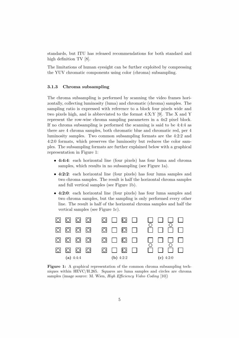
The chroma subsampling is performed by scanning the video frames hori-zontally, collecting luminosity (luma) and chromatic (chroma) samples. Thesampling ratio is expressed with reference to a block four pixels wide andtwo pixels high, and is abbreviated to the format 4:X:Y [9]. The X and Yrepresent the row-wise chroma sampling parameters in a 4x2 pixel block.If no chroma subsampling is performed the scanning is said to be 4:4:4 asthere are 4 chroma samples, both chromatic blue and chromatic red, per 4luminosity samples. Two common subsampling formats are the 4:2:2 and4:2:0 formats, which preserves the luminosity but reduces the color sam-ples. The subsampling formats are further explained below with a graphicalrepresentation in Figure 1:

• 4:4:4: each horizontal line (four pixels) has four luma and chromasamples, which results in no subsampling (see Figure 1a).

• 4:2:2: each horizontal line (four pixels) has four luma samples andtwo chroma samples. The result is half the horizontal chroma samplesand full vertical samples (see Figure 1b).

• 4:2:0: each horizontal line (four pixels) has four luma samples andtwo chroma samples, but the sampling is only performed every otherline. The result is half of the horizontal chroma samples and half thevertical samples (see Figure 1c).

(a) 4:4:4 (b) 4:2:2 (c) 4:2:0

Figure 1: A graphical representation of the common chroma subsampling tech-niques within HEVC/H.265. Squares are luma samples and circles are chromasamples (image source: M. Wien, High Efficiency Video Coding [10])

5

The result of chroma subsampling is a decreased picture color resolution andthe image quality will be affected on a pixel level, but the human eye willbarely be able to notice it from a regular viewing distance due to it beingmore sensitive to light than color [10, p. 35]. The 4:2:0 is commonly used invideo compression and is implemented in both AVC and HEVC [3, 4]. Eachsample is typically repre sented by eight bits (0-255) of precision, but tenbits (0-1024) are also used within HEVC [4].

3.2 Video coding

Video coding is a compression method used to find redundant information ina video sequence and compress it efficiently to achieve smaller video file sizesresulting in less bits in the video bitstream. Video coding include encodingand decoding, where the encoder compresses the video and encodes it intoa bitstream which is received by the decoder to reconstruct the compressedvideo sequence.

3.2.1 Video coding system

The basic video coding system consists of seven component blocks, as seenin Figure 2. The video coding system component blocks are similar formany video coding standards, but each block can have different techniquesand methods implemented, and improvements are made for each new videocoding standard.

• Source: the video sequence to be coded

• Pre-processing: video sequence operations, e.g. trimming or crop-ping, performed on the video to be coded.

• Encoding: encodes the compressed video to a bitstream.

• Transmission: sends the bitstream over a channel, e.g. a network.

• Decoding: transform the encoded bitstream back to a video format.

• Post-processing: operations to enhance the video, e.g. color or con-trast adjustments.

• Display: presents the video in a viewable format, e.g. on a display.

6

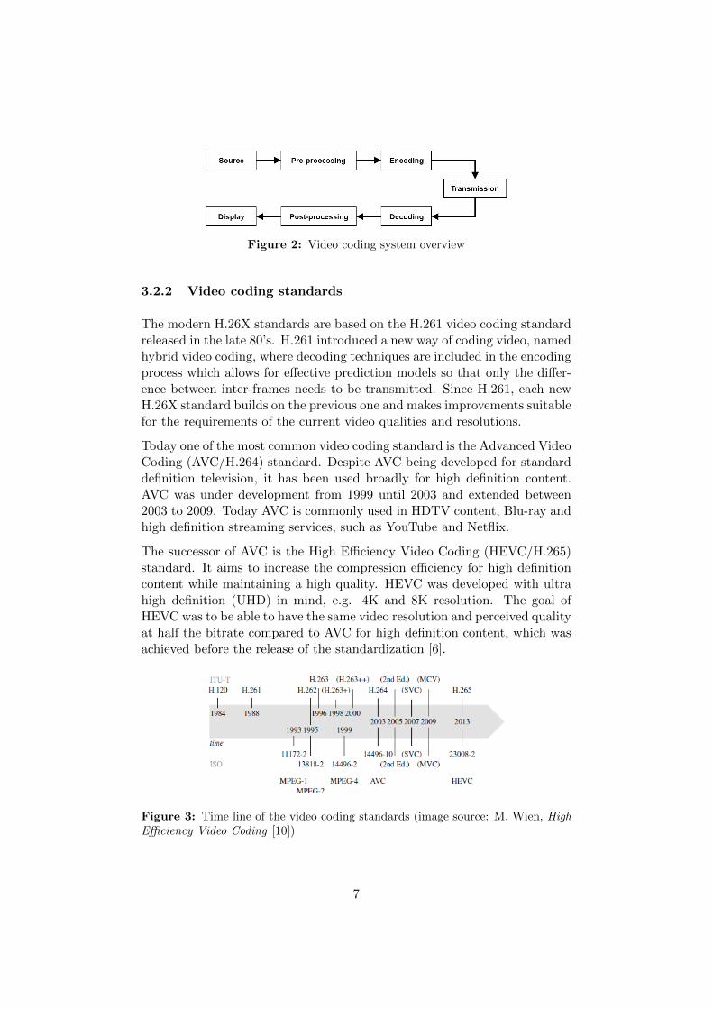
Figure 2: Video coding system overview

3.2.2 Video coding standards

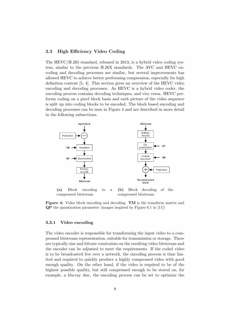
The modern H.26X standards are based on the H.261 video coding standardreleased in the late 80’s. H.261 introduced a new way of coding video, namedhybrid video coding, where decoding techniques are included in the encodingprocess which allows for effective prediction models so that only the differ-ence between inter-frames needs to be transmitted. Since H.261, each newH.26X standard builds on the previous one and makes improvements suitablefor the requirements of the current video qualities and resolutions.

Today one of the most common video coding standard is the Advanced VideoCoding (AVC/H.264) standard. Despite AVC being developed for standarddefinition television, it has been used broadly for high definition content.AVC was under development from 1999 until 2003 and extended between2003 to 2009. Today AVC is commonly used in HDTV content, Blu-ray andhigh definition streaming services, such as YouTube and Netflix.

The successor of AVC is the High Efficiency Video Coding (HEVC/H.265)standard. It aims to increase the compression efficiency for high definitioncontent while maintaining a high quality. HEVC was developed with ultrahigh definition (UHD) in mind, e.g. 4K and 8K resolution. The goal ofHEVC was to be able to have the same video resolution and perceived qualityat half the bitrate compared to AVC for high definition content, which wasachieved before the release of the standardization [6].

Figure 3: Time line of the video coding standards (image source: M. Wien, HighEfficiency Video Coding [10])

7

3.3 High Efficiency Video Coding

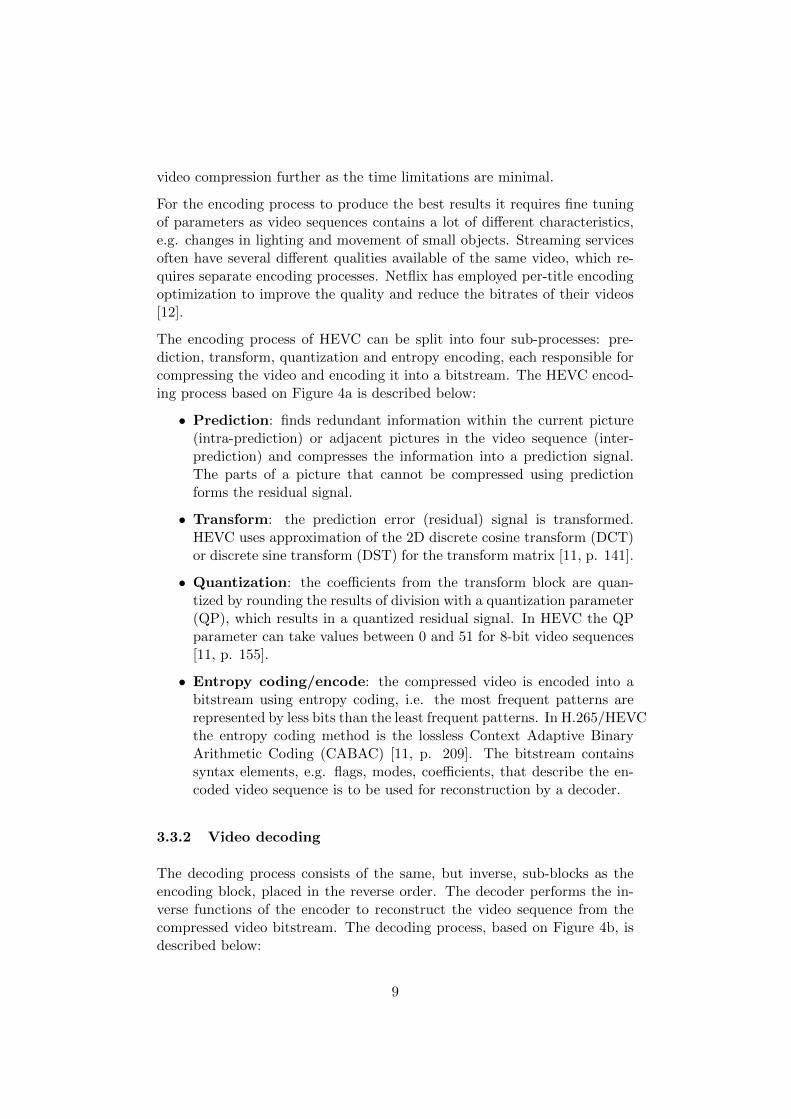
The HEVC/H.265 standard, released in 2013, is a hybrid video coding sys-tem, similar to the previous H.26X standards. The AVC and HEVC en-coding and decoding processes are similar, but several improvements hasallowed HEVC to achieve better performing compression, especially for highdefinition content [5, 4]. This section gives an overview of the HEVC videoencoding and decoding processes. As HEVC is a hybrid video coder, theencoding process contains decoding techniques, and vice versa. HEVC per-forms coding on a pixel block basis and each picture of the video sequenceis split up into coding blocks to be encoded. The block based encoding anddecoding processes can be seen in Figure 4 and are described in more detailin the following subsections.

(a) Block encoding to acompressed bitstream

(b) Block decoding of thecompressed bitstream

Figure 4: Video block encoding and decoding. TM is the transform matrix andQP the quantization parameter (images inspired by Figure 6.1 in [11])

3.3.1 Video encoding

The video encoder is responsible for transforming the input video to a com-pressed bitstream representation, suitable for transmission or storage. Thereare typically size and bitrate constraints on the resulting video bitstream andthe encoder can be adjusted to meet the requirements. If the coded videois to be broadcasted live over a network, the encoding process is time lim-ited and required to quickly produce a highly compressed video with goodenough quality. On the other hand, if the video is required to be of thehighest possible quality, but still compressed enough to be stored on, forexample, a blu-ray disc, the encoding process can be set to optimize the

8

video compression further as the time limitations are minimal.

For the encoding process to produce the best results it requires fine tuningof parameters as video sequences contains a lot of different characteristics,e.g. changes in lighting and movement of small objects. Streaming servicesoften have several different qualities available of the same video, which re-quires separate encoding processes. Netflix has employed per-title encodingoptimization to improve the quality and reduce the bitrates of their videos[12].

The encoding process of HEVC can be split into four sub-processes: pre-diction, transform, quantization and entropy encoding, each responsible forcompressing the video and encoding it into a bitstream. The HEVC encod-ing process based on Figure 4a is described below:

• Prediction: finds redundant information within the current picture(intra-prediction) or adjacent pictures in the video sequence (inter-prediction) and compresses the information into a prediction signal.The parts of a picture that cannot be compressed using predictionforms the residual signal.

• Transform: the prediction error (residual) signal is transformed.HEVC uses approximation of the 2D discrete cosine transform (DCT)or discrete sine transform (DST) for the transform matrix [11, p. 141].

• Quantization: the coefficients from the transform block are quan-tized by rounding the results of division with a quantization parameter(QP), which results in a quantized residual signal. In HEVC the QPparameter can take values between 0 and 51 for 8-bit video sequences[11, p. 155].

• Entropy coding/encode: the compressed video is encoded into abitstream using entropy coding, i.e. the most frequent patterns arerepresented by less bits than the least frequent patterns. In H.265/HEVCthe entropy coding method is the lossless Context Adaptive BinaryArithmetic Coding (CABAC) [11, p. 209]. The bitstream containssyntax elements, e.g. flags, modes, coefficients, that describe the en-coded video sequence is to be used for reconstruction by a decoder.

3.3.2 Video decoding

The decoding process consists of the same, but inverse, sub-blocks as theencoding block, placed in the reverse order. The decoder performs the in-verse functions of the encoder to reconstruct the video sequence from thecompressed video bitstream. The decoding process, based on Figure 4b, isdescribed below:

9

• Entropy decode: the CABAC encoded bitstream is decoded to pro-duce the syntax elements (flags, modes, coefficients) to be used in thevideo sequence reconstruction process.

• De-quantization: the quantized transform coefficients of the residualsignal are scaled up by multiplication with the quantization parameter(QP).

• Inverse transform: the scaled coefficients are inverse transformed.HEVC specifies an approximation of the 2D Inverse Discrete CosineTransform (IDCT) or Inverse Discrete Sine Transform (IDST) for theinverse transform matrix [11, p. 143].

• Prediction: the parts of the video sequence that has been compressedusing either intra- or inter-prediction methods is reconstructed by com-bining the prediction and residual signals.

3.3.3 Video coding units

The individual pictures of a video sequence to be coded are split up intonon-overlapping pixel blocks, and is used by both AVC and HEVC. HEVCimplements a new type of pixel block, the coding tree unit (CTU), to replacethe largest coding unit of AVC, the macroblock (16x16 pixels). The CTUcan vary in size (16x16, 32x32 or 64x64) and is always the same for a fullvideo sequence. The next generation video coding standard is likely tosupport CTU sizes up to 128x128 pixels, as it is supported in JVET JEM4.1 [7].

Each CTU block can be divided into sub-blocks of different types and sizes.The size of each sub-block is determined by the picture information withinthe CTU. Blocks that contain many small details are typically divided intosmaller sub-blocks to retain the fine details, while the sub-blocks can belarger in locations where there are fewer details, e.g. a white wall or a bluesky.

The relation between blocks and sub-blocks is represented by a quadtreedata structure, where the CTU is the root of the coding units (CU). Anexample of how a CTU can be split up into a CU quadtree can be seen inFigure 5. Each CU contains three blocks for each color component, i.e. oneblock for luminosity (Y), chromatic blue (Cb or U) and chromatic red (Cror V). The location of the luminosity blocks are used to derive the locationof the corresponding chroma blocks, with some potential deviation for thechroma components depending on the chroma subsampling setting [10, p.115].

10

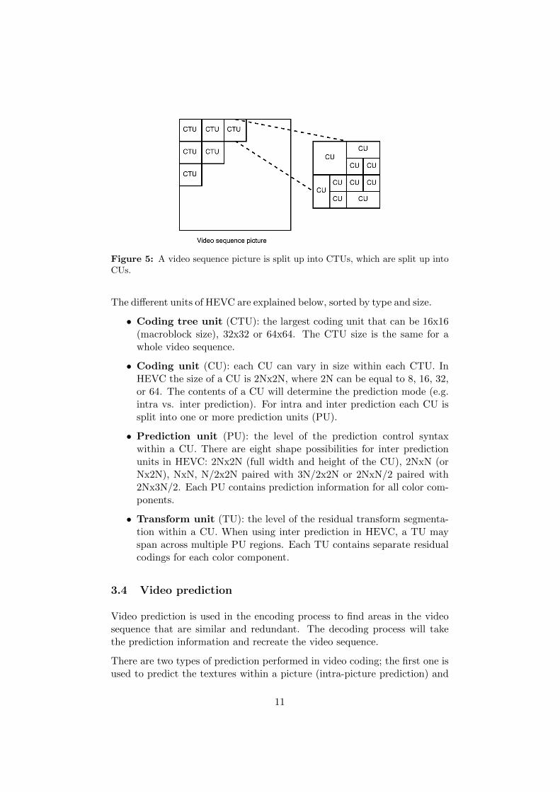
Figure 5: A video sequence picture is split up into CTUs, which are split up intoCUs.

The different units of HEVC are explained below, sorted by type and size.

• Coding tree unit (CTU): the largest coding unit that can be 16x16(macroblock size), 32x32 or 64x64. The CTU size is the same for awhole video sequence.

• Coding unit (CU): each CU can vary in size within each CTU. InHEVC the size of a CU is 2Nx2N, where 2N can be equal to 8, 16, 32,or 64. The contents of a CU will determine the prediction mode (e.g.intra vs. inter prediction). For intra and inter prediction each CU issplit into one or more prediction units (PU).

• Prediction unit (PU): the level of the prediction control syntaxwithin a CU. There are eight shape possibilities for inter predictionunits in HEVC: 2Nx2N (full width and height of the CU), 2NxN (orNx2N), NxN, N/2x2N paired with 3N/2x2N or 2NxN/2 paired with2Nx3N/2. Each PU contains prediction information for all color com-ponents.

• Transform unit (TU): the level of the residual transform segmenta-tion within a CU. When using inter prediction in HEVC, a TU mayspan across multiple PU regions. Each TU contains separate residualcodings for each color component.

3.4 Video prediction

Video prediction is used in the encoding process to find areas in the videosequence that are similar and redundant. The decoding process will takethe prediction information and recreate the video sequence.

There are two types of prediction performed in video coding; the first one isused to predict the textures within a picture (intra-picture prediction) and

11

the other is used to predict textures between adjacent pictures (inter-pictureprediction) in the video sequence.

3.4.1 Intra-picture prediction

The intra-picture prediction is performed to compress the information withina single picture. The texture areas of the picture that have similar structurecan be compressed by having reference areas predict what textures shouldbe between them. The compression efficiency of the intra-picture predictionis therefore dependent on the areas in the picture. A solid colored picturecan be more efficiently compressed by intra prediction than a picture witha lot of small details that differ throughout the picture. The intra-pictureprediction in video compression is similar to how different image processingtools compress images, e.g. JPEG compression.

3.4.2 Inter-picture prediction

Inter-picture prediction (also called motion compensated prediction) is usedto find redundant information between adjacent picture frames in a videosequence and describe movement of textures as motion vectors. The interprediction is typically performed only on the luminance component (Y inYCbCr/YUV) as it contains the grayscale texture details of the video. Interprediction include motion estimation (ME) to find suitable motion vectorsand motion compensation (MC) to apply the estimated motion vectors toreconstruct the video sequence. Video sequences typically have differenttypes of movement involved, for example objects in motion and camerapanning.

Motion estimation and compensation Motion estimation (ME) is per-formed by the encoder to search for matching pixel blocks in previous orfuture pictures of the video sequence. The movement between each pictureframe is typically small, especially for high framerate video sequences, sothe search area to find the same pixel block is often limited (see Figure 6).The best matching pixel block in an adjacent picture will have its movementrepresented by a motion vector that describes the direction and length ofthe movement, and a prediction error signal, often referred to as the resid-ual signal, to describe the parts of the block that could not be correctlypredicted. The decoder receives the motion vectors and residual signal aspart of the video bitstream and reconstructs the video sequence using mo-tion compensation (MC) to apply the motion vectors. The residual signal isexpensive to transmit as it contains information to correct the ME motionvector prediction signal. To reduce the impact of the residual signal it is

12

typically compressed using transform methods, e.g. DCT, and quantizationto reduce the cost of transmission, but it is still expensive in comparison toperfect prediction signals.

Figure 6: Motion estimation search to find the best match for the current blockwithin the search range (image source: M. Wien, High Efficiency Video Coding[10])

Uni- and bi-prediction Motion estimation can be performed from eitherone reference picture, i.e. uni-prediction, or from two reference pictures, i.e.bi-prediction. An example of how picture data is predicted from one orseveral reference pictures can be seen in Figure 7, where the picture poccontains predicted pixel blocks from several reference pictures.

Figure 7: Unidirectional and bidirectional prediction of the picture number poc(picture order count) in the video sequence (image source: M. Wien, High EfficiencyVideo Coding [10])

All the pictures that have the potential to be used as reference pictures forinter prediction are stored in a reference picture set (RPS). For each picturethat is to be inter-predicted, a subset of the RPS is placed in a referencepicture list to hold the reference pictures for the current picture to be coded.For uni-prediction there is only one reference list active (List0 or List1) whiletwo lists (List0 and List1) are active for bi-prediction. The two referencepicture lists contains potential reference pictures for the current frame tobe encoded but the two lists order the reference pictures differently. List0

13

contains: short-term before, short-term after and long-term pictures, whileList1 contains: short-term after, short-term before and long-term pictures.The short term reference pictures are close to the picture to be predictedwhile the long-term reference pictures can be further away. Typically theframes that have not been inter-predicted will serve as long-term referencepictures.

Bi-prediction is effective for video sequences where there is a lot of fastmovement, camera panning, zooming in or out and scene changes. The bi-prediction typically builds on the result of uni-prediction and attempts toimprove it and the resulting bi-prediction is only used if it is an improve-ment. First the best block from the forward prediction candidate list (List0)is selected. Then the weighted summation of the best block and several can-didate backward prediction blocks are calculated. The opposite order offinding blocks, e.g. List1 before List0, has been considered in combinationwith a bi-prediction skip method [13].

The block combinations with the smallest rate-distortion cost (RDC) is thenused for the bi-prediction. The process is called rate-distortion optimization(RDO) and optimizes the quality loss, i.e. distortion, versus the bit rate.The quality is typically measured comparing the sum-of-square error (SSE)or sum-of-absolute difference (SAD), both of which are implemented as partof the RDO in AVC and HEVC encoders [10, p. 66]. There are modelsbetter at representing the human perceived video quality, but they are oftencomputationally complex which makes them unsuitable for the video encod-ing process [14]. There have been suggestions for better RDO based on thestructural similarity (SSIM) which yielded better results than SSE and SAD[15]. The most common video quality measurement methods used in videocoding are presented in section 3.6.

Both the uni- and bi-prediction modes can weigh the reference pictures to becombined using weighted prediction, where a weight and an offset is appliedto the MC blocks to fade or blend the predictions [10, p. 183].

3.4.3 Sub-pixel prediction

Fine movement changes between adjacent video sequence pictures benefitsfrom having the motion vectors to be coded on a subpixel level. The sub-pixel movement offers smoother transitions using fractional pixel sampleinterpolation between the integer pixels displayed on monitors. Both AVCand HEVC support half- and quarter-pixel motion using interpolation fil-tering.

The higher precision motion requires more bits for the motion vectors andmore processing power to encode and decode, but can result in a more accu-

14

rate representation of motion and a reduced residual signal as the predictionsignal quality is increased [3].

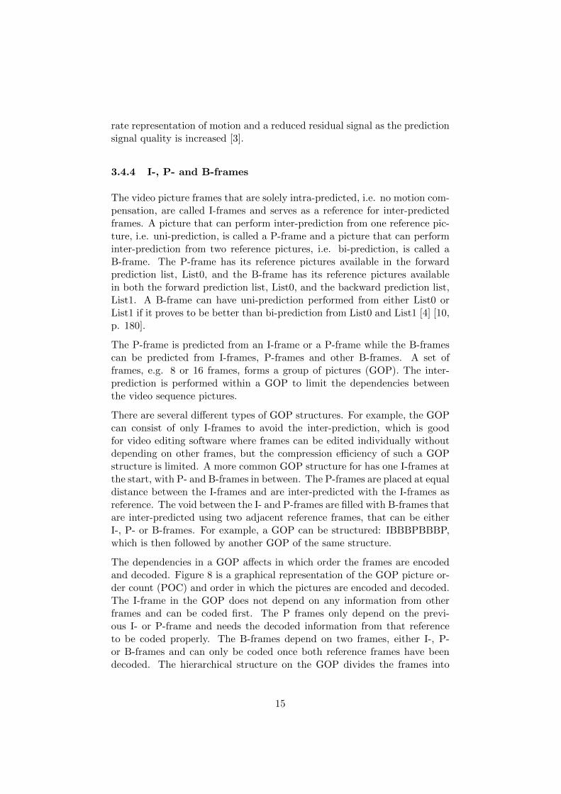
3.4.4 I-, P- and B-frames

The video picture frames that are solely intra-predicted, i.e. no motion com-pensation, are called I-frames and serves as a reference for inter-predictedframes. A picture that can perform inter-prediction from one reference pic-ture, i.e. uni-prediction, is called a P-frame and a picture that can performinter-prediction from two reference pictures, i.e. bi-prediction, is called aB-frame. The P-frame has its reference pictures available in the forwardprediction list, List0, and the B-frame has its reference pictures availablein both the forward prediction list, List0, and the backward prediction list,List1. A B-frame can have uni-prediction performed from either List0 orList1 if it proves to be better than bi-prediction from List0 and List1 [4] [10,p. 180].

The P-frame is predicted from an I-frame or a P-frame while the B-framescan be predicted from I-frames, P-frames and other B-frames. A set offrames, e.g. 8 or 16 frames, forms a group of pictures (GOP). The inter-prediction is performed within a GOP to limit the dependencies betweenthe video sequence pictures.

There are several different types of GOP structures. For example, the GOPcan consist of only I-frames to avoid the inter-prediction, which is goodfor video editing software where frames can be edited individually withoutdepending on other frames, but the compression efficiency of such a GOPstructure is limited. A more common GOP structure for has one I-frames atthe start, with P- and B-frames in between. The P-frames are placed at equaldistance between the I-frames and are inter-predicted with the I-frames asreference. The void between the I- and P-frames are filled with B-frames thatare inter-predicted using two adjacent reference frames, that can be eitherI-, P- or B-frames. For example, a GOP can be structured: IBBBPBBBP,which is then followed by another GOP of the same structure.

The dependencies in a GOP affects in which order the frames are encodedand decoded. Figure 8 is a graphical representation of the GOP picture or-der count (POC) and order in which the pictures are encoded and decoded.The I-frame in the GOP does not depend on any information from otherframes and can be coded first. The P frames only depend on the previ-ous I- or P-frame and needs the decoded information from that referenceto be coded properly. The B-frames depend on two frames, either I-, P-or B-frames and can only be coded once both reference frames have beendecoded. The hierarchical structure on the GOP divides the frames into

15

layers, also known as temporal layers. The low temporal layers of a GOPhas little to no dependencies and are typically I- and P-frames, while thehigher layers, often B-frames, depends on reference pictures from the lowertemporal layers.

Figure 8: A typical GOP structure with I-, P- and B-frames included (imagesource: JCTVC-Software Manual, as part of JEM 4.1 [7]). Picture order count(POC) represents the order in which the pictures are displayed.

3.5 Picture and video signal processing

The video coding process performs digital signal processing such as trans-form methods and filtering. The pictures in a video sequence can individu-ally be described by two dimensional sinusoidal signals that represents thepixel intensity variations.

3.5.1 Pictures as two dimensional signals

The pixel rows and columns of a picture can be translated to horizontaland vertical digital signals. Each signal describes the changes in pixel in-tensity, i.e. color and luminosity. The signal amplitude represents the in-tensity and the signal frequency the intensity transition. A blank picturewith no changes in pixel intensity is represented by a constant two dimen-sional signal. A picture with slow or gradient changes in pixel intensityresults in low frequency signals, while a picture with lots of variation andfast intensity transitions results in high frequency signals. There are twotypes of frequencies that can be measured in pictures in a video sequence;spatial and temporal frequency. The spatial frequency represents the pixelintensity transitions within a picture, while the temporal frequency repre-sents the pixel intensity transitions between adjacent pictures in a videosequence.

To get a better understanding of the spatial two dimensional discrete sig-nals they can be transformed and viewed in the frequency domain using thetwo dimensional discrete Fourier transform (DFT), or the more efficient fast

16

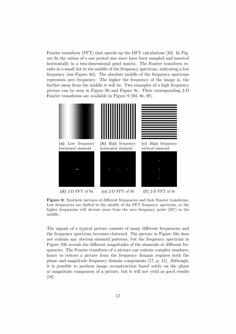
Fourier transform (FFT) that speeds up the DFT calculations [16]. In Fig-ure 9a the values of a one period sine wave have been sampled and insertedhorizontally in a two-dimensional pixel matrix. The Fourier transform re-sults in a small dot in the middle of the frequency spectrum, indicating a lowfrequency (see Figure 9d). The absolute middle of the frequency spectrumrepresents zero frequency. The higher the frequency of the image is, thefurther away from the middle it will be. Two examples of a high frequencypicture can be seen in Figure 9b and Figure 9c. Their corresponding 2-DFourier transforms are available in Figure 9 (9d, 9e, 9f).

(a) Low frequencyhorizontal sinusoid

(b) High frequencyhorizontal sinusoid

(c) High frequencyvertical sinusoid

(d) 2-D FFT of 9a (e) 2-D FFT of 9b (f) 2-D FFT of 9c

Figure 9: Synthetic pictures of different frequencies and their Fourier transforms.Low frequencies are shifted to the middle of the FFT frequency spectrum, so thehigher frequencies will deviate more from the zero frequency point (DC) in themiddle.

The signals of a typical picture consists of many different frequencies andthe frequency spectrum becomes cluttered. The picture in Figure 10a doesnot contain any obvious sinusoid patterns, but the frequency spectrum inFigure 10b reveals the different magnitudes of the sinusoids at different fre-quencies. The Fourier transform of a picture can contain complex numbers,hence to restore a picture from the frequency domain requires both thephase and magnitude frequency domain components [17, p. 11]. Although,it is possible to perform image reconstruction based solely on the phaseor magnitude component of a picture, but it will not yield as good results[18].

17

(a) A typical grayscale pic-ture

(b) 2-D FFT magnitude of10a

Figure 10: An example of how a picture can look in the two-dimensional spatialdomain and frequency domain, using the two dimensional Fourier transform.

3.5.2 Image arithmetic to combine pictures

Image arithmetic can be used for noise reduction by adding video frames to-gether and motion detection by subtracting frames [19, p. 43]. Adding twoimages together is not straightforward when information needs to be pre-served, e.g. in grayscale pictures the white is the absolute highest valueand when adding black and white together only the white will be pre-served, and therefore averaging pictures into a combined picture is com-monly used.

Pixel addition Adding a complete white picture (maximum luminosityintensity) to a complete black image (minimum luminosity intensity) willresult in a white image, as it is basically 1+0=1. MATLAB has a built infunction to add images together, imadd, which performs pixel addition oftwo image matrices:

Pr[x, y] = P1[x, y] + P2[x, y] (1)

Using the imadd on two images (16x16 pixels), Figure 11a and Figure 11b,yields the result visible in Figure 11c. The white areas (max luminosityvalue) of the two added pictures takes over in the resulting picture and thecharacteristics of the first image 11a is only preserved in the black areas ofthe second image 11b.

Addition in the frequency domain It is possible to combine picturecharacteristics by adding the Fourier transforms of two pictures. The result

18

of addition in the frequency domain is the same as addition in the spatialdomain, hence will yield the same result as in Figure 11c.

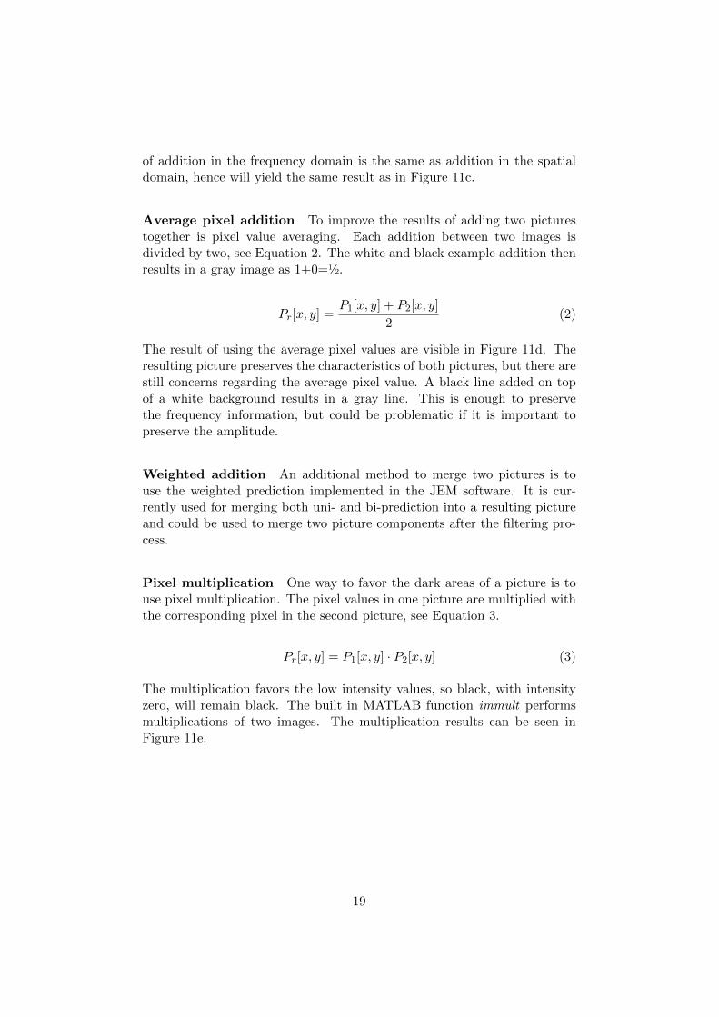
Average pixel addition To improve the results of adding two picturestogether is pixel value averaging. Each addition between two images isdivided by two, see Equation 2. The white and black example addition thenresults in a gray image as 1+0=1⁄2.

Pr[x, y] =P1[x, y] + P2[x, y]

2(2)

The result of using the average pixel values are visible in Figure 11d. Theresulting picture preserves the characteristics of both pictures, but there arestill concerns regarding the average pixel value. A black line added on topof a white background results in a gray line. This is enough to preservethe frequency information, but could be problematic if it is important topreserve the amplitude.

Weighted addition An additional method to merge two pictures is touse the weighted prediction implemented in the JEM software. It is cur-rently used for merging both uni- and bi-prediction into a resulting pictureand could be used to merge two picture components after the filtering pro-cess.

Pixel multiplication One way to favor the dark areas of a picture is touse pixel multiplication. The pixel values in one picture are multiplied withthe corresponding pixel in the second picture, see Equation 3.

Pr[x, y] = P1[x, y] · P2[x, y] (3)

The multiplication favors the low intensity values, so black, with intensityzero, will remain black. The built in MATLAB function immult performsmultiplications of two images. The multiplication results can be seen inFigure 11e.

19

(a) Picture A (b) Picture B

(c) A + B (d) (A + B) / 2 (e) A .* B

Figure 11: Merging of two synthetic pictures (11a and 11b)

3.5.3 Two dimensional filtering of pictures

The digital signals of a picture can be filtered using digital filters, e.g. finiteimpulse response (FIR) or infinite impulse response (IIR) filters. Both FIRand IIR filters can be used for two dimensional filtering, but the FIR filteris preferable as it is guaranteed to be stable and can be designed to havea linear phase, which is a property useful in image processing as all signalswill be equally phase shifted [20]. The basic use of two dimensional filtersfor image processing are blurring or sharpening of images. More advancedfiltering techniques can be used to extract image information, e.g. edgedetection or texture classification [21, 22].

To filter a two dimensional signal the filter implementation needs to operateon both vertical and horizontal signals. A one dimensional filter can beconverted to a two dimensional filter by multiplying the filter coefficientsvector with the transpose vector of the same coefficients. The resulting twodimensional filter has the same filtering behavior as the one dimensionalfilter used to filter the horizontal and the vertical signals sequentially, whichis how the interpolation filtering within JEM is performed.

There are other ways of converting a one dimensional filter to two dimen-sions, for example by frequency transformation. The frequency transforma-tion is able to capture the one dimensional characteristics and convertingthem to a circularly symmetric two dimensional filter. The McClellan fre-quency transformation has been proven to be a viable option to transform

20

1-D FIR filters to 2-D FIR filters [23].

The two dimensional filtering of a picture can be performed in the spatialdomain or the frequency domain. Filtering in the spatial domain is per-formed by convolution between the signal and the filter impulse response,see Equation 4 where the picture pixel array, a, is convolved with the 2-Dfilter impulse response, h.

c[m,n] = a[m,n]⊗ h[m,n] =J0∑

i=−J0

J0∑j=−J0

a[m− i, n− j] · h[i, j] (4)

Filtering in the frequency domain is performed by Fourier transforming thepicture to the frequency domain and multiplying it with the filter transferfunction, i.e. the Fourier transformed impulse response, as displayed inEquation 5 where the Fourier transform of the picture pixel array, A, ismultiplied with the filter transfer function, H. It is possible to design idealfilters in the frequency domain that filters out desired frequency rangesperfectly. The problem with ideal filters is that when the filtered pictureis transformed back to the spatial domain it will contain ringing artifacts.An ideal filter transfer function, e.g. a box, transformed back to the spatialdomain results in a cardinale sine function, sinc, impulse response whichintroduces a ringing effect in the spatial domain [19, p. 167].

c[m,n] = F−1(F(a[m,n]) · F(h[m,n])) = F−1(A[m,n] ·H[m,n]) (5)

Low pass and high pass filters The typical filters used for picture filtersare low pass and high pass filters. A low pass filter applied on a picture willfilter out the high frequencies, e.g. small details, and typically results in ablurry version of the original picture. One example of low pass filter usedfor image processing is the Gaussian blur filter. In opposite, a high passfilter will filter out the low frequencies and only preserve the small details,such as edges which can be used for sharpening the original picture.

The low pass and high pass filter characteristics are the opposites of eachother, both in one and two dimensions. If a picture has been low pass filteredit is possible to extract the remaining high frequencies by subtracting theoriginal picture with the low pass filtered picture, or in other words, subtractthe low pass filter from an all pass filter to achieve a high pass filter [24, p.272].

Some common filter design methods used in digital signal processing in-clude the Gaussian, Butterworth, Chebyshev, elliptic, bilateral and notchfilters.

21

Separable filters Two-dimensional filters that can be separated into 1-Dfilters that preserves the horizontal and vertical signal filtering behavior arecalled separable filters [24, p. 404]. A common separable filter is the 2-DGaussian filter that can be separated into a 1-D Gaussian filter, which is oneof the reasons for being a common image processing filter [24, p. 406].

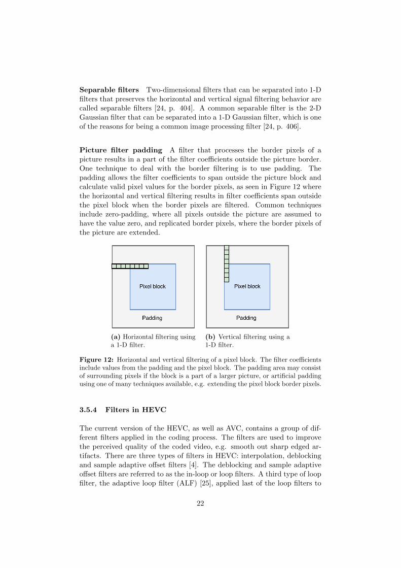
Picture filter padding A filter that processes the border pixels of apicture results in a part of the filter coefficients outside the picture border.One technique to deal with the border filtering is to use padding. Thepadding allows the filter coefficients to span outside the picture block andcalculate valid pixel values for the border pixels, as seen in Figure 12 wherethe horizontal and vertical filtering results in filter coefficients span outsidethe pixel block when the border pixels are filtered. Common techniquesinclude zero-padding, where all pixels outside the picture are assumed tohave the value zero, and replicated border pixels, where the border pixels ofthe picture are extended.

(a) Horizontal filtering usinga 1-D filter.

(b) Vertical filtering using a1-D filter.

Figure 12: Horizontal and vertical filtering of a pixel block. The filter coefficientsinclude values from the padding and the pixel block. The padding area may consistof surrounding pixels if the block is a part of a larger picture, or artificial paddingusing one of many techniques available, e.g. extending the pixel block border pixels.

3.5.4 Filters in HEVC

The current version of the HEVC, as well as AVC, contains a group of dif-ferent filters applied in the coding process. The filters are used to improvethe perceived quality of the coded video, e.g. smooth out sharp edged ar-tifacts. There are three types of filters in HEVC: interpolation, deblockingand sample adaptive offset filters [4]. The deblocking and sample adaptiveoffset filters are referred to as the in-loop or loop filters. A third type of loopfilter, the adaptive loop filter (ALF) [25], applied last of the loop filters to

22

improve the filtering results was evaluated during the development of HEVCbut never implemented in the HEVC release.

• Interpolation filters are used within the inter prediction process tosmooth out the sub-pixel motion vectors to an integer pixel repre-sentation. HEVC increased the number of filter coefficients for theinterpolation filters from 6 to 8 for luma and 2 to 4 for chroma.

• Deblocking filters are used for smoothing blocking artifacts in thecoded video to improve the perceived quality. The blocking artifactsare results of the block-wise video coding, e.g. prediction blocks. Thefilter is applied on the edges between the block coding units.

• Sample adaptive offset (SAO) filters are applied after the deblock-ing filter and is used to improve the picture restoration. The filteringis performed on a CTU basis. The SAO filter was first introducedin the HEVC standard and can be applied on top of previous codingstandards.

The interpolation filter coefficients, i.e. filter taps, in HEVC are separableand scaled up by a factor of 64 and rounded to the nearest integer, hence theresults of the filtering process are scaled by 64 and requires normalization.The scaled up results are normalized by right-shifting by the input video bitdepth minus two [26]. For example, a video sequence of bit depth 8-bit willhave its filter results shifted to the right by 6, while a 10-bit video sequencewill have its filter results shifted to the right by 8.

Sub-pixel interpolation The prediction of fractional pixel motion vec-tors is achieved by interpolation filtering. The H.264/AVC standard uses a6-tap FIR interpolation filter for the half-pixels and a linear interpolationfor the quarter-pixels. The H.265/HEVC standard uses 7-tap or 8-tap FIRinterpolation filtering which improves the filter response and reproduction ofhigh frequency content, i.e. fine details [26]. The interpolation filter is a FIRfilter with coefficients based on the discrete cosine transform (DCT) and iscalled a DCT-based interpolation filter (DCT-IF). The 1-D filter responsesof both AVC and HEVC can be seen in Figure 13.

23

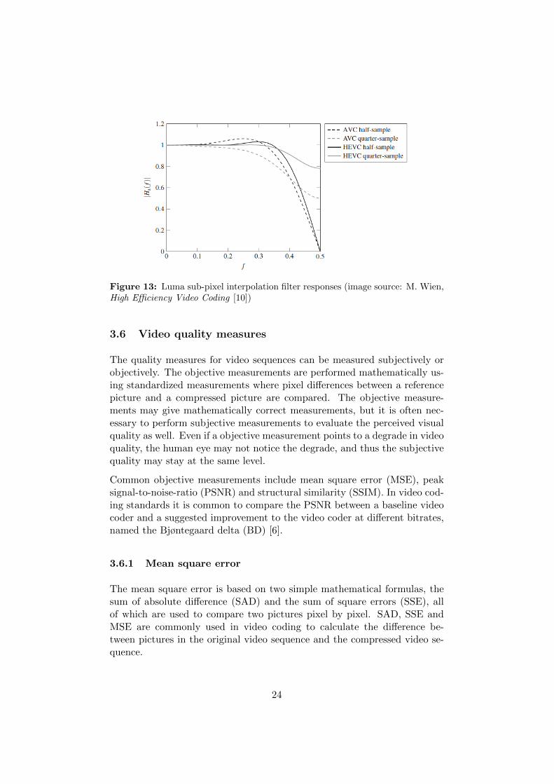
Figure 13: Luma sub-pixel interpolation filter responses (image source: M. Wien,High Efficiency Video Coding [10])

3.6 Video quality measures

The quality measures for video sequences can be measured subjectively orobjectively. The objective measurements are performed mathematically us-ing standardized measurements where pixel differences between a referencepicture and a compressed picture are compared. The objective measure-ments may give mathematically correct measurements, but it is often nec-essary to perform subjective measurements to evaluate the perceived visualquality as well. Even if a objective measurement points to a degrade in videoquality, the human eye may not notice the degrade, and thus the subjectivequality may stay at the same level.

Common objective measurements include mean square error (MSE), peaksignal-to-noise-ratio (PSNR) and structural similarity (SSIM). In video cod-ing standards it is common to compare the PSNR between a baseline videocoder and a suggested improvement to the video coder at different bitrates,named the Bjøntegaard delta (BD) [6].

3.6.1 Mean square error

The mean square error is based on two simple mathematical formulas, thesum of absolute difference (SAD) and the sum of square errors (SSE), allof which are used to compare two pictures pixel by pixel. SAD, SSE andMSE are commonly used in video coding to calculate the difference be-tween pictures in the original video sequence and the compressed video se-quence.

24

The SAD formula sums the absolute pixel value differences, as seen in Equa-tion 6. SSE takes the formula one step further by squaring the pixel valuedifference, as seen in Equation 7. MSE takes the SSE result and calculatesthe mean pixel difference by dividing with the total number of pixels of thepictures that were compared, as seen in Equation 8. The higher the SAD,SSE, and MSE are, the more errors are in the compressed picture. TheMSE measurement can be directly converted to a PSNR ratio presented insection 3.6.2.

The variable A is the decoded compressed picture array and B is the originalpicture array. M and N are the height and width of the pictures.

SAD(A,B) =M−1∑x=0

N−1∑y=0

|B[i, j]−A[i, j]| (6)

SSE(A,B) =M−1∑i=0

N−1∑j=0

(B[i, j]−A([i, j])2 (7)

MSE(A,B) =

∑M−1i=0

∑N−1j=0 (B[i, j]−A[i, j])2

M ·N(8)

3.6.2 Peak signal-to-noise ratio

Peak signal-to-noise ratio (PSNR) is used to compare the quality of a refer-ence picture or sequence of pictures to the compressed version of the samepicture or sequence of pictures. PSNR is commonly used to measure theeffects of video compression and is defined as the ratio between the originalpicture signal and the noise signal introduced using lossy compression [6].The maximum number of pixel values based on the number of bits, B, aresquared and divided by the MSE (see section 3.6.1) of the picture. ThePSNR formula can be seen in Equation 9.

PSNR = 10 · log10(2B − 1)2

MSE(9)

PSNR is measured in the logarithmic unit decibel (dB), and the higher thePSNR, the better quality in comparison to the original picture. For lossycompression at a bit depth of 8 bits the PSNR are typically between 30 dBand 50 dB. PSNR is often used to compare video codecs, but it should notbe seen as a representation of the perceived video quality as the PSNR valuecan vary depending on the image or video content [27].

25

The PSNR can be applied to the separate Y, Cb and Cr components. Atotal PSNR is typically weighed depending on the chroma subsampling. Forexample, the chroma subsampling mode 4:2:0 can have a PSNR formula thatis weighed more heavily on the luma component. An example on how thePSNR calculations can be weighed over the luminosity (Y) and chromaticchannels (Cb and Cr), is available in Equation 10 [6].

PSNRW =6 · PSNRY + PSNRCB

+ PSNRCR

8(10)

3.6.3 Structural similarity

Structural similarity (SSIM) is used to measure the structural similaritiesbetween pictures and predict the perceived quality. SSIM weighs in thestructural distortions such as noise, blocking artifacts, blurring and ring-ing which are easily noticed by the human eye [14]. Although results maydiffer between SSIM and PSNR, they often correlate in image compressionsituations [28]. Changes in luminance, contrast, gamma and spatial shiftsare nonstructural distortions and does not change the structure of the pic-ture.

The mathematical formula of SSIM, in Equation 11, is constructed by threecomponents that measures the difference in luminosity, contrast and struc-ture. If A and B are pictures to be compared using SSIM, l(A,B) com-pares the luminosity, c(A,B) compares the contrast and s(A,B) comparesthe structure. The math behind the formula will not be presented in thisreport as it has been thoroughly explained in other papers [14, 28]. Thethree components can be weighted differently depending on the application,but are usually weighed equally as wl=wc=ws=1.

SSIM(A,B) = [l(A,B)]wl · [c(A,B)]wc · [s(A,B)]ws (11)

3.6.4 Bjøntegaard delta

Bjøntegaard delta (BD) metrics is a standardized measurement used to com-pare the coding efficiencies between video coders over a range of qualitypoints, usually PSNR and bit rates or SSIM and bit rates [10]. The mathe-matical formula for BD-rate (see Equation 12) calculates the area betweentwo plotted lines of quality measurements at different bitrates, as seen inFigure 14, where the quality measurement used is PSNR.

26

∆R(D) =RB(D)−RA(D)

RA(D)(12)

A negative result from the BD calculation means that the tested coder man-aged to produce better results in comparison to the reference coder. Betterresults either means that the same number of bits were used to producehigher quality results or less bits were used to produce similar quality re-sults. In Figure 14 the blue dotted curve produces better results (higherPSNR) with a lower bitrate (fewer bits) and would result in a negativeBD-rate in comparison to the red crossed curve.

Figure 14: Bjøntegaard delta illustration. The area between the curves is calcu-lated to compare the coding efficiencies. (a) BD-PSNR (b) BD-rate (image source:M. Wien, High Efficiency Video Coding [10])

27

4 Method

This section describes the methods used in this project. Pictures are digitalsignals and can be filtered with digital filters. This project aims to makeuse of the different frequency components of the pictures in a video sequenceto improve the inter prediction methods of the video coding system. Thefiltering will be performed on a video picture block level, e.g. CU blocksand sub-blocks.

Prototype filters are implemented in MATLAB while the evaluation is per-formed using the Joint Exploration Model (JEM) [7] that is based on theHEVC reference software model, HM. The final implementation will be lim-ited to fit within the JEM framework and the work will be adjusted to whatis possible within that framework.

4.1 Picture filtering and prediction

The different characteristics of a picture can be separated using digital filters.Low pass filters can be used to extract the low frequency characteristics andhigh pass filters to extract the high frequency characteristics. The frequencyfeatures of pictures depends on their content. Pictures that appear differentmay share certain frequency features.

4.1.1 Improved picture prediction

The separated picture characteristics has potential to be used for betterinter prediction of a video sequence within the video coding process. If theinter prediction, i.e. motion estimation, does not necessarily need to finda perfect match, but a matching low or high frequency characteristic, theresidual signal of the coded video can potentially be reduced.

For example, if there are parts of a video sequence that have low frequencyshadows moving over a high frequency texture the motion estimation mayhave trouble matching the block that is not shadowed with the same blockthat is shadowed in the following frame(s), even though the texture is thesame. By splitting up the block into separate low and high frequency com-ponents it offers the motion estimation to find the matching high frequencyblock texture even if it is shadowed.

28

4.2 Prototype in MATLAB

During the first phase of the project the filtering methods have been testedusing MATLAB and the built in functionality in the image and signal pro-cessing toolbox. The version of MATLAB used for this project is R2016b.

The MATLAB image processing toolbox [29] comes with predefined func-tionality for processing and analyzing pictures including some commonlyused image filtering techniques for image editing, e.g. noise removal, blur-ring and sharpening. Based on that images are two dimensional signals, itis possible to define customized filters using MATLAB’s signal processingtoolbox [30] to filter the pictures.

The prototype includes using 1-D low pass and high pass filters to perform 2-D filtering of pictures. Suitable filters for picture filtering will be prototypedand then implemented as part of the JEM framework.

4.3 Proof of concept in JEM

The prototype low pass and high pass filters from MATLAB have beenimplemented within the JEM framework to be used by the inter pictureprediction. The filtering is performed within motion estimation to find thebest matching filtered blocks and within motion compensation to apply thebest filters.

JEM already has functionality implemented for filtering, i.e. horizontal andvertical interpolation filtering, using 1-D filter coefficients which has beenof benefit for the proof of concept implementation. The version of JEMused in this project is JEM 4.1, based on HM 16.6. JEM is written in C++and released with several Visual Studio version project files. The IDE usedfor implementing the proof of concept within JEM is Visual Studio 2013Professional.

29

5 Related work

The field of video compression is under constant research and improvement.The joint collaborative team on video coding (JCT-VC) group has regularmeetings where researchers from companies from all around the world meetsto discuss video compression research, improvement suggestions and theirresults. If the results are interesting and considered feasible it might be-come a part of the next update of the current, or upcoming, video codingstandard.

The Joint Video Exploration Team (on Future Video coding) (JVET) re-searches the next video coding standard and has overlapping meetings withthe JCT-VC group. JVET develops the next video coding standard refer-ence software Joint Exploration Model (JEM). Their meetings are focusedon extending the HEVC standard to the next generation video coder andimproving the jointly developed JEM software framework.

The method described in this thesis project has not been up for sugges-tion in the standardization meetings or in related academic research papers,making it one of the first in its form. The HEVC standardization have hadseveral filtering techniques suggested and improved, e.g. interpolation, de-blocking and SAO, so there are several filters implemented within the JEMframework, which have inspired the filter implementation.

This thesis focuses on inter prediction and filtering, so the related workresearch has been limited to those specific areas.

5.1 Related JCT-VC research

The JCT-VC meeting documents [31] are publicly available and containsrelated research and improvement proposals for the HEVC standard. Thecollaborators send in technical improvement suggestions and have them eval-uated by the JCT-VC group. In parallel, the JVET group researches im-provements for the next video coding standard, and their meeting documents[32] are publicly available as well.

5.1.1 Filters in video coding

The video coding system contains several filters, e.g. in-loop filters, to im-prove the quality of the coded video. Some of the filters researched arelisted below. Additionally, adaptive loop filters were evaluated during thedevelopment of the HEVC standard, but the added complexity to the cod-ing system was not worth the compression improvements [33]. However,

30

there are adaptive loop filters implemented within the JEM software frame-work.

• High accuracy interpolation filter (HAIF) (A117 [34] / C078) – TOSHIBAThe HAIF is a motion compensation filter, defined as a one dimen-sional FIR filter, to interpolate on a half- and quarter pixel resolutionaccording to fractional pixel motion vector(s). The tool experimentresults points to that the HAIF can achieve good performance withits steep frequency characteristics and long tap length (8-tap and 8/6-tap).

• Non-uniform tap length filtering (NTLF) for bidirectional prediction(D154 [35] / E134 / F315) – TOSHIBAThe worst case of complexity of the interpolation process are twodimensional quarter pixel positions of bidirectional prediction. TheNTLF filter uses both asymmetrical and symmetrical filters and aimsto improve the bidirectional prediction and reduce the computationalcomplexity of the motion compensation interpolation. Original sug-gestion (D154): 12/8 tap DCT-IF and 8/4-tap DCT-IF, this changedin E134 to a 8/6-tap DCT-IF where 8 is the symmetrical filter and6 is the asymmetrical filter. The results show coding losses for theanchor at less than 0.20% and a reduction of the total computationalcomplexities.

• Joint Sub-pixel Interpolation for bi-predicted Motion Compensation(F601 [36]) – MotorolaProposes an interpolation scheme for temporal prediction of predictionunits (PUs) when bi-prediction (B-frame) is used. The optimal filterper reference list (L0 and L1) would depend on the joint sub-pixeloffsets. Some concern was expressed due to the additional complexityand no support was expressed.

5.2 Related scientific papers

5.2.1 Image processing and filters

There has been extensive research within the field of filters in image pro-cessing, e.g. information extraction and enhancements, but nothing thatdirectly relates to the proposed inter prediction method of filtering pictureswithin video sequences.

• Image Features From Phase Congruency [37]The distinct features of an image, such as edges and lines, results inphase changes of the Fourier components. The paper presents a way ofcalculating phase congruency using wavelets and extending it from 1D

31

to 2D signals. The paper discusses the use of low pass, band pass andhigh pass filters for image analysis and argues that high pass filtersshould be used to extract information from images.

• Image Enhancement Techniques using Highpass and Lowpass Filters[38]Both low pass and high pass filters can be used to enhance images.This paper demonstrates the techniques behind image filters such asthe Gaussian and Butterworth filters and compares them to ideal fil-ters. The low pass filter can be used to denoise images, while the highpass filter can be used to preserve edge details.

• Image Analysis by Bidimensional Empirical Mode Decomposition (BEMD)[39]The paper proposes an analysis method for image textures by featureextraction, based on a method called Empirical Mode Decomposition(EMD) [40]. The results of the proposed BEMD method was able toextract different high, mid and low spatial frequency components fromimages. Further analysis of BEMD results was performed in a separatepaper [41].

32

6 Implementation

Two separate implementations, one prototype and one proof-of-concept,have been performed to test the concept of filtering video sequence picturesfor better prediction and video compression. The prototype filter imple-mentation was developed using MATLAB and used for experimentations ofthe low pass and high pass filtering concept. The final implementation ofthe project was implemented within the JEM framework to act as a proof-of-concept to be evaluated in comparison to the original JEM implementa-tion.

6.1 Prototype in MATLAB

The experimental prototype implementation in MATLAB was used to an-alyze pictures and the effects of filtering in both the spatial (pixel) domainand the frequency domain. The prototype implementation made use of boththe signal processing toolbox and the image processing toolbox to analyzeand filter the pictures. The goal of the prototype was to separate the lowand high frequency components of pictures and combine the results to createnew pictures.

6.1.1 Synthetic picture generator

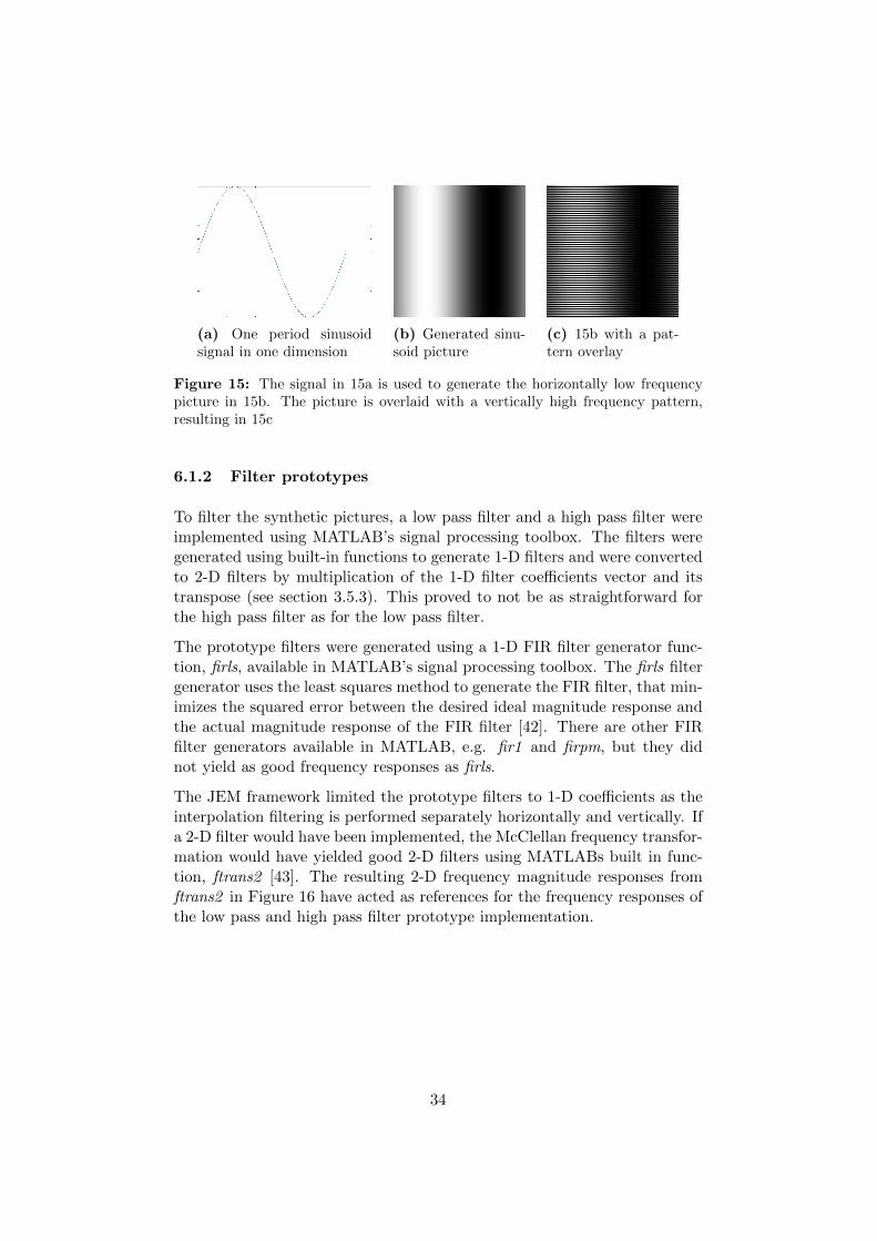
A synthetic picture generator was developed early in the project to be ableto generate picture components of different frequencies. The generator sam-ples one dimensional sinusoidal signals and replicates the data in a NxNpixel matrix, either horizontally or vertically. As an example, a one periodsinusoid (see Figure 15a) was sampled to produce the picture in Figure 15bby extending the one dimensional signal vertically to two dimensions.

In addition a pattern image generator that overlays pictures with a horizon-tal, vertical, diagonal or grid pattern. The patterns are not generated fromsignals, but can be represented by square wave signals as the patterns havesharp edges. By combining the two generators it was possible to create thepicture in Figure 15c. The generated picture consists of a horizontal low fre-quency sinusoid and a vertical high frequency square wave. The generatedsynthetic pictures was used to test the performance of the two dimensionallow pass and high pass filtering prototypes.

33

(a) One period sinusoidsignal in one dimension

(b) Generated sinu-soid picture

(c) 15b with a pat-tern overlay

Figure 15: The signal in 15a is used to generate the horizontally low frequencypicture in 15b. The picture is overlaid with a vertically high frequency pattern,resulting in 15c

6.1.2 Filter prototypes

To filter the synthetic pictures, a low pass filter and a high pass filter wereimplemented using MATLAB’s signal processing toolbox. The filters weregenerated using built-in functions to generate 1-D filters and were convertedto 2-D filters by multiplication of the 1-D filter coefficients vector and itstranspose (see section 3.5.3). This proved to not be as straightforward forthe high pass filter as for the low pass filter.

The prototype filters were generated using a 1-D FIR filter generator func-tion, firls, available in MATLAB’s signal processing toolbox. The firls filtergenerator uses the least squares method to generate the FIR filter, that min-imizes the squared error between the desired ideal magnitude response andthe actual magnitude response of the FIR filter [42]. There are other FIRfilter generators available in MATLAB, e.g. fir1 and firpm, but they didnot yield as good frequency responses as firls.

The JEM framework limited the prototype filters to 1-D coefficients as theinterpolation filtering is performed separately horizontally and vertically. Ifa 2-D filter would have been implemented, the McClellan frequency transfor-mation would have yielded good 2-D filters using MATLABs built in func-tion, ftrans2 [43]. The resulting 2-D frequency magnitude responses fromftrans2 in Figure 16 have acted as references for the frequency responses ofthe low pass and high pass filter prototype implementation.

34

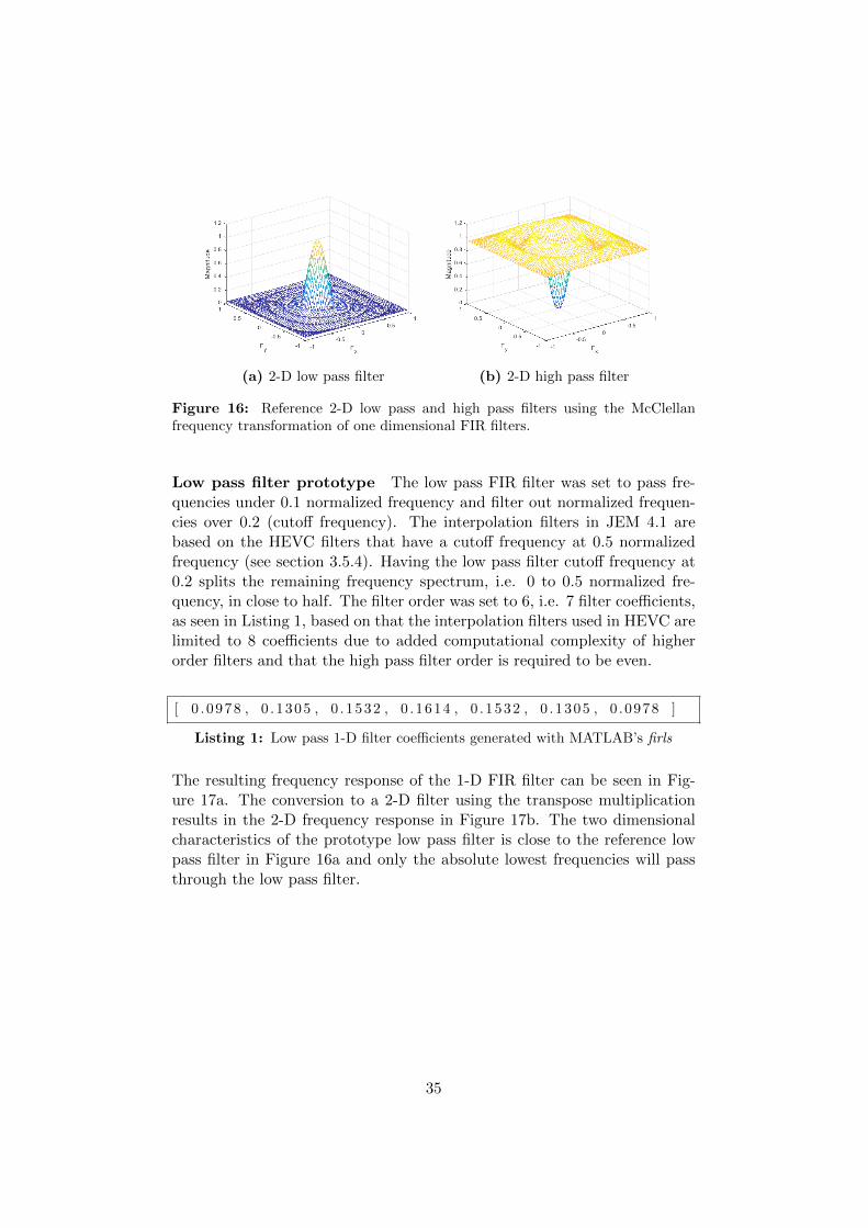
(a) 2-D low pass filter (b) 2-D high pass filter

Figure 16: Reference 2-D low pass and high pass filters using the McClellanfrequency transformation of one dimensional FIR filters.

Low pass filter prototype The low pass FIR filter was set to pass fre-quencies under 0.1 normalized frequency and filter out normalized frequen-cies over 0.2 (cutoff frequency). The interpolation filters in JEM 4.1 arebased on the HEVC filters that have a cutoff frequency at 0.5 normalizedfrequency (see section 3.5.4). Having the low pass filter cutoff frequency at0.2 splits the remaining frequency spectrum, i.e. 0 to 0.5 normalized fre-quency, in close to half. The filter order was set to 6, i.e. 7 filter coefficients,as seen in Listing 1, based on that the interpolation filters used in HEVC arelimited to 8 coefficients due to added computational complexity of higherorder filters and that the high pass filter order is required to be even.

[ 0 . 0978 , 0 .1305 , 0 .1532 , 0 .1614 , 0 .1532 , 0 .1305 , 0 .0978 ]

Listing 1: Low pass 1-D filter coefficients generated with MATLAB’s firls

The resulting frequency response of the 1-D FIR filter can be seen in Fig-ure 17a. The conversion to a 2-D filter using the transpose multiplicationresults in the 2-D frequency response in Figure 17b. The two dimensionalcharacteristics of the prototype low pass filter is close to the reference lowpass filter in Figure 16a and only the absolute lowest frequencies will passthrough the low pass filter.

35

(a) 1-D frequency response of the lowpass filter

(b) 2-D frequency response of thelow pass filter

Figure 17: Frequency responses of a 1-D FIR filter 17a generated using MATLAB’sfirls function converted to a 2-D filter 17b using transpose multiplication of the 1-DFIR filter coefficients.

High pass filter prototype The prototype high pass FIR filter is definedas the opposite of the low pass filter, i.e. to pass frequencies over 0.2 normal-ized frequency and filter out frequencies under 0.1 (cutoff frequency). Thehigh pass filter order was required to be even when generated using the firlsand was set to filter order 6, i.e. 7 filter coefficients Listing 2 to fit withinthe limit of 8 coefficients in JEM 4.1. The resulting frequency response ofthe 1-D FIR filter can be seen in Figure 18a. The conversion to a 2-D filterusing the transpose multiplication results in the 2-D frequency response inFigure 18b.

[−0.0978 ,−0.1305 ,−0.1532 , 0.8386 ,−0.1532 ,−0.1305 ,−0.0978]

Listing 2: High pass 1-D filter coefficients generated with firls

(a) Frequency response of the prototype1-D high pass filter

(b) Frequency response of thetranspose 2-D high pass filter

Figure 18: Frequency responses of a 1-D FIR filter 18a generated using MATLAB’sfirls function, converted to a 2-D filter 18b by transpose multiplication.

36

By analyzing the frequency response of the generated 2-D filter in Figure 18bit became clear that it will filter out several high frequencies, where either thehorizontal or vertical frequency (Fy or Fx) are at zero. A correct high passfilter would be an inverse of a low pass filter where all the high frequenciesare captured, similar to the reference filter in Figure 16b. The followingsection (section 6.1.3) explains how the prototype frequency response wasimproved using the characteristics of the high pass filter.

6.1.3 Improved high pass filtering

To improve the filtering results of the high pass filter it is possible to performseparate vertical and horizontal filtering of the original picture and thenadd the results together. This does not equal to the transpose techniqueused for the first high pass filter prototype, as high pass filters are notseparable.

The frequency response of a 1-D filter in two dimensions is an extension ofthe 1-D frequency response along either the horizontal or vertical axis of thetwo dimensional space. The 1-D frequency response of the high pass filterFigure 18 can be horizontally and vertically extended to two dimensions, asseen in Figure 19a and Figure 19b. To combine the horizontal and verticalfilters, their results can be added together to form a picture that has beenfiltered in two dimensions. The combined frequency response of the verticaland horizontal high pass filters can be seen in Figure 19c.

(a) Horizontal frequencyresponse in 2-D

(b) Vertical frequencyresponse in 2-D

(c) Combination of 19aand 19b (addition)

Figure 19: Frequency responses of a 1-D FIR filter in Figure 18 extended, horizon-tally and vertically, to two dimensions. The addition of the horizontal and verticalfilters creates the frequency response in 19c.

The lowest frequencies are filtered out (blue area), but there are still issueswith the high frequency signals. Purely vertical and horizontal high frequen-cies will be dampened (green areas) in comparison to the frequencies thatare high both vertically and horizontally (yellow areas). The magnitude re-sponse for the diagonally high frequencies are doubled after the addition of

37

the high pass filters, i.e. the maximum magnitude has increased from 1 to2 in Figure 19c.

It is possible to use the two high pass filter prototypes to construct a betterhigh pass filter. The improved high pass filter frequency response in Fig-ure 20b can be subtracted with the frequency response of the first prototypein Figure 20a to create a better high pass filter. The subtraction results ina two dimensional frequency response of a high pass filter, see Figure 20c,which is the opposite of the prototype low pass filter in Figure 21a. Thedifferent high pass filter prototypes are compared and evaluated in section6.1.4.

(a) The frequency re-sponse from Figure 18b

(b) The frequency re-sponse from Figure 19c

(c) Combination of 20band 20a (subtraction)

Figure 20: The two high pass filter prototypes can be combined to produce atwo dimensional high pass filter that covers all the high frequencies in the twodimensional space.

Matching low and high pass filters To test if the low pass and high passfilter combination covers all the frequencies and does not overlap the twofilter frequency responses can be added together. The result in Figure 21c isa constant one, meaning that the filters complement each other and all thefrequencies are preserved in the low pass and high pass filtered results.

(a) Low pass filter pro-totype

(b) High pass filter pro-totype

(c) Addition of 21a and21b

Figure 21: Addition of the low pass and high pass filter frequency responsespreserves all the frequencies.

38

High pass filter as an inverse low pass filter Alternatively to design-ing the high pass filter based on 1-D high pass filter coefficients it can bedefined as the inverse of the low pass filter, as discussed in section 3.5.3.Therefore, the implementation of a high pass filter can be defined as an allpass filter minus the low pass filter, i.e. Figure 21c minus Figure 21a resultsin Figure 21b. This means that to high pass filter a picture is equal to takingthe original picture minus the low pass filtered picture, as long as the lowpass filters are the inverse of the desired high pass filter.

6.1.4 Filter performance comparison

It can be hard to evaluate filter performance simply by analyzing the fre-quency responses, so a spatial domain comparison was performed by filteringand reconstructing a reference picture. The different high pass filter proto-types were used in combination with the low pass filter prototype to filterthe cameraman picture in Figure 22a and reconstruct the picture based onthe low and high pass filtered results.

The high pass filter prototype in Figure 20a filters out the purely horizontaland vertical high frequency signals. This can be seen in Figure 22b where thecameraman shoulder and legs have sharp horizontal and vertical transitions.The high pass filter in Figure 20b managed to capture more of the highfrequencies in the picture, as seen in Figure 22c. Even if the edge detectionbehavior of the first two high pass filtering techniques are similar, the infor-mation loss is significant when added with the low pass filtered componentto reconstruct the picture. The low pass filter results in Figure 22e werecombined with the high pass filter results to reconstruct the pictures seenin Figure 22f, which shows a significant quality reduction, and Figure 22gthat managed to preserve more of the information. The combination of thetwo high pass filters (see Figure 20c) resulted in a better reconstruction (seeFigure 22h) that looks subjectively identical to the original picture.

To objectively compare the reconstructions to the original picture bothPSNR and SSIM objective measurements were performed. The results inTable 1 show that there are objectively significant differences between thereconstructed pictures and the original for the first two prototypes, but thecombination of them result in a perfect reconstruction similarly to the fre-quency transformation reference filters using ftrans2 (see Figure 23). Worthnoting is that as MSE approaches zero the PSNR formula approaches in-finity as it is based on a division by MSE (see section 3.6.2), so a minimalMSE measurement difference can result in large PSNR differences. The re-construction results does not represent how well the individual low pass andhigh pass filters perform, but rather how well they match together.

39

(a) Picture to lowand high pass filter

(b) High pass fil-tered (Figure 20a)

(c) High pass fil-tered (Figure 20b)

(d) High pass fil-tered (Figure 20c)

(e) Low pass filter(Figure 17)

(f) Reconstructionusing 22e and 22b

(g) Reconstructionusing 22e and 22c

(h) Reconstructionusing 22e and 22d

Figure 22: Reconstruction results based on the same low pass filter prototype(22e) and three different high pass filter prototypes (22b, 22c, 22d).

(a) Low pass filtered(ftrans2 )

(b) High pass filtered(ftrans2 )

(c) Reconstructed pic-ture from 23a and 23b

Figure 23: Reconstruction from the reference ftrans2 filters

Comparedpictures

MSEimmse(pic,ref)

PSNRpsnr(pic,ref,255)

SSIMssim(pic,ref)

22a and 22f 339.259 22.825 dB 0.651

22a and 22g 84.815 28.846 dB 0.902

22a and 22h 0.000 321.915 dB 1.000

22a and 23c 0.000 319.197 dB 1.000

Table 1: Objective measurements of the reconstructed Figure 22 and Figure 23.

40

6.1.5 Prototype filtering results

The digital signal frequencies of pictures varies and depends on the picturecontent. To start simple, the two final low and high pass filtering proto-types were evaluated using synthetic pictures with only a few frequencycomponents, e.g. a low and a high frequency. The same prototype filterswere then used on pictures extracted from a video sequence to attempt tocombine filtered pictures to create a new one.

Synthetic picture filtering Applying a low pass and high pass filter tothe synthetic pictures in Figure 24 (24a and 24d) resulted in two separatedpicture components. The low pass filter managed to filter out the low fre-quency picture component, e.g. a horizontal low frequency sinusoid, withsome high frequency residue. The diagonal lines were completely filtered asthere are no ripples in the diagonally high frequency areas of the low passfilter frequency response (see Figure 17). The high pass filter managed tocapture the high frequency pattern, up until the dark area in the originalpicture where the high frequency component blends together with the lowfrequency component.

(a) Horizontal lines (b) Low pass filtered (c) High pass filtered

(d) Diagonal lines (e) Low pass filtered (f) High pass filtered

Figure 24: Synthetic images and their low pass and high pass filtering resultsusing the prototype filters.

41

Video sequence picture filtering Regular pictures typically contains along range of different frequencies, in comparison to the synthetic picturesgenerated. To test the prototype filters further it was necessary to use pic-tures from real video sequences. In this experiment filtering the first frame ofa standardized test video sequence was used. The video sequence is namedBQSquare and is a part of the test set used for AVC/HEVC coding evalu-ations [5]. It contains camera panning, people and objects movement. Thefirst frame, see Figure 25, contains a lot of chairs, tables and people.

Figure 25: Luma component of the first frame of the video sequence BQSquare

The prototype low pass and high pass filters were tested on a block of pixelswithin the full picture. The results displayed in Figure 26 shows that thelow pass and high pass filters are able to separate the low and high frequencyspatial signals of the pixel block. The sharp details of the square tiles areblurred in the low pass filtered block

(a) Original block (b) Low pass filtered (c) High pass filtered

Figure 26: Extracted pixel block from Figure 25, and the low pass and high passfiltering results using the filter prototypes.

42

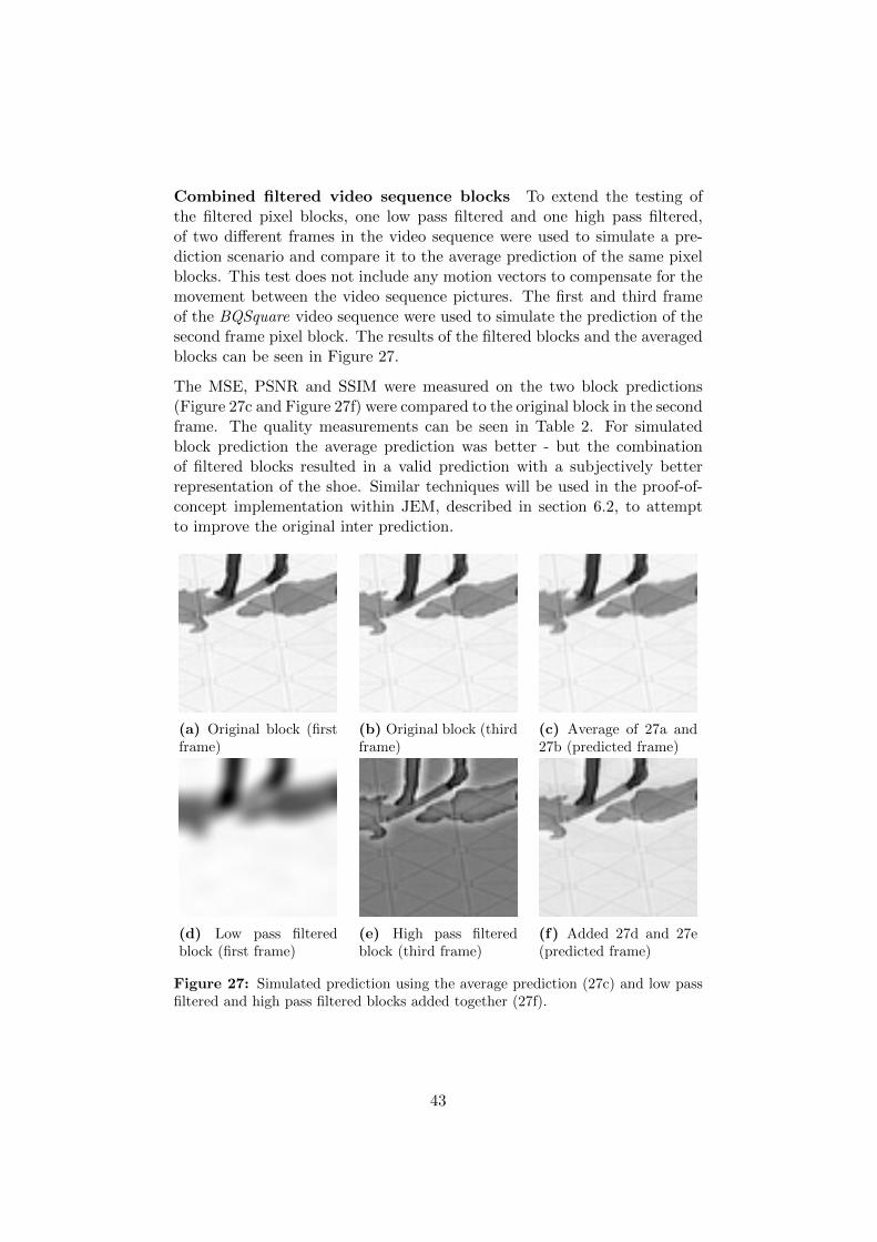
Combined filtered video sequence blocks To extend the testing ofthe filtered pixel blocks, one low pass filtered and one high pass filtered,of two different frames in the video sequence were used to simulate a pre-diction scenario and compare it to the average prediction of the same pixelblocks. This test does not include any motion vectors to compensate for themovement between the video sequence pictures. The first and third frameof the BQSquare video sequence were used to simulate the prediction of thesecond frame pixel block. The results of the filtered blocks and the averagedblocks can be seen in Figure 27.

The MSE, PSNR and SSIM were measured on the two block predictions(Figure 27c and Figure 27f) were compared to the original block in the secondframe. The quality measurements can be seen in Table 2. For simulatedblock prediction the average prediction was better - but the combinationof filtered blocks resulted in a valid prediction with a subjectively betterrepresentation of the shoe. Similar techniques will be used in the proof-of-concept implementation within JEM, described in section 6.2, to attemptto improve the original inter prediction.

(a) Original block (firstframe)

(b) Original block (thirdframe)

(c) Average of 27a and27b (predicted frame)

(d) Low pass filteredblock (first frame)

(e) High pass filteredblock (third frame)

(f) Added 27d and 27e(predicted frame)

Figure 27: Simulated prediction using the average prediction (27c) and low passfiltered and high pass filtered blocks added together (27f).

43

Prediction MSE PSNR SSIM

Low + High 66.806 29.883 dB 0.894

Average 20.731 34.965 dB 0.956

Table 2: Objective measurements of the predicted blocks in Figure 27c and Fig-ure 27f in comparison to the original block of the second frame using MSE, PSNRand SSIM.

6.2 Proof of concept in JEM

The proof of concept implementation in JEM 4.1 has been developed as anextension of the existing uni- and bi-prediction used to evaluate and findthe best prediction mode of each coding unit (CU), i.e. a block of pix-els. The extension aims to improve the prediction and evaluate if filteredblocks has the potential of improving the prediction results, both for uni-or bi-prediction. By allowing for combinations of high pass, low pass andnon-filtered blocks the merged blocks has potential to improve the predic-tion. Bi-prediction is effective, but rate-distortion (RD) costs can limit thecompression quality, hence bi-prediction may be skipped if the RD cost isnot favorable in comparison to uni-prediction.

6.2.1 Filtering in JEM

The filtering performed within JEM 4.1 is either interpolation, deblockingor sample adaptive offset filtering (see section 3.5.4). Instead of developinga separate filtering class, the proof-of-concept implementation has made useof and extended the interpolation filtering class functionality.

The interpolation filtering class, InterpolationFilter, is shared by the en-coder and decoder applications and contains predefined filter coefficients ofinterpolation low pass filters. The filter coefficients are stored in tables (twodimensional arrays) to be used for different types of pixels, e.g. half andquarter pixels. The data array structures are of power of two lengths (2, 4or 8) and the filters of odd or shorter length are padded with zeros. Thereare separate filter tables for the luma and chroma components, lumaFil-ter and chromaFilter (see Listing 3). The luma filters are stored as filterswith up to 8 filter coefficients and the chroma filters have up to 4 filtercoefficients.

The interpolation filtering is performed separately for the horizontal andvertical signals using the filtering functions, filterHor and filterVer (seeListing 3). Internally, both of the filtering functions calls private encapsu-lated functions that perform the actual filtering, i.e. calculating the summa-

44

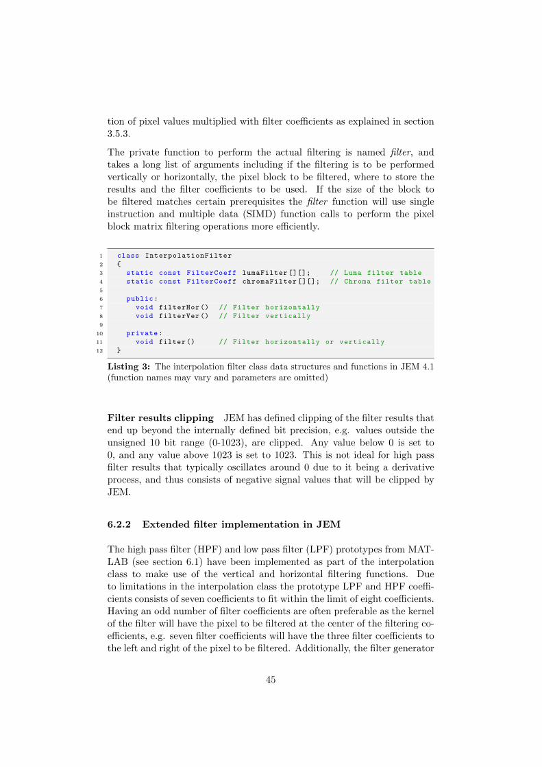
tion of pixel values multiplied with filter coefficients as explained in section3.5.3.

The private function to perform the actual filtering is named filter, andtakes a long list of arguments including if the filtering is to be performedvertically or horizontally, the pixel block to be filtered, where to store theresults and the filter coefficients to be used. If the size of the block tobe filtered matches certain prerequisites the filter function will use singleinstruction and multiple data (SIMD) function calls to perform the pixelblock matrix filtering operations more efficiently.

1 class InterpolationFilter

2 {

3 static const FilterCoeff lumaFilter [][]; // Luma filter table

4 static const FilterCoeff chromaFilter [][]; // Chroma filter table

5

6 public:

7 void filterHor () // Filter horizontally

8 void filterVer () // Filter vertically

9

10 private:

11 void filter () // Filter horizontally or vertically

12 }

Listing 3: The interpolation filter class data structures and functions in JEM 4.1(function names may vary and parameters are omitted)

Filter results clipping JEM has defined clipping of the filter results thatend up beyond the internally defined bit precision, e.g. values outside theunsigned 10 bit range (0-1023), are clipped. Any value below 0 is set to0, and any value above 1023 is set to 1023. This is not ideal for high passfilter results that typically oscillates around 0 due to it being a derivativeprocess, and thus consists of negative signal values that will be clipped byJEM.

6.2.2 Extended filter implementation in JEM

The high pass filter (HPF) and low pass filter (LPF) prototypes from MAT-LAB (see section 6.1) have been implemented as part of the interpolationclass to make use of the vertical and horizontal filtering functions. Dueto limitations in the interpolation class the prototype LPF and HPF coeffi-cients consists of seven coefficients to fit within the limit of eight coefficients.Having an odd number of filter coefficients are often preferable as the kernelof the filter will have the pixel to be filtered at the center of the filtering co-efficients, e.g. seven filter coefficients will have the three filter coefficients tothe left and right of the pixel to be filtered. Additionally, the filter generator

45

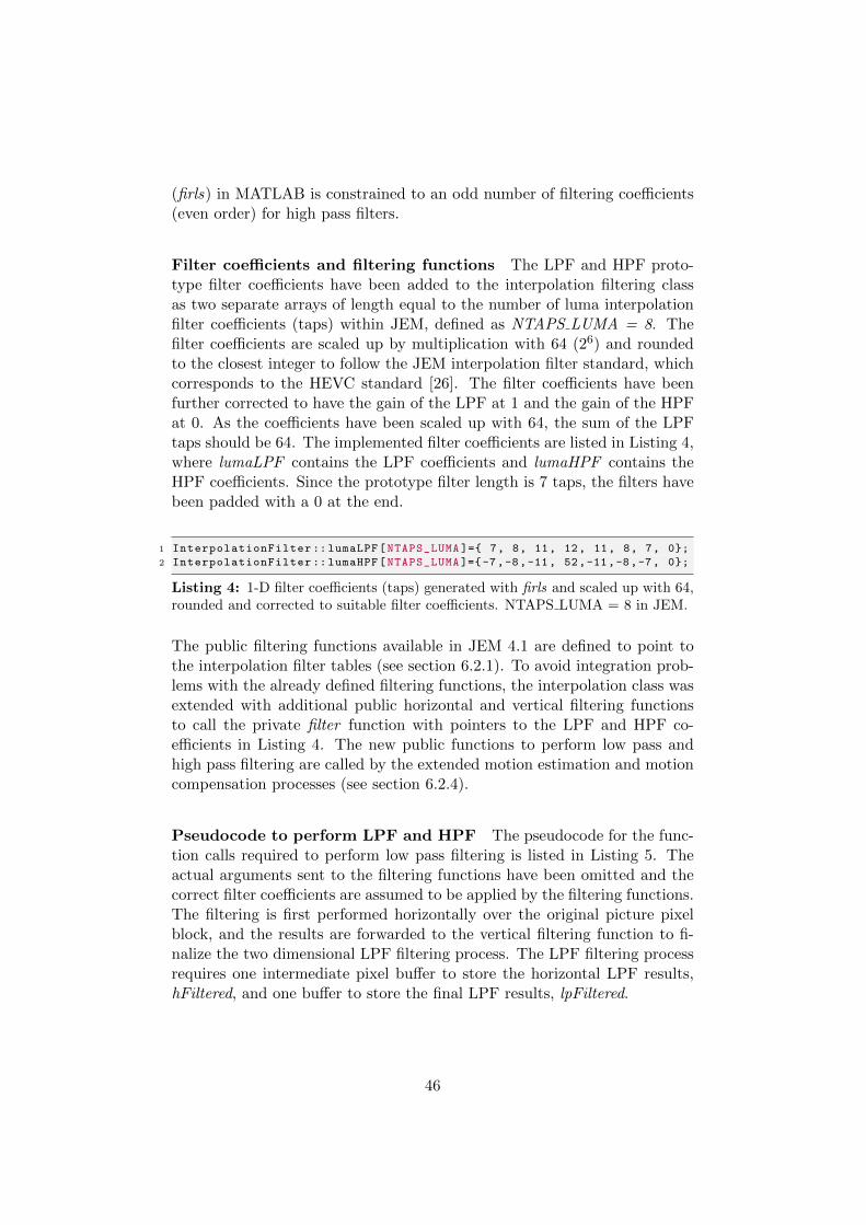
(firls) in MATLAB is constrained to an odd number of filtering coefficients(even order) for high pass filters.

Filter coefficients and filtering functions The LPF and HPF proto-type filter coefficients have been added to the interpolation filtering classas two separate arrays of length equal to the number of luma interpolationfilter coefficients (taps) within JEM, defined as NTAPS LUMA = 8. Thefilter coefficients are scaled up by multiplication with 64 (26) and roundedto the closest integer to follow the JEM interpolation filter standard, whichcorresponds to the HEVC standard [26]. The filter coefficients have beenfurther corrected to have the gain of the LPF at 1 and the gain of the HPFat 0. As the coefficients have been scaled up with 64, the sum of the LPFtaps should be 64. The implemented filter coefficients are listed in Listing 4,where lumaLPF contains the LPF coefficients and lumaHPF contains theHPF coefficients. Since the prototype filter length is 7 taps, the filters havebeen padded with a 0 at the end.

1 InterpolationFilter :: lumaLPF[NTAPS_LUMA ]={ 7, 8, 11, 12, 11, 8, 7, 0};

2 InterpolationFilter :: lumaHPF[NTAPS_LUMA ]={-7,-8,-11, 52,-11,-8,-7, 0};

Listing 4: 1-D filter coefficients (taps) generated with firls and scaled up with 64,rounded and corrected to suitable filter coefficients. NTAPS LUMA = 8 in JEM.

The public filtering functions available in JEM 4.1 are defined to point tothe interpolation filter tables (see section 6.2.1). To avoid integration prob-lems with the already defined filtering functions, the interpolation class wasextended with additional public horizontal and vertical filtering functionsto call the private filter function with pointers to the LPF and HPF co-efficients in Listing 4. The new public functions to perform low pass andhigh pass filtering are called by the extended motion estimation and motioncompensation processes (see section 6.2.4).

Pseudocode to perform LPF and HPF The pseudocode for the func-tion calls required to perform low pass filtering is listed in Listing 5. Theactual arguments sent to the filtering functions have been omitted and thecorrect filter coefficients are assumed to be applied by the filtering functions.The filtering is first performed horizontally over the original picture pixelblock, and the results are forwarded to the vertical filtering function to fi-nalize the two dimensional LPF filtering process. The LPF filtering processrequires one intermediate pixel buffer to store the horizontal LPF results,hFiltered, and one buffer to store the final LPF results, lpFiltered.

46

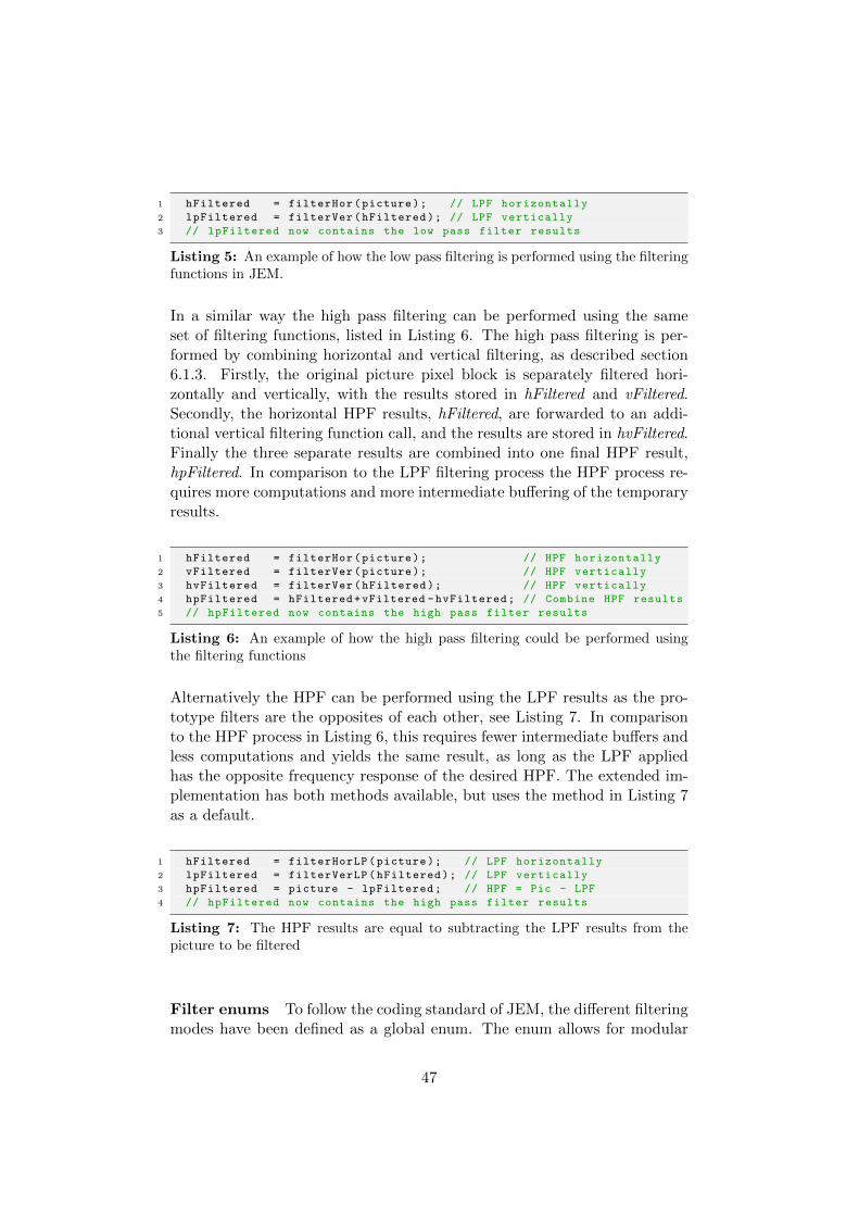
1 hFiltered = filterHor(picture); // LPF horizontally

2 lpFiltered = filterVer(hFiltered); // LPF vertically

3 // lpFiltered now contains the low pass filter results

Listing 5: An example of how the low pass filtering is performed using the filteringfunctions in JEM.

In a similar way the high pass filtering can be performed using the sameset of filtering functions, listed in Listing 6. The high pass filtering is per-formed by combining horizontal and vertical filtering, as described section6.1.3. Firstly, the original picture pixel block is separately filtered hori-zontally and vertically, with the results stored in hFiltered and vFiltered.Secondly, the horizontal HPF results, hFiltered, are forwarded to an addi-tional vertical filtering function call, and the results are stored in hvFiltered.Finally the three separate results are combined into one final HPF result,hpFiltered. In comparison to the LPF filtering process the HPF process re-quires more computations and more intermediate buffering of the temporaryresults.

1 hFiltered = filterHor(picture); // HPF horizontally

2 vFiltered = filterVer(picture); // HPF vertically

3 hvFiltered = filterVer(hFiltered); // HPF vertically

4 hpFiltered = hFiltered+vFiltered -hvFiltered; // Combine HPF results

5 // hpFiltered now contains the high pass filter results

Listing 6: An example of how the high pass filtering could be performed usingthe filtering functions

Alternatively the HPF can be performed using the LPF results as the pro-totype filters are the opposites of each other, see Listing 7. In comparisonto the HPF process in Listing 6, this requires fewer intermediate buffers andless computations and yields the same result, as long as the LPF appliedhas the opposite frequency response of the desired HPF. The extended im-plementation has both methods available, but uses the method in Listing 7as a default.

1 hFiltered = filterHorLP(picture); // LPF horizontally

2 lpFiltered = filterVerLP(hFiltered); // LPF vertically

3 hpFiltered = picture - lpFiltered; // HPF = Pic - LPF

4 // hpFiltered now contains the high pass filter results

Listing 7: The HPF results are equal to subtracting the LPF results from thepicture to be filtered

Filter enums To follow the coding standard of JEM, the different filteringmodes have been defined as a global enum. The enum allows for modular

47

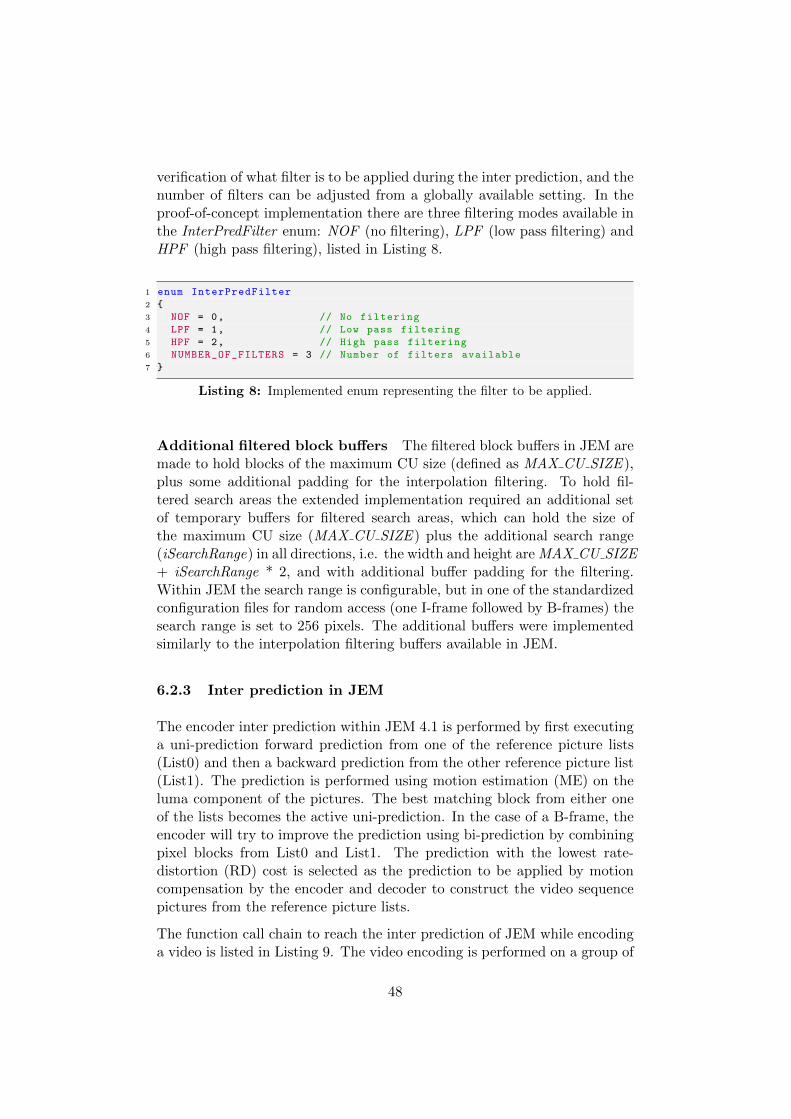
verification of what filter is to be applied during the inter prediction, and thenumber of filters can be adjusted from a globally available setting. In theproof-of-concept implementation there are three filtering modes available inthe InterPredFilter enum: NOF (no filtering), LPF (low pass filtering) andHPF (high pass filtering), listed in Listing 8.

1 enum InterPredFilter

2 {

3 NOF = 0, // No filtering

4 LPF = 1, // Low pass filtering

5 HPF = 2, // High pass filtering

6 NUMBER_OF_FILTERS = 3 // Number of filters available

7 }

Listing 8: Implemented enum representing the filter to be applied.

Additional filtered block buffers The filtered block buffers in JEM aremade to hold blocks of the maximum CU size (defined as MAX CU SIZE ),plus some additional padding for the interpolation filtering. To hold fil-tered search areas the extended implementation required an additional setof temporary buffers for filtered search areas, which can hold the size ofthe maximum CU size (MAX CU SIZE ) plus the additional search range(iSearchRange) in all directions, i.e. the width and height are MAX CU SIZE+ iSearchRange * 2, and with additional buffer padding for the filtering.Within JEM the search range is configurable, but in one of the standardizedconfiguration files for random access (one I-frame followed by B-frames) thesearch range is set to 256 pixels. The additional buffers were implementedsimilarly to the interpolation filtering buffers available in JEM.

6.2.3 Inter prediction in JEM

The encoder inter prediction within JEM 4.1 is performed by first executinga uni-prediction forward prediction from one of the reference picture lists(List0) and then a backward prediction from the other reference picture list(List1). The prediction is performed using motion estimation (ME) on theluma component of the pictures. The best matching block from either oneof the lists becomes the active uni-prediction. In the case of a B-frame, theencoder will try to improve the prediction using bi-prediction by combiningpixel blocks from List0 and List1. The prediction with the lowest rate-distortion (RD) cost is selected as the prediction to be applied by motioncompensation by the encoder and decoder to construct the video sequencepictures from the reference picture lists.

The function call chain to reach the inter prediction of JEM while encodinga video is listed in Listing 9. The video encoding is performed on a group of

48

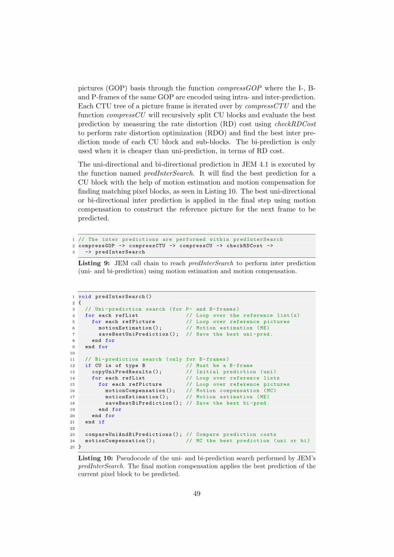
pictures (GOP) basis through the function compressGOP where the I-, B-and P-frames of the same GOP are encoded using intra- and inter-prediction.Each CTU tree of a picture frame is iterated over by compressCTU and thefunction compressCU will recursively split CU blocks and evaluate the bestprediction by measuring the rate distortion (RD) cost using checkRDCostto perform rate distortion optimization (RDO) and find the best inter pre-diction mode of each CU block and sub-blocks. The bi-prediction is onlyused when it is cheaper than uni-prediction, in terms of RD cost.

The uni-directional and bi-directional prediction in JEM 4.1 is executed bythe function named predInterSearch. It will find the best prediction for aCU block with the help of motion estimation and motion compensation forfinding matching pixel blocks, as seen in Listing 10. The best uni-directionalor bi-directional inter prediction is applied in the final step using motioncompensation to construct the reference picture for the next frame to bepredicted.

1 // The inter predictions are performed within predInterSearch

2 compressGOP -> compressCTU -> compressCU -> checkRDCost ->

3 -> predInterSearch

Listing 9: JEM call chain to reach predInterSearch to perform inter prediction(uni- and bi-prediction) using motion estimation and motion compensation.

1 void predInterSearch ()

2 {

3 // Uni -prediction search (for P- and B-frames)

4 for each refList // Loop over the reference list(s)

5 for each refPicture // Loop over reference pictures

6 motionEstimation (); // Motion estimation (ME)

7 saveBestUniPrediction (); // Save the best uni -pred.

8 end for

9 end for

10

11 // Bi -prediction search (only for B-frames)

12 if CU is of type B // Must be a B-frame

13 copyUniPredResults (); // Initial prediction (uni)

14 for each refList // Loop over reference lists

15 for each refPicture // Loop over reference pictures

16 motionCompensation (); // Motion compensation (MC)

17 motionEstimation (); // Motion estimation (ME)

18 saveBestBiPrediction (); // Save the best bi -pred.

19 end for

20 end for

21 end if

22

23 compareUniAndBiPredictions (); // Compare prediction costs

24 motionCompensation (); // MC the best prediction (uni or bi)

25 }

Listing 10: Pseudocode of the uni- and bi-prediction search performed by JEM’spredInterSearch. The final motion compensation applies the best prediction of thecurrent pixel block to be predicted.

49

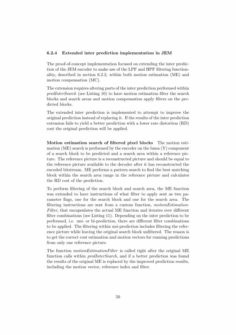
6.2.4 Extended inter prediction implementation in JEM

The proof-of-concept implementation focused on extending the inter predic-tion of the JEM encoder to make use of the LPF and HPF filtering function-ality, described in section 6.2.2, within both motion estimation (ME) andmotion compensation (MC).

The extension requires altering parts of the inter prediction performed withinpredInterSearch (see Listing 10) to have motion estimation filter the searchblocks and search areas and motion compensation apply filters on the pre-dicted blocks.

The extended inter prediction is implemented to attempt to improve theoriginal prediction instead of replacing it. If the results of the inter predictionextension fails to yield a better prediction with a lower rate distortion (RD)cost the original prediction will be applied.

Motion estimation search of filtered pixel blocks The motion esti-mation (ME) search is performed by the encoder on the luma (Y) componentof a search block to be predicted and a search area within a reference pic-ture. The reference picture is a reconstructed picture and should be equal tothe reference picture available to the decoder after it has reconstructed theencoded bitstream. ME performs a pattern search to find the best matchingblock within the search area range in the reference picture and calculatesthe RD cost of the prediction.

To perform filtering of the search block and search area, the ME functionwas extended to have instructions of what filter to apply sent as two pa-rameter flags, one for the search block and one for the search area. Thefiltering instructions are sent from a custom function, motionEstimation-Filter, that encapsulates the actual ME function and iterates over differentfilter combinations (see Listing 11). Depending on the inter prediction to beperformed, i.e. uni- or bi-prediction, there are different filter combinationsto be applied. The filtering within uni-prediction includes filtering the refer-ence picture while leaving the original search block unfiltered. The reason isto get the correct cost estimation and motion vectors for running predictionsfrom only one reference picture.

The function motionEstimationFilter is called right after the original MEfunction calls within predInterSearch, and if a better prediction was foundthe results of the original ME is replaced by the improved prediction results,including the motion vector, reference index and filter.

50

1 // Iterates over filters and calls ME with filtering instructions

2 void motionEstimationFilter ()

3 {

4 for each filter

5 filterBlock = biPred ? filter : NOF; // Block filter

6 filterArea = filter; // Search area filter

7 motionEstimation(filterBlock , filterArea);// ME filter

8

9 if(cost < bestCost) // RD cost from ME

10 saveBestPrediction (); // Save best prediction

11 end for

12 }

Listing 11: The motion estimation is encapsulated in motionEstimationFilter toiterate over different filter combinations, depending on uni- or bi-prediction.

The uni-prediction is responsible for performing both the regular uni-prediction(see Figure 28a) and the pre-bi-prediction (see Figure 28b) where both thesearch area and the search block are filtered to find the best matching blocksof each filtered component, e.g. a low pass filtered search block is motionestimated on a low pass filtered search area. The cost of such a motionestimation does not represent a real prediction of the original block, buta prediction of a filtered original block, hence those costs are not valid foruni-prediction. The reason for having uni-prediction perform the pre-bi-prediction ME filtering is that the bi-prediction loop in predInterSearch willapply the initial motion compensation based on the uni-prediction results,and then run the bi-predictive motion estimation, with the motion compen-sated block weighed in as one of the two predictions of bi-prediction.

(a) Uni-prediction filtering. (b) Pre-bi-prediction filtering.

Figure 28: Uni-prediction performs motion estimation on the block to be esti-mated, with and without using filtering, depending on the mode.

The bi-prediction loop has been extended similarly to how uni-predictioncalls motionEstimationFilter to try and improve the uni-prediction. A sep-arate bi-prediction function, improveBiPrediction (see Listing 12), appliesthe pre-bi-prediction results from the uni-prediction loop using motion com-pensation and then calls motionEstimationFilter with the bi-prediction flagset to true to calculate the costs of the bi-prediction using combinations ofnon-filtered and filtered block predictions (see Figure 29). The bi-prediction

51

motion estimation will subtract the motion compensated block from theblock to be predicted and then the motion estimation will search for thebest matching block of the remainder, hence it finds the best matchingblock combination for the block to be predicted.

1 // Iterates over filters and calls MC with filtering instructions

2 void improveBiPrediction ()

3 {

4 for each ref // Loop over reference pics

5 for each filter // Loop over filters

6 getPrediction(ref); // Pre -bi-pred MV and filter

7 motionCompensation(ref , mv, filter);// MC: Apply pre -bi -pred

8 motionEstimationFilter(biPred); // ME: Find matching block

9

10 if (cost < bestCostBi) // RD cost from ME

11 saveBestPrediction (); // Save best prediction

12 end for

13 end for

14 }

Listing 12: An encapsulating function to apply the filtered results from the pre-bi-prediction using MC and running the the filtering ME to find the best matchingblocks.

Figure 29: Bi-prediction filtering. The block to be predicted is subtracted bythe motion compensated block, resulting in a remainder that is searched for usingmotion estimation and filtering of the search area.

The two functions, motionEstimationFilter and improveBiPrediction, havebeen implemented into the inter prediction function of JEM, predInterSearch(see lines 7 and 18 in Listing 13). The behavior of the inter prediction inJEM is retained, and the extensions will attempt to improve the originalpredictions. If an improved prediction is found it will replace the originalprediction to be applied in the final motion compensation call of predInter-Search (see line 25 in Listing 13).

52

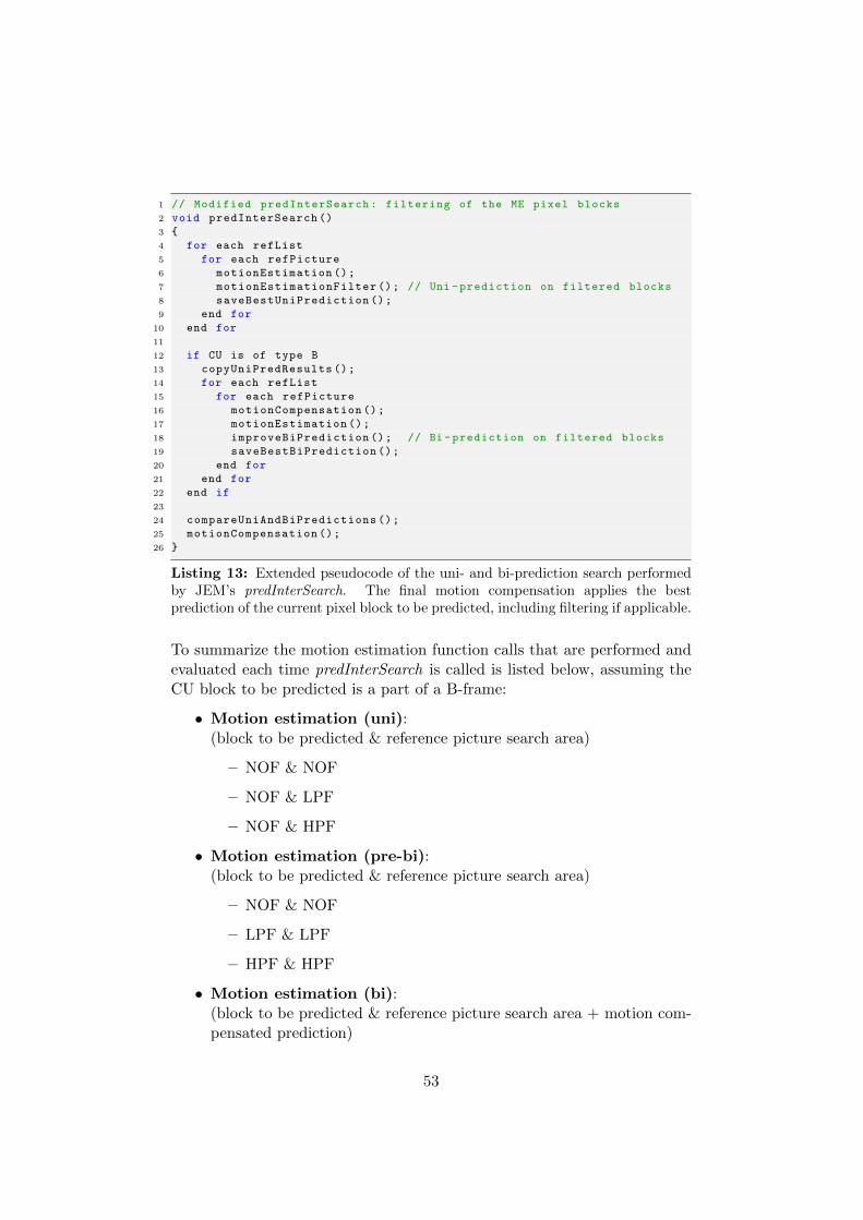
1 // Modified predInterSearch: filtering of the ME pixel blocks

2 void predInterSearch ()

3 {

4 for each refList

5 for each refPicture

6 motionEstimation ();

7 motionEstimationFilter (); // Uni -prediction on filtered blocks

8 saveBestUniPrediction ();

9 end for

10 end for

11

12 if CU is of type B

13 copyUniPredResults ();

14 for each refList

15 for each refPicture

16 motionCompensation ();

17 motionEstimation ();

18 improveBiPrediction (); // Bi-prediction on filtered blocks

19 saveBestBiPrediction ();

20 end for

21 end for

22 end if

23

24 compareUniAndBiPredictions ();

25 motionCompensation ();

26 }

Listing 13: Extended pseudocode of the uni- and bi-prediction search performedby JEM’s predInterSearch. The final motion compensation applies the bestprediction of the current pixel block to be predicted, including filtering if applicable.

To summarize the motion estimation function calls that are performed andevaluated each time predInterSearch is called is listed below, assuming theCU block to be predicted is a part of a B-frame:

• Motion estimation (uni):(block to be predicted & reference picture search area)

– NOF & NOF

– NOF & LPF

– NOF & HPF

• Motion estimation (pre-bi):(block to be predicted & reference picture search area)

– NOF & NOF

– LPF & LPF

– HPF & HPF

• Motion estimation (bi):(block to be predicted & reference picture search area + motion com-pensated prediction)

53

– NOF & NOF + MC(NOF/LPF/HPF)

– NOF & LPF + MC(NOF/LPF/HPF)

– NOF & HPF + MC(NOF/LPF/HPF)

As motion estimation search is a part of both uni- and bi-prediction, thebest prediction of those two will become the final prediction to be applied inthe final motion compensation of predInterSearch. In uni-prediction the bestblock, either filtered or not filtered, from both of the reference picture listsare saved as separate prediction candidates, and in bi-prediction the bestcombination of blocks, filtered or not filtered, will become the final predictioncandidate. For example, the bi-prediction may include a combination of aLPF block and a HPF block or a NOF block and a LPF block, dependingon what combination yielded the lowest RD-cost.

The extended inter prediction results in more computations, as motion es-timation is performed several times for each CU, adding to the alreadyexisting computational complexity of the motion estimation of predInter-Search. Additionally, several filtering operations are performed each timemotion estimation is called, including LPF, HPF and interpolation filtering,on the CU block to be predicted and the search area. The encoding timesare therefore expected to increase significantly.

Limited motion estimation filtering A a reference picture may achievebenefits from filtering, but as the filtering will change, the data containedwithin the picture it could potentially lead to losses in the pictures thatuse the filtered picture as a reference. The picture referencing structure istypically represented hierarchically as a group of pictures (GOP) (see sec-tion 3.4.4). The hierarchical structure of the GOP divides the frames intotemporal layers based on the order of which the pictures are encoded anddecoded, as seen in Figure 30. Pictures at the lowest temporal layer (layer0) can be used as a reference, directly or indirectly, by the temporal layersabove, while the pictures at the top layer (layer 4) will not be used as refer-ence pictures. Filtering data within the GOP has the potential of yieldingbenefits for some pictures, while it could potentially result in worse resultfor other pictures as the data within the hierarchical referencing structurewill be altered in comparison to not having filtering enabled at all.

54

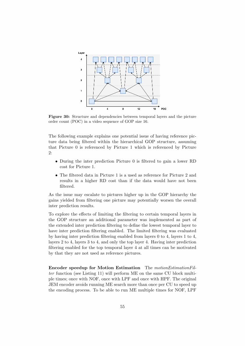
Figure 30: Structure and dependencies between temporal layers and the pictureorder count (POC) in a video sequence of GOP size 16.

The following example explains one potential issue of having reference pic-ture data being filtered within the hierarchical GOP structure, assumingthat Picture 0 is referenced by Picture 1 which is referenced by Picture2:

• During the inter prediction Picture 0 is filtered to gain a lower RDcost for Picture 1.

• The filtered data in Picture 1 is a used as reference for Picture 2 andresults in a higher RD cost than if the data would have not beenfiltered.

As the issue may escalate to pictures higher up in the GOP hierarchy thegains yielded from filtering one picture may potentially worsen the overallinter prediction results.

To explore the effects of limiting the filtering to certain temporal layers inthe GOP structure an additional parameter was implemented as part ofthe extended inter prediction filtering to define the lowest temporal layer tohave inter prediction filtering enabled. The limited filtering was evaluatedby having inter prediction filtering enabled from layers 0 to 4, layers 1 to 4,layers 2 to 4, layers 3 to 4, and only the top layer 4. Having inter predictionfiltering enabled for the top temporal layer 4 at all times can be motivatedby that they are not used as reference pictures.

Encoder speedup for Motion Estimation The motionEstimationFil-ter function (see Listing 11) will perform ME on the same CU block multi-ple times; once with NOF, once with LPF and once with HPF. The originalJEM encoder avoids running ME search more than once per CU to speed upthe encoding process. To be able to run ME multiple times for NOF, LPF

55

and HPF the JEM speedup implementation has been extended to enablethe encoder to function with multiple ME searches. The original encoderspeedup includes multidimensional arrays within each CU to store the esti-mated motion vector from previous ME searches. The arrays were extendedwith two additional dimensions, one for the filter parameter of the searchblock and one for the search area. For example, the results from having aLPF search area and a NOF search block is kept separate from the resultsof a LPF search area and a LPF search block.5 The encoder speedup isonly active for the unidirectional ME search in JEM and does not affect thebidirectional ME search.

Motion compensation filtering The best results of the motion estima-tions, including uni- and bi-prediction, have the potential to be used forthe final prediction and are applied by motion compensation. If the bestprediction block was found to benefit from filtering in ME, the same filteris applied during the MC process. For MC to apply the correct predictionof each pixel block, the best estimation, including what reference pictureto use, what motion vector to apply and if the block should be filtered, isstored in each coding unit (CU). The filter flag is stored as part of the CUobject similarly to how the motion vectors and reference picture indices arestored within CUs in JEM. The motion compensation function reads theCU parameters and applies the motion vector and filter specified.

The proof-of-concept implementation was delimited to the JEM video en-coder, and does not include the CU filtering instructions as part of thebitstream to be sent to the decoder for reconstruction. Although, as JEMis a hybrid video coder, the encoder will reconstruct the compressed videosequence similarly to how the decoder would do it, which produces validmeasurable video sequence results. The encoder and decoder share somecommon classes, including the CU class that holds the filter parameters andprediction class that contains the MC function. Therefore, if the CU filterparameters are encoded into the compressed bitstream, the decoder onlyneeds to be adjusted to read the additional bitstream parameters for themto be applied during the reconstruction of the video sequence.

56

7 Results

The results presented in this section are based on the proof-of-concept im-plementation (see section 6.2) within the JEM framework evaluated on a setof video sequences commonly used to compare video coders and video cod-ing methods. The video sequences are divided into different classes listed inTable 3 depending on their content and resolution [10][p. 94]. Due to timelimitations the results are based on the fast test video sequences that con-tains a cropped portion of the original videos, except for class D. The framerates differ for each video sequence and has not been included here.

Video class Resolution Cropped

Class A1 2560x1600 1024x512Class A2 2560x1600 512x256Class B 1920x1080 416x320Class C 832x480 416x320Class D 416x240 416x240

Table 3: Video classes and their corresponding resolutions.

Additionally, the testing conditions have been limited to the common testingcondition (CTC) random access (RA), defined by JCT-VC, which representsbroadcast and streaming applications with high compression performance[10][p. 93]. As the project focuses on the filtering of bidirectional predictionblocks the configuration of the JEM encoder has been based on the stan-dardized JVET Main 10 profile random access configuration, which has aGOP size of 16 structured as in Figure 30. The standardized JEM encod-ing configuration file is available in the JVET JEM 4.1 software repository[7].

To run the test sequences with the modified JEM encoder more efficiently,Ericsson Research provided automated scripts to run the encoder with eachvideo sequence as a job on their computer cluster. The results are automat-ically compiled into a Microsoft Excel document with predefined macros tocalculate and presents the results, including PSNR, SSIM, BD-rate and theelapsed time, in comparison to a reference encoder, which in this case is theoriginal JEM 4.1 encoder. The number of frames of each video sequence torun the encoder on has been limited due to time constraints.

7.1 Objective BD-rate results

The results from the objective BD-rate evaluations are presented below,including one short encoding test of the first 17 frames and a longer test of

57

50 frames. The BD-rate results are based on measurements of PSNR andSSIM over the three channels in the YUV color space, i.e. luminosity (Y),chromatic blue (U) and chromatic red (V) (see section 3.1.2)

7.1.1 Overall results

The overall results includes the results from all the video classes. The firsttest was limited to encode the first 17 frames of each video sequence to covera whole GOP, one I-frame and 16 B-frames. To compare the filtering overseveral temporal layers, separate encodings were performed for filtering onlylayer 4 (TL4), layer 3 and up (TL3), layer 2 and up (TL2), layer 1 and up(TL1), and finally layer 0 and up (TL0) which includes all the B-framesof the GOP. The overall results are compiled into Figure 31. The detailedresults can be found in appendix A.1.

(a) 17 frames PSNR BD-rate (b) 17 frames SSIM BD-rate

Figure 31: Overall PSNR and SSIM BD-rate results for the first 17 frames of thevideo sequence test set.

(a) 50 frames PSNR BD-rate (b) 50 frames SSIM BD-rate

Figure 32: Overall PSNR and SSIM BD-rate results for the first 50 frames of thevideo sequence test set.

58

7.1.2 Per video class results

The results for video classes A1 and A2 tended to gain more from the fil-tering, while the video classes B, C and D had varying results, often withBD-rate losses. The PSNR and SSIM BD-rate results per video class fromthe encoding test of the first 17 frames can be seen in Figure 33, and theencoding test of the first 50 frames can be seen in Figure 34. The detailedresults per video sequence class can be found in appendix A.1.

Figure 33: PSNR (top) and SSIM (bottom) BD-rate results per video sequenceclass for the first 17 frames of the video sequence.

Figure 34: PSNR (top) and SSIM (bottom) BD-rate results per video sequenceclass for the first 50 frames of the video sequence.

59

Per video sequence results The results of each individual video se-quences varied, even if they were part of the same video class. One of thevideo sequences in video class A2, RollerCoaster, had the most gains in theluma (Y) channel, and consistent PSNR BD-rate gains in all YUV chan-nels (see Figure 35). The detailed results for each video sequence have beenincluded in appendix A.2.

(a) 50 frames PSNR BD-rate (b) 50 frames SSIM BD-rate

Figure 35: Video sequence RollerCoaster PSNR and SSIM BD-rate results forthe first 50 frames.

7.1.3 Computational complexity

To further evaluate the proof-of-concept implementation the overall timesfor encoding are compared with the original JEM encoder in Figure 36. Theencoding times gives an overview of the added computational complexity,caused by the additional motion estimation and motion compensation of theproof-of-concept implementation.

Figure 36: Computational complexity per temporal layer filtered in comparisonto the original JEM encoder baseline.

60

7.2 Subjective quality with examples

The subjective quality differences of the reconstructed video sequences aresmall and hard to notice unless you directly compare individual frames be-tween the reconstructed video sequences. Even then it is hard to say whichone of the frames look subjectively better. Some of the more noticeabledifferences can be seen in Figure 37, Figure 38 and Figure 39, althoughthe differences are not noticeable unless you compare the individual videosequence pictures side by side.

(a) Frame 5 from RollerCoaster(Class A1)

(b) Original frame 5 cropped to thearea of interest.

(c) Original JEM encoding recon-struction of the area of interest

(d) Extended JEM encoding recon-struction of the area of interest

Figure 37: An example of encoding differences between the original and extendedJEM encoder. The extended JEM encoder retains the details of the railing behindthe people in the background.

61

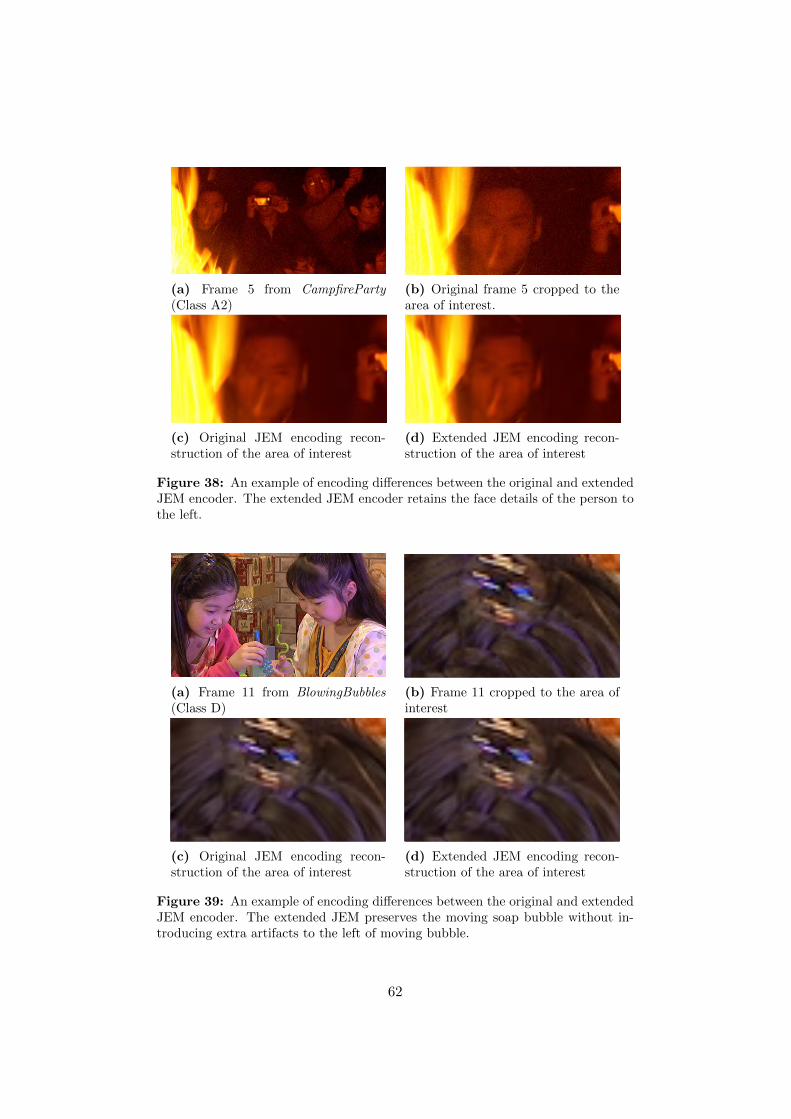
(a) Frame 5 from CampfireParty(Class A2)

(b) Original frame 5 cropped to thearea of interest.

(c) Original JEM encoding recon-struction of the area of interest

(d) Extended JEM encoding recon-struction of the area of interest

Figure 38: An example of encoding differences between the original and extendedJEM encoder. The extended JEM encoder retains the face details of the person tothe left.

(a) Frame 11 from BlowingBubbles(Class D)

(b) Frame 11 cropped to the area ofinterest

(c) Original JEM encoding recon-struction of the area of interest

(d) Extended JEM encoding recon-struction of the area of interest

Figure 39: An example of encoding differences between the original and extendedJEM encoder. The extended JEM preserves the moving soap bubble without in-troducing extra artifacts to the left of moving bubble.

62

8 Conclusion and discussion

The purpose of this thesis was to evaluate low pass and high pass filteringwithin the inter prediction of the Joint Exploration Model (JEM) to answerthe problem statement: can the video picture data be reshaped for betterprediction and compression?. The initial research of related work pointedto that, even though video coding and compression includes several filter-ing techniques, similar methods have not previously been implemented andevaluated. A proof-of-concept implementation was therefore required.

The proof-of-concept implementation with low pass and high pass filteringwithin the inter prediction of JEM resulted in varying results between in-dividual video sequences and video classes, which is to be expected. Theunexpected results came from the video sequences that resulted in overalllosses in all luminosity and chroma channels and the ones that had signifi-cant losses in only the luminosity channel. The implementation applies thefiltering when the rate-distortion (RD) cost is calculated to be lower, hencethe results are expected to result in gains, especially when only the picturesin the top temporal layer, layer 4, is filtered as they are not used as refer-ences for any other pictures in the encoding sequence. But the filtering ofthe top temporal layer did actually affect other layers through other pro-cesses of the JEM encoder, one being the adaptive loop filter (ALF) whichadapts its filtering from all previously encoded pictures.

JEM is a large software framework maintained by video coding experts, andimplementing relatively small extensions requires a good understanding ofvideo coding on a conceptual level and how JEM performs the encoding onthe program code level. Debugging JEM is time consuming and the codebase contains minimal documentation. Since JEM is under development itcontains several experimental macros to encapsulate code blocks, which isgood for testing implementation suggestions but hinders readability.

Initially it was expected that the layer to gain benefits from the inter pre-diction filtering was the luminosity (Y) channel, and not the chromatic blue(U) nor the chromatic red (V), due to inter prediction filtering only beingapplied on the Y channel. The inter prediction filtering is likely to find mo-tion vectors that differ from the non-filtered inter prediction, and since themotion vectors are applied on all YUV channels it will result in differences inthe chroma channels as well. As the total RD cost is calculated over all threeYUV channels, the result benefits in the chroma channels tend to outweighthe losses in the luma channel, with exceptions for the lower resolution videoclasses B, C, and D.

The results are limited to the performances of the low pass filter (LPF) andhigh pass filter (HPF) prototypes. Other filters, with different characteristics

63

and cutoff frequencies, could potentially improve the results further. Thecutoff frequencies used in this project, at 0.2 normalized frequency, wasbased on the cutoff frequencies of the interpolation filters in AVC and HEVC,at 0.5 normalized frequency, and aimed to split the remaining frequencyspectrum in close to half. Additionally the cutoff frequency at 0.2 wasselected due to the subjectively distinct blurred results when using the LPFand the edge detecting results of the HPF. If more time would have beenavailable it could have been interesting to compare several different typesof filters and filter combinations. Although missing from the results, theproof-of-concept implementation seemed to favor the LPF for several of thevideo sequences, while the HPF was not used all that much. One reasoncould be the undesired signal clipping of the resulting negative pixel values,causing pixel data to be lost. The extended implementation of JEM includeda function to log the filtering decisions of the final motion compensationdecision of the inter prediction function, but due to time limitations therewas not enough data gathered to be presented in the result section.

The encoding times are highly affected by the extra filtering, additionalmotion estimation for both uni- and bi-prediction and motion compensationswithin bi-prediction. The additional computational complexity is increasedfor each temporal layer filtered and is not suitable unless the additionalencoding times are of no issue. The motion estimation filtering processcould potentially be optimized by limiting it to certain sizes of CU blocks,or only having the LPF and HPF filters applied on the blocks found by theregular motion estimation.

In conclusion, connecting back to the problem statements, it is possible toreshape the picture data of a video sequence using low pass and high passfilters to achieve better inter predictions and compression. Although theresults are varying, the proof-of-concept implementation managed to showthat there are benefits to be gained in some video sequences, especially invideo classes A1 and A2, from having the luma channel be filtered for themotion estimation and motion compensation. There are still implementationimprovements to be addressed that potentially could improve the results,which are discussed as future work in section 9.

64

9 Future work

As discussed in the conclusion and discussion (see section 8), the proof-of-concept implementation has the potential to be improved. Some of the im-provements were attempted to be implemented, but time limitations forcedthem to be discarded, so that the time consuming tests of the proof-of-concept could yield valid results for evaluation.

One of the issues that was attempted to be addressed is the clipping of neg-ative pixel values as a result of the high pass filtered signal. Adjustmentswere made to offset the filtered pixel values with the average luma pixel value(DC) of the picture in which the block to be filtered originated from. Theoffset will retain the HPF signal, but requires adjustments within motionestimation and motion compensation to remove the offset and restore theoriginal HPF signal to be used in combination with NOF, LPF and otherHPF pixel blocks. The HPF offset also needs to be addressed within theinterpolation filtering where pixel value clipping is applied, including frac-tional pixel pattern search in the motion estimation and the creation of themotion compensated blocks.

For the bi-prediction to correctly take the filtered blocks into consideration,it needs to be able to subtract the already filtered motion compensated blockfrom the block to be predicted. In the current implementation of JEM 4.1,the bi-prediction is based on the average weighted prediction of two blocks,hence within motion estimation the original block to be predicted is sub-tracted by half the signal amplitude of the applied filtered motion compen-sated block, and then motion estimation will search for the best matchingblock of the remaining signal. The modification requires subtracting theblock to be predicted with the full signal amplitude of the filtered motioncompensated block to find the best matching filtered block combination, e.g.LPF+HPF or NOF+HPF, without the averaging of the filtered blocks. Theaveraging should be retained for the chroma channels as they are not splitinto separate filtered components.

In similar to how the motion estimation needs to be modified to retain theamplitude of the LPF and HPF signals, the same is true for the motion com-pensation, which applies the filtering and combines the bi-prediction blocksusing weighted prediction based on the weighted average. The weightedprediction within motion compensation must be able to weigh the filteredluma components equally at their full amplitude, e.g. LPF+HPF insteadof LPF/2 + HPF/2, while having the original weighted prediction behaviorfor the chroma components.

Finally, one JEM extension that was discussed, but discarded early in theproject due to time limitations, was the signaling of the NOF, LPF and HPF

65

filtering flags within the bitstream sent to the decoder. That is the only wayfor the decoder to reconstruct the same representation of the video sequenceas the encoder with the filtering extension enabled. The filter signalingwould require a few extra bits per CU and would have to be included withinthe RD cost calculations for the costs to be fully representable of the bitraterequired for the encoding.

66

References

[1] The Zettabyte Era — Trends and Analysis. http://www.

cisco.com/c/en/us/solutions/collateral/service-provider/

visual-networking-index-vni/vni-hyperconnectivity-wp.html.[Online: 2017-02-10].

[2] Cisco Visual Networking Index: Global Mobile Data Traf-fic Forecast Update, 2016–2021 White Paper. http://www.

cisco.com/c/en/us/solutions/collateral/service-provider/

visual-networking-index-vni/mobile-white-paper-c11-520862.

html. [Online: 2017-02-10].

[3] T. Wiegand, G.J. Sullivan, G. Bjontegaard, and A. Luthra. Overview ofthe H.264/AVC video coding standard. IEEE Transactions on Circuitsand Systems for Video Technology, 13(7):560–576, July 2003.

[4] Gary J. Sullivan, Jens-Rainer Ohm, Woo-Jin Han, and Thomas Wie-gand. Overview of the High Efficiency Video Coding (HEVC) Stan-dard. IEEE Transactions on Circuits and Systems for Video Technol-ogy, 22(12):1649–1668, December 2012.

[5] Jens-Rainer Ohm, Gary J. Sullivan, Heiko Schwarz, Thiow Keng Tan,and Thomas Wiegand. Comparison of the Coding Efficiency of VideoCoding Standards—Including High Efficiency Video Coding (HEVC).IEEE Transactions on Circuits and Systems for Video Technology,22(12):1669–1684, December 2012.

[6] Thiow Keng Tan, Rajitha Weerakkody, Marta Mrak, Naeem Ramzan,Vittorio Baroncini, Jens-Rainer Ohm, and Gary J. Sullivan. VideoQuality Evaluation Methodology and Verification Testing of HEVCCompression Performance. IEEE Transactions on Circuits and Sys-tems for Video Technology, 26(1):76–90, January 2016.

[7] JVET JEM software — JVET. https://jvet.hhi.fraunhofer.de/.[Online: 2017-01-24].

[8] ITU-R. Recommendation ITU-R BT.709-6 Parameter values for theHDTV standards for production and international programme ex-change, 2015.

[9] Douglas A. Kerr. Chrominance subsampling in digital images. ThePumpkin,(1), November, 2005.

[10] Mathias Wien. High Efficiency Video Coding. Signals and Communica-tion Technology. Springer Berlin Heidelberg, Berlin, Heidelberg, 2015.

67

[11] Vivienne Sze, Madhukar Budagavi, and Gary J. Sullivan, editors. HighEfficiency Video Coding (HEVC). Integrated Circuits and Systems.Springer International Publishing, Cham, 2014.

[12] Anne. Aaron. Netflix. Per-Title Encode Opti-mization. http://techblog.netflix.com/2015/12/

per-title-encode-optimization.html [Online: 2017-03-26].

[13] Jongho Kim, Seyoon Jeong, Sukhee Cho, and Jin Soo Choi. An efficientbi-prediction algorithm for HEVC. In Consumer Electronics (ICCE),2012 IEEE International Conference On, pages 241–242. IEEE, 2012.

[14] Zhou Wang and A.C. Bovik. Mean squared error: Love it or leaveit? A new look at Signal Fidelity Measures. IEEE Signal ProcessingMagazine, 26(1):98–117, January 2009.

[15] Chuohao Yeo, Hui Li Tan, and Yih Han Tan. On Rate DistortionOptimization Using SSIM. IEEE Transactions on Circuits and Systemsfor Video Technology, 23(7):1170–1181, July 2013.

[16] G. D. Bergland. A guided tour of the fast Fourier transform. IEEEspectrum, 6(7):41–52, 1969.

[17] Ian T. Young, Jan J. Gerbrands, and Lucas J. Van Vliet. Fundamentalsof Image Processing. Delft University of Technology Delft, 1998.

[18] MHMH Hayes. The reconstruction of a multidimensional sequence fromthe phase or magnitude of its Fourier transform. IEEE Transactionson Acoustics, Speech, and Signal Processing, 30(2):140–154, 1982.

[19] Robert Fisher, Simon Perkins, Ashley Walker, and Erik Wolfart. Hyper-media image processing reference. Department of Artificial Intelligence,University of Edinburgh, 1994.

[20] Lawrence R. Rabiner, James H. McClellan, and Thomas W. Parks.FIR digital filter design techniques using weighted Chebyshev approxi-mation. Proceedings of the IEEE, 63(4):595–610, 1975.

[21] Raman Maini and Himanshu Aggarwal. Study and comparison of var-ious image edge detection techniques. International journal of imageprocessing (IJIP), 3(1):1–11, 2009.

[22] Trygve Randen and John Hakon Husoy. Filtering for texture classifi-cation: A comparative study. IEEE Transactions on pattern analysisand machine intelligence, 21(4):291–310, 1999.

[23] R. Mersereau, W. Mecklenbrauker, and T. Quatieri. McClellan trans-formations for two-dimensional digital filtering-Part I: Design. IEEETransactions on Circuits and Systems, 23(7):405–414, 1976.

68

[24] Steven W. Smith. The Scientist and Engineer’s Guide to Digital SignalProcessing. California Technical Publ, San Diego, Calif, 1997.

[25] Chia-Yang Tsai, Ching-Yeh Chen, Tomoo Yamakage, In Suk Chong,Yu-Wen Huang, Chih-Ming Fu, Takayuki Itoh, Takashi Watanabe,Takeshi Chujoh, Marta Karczewicz, and Shaw-Min Lei. Adaptive LoopFiltering for Video Coding. IEEE Journal of Selected Topics in SignalProcessing, 7(6):934–945, December 2013.

[26] Kemal Ugur, Alexander Alshin, Elena Alshina, Frank Bossen, Woo-JinHan, Jeong-Hoon Park, and Jani Lainema. Motion Compensated Pre-diction and Interpolation Filter Design in H.265/HEVC. IEEE Journalof Selected Topics in Signal Processing, 7(6):946–956, December 2013.

[27] Quan Huynh-Thu and Mohammed Ghanbari. Scope of validity of PSNRin image/video quality assessment. Electronics letters, 44(13):800–801,2008.

[28] Alain Hore and Djemel Ziou. Image Quality Metrics: PSNR vs. SSIM.pages 2366–2369. IEEE, August 2010.

[29] Image Processing Toolbox - MATLAB. https://se.mathworks.com/

products/image.html [Online: 2017-02-15].

[30] Signal Processing Toolbox - MATLAB. https://se.mathworks.com/

products/signal.html [Online: 2017-02-15].

[31] JCT-VC document management system. http://phenix.int-evry.

fr/jct/ [Online: 2017-01-25].

[32] JVET document management system. http://phenix.it-sudparis.eu/jvet/.

[33] G.J. Sullivan and Jens-Rainer Ohm. Meeting report of the tenth meet-ing of the Joint Collaborative Team on Video Coding (JCT-VC). Stock-holm, SE, 2012. JCT-VC.

[34] T. Chujoh, A. Tanizawa, and T. Yamakage. Video coding technologyproposal by Toshiba. volume Doc. JCTVC-A117, Dresden, DE, 15-23April, 2010. JCT-VC.

[35] Takeshi Chujoh, Kazuyo Kanou, and Tomoo Yamakage. CE3 : Non-uniform Tap Length Filtering. Daegu, KR, 20-28 January, 2011. JCT-VC.

[36] Koohyar Minoo and Jian Lou. Joint Sub-pixel Interpolation for bi-predicted Motion Compensation. Torino, IT, 14-22 July, 2011. JCT-VC.

69

[37] Peter Kovesi. Image features from phase congruency. Videre: Journalof computer vision research, 1(3):1–26, 1999.

[38] Aziz Makandar and Bhagirathi Halalli. Image Enhancement Techniquesusing Highpass and Lowpass Filters. International Journal of ComputerApplications, 109(14), 2015.

[39] J.C Nunes, Y Bouaoune, E Delechelle, O Niang, and Ph Bunel. Imageanalysis by bidimensional empirical mode decomposition. Image andVision Computing, 21(12):1019–1026, November 2003.

[40] Norden E. Huang, Zheng Shen, Steven R. Long, Manli C. Wu, Hsing H.Shih, Quanan Zheng, Nai-Chyuan Yen, Chi Chao Tung, and Henry H.Liu. The empirical mode decomposition and the Hilbert spectrum fornonlinear and non-stationary time series analysis. In Proceedings of theRoyal Society of London A: Mathematical, Physical and EngineeringSciences, volume 454, pages 903–995. The Royal Society, 1998.

[41] J. C. Nunes, S. Guyot, and E. Delechelle. Texture analysis based onlocal analysis of the Bidimensional Empirical Mode Decomposition. Ma-chine Vision and Applications, 16(3):177–188, May 2005.

[42] Least-squares linear-phase FIR filter design - MATLAB firls -MathWorks Nordic. https://se.mathworks.com/help/signal/ref/

firls.html [Online: 2017-05-16].

[43] 2-D FIR filter using frequency transformation - MATLAB ftrans2 -MathWorks Nordic. https://se.mathworks.com/help/images/ref/

ftrans2.html [Online: 2017-05-16].

70

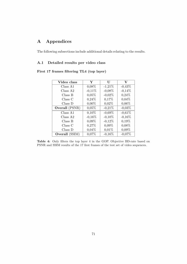
A Appendices

The following subsections include additional details relating to the results.

A.1 Detailed results per video class

First 17 frames filtering TL4 (top layer)

Video class Y U V

Class A1 0,08% -1,21% -0,43%Class A2 -0,11% -0,08% -0,14%Class B 0,05% -0,02% 0,24%Class C 0,24% 0,17% 0,04%Class D 0,00% 0,02% 0,06%

Overall (PSNR) 0,05% -0,21% -0,03%

Class A1 0,10% -0,69% -0,61%Class A2 -0,16% -0,10% -0,16%Class B 0,09% -0,12% 0,19%Class C 0,27% 0,09% 0,08%Class D 0,04% 0,01% 0,09%

Overall (SSIM) 0,07% -0,16% -0,07%

Table 4: Only filters the top layer 4 in the GOP. Objective BD-rate based onPSNR and SSIM results of the 17 first frames of the test set of video sequences.

71

First 17 frames filtering TL3 to TL4

Video class Y U V

Class A1 0,33% -1,06% -1,12%Class A2 -0,19% -0,22% -0,17%Class B 0,15% -0,21% -0,42%Class C 0,36% 0,53% 0,08%Class D 0,10% -0,37% -0,19%

Overall (PSNR) 0,15% -0,26% -0,37%

Class A1 0,53% 0,84% -1,25%Class A2 -0,16% -0,12% -0,16%Class B 0,22% -0,28% -0,44%Class C 0,52% 0,62% -0,32%Class D 0,18% -0,07% 0,15%

Overall (SSIM) 0,26% 0,17% -0,40%

Table 5: Filters temporal layer 3 and 4 in the GOP. Objective BD-rate based onPSNR and SSIM results of the 17 first frames of the test set of video sequences.

First 17 frames filtering TL2 to TL4

Video class Y U V

Class A1 0,29% -2,93% -1,31%Class A2 -0,17% -0,76% -0,13%Class B 0,16% 0,07% -0,28%Class C 0,41% 0,48% 0,41%Class D 0,15% -0,17% 0,08%

Overall (PSNR) 0,17% -0,63% -0,25%

Class A1 0,37% -0,53% -1,85%Class A2 0,06% -0,48% 0,00%Class B 0,18% -0,17% -0,15%Class C 0,84% 0,99% 0,58%Class D 0,33% -0,09% 0,02%

Overall (SSIM) 0,35% -0,06% -0,27%

Table 6: Filters temporal layer 2, 3 and 4 in the GOP. Objective BD-rate basedon PSNR and SSIM results of the 17 first frames of the test set of video sequences.

72

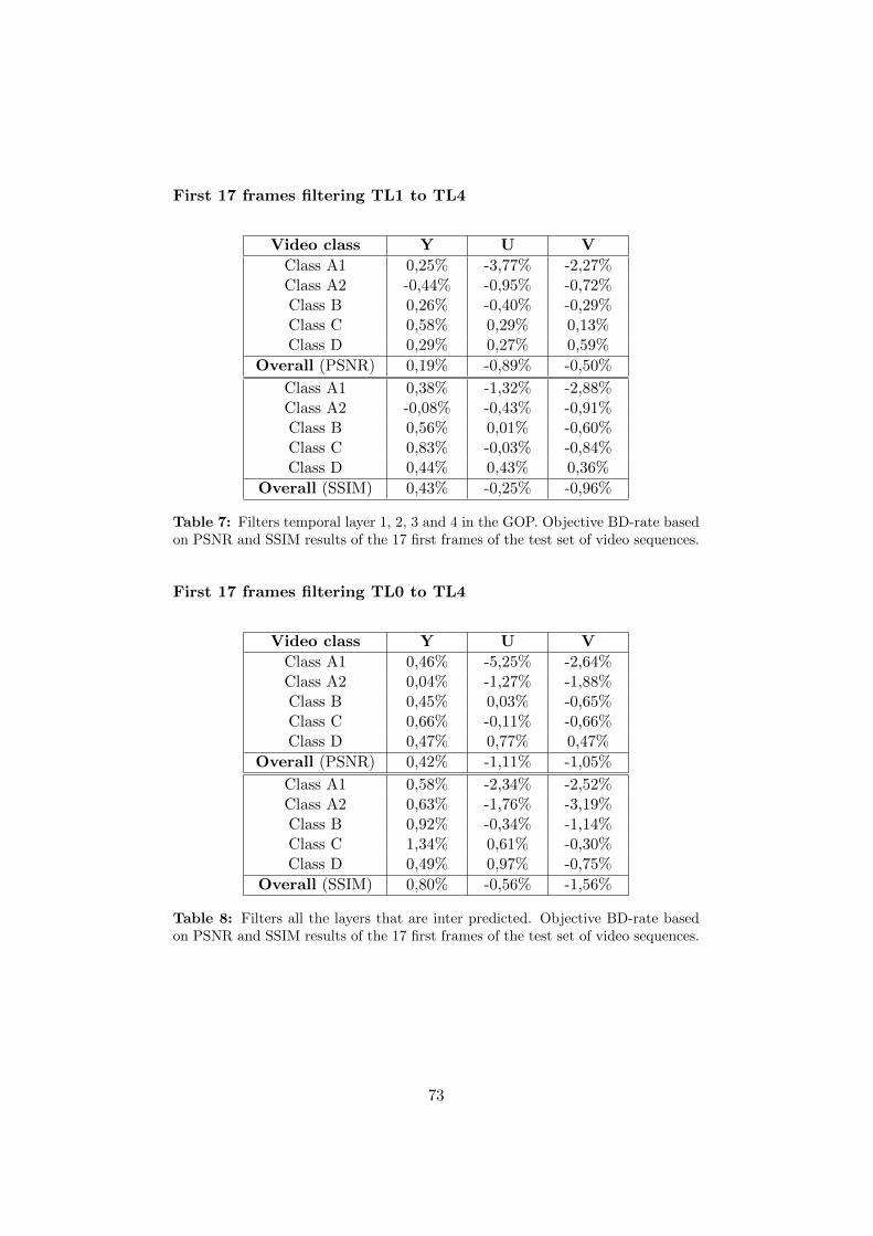
First 17 frames filtering TL1 to TL4

Video class Y U V

Class A1 0,25% -3,77% -2,27%Class A2 -0,44% -0,95% -0,72%Class B 0,26% -0,40% -0,29%Class C 0,58% 0,29% 0,13%Class D 0,29% 0,27% 0,59%

Overall (PSNR) 0,19% -0,89% -0,50%

Class A1 0,38% -1,32% -2,88%Class A2 -0,08% -0,43% -0,91%Class B 0,56% 0,01% -0,60%Class C 0,83% -0,03% -0,84%Class D 0,44% 0,43% 0,36%

Overall (SSIM) 0,43% -0,25% -0,96%

Table 7: Filters temporal layer 1, 2, 3 and 4 in the GOP. Objective BD-rate basedon PSNR and SSIM results of the 17 first frames of the test set of video sequences.

First 17 frames filtering TL0 to TL4

Video class Y U V

Class A1 0,46% -5,25% -2,64%Class A2 0,04% -1,27% -1,88%Class B 0,45% 0,03% -0,65%Class C 0,66% -0,11% -0,66%Class D 0,47% 0,77% 0,47%

Overall (PSNR) 0,42% -1,11% -1,05%

Class A1 0,58% -2,34% -2,52%Class A2 0,63% -1,76% -3,19%Class B 0,92% -0,34% -1,14%Class C 1,34% 0,61% -0,30%Class D 0,49% 0,97% -0,75%

Overall (SSIM) 0,80% -0,56% -1,56%

Table 8: Filters all the layers that are inter predicted. Objective BD-rate basedon PSNR and SSIM results of the 17 first frames of the test set of video sequences.

73

First 50 frames filtering TL4 (top layer)

Video class Y U V

Class A1 0,18% -2,15% -0,90%Class A2 0,04% 0,08% 0,09%Class B 0,08% 0,35% 0,17%Class C 0,38% 0,07% 0,30%Class D 0,17% 0,13% 0,09%

Overall (PSNR) 0,17% -0,27% -0,04%

Class A1 0,13% -1,65% -0,85%Class A2 -0,05% 0,11% 0,04%Class B 0,12% 0,06% 0,19%Class C 0,38% -0,31% 0,05%Class D 0,28% 0,08% 0,30%

Overall (SSIM) 0,17% -0,32% -0,04%

Table 9: Only filters the top layer 4 in the GOP. Objective BD-rate based onPSNR and SSIM results of the 50 first frames of the test set of video sequences.

First 50 frames filtering TL3 to TL4

Video class Y U V

Class A1 0,32% -1,38% -1,42%Class A2 -0,07% -0,03% 0,10%Class B 0,18% -0,15% -0,20%Class C 0,47% 0,42% 0,09%Class D 0,30% 0,08% -0,07%

Overall (PSNR) 0,24% -0,21% -0,29%

Class A1 0,48% -0,37% -1,40%Class A2 -0,09% 0,03% 0,04%Class B 0,29% -0,15% -0,04%Class C 0,68% 0,27% -0,51%Class D 0,52% 0,15% 0,17%

Overall (SSIM) 0,37% -0,02% -0,33%

Table 10: Filters temporal layer 3 and 4 in the GOP. Objective BD-rate based onPSNR and SSIM results of the 50 first frames of the test set of video sequences.

74

First 50 frames filtering TL2 to TL4

Video class Y U V

Class A1 0,32% -2,26% -1,65%Class A2 0,03% -0,14% 0,43%Class B 0,18% 0,14% -0,13%Class C 0,55% 0,41% 0,18%Class D 0,45% 0,11% 0,16%

Overall (PSNR) 0,30% -0,32% -0,20%

Class A1 0,47% -1,24% -1,63%Class A2 0,07% -0,11% 0,24%Class B 0,36% 0,23% -0,12%Class C 0,88% 0,66% -0,05%Class D 0,77% 0,16% 0,46%

Overall (SSIM) 0,50% -0,05% -0,22%

Table 11: Filters temporal layer 2, 3 and 4 in the GOP. Objective BD-rate basedon PSNR and SSIM results of the 50 first frames of the test set of video sequences.

First 50 frames filtering TL1 to TL4

Video class Y U V

Class A1 0,33% -2,75% -2,47%Class A2 -0,03% -0,34% -0,33%Class B 0,28% -0,31% 0,14%Class C 0,61% 0,62% 0,47%Class D 0,64% 0,57% 0,94%

Overall (PSNR) 0,36% -0,44% -0,23%

Class A1 0,54% -1,65% -2,54%Class A2 0,10% -0,10% -0,42%Class B 0,53% 0,01% -0,23%Class C 1,02% 0,21% -0,23%Class D 1,03% 0,86% 0,75%

Overall (SSIM) 0,64% -0,13% -0,52%

Table 12: Filters temporal layer 1, 2, 3 and 4 in the GOP. Objective BD-ratebased on PSNR and SSIM results of the 17 first frames of the test set of videosequences.

75

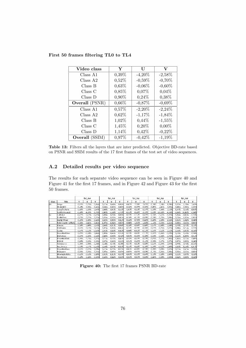
First 50 frames filtering TL0 to TL4

Video class Y U V

Class A1 0,39% -4,20% -2,58%Class A2 0,52% -0,59% -0,70%Class B 0,63% -0,06% -0,60%Class C 0,85% 0,07% 0,04%Class D 0,90% 0,24% 0,38%

Overall (PSNR) 0,66% -0,87% -0,69%

Class A1 0,57% -2,20% -2,24%Class A2 0,62% -1,17% -1,84%Class B 1,02% 0,44% -1,55%Class C 1,45% 0,20% 0,00%Class D 1,14% 0,42% -0,22%

Overall (SSIM) 0,97% -0,42% -1,19%

Table 13: Filters all the layers that are inter predicted. Objective BD-rate basedon PSNR and SSIM results of the 17 first frames of the test set of video sequences.

A.2 Detailed results per video sequence

The results for each separate video sequence can be seen in Figure 40 andFigure 41 for the first 17 frames, and in Figure 42 and Figure 43 for the first50 frames.

Figure 40: The first 17 frames PSNR BD-rate

76

Figure 41: The first 17 frames SSIM BD-rate

Figure 42: The first 50 frames PSNR BD-rate

Figure 43: The first 50 frames SSIM BD-rate

77