Inter-Active Learning of Ad-Hoc Classifiers for Video Visual Analytics

Benjamin Hoferlin∗a, Rudolf Netzel† b, Markus Hoferlinb, Daniel Weiskopfb, Gunther Heidemanna

aInstitute of Cognitive Science, University of OsnabruckbVisualization Research Center (VISUS), University of Stuttgart

ABSTRACT

Learning of classifiers to be used as filters within the analytical rea-soning process leads to new and aggravates existing challenges.Such classifiers are typically trained ad-hoc, with tight time con-straints that affect the amount and the quality of annotation dataand, thus, also the users’ trust in the classifier trained. We ap-proach the challenges of ad-hoc training by inter-active learning,which extends active learning by integrating human experts’ back-ground knowledge to greater extent. In contrast to active learning,not only does inter-active learning include the users’ expertise byposing queries of data instances for labeling, but it also supportsthe users in comprehending the classifier model by visualization.Besides the annotation of manually or automatically selected datainstances, users are empowered to directly adjust complex classifiermodels. Therefore, our model visualization facilitates the detec-tion and correction of inconsistencies between the classifier modeltrained by examples and the user’s mental model of the class defini-tion. Visual feedback of the training process helps the users assessthe performance of the classifier and, thus, build up trust in the filtercreated. We demonstrate the capabilities of inter-active learning inthe domain of video visual analytics and compare its performancewith the results of random sampling and uncertainty sampling oftraining sets.

Index Terms: H.3.3 [Information Systems]: Information Storageand Retrieval—Information Search and Retrieval; I.2.6 [ComputingMethodologies]: Artificial Intelligence—Learning

1 INTRODUCTION

Reduction of data to its relevant parts is a central and recurrent stepof the visual analytics process, as outlined in the visual analyticsmantra [17]: “Analyse First – Show the Important – Zoom, Filterand Analyse Further – Details on Demand”. Such reduction is crit-ical for data scalability and is performed by automatic methods oruser-defined filters. While automatic methods reduce the amount ofdata by exploiting some structure or by calculating predefined fea-tures and statistics, filters serve as their equivalents in human visualinformation seeking. Filters are involved in both exploratory inter-action to reduce the amount of data displayed and to focus on thedetails (e.g., by dynamic queries [29]) and in confirmatory interac-tion to confirm or refute hypotheses about the data (e.g., in videovisual analytics [15]). Typically, users define filters by providingmodel parameters or examples of data instances they want to beincluded in, or excluded from, their query.

We focus on the question how filters can be efficiently defined.This question arises especially when analyzing complex and high-dimensional data spaces, where appropriate model parameters areunknown and filter definition by a single example is too weak. Insuch cases—we will use the examples of data and tasks from video

∗e-mail:benjamin.hoeferlin@uni-osnabrueck.de†e-mail:rudolf.netzel@visus.uni-stuttgart.de

visual analytics throughout the paper—query by multiple examplescan be useful, which is identical to the training of a complex clas-sifier. In this way, users can specify what they seek by integrat-ing machine learning techniques into information visualization, ascommonly recommended (e.g., by Shneiderman [30] or Chen [6]).However, in contrast to pre-trained classifiers as they are widelyused in video analytics (e.g., person or car detectors, included inmany video management systems), classifiers used to define filterswithin the visual analytics process have to be trained ad-hoc.

Such ad-hoc trained classifiers for filtering are required withinthe sense-making loop of analysts [35], when they build a case orsearch for support or evidence for a hypothesis within the data. Letus consider the example of video surveillance operators who as-sume, after some initial analysis of video sequences, that a cyclistmight have been involved in the case of a traffic incident they dealwith. Hence, they want to extract cyclists from video data to reducethe amount of video and to focus on promising parts for hypoth-esis verification. This example illustrates the need for training ofnew and arbitrary classifiers that can also be highly complex andspecialized (e.g., hand-waving bicyclists with red helmets may beimportant in our example scenario). Since pre-trained instances ofsuch classifiers are generally not available, the analysts have to de-fine the filter by themselves. However, feature selection and modelparameter definition for objects such as a bicyclist are too complexto be manually defined, even for domain experts with support byinteractive visualization [43]. Hence, filter definition via query byexamples promises to be the only viable solution.

In contrast to traditional supervised training of a classifier, ad-hoc training involves new challenges:Annotation Costs: Data annotation is a very costly task becausea large amount of annotated data is required for proper training ofa classifier. Furthermore, the data has often to be annotated by do-main experts in a time-consuming process. These facts question thebenefit of ad-hoc training of filters within the analytical reasoningprocess. In addition, the issue of decreasing analysis performancearises if disruption that comes with high time consumption for train-ing influences the analysis process. Finally, to find appropriate ex-amples that can be labeled tends to be a difficult task that becomesworse with the rareness of the data instances queried (imagine thesearch for hand-waiving cyclists with red helmets).Annotation Quality: A typical phenomenon of positive exampleselection in ad-hoc training scenarios is that the provided data in-stances are not sampled as independent and identically distributedrandom variables from the query distribution, as required by thelearner. In fact, users tend to provide samples drawn from a rathersmall region in data space. This effect obviously increases with therareness of suitable examples in the data: if a hand-waiving cyclistwas found, he will be annotated in all frames of the video. Althoughthis approach provides multiple training examples, the training setitself is very specialized and may not generalize to all instances ofthe intended query (e.g., all hand-waiving cyclists). Furthermore,the quality of annotated examples is affected by the often vagueidea of the query the users have in mind when defining the filter.The question of the exact range of the data instances of interestmay arise (e.g., is a person on a trike also of interest?). This issue isfurther intensified in data domains where no clear data instances are

23

IEEE Conference on Visual Analytics Science and Technology 2012October 14 - 19, Seattle, WA, USA 978-1-4673-4753-2/12/$31.00 ©2012 IEEE

Data

Labels

LearnerModel

DataLearnerModel

U

BootstrapExamples

Understand

Manipulate

Select

Select

Labels

L

Annotation Retrain

(a) (b)

Figure 1: (a) Data flow of passive supervised machine learning. A training set (data + large amount of labels) is provided to the learner, either asa monolithic set (batch learning) or in many smaller pieces (online learning). (b) In active learning, a bootstrapped learner iteratively refines itselfby posing queries from a pool of unlabeled data U to a (human) oracle that provides labels for the data L. Inter-active learning is an extension(red arrows) of active learning that further allows the human experts to directly integrate their background knowledge into the model.

predefined. For example, we encounter the question how a data in-stance should be defined in object or event detection for video anal-ysis: is the object silhouette the right way to crop the example fromthe video frame or can we use a bounding rectangle to define theimage region, and if so, does the precision of the rectangle affectthe filter performance? Such questions will not arise in domainswhere precisely defined documents are available, as it is the casein text document retrieval or content-based image retrieval. Theseissues especially arise in the ad-hoc training context. We will referto them by the term annotation noise (see Fig. 2).Classifier Quality Assessment: A general question in machinelearning is to detect the appropriate moment when to stop train-ing of a classifier. The classifier should well adapt to the trainingdata, but be general enough to correctly classify unseen data in-stances, too. This overfitting issue is traditionally tackled by crossvalidation. However, this approach requires either much more an-notated examples for a validation set or much more time, since mul-tiple classifiers have to be trained on different subsets of the trainingset. Furthermore, the generalization assessment of the classifier bycross validation is limited by the sampling bias induced by ad-hocannotation (cf. annotation quality). Thus, cross validation is hardlyfeasible and often undesired in the ad-hoc training context. A ques-tion related to the stopping criteria in training is the question ofstopping criteria in annotation of examples. This issue is of practi-cal relevance because annotation involves costs. However, often noappropriate measure of training progress is available that facilitatesthe definition of such stopping criteria [36]. Finally, quality assess-ment of the classifier becomes important to ad-hoc training becausethe users have to develop trust in their defined and applied filters.Hence, it is important to them to judge their classifier’s performancewhen it is faced with unseen data or noisy data.

Training of a classifier under the constraint of high annotationcost is tackled by the field of active learning. In contrast to tradi-tional supervised machine learning (see Fig. 1 (a)), an active learneris allowed to choose the data from which it wants to learn. Thisway, typically greater accuracy can be achieved with fewer train-ing labels. As depicted in Fig. 1 (b), active learning is an iterativeprocess of refinement in which the learner may pose queries of un-labeled data to an oracle (e.g., a human) that provides the labels forthis data. The active learner typically queries labels for the datainstances with the highest informativeness or those that promiseto reduce uncertainty most. Settles [27] and Olsson [21] providean introduction and comprehensive overview of the field of activelearning. For a survey of the application of active learning for mul-timedia annotation, we refer to Wang and Hua [41].

Theoretical analysis has shown that an active learner (however,a computationally complex query-by-committee approach) can re-

duce the complexity of required labels in exponential order [10].Empirical analysis reveals that in the majority of applications, ac-tive learning is able to reduce the amount of labels [27], too. A sur-vey of the usage of active learning for text annotation exhibits thatthe expectations of most practitioners on the performance of activelearning are either fully (36.3%) or partially (54.4%) met [36]. Thereduction of examples to label in practical situations, however, maylie far behind exponential decrease and, dependent on the dataset,sometimes does not show any improvement at all [24]. Further,some authors report negative results [11, 13] or show that the per-formance depends on the expertise of the annotator [2].

Due to these results and the further challenges that we face inthe context of ad-hoc training, we question whether active learningalone is suitable for ad-hoc training and capable of meeting the tighttime constraints existing in this application. Furthermore, we ques-tion the idea of the human experts as mere annotators, but believethat their expertise should be utilized in a more direct way.

In this paper, we introduce a novel method called inter-activelearning, an extension to conventional active learning that directlyinvolves human experts in the ad-hoc training process using the vi-sual analytics methodology. The additional interaction introducedby inter-active learning is depicted by red arrows in Fig. 1 (b): thegoal of this process is to efficiently create filters leveraging the com-plementary strengths of human and machine, as outlined by Bertiniand Lalanne [4] in the context of the knowledge discovery process.

In detail, inter-active learning efficiently approaches the goal ofa well-trained classifier by iterating over the three basic steps: i) as-sessment of the performance of the classifier, ii) annotation of datainstances and/or manipulation of the classifier model, and iii) re-training of the classifier. In Section 3, we will break down thesebasic steps into different tasks the users perform in each cycle toincorporate new background knowledge into the trained model.

This paper contributes to the current state of research by present-ing a way how the problem of ad-hoc training of classifiers for in-teractive filter definition can be tackled by visual analytics. Besidesintroducing a general methodology, which can be considered as anextension of active learning methods toward increasing leverage ofthe users’ expertise, we apply inter-active learning to the domainof video analysis for validation. We present an integrated visualanalytics system that covers the three steps of inter-active learningand provides an adaption to online learning of the cascade classi-fier model we use, as well as visualization and interaction modelsthat can cope with the complexity, high dimensionality, and hugeamount of data of the video domain. A usage scenario illustratesthe different tasks the users carry out within the three steps and fur-ther provides validation of our method by comparison to classifiertraining with random sampling and uncertainty sampling.

24

2 RELATED WORK

Our approach is related to techniques from visual analytics, knowl-edge discovery, data mining, information visualization, and ma-chine learning. Closely related is previous work by Seifert andGranitzer [25], Seifert et al. [26], May and Kohlhammer [18], andHeimerl et al. [14]. All four methods aim at tight integration ofthe user into the labeling process. The first work [25] presents auser-based and visually supported active learning method that wassuccessfully validated on different multi-class datasets of variousdata domains. Seifert et al. [26] focus on visual classifier perfor-mance assessment, while the learner can be adapted by labelingdata instances in an information landscape visualization. Valida-tion is provided by means of a multi-class, multi-label text classifi-cation scenario. May and Kohlhammer [18] also allow the user torefine a classifier model by selection of training examples. They fo-cus on performance feedback of the classifier model using a visual-ization that facilitates pre-attentive pattern identification. Recently,Heimerl et al. [14] have introduced a system to interactively traina support vector machine model for text document retrieval basedon visual analytics and active learning. Further, they provided athorough evaluation of their approach. However, all four methodsdo not go beyond interactive definition of the training set and userselection of the data instances to label. More direct integration ofhuman experts’ background knowledge is not considered.

There are several approaches of interactive definition of clas-sifiers (e.g., [1, 8, 32, 34, 43]), that do not consider support of(semi-) automatic methods for classifier refinement, such as activelearning. Although these methods were successfully applied to trainor combine classifiers, purely user-based definition of classifiersseems only to be viable for problems with low complexity [43]; oth-erwise, they annoy the users by recurring tasks [32]. Furthermore,interactive definition often constrains the complexity of the classi-fier model; hence, decision trees typically appear in these works.

Another approach incorporating the users’ background knowl-edge into the training process is followed by the active learningcommunity. In the domain of text classification, where features of-ten coincide with words, promising methods were developed thatallow the learner to pose queries to the oracle to label features,instead of just data instances [28, 31]. This means that the ora-cle can tell the learner if a particular feature describes a particularclass well. However, feature labeling can only be applied in ar-eas where features are tangible to human users (e.g., word featuresin text classification). Thus, such methods are not applicable incomplex and abstract problem environments in which features donot exhibit any concrete symbolic meaning to humans. Besides themethods that incorporate human decisions in machine learning, vi-sualizations of classifier models for performance assessment andmodel understanding, such as [3, 5, 19], are naturally related to ourapproach. In contrast to the existing approaches, we advance thefields of active learning and visual classifier definition by combin-ing them to a visual analytics process called inter-active learning.

3 INTER-ACTIVE LEARNING

In this section, we outline the theoretical considerations of inter-active learning and specify its requirements for learning models,visualization, and interaction.

Inter-active learning re-formulates the problem of supervisedmachine learning as a visual analytics problem. Supervised ma-chine learning for classification, as depicted in Fig. 1 (a), seeks tofind model parameters m that minimize the class confusion error E(according to the distance function ferror) of the classifier functionhm : S→ T , which maps the data distribution S to a set of targetclasses T = {0,1, · · · ,n}:

E = ∑i∈I

ferror(hm(si), li)

Here, a training vector of data/label pairs (si, li) is provided, wheredata samples si are drawn as independent and identically distributedrandom variables from S and data labels li =L (si) are given by thelabeling function L ; I denotes the set of sample indicies. We donot consider any further regularization terms, such as smoothnessof the function.

In contrast to passive supervised learning, active learning addi-tionally minimizes the costs C = ∑i∈I C (L (si)) that arise by ac-quiring a finite set of labels li. Active learners are allowed to posequery of data instances to be labeled to the users. The decisionwhich data has to be labeled for the next training cycle dependson the current model m, the available data instances si ∈ U, andthe labeling costs. Active learners typically assume a uniform costfunction C (i.e., C = |I|) and thus query labels for the most infor-mative data instances from the users. This process is illustrated fora pool-based active learner in Fig. 1 (b) (ignoring the red arrows).

Inter-active learning, as an extension to active learning, pursuesthe same objective: a well-trained classifier trained with minimallabeling costs. In contrast to active learning, inter-active learningassumes that the users—based on their expertise of the domain andtheir knowledge about m—are able to select a more effective setof data instances to be labeled. Further, the training process canbenefit from direct modifications of the learner model m. In high-dimensional data domains with complex dependencies, however,direct definition of model parameters can be difficult [43]. Hence,we focus on permitting the users to detect and solve contradictionsbetween their domain knowledge and the actually trained model m.

data noise

annotation noise

model q

ualit

y

(re-)train

active query

man

ual q

uery

& an

nota

tion m

odification

Figure 2: Major components and information flow involved in theinter-active learning process. Solid lines depict information conveyedto the users by visualization, dashed lines represent user interaction,and dotted lines illustrate the flow of information triggered by auto-matic methods. Furthermore, the contribution of noise-affected dataand labels to the model’s uncertainty is depicted.

Due to the tight connection between learner and user, visualiza-tion and human-computer interaction are, besides automatic meth-ods, the central aspects of inter-active learning. Figure 2 illustratesthis connection between the three major elements: learner model,user, and data. Furthermore, Fig. 2 depicts the flow of informa-tion between the three elements that can be assigned to one of thethree category of methods: visualization, interaction, or automaticmethod. The iterative interaction of these three components resultsin a visual analytics process that aims to refine the classifier modeland its comprehension by the users.

Each cycle of this iterative process consists of three steps men-tioned before: i) assessment of the model performance, ii) refine-ment of the classifier model, and iii) retraining of the classifier. Thefirst two steps, which include user interaction, can further be di-vided into tasks the users may consider to process each cycle. Forthe first step, these tasks include assessing the success of the last

25

training cycle (training feedback) and determining if a stopping cri-terion was reached (e.g., the model has already reached an appro-priate level of quality or training does not improve the model any-more). Furthermore, by assessing the model’s performance, userscan build trust in their trained model and learn to know its strengthsand weaknesses. Hence, they can incorporate the performance anduncertainty of “their” filters into their decisions within the analyt-ical reasoning process. Finally, quality assessment also guides theusers in refining the model. Users may detect overfitting of themodel, low robustness to noise, or lack of generalization. Theseissues are tackled in the second step of a cycle.

After the classifier model was analyzed in the first step, two typesof refinement are available to the users in the second step: data an-notation and model manipulation. While both data annotation andmodel manipulation can be used to broaden the classifier model toaccept a wider variety of data instances or to narrow the accep-tance range, we recommend using model manipulation mainly forgeneralization purposes; in contrast, data annotation is suitable forboth tasks. This recommendation accounts for the complex depen-dencies of high-dimensional data distributions. In such cases, it isoften easier to tell the system what is wrong (e.g., overfitting of themodel) than to define what is right. For data labeling, the users canchoose which data regions they intend to annotate for model refine-ment. In this way, the users can efficiently integrate novel domainknowledge into the system. Labeling of data in regions near the de-cision boundaries helps increase the classifiers confidence, whereaslabeling of data in regions far away from the decision boundaryhelps explore new regions of the data space and might reduce ex-tensive class confusion. However, users can also rely on the classi-fier model to provide the most beneficial data instances for labelingutilizing active learning.

In the next sections, we introduce the main components of avisual analytics system for inter-active learning and explain theirapplication for the tasks mentioned above. These components in-clude, besides different (coordinated) views on the data and model,also the definition and implementation of an appropriate classifiermodel. Furthermore, we will address issues of scalability and inputnoise that affects the trained model.

4 CLASSIFIER REQUIREMENTS

In this section, we describe the requirements for a learner for ad-hoc training in general and the classifier model we use for videovisual analytics in particular.

Filters generated by ad-hoc training have to be of low time com-plexity because such filters are often used to facilitate scalabilitywith increasing data size. In this paper, we use a cascade of clas-sifiers (Fig. 3 (b)) to predict class assignments of sliding windowsin each video frame. In combination with a set of basic, yet fast tocompute, rectangle features, this method has become popular withthe work of Viola and Jones [39] in the context of face detection.Rectangle features (Fig. 3 (a)) operate on gray-value images and arecomputed by subtracting the sum of pixel values of the black partfrom the sum of pixels of the white part.

Similar to Viola and Jones, we also use a committee of thresh-olded rectangle features as weak classifiers within each node ofthe cascade. The features for each node are typically selected andweighted by some boosting algorithm, such as AdaBoost [9]. Thehigh efficiency of the cascade during evaluation of sliding win-dows (various rectangular cropped parts of the video frame) re-sults from the low complexity of the first nodes. With only fewcomputations, the first node already rejects about half of all slidingwindows; the complexity and number of features typically increasewith each node. Sliding windows that pass all nodes in the cascadeare considered detections (Fig 3 (b)), such as the sliding window inFig 3 (a), which contains a person onto whom the rectangle featureselected is superimposed and aligned by boosting. This often ap-

c1 c2 c3

No Detection

DetectionSearchWindow

No Detection No Detection

(a) (b)

Figure 3: (a) Six prototypical rectangle features and a cropped part ofa sliding window containing a detected person onto whom one of therectangle features superimposed. (b) Each node of the cascade ofclassifiers makes a binary decision on the sliding window: whether itis dropped or processed by the next classifier node. Sliding windowsthat process the whole cascade are considered to be detections.

plied approach only distinguishes between sliding windows that are“detected” by the cascade or not, hence it defines a binary classifi-cation problem. If not stated otherwise, the parameters we use forour cascade of classifier are derived from the original work of Violaand Jones [39].

As reported by Tomanek and Olsson [36], it is critical for in-teractive refinement of classifiers that retraining can be performedvery fast to keep the idle time of users at an acceptable level. Failsand Olsen [8] even claim that, in order to be effective, the classifiermust be generated from the training examples in under five seconds.These requirements also apply to inter-active learning. Hence, mosttraining algorithms are not suitable for inter-active learning becausethey tend to need several hours of time for learning the model basedon a huge set of labeled data. However, by retraining the classifierwith only the samples the users labeled in the current cycle, wecan meet the efficiency requirements. Methods that can iterativelyupdate the model according to newly provided data/label pairs arecalled online training methods.

In this paper, we use a modified version of online AdaBoost, in-troduced by Oza [23]. Since in online training, the learner is facedwith only one example a time, the basic idea of online boosting is tomaintain statistics for each feature that capture its performance his-tory for all the samples seen so far. This, however, implies thatgreedy selection of features cannot consider the complete set ofexamples when choosing a particular feature, since future exam-ples are not available. Hence, the performance of online AdaBoostapproaches the performance of batch-mode training in the limit.Based on the introduced statistics, an estimated error ei can be cal-culated for each weak classifier. A weak classifier hweak

i is builtfrom a rectangle feature i that is thresholded after evaluation to ob-tain a binary decision (i.e., hweak

i ∈ {−1,1}); hence, we use theterms feature and weak classifier interchangeably.

A subset of all available weak classifiers is selected by the greedyboosting algorithm according to the lowest error to form a strongclassifier hstrong. The binary decision about the class assignment ofeach sliding window s is made in each node of the cascade by itsrespective strong classifier hstrong. Therefore, the weighted sum ofbinary responses of all n boosted weak classifiers that belong to thestrong classifier and threshold t are used:

hstrong(s) = sign(conf(s)− t)

conf(s) =n

∑i=1

aihweaki (s) (1)

ai = log(

1− ei

ei

)AdaBoost lives on rating the importance of each example for train-ing (a correctly classified example is of lower importance than an

26

incorrectly classified one). Online AdaBoost estimates the impor-tance of an example for each feature based on the binary decisionsof the preceding weak classifiers. According to the estimated im-portance, the history maintained by each feature is influenced.

Training of a node means to adjust the thresholds, weights, andhistory of all features. The approach of Oza only uses a fixed num-ber of features. We improve on this by integrating the idea of Grab-ner and Bischof [12]. They use selectors to dynamically choose thecommittee of weak classifiers with the best performance out of anumber of features that are constantly trained. In this way, chang-ing number of features also becomes possible.

Each strong classifier of the cascade is trained with a modifiedversion of this online AdaBoost algorithm. The main improvementswe make to the method of Grabner and Bischof affect the statis-tics maintained for each strong classifier. By introducing two his-tograms (one for the positive and one for the negative examples) ofthe conf measure (see Equation (1)), we enable a cascade construc-tion that is similar to the original algorithm by Viola and Jones. Us-ing the histogram of confidences of positive training examples, thetrue positive rate can be adjusted to match the classification goalsof a node by decreasing the threshold t to an appropriate level. Thefalse positive rate is then accessible by the confidence histogram ofnegative examples, by summing up the bins between one and thecurrently chosen threshold. After the cascade node was trained byan example, either the former or the latter histogram, is updated (de-pending on the label of the data example) by increasing the particu-lar bin by α . Finally, the histogram is normalized to one. The con-stant α controls the decay rate that is necessary because the storedconfidence values become outdated by training. In our examples,we use an experimentally derived value of α = 2/η , with η beingthe number of samples seen so far.

To increase robustness for imbalanced numbers of positive andnegative training examples, we modify the boosting algorithm tooptimize the distance between the receiver operating characteristic(ROC) of the node’s classification history and the point of optimalclassification (i.e., TPR= 1, FPR= 0), involving calculation of truepositive rate (TPR) and false positive rate (FPR) of each weak clas-sifier. New nodes are added to the cascade until the maximum errorrate FPRoverall > FPRoverall = ∏

mk (FPRk) is met. For our experi-

ments, we choose an maximum error rate consistent with Viola andJones [39]: FPRoverall = 10−5. Finally, we enable the users to mod-ify the cascade, by adding new features (user-defined features) toa node or changing the position or shape of features that were se-lected by the algorithm.

5 ACTIVE LEARNING

When users lack the knowledge which data instances are most effi-cient to label, they can use active learning. Pressing a button, theyautomatically obtain a selection of data instances for which the ac-tive learner is most uncertain. The selection is shaped by a pool-based uncertainty sampling approach. For the cascade of classifierswe use, uncertainty u about the true label of a sliding window scorresponds to a sum of confidence (Equation (1)) values of all mnodes involved in making the class decision:

u(s) =1

∑mk=1 confk(s)

(2)

This is equivalent to the definition of confidence by Visentini etal. [40] and Graber and Bischof [12]. The most uncertain data in-stances will be selected to be further analyzed by the users.

6 VISUALIZATION AND INTERACTION

In this section, we introduce the different views and interactiontechnique of our inter-active learning framework. The screenshotof the workspace depicted in Fig. 4 shows the three main areas of

the graphical user interface (GUI). Left, we see the trained classifiermodel (Fig. 4 (b)) and the cascaded scatterplot (Fig. 4 (a)) showingthe evaluation results of the cascade for performance assessment.On the right, three different views on the model and data are avail-able for annotation and model modification, which are used in thesecond step of each training cycle. In-between both GUI areas,the current selection of data instances, cascade nodes, and featuresis shown (Fig. 4 (c)). The selections connect the performance as-sessment step with the refinement step and, in this way, provide anatural arrangement of tasks. For interpretability, a distinct color isassigned to each type of selection. This color is used to highlightthe selection in each of the coordinated views.

6.1 Cascaded ScatterplotTo present the feedback on the quality of the current classifier, weintroduce a novel visualization of the class distribution of data in-stances (sliding windows of the video) in each stage of the classi-fier. This visualization, which we call cascaded scatterplot, inte-grates multiple dependent scatterplots that are horizontally alignedto match with the cascade information (Figs. 4 (a) and (b)).

In the cascaded scatterplot, the abscissa is divided into m parts,with m being the number of nodes in the cascade. In contrast toconventional scatterplots, cascaded scatterplots represent each datapoint up to m times. Coordinates of a data point in the cascadedscatterplot depend on the classification quality of the sliding win-dow s by the respective strong classifier (cascade node). The x-value of each instance of a data point is made up of an integervalue that determines its assignment to a cascade node as well as ofa fractional part that represents the confidence of each classifier’sdecision on the data point. Hence, data points of two classifierscannot overlap in their x-value. For each data point and classi-fier, we plot the normalized confidences (distance to the decisionboundary on the x-axis) ck(s) ∈ [−1;1] against the feature robust-ness rk(s) ∈ [0;1] (y-axis) for each node Nk.

The robustness rk(s) of a feature decision is influenced by twocomponents: the robustness of the feature weights rweight of eachnode with nk features, and the distance between the feature responseof the signal and the threshold of the feature (its decision boundary)rmargin. Together, the feature robustness rk(s) = rweight

k rmargink (s) in-

dicates the reciprocal of the influence of signal noise on the decisionof the strong classifier Nk. The robustness of the feature weightsrweightk utilizes the normalized entropy of the feature weights ai to

penalize the skew of weight distribution to a small amount of hugeweights because in this case, the decision of a node may be changedonly due to the flipping a couple of its features’ decisions:

rweightk =− ∑

i∈Nk

ai log(ai)

log(nk)

Data instances with a small distance between their feature responseand the feature’s threshold are likely to flip the weak classifier’sdecision in the presence of noise. Therefore, rmargin

k includes theaverage distance (normalized to the maximum margin of the fea-tures) between the features’ decision boundaries ti and the signal’sresponse to each feature fi(s):

rmargink (s) =

1nk

∑i∈Nk

|ti− fi(s)|maxmargini

The feature robustness is shown along the y-axis of the scatterplotand helps the users judge the classifiers sensitivity to data noise thatinfluences the general quality of the model. On the x-axis, the un-certainty of the class assignment is shown by the distance of thedata points to the decision boundary of each strong classifier in thecascade. The confidence measure ck(s) is normalized to the range

27

Figure 4: Typical workspace of our visual analytics system for inter-active learning after learning with a couple of training examples: (a) cascadedscatterplot, (b) cascade information, (c) selection interface, (d) video context view, (e) visualization of classifier model, (f) annotation view. Detailsof the components can be found in Section 6.

of [−1,1], where ck(s) =−1 and ck(s) = 1 represent confident de-cisions, either negative or positive according the class membershipof the data instance:

ck(s) =confk(s)

∑i∈Nk

∣∣aihweaki (s)

∣∣Besides both boundaries of maximum confidence, we illustrate thedecision boundary (dashed lines in Fig. 4 (a)) at ck(s) = 0 for ori-entation, too. By selecting one or more data points in the cascadedscatterplot representation of a node, the data points will be high-lighted in all other nodes in which they appear. In this way, theusers can easily assess the class assignment and the quality of thedecisions of the selected data throughout the whole cascade. Theassignment of each data instance to either the positive class (e.g.,person) or the negative class (i.e., background region) is indicatedby the respective color (green or red) of the data point in the cas-caded scatterplot for each node. For convenience, the users canchoose to display only positive or negative classifications, or bothcombined in one plot.

In combination with other views, the cascaded scatterplot ismainly used to assess the performance of the classifier and to pro-vide feedback on the training progress. In this way, users gain trustin the trained classifier and may decide to stop the refinement pro-cess, either because no further progress in training is experiencedor the quality of the classifier reached a sufficient level. Recogni-tion of the right point to stop training is of practical relevance, asthe survey by Tomanek and Olsson [36] points out: most of theparticipants had a stopping criteria that would fit the context of ad-hoc training. Furthermore, the cascaded scatterplot is used to selectdata instances for labeling and thus, to avoid overfitting of the clas-sifier, reduce uncertainty of the classification decision, or improvegeneralization by exploring new data regions.

To handle the tremendous amount of data we face in the contextof video analysis, the amount of data displayed can be adjusted bythe user. In this way, we maintain the responsiveness of the interac-tive visualization and reduce overdrawing in the cascaded scatter-plot. The users can define the frame interval and a number of frames

to be evaluated. These will be randomly chosen from the interval.Further, we constrain the number of evaluated data instances, byconsidering only sliding windows that have an aspect ratio similarto the average aspect ratio of the positive training examples.

The displacements dx and dy (measured in pixels (px)) and scal-ing factor s f of the sliding windows are further restricted. Applyingour default values (dx = 5 px, dy = 5 px, and s f = 1.5) results in al-most two million data instances to be evaluated for 50 frames of avideo with 720× 576 px resolution. This shows that evaluating anentire video would exceed the capabilities of human and machinevery quickly. Hence, we provide further constraints to keep theamount of data at a manageable level. Besides random sampling ofa smaller amount of data instances from the video, we use two ad-ditional methods to reduce the amount of data displayed. The firstmethod focuses on relevant regions of the data distribution by inter-active definition of robustness and uncertainty intervals in the cas-caded scatterplot. The second method automatically selects a fixednumber of the most uncertain detections by using active learning.

6.2 Annotation

After data instances have been selected, either by the users or au-tomatically by the active learning subsystem, the data points arevisualized in the annotation view (Fig. 4 (f)). This helps the user tocomprehend the quality of the classifier and discover areas of datainstances that have the wrong class assignment (class confusion).

To facilitate overview and efficient annotation of the data in-stances, we project the data points onto a two-dimensional mapaccording to their similarity. For this purpose, we use the dimen-sion reduction algorithm developed by Van der Maaten and Hin-ton [38], called t-Distributed Stochastic Neighbor Embedding (t-SNE). Van der Maaten and Hinton showed that this method pro-vides good visualizations of high-dimensional data lying on relatedlow-dimensional manifolds, such as images of multiple objects cap-tured from different viewpoints.

We visualize the two-dimensional map provided by t-SNE bydisplaying thumbnails of the sliding windows. Class assignment ofthe classifier as well as data selection is shown by the border color

28

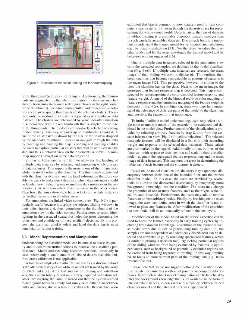
Figure 5: Selection of the initial training set for bootstrapping.

of the thumbnail (red, green, or orange). Additionally, the thumb-nails are augmented by the label information if a data instance hasalready been annotated (small red or green boxes in the right cornerof the thumbnails). To reduce visual clutter and to increase annota-tion speed, overlapping thumbnails are depicted as clusters. There-fore, only the medoid of a cluster is depicted as representative datainstance. The clusters are determined by kernel density estimationin screen-space with a fixed bandwidth that is adapted to the sizeof the thumbnails. The medoids are iteratively selected accordingto their density. This way, any overlap of thumbnails is avoided. Acue of the cluster size is shown by the size of the shadow droppedby the medoid’s thumbnail. Users can navigate through the databy zooming and panning the map. Zooming and panning enablesthe users to explore particular clusters that will be unfolded step bystep and thus a detailed view on their elements is shown. A min-imap supports navigation in the data projection.

Similar to Mohrmann et al. [20], we allow for fast labeling ofmultiple data instances by selecting and annotating whole clustersof data instances. This supports the users in one of their main taskswhile iteratively refining the classifier. The thumbnails augmentedwith the classifier decision and the label information therefore en-able the users to make quick decisions which data instances shouldbe labeled next. Selecting one or multiple data instances in the an-notation view will also select these instances in the other views.Therefore, the annotation view helps select similar data instancesfor further inspection in the other views.

For annotation, the linked video context view (Fig. 4(d)) is par-ticularly useful because it displays the selected sliding windows intheir video frames and, thus, complements the thumbnails of theannotation view by the video context. Furthermore, selection high-lighting in the cascaded scatterplot helps the users determine therobustness and confidence of the classifier’s decision. By this pro-cess, the users can quickly select and label the data that is mostbeneficial for further training.

6.3 Model Representation and Manipulation

Understanding the classifier model can be crucial to assess its qual-ity and to determine further actions to increase the classifier’s per-formance. Model understanding becomes beneficial, especially incases where only a small amount of labeled data is available and,thus, cross validation is not applicable.

A famous example of classifier failure due to a restrictive datasetis the often-cited story of an artificial neural net trained by the armyto detect tanks [7]. After first success on training and validationsets, the system totally failed on a newly captured validation set.After investigating the issue, it turned out that the system learnedto distinguish between cloudy and sunny skies rather than betweentanks and bushes, due to a bias in the data sets. Recent discussion

exhibited that bias is common to most datasets used to train com-puter vision systems [37], even though the datasets strive for repre-senting the whole visual world. Unfortunately, the bias of datasetsin ad-hoc training is presumably disproportionately stronger thanin such carefully assembled datasets. Due to such bias, it is impor-tant to understand the trained model for verification and validation,e.g., by using visualization [33]. We therefore visualize the clas-sifier model and let the users investigate the trained model and itsbehavior, as often suggested [16].

One or multiple data instances, selected in the annotation viewor in the cascaded scatterplot, are depicted in the model visualiza-tion (Fig. 4 (e)). If multiple data instances are selected, the meanimage of their sliding windows is displayed. This outlines theircommonalities that become recognizable as patterns of patterns inthe mean image [42]. This perspective, however, is similar to theview the classifier has on the data. Next to the mean image, thecorresponding feature response map is depicted. This map is con-structed by superimposing the color-encoded feature response andfeature weight. A legend of the bimodal red-blue color mapping offeature response and the luminance mapping of the feature weight isdepicted in Fig. 4 (e). In combination, these two maps help under-stand the relevance of different parts of the model to the classifiersand, possibly, the reason for that importance.

To further facilitate model understanding, users may select a sin-gle node or multiple nodes of the cascade to be evaluated and de-picted in the model view. Further control of the visualization is pro-vided by selecting arbitrary features by drag & drop from the cas-cade information view (Fig. 4 (b), yellow selections). The selectedrectangle features will be displayed in a list with their accordingweight and response to the selected data instances. These valuesare also marked in the legend. Additionally to that, outlines of thefeatures—with respect to their position and scale in their classifiernode—augment the aggregated feature response map and the meanimage of data instances. This supports the users in determining theinfluence of each feature and the structures it detects.

Based on the model visualization, the users may experience dis-crepancy between their idea of the intended filter and the trainedclassifier model. In this case, the users are provided by severaltools to alleviate the discovered discrepancy by integrating morebackground knowledge into the classifier. The users may changethe properties of one or more features, such as their type, scale, lo-cation, and threshold. Furthermore, the users may add or removefeature to or from arbitrary nodes. Finally, by brushing on the meanimage, the users can define areas in which the classifier is not al-lowed to place any features in. After modification of the classifier,the new model will be automatically refined in the next cycle.

Modification of the model based on the users’ expertise can beused to boost the learner, especially in early training cycles, by in-cluding fresh domain knowledge. Overfitting of the learner as wellas model errors due to lack of generalizing training data (i.e., thesamples are not independent and identically distributed) can be de-tected and corrected (e.g., by removing specialized features, whichis similar to pruning a decision tree). By locking particular regionsof the sliding windows from being evaluated by features, insignifi-cant areas, such as background or potentially occluded regions canbe excluded from being regarded in training. In this way, traininghas to focus on more relevant parts of the training data (e.g., tanksinstead of skies).

Please note that we do not suggest defining the classifier modelfrom scratch because this is often not possible in complex data do-mains. Nevertheless, direct model manipulation can be beneficial tointegrate background knowledge that is not available in the form oflabeled data instances, in cases where discrepancy between trainedclassifier model and the intended filter was experienced.

29

c d

Figure 6: (a) Visual feedback of the classifier’s performance after bootstrapping with 25 positive and 50 negative examples. The high number offalse positive detections is indicated by the large amount of positively classified data points (green dots) in the last cascade node. (b) Selectionof data points that are close and far from the decision boundary. (c) The distribution of sliding windows classified as people (green rectangles).(d) Labeling of false positive data instances in the annotation view.

7 USAGE SCENARIO

In this section, we provide an exemplary usage scenario of our inter-active learning system to demonstrate its capabilities and poten-tials1. We keep the example simple by learning a classifier model inonly four training cycles; this classifier is capable of detecting per-sons in video sequences. This classifier represents an example of afilter that may be included in an analytical reasoning process and,thus, being defined under severe time constraints. For simplicityreasons, we only depict the most relevant views and elements of theGUI. We use two video sequences gathered from the i-Lids multicamera tracking dataset2, one for training and one for validation ofthe classifier. To verify our method, we compare its performancewith training the initial classifier (bootstrapped in Cycle 1) usingrandom sampling of annotated ground truth data instances. Further,we provide the performance of active uncertainty sampling, accord-ing to the measure introduced in Equation (2). For both uncertaintysampling and random sampling, we choose a balanced set of posi-tive and negative examples.Cycle 1: A first training set is populated, used to bootstrap the ad-hoc classifier. We select just 25 positive examples by drawing rect-angles on the video frames, as illustrated in Fig. 5. Additionally,50 negative examples are also selected, either by manually defin-ing the regions or by drawing random samples from the video, inwhich only small overlap with positive examples is allowed. Bothpositive and negative examples are depicted in the video player andin separate lists for visual inspection by the user. Based on theseexamples, the initial classifier cascade is automatically trained.Cycle 2: A first glance at the cascaded scatterplot (Fig. 6(a)) ex-hibits a high false positive rate by the large number of positively(green dots) classified data instances in the last node. By brows-ing the video in the context view, this assumption is confirmed: thegreen rectangles in Fig. 6(c) represent sliding windows classified aspersons. We choose to label some misclassified background patchesusing the annotation view. First, we select the set of positive clas-sified data instances in the last cascade node, since we are only in-terested in the sliding windows that are (false-) positively classifiedby the whole cascade of classifiers. However, the labeling of theseinstances affects all nodes, such that also earlier nodes adapt to im-portant new patterns. We choose to select some data instances nearthe decision boundary and some samples that are far away fromthe decision boundary for annotation (Fig. 6 (b)). The first selec-tion includes the data instances the model is most uncertain abouttheir classification. This is similar to uncertainty sampling in activelearning. Selection of data instances far away the decision bound-

1The supplementary material includes a video of the usage scenario.http://www.vis.uni-stuttgart.de/index.php?id=vva

2http://www.homeoffice.gov.uk/science-research/hosdb/i-lids/

c

Figure 7: Model inspection and manipulation during the 3rd cycle.(a) The mean image of false positive examples exhibits a black edgepattern of patterns at the left border that is superimposed by rect-angle features that response to this pattern. (b) The response mapconfirms the impact of the left boundary region to person classifica-tion. (c) Model manipulation prevents features to be aligned with theedge pattern, since it is deemed to be not relevant for people detec-tion (integration of background knowledge).

ary includes the data instances the model is most certain about, butthis does not mean that these instances are assigned to the rightclass. Due to the very low number of initially labeled examplesit is very likely that we find patches containing no person in theregion far away from the decision boundary. By labeling data in-stances of those both regions, we expect to improve the classifiermodel most. Within the active learning domain, such query of datainstances far from the decision boundary is sometimes termed ex-ploration [22]. For labeling, we navigate the annotation view (bypanning and zooming) to a region of clusters that contains variousinstances of misclassified samples (see Fig. 6 (d)). Further zoomingreveals the individual members of the clusters. By selecting indi-vidual instances or whole clusters, the video context view jumpsat the position of the video from which the selected data instanceor the medoid of the cluster were sampled and represents its slidingwindow by a rectangle in the selection color (orange). This way, thespatio-temporal context of the data instances becomes accessible tothe users. Next, we add 50 instances to the set of negative trainingexamples by selecting clusters or single instances. The thumbnailimages in the annotation view are augmented by red rectangles toindicate which data instances have been labeled. Finally, we retrainthe classifier and proceed with the next refinement cycle.Cycle 3: The cascaded scatterplot and the model view of the cas-cade provide visual feedback about the last training cycle. We spotdecrease of the number of positive classifications. However, we ex-perience by browsing the classification results that the classifier isnot satisfactorily trained, since still many background regions are

30

considered as persons. Hence, we decide to label some false posi-tive examples again.

During the annotation of 50 false positive data instances (and onefalse negative), we inspect the model representation for commonreasons of the wrong classification of background data instances.The mean image of several false positive samples quickly exhibitsa pattern of patterns, an explicit vertical edge at its left border(cf. Fig. 7 (a)). Superimposing the mean image with rectangle fea-tures selected by the boosting algorithm reveals the importance ofthe vertical edge pattern for recognition. This importance is furtherconfirmed by the strong alignment of some of the rectangle featureswith the edge and the feature response map in Fig. 7 (b). After weidentified the adaption of the classifier to this pattern, which pre-sumably stems from different wall colors and the black border sur-rounding the video, we decide to alleviate its effect. Therefore, wemanipulate the model by defining an area in which the placementof rectangle features by the training algorithm is prohibited. Thisarea is illustrated by the red region in Fig. 7 (c).Cycle 4: After retraining the classifier, we investigate the trainingstate of the classifier (cf. Fig. 8). It turns out that there is a decayof the number of negative examples rejected by the final cascadenodes, whereas the false positive rate determined by the seen train-ing samples increases. Since this can be seen as stopping criterion,we terminate the training process at this point.

Figure 8: Since the number of rejected negatives decrease, while thefalse positive rate increases in the final cascade nodes, we deem thetraining process to be finished.

Discussion: Comparison of the performance of inter-active learn-ing with random sampling and uncertainty sampling in Fig. 9 re-veals the benefit of direct knowledge integration by inter-activelearning in the context of ad-hoc classifier training. By only la-beling about 100 additional data instances, we were able to achievewithin 4 cycles a classification performance that is comparable tothe results of the other learning methods that settle down with thenumber of data instances exceeding 500-600 samples. After a firstcycle of initial training, Fig. 9 shows that the annotation of 50 falsepositive samples in Cycle 2 successfully decreases the false posi-tive rate. However, also the number of true positive detections isreduced, since just negative samples were considered. Model ma-nipulation and additional data annotation in the third cycle finallyprovide us with a performance comparable to the best achievableresults for this complex problem. This means for better results, amore powerful model has to been chosen. Further, Fig. 9 reveals apossible problem of uncertainty sampling in ad-hoc training situa-tions. Its true positive rate suddenly drops when querying labels forthe most uncertain (i.e., near the decision boundary) data instances.Since this behavior is only observable in the context of uncertaintysampling, we presume this effect to originate from the query func-

0 200 400 600 800 1000 160014001200

0.8

0.6

0.4

0.2

0.0

FPR

Number of Training Examples

C3

C2

Random Sampling

Uncertainty Sampling

Inter-active Learning

0.85

0.80

0.75

0.70

0.65

TPR

0.60

0 200 400 600 800 1000 160014001200

Number of Training Examples

C2

C1

C1

C3

Figure 9: Comparison of the performance of inter-active learning,random sampling, and uncertainty sampling with respect to the num-ber of annotated data instances. Inter-active learning requires onlyabout 100 additional labels to achieve a similar performance limit asthe other methods achieve, when using 500-600 labels.

tion that introduces a bias to the distribution of data instances.

8 CONCLUSION AND FUTURE WORK

In this paper, we have introduced inter-active learning, a methodthat extends active learning to a visual analytics process in order todefine filters by ad-hoc training classifiers. We have outlined themajor challenges of ad-hoc training and presented a way to masterthem by tightly coupling human expertise with machine learning.The main aspects of our approach are: the quality assessment andmodel understanding by explorative visualization, the integrationof experts’ background knowledge by data annotation and modelmanipulation, and the use of automatic methods to support the usersin refining the classifier model.

We have been able to demonstrate the power of our method bya usage scenario in which we have compared inter-active learn-ing with active learning and passive learning (random sampling oftraining data). The usage scenario has exhibited the advantages andpossibilities inter-active learning provides.

Although we have been able to show the benefits of inter-activelearning, more research is required to investigate the extent of prac-tical applications and to judge its efficiency in realistic scenarios.A question that arises in this context is the required proficiency ofthe human experts. Is domain knowledge sufficient to utilize inter-active learning, or to which extent are skills in machine learningnecessary? Also, further development of new, and improvementof existing, components for inter-active learning is required, espe-cially for scalable visualizations, classifier models, and integrationof automatic methods and techniques for semi-supervised learning.We have demonstrated inter-active learning in the context of videovisual analytics; it remains an open question how successfully itcan be applied to other domains. This would also require a morecomprehensive evaluation of inter-active learning.

As we see, various exciting directions are open for future re-search, including the inspection of the bias introduced by inter-active learning into the classifier model, such as annotation biasby using cluster-based labeling tools, as well as the integration offuzzy model modification and data annotation that account for theuncertainty of the human expert.

ACKNOWLEDGEMENTS

This work was funded by German Research Foundation (DFG) bythe Priority Program “Scalable Visual Analytics” (SPP 1335).

31

REFERENCES

[1] M. Ankerst, M. Ester, and H. Kriegel. Towards an effective coopera-tion of the user and the computer for classification. In ACM SIGKDDInternational Conference on Knowledge Discovery and Data Mining,pages 179–188, 2000.

[2] J. Baldridge and A. Palmer. How well does active learning actuallywork? Time-based evaluation of cost-reduction strategies for lan-guage documentation. In Conference on Empirical Methods in Natu-ral Language Processing, volume 1, pages 296–305. Association forComputational Linguistics, 2009.

[3] B. Becker, R. Kohavi, and D. Sommerfield. Visualizing the simplebayesian classifier. In U. Fayyad, G. G. Grinstein, and A. Wierse, ed-itors, Information visualization in data mining and knowledge discov-ery, chapter 18, pages 237–249. Morgan Kaufmann Publishers Inc.,2001.

[4] E. Bertini and D. Lalanne. Surveying the complementary role of auto-matic data analysis and visualization in knowledge discovery. In ACMSIGKDD Workshop on Visual Analytics and Knowledge Discovery,pages 12–20, 2009.

[5] D. Caragea, D. Cook, and V. Honavar. Gaining insights into supportvector machine pattern classifiers using projection-based tour meth-ods. In ACM SIGKDD International Conference on Knowledge Dis-covery and Data Mining, pages 251–256, 2001.

[6] C. Chen. Top 10 unsolved information visualization problems. Com-puter Graphics and Applications, 25(4):12–16, 2005.

[7] H. Dreyfus and S. Dreyfus. What artificial experts can and cannot do.AI & Society, 6(1):18–26, 1992.

[8] J. Fails and D. Olsen Jr. Interactive machine learning. In InternationalConference on Intelligent User Interfaces, pages 39–45, 2003.

[9] Y. Freund and R. E. Schapire. A decision-theoretic generalization ofon-line learning and an application to boosting. In European Confer-ence on Computational Learning Theory, pages 23–37, 1995.

[10] Y. Freund, H. Seung, E. Shamir, and N. Tishby. Selective samplingusing the query by committee algorithm. Machine Learning, 28(2-3):133–168, 1997.

[11] C. Gasperin. Active learning for anaphora resolution. In NAACLHLT Workshop on Active Learning for Natural Language Processing,pages 1–8, 2009.

[12] H. Grabner and H. Bischof. On-line boosting and vision. In IEEEConference on Computer Vision and Pattern Recognition (CVPR),pages 260–267, 2006.

[13] Y. Guo and D. Schuurmans. Discriminative batch mode active learn-ing. Advances in Neural Information Processing Systems (NIPS),20:593–600, 2008.

[14] F. Heimerl, S. Koch, H. Bosch, and T. Ertl. Visual classifier trainingfor text document retrieval. IEEE Transactions on Visualization andComputer Graphics (Proceedings Visual Analytics Science and Tech-nology 2012), 18(12), 2012.

[15] M. Hoferlin, B. Hoferlin, D. Weiskopf, and G. Heidemann.Uncertainty-aware video visual analytics of tracked moving objects.Journal of Spatial Information Science, 2:87–117, 2011.

[16] D. Keim, J. Kohlhammer, G. Ellis, and F. Mansmann. Mastering TheInformation Age-Solving Problems with Visual Analytics. Eurograph-ics Association, 2010.

[17] D. Keim, F. Mansmann, J. Schneidewind, and H. Ziegler. Challengesin visual data analysis. In International Conference on InformationVisualization (IV), pages 9–16, 2006.

[18] T. May and J. Kohlhammer. Towards closing the analysis gap: Visualgeneration of decision supporting schemes from raw data. ComputerGraphics Forum, 27(3):911–918, 2008.

[19] M. Migut and M. Worring. Visual exploration of classification modelsfor risk assessment. In IEEE Symposium on Visual Analytics Scienceand Technology (VAST), pages 11–18, 2010.

[20] J. Mohrmann, S. Bernstein, T. Schlegel, G. Werner, and G. Heide-mann. Improving the usability of interfaces for the interactive semi-automatic labeling of large image data sets. In Human Computer Inter-action. Design and Development Approaches, pages 618–627, 2011.

[21] F. Olsson. A literature survey of active machine learning in the contextof natural language processing. Technical report, Swedish Institute of

Computer Science, 2009.[22] T. Osugi, D. Kim, and S. Scott. Balancing exploration and exploita-

tion: A new algorithm for active machine learning. In IEEE Interna-tional Conference on Data Mining, pages 330–337, 2005.

[23] N. C. Oza. Online bagging and boosting. In International Conferenceon Systems, Man and Cybernetics, volume 3, pages 2340–2345, 2005.

[24] M. Saar-Tsechansky and F. Provost. Active sampling for class prob-ability estimation and ranking. Machine Learning, 54(2):153–178,2004.

[25] C. Seifert and M. Granitzer. User-based active learning. In IEEEInternational Conference on Data Mining Workshops, pages 418–425,2010.

[26] C. Seifert, V. Sabol, and M. Granitzer. Classifier hypothesis generationusing visual analysis methods. In Networked Digital Technologies,volume 87 of Communications in Computer and Information Science,pages 98–111. Springer, 2010.

[27] B. Settles. Active learning literature survey. Computer Sciences Tech-nical Report 1648, University of Wisconsin, Madison, 2009.

[28] B. Settles. Closing the loop: Fast, interactive semi-supervised anno-tation with queries on features and instances. In Conference on Em-pirical Methods in Natural Language Processing, pages 1467–1478,2011.

[29] B. Shneiderman. Dynamic queries for visual information seeking.IEEE Software, 11(6):70–77, 1994.

[30] B. Shneiderman. Inventing discovery tools: Combining informationvisualization with data mining. Information Visualization, 1(1):5–12,2002.

[31] V. Sindhwani, P. Melville, and R. Lawrence. Uncertainty samplingand transductive experimental design for active dual supervision.In International Conference on Machine Learning, pages 953–960,2009.

[32] J. Talbot, B. Lee, A. Kapoor, and D. Tan. EnsembleMatrix: Interactivevisualization to support machine learning with multiple classifiers. InConference on Human Factors in Computing Systems, pages 1283–1292, 2009.

[33] B. Taylor, M. Darrah, and C. Moats. Verification and validation ofneural networks: A sampling of research in progress. In InternationalSociety for Optics and Photonics (SPIE), volume 5103, pages 8–16,2003.

[34] S. Teoh and K. Ma. PaintingClass: Interactive construction, visualiza-tion and exploration of decision trees. In ACM SIGKDD InternationalConference on Knowledge Discovery and Data Mining, pages 667–672, 2003.

[35] J. Thomas and K. Cook. Illuminating the Path: The Research andDevelopment Agenda for Visual Analytics. IEEE Computer Society,2005.

[36] K. Tomanek and F. Olsson. A web survey on the use of active learningto support annotation of text data. In NAACL HLT Workshop on ActiveLearning for Natural Language Processing, pages 45–48, 2009.

[37] A. Torralba and A. Efros. Unbiased look at dataset bias. In IEEE Con-ference on Computer Vision and Pattern Recognition (CVPR), pages1521–1528, 2011.

[38] L. van der Maaten and G. Hinton. Visualizing data using t-SNE. Jour-nal of Machine Learning Research, 9:2579–2605, 2008.

[39] P. Viola and M. J. Jones. Robust real-time face detection. InternationalJournal of Computer Vision, 57:137–154, 2004.

[40] I. Visentini, L. Snidaro, and G. L. Foresti. On-line boosted cascade forobject detection. In International Conference on Pattern Recognition(ICPR), pages 1–4, 2008.

[41] M. Wang and X. Hua. Active learning in multimedia annotation andretrieval: A survey. ACM Transactions on Intelligent Systems andTechnology, 2(2):10:1–10:21, 2011.

[42] C. Ware. Visual Thinking for Design. Morgan Kaufmann, 2008.[43] M. Ware, E. Frank, G. Holmes, M. Hall, and I. Witten. Interactive ma-

chine learning: Letting users build classifiers. International Journalof Human-Computer Studies, 55(3):281–292, 2001.

32