Intensity Modulated Radiation Therapy: Delivery Types

ICPT School on Medical Physics for Radiation Therapy Justus Adamson PhD

Assistant Professor Department of Radiation Oncology

Duke University Medical Center justus.adamson@duke.edu

I hope you had a wonderful weekend!

2

Topics

•  IMRT Concept •  Compensators •  Step & Shoot (Static) IMRT •  Dynamic IMRT (sometimes called sliding window)

3

3D Radiation Therapy

Field 1

4

IMRT Radiation Therapy

Field 1

5

IMRT Radiation Therapy

6

Intensity Modulated Radiation Therapy (IMRT)

7

Forward Planning vs. Inverse Planning

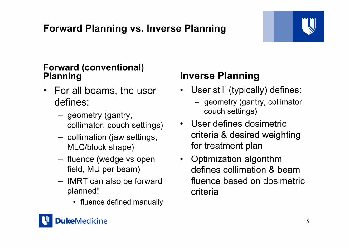
Forward (conventional) Planning •  For all beams, the user

defines: –  geometry (gantry,

collimator, couch settings) –  collimation (jaw settings,

MLC/block shape) –  fluence (wedge vs open

field, MU per beam) –  IMRT can also be forward

planned! •  fluence defined manually

Inverse Planning •  User still (typically) defines:

–  geometry (gantry, collimator, couch settings)

•  User defines dosimetric criteria & desired weighting for treatment plan

•  Optimization algorithm defines collimation & beam fluence based on dosimetric criteria

8

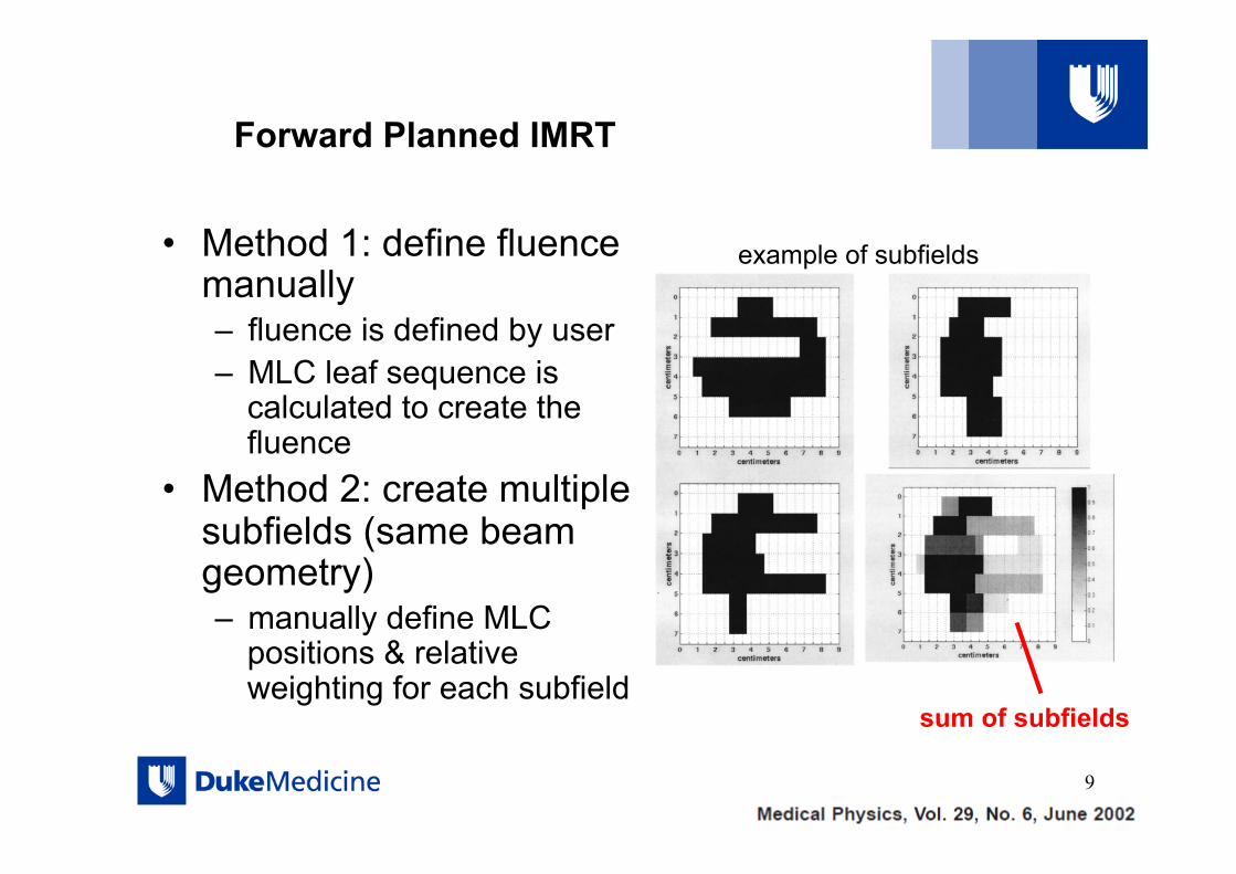
Forward Planned IMRT

•  Method 1: define fluence manually –  fluence is defined by user –  MLC leaf sequence is

calculated to create the fluence

•  Method 2: create multiple subfields (same beam geometry) –  manually define MLC

positions & relative weighting for each subfield

9

example of subfields

sum of subfields

Inverse Planned IMRT: Optimization

•  Beam fluence is divided into “beamlets” •  Beamlet dimensions:

–  0.2-1.0cm along leaf motion direction –  leaf width in cross-leaf direction

•  Only optimize beamlets that traverse the target (plus small margin)

10

Inverse Planning: Optimization

•  Dose in voxel i is given by

where wj is the intensity of the jth beamlet, i=1, …I is the number of dose voxels and where the sum is carried out from j = 1,..J, the total number of beamlets. We want to find wj values •  The quantity aij is the dose deposited in the ith voxel by

the jth beamlet for unit fluence

11

beamlet j

voxel iD a wi ijj

J

j==∑1

Inverse Planning: Optimization

•  Dose in any voxel can be written as a linear combination of beamlet intensities.

•  First step is to calculate the contribution to dose per unit fluence in each voxel due to each beamlet

•  Dose calculation is done “up front” rather than during optimization

•  (The same process is carried out regardless of dose calculation algorithm)

12

Inverse Planning: Optimization

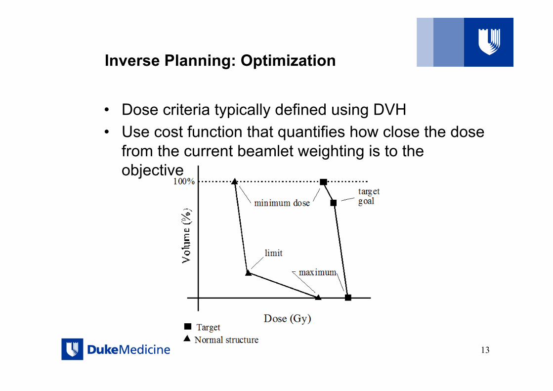
•  Dose criteria typically defined using DVH •  Use cost function that quantifies how close the dose

from the current beamlet weighting is to the objective

13

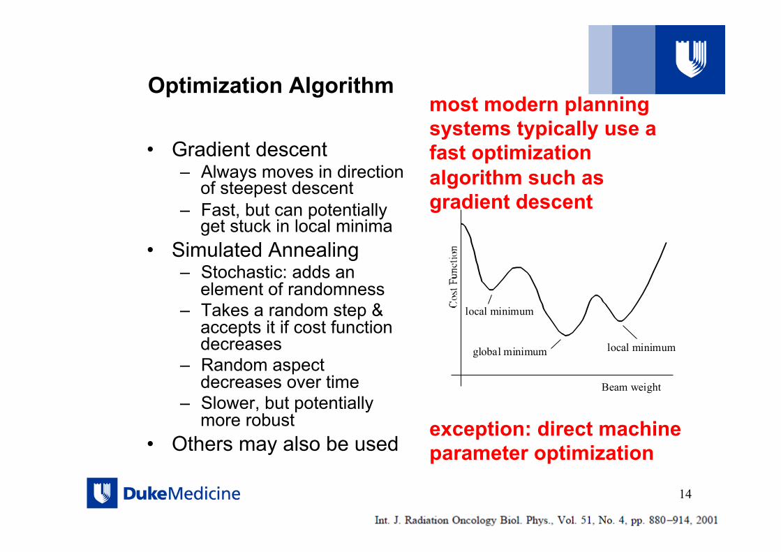
Optimization Algorithm

•  Gradient descent –  Always moves in direction

of steepest descent –  Fast, but can potentially

get stuck in local minima •  Simulated Annealing

–  Stochastic: adds an element of randomness

–  Takes a random step & accepts it if cost function decreases

–  Random aspect decreases over time

–  Slower, but potentially more robust

•  Others may also be used

local minimum

local minimumglobal minimum

Beam weight

14

most modern planning systems typically use a fast optimization algorithm such as gradient descent

exception: direct machine parameter optimization

How to deliver the fluence?

•  Physical Compensators •  MLC motion

–  leaf sequence to match ideal fluence –  Direct Machine Parameter Optimization (Direct Aperture

Optimization) •  skip fluence step! Or in other words: the leaf sequence is

optimized and comes first; the fluence can be calculated from the leaf sequence.

15

IMRT Methods: Physical Compensator

16

Primary Fluence

Compensator

Modulated Fluence

IMRT Methods: Physical Compensators

17

reusable tin granules & compensator box

disposable styrofoam mold

IMRT Methods: Physics Compensators

Advantage: simple implementation •  no need for MLCs •  static delivery •  no interplay

between intensity modulation and organ motion

Disadvantage: lack of automation •  each field requires a

custom compensator

•  need to enter room per field

•  Limited modulation

18

IMRT Methods: Physical Compensators

•  Max compensator thickness ~5cm

•  tin: –  100% - 38% 6X –  100% - 45% 15X

•  tungsten powder: –  100% - 18% 6X –  100% - 20% 15X

19

actual fluence vs ideal fluence

IMRT Methods: Physical Compensators

Ideal Compensator Criteria: •  large range of

intensity modulation magnitude

•  intensity modulation of high spatial resolution

•  not hazardous during fabrication

•  easy to form to & retain shape

•  low material cost •  environmentally

friendly

20

MLC Based IMRT:

•  Leaf Sequencing Algorithm: –  “Inverse optimization” derives “fluence” per field –  “Leaf sequencing algorithm” determines an MLC motion to

deliver the fluence –  There will likely be some difference between the “optimal”

and “actual” fluence

•  Alternative Strategy: Direct Machine Parameter Optimization (DMPO) or Direct Aperture Optimization (DAO) –  Actual machine parameters (leaf positions, etc.) optimized

directly –  Advantage: what you see (at optimization) is what you get –  Disadvantage: potentially slower optimization

21

Leaf Sequencing Algorithm:

•  There are many solutions to create a desired fluence –  some idealized intensity patterns may not be deliverable –  leaf transmission sets a lower bound on intensity

•  Must account for limitations in leaf position & leaf speed •  Algorithms may attempt to minimize:

–  # segments –  MU –  leaf travel or delivery time –  tongue & groove effect

•  The difference between actual & desired intensity may be greater for complicated intensities; these also lead to more complicated leaf sequences, increased MU, and / or # segments –  because of this often the inverse optimization may smooth the fluence

or include a penalty for complex fluences

22

Leaf Sequencing Algorithm:

•  The final dose calculation from the treatment planning system may be based on either the ideal fluence OR the final fluence from the leaf sequence –  important to know which is being reported, since a dose

degradation may be expected between these two –  greater degradation may be expected for more complicated

fluence patterns

•  Dose calculation during optimization may be simplified to increase speed

23

IMRT Methods: Step & Shoot (static MLC)

24

IMRT leaf sequencing

25

leaves may “close in” with each segment

or “sweep across” the field (this is the method always used for dynamic MLC IMRT)

same fluence can be delivered with both methods

IMRT Methods: Sweeping Leaves for dynamic MLC

26

desired fluence to create a single direction of travel areas of decreasing fluence are offset

remove incontinuities

27

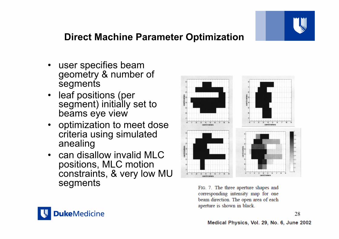
Direct Machine Parameter Optimization

•  user specifies beam geometry & number of segments

•  leaf positions (per segment) initially set to beams eye view

•  optimization to meet dose criteria using simulated anealing

•  can disallow invalid MLC positions, MLC motion constraints, & very low MU segments

28

IMRT Methods: Step & Shoot (static MLC)

29

fluence from sum of all subfields (or segments)

Segments (subfields) may be defined by forward planning, or inverse planning. Segments from inverse plans may be derived via a leaf sequence algorithm, or directly from optimization (DMPO)!

IMRT ‘step and shoot’ and sliding window

30

IMRT Treatment Planning Process

31

Simulation

Contouring (MD & Dosimetrist)

Prescription & Dosimetric Constraints

(MD)

Set Beam Geometry

Select Optimization Criteria: target & organ constraints & weights

Optimize Fluence

Calculate MLC motion (leaf sequence)

Calculate Dose

IMRT: Beam Setup

•  Typically 7-12 equi-spaced beams

•  Isocenter placed near center of PTV

32

IMRT Beam Setup

•  Lateral beams: still avoid going through shoulders

33

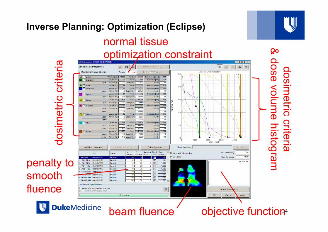
Inverse Planning: Optimization (Eclipse)

dosi

met

ric c

riter

ia dosim

etric criteria &

dose volume histogram

beam fluence objective function 34

penalty to smooth fluence

normal tissue optimization constraint

3D IMRT

3D IMRT

35

3D vs IMRT

3D IMRT

3D IMRT

36

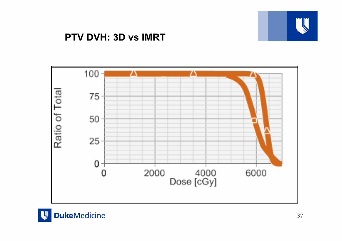
PTV DVH: 3D vs IMRT

37

Spinal Cord DVH: 3D vs IMRT

38

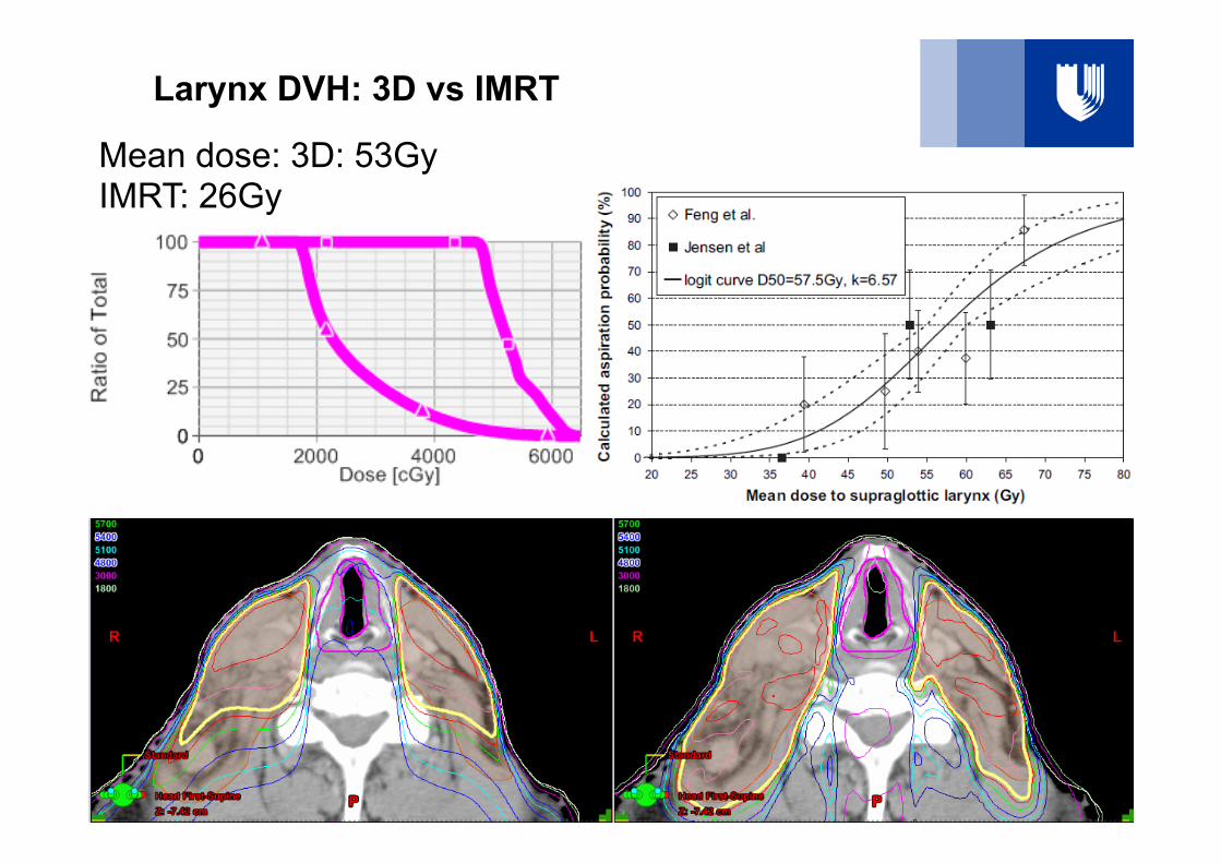
Larynx DVH: 3D vs IMRT

39

Mean dose: 3D: 53Gy IMRT: 26Gy

Parotid DVH: 3D vs IMRT

40

41

Intensity Map for an IMRT beam superimposed on patient DRR (left) and reflected in hair loss on patient scalp (right)

4F conformal plan

5F IMRT

Axial views

Ant

Lt Rt

Post

What can IMRT achieve in prostate Tx ?

4F conformal plan 5F IMRT plan

What can IMRT achieve in prostate Tx ?

Sup

Ant

Inf

Post

Saggital views

IMRT vs conformal DVH

Rectal wall

Bladder

Cl-PTV

Cl-PTV no rect

Dashed=4F conformal, solid = IMRT

In IMRT plans typically ..: - •  PTV less homogenous •  Modest sparing OAR regions that overlap with the PTV • Significant sparing of OARs that don’t overlap with the PTV.

Some comments on IMRT

•  Better conformity -> may be easier to miss the target ?! –  Potentially a significant problem –  First get the margins correct, then implement IMRT

•  Beam selection can be non-intuitive •  Tendency to use more beams not less ! •  Typical MUs for an IMRT plan are 3-5 times higher

–  Tendency to use lower energy (reduce neutron)

•  Tendency to ‘over-stress’ IMRT planning –  Give the optimization a consistent set of objectives –  Avoid extreme weighting etc

45

Summary of IMRT

Advantages •  Ability to produce

remarkably conformal dose distributions

•  Dose escalation (improvement in local control)

•  Decreased dose to surrounding tissues (reduction in complications)

Disadvantages •  Planning is labor intensive •  Extended delivery time

(typically) •  Danger of being too

conformal •  Generally more

inhomogeneous dose distribution

•  Increased MU→ increased whole body dose & increased room shielding

46

References

•  INTENSITY-MODULATED RADIOTHERAPY: CURRENT STATUS AND ISSUES OF INTEREST, Int. J. Radiation Oncology Biol. Phys., Vol. 51, No. 4, pp. 880–914, 2001

•  Optimized Planning Using Physical Objectives and Constraints, Thomas Bortfield, Seminars in Radiation Oncology, Vol 9, No 1 (January), 1999:pfl 20-34

•  Image Guided Radiation Therapy (IGRT) Technologies for Radiation Therapy Localization and Delivery, Int J Radiation Oncol Biol Phys, Vol. 87, No. 1, pp. 33e45, 2013

•  Image-guided radiotherapy: rationale, benefits, and limitations, Lancet Oncol 2006; 7: 848–58

•  Planning in the IGRT Context: Closing the Loop, Semin Radiat Oncol 17:268-277

47

Thank You!

48