Intelligent Fault Diagnosis & Prognosis - UTA talks/Metrocon 07 intel diag and prog... · New Business Models for ... Periodic, whether needed or not Run-to-Failure No maintenance

Automation & Robotics Research Institute (ARRI)The University of Texas at Arlington

F.L. Lewis, IEEE FellowMoncrief-O’Donnell Endowed Chair

Head, Controls & Sensors Group

http://ARRI.uta.edu/[email protected]

Intelligent Fault Diagnosis & Prognosis

John Wiley, New York, 2006 John Wiley, New York, 2003

Why Intelligent Diagnostics & Prognostics?

Diagnostics

Intelligent Decision Making

Prognostics

Condition-Based Maintenance

Signal Processing

Machinery Monitoring using Wireless Sensor Networks

Outline

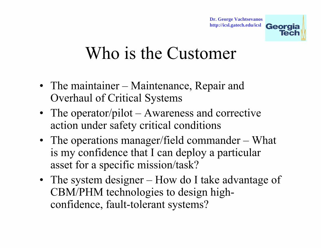
Who is the Customer

• The maintainer – Maintenance, Repair and Overhaul of Critical Systems

• The operator/pilot – Awareness and corrective action under safety critical conditions

• The operations manager/field commander – What is my confidence that I can deploy a particular asset for a specific mission/task?

• The system designer – How do I take advantage of CBM/PHM technologies to design high-confidence, fault-tolerant systems?

Dr. George Vachtsevanoshttp://icsl.gatech.edu/icsl

New Business Models for Machinery MaintenanceOriginal Equipment Manufacturer Becomes the Service Provider

Integrate Manufacturing, Service, and MaintenanceLifetime Machine Service ContractGuaranteed Up-Time for UserGuaranteed Lifetime Revenue Stream for OEM

• Internet-Based E-Maintenance• Integrate Internet with Machine On-Board Diagnostics• Centralized Service Scheduling and Dispatching• Reduced Service Costs

Subcontracted Maintenance Service ProvidersMSP provides and maintains the wireless sensor networkMSP monitors equipment, schedules & provides maintenanceLike current Security Systems- Brinks, etc.

Dr. Jay Lee

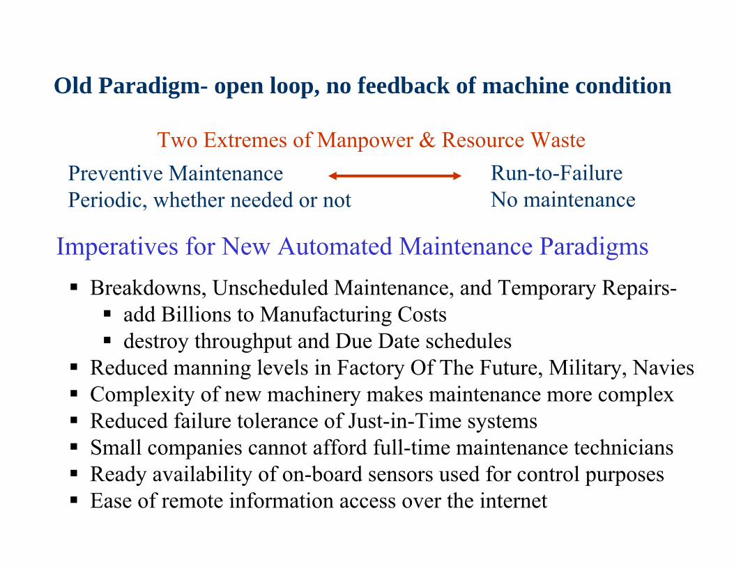
Imperatives for New Automated Maintenance ParadigmsBreakdowns, Unscheduled Maintenance, and Temporary Repairs-

add Billions to Manufacturing Costsdestroy throughput and Due Date schedules

Reduced manning levels in Factory Of The Future, Military, NaviesComplexity of new machinery makes maintenance more complexReduced failure tolerance of Just-in-Time systemsSmall companies cannot afford full-time maintenance techniciansReady availability of on-board sensors used for control purposesEase of remote information access over the internet

Old Paradigm- open loop, no feedback of machine condition

Preventive MaintenancePeriodic, whether needed or not

Run-to-FailureNo maintenance

Two Extremes of Manpower & Resource Waste

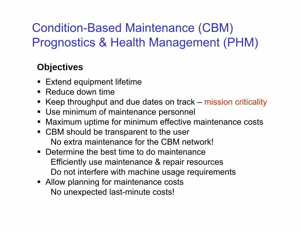
ObjectivesExtend equipment lifetimeReduce down timeKeep throughput and due dates on track – mission criticalityUse minimum of maintenance personnelMaximum uptime for minimum effective maintenance costsCBM should be transparent to the user

No extra maintenance for the CBM network!Determine the best time to do maintenance

Efficiently use maintenance & repair resourcesDo not interfere with machine usage requirements

Allow planning for maintenance costsNo unexpected last-minute costs!

Condition-Based Maintenance (CBM)Prognostics & Health Management (PHM)

CBM+: Maintenance-CentricLogistics Support for the Future


www.MIMOSA.orgMachine User Group- CBM Data

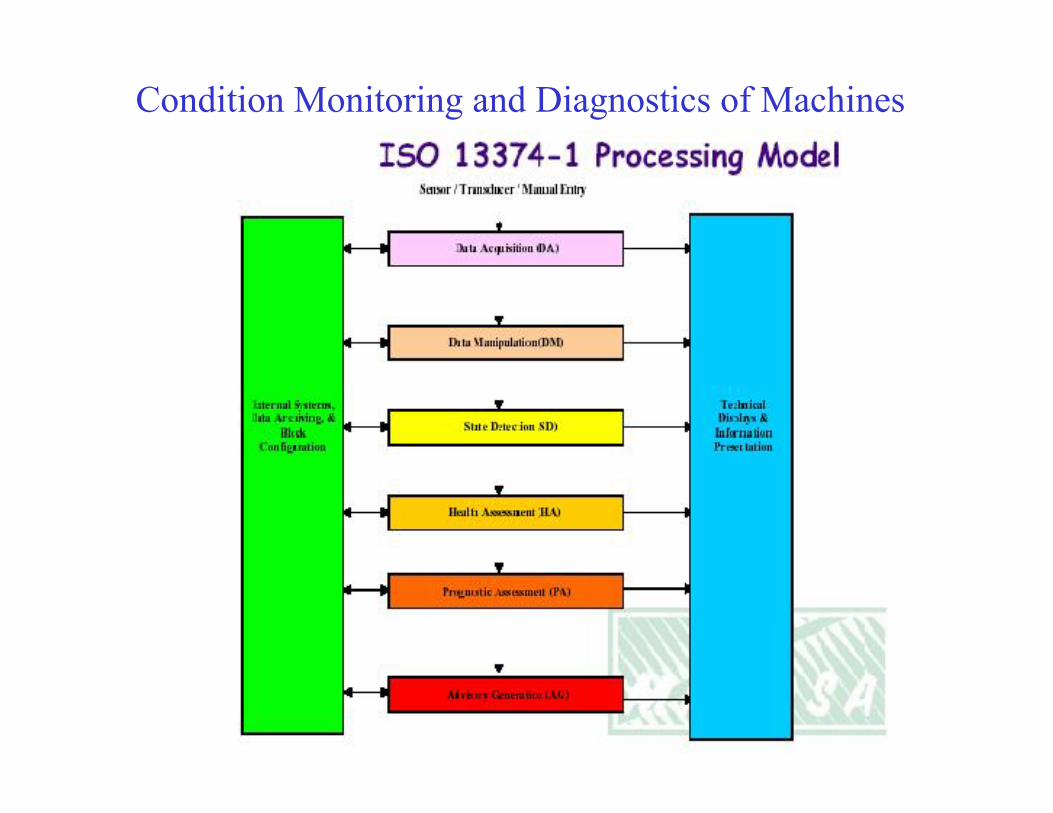
Condition Monitoring and Diagnostics of Machines

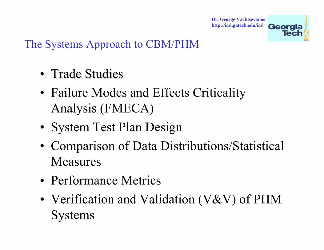
The Systems Approach to CBM/PHM

•• Trade StudiesTrade Studies• Failure Modes and Effects Criticality

Analysis (FMECA)• System Test Plan Design• Comparison of Data Distributions/Statistical

Measures• Performance Metrics• Verification and Validation (V&V) of PHM

Systems


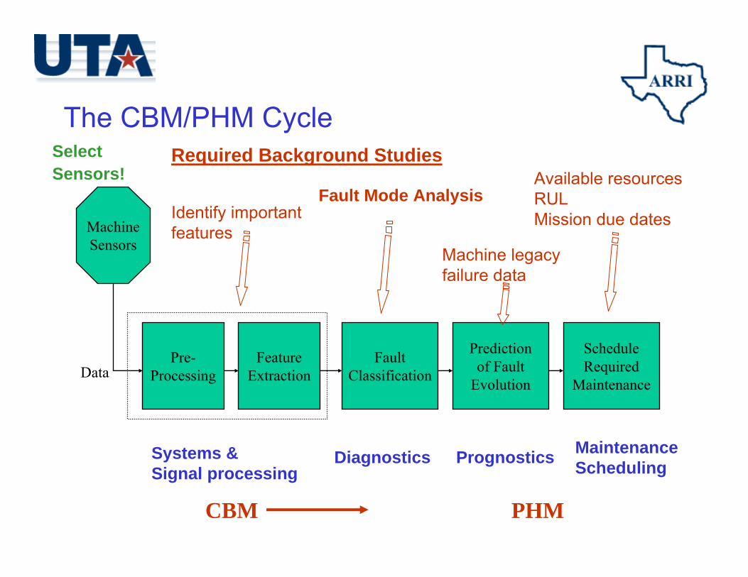
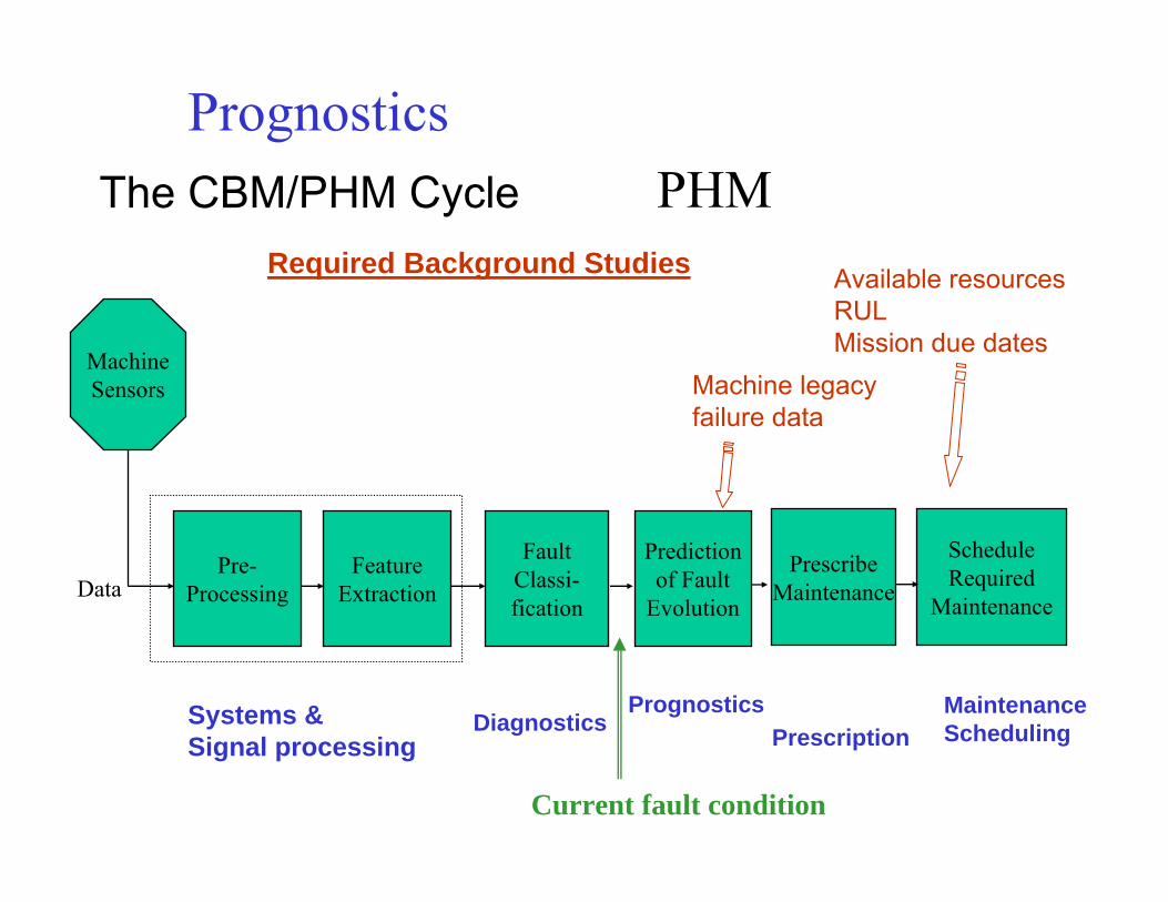
The CBM/PHM Cycle

MachineSensors

Pre-Processing

FeatureExtraction

FaultClassification

Predictionof Fault

EvolutionData

ScheduleRequired

Maintenance

Systems &Signal processing

Diagnostics Prognostics MaintenanceScheduling

Identify importantfeatures

Fault Mode Analysis

Machine legacy failure data

Available resourcesRULMission due dates

Required Background Studies

PHMCBM

SelectSensors!

Off Line- Background Studies, Fault Mode AnalysisOn Line- Perform real-time Fault Monitoring & Diagnosis

Two Phases of CBM Diagnostics

Three Stages of CBM/PHM

DiagnosticsPrognosticsMaintenance Scheduling

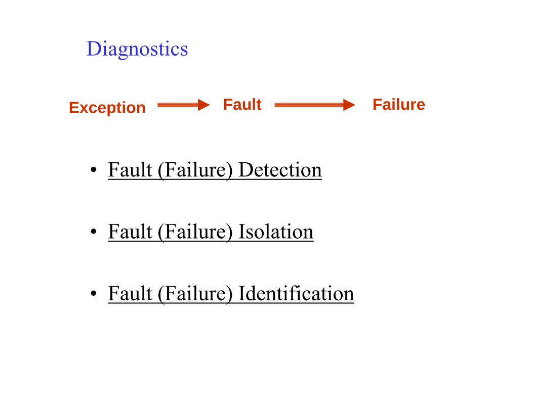
Diagnostics

• Fault (Failure) Detection

• Fault (Failure) Isolation

• Fault (Failure) Identification

Exception Fault Failure

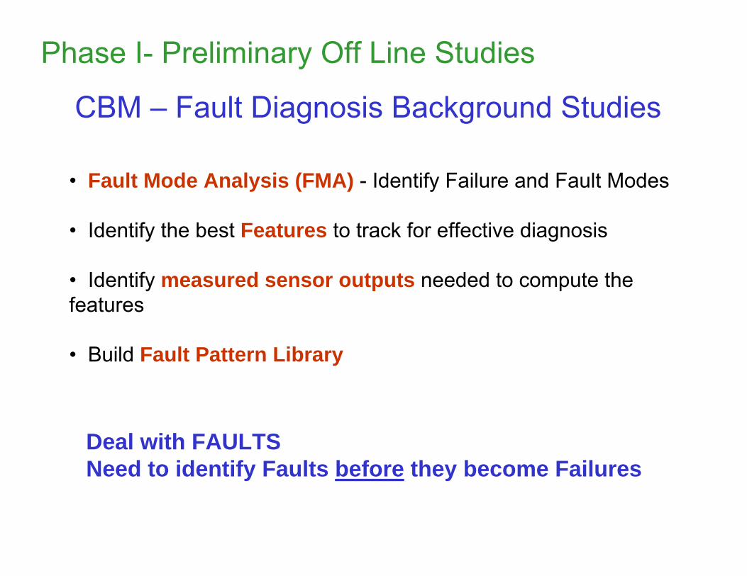
CBM – Fault Diagnosis Background Studies

• Fault Mode Analysis (FMA) - Identify Failure and Fault Modes

• Identify the best Features to track for effective diagnosis

• Identify measured sensor outputs needed to compute the features

• Build Fault Pattern Library

Deal with FAULTSNeed to identify Faults before they become Failures

Phase I- Preliminary Off Line Studies

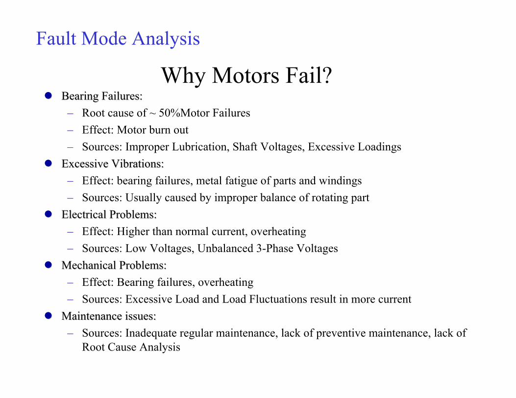
Why Motors Fail?Bearing Failures:Bearing Failures:– Root cause of ~ 50%Motor Failures– Effect: Motor burn out– Sources: Improper Lubrication, Shaft Voltages, Excessive Loadings

Excessive Vibrations:Excessive Vibrations:– Effect: bearing failures, metal fatigue of parts and windings– Sources: Usually caused by improper balance of rotating part

Electrical Problems:Electrical Problems:– Effect: Higher than normal current, overheating– Sources: Low Voltages, Unbalanced 3-Phase Voltages

Mechanical Problems:Mechanical Problems:– Effect: Bearing failures, overheating– Sources: Excessive Load and Load Fluctuations result in more current

Maintenance issues:Maintenance issues:– Sources: Inadequate regular maintenance, lack of preventive maintenance, lack of

Root Cause Analysis

Fault Mode Analysis

Compressor Pre-rotation Vane

Condenser

Evaporator

•Compressor Stall & Surge•Shaft Seal Leakage•Oil Level High/Low•Aux. Pump Fail•Oil Cooler Fail•PRV/VGD Mechanical Failure

•Condenser Tube Fouling•Condenser Water Control Valve Failure•Tube Leakage•Decreased Sea Water Flow

•Target Flow Meter Failure•Decreased Chilled Water Flow•Evaporator Tube Freezing

•Non Condensable Gas in Refrigerant•Contaminated Refrigerant•Refrigerant Charge High•Refrigerant Charge Low

•SW in/out temp.•SW flow•Cond. press.•Cond. PD press.•Cond. liquid out temp.

•Comp. suct. press./temp.•Comp. disch. press./temp.•Comp. oil press./flow (at required points)•Comp. bearing oil temp•Comp. suct. super-heat•Shaft seal interface temp.•PRV Position

•Liquid line temp.•(Refrigerant weight)

•CW in/out temp./flow•Eva. temp./press.•Eva. PD press.

Ex. Ex. -- Navy Centrifugal Chiller Failure ModesNavy Centrifugal Chiller Failure Modes

Fault Mode AnalysisDr. George Vachtsevanoshttp://icsl.gatech.edu/icsl

Fault Mode: Refrigerant Charge Low

Symptoms: 1. Low Evaporator Liquid Temperature2. Low Evaporator Suction pressure3. Increasing difference (D-ELT-CWDT) between Chilled Water

Discharge Temperature and Evaporator Liquid Temperature

Sensors: 1. Evaporator Liquid Temperature (ELT)2. Evaporator Suction Pressure (ESP)3. Chilled Water Discharge Temperature (CWDT)

Failure Modes and Effects Criticality Analysis

Failure Modes and Effects Criticality Analysis

New systematic approach based on fuzzy Petri networks and efficient search techniques to define failure effect – root cause relationships

Large LeakDetected (0.9)

Ok (0.9)Not ok (0.1)

CheckPressure Meter

CheckVacuum Pump

Check forOverheating

Check forDirty Fluid

(0.81)

Ok (0.9)

Ok (0.8)

Ok (0.1)

Not ok (0.1)

Not ok (0.2)

Not ok (0.9)

Large Leak While Meter Readingis Correct (0.81)


Helicopter Fault Tree

HelicopterFailure

MotorFailures

ActuatorFailures

PowerFailures

SensorFailures

Computer SystemFailures

Main RotorFailures

Tail RotorFailures


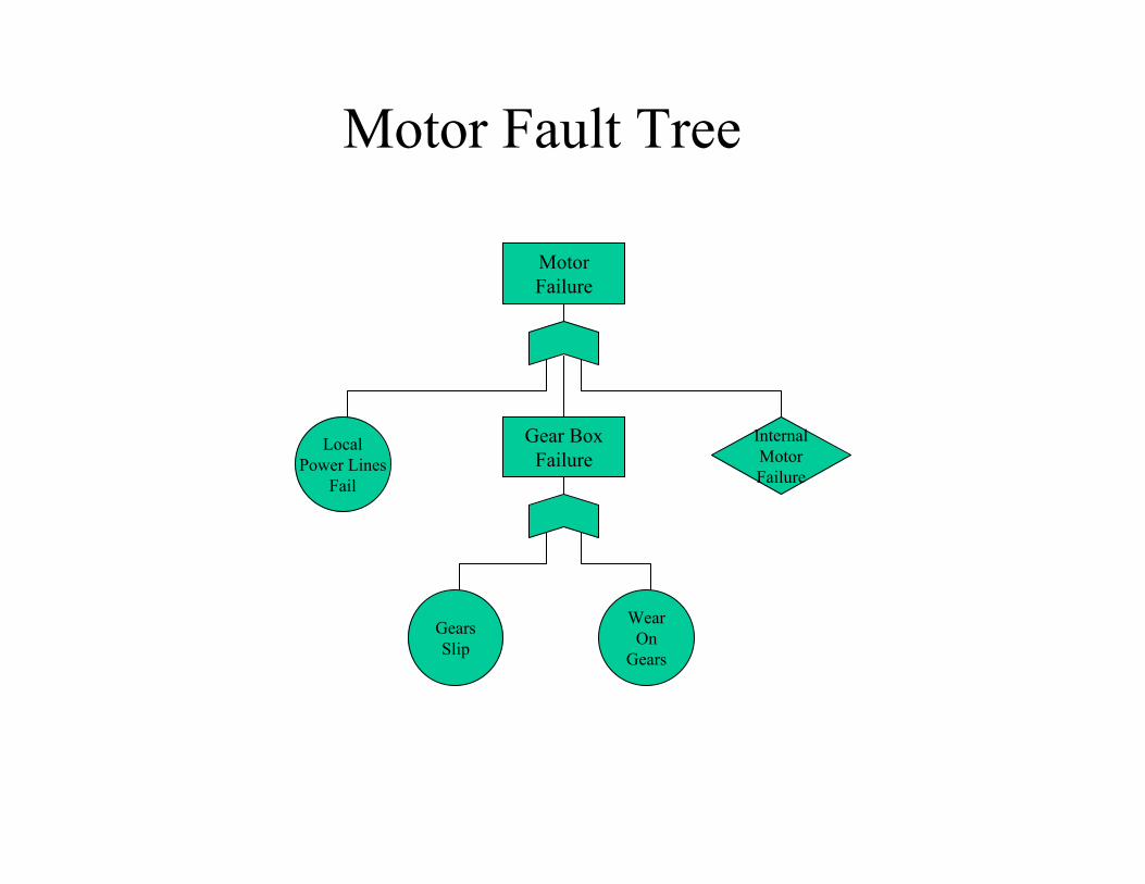
Motor Fault Tree

MotorFailure

Gear BoxFailure

InternalMotorFailure

LocalPower Lines

Fail

GearsSlip

WearOn

Gears

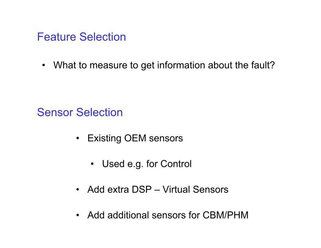
Sensor Selection

• Existing OEM sensors

• Used e.g. for Control

• Add extra DSP – Virtual Sensors

• Add additional sensors for CBM/PHM

Feature Selection

• What to measure to get information about the fault?

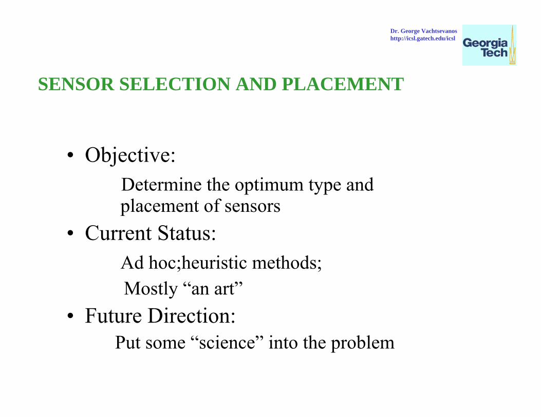
SENSOR SELECTION AND PLACEMENT

• Objective: Determine the optimum type and placement of sensors

• Current Status:Ad hoc;heuristic methods;Mostly “an art”

• Future Direction: Put some “science” into the problem


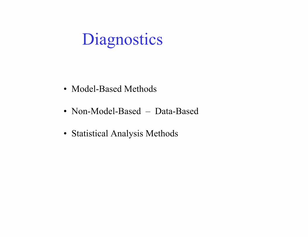
Diagnostics

• Model-Based Methods

• Non-Model-Based – Data-Based

• Statistical Analysis Methods

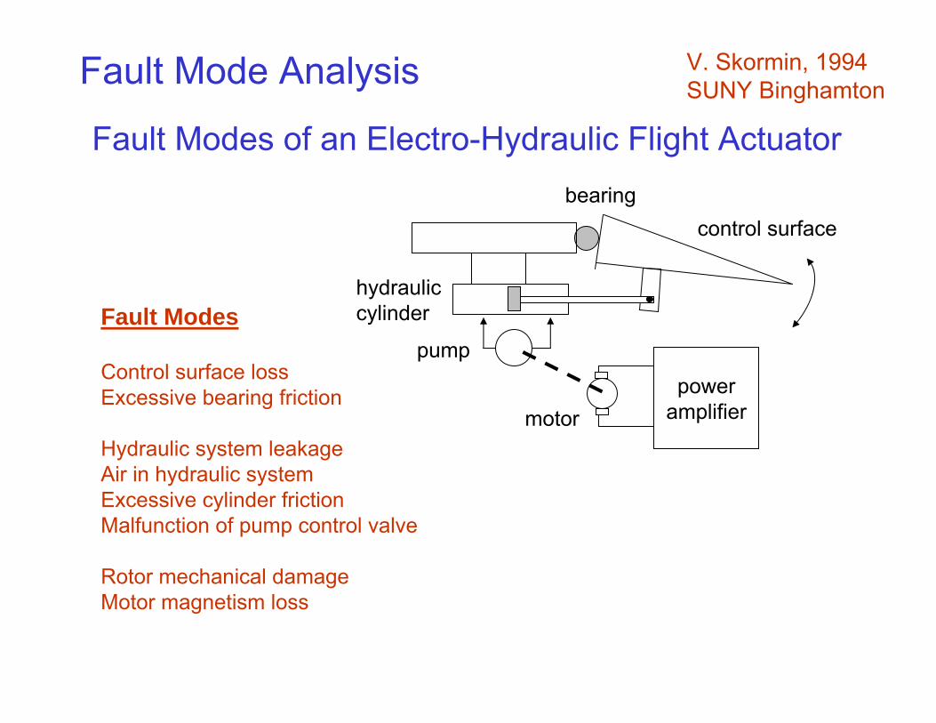
Fault Modes of an Electro-Hydraulic Flight Actuator

V. Skormin, 1994SUNY Binghamton

bearingcontrol surface

hydrauliccylinder

pump

poweramplifier

Fault Modes

Control surface lossExcessive bearing friction

Hydraulic system leakageAir in hydraulic systemExcessive cylinder frictionMalfunction of pump control valve

Rotor mechanical damageMotor magnetism loss

motor

Fault Mode Analysis

Use Physics of Failure and Failure Models to select failure features to include in feature vectors

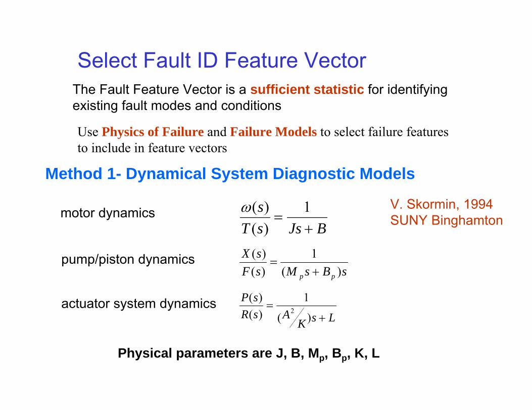
Select Fault ID Feature Vector

Method 1- Dynamical System Diagnostic Models

The Fault Feature Vector is a sufficient statistic for identifying existing fault modes and conditions

BJssTs

+=

1)()(ωmotor dynamics

sBsMsFsX

pp )(1

)()(

+=pump/piston dynamics

LsKAsR

sP

+=

)(

1)()(

2actuator system dynamics

Physical parameters are J, B, Mp, Bp, K, L


Select Feature VectorRelate physical parameters J, B, Mp, Bp, K, L to fault modes

Get expert opinion (from manufacturer or from user group)Get actual fault/failure legacy data from recorded machine historiesOr run system testbed under induced faults

Result -

Etc.Etc.

THEN (fault is air in hydraulic system)IF (actuator stiffness K is small)AND (piston damping coeff. Bp is small)

THEN (fault is excess cylinder friction)IF (motor damping coeff. B is large)AND (piston damping coeff. Bp is large)

THEN (fault is hydraulic system leakage)IF (leakage coeff. L is large)Fault ModeCondition

Therefore, select the physical parameters as the feature vectorT

pp LKBMBJt ][)( =φ


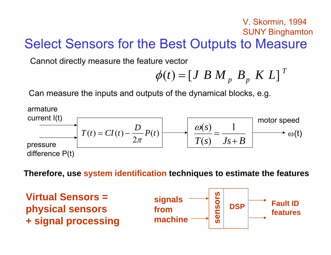
Select Sensors for the Best Outputs to Measure


Tpp LKBMBJt ][)( =φ

Cannot directly measure the feature vector

Can measure the inputs and outputs of the dynamical blocks, e.g.

BJssTs

+=

1)()(ω

)(2

)()( tPDtCItTπ

−= ω(t)motor speed

armaturecurrent I(t)

pressuredifference P(t)

Therefore, use system identification techniques to estimate the features

Virtual Sensors = physical sensors + signal processing se

nsor

sDSP

signals from machine

Fault IDfeatures

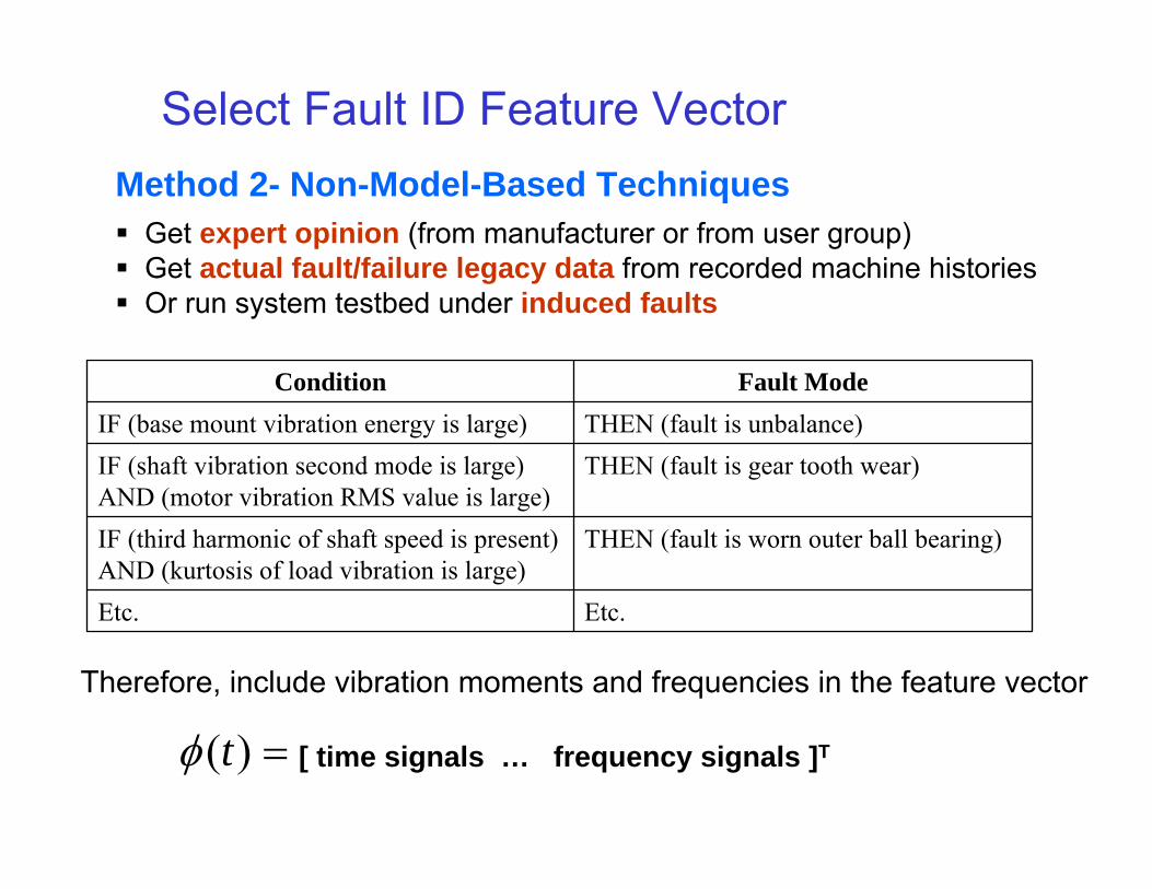
Method 2- Non-Model-Based Techniques


Etc.Etc.

THEN (fault is worn outer ball bearing)IF (third harmonic of shaft speed is present)AND (kurtosis of load vibration is large)

THEN (fault is gear tooth wear)IF (shaft vibration second mode is large)AND (motor vibration RMS value is large)

THEN (fault is unbalance)IF (base mount vibration energy is large)Fault ModeCondition

Therefore, include vibration moments and frequencies in the feature vector

=)(tφ [ time signals … frequency signals ]T

Get expert opinion (from manufacturer or from user group)Get actual fault/failure legacy data from recorded machine historiesOr run system testbed under induced faults

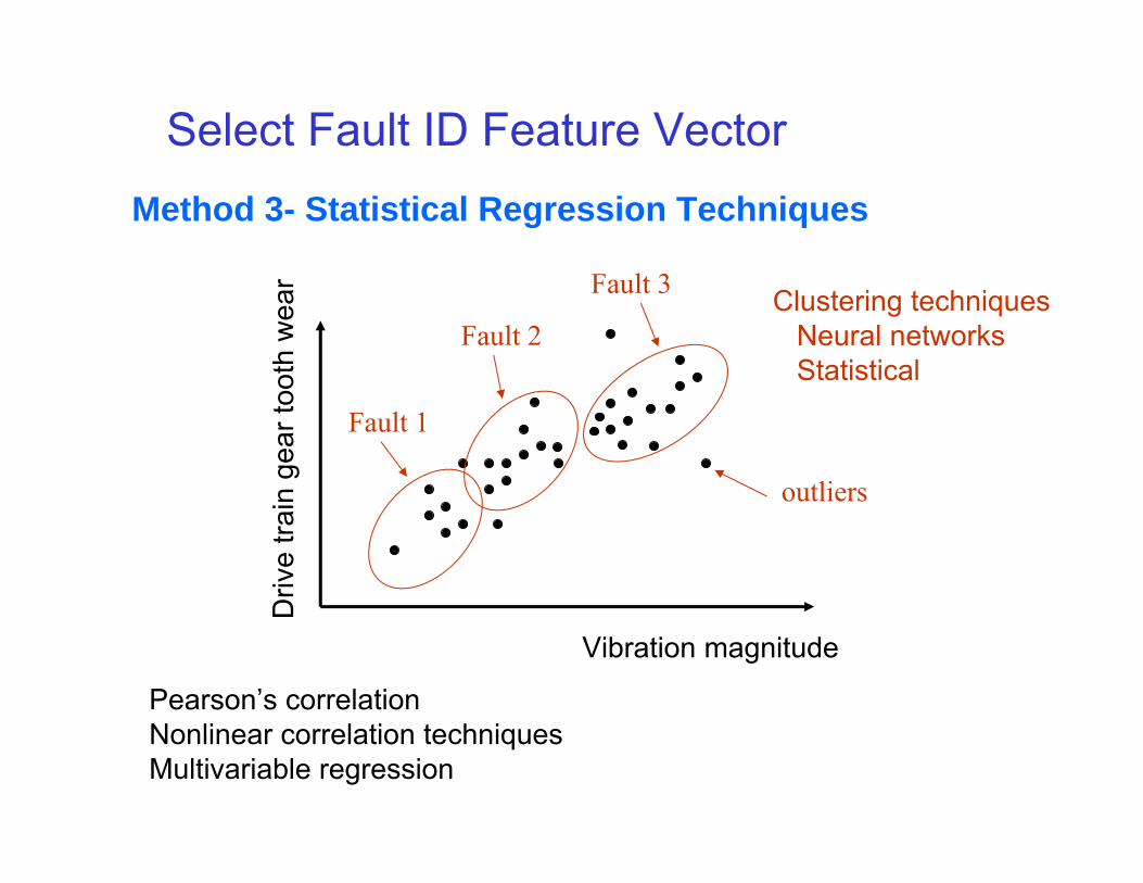
Method 3- Statistical Regression Techniques


Vibration magnitude

Driv

e tra

in g

ear t

ooth

wea

r

Pearson’s correlationNonlinear correlation techniquesMultivariable regression

Clustering techniquesNeural networksStatistical

Fault 1

Fault 2

Fault 3

outliers

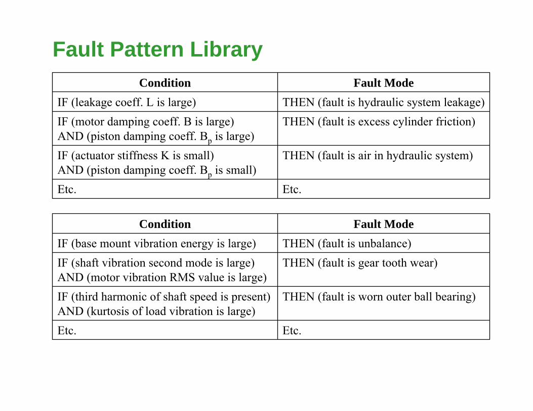
Etc.Etc.

THEN (fault is air in hydraulic system)IF (actuator stiffness K is small)AND (piston damping coeff. Bp is small)

THEN (fault is excess cylinder friction)IF (motor damping coeff. B is large)AND (piston damping coeff. Bp is large)

THEN (fault is hydraulic system leakage)IF (leakage coeff. L is large)Fault ModeCondition

Fault Pattern Library

Etc.Etc.

THEN (fault is worn outer ball bearing)IF (third harmonic of shaft speed is present)AND (kurtosis of load vibration is large)

THEN (fault is gear tooth wear)IF (shaft vibration second mode is large)AND (motor vibration RMS value is large)

THEN (fault is unbalance)IF (base mount vibration energy is large)Fault ModeCondition

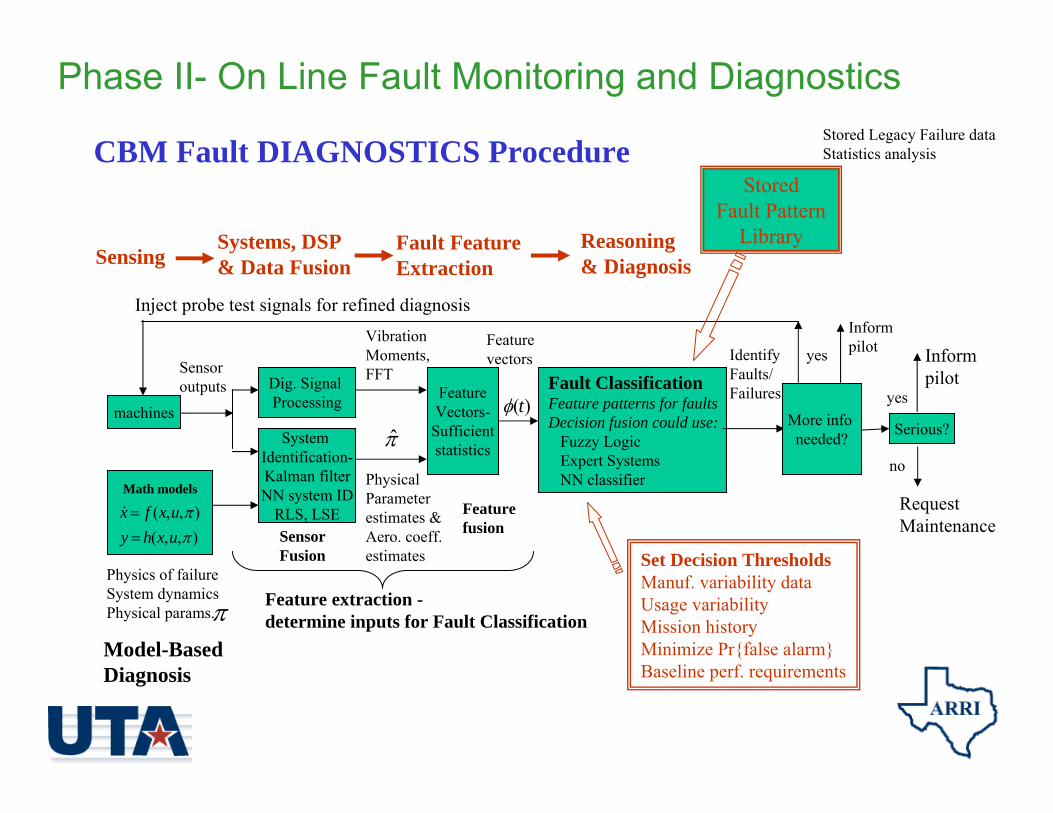
CBM Fault DIAGNOSTICS Procedure

machines

Math models

),,(),,(

ππ

uxhyuxfx

==

System Identification-Kalman filterNN system ID

RLS, LSE

Dig. Signal Processing

PhysicalParameterestimates &Aero. coeff.estimates

π̂

Sensoroutputs

VibrationMoments, FFT

FeatureVectors-

Sufficientstatistics

)(tφFault ClassificationFeature patterns for faultsDecision fusion could use:

Fuzzy LogicExpert SystemsNN classifier

Stored Legacy Failure dataStatistics analysis

Feature extraction -determine inputs for Fault Classification

Physics of failureSystem dynamicsPhysical params.

Identify Faults/Failures

More info needed?

Inject probe test signals for refined diagnosisInformpilotyes

π

Serious?

Informpilot

yes

SensingFault Feature Extraction

Reasoning& Diagnosis

Systems, DSP& Data Fusion

SensorFusion

Featurevectors

Featurefusion

StoredFault Pattern

Library

Model-BasedDiagnosis

Set Decision ThresholdsManuf. variability dataUsage variabilityMission historyMinimize Pr{false alarm}Baseline perf. requirements

Phase II- On Line Fault Monitoring and Diagnostics

no

Request Maintenance

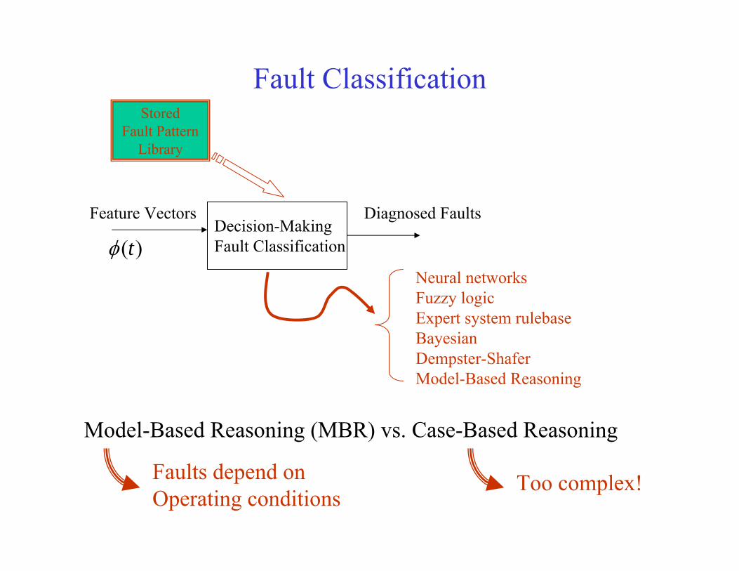
Fault Classification

Decision-MakingFault Classification

StoredFault Pattern

Library

Feature Vectors

)(tφ

Diagnosed Faults

Model-Based Reasoning (MBR) vs. Case-Based Reasoning

Too complex!Faults depend on Operating conditions

Neural networksFuzzy logicExpert system rulebaseBayesianDempster-ShaferModel-Based Reasoning

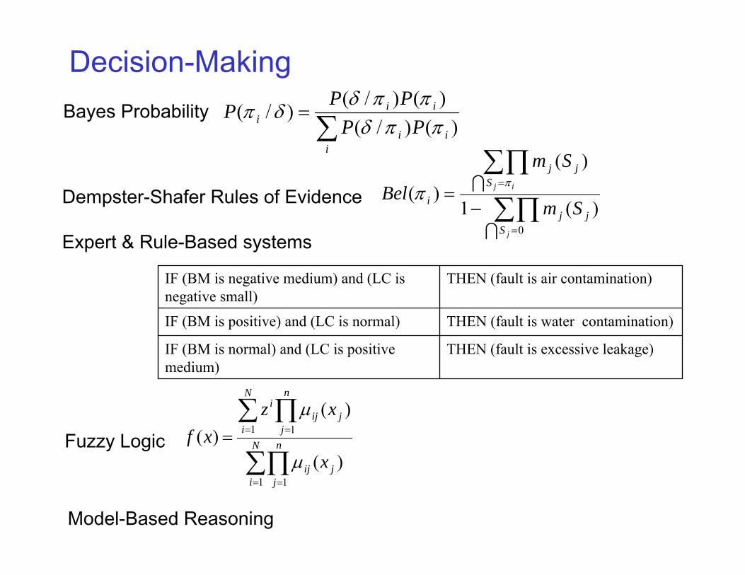
Decision-Making

∑∏

∑ ∏

= =

= == N

i

n

jjij

N

i

n

jjij

i

x

xzxf

1 1

1 1

)(

)()(

μ

μ

THEN (fault is excessive leakage)IF (BM is normal) and (LC is positive medium)

THEN (fault is water contamination)IF (BM is positive) and (LC is normal)

THEN (fault is air contamination)IF (BM is negative medium) and (LC is negative small)

∑=

iii

iii PP

PPP

)()/()()/(

)/(ππδ

ππδδπ

∑∏

∑∏

=

=

−=

∩

∩

0

)(1

)(

)(

j

ij

Sjj

Sjj

i Sm

Sm

Belπ

π

Bayes Probability

Dempster-Shafer Rules of Evidence

Expert & Rule-Based systems

Fuzzy Logic

Model-Based Reasoning

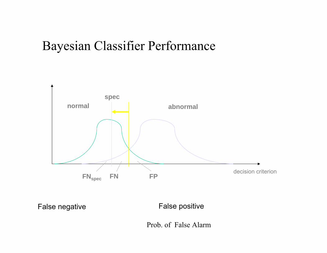
Bayesian Classifier Performance

normal abnormal

FN FP

spec

FNspecdecision criterion

False positiveFalse negative

Prob. of False Alarm

∑

∑

∅=∩

=∩

−=⊗

ji

ji

BAji

CBAji

BmAm

BmAmCmm

)()(1

)()()(

21

21

21

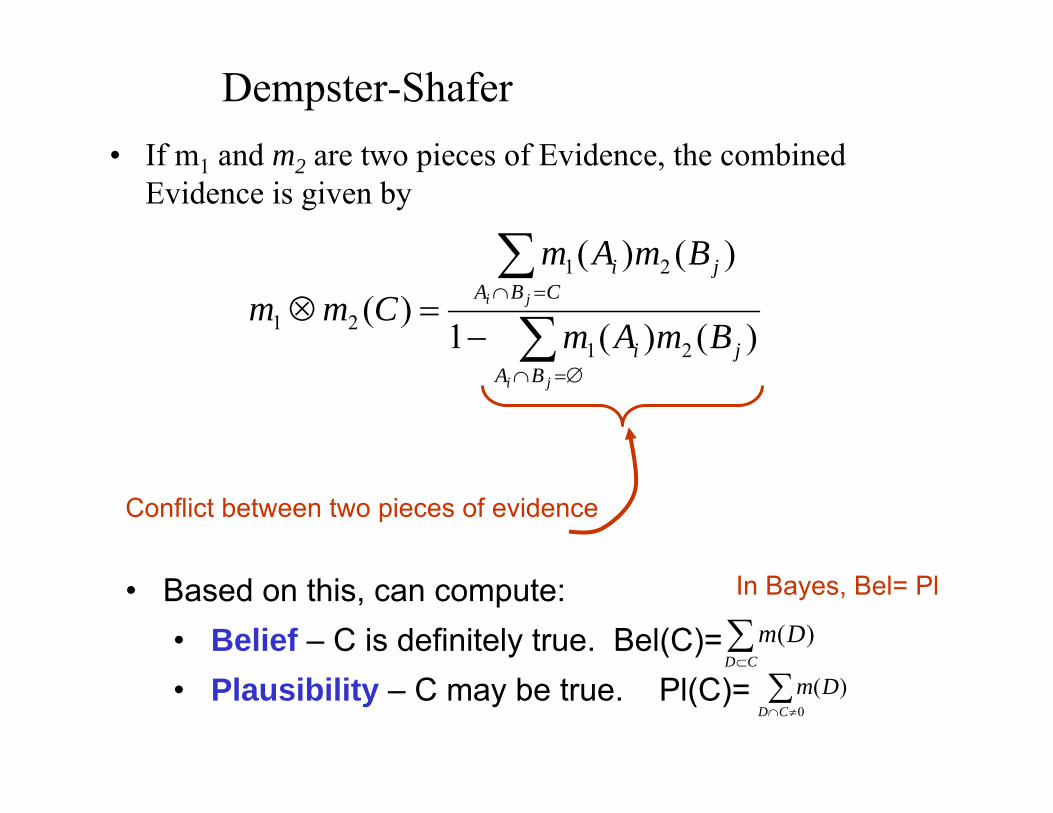
Dempster-Shafer• If m1 and m2 are two pieces of Evidence, the combined

Evidence is given by

Conflict between two pieces of evidence

• Based on this, can compute:• Belief – C is definitely true. Bel(C)= • Plausibility – C may be true. Pl(C)=

∑⊂CD

Dm )(

∑≠∩ 0

)(CD

Dm

In Bayes, Bel= Pl

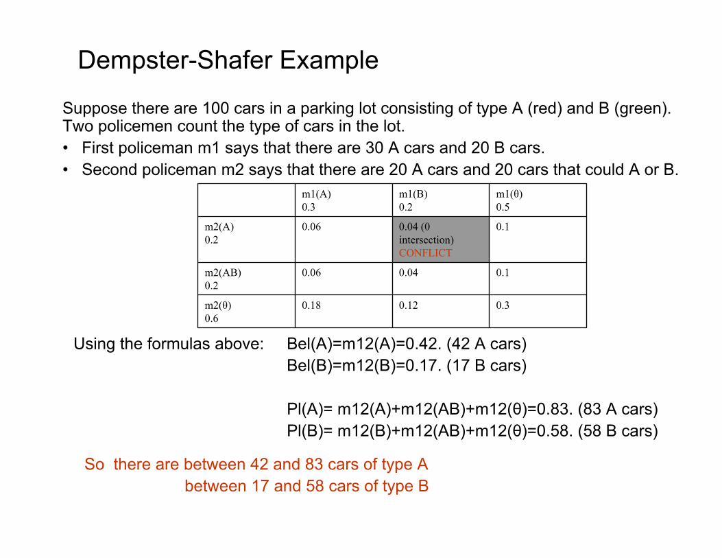
Dempster-Shafer Example

Suppose there are 100 cars in a parking lot consisting of type A (red) and B (green). Two policemen count the type of cars in the lot. • First policeman m1 says that there are 30 A cars and 20 B cars. • Second policeman m2 says that there are 20 A cars and 20 cars that could A or B.

0.30.120.18m2(θ) 0.6

0.10.040.06m2(AB) 0.2

0.10.04 (0 intersection)CONFLICT

0.06m2(A) 0.2

m1(θ)0.5

m1(B)0.2

m1(A)0.3

So there are between 42 and 83 cars of type Abetween 17 and 58 cars of type B

Bel(A)=m12(A)=0.42. (42 A cars)Bel(B)=m12(B)=0.17. (17 B cars)

Pl(A)= m12(A)+m12(AB)+m12(θ)=0.83. (83 A cars)Pl(B)= m12(B)+m12(AB)+m12(θ)=0.58. (58 B cars)

Using the formulas above:

Fuzzy Logic Fault ClassificationUnifies

expert systemsstatisticalneural network approaches

2-D FL system c.f. neural network

Fig 1 FL rulebase to diagnose broken bars in motor drives usingsideband components of vibration signature FFT [Filippetti 2000].

Number of broken bars = none, one, two.Incip. = incipient fault

small medium large

smal

lm

ediu

mla

rge

Sideband component I1

Side

band

com

pone

nt I 2

none incip.

incip.

one

one

one

oneortwo

oneortwo

two

... ..

.........

.................... .

......... . . . ...... .

.. ..

.

. ..

Fig 5 Clustering of statistical fault data

Vibration magnitude

Driv

e tra

in g

ear t

ooth

wea

r

Faul

t con

ditio

ns

one

two

thre

e

low med severe

FL Decision Thresholds

From Chestnut

Based onLegacy fault data historiesManuf. variability dataUsage variabilityMission historyMinimize Pr{false alarm}Baseline perf. requirements

Can be tuned using adaptive learning techniques

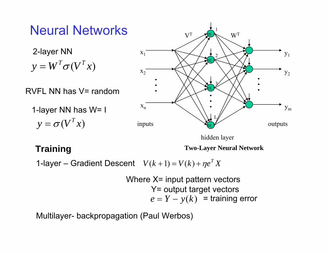
Two-Layer Neural Network

σ(.)

σ(.)

σ(.)

σ(.)

x1

x2

y1

y2

VT WT

inputs

hidden layer

outputs

xn ym

1

2

3

L

Neural Networks

)( xVWy TTσ=

1-layer NN has W= I

)( xVy Tσ=

2-layer NN

RVFL NN has V= random

Training1-layer – Gradient Descent XekVkV Tη+=+ )()1(

Where X= input pattern vectorsY= output target vectors

)(kyYe −= = training error

Multilayer- backpropagation (Paul Werbos)

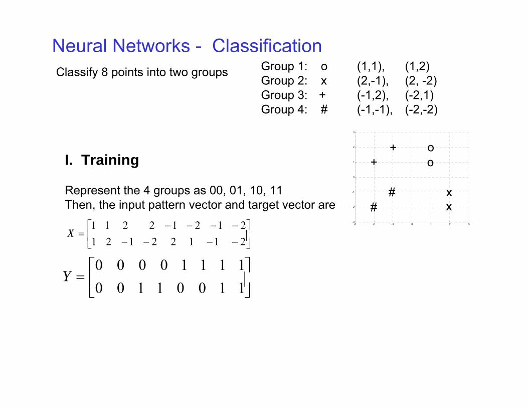
Neural Networks - ClassificationGroup 1: o (1,1), (1,2)Group 2: x (2,-1), (2, -2)Group 3: + (-1,2), (-2,1)Group 4: # (-1,-1), (-2,-2)

Classify 8 points into two groups

-3 -2 -1 0 1 2 3-3

-2

-1

0

1

2

3

oo

xx

++

##

Represent the 4 groups as 00, 01, 10, 11Then, the input pattern vector and target vector are

⎥⎦

⎤⎢⎣

⎡−−−−−−−−

=2112212121212211

X

⎥⎦

⎤⎢⎣

⎡=

1100110011110000

Y

I. Training

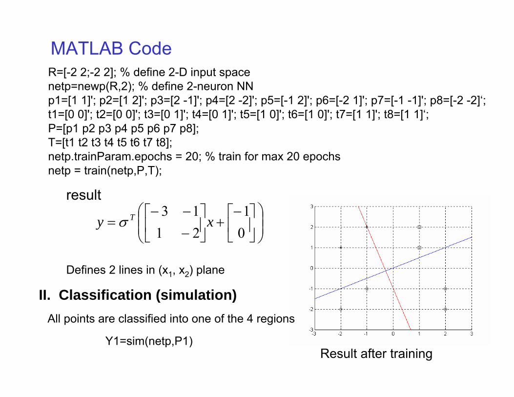
MATLAB CodeR=[-2 2;-2 2]; % define 2-D input spacenetp=newp(R,2); % define 2-neuron NNp1=[1 1]'; p2=[1 2]'; p3=[2 -1]'; p4=[2 -2]'; p5=[-1 2]'; p6=[-2 1]'; p7=[-1 -1]'; p8=[-2 -2]‘;t1=[0 0]'; t2=[0 0]'; t3=[0 1]'; t4=[0 1]'; t5=[1 0]'; t6=[1 0]'; t7=[1 1]'; t8=[1 1]‘;P=[p1 p2 p3 p4 p5 p6 p7 p8];T=[t1 t2 t3 t4 t5 t6 t7 t8];netp.trainParam.epochs = 20; % train for max 20 epochsnetp = train(netp,P,T);

⎟⎟⎠

⎞⎜⎜⎝

⎛⎥⎦

⎤⎢⎣

⎡−+⎥

⎦

⎤⎢⎣

⎡−−−

=01

2113

xy Tσ

result

Result after training

Defines 2 lines in (x1, x2) plane

II. Classification (simulation)All points are classified into one of the 4 regions

Y1=sim(netp,P1)

Clustering Using NNCompetitive NN

Make 2 x 80 matrix P of the 80 points

Given80 datapoints

MATLAB code% make new competitive NN with 8 neurons

net = newc([0 1;0 1],8,.1); % train NN with Kohonen learning

net.trainParam.epochs = 7; net = train(net,P); w = net.IW{1};

%plotplot(P(1,:),P(2,:),'+r');xlabel('p(1)');ylabel('p(2)');hold on;circles = plot(w(:,1),w(:,2),'ob');

I. Training & Clustering

II. Classification (simulation)p = [0; 0.2];a = sim(net,p)

Activates neuron number 1

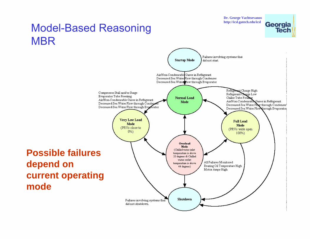
Possible failures depend on current operating mode

Model-Based ReasoningMBR


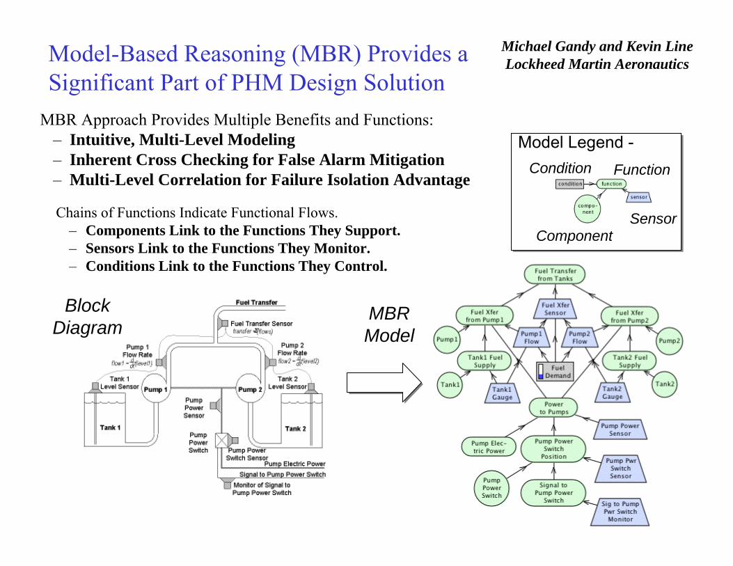
Model Legend -Model Legend -Condition Function

SensorComponent

BlockDiagram

MBRModel

MBR Approach Provides Multiple Benefits and Functions:– Intuitive, Multi-Level Modeling– Inherent Cross Checking for False Alarm Mitigation– Multi-Level Correlation for Failure Isolation Advantage

Chains of Functions Indicate Functional Flows.– Components Link to the Functions They Support.– Sensors Link to the Functions They Monitor.– Conditions Link to the Functions They Control.

Michael Gandy and Kevin LineLockheed Martin AeronauticsModel-Based Reasoning (MBR) Provides a

Significant Part of PHM Design Solution

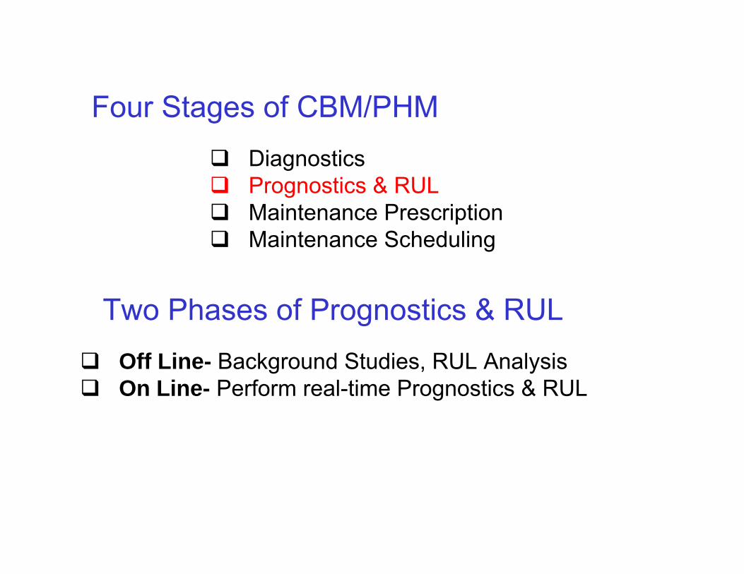
Off Line- Background Studies, RUL AnalysisOn Line- Perform real-time Prognostics & RUL

Two Phases of Prognostics & RUL

Four Stages of CBM/PHMDiagnosticsPrognostics & RULMaintenance PrescriptionMaintenance Scheduling

The CBM/PHM Cycle

MachineSensors

Pre-Processing

FeatureExtraction

FaultClassi-fication

Predictionof Fault

EvolutionData

ScheduleRequired

Maintenance

Systems &Signal processing

Diagnostics PrescriptionMaintenanceScheduling

PrescribeMaintenance

Prognostics

Current fault condition

Required Background Studies

Machine legacy failure data

Available resourcesRULMission due dates

PHMPrognostics

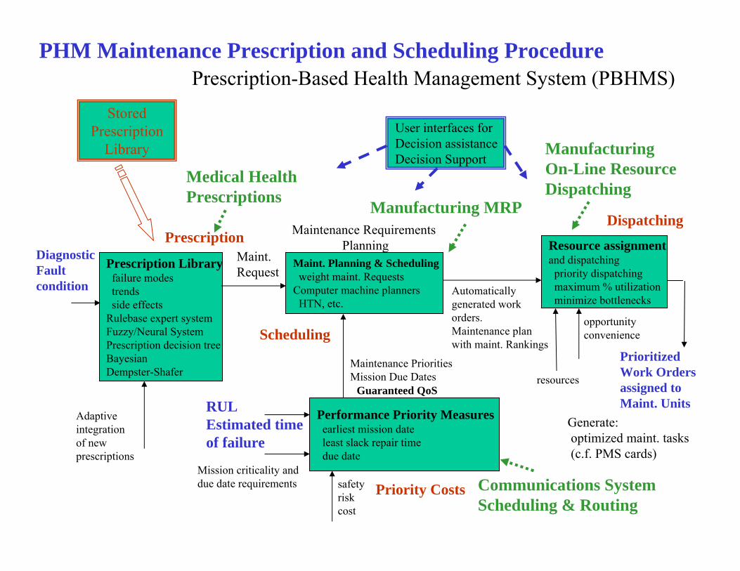
Prescription Libraryfailure modestrendsside effects

Rulebase expert systemFuzzy/Neural SystemPrescription decision treeBayesianDempster-Shafer

DiagnosticFaultcondition

Maint. Request

Maint. Planning & Schedulingweight maint. Requests

Computer machine plannersHTN, etc.

Performance Priority Measuresearliest mission dateleast slack repair timedue date

RULEstimated time of failure

Mission criticality and due date requirements

Maintenance Requirements Planning

Maintenance PrioritiesMission Due Dates

safetyriskcost

opportunityconvenience

Automatically generated work orders.Maintenance plan with maint. Rankings

Resource assignmentand dispatchingpriority dispatchingmaximum % utilizationminimize bottlenecks

resources

PrioritizedWork Ordersassigned toMaint. Units

Guaranteed QoS

User interfaces forDecision assistanceDecision Support

Adaptiveintegrationof newprescriptions

PHM Maintenance Prescription and Scheduling Procedure

StoredPrescription

Library

Medical HealthPrescriptions Manufacturing MRP

Communications SystemScheduling & Routing

ManufacturingOn-Line ResourceDispatching

Prescription-Based Health Management System (PBHMS)

Generate:optimized maint. tasks(c.f. PMS cards)

Prescription

Scheduling

Priority Costs

Dispatching

Fault detection threshold

4%fault

10%fault

failure

ReplaceComponent

Replacesubsystem Replace entire

system

Fault development trend:Progressive escalation of required maintenance

Repair time

Missiondue date

Startrepair

Removefromservice

Estimatedtime of Failure (ETF)

Scheduling Removal From Service and Start of Repair in terms of ETF and Mission Due Date

Prognostics- Why?

I. Fault Propagation & Progression

II. Time of Failure &Remaining Useful Life (RUL)

Impacts the Prescription Impacts the Scheduling

N. Viswanadham

RUL

Presenttime

Progressive Escalation Mission Criticality

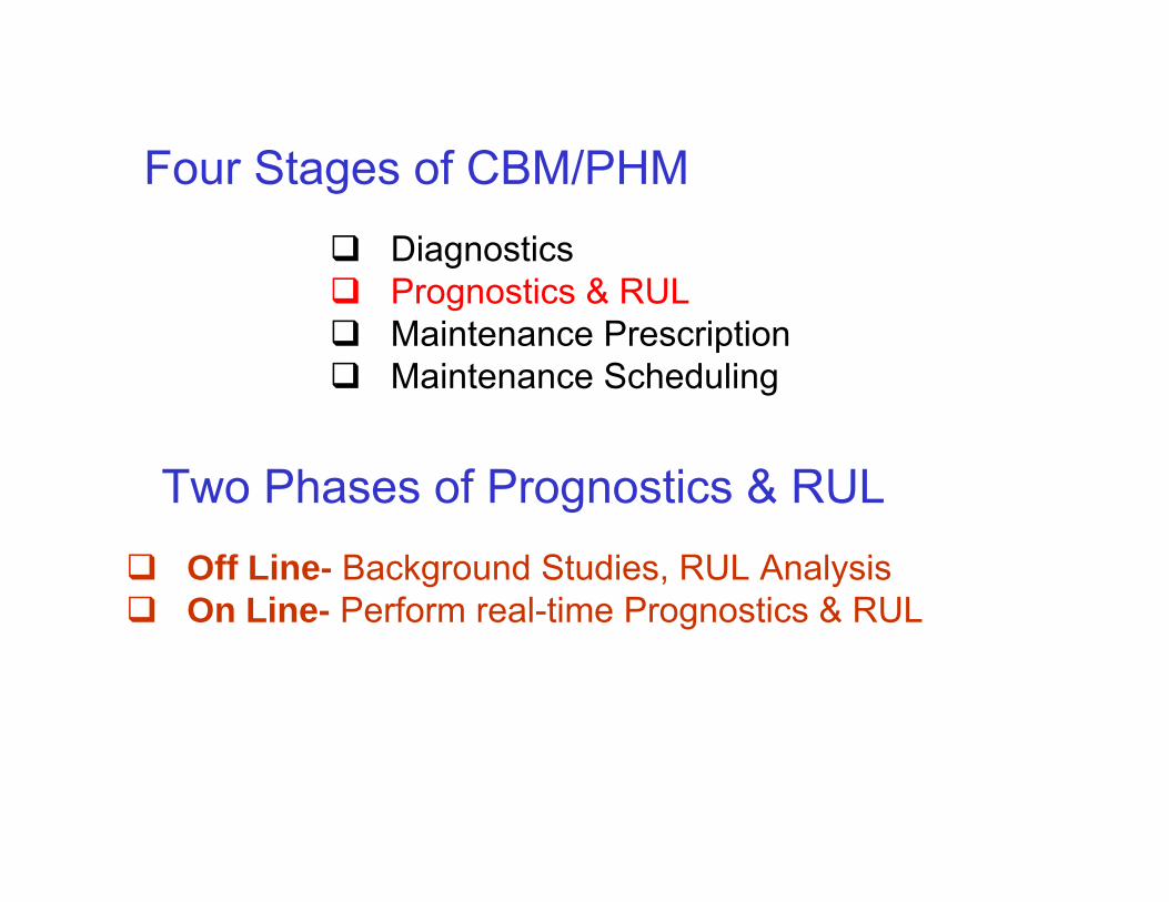
Off Line- Background Studies, RUL AnalysisOn Line- Perform real-time Prognostics & RUL

Two Phases of Prognostics & RUL

Four Stages of CBM/PHMDiagnosticsPrognostics & RULMaintenance PrescriptionMaintenance Scheduling

PHM – Fault Prognostics & RUL Background Studies

• Fault Mode Time Analysis- Identify MTTF in each fault condition

• Identify the best Feature Combinations to track for effective prognosis & RUL

• Identify Best Decision Schemes to compute the feature combinations

• Build Failure Time Pattern Library

Deal with Mean Time to Failure in each Fault condition.ALSO require Confidence Limits

Phase I- Preliminary Off-Line Studies

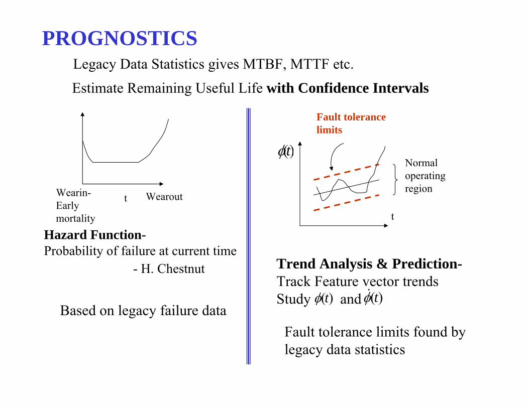
PROGNOSTICS

Hazard Function-Probability of failure at current time

tWearin-Earlymortality

Wearout

Trend Analysis & Prediction-Track Feature vector trendsStudy and)(tφ )(tφ

t

)(tφNormal operatingregion

Fault tolerance limits

Fault tolerance limits found by legacy data statistics

Estimate Remaining Useful Life with Confidence IntervalsLegacy Data Statistics gives MTBF, MTTF etc.

Based on legacy failure data

- H. Chestnut

.

..

. ....

. .....

... ..

....

.............

...... .. . . . ...... .

.. .

.

.

. ..

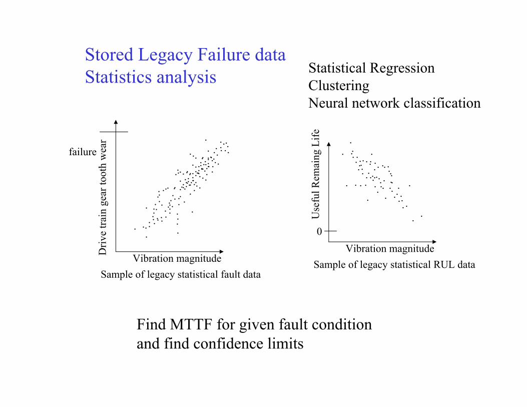
Sample of legacy statistical fault dataVibration magnitudeD

rive

train

gea

r too

th w

ear

failure .

.

. ..

. . ..

.... . . . . . . .. .. .....

.... .

. ..

. . . .. . . . .. .

. . ...... ..

.

.

..

.

Sample of legacy statistical RUL dataVibration magnitude

Use

ful R

emai

ngLi

fe

0

Stored Legacy Failure data Statistics analysis

Find MTTF for given fault conditionand find confidence limits

. . ....

...

. . . ...... ..

. ..

... . .

....

... . . . ...... .

.. .

.

... . ..

....

.. . . ...... .

..

..

Statistical RegressionClusteringNeural network classification

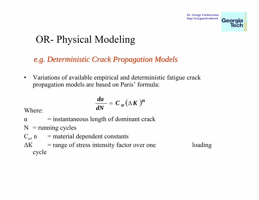
• Variations of available empirical and deterministic fatigue crack propagation models are based on Paris’ formula:

Where:α = instantaneous length of dominant crackΝ = running cyclesCo, n = material dependent constantsΔК = range of stress intensity factor over one loading

cycle

( )no KCdNda

Δ=

e.g. Deterministic Crack Propagation Modelse.g. Deterministic Crack Propagation Models

OR- Physical Modeling


Andy Hess, US Naval Air

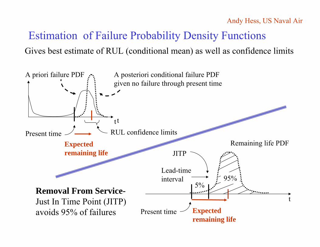
Estimation of Failure Probability Density FunctionsGives best estimate of RUL (conditional mean) as well as confidence limits

A priori failure PDF A posteriori conditional failure PDFgiven no failure through present time

Present timeExpected remaining life

RUL confidence limitst

Remaining life PDF

Expected remaining life

Present time

5%95%

t

t

Lead-timeinterval

JITP

Removal From Service-Just In Time Point (JITP) avoids 95% of failures

Andy Hess, US Naval Air

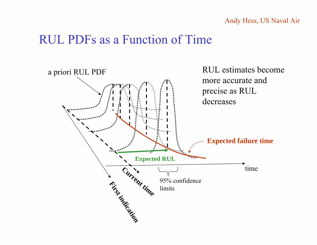
RUL PDFs as a Function of Time

Current time

First indication

timeExpected RUL

RUL estimates become more accurate and precise as RUL decreases

a priori RUL PDF

Expected failure time

95% confidencelimits

Kalman Filter is the optimal estimator for the conditional PDF for linear Gaussian case-gives estimate plus

covariance

t

)(tφNormal operatingregion

Fault tolerance limits

Confidence limits

Estimated feature

alarm

failure

Minimize Pr{false alarm}Pr{miss}

Model-Based Predictive Methods- Mike Grimble

Fault Trend Analysis

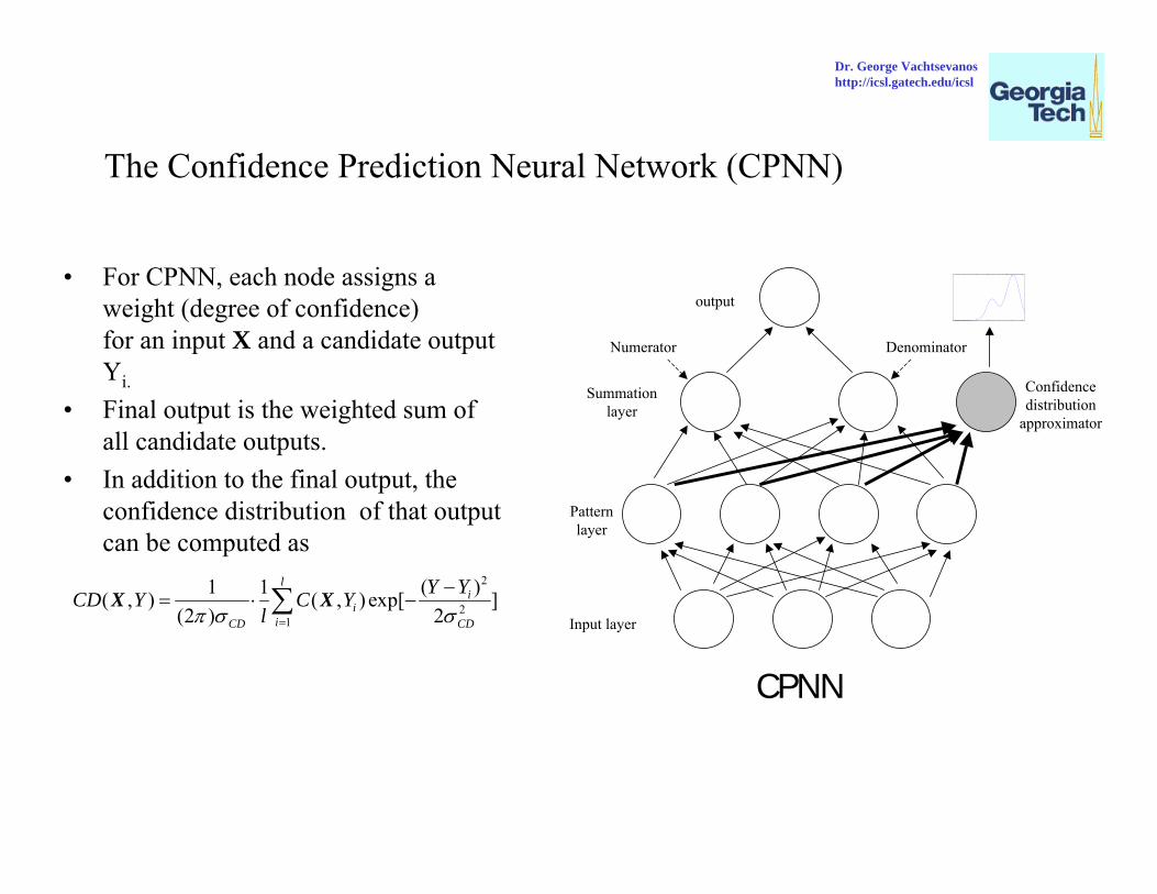
The Confidence Prediction Neural Network (CPNN)

• For CPNN, each node assigns a weight (degree of confidence) for an input X and a candidate output Yi.

• Final output is the weighted sum of all candidate outputs.

• In addition to the final output, the confidence distribution of that output can be computed as

2

21

( )1 1( , ) ( , ) exp[ ](2 ) 2

li

iiCD CD

Y YCD Y C Ylπ σ σ=

−= ⋅ −∑X X

Input layer

Patternlayer

Summationlayer

output

Numerator Denominator

Confidencedistribution

approximator

CPNN


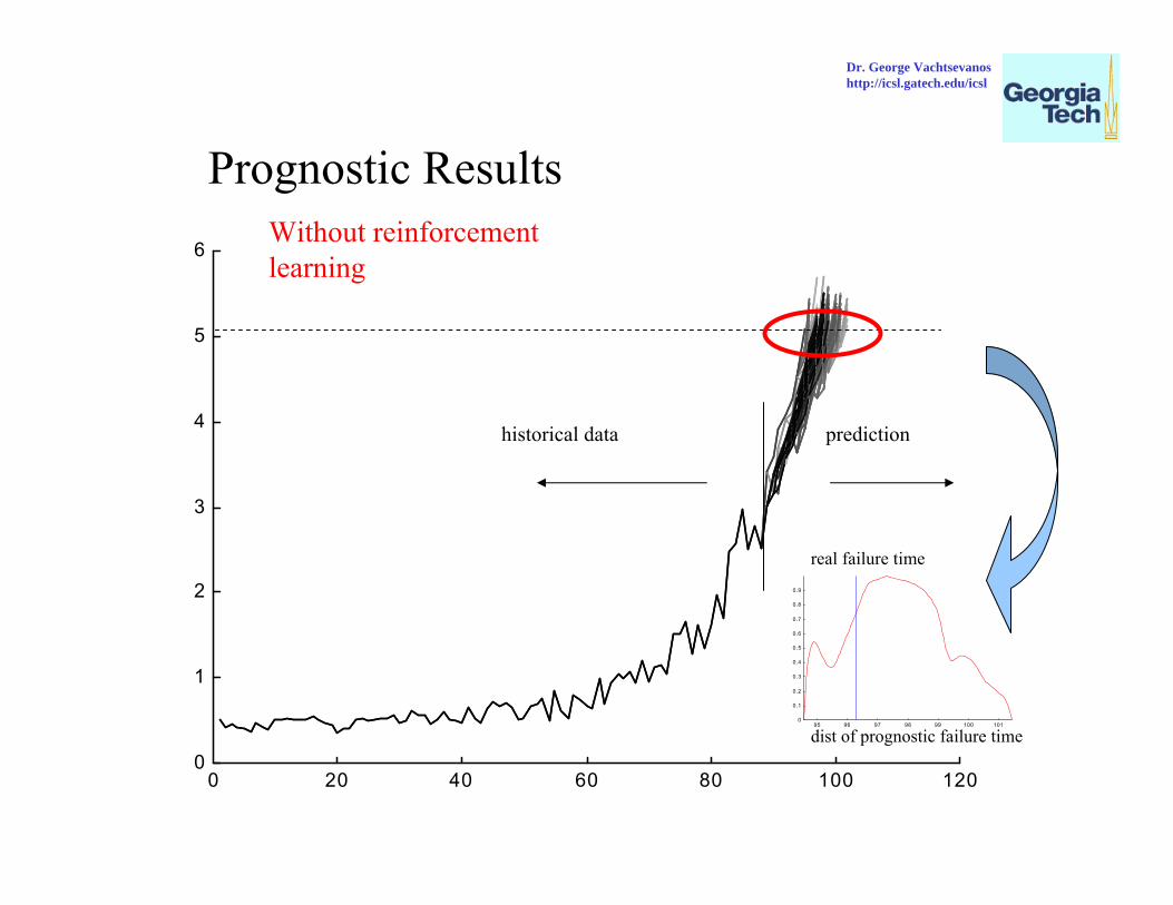
0 20 40 60 80 100 1200

1

2

3

4

5

6

Prognostic ResultsWithout reinforcement learning

historical data prediction

95 96 97 98 99 100 1010

0.1

0.2

0.3

0.4

0.5

0.6

0.7

0.8

0.9

real failure time

dist of prognostic failure time


0 20 40 60 80 100 1200

1

2

3

4

5

6

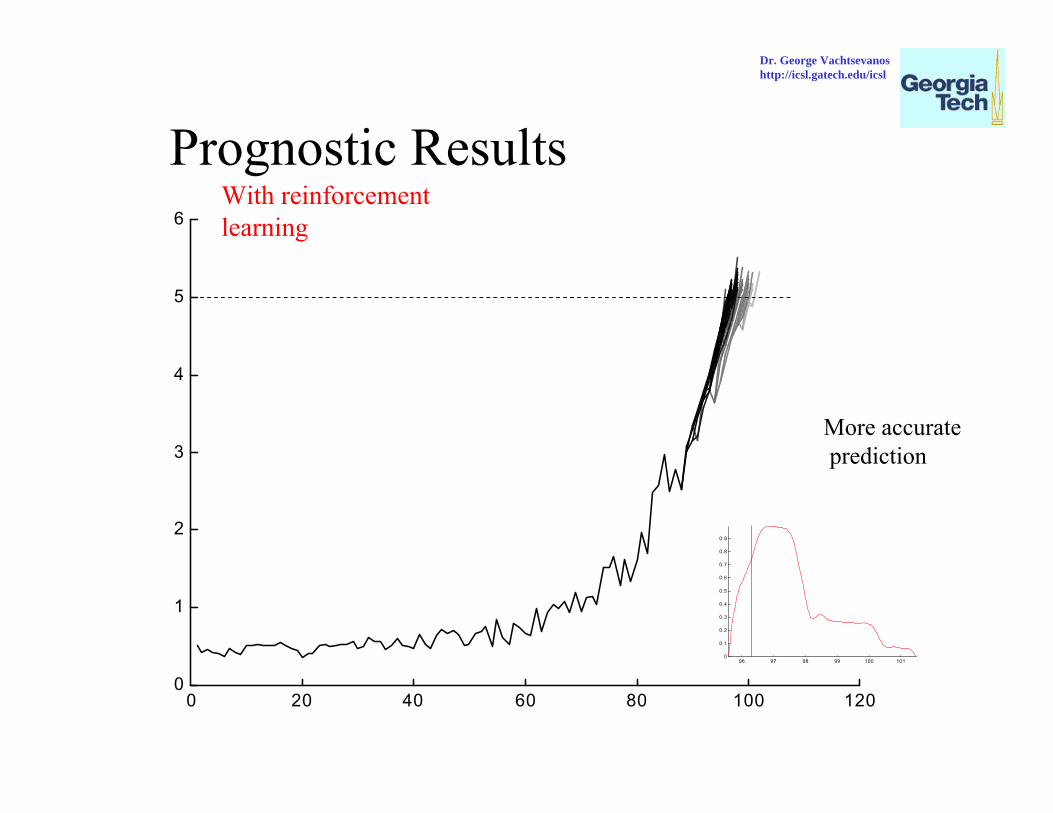
Prognostic ResultsWith reinforcement learning

96 97 98 99 100 1010

0.1

0.2

0.3

0.4

0.5

0.6

0.7

0.8

0.9

More accurateprediction


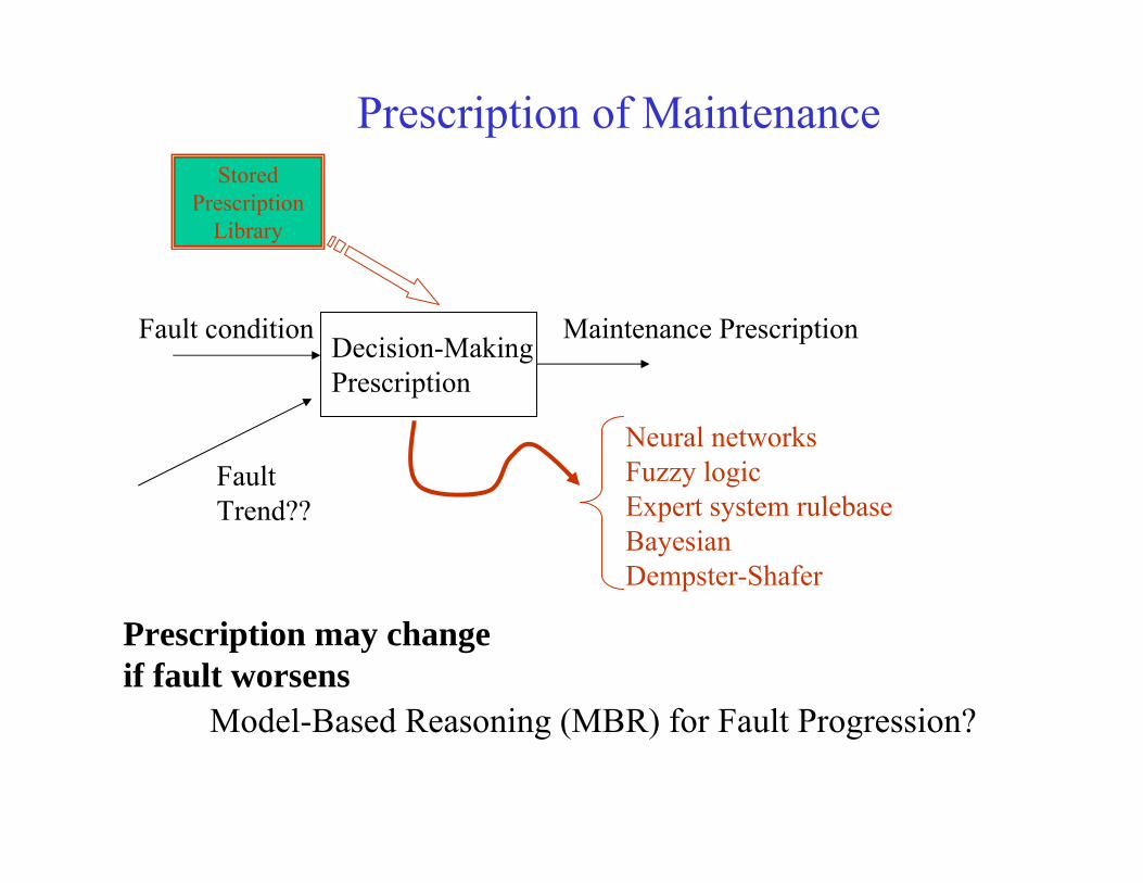
Prescription of Maintenance

Decision-MakingPrescription

StoredPrescription

Library

Fault condition Maintenance Prescription

Neural networksFuzzy logicExpert system rulebaseBayesianDempster-Shafer

Model-Based Reasoning (MBR) for Fault Progression?

Prescription may change if fault worsens

FaultTrend??

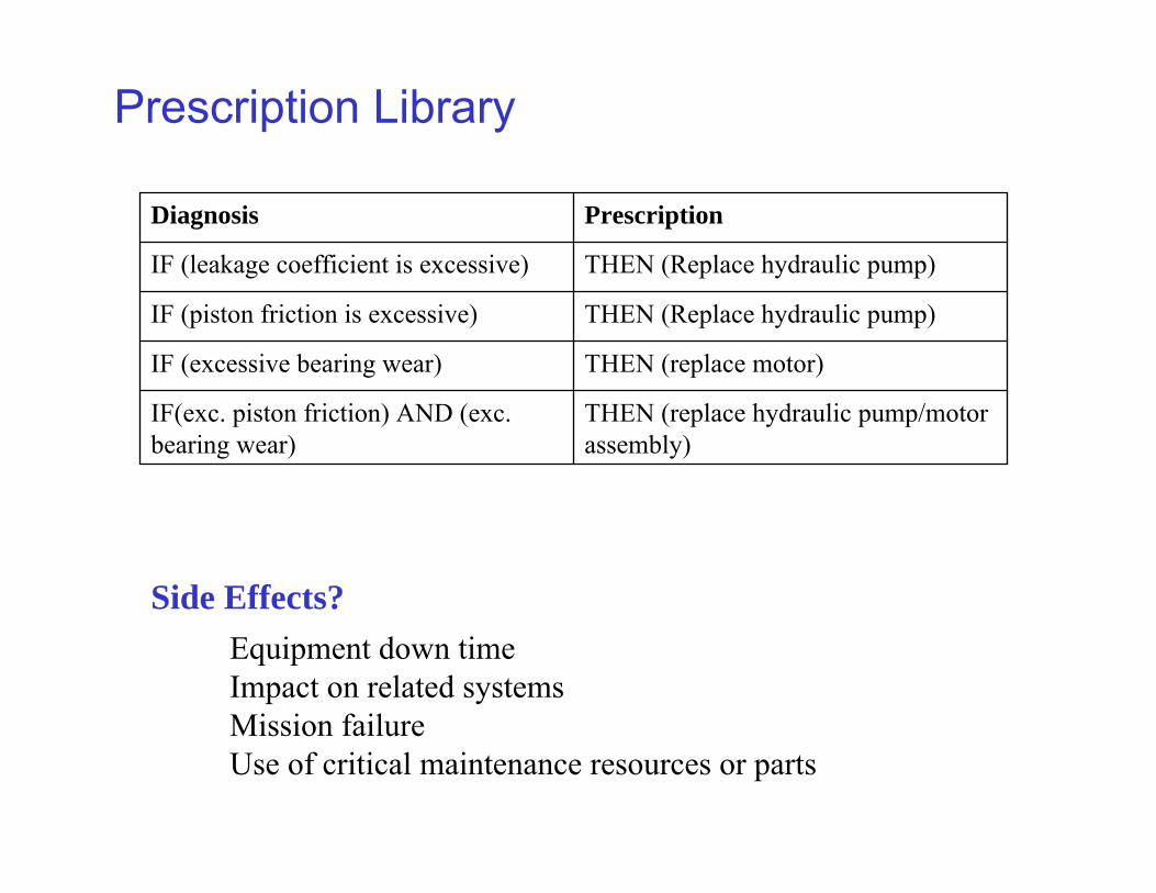
THEN (replace hydraulic pump/motor assembly)

IF(exc. piston friction) AND (exc. bearing wear)

THEN (replace motor)IF (excessive bearing wear)

THEN (Replace hydraulic pump)IF (piston friction is excessive)

THEN (Replace hydraulic pump)IF (leakage coefficient is excessive)

PrescriptionDiagnosis

Prescription Library

Side Effects?Equipment down timeImpact on related systemsMission failureUse of critical maintenance resources or parts

A Maintenance Management Architecture

Enabling TechnologiesGenetic Algorithms for Optimum Maintenance SchedulingCase-Based Reasoning and InductionCost-Benefit Analysis Studies

Real-time Diagnostics /Prognostics

and Trend Analysis

Real-time Diagnostics /Prognostics

and Trend Analysis

OtherProcess

ManagementComponent

(ERP)

OtherProcess

ManagementComponent

(ERP)• Actions Taken• Conditions Found• Cost Collector

• Actions Taken• Conditions Found• Cost Collector

• Material Required • Labor Required• Work Procedures

• Material Required • Labor Required• Work Procedures

Work OrderBacklog

Work OrderBacklog

• Trend Data• Logs• Trend Data• Logs

• Technical Doc Ref• Preplanned Work• Technical Doc Ref• Preplanned Work

• Emergent Work• Emergent Work

Case LibraryCase Library

Time-Directed Tasks

Corrective Tasks

Maintenance Schedule


Time domain - Moments, statistics, correlation, moving averagesFrequency Domain - Discrete Fourier TransformDynamical System Theory

State Estimation- Kalman Filter System Identification- Recursive Least Squares (RLS)

Statistical TechniquesRegressionPDF estimation

Decision-Making TechniquesBayesianDempster-ShaferRule-Based & Expert SystemsFuzzy Logic

Neural NetworksClassificationClustering

Signal Processing and Decision-Making

Aircraft Nose Wheel Shimmy• Nose wheel can vibrate during landing• Divergent vibration is more likely when nose gear free play is

high and tire is worn• Two approaches

– Monitor and trend free play before taxi – Monitor and trend vibration on landing

Good Nose Gear

Landing Gear with Possible Divergent Shimmy

Shimmy Vibration Measurement

Force

Measured Free Play

θ


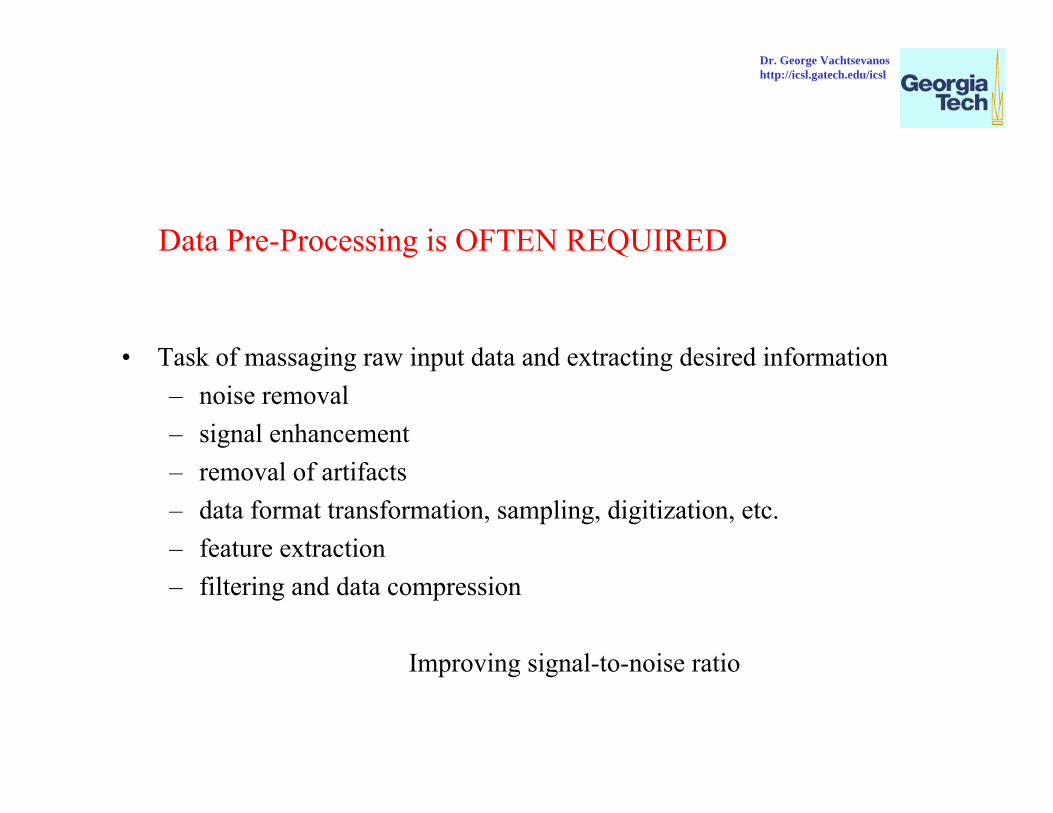
Data Pre-Processing is OFTEN REQUIRED

• Task of massaging raw input data and extracting desired information– noise removal– signal enhancement– removal of artifacts– data format transformation, sampling, digitization, etc.– feature extraction– filtering and data compression

Improving signal-to-noise ratio


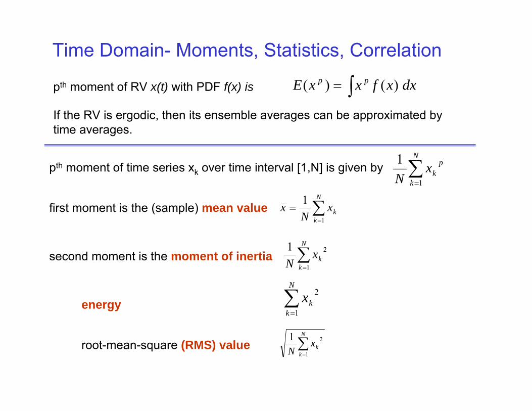
Time Domain- Moments, Statistics, Correlation

∫= dxxfxxE pp )()(pth moment of RV x(t) with PDF f(x) is

If the RV is ergodic, then its ensemble averages can be approximated by time averages.

∑=

N

k

pkx

N 1

1pth moment of time series xk over time interval [1,N] is given by

first moment is the (sample) mean value ∑=

=N

kkx

Nx

1

1

second moment is the moment of inertia ∑=

N

kkx

N 1

21

∑=

N

kkx

1

2

energy

root-mean-square (RMS) value ∑=

N

kkx

N 1

21

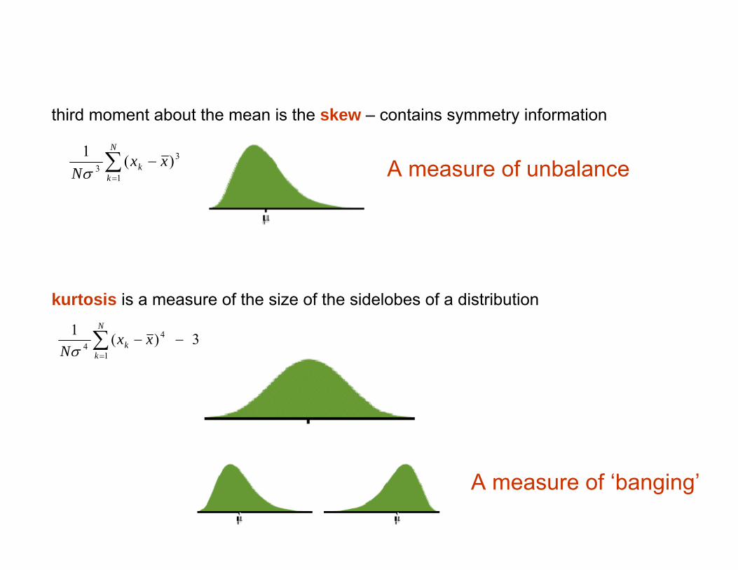
third moment about the mean is the skew – contains symmetry information

∑=

−N

kk xx

N 1

33 )(1

σ

kurtosis is a measure of the size of the sidelobes of a distribution

3)(11

44 −−∑

=

N

kk xx

Nσ

A measure of unbalance

A measure of ‘banging’

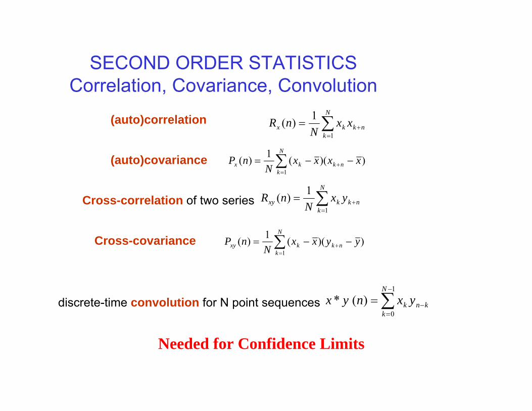
SECOND ORDER STATISTICSCorrelation, Covariance, Convolution

∑=

+=N

knkkx xx

NnR

1

1)((auto)correlation

∑=

+ −−=N

knkkx xxxx

NnP

1

))((1)((auto)covariance

∑=

+=N

knkkxy yx

NnR

1

1)(Cross-correlation of two series

∑=

+ −−=N

knkkxy yyxx

NnP

1))((1)(Cross-covariance

∑−

=−=

1

0)(*

N

kknk yxnyxdiscrete-time convolution for N point sequences

Needed for Confidence Limits

Statistical Tools for Estimating the PDF

.

..

. ....

. .....

... ..

....

.............

...... .. . . . ...... .

.. .

.

.

. ..

Sample of legacy statistical fault dataVibration magnitudeD

rive

train

gea

r too

th w

ear

failure

. . ....

...

. . . ...... ..

. ..

... . .

....

... . . . ...... .

.. .

.

... . ..

....

.. . . ...... .

..

..

Consistent estimator for the joint PDF is

⎥⎦

⎤⎢⎣

⎡ −−⎥

⎦

⎤⎢⎣

⎡ −−−= ∑

=++ 2

2

1212/)1( 2

)(exp2

)()(exp1)2(

1),(σσσπ

iN

i

iTi

nn

zzxxxxN

zxP

∫∫=

dzzxp

dzzxzpxzE

),(

),(]/[

Conditional expected value formula

yields estimate for x given z

∑

∑

=

=

⎥⎦

⎤⎢⎣

⎡ −−−

⎥⎦

⎤⎢⎣

⎡ −−−

=N

i

iTi

N

i

iTii

xxxx

xxxxzxzE

12

12

2)()(exp

2)()(exp

]/[

σ

σ

Given statistical data

This also gives error covariance or Confidence measure

(xi,yi)

Parzen estimator for PDF

= sum of Gaussians

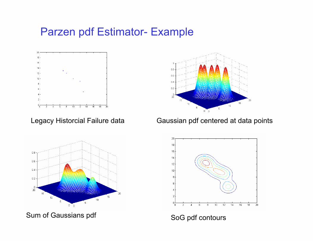
Parzen pdf Estimator- Example

Legacy Historcial Failure data Gaussian pdf centered at data points

Sum of Gaussians pdf SoG pdf contours

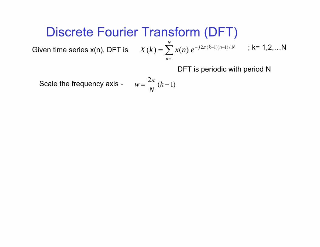
Discrete Fourier Transform (DFT)∑=

−−−=N

n

NnkjenxkX1

/)1)(1(2)()( πGiven time series x(n), DFT is ; k= 1,2,…N

DFT is periodic with period N

)1(2−= k

Nw πScale the frequency axis -

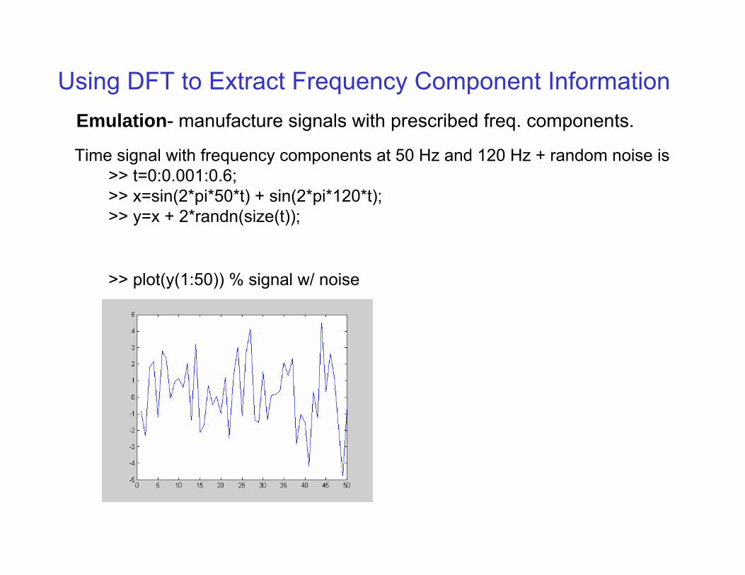
Using DFT to Extract Frequency Component Information

Time signal with frequency components at 50 Hz and 120 Hz + random noise is >> t=0:0.001:0.6;>> x=sin(2*pi*50*t) + sin(2*pi*120*t);>> y=x + 2*randn(size(t));

Emulation- manufacture signals with prescribed freq. components.

>> plot(y(1:50)) % signal w/ noise

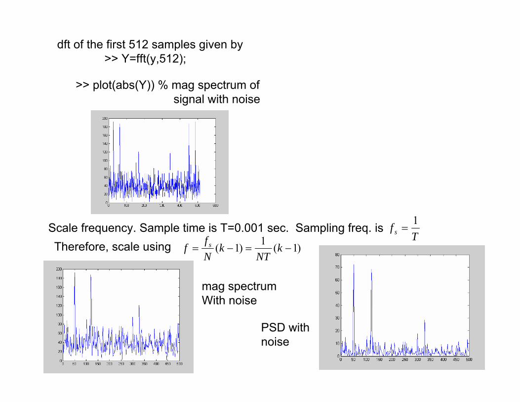
dft of the first 512 samples given by>> Y=fft(y,512);

>> plot(abs(Y)) % mag spectrum of signal with noise

Scale frequency. Sample time is T=0.001 sec. Sampling freq. isT

f s1

=

Therefore, scale using )1(1)1( −=−= kNT

kNf

f s

mag spectrumWith noise

PSD withnoise

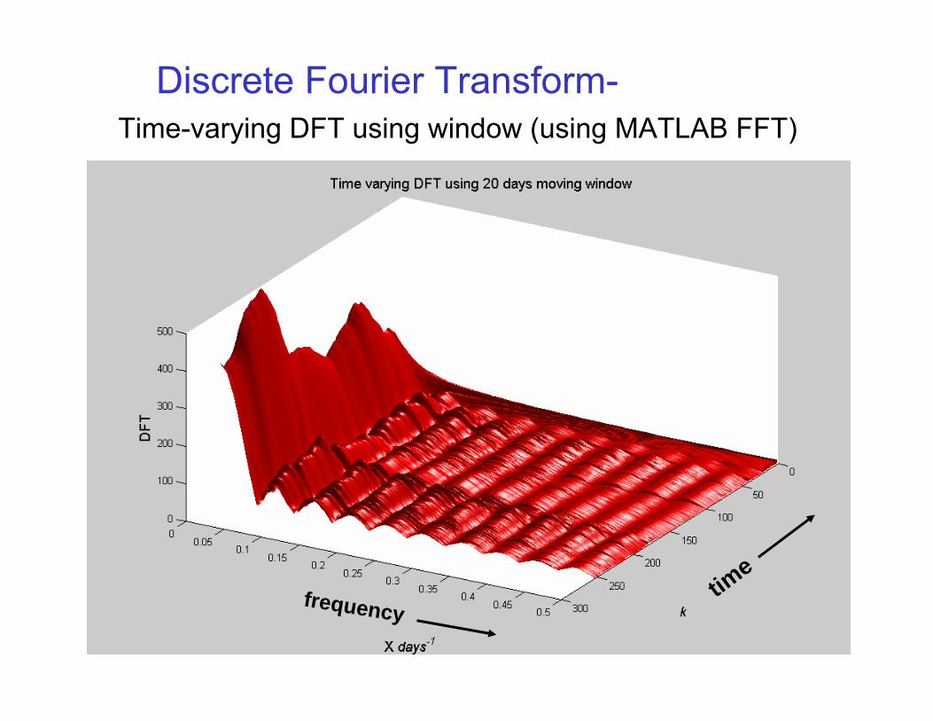
Time-varying DFT using window (using MATLAB FFT)

time

frequency

Discrete Fourier Transform-

1

2

3

4

5

6

7

8

050

100150

200250

300350

400450

500

0

500

1000

(sec)

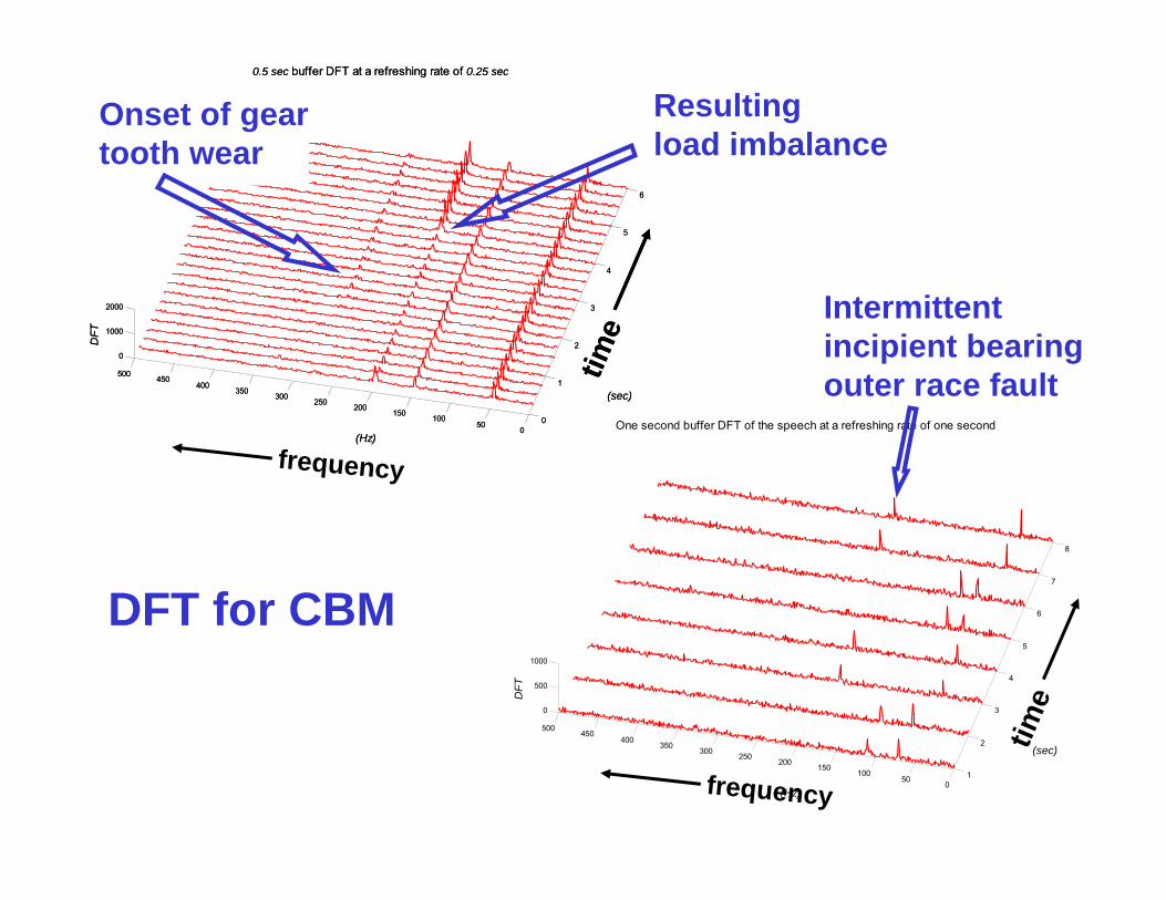
One second buffer DFT of the speech at a refreshing rate of one second

(Hz)

DFT

0

1

2

3

4

5

6

050

100150

200250

300350

400450

500

0

1000

2000

(sec)

0.5 sec buffer DFT at a refreshing rate of 0.25 sec

(Hz)

DFT

time

0

1

2

3

4

5

6

050

100150

200250

300350

400450

500

0

1000

2000

(sec)

0.5 sec buffer DFT at a refreshing rate of 0.25 sec

(Hz)

DFT

time

time

frequency

Intermittentincipient bearingouter race fault

Onset of geartooth wear

Resulting load imbalance

frequency

DFT for CBM

Planetary Gear Transmission

McFadden’s Method


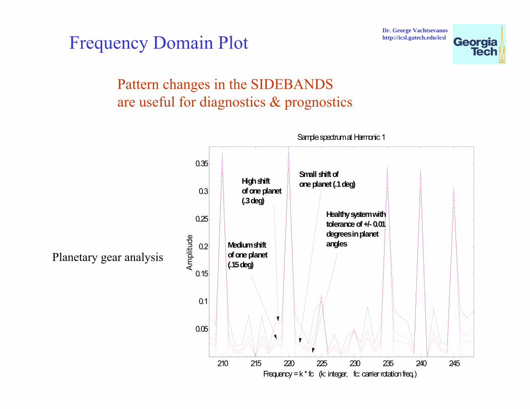
Effect of angular shift of the planets on the model spectrum

• “Ideal” system presents sidebands only at frequencies that are integer multiples of the number of planets

• By “Ideal” meaning that the planets are evenly spaced with zero tolerance

210 215 220 225 230 235 240 2450

0.2

0.4

0.6

0.8

1

1.2

Frequency = k * fc (k:integer, fc: carrier rotation freq.)

Am

plitu

de

Sample spectrum of ideal system

First Harmonicof the Meshing FrequencyZero and non-zero phenomenonis true for any harmonicFourier Coefficients

at frequencies that areinteger multiples of thenumber of planetsare non-zero

All other coefficientsare zero


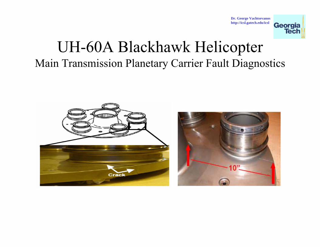
UH-60A Blackhawk HelicopterMain Transmission Planetary Carrier Fault Diagnostics


210 215 220 225 230 235 240 245

0.05

0.1

0.15

0.2

0.25

0.3

0.35

Frequency = k * fc (k: integer, fc: carrier rotation freq.)

Am

plitu

de

Sample spectrum at Harmonic 1

Small shift ofone planet (.1 deg)

Healthy system withtolerance of +/- 0.01degrees in planet anglesMedium shift

of one planet(.15 deg)

High shiftof one planet(.3 deg)

Frequency Domain Plot Dr. George Vachtsevanoshttp://icsl.gatech.edu/icsl

Pattern changes in the SIDEBANDS are useful for diagnostics & prognostics

Planetary gear analysis

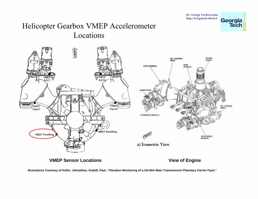
VMEP Sensor Locations View of Engine

Illustrations Courtesy of Keller, Johnathan, Grabill, Paul, “Vibration Monitoring of a UH-60A Main Transmission Planetary Carrier Fault.”

Helicopter Gearbox VMEP Accelerometer Locations


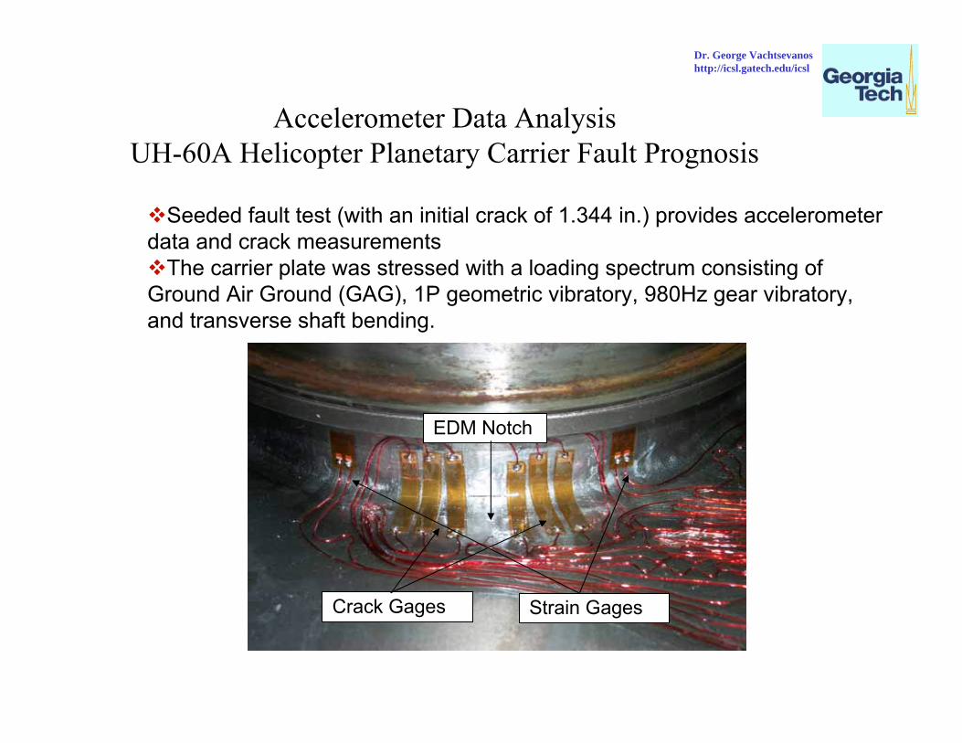
Accelerometer Data Analysis UH-60A Helicopter Planetary Carrier Fault Prognosis

Seeded fault test (with an initial crack of 1.344 in.) provides accelerometer data and crack measurements

The carrier plate was stressed with a loading spectrum consisting of Ground Air Ground (GAG), 1P geometric vibratory, 980Hz gear vibratory, and transverse shaft bending.

EDM Notch

Crack Gages Strain Gages


0 200 400 600 800 1000 1200 1400 1600 1800 2000

0

0.5

1

1.5

2

2.5

3

3.5

4

4.5

TSA data in the frequency domain

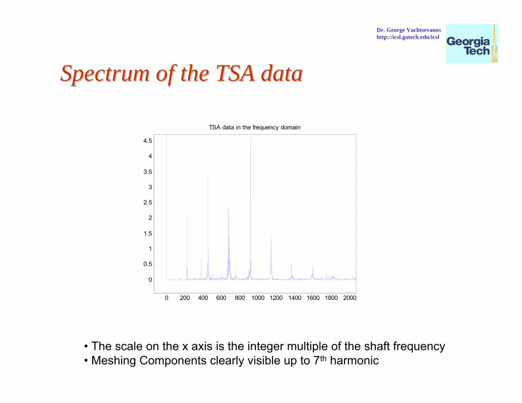
Spectrum of the TSA dataSpectrum of the TSA data

• The scale on the x axis is the integer multiple of the shaft frequency• Meshing Components clearly visible up to 7th harmonic


Spectrum Changes as Test ProgressesSpectrum Changes as Test Progresses

215 220 225 230 235 240

0

0.5

1

1.5

2

2.5Dominant Frequency

Apparent Frequency

215 220 225 230 235 240

0

0.5

1

1.5

2

2.5Dominant Frequency

Apparent Frequency

Green for data at GAG #9Blue for GAG #260Red for GAG #639

The decrease of the dominant frequency as well as the other apparent frequencies and the increase of the rest may be a good sign of the crack growth, and may be quantified as features for fault diagnosis and prognosis purposes.

Spectrum content around the fundamental meshing frequency


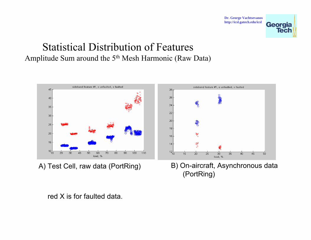
Statistical Distribution of FeaturesAmplitude Sum around the 5th Mesh Harmonic (Raw Data)

red X is for faulted data.

A) Test Cell, raw data (PortRing) B) On-aircraft, Asynchronous data (PortRing)


( )

( )

( )

1

1

11

ˆ ˆ ˆ ,

,

.

k k k k k k

T Tk k k

T T T Tk k k k k

x Ax Bu AK z Hx

K P H HP H R

P A P P H HP H R HP A GQG

− − −+

−− −

−− − − − −+

= + + −

= +

⎡ ⎤= − + +⎢ ⎥⎣ ⎦

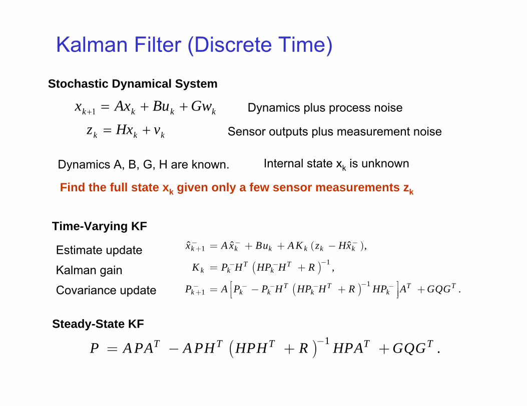
Kalman Filter (Discrete Time)

Estimate update

Kalman gain

Covariance update

( ) 1.T T T T TP APA APH HPH R HPA GQG

−= − + +

Steady-State KF

Time-Varying KF

kkkk GwBuAxx ++=+1

kkk vHxz +=

Stochastic Dynamical System

Dynamics plus process noise

Sensor outputs plus measurement noise

Dynamics A, B, G, H are known. Internal state xk is unknown

Find the full state xk given only a few sensor measurements zk

KF Also Gives Error Covariance- a measure of accuracy and

confidence in the estimate

0 1 2 3

errorcovariancea priorierror covariance

a posteriorierror covariance P0 P1 P2 P3

time

time u

pdate

(TU)

TU MUMU TU

MU

mea

s. up

date

P1 P2 P3

Error covariance update timing diagram

Automation & Robotics Research Institute (ARRI)The University of Texas at Arlington

F.L. LewisMoncrief-O’Donnell Endowed Chair

Head, Controls & Sensors Group

http://ARRI.uta.edu/[email protected]

CBM- ARRI Testbed

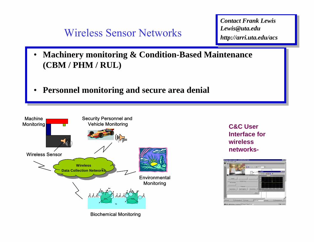
Wireless Sensor Networks

• Machinery monitoring & Condition-Based Maintenance (CBM / PHM / RUL)

• Personnel monitoring and secure area denial

Contact Frank [email protected]://arri.uta.edu/acs

Contact Frank [email protected]://arri.uta.edu/acs

C&C UserInterface forwireless networks-

WirelessData Collection Networks

Wireless Sensor

Machine Monitoring

Security Personnel and Vehicle Monitoring

C

O O

HH2O

h+

h+

h+

H2OC

O O

H

C

O O

H

C

O O

HC

O O

H h+

C

O O

H

C

O O

H

C

O O

H

C

O O

H

C

O O

H

C

O O

H

e-

e-

e-

e-

TiO2TiO2

Ni

C

O O

H

C

O O

HH2O

h+

h+h+

h+

H2OC

O O

H

C

O O

H

C

O O

H

C

O O

H

C

O O

H

C

O O

H

C

O O

HC

O O

H

CO O

H h+

C

O O

H

C

O O

H

C

O O

H

C

O O

H

C

O O

H

C

O O

H

C

O O

H

C

O O

H

C

O O

H

C

O O

H

C

O O

H

C

O O

H

e-

e-

e-

e-

TiO2TiO2

Ni

Biochemical Monitoring

EnvironmentalMonitoring

WirelessData Collection Networks

Wireless Sensor

Machine Monitoring

Security Personnel and Vehicle Monitoring

C

O O

HH2O

h+

h+

h+

H2OC

O O

H

C

O O

H

C

O O

HC

O O

H h+

C

O O

H

C

O O

H

C

O O

H

C

O O

H

C

O O

H

C

O O

H

e-

e-

e-

e-

TiO2TiO2

Ni

C

O O

H

C

O O

HH2O

h+

h+h+

h+

H2OC

O O

H

C

O O

H

C

O O

H

C

O O

H

C

O O

H

C

O O

H

C

O O

HC

O O

H

CO O

H h+

C

O O

H

C

O O

H

C

O O

H

C

O O

H

C

O O

H

C

O O

H

C

O O

H

C

O O

H

C

O O

H

C

O O

H

C

O O

H

C

O O

H

e-

e-

e-

e-

TiO2TiO2

Ni

Biochemical Monitoring

EnvironmentalMonitoring

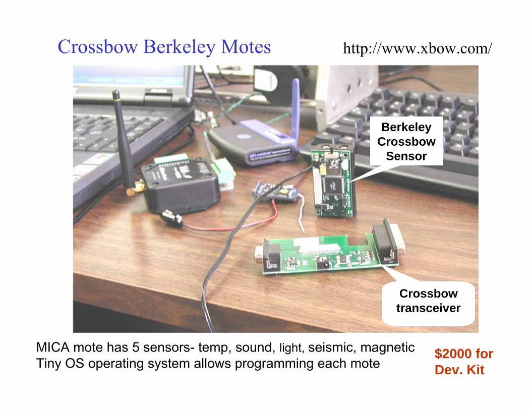
Berkeley Crossbow

Sensor

Crossbow transceiver

Crossbow Berkeley Motes http://www.xbow.com/

MICA mote has 5 sensors- temp, sound, light, seismic, magneticTiny OS operating system allows programming each mote

$2000 forDev. Kit

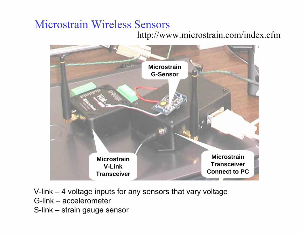
MicrostrainV-Link

Transceiver

MicrostrainTransceiver

Connect to PC

MicrostrainG-Sensor

Microstrain Wireless Sensorshttp://www.microstrain.com/index.cfm

V-link – 4 voltage inputs for any sensors that vary voltageG-link – accelerometerS-link – strain gauge sensor

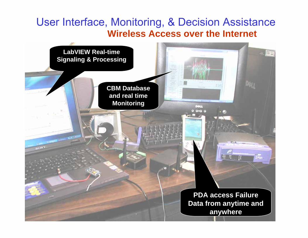
LabVIEW Real-time Signaling & Processing

CBM Database and real time Monitoring

PDA access Failure Data from anytime and

anywhere

User Interface, Monitoring, & Decision AssistanceWireless Access over the Internet

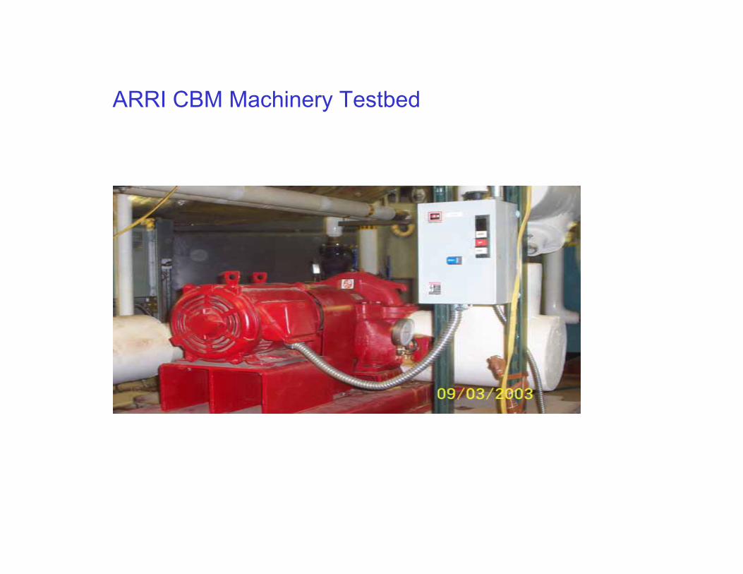
ARRI CBM Machinery Testbed

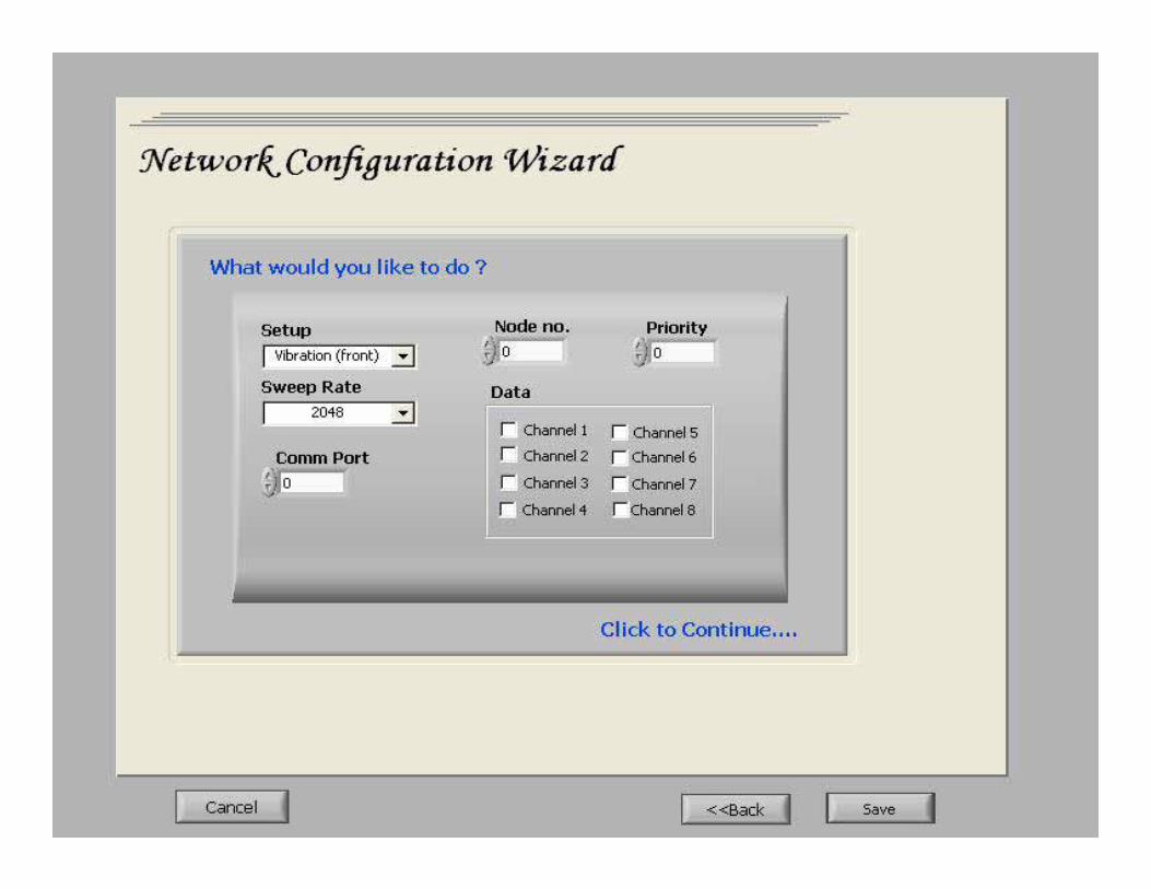
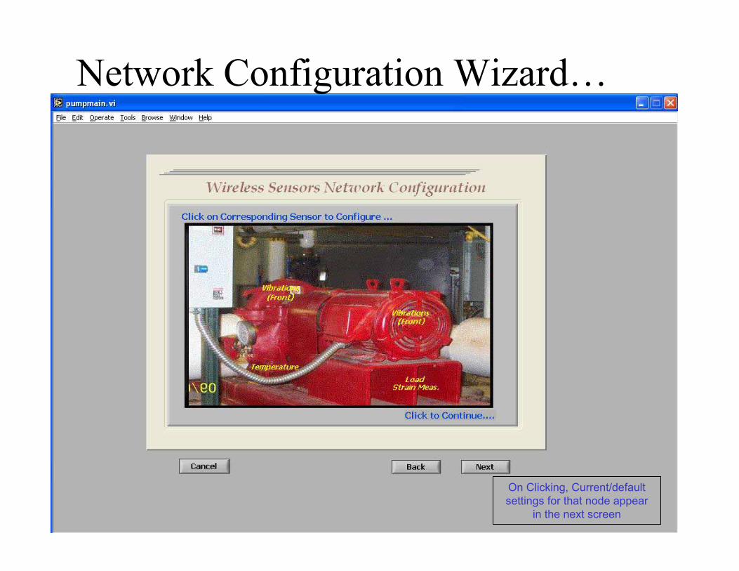
Network Configuration Wizard…

On Clicking, Current/default settings for that node appear

in the next screen

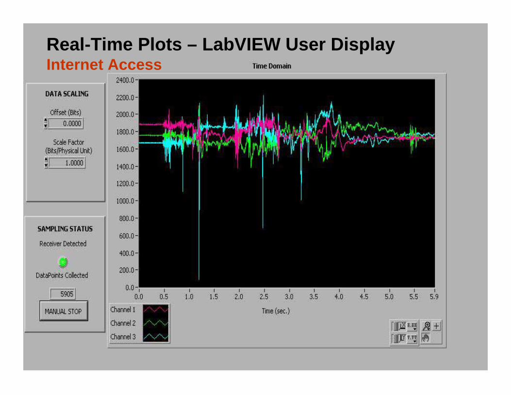
Real-Time Plots – LabVIEW User DisplayInternet Access

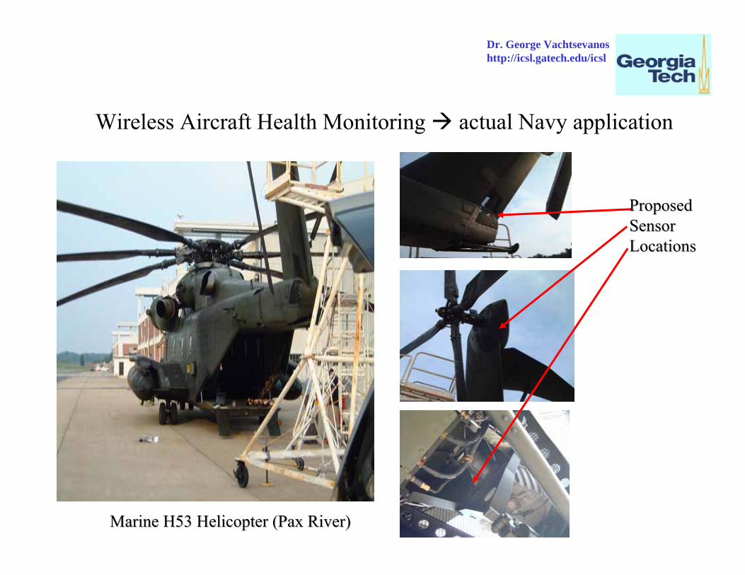
Wireless Aircraft Health Monitoring actual Navy application

ProposedProposedSensor Sensor LocationsLocations

Marine H53 Helicopter (Marine H53 Helicopter (PaxPax River)River)


Documents

Intelligent Fault Diagnosis & Prognosis - UTA talks/Metrocon 07 intel diag and prog... · New Business Models for ... Periodic, whether needed or not Run-to-Failure No maintenance