TOPICAL REPORT

Intelligent Computing System for Reservoir Analysisand Risk Assessment of the Red River Formation

ByMark A. Sippel

October 2001

Work Performed under Contract No. DE-FC26-00BC15123

Prepared for:

U.S. Department of EnergyAssistant Secretary for Fossil Energy

Daniel FergusonNational Petroleum Technology Office

P.O. Box 3628Tulsa, OK 74101

Prepared by:Luff Exploration Company

1580 Lincoln Street, Suite 850Denver, CO 80203

i

Intelligent Computing System for Reservoir Analysisand Risk Assessment of the Red River Formation

COOPERATIVE AGREEMENT DE- FC26-00BC15123

Disclaimer

This report was prepared as an account of work sponsored by an agency of the UnitedStates Government. Neither the United States Government nor any agency thereof, northeir employees, makes any warranty, expressed or implied, or assumes any legal liabilityor responsibility for the accuracy, completeness, or usefulness of any information,apparatus, product, or process disclosed or represented that its use would not infringeprivately owned rights. Reference herein to any specific commercial product, process, orservice by trade name, trademark, manufacturer, or otherwise does not necessarilyconstitute or imply its endorsement, recommendation, or favoring by the United StatesGovernment or any agency thereof. The views and opinions of authors expressed hereindo not necessarily state or reflect those of the United States Government or any agencythereof.

ii

ABSTRACT

Integrated software has been written that comprises the tool kit for the IntelligentComputing System (ICS). The software tools in ICS are for evaluating reservoir andhydrocarbon potential from various seismic, geologic and engineering data sets. The ICStools provide a means for logical and consistent reservoir characterization. The tools canbe broadly characterized as 1) clustering tools, 2) neural solvers, 3) multiple-linearregression, 4) entrapment-potential calculator and 5) combining tools. A flexibleapproach can be used with the ICS tools. They can be used separately or in a series tomake predictions about a desired reservoir objective. The tools in ICS are primarilydesigned to correlate relationships between seismic information and data obtained fromwells; however, it is possible to work with well data alone.

iii

EXECUTIVE SUMMARY

This report contains descriptions of software tools for aiding companies and individualsin their efforts to extract the most information from geophysical, geological andengineering data in the pursuit of oil exploration and development. The primary objectiveof this project is to construct software tools for an integrated system of reservoircharacterization and risk assessment. Nine software tools and one utility comprise the“Intelligent Computing System” or ICS tool kit. These tools were written inMATLAB™. MATLAB is an integrated programming and visualization environmentthat uses a proprietary interpreted language designed for easy experimental developmentof scientific and engineering software. These tools were developed and tested usingseismic, geologic and well data from the Red River Play in Bowman County, NorthDakota and Harding County, South Dakota. The geologic setting for the Red RiverFormation is shallow-shelf carbonate at a depth from 8000 to 10,000 ft. It is thought thatthe ICS tools can be used in many geological settings.

Accompanying this report is a CD-ROM with all the necessary script files for executionof the ICS tools under the MATLAB platform. The necessary components are MATLAB,Neural Net Toolbox and Fuzzy Logic Toolbox. Also included on the CD-ROM are datafiles that can be used to demonstrate the functionality of each tool or utility. In addition,there are example data files to be used with the tutorial section of this report.

Currently, there are seven ICS tools that have been successfully compiled to Windowsexecutable programs. Three ICS tools use MATLAB Neural Network or Fuzzy LogicToolboxes. The current MATLAB compiler does not support creation of stand-aloneexecutable programs from scripts that have calls to routines from these Toolboxes. TheICS tools that utilize the MATLAB neural network or fuzzy logic toolboxes will be re-written in an alternate language and compiled if a new release of the MATLAB compilerstill does not support these Toolboxes.

There are three budget periods for this project. The ICS tools developed during budgetperiod 1 are considered to be preliminary or beta versions. Software refinements will bemade in the next budget period. Predictions of reservoir potential in the Red RiverFormation at predetermined sites will be made with the ICS tools at the conclusions ofbudget period 1. Testing and validation of the ICS reservoir predictions will follow inbudget period 2. This will involve drilling new wells or re-completing existing wellsthrough open-hole horizontal laterals at ICS selected locations.

The report that follows describes in detail the logic and mechanics of running each ICStool and utility. Practice files are provided to allow testing. A full description is given forthe creation of input files. The tutorial section provides a template using ICS tools toachieve several reservoir characterization objectives and to assess reservoir potential.

iv

TABLE of CONTENTS

Introduction ............................................................................................................. 1Approach and Methodology........................................................................ 2Data Requirements ...................................................................................... 4Geologic and Seismic Setting for ICS Development .................................. 5

Tools and Utilities ................................................................................................... 6ICS Front Page ............................................................................................ 6Seismic at Wells ........................................................................................ 12Land Grid and Wells ................................................................................. 15Overview of Clustering Tools ................................................................... 17Cluster 1 Tool............................................................................................ 18Cluster 2 Tool............................................................................................ 25Cluster 3 Tool............................................................................................ 28Entrapment Tool........................................................................................ 31Multiple-linear Regression........................................................................ 39Overview of Neural Solvers...................................................................... 42Neural Solver 1.......................................................................................... 42Neural Solver 2.......................................................................................... 50Manual Combine ....................................................................................... 60Fuzzy Combine ......................................................................................... 64

Tutorials ................................................................................................................ 68Introduction ............................................................................................... 68Example 1.................................................................................................. 78Example 2.................................................................................................. 87Example 3.................................................................................................. 91Example 4.................................................................................................. 97

Conclusion........................................................................................................... 103

1

Intelligent Computing System for Reservoir Characterizationand Risk Assessment

INTRODUCTION

The Intelligent Computing System (ICS) is a set of software tools to aid exploration anddevelopment for oil and gas. It has been designed and tested with data from the RedRiver Formation, Williston Basin. However, the ICS tools and approaches for addressingreservoir characterization problems should be applicable in many hydrocarbon provinces.

The ICS tools are implemented in MATLAB™. MATLAB is an integrated programmingand visualization environment that uses a proprietary interpreted language designed foreasy experimental development of scientific and engineering software. MATLAB runs onUNIX or Microsoft Windows platforms, and is distributed by

The Math Works, Inc.3 Apple Hill DriveNatick, MA 01760-2098http://www.mathworks.com

All ICS code development was done using version 5.3 of MATLAB running onMicrosoft Windows NT. Elements of the MATLAB Neural Network Toolbox and FuzzyLogic Toolbox were used, respectively, for those ICS components that involve artificialneural networks (ANN) or fuzzy logic algorithms.

The ICS tools and utilities that are delivered with this report are MATLAB native code(.m files). Using the MATLAB native code files requires that the user purchase theappropriate MATLAB products. This option provides the ability to modify the ICSsource code. A full description of MATLAB products and pricing can be found bybrowsing the MATLAB web site. We are currently compiling the MATLAB code asMicrosoft Windows executables (.exe files). The Windows executable files can be run,without the purchase of additional software, on any suitable Windows platform, butcannot be modified by the user.

The software tools in ICS are for evaluating various data sets from seismic, geologic andengineering sources. The objective of these tools is to provide a means for logical andconsistent reservoir characterization. These tools can be broadly characterized as 1)clustering tools, 2) neural solvers, 3) multiple-linear regression, 4) entrapment-potentialcalculator and 5) combining tools. The tool kit has been tested on seismic and well datafrom six 3D seismic surveys and with well data that are located outside the seismicsurvey boundaries.

In the most general way, the user of these software tools will characterize the commonphysical parameters that cause a sedimentary layer to be a good or poor oil reservoir.Seismic information will be transformed to those physical parameters. The pseudo-

2

physical parameters will then be used to predict the reservoir potential for a sedimentarylayer or unit.

Tools are not available in ICS for extraction of seismic time or waveform attributes froma seismic data file as delivered by the processing provider. It is expected that users havethe ability to pick and extract relevant seismic information using seismic interpretationsoftware. The data files imported and exported by ICS routines are in simple ASCIIcomma-separated-variable format.

Approach and Methodology

A generic approach for using ICS would follow the reservoir characterization items listedbelow.

Depositional settingStructure and growth historySeismic pseudo-reservoir parametersFluid saturationStructure and stratigraphic entrapmentCombining and weighting characterization parameters

The tools in ICS are primarily designed to correlate relationships between seismicinformation and data obtained from wells. It is possible to work with well data alone.Likewise, there may be special circumstances where seismic data could be used withoutwell data. A generalized approach to reservoir characterization with ICS is shown inFigure 1. A “Z” map is a representation of reservoir potential or “goodness”, either inrelative ranking or scaled with some values that correspond to production.

Figure 1. ICS Data and Logic flow.

DATA →→→→ TOOLS →→→→INTERMEDIATEOBJECTIVES →→→→ COMBINE →→→→ “Z” MAP

Formation Tops Clustering Deposition Manual WeightLog Analysis Neural Solver Structure Neural SolverProduction Linear Regression Growth History Fuzzy RulesFlow Tests StorageSeismic Time TransmissibilitySeismic Intervals Fluid SaturationSeismic Attributes EntrapmentSeismic Models

Depositional setting

Evaluation of depositional setting involves identifying the correspondence of rock-typeparameters with the environment in which the sediments were deposited. Rock-typeparameters can be assessed from well logs and cores. Environmental setting can beinferred from interval thickness between marker beds within or near the zone of interest.

3

In some cases the reservoir layer of interest might be seismically invisible but an interval,postulated to describe the environmental setting, may have seismic expression. The toolsin ICS can help provide a correlation between depositional setting and rock type.

Structure and growth history

The importance of present-day structure for entrapment of hydrocarbons in manyreservoirs is obvious. In addition, the growth history of the structure will have a bearingon the migration of hydrocarbons into the structure or compartmentalization of thereservoir. ICS tools can be used to assess the correlation of structural growth with knownareas of production.

Seismic pseudo-reservoir parameters

Variation in reservoir thickness and porosity can produce variation in seismic response.Seismic attributes such as amplitude and interval time can be correlated with thicknessand porosity-thickness in some reservoirs. In those conditions, the results can be used topredict the nature and extent of the reservoir. With ICS tools, any reservoir attribute canbe experimentally compared to multiple seismic attributes. ICS will attempt a correlationand ranking of seismic attributes with the reservoir parameters provided. When using aneural solver, the limit of seismic attributes that can be evaluated at one time isconstrained by the number of control wells.

Fluid saturation

In some reservoirs and under certain conditions, a higher saturation of hydrocarbons canbe indicated from frequency or AVO response of seismic data. Seismic modeling shouldbe performed to determine if such attributes are applicable for the reservoir underevaluation. Analysis of these data can be viewed as a subset under seismic pseudo-reservoir parameters.

Structure and stratigraphic entrapment

The entrapment potential of a reservoir is comprised of structural and capillarycomponents. A special ICS routine has been developed that can import depth and rock-type information to assess entrapment potential.

Combining and weighting characterization parameters

The potential for hydrocarbon entrapment and production from a reservoir is comprisedof many factors. These include reservoir structure, reservoir size, vertical and lateralchanges in reservoir quality, location relative to source rock and tectonic setting. Undercertain conditions or for different formations, the importance or weight of the reservoircharacterization parameters will vary. ICS allows users to subjectively combine andweight any characterization output. A neural solver can be used, when there are sufficient

4

control wells, to objectively combine and weight characterization output. A fuzzy-logicroutine is under development as means of objective combining and weighting.

Data Requirements

The structure of ICS is primarily designed to incorporate seismic information in areservoir characterization process. This is not mandatory, however. The tools in ICS canwork with well-log data as the sole source of geological input. The input data can be assimple or complete as is available or desired by the user. It must be stressed thatcharacterization results will improve more significantly by adding dependent data (wellinformation) than by adding more independent (seismic) data. Throughout the text thatfollows, there are references to dependent and independent data. Dependent data (orvalues) generally are items that are measured at wells. Dependent data are represented bya dependent variable in some function, z = f(x,y) where z is the dependent variable. Inthis context, when we make predictions of reservoir phi-h from some seismic attributes,phi-h is represented by a dependent variable and is predicted by some function applied tothe seismic attributes (independent variables).

A well data set would be comprised of items that represent reservoir storage,permeability, saturation, production and structure. The most common source of reservoirstorage and saturation is from well logs. Digitized log data can be interpreted for netthickness, porosity and saturation. Drill-stem test data are a good source for permeability.Core data are also a good source for permeability, but the number of cores is often toofew to provide an adequate population distribution. Permeability or productivity can beestimated from advanced decline-curve analysis using type-curve techniques. However,stimulation, damage or pressure depletion can significantly affect results from thesemethods. Production volumes and phase ratios over a normalized time period should alsobe included in the data set. Structure and growth history information can be obtainedfrom depths of important geologic markers from well logs.

Once collected, the data set is then organized in an ordinary spreadsheet with data in onerow representing one well or location. The location of each well must be in the samecoordinate system as the seismic data. The type of information in each column will be thesame. A well-master database is now constructed.

A seismic database is assembled from exported files from the user’s seismicinterpretation software. Several seismic databases may be needed. One seismic databaseshould have time picks at major geologic events. Another seismic database may havewaveform and iso-time attributes over a narrow time window that is associated with thereservoir. The selection of appropriate attributes and time window should be determinedfrom some synthetic seismic modeling exercises.

5

Geologic and Seismic Setting for ICS Development

Statement of Problem

Red River oil reservoirs in southwestern North Dakota and northwest South Dakota arerelatively deep (8,000 to 10,000 feet below ground surface), which result in significantcost for exploration and development. Therefore, technology and methods of dataanalysis that assist decision makers in the selection of optimal drill-site locations and riskreduction have great value in petroleum exploration.

Subtle changes in structure and stratigraphic controls are thought to cause entrapment ofhydrocarbons in reservoirs of the Red River formation. Early exploration modelsincluded deposition of Red River reservoirs over buried Precambrian topographic hills orstructures. Exploration tools such as mapping seismic travel time between two strongreflectors (one shallow and one deep) has been used successfully to identify topographyat Red River depth that fits the buried-hill model. Many of the small anticlinal featuresdiscovered in the Bowman-Harding area exhibit structural relief from 50 to 100 ft from astructural base encompassing an area of 0.5 to 1.0 square mile. As the region maturedthrough drilling successes and failures, it has become clear that the buried-hill model isoversimplified, incomplete and inadequate for a modern-day explorationist in a restrictiveeconomic environment.

Modern seismic methods of processing and 3D acquisition can help operators improverecovery of hydrocarbons from existing reservoirs by targeting areas of thick porositydevelopment and identifying subtle basement faults or lineaments. The number ofgeologic, geophysical, and engineering variables pertinent to the occurrence ofhydrocarbons in the Red River formation have increased dramatically as 3D seismic dataare manipulated in more detail. Effectively resolving issues of entrapment of commercialquantities of oil in reservoirs of the Red River involves a complex understanding ofgeological depositional processes and tectonic growth from the time of deposition (450million years ago) of the Red River Formation through present-day.

There are several evaluations that are completed by scientists and engineers, eitherconscientiously or sub-conscientiously, that assist exploration managers in determiningwhether a location is prospective for drilling. In a geological framework, these are:

1) the setting in which the reservoir sediments were deposited and affects on reservoirquality,

2) chemical alteration or weathering that may affect reservoir quality after burial,3) affects of burial and thermal history on maturation of source rock,4) movement (upheaval or subsidence) of potential reservoir layers after burial,5) identification of a viable source rock,6) position of potential reservoir layers with respect to oil migration flow paths from

hydrocarbon source rock,7) entrapment of oil during expulsion and post oil migration, and8) volume of oil contained by the reservoir trap.

6

The Intelligent Computing System consists of a set of tools that can analyze a largevolume of multi-disciplinary data. The objective of these tools is to provide a means forlogical and consistent reservoir characterization.

Geologic Setting

The Red River formation of Bowman County, North Dakota and Harding County, SouthDakota can be characterized as a continuous sequence of carbonate rocks that areOrdovician age and range in thickness from 500 to 550 feet. Carbonates of the Red Riverformation conformably overly marine shale of the Winnipeg formation, and are overlainby marine shale and carbonates of the Stony Mountain formation. The predominant dipdirection of the Red River formation in Bowman and Harding counties is northeast. Therate of dip ranges from approximately 50 to 150 feet/mile (Figure 2).

Figure 2. Structure map of the Red River Formation over a portion of the BowmanRed River Play.

7

The Red River formation in Bowman and Harding counties is informally divided into twomembers, an upper and lower unit based on the occurrence and absence of economicquantities of hydrocarbons. The sequence of carbonate rocks in the lower member(lowermost 250 feet) of the Red River formation were deposited in a relatively deep-water, open shelf, marine environment. Wells penetrating to the base of the Red Riversection have not encountered porosity in the lower member. In contrast, carbonate rocksin the upper member (uppermost 250 feet) of the Red River formation were deposited ina relatively shallow marine to evaporite sabkha setting. Carbonate rocks in this intervalare more variable in lithology and rock texture, and intervals of porosity are commonlyobserved.

Oil production in Bowman and Harding counties occurs in the upper member of the RedRiver formation. In this interval, four zones of porosity are identified that may storecommercial quantities of oil. In descending order, the four zones of porosity are the A, B,C, and D (Figure 3).

Figure 3. Stratigraphic section of the Red River Formation.

8

The four zones of porosity represent at least three cycles of carbonate sedimentation. Acycle of Red River carbonate sedimentation consists of four depositional units that reflectvariations in sedimentation and biological activity due to increases in the concentrationsof water salinity and a postulated corresponding change in water depth (Figure 4).

Figure 4. Type log of the Upper Red River Formation.

In ascending order, these units are (1) a permeable to impermeable, mottled, sometimesdolomitic (where permeable), bioturbated and fossiliferous wackestone, (2) a porous,non-fossiliferous, laminated, fine-grained, dolomitic mudstone, (3) nodular (at the base)to laminated (near the top) anhydrite that is occasionally interbedded with dolomiticmudstone, (4) a thin argillaceous carbonate that often corresponds to a “hot” gamma-raysignature on open-hole logs. In addition, thin but relatively continuous layers (1 to 2 feetin thickness) of black, organic-rich packstone that contain relatively high concentrationsof total organic carbon (TOC) are commonly observed in contact with extensivelydolomitized mudstone in the D porosity zone, and possibly the C zone. These thinorganic rich layers are also observed in other portions of the Williston Basin and arethought to represent periods of basin stagnation, severe restriction, and euxinic (low

9

oxygen) bottom conditions. In thermally mature segments of the basin, these layers areconsidered a source of Red River oil.

Oil entrapment in the Red River formation in Bowman and Harding counties generallyoccurs by complicated combinations of porosity pinchout, lateral variations in pore-throatsize, low-relief structural closure, and fault displacement. Traps dominated by structuretypically exhibit structural closure in the range of 50 to 100 feet. Stratigraphicallycontrolled traps are commonly associated with a structural flexure that exhibits very littlespill-point closure. Good reservoir conditions with high oil saturation generally prevail onthe basin-ward side (east-northeast) of the structural flexure while low permeablecarbonates generally occupying the updip margin of the flexure. Porosity in the A and Czones exhibit very limited lateral extent and effective thickness, and is only marginallyoil productive in the Bowman and Harding county area. Reservoir development in the Band D zones is significantly more widespread, thus, significant oil reserves have beenfound in these two zones. The B zone ranges in thickness from less than 5 feet to as muchas 15 feet, and exhibits relatively widespread porosity development throughout theregional. Oil reserves in the B zone are commonly trapped by a combination of structuraland stratigraphic influences across a relatively widespread structural platform. Due to itscontinuity both in thickness and lateral extent, the Red River B zone has been a primarytarget during the drilling and completion of wells through open-hole horizontal laterals.In contrast, porosity in the D zone may range in thickness from 0 to more than 40 feet. Inaddition, D zone reservoirs are generally limited in their aerial extent. Most D zonereservoirs in Bowman and Harding counties range is size from less than 200 acres to 600acres. Due to abrupt changes in thickness and limitations on reservoir aerial extent, Dzone reservoirs can be identified from amplitude changes in the Red River formationmeasured from 3D seismic data.

Seismic Setting

Seismic records from the Bowman Red River play are good to excellent. The seismicdata used for ICS development are from six 3D surveys acquired with dynamite andrecorded at 110-ft spacing. All surveys were processed with same parameters and by thesame company.

The reflector from Red River Formation occurs at approximately 1850 millisecondswhere the Red River depth is about 9300 feet (Figure 5). On seismic records, the UpperRed River consists of peak-trough-peak-trough sequence that covers approximately 80milliseconds. Synthetic models and well-seismic correlation show that amplitudevariation in OrrT1 and OrrP2 in conjunction with interval time OrrT1z to Owiz are goodpredictors for Upper Red River reservoir development (Figure 6).

10

Figure 5. Seismic cross-section from the Bowman Red River Play.

Figure 6. An example of a synthetic seismogram across the Upper Red River.

11

TOOLS and UTILITIES

ICS Front Page

All tools and utilities can be executed from a simple window that is presented afterstarting ICS. The first window that is presented after starting ICS is shown in Figure 7.

Figure 7. Front-page window ICS for access to all tools and utilities.

Simply press the appropriate button to start the tool or utility.

If ICS is run under the MATLAB shell, start MATLAB and type ICS at the commandprompt followed by enter. The path to the directory which contains the ICS code needs tobe permanently set in MATLAB. To do this, select File/Set Path from the mainMATLAB window menu. A dialog will open. Select the Add Folder button in this dialog.A second dialog opens from which you select the folder that contains the code. Select OKfrom the second dialog and Close from the first. The path will now appear in the path listin the first dialog.

12

TOOLS and UTILITIES

Seismic at Wells

“Seismic at Wells” is a utility used to obtain values of 3D seismic parameters at specificwell locations. Two comma-separated-variable (csv) files are required as input. Onedefines well locations with three data columns: x, y, and a numeric well identifier (suchas API). The second input file contains the 3D seismic data. It may have any number ofcolumns, but the first two are assumed to be x and y. The output file columns are x, y,and well identifier, followed by columns 2…n from the input seismic data file.

The output file will contain one row of data for each well location that falls within theconvex hull of the seismic data points. An error message will be displayed if none of thewell locations qualifies. The values for the parameters at each well location are obtainedby averaging data from the three closest input data points.

After the two input files are read, the map displays the seismic data points as gray dots,and the output wells as red dots.

Shown in Figure 8 is an example file containing wells locations as viewed withspreadsheet software.

Figure 8. An example of a file with well locations.

east north API1212611 154710 33011001981214184 150850 33011002581214039 147068 33011002591212821 149427 33011002621212031 153869 33011003051213827 150045 33011003111207014 152537 33011003391215767 142373 33011003431212374 144767 33011004321212474 145067 33011004881211646 144209 3301100915

The well file contains only three columns. The first two are x-y coordinates. The thirdcolumn is a well identifier.

13

Shown in Figure 9 is an example of a file containing seismic data as viewed withspreadsheet software.

Figure 9. An example of a file that contains seismic data to be captured at welllocations.

x y ke-mmc_norm Kn-Mmc_norm Kgh-mmc_norm Mmc-T1z_norm T1z-Owi_norm1207727 148819 1.0107 1.0010 1.0034 1.0079 1.02211206414 148488 1.0077 0.9971 1.0022 1.0220 1.00421209040 148488 1.0103 1.0051 1.0081 0.9945 1.01381206414 148819 1.0097 0.9991 1.0041 1.0137 0.99851206742 148488 1.0051 0.9953 1.0002 1.0301 1.01911207070 149482 1.0136 1.0037 1.0063 0.9984 0.99671208055 148819 1.0099 1.0053 1.0081 0.9984 1.02081210025 144847 1.0084 0.9980 0.9972 0.9897 1.02741211338 145840 1.0071 0.9994 0.9973 0.9930 1.01621207727 148488 1.0077 1.0013 1.0040 1.0061 1.03551206742 148157 1.0030 0.9943 0.9985 1.0341 1.0198

There is no limit to the number of data columns in the seismic file. The first two columnsare coordinates. Items such as line, trace and shot-point identifiers should be excludedfrom the file.

Shown in Figure 10 is a screen capture of the work window for the “Seismic at Wells”utility.

Figure 10. Work window for Seismic at Wells utility and navigation key.

14

Key to work window for “Seismic at Wells” utility.

A. Load file containing well locations.B. Load file containing seismic data.C. Set maximum column of data to be included. No data after column 24 will be

included in this example.D. Export a new file with well locations and extracted seismic information.E. Locations of seismic traces.F. Locations of wells.

After pressing “Output” button “D”, a file is created as shown in Figure 11.

Figure 11. Example of output file from Seismic at Wells utility.

x y API ke-mmc_norm Kn-Mmc_norm Kgh-mmc_norm Mmc-T1z_norm T1z-Owi_norm1212611 154710 3301100198 0.99435 0.99755 0.99877 0.96832 0.981901214184 150850 3301100258 0.99597 1.00078 1.00072 0.97606 0.936121214039 147068 3301100259 0.99157 0.99286 0.99259 0.98564 1.003101212821 149427 3301100262 0.99769 1.00059 1.00046 0.99006 0.972971212031 153869 3301100305 0.99680 0.99645 0.99684 0.96979 0.998491213827 150045 3301100311 0.99617 0.99950 0.99853 0.98445 0.930241207014 152537 3301100339 1.00401 1.00179 1.00653 1.00281 0.963951215767 142373 3301100343 0.99637 0.99191 0.98641 0.98592 1.010181212374 144767 3301100432 1.00303 1.00078 0.99549 0.98460 1.007281212474 145067 3301100488 1.00012 0.99963 0.99440 0.98812 0.999691211646 144209 3301100915 1.00247 0.99705 0.98876 0.98749 1.00726

15

TOOLS and UTILITIES

Land Grid and Wells

ICS tools that include map displays feature a button labeled “Grid/Wells.” This buttonimplements a feature that allows user-supplied land grid and well spots to be overlaid onthe map. This discussion provides a guide to help users build files that are needed by the“Grid/Wells” feature. If running ICS from MATLAB, the path to the directory whichcontains the ICS code needs to be permanently set in MATLAB. To do this, selectFile/Set Path from the main MATLAB window menu. A dialog will open. Select the AddFolder button in this dialog. A second dialog opens from which you select the folder thatcontains the code. Select OK from the second dialog and Close from the first. The pathwill now appear in the path list in the first dialog. When the “Grid/Wells” button isselected, the software attempts to find, in the directory set as described above, three fileswith the names shown below.

secs.txttwps.txtwells.txt

These are ASCII files that contain, one per line, the full paths to one or more data filesdescribing, respectively, section boundaries and labels, township boundaries and labels,and well locations. The section file(s) are drawn first, in black, followed by the townshipfiles in blue and the well spots in black.

The well location files are standard ICS .csv files having x and y coordinates in the firsttwo data columns. The section and township data files are ASCII files that describe labelsand polyline boundaries. These files may contain any number of label and/or polylineboundary definitions.

A label is defined by two lines of data:

L, labelx, y

where label represents the label text, and x, y the coordinates of the center of the text.

A polyline boundary is defined by n + 1 lines of data:

P, nx1, y1x2, y2…xn, yn

where n gives the number of nodes in the polyline, defined by xn, yn.

16

For example, the following file fragment defines the label and boundary of township 21N3E.

L, 21N 3E1171026, 57015P, 51187771, 724181187553, 671691182277, 673881182461, 726601187771, 72418

Note that the coordinates used in these files, and the coordinates used in all ICS .csv files,are quadrant I Cartesian coordinates, not latitude/longitude.

Example files are provided under the directory \grid_wells\.

17

TOOLS and UTILITIES

Overview of Clustering Tools

There are three clustering tools in ICS. The Cluster 1 routine calculates two to fourclusters (user-selected option) using all combinations of differences from the independentdata columns. Examples of independent data for this case would be seismic time picks.Cluster 2 calculates two to four clusters on the independent data as imported. Examplesof independent data for this case would be seismic amplitudes. Examples of dependentdata for Cluster 1and Cluster 2 tools would be well or reservoir parameters. The Cluster 3tool computes from two to ten clusters of the independent data without relationships toany well data. These clusters could be viewed as natural or intrinsic clusters.

The ICS cluster tools perform clustering using a method called fuzzy c-means clustering.This technique is described in

Bezdek, J. C., Pattern Recognition with Fuzzy Objective Function Algorithms,Plenum Press, New York, 1981.

The implementation is provided by the “fcm” command of the MATLAB Fuzzy LogicToolbox. A full description of MATLAB products and documentation can be found atthe MATLAB web site, http://www.mathworks.com.

The great utility of the clustering tool is to import a potentially large number ofindependent data (such as seismic amplitude) and quickly assess which are most relatedto the dependent data (such as porosity-thickness). The tool then can produce a cluster-pattern map of those most-related independent data or any user selected data contained inthe imported file (correlation and ranking is provided as output). The clustering tool isvery robust as it works well in cases where the dependent data (well control) populationis small. In addition to producing a cluster map, an output file can be generated thatcontains grid location (x, y), cluster rank and cluster mean-value from the dependent data.This file can be imported for use in other ICS tools or external mapping software.

18

Cluster 1 Tool

The Cluster 1 Tool produces clusters using differences of the independent data columns(intervals). Organize the data for clustering with Cluster 1 in a spreadsheet as shown inFigure 12. The first two columns are reserved for coordinates. In this example we haveused a state-plane system. The second column is a numeric identifier for wells or seismictraces. The cells in column 3 can be blank, but some identifier is required if the userwishes to track cluster output by well or seismic trace. Columns four and five arereserved for well information (dependent data). In this example we have chosen depths attwo geological horizons. Other common examples of dependent data for columns 4 and 5would be 1) phi-h and h, 2) phi-h and shale volume, 3) phi-h and kh, and 4) net h andgross h. If only one dependent value is desired, duplicate the data in columns 4 and 5. Itis desirable to have six or more dependent data (wells) for good results. The subsequentcolumns are independent data. In this example, the independent data are seismic time atselected geologic horizons. Each cell for independent data must be filled. There is nolimit to the number of independent data columns, but a practical limit for independentdata columns is seven, as this will produce 21 intervals for clustering

Figure 12. An example of a file used by the Cluster 1 Tool.

x y Well Orr Depth B Zn Depth Ke_time Kgh_time Kmo_time Mk_time Mmc_time Dtf_time Orr_time1254737 158993 1 -6500 -6543 712 1053 1172 1612 1670 1775 18731258348 159293 2 -6454 -6499 711 1056 1170 1594 1658 1764 18631257953 158110 3 -6401 -6443 711 1051 1169 1594 1658 1763 18581258116 158314 4 -6404 -6447 711 1051 1171 1594 1658 1762 18561258315 158463 5 -6405 -6448 711 1053 1171 1594 1657 1761 18561258702 158574 6 -6413 -6456 713 1055 1173 1593 1658 1762 18571259280 158704 7 -6437 -6480 715 1057 1171 1595 1660 1764 18621259006 157371 8 -6433 -6475 713 1054 1171 1599 1660 1767 18611257814 154290 9 -6496 -6537 712 1054 1169 1601 1664 1771 18741251925 148805 722 1064 1174 1595 1665 1775 18811251925 149132 724 1064 1174 1596 1666 1775 18811251925 149459 723 1064 1175 1598 1667 1776 18811251925 149785 726 1059 1174 1612 1667 1775 18811251925 150112 727 1059 1175 1604 1670 1776 18821251925 150439 719 1059 1177 1604 1671 1776 18821251925 150765 717 1059 1178 1604 1672 1776 18811251925 151092 717 1057 1174 1605 1672 1776 18811251925 151419 720 1059 1174 1606 1669 1777 18801251925 151745 723 1061 1173 1605 1669 1774 18791251925 152072 720 1062 1169 1605 1669 1771 18771251925 152399 716 1061 1171 1602 1670 1773 18781251925 152725 715 1060 1170 1601 1667 1772 18791251925 153052 714 1060 1170 1603 1664 1773 18771251925 153379 717 1055 1172 1606 1666 1774 18751251925 153705 717 1054 1170 1606 1668 1775 18751251925 154032 714 1056 1170 1603 1668 1775 18761251925 154359 713 1056 1168 1600 1666 1776 18771251925 154685 715 1055 1171 1599 1665 1775 18771251925 155012 716 1054 1170 1600 1666 1774 18771251625 155339 717 1053 1168 1600 1665 1774 18761251925 155339 717 1053 1168 1600 1665 1774 18761251925 155665 715 1054 1169 1600 1666 1775 18771251925 155992 712 1055 1169 1601 1666 1775 1877

19

Export the spreadsheet as a comma-separated-variable (csv) file as shown. All filesimported into ICS routines must be in comma-separated-variable (csv) format. Anexample of a comma-separated-variable file is shown in Figure 13.

Figure 13. An example of comma-separated-variable file as viewed with a text editor.

20

After execution of the command or button to call the Cluster 1 tool, a work window ispresented as shown in Figure 14.

Figure 14. An example of the first work window and navigation key for Cluster 1.

Key to first work window for Cluster 1.

A. Button for importing data file.B. Input box to change number of clusters from 2 to 4.C. Button to create all clusters.D. Button to write report for all clusters, (optional).E. Default buttons for selecting most significant cluster groups. “By Max” selects the

top 4 clusters with the maximum spread. “By Corr” selects the top 4 bycorrelation coefficient.

F. Text window displays top 4 ranking of independent data according to whichdefault cluster button (E) was pressed.

G. A graphical display of cluster means for dependent data column 4. The number ofpossible clusters is N*(N-1)/2.

H. Colored tabs correspond to the default selections that result from “ By Max” or“By Corr.” These selections can be modified by a left-mouse click.

I. A graphical display of cluster means for dependent data column 5.J. Colored tabs correspond to the default selections. These selections can be

modified by a left-mouse click.

21

K. Button to make final clusters from selected tabs (H and J).

Step 1. Load input file by pressing button “A.”Step 2. Set number of clusters (2-4) in input box “B.”Step 3. Press button “C” to create all possible clusters.Step 4. Create an output file that describes all clusters by pressing button “D”,

optional. View example output file “cluster1_example_report_all.dat”with a text editor.

Step 5. Select cluster method for ranking by pressing button “E.”Step 6. If desired, edit default cluster selections by clicking tabs “H” or “J.”Step 7. Press button “K” and create clusters from selected data.

After pressing button ”K” (cluster selections) the work window changes and displays theclusters by their mean value as shown in Figure 15.

Figure 15. Second work window and navigation key for Cluster 1.

Key to second work window for Cluster 1.

L. A graphical display of clusters for dependent data from column 4. An evenlyspaced separation of clusters is desirable.

M. A graphical display of clusters for dependent data from column 5.

22

N. Button to write a report that describes the final cluster groups, optional.O. Button to create map of cluster groups.

Step 8. Create an output file that describes all clusters by pressing button “N”,optional. View example output file “cluster1_report1_dump.dat” with atext editor.

Step 9. Create map and go to next work window by pressing button “O.”

After pressing button ”O” (map) the work window changes and displays an empty mapwindow as shown in Figure 16.

Figure 16. An example of the third work window and navigation key for Cluster 1.

Key to third work window for Cluster 1.

P. Button will display the points at each data location. Each location will be coloredaccording to cluster assignment.

Q. Button will display a plot of the dependent data and colored coded to match thecluster assignment.

R. Button will begin grid operations for the final cluster map.S. Button will produce final cluster map.T. Window displays minimum correlation for painting final cluster map.U. Button will produce an output file.V. Button will overlay land grid, if special file is availableW. Map is displayed in this area.

23

X. Color code for cluster assignments is shown in this area. Ranking is based ondependent data in column 4.

Step 10. Press button “P” to display the points at each data location, optional.Step 11. Press button “Q” to display a plot of the dependent data, optionalStep 11. Press button “R” to begin grid operations for the final cluster map.Step 12. Press button “S” to display cluster map.Step 13. Change correlation coefficient in box “T”, optional. If desired, change

value to 0.1 to remove white areas (low correlation areas).Step 14. Press button “S” again to display the map after changes in box “T.”Step 15. Press button “V” to overlay land grid, optionalStep 16. Press button “U” to create an output file with cluster assignment, rank,

cluster value 1 and cluster value 2. View output file“cluster1_rank_dump.csv” with a text editor.

After pressing button “Q”, the work window changes to display the dependent data andcluster means as shown in Figure 17.

Figure 17. A plot of dependent data and cluster means from third work window forCluster 1.

Key to third work window for Cluster 1.

Y. A plot of the dependent data from columns 4 and 5 is displayed with clustermeans after pressing “Params” button “Q.”

24

After pressing button “S”, the final cluster map is displayed as shown in Figure 18.

Figure 18. An example of the final cluster map and navigation key from third workwindow for Cluster 1.

Key to third work window for Cluster 1.

Z. Color fill is applied after the “Surface” button “S” is pressed.

If a cluster is produced without any correlation to the dependent data (there are no wellsor control in the areas comprising this cluster), a comment for the cluster will be “NaN.”This means that the well population (dependent control) is too small for the number ofclusters set in box “B.” If this occurs, it is suggested to start over and reduce the numberof clusters. Passing output from the cluster map to the Entrapment routine, where acluster mean has no value, will produce undesirable results.

25

Cluster 2 Tool

The Cluster 2 routine works the same as Cluster 1 except that the independent data areused as imported. That is, differences or intervals are not computed. The same file can beused for both Cluster 1 and Cluster 2. When the Cluster 2 routine is called from acommand line or button a work window is displayed. This work window functions thesame as for Cluster 1 and is shown in Figure 19.

Figure 19. An example of the first work window for Cluster 2.

The number of possible clusters equals the number of independent data columns aftercolumn 5.

26

An example of a cluster map from the Cluster 2 Tool, where the number of clusters is 2,is shown in Figure 20.

Figure 20. A cluster map from Cluster 2 after selecting only two clusters.

27

An example of a cluster map from the Cluster 2 Tool, where the number of clusters is 4,is shown in Figure 21.

Figure 21. A cluster map from Cluster 2 after selecting four clusters.

28

Cluster 3 Tool

The Cluster 3 routine is similar to Cluster 1 and 2. The routine uses a different fileformat. This format is the same as described previously for Cluster 1 and 2 except thereare no columns for dependent data (wells). Cluster 3 produces intrinsic or natural clustersof the independent data. It is especially useful where there is limited control. Cluster 3should also be used for comparison with results from either Cluster 1 or 2.

An example of a data file to be processed by the Cluster 3 Tool is shown in Figure 22.

Figure 22. An example of a data file for Cluster 3.

x y Ke_time Kgh_time Kmo_time Mk_time Mmc_time Dtf_time Orr_time Owiz_time Ke-kgh Ke-Kmo Ke-Mk Ke-Mmc Ke-Dtf Ke-Orr Ke-Owi1251925 148805 722 1064 1174 1595 1665 1775 1881 1931 342 452 873 943 1053 1159 12091251925 149132 724 1064 1174 1596 1666 1775 1881 1932 340 451 872 942 1051 1157 12091251925 149459 723 1064 1175 1598 1667 1776 1881 1931 342 452 875 944 1054 1158 12091251925 149785 726 1059 1174 1612 1667 1775 1881 1932 333 447 886 941 1049 1155 12061251925 150112 727 1059 1175 1604 1670 1776 1882 1932 333 449 877 943 1049 1155 12051251925 150439 719 1059 1177 1604 1671 1776 1882 1933 340 458 885 952 1057 1163 12141251925 150765 717 1059 1178 1604 1672 1776 1881 1933 342 461 887 955 1059 1164 12151251925 151092 717 1057 1174 1605 1672 1776 1881 1933 341 457 888 955 1060 1164 12161251925 151419 720 1059 1174 1606 1669 1777 1880 1932 339 454 886 949 1057 1159 12111251925 151745 723 1061 1173 1605 1669 1774 1879 1930 338 450 882 946 1051 1156 12071251925 152072 720 1062 1169 1605 1669 1771 1877 1930 342 450 885 949 1051 1158 12101251925 152399 716 1061 1171 1602 1670 1773 1878 1931 346 456 887 954 1057 1163 12151251925 152725 715 1060 1170 1601 1667 1772 1879 1929 346 455 886 952 1057 1164 12141251925 153052 714 1060 1170 1603 1664 1773 1877 1928 345 456 889 950 1059 1162 12141251925 153379 717 1055 1172 1606 1666 1774 1875 1928 338 455 889 949 1057 1158 12111251925 153705 717 1054 1170 1606 1668 1775 1875 1929 337 453 889 951 1058 1158 12121251925 154032 714 1056 1170 1603 1668 1775 1876 1931 343 456 889 954 1061 1163 12171251925 154359 713 1056 1168 1600 1666 1776 1877 1931 343 455 887 953 1063 1164 12181251925 154685 715 1055 1171 1599 1665 1775 1877 1932 341 457 884 950 1061 1163 12171251925 155012 716 1054 1170 1600 1666 1774 1877 1932 338 453 884 950 1058 1160 12151251325 155339 717 1053 1168 1600 1665 1774 1876 1931 336 451 883 948 1057 1159 12151251625 155339 717 1053 1168 1600 1665 1774 1876 1931 336 451 883 948 1057 1159 12151251925 155339 717 1053 1168 1600 1665 1774 1876 1931 336 451 883 948 1057 1159 12151251925 155665 715 1054 1169 1600 1666 1775 1877 1932 340 455 885 952 1060 1162 12181251925 155992 712 1055 1169 1601 1666 1775 1877 1932 343 457 888 954 1063 1165 12191251925 156319 714 1055 1169 1601 1666 1775 1878 1933 341 455 887 952 1061 1163 12181251925 156645 716 1056 1170 1602 1666 1775 1876 1933 340 454 886 950 1059 1160 12171251925 156972 717 1059 1172 1606 1667 1773 1874 1933 342 455 889 950 1056 1157 12161251925 157298 717 1060 1171 1608 1668 1773 1875 1933 343 454 891 951 1056 1158 12161251925 157625 716 1062 1174 1609 1670 1773 1877 1933 345 458 892 953 1056 1161 12161251925 157952 717 1061 1180 1610 1671 1773 1877 1933 344 463 893 954 1056 1161 12161251925 158278 718 1062 1175 1611 1672 1775 1876 1933 343 457 892 953 1057 1158 12141251925 158605 721 1062 1175 1614 1670 1777 1875 1933 341 454 893 949 1056 1153 12121251925 158932 722 1063 1174 1614 1671 1778 1874 1934 340 452 892 949 1056 1152 12121251925 159258 720 1063 1177 1611 1673 1780 1877 1935 342 456 891 953 1059 1156 12151251925 159585 720 1064 1180 1611 1675 1782 1880 1936 344 459 891 954 1062 1160 12161251925 159912 723 1063 1178 1611 1675 1784 1882 1937 340 455 888 952 1061 1159 12141251925 160238 724 1059 1175 1610 1674 1786 1883 1938 335 451 885 950 1062 1159 12131251925 160565 724 1059 1176 1609 1675 1788 1887 1939 335 452 885 951 1064 1163 12151251925 160892 724 1058 1176 1610 1676 1791 1889 1940 334 452 886 952 1067 1165 12161251925 161218 724 1057 1177 1611 1677 1792 1890 1941 333 453 887 954 1068 1166 1217

The independent data in this file are seismic time and intervals.

29

When the Cluster 3 routine is called from a command line or button, a work window isdisplayed. This work window is shown in Figure 23.

Figure 23. The work window for Cluster 3 and navigation key.

Key to work window for Cluster 3.

A. Button is pressed to read data file.B. Set number of cluster, from 2 to 10.C. Create clusters.D. Create the cluster map.E. Export a report file (optional).F. Overlay land grid (optional).G. Cluster map is displayed in the work area.H. Color codes for the cluster groups are displayed. The colors and order are

arbitrary.

Step 1. Import data file, button “A”.Step 2. Set the number of clusters, input box “B.”Step 3. Create clusters, button “C”.Step 4. Press the “Map” button D after setting correlation coefficient in the

window box. Setting the coefficient to 0.1 will remove all white areas.White areas represent correlation less than specified in window box.

30

Step 5. Overlay the land grid by pressing button “F.” A land grid and well spotscan be overlain on the map if a special land grid file is available.

Step 6. Export a report, button “E”, with cluster assignments at x-y locations in a120 by 120 grid.

The cluster-tool demonstrations in this section used seismic-time data from a 3D surveyin Bowman Co., ND. Files containing these data are located under the directory\tools_cluster\cluster_data\. These files can be imported into a spreadsheet for viewingand used with the appropriate cluster tool. The cluster results from these files demonstrateone use of clustering, evaluation of reservoir structure and growth history. Output andreport files from the cluster tool examples can be found under the directory\tools_cluster\cluster_output\.

31

TOOLS and UTILITIES

Entrapment Tool

A reservoir-entrapment tool evaluates components of structure and rock quality forentrapment potential. The tool can produce several map views of the imported data and amap of entrapment potential in pressure units. The entrapment tool uses a depth file fromseismic time conversion or grid output from a mapping package, possibly using only wellcontrol. A second source of data is imported that is related to rock quality or stratigraphicinformation. The source of this file is output from Cluster 1 or Cluster 2 tools. An outputfile can be created from the Entrapment tool for use in other ICS routines.

The entrapment routine uses two files. The first file contains sub-sea depth information.The format uses the first two columns as x-y coordinates. The third column is ignored, socould be padded with any numeric value. The fourth column contains the depth data.Several ICS tools can generate the depth information, if using seismic data, or the file canbe generated externally. The second input file is a rank file produced by the ICS Cluster 1or Cluster 2 routines. The rank file is intended to represent a range of reservoir quality. Arank of 1 is best while a rank of 4 is poor.

An example of a depth file as used by the Entrapment Tool is shown in Figure 24.

Figure 24. An example of a depth file for the Entrapment routine.

x y Not Used avg depth1207727 148819 0 -65051206414 148488 0 -64931209040 148488 0 -65131206414 148819 0 -64961206742 148488 0 -64951207070 149482 0 -65041208055 148819 0 -65041210025 144847 0 -64901211338 145840 0 -64871207727 148488 0 -65011206742 148157 0 -64921207070 148157 0 -64931207398 148819 0 -6507

32

An example of a rank file as used by the Entrapment Tool is shown in Figure 25.

Figure 25. An example of a rank file for the Entrapment routine.

x y cluster rank mean 1 mean 21205030 140303 0 0 NaN NaN1205742 153501 0 0 NaN NaN1205742 153787 1 4 220.9 0.6521205742 153644 2 1 229.4 4.6831205979 150058 3 3 226.0 5.7291205979 150345 4 2 228.3 5.830

After starting the entrapment routine, a work window is presented as shown in Figure 26

Figure 26. An example of the first work window for the Entrapment Tool withnavigation key.

33

Key for the first work window of the Entrapment routine.

A. Import depth and rank files.B. Display depth file in map view.C. Display rank file in map view.D. Display computed reservoir pressure based on parameter settings.E. Azimuth of pressure trend.F. Angle of pressure trend.G. Display computed residual pressure from trend surface.H. Open a second window for pressure and capillary parameters.I. Export a file for the current map.J. Overlay land grid and well locations from a special file.K. Invert color-bar scheme.

Step 1. Import files by pressing button “A.”Step 2. Press the “Params” button “H” after importing data the files.

After pressing the “Params” button “H”, a new window is presented as shown in Figure27.

Figure 27. An example of the parameter window from the Entrapment Tool withnavigation key.

34

Key to the parameters window from the Entrapment Tool.

M. Reservoir pressure in PSI unitsN. Water density, gm/cc.O. Leave “Hydro Factor” set at 1.P. Table for capillary pressures.Q. Factor applied to capillary pressure table.R. Datum for reservoir pressure in feet.S. Apply new parameters.T. Revert to default settings.

Step 3. Change parameters in boxes as appropriate for the reservoir. In generaluse, the capillary pressure table will be unchanged. Adjusting the capillaryfactor “Q” will provide means to adjust rock-quality or stratigraphiceffects on entrapment.

Step 4. Press “Apply” button “S.”

After completing and applying changes from the parameter window, return to the mainwork window.

35

Step 5. Press the “Depth” button “B”, and display the map file in map view asshown in Figure 28.

Figure 28. An example display of the depth file from the Entrapment Tool.

The depth file can be displayed at any time after the depth and rank files are imported.

36

Step 6. Press the “Rank” button “C”, and display the rank file in map view asshown in Figure 29.

Figure 29. An example of the rank file from the Entrapment Tool.

The rank file map can be made at any time after the depth and rank files are imported. Arank file should describe reservoir quality. The rank file is created with the Cluster 1 toolor Cluster 2 tool. A rank of 1 is considered good. A rank of 2 is considered somewhatgood. A rank of 3 is considered somewhat poor. A rank of 4 is considered poor.

37

Step 7. Press the “Pressure” button “D”, and display the computed reservoirpressure based on the parameter settings as shown in Figure 30.

Figure 30. An example of calculated pressure from the Entrapment Tool.

The pressure map should be displayed after setting the values in the parameters window.After a display of the pressure map, the computed azimuth and angle of the pressure-trend surface are shown in boxes “E” and F.”

38

Step 8. Press the “Residual Pressure” button “G”, and display the computedreservoir pressure based on the parameter settings as shown in Figure 31.

Figure 31. An example of residual pressure from the Entrapment Tool.

The residual pressure map is the entrapment potential map. It is a combination ofstructural and capillary entrapment. A more negative value will indicate a greaterentrapment potential. A pressure of zero would imply an oil-water contact.

Step 9. Changing the azimuth and angle of the pressure-trend surface will tilt theentrapment map. Setting the capillary factor to 0 in the parameters windowand re-computing the pressure map will allow a display of entrapmentbased only on structure. Changing the azimuth and angle of the pressure-trend surface will facilitate study of possible hydrodynamic effects.

Practice files for the Entrapment Tool are located under the directory\tools_entrap\input_files\.

39

TOOLS and UTILITIES

Multiple-linear Regression

The Multiple-Linear-Regression Tool can produce maps from classical correlationtechniques of a linear best-fit equation using multiple independent data. At this time, theroutine requires that the regression parameters and coefficients be obtained from someexternal statistics software. Microsoft Excel and other spreadsheet software provideregression analysis tools. If using Microsoft Excel, go to tools\ data analysis\ regressionfrom the tool bar. The Multiple-Linear-Regression Tool can also be used to simplydisplay a map view of data when a coefficient of one is applied to a single data column.Applications of this tool include comparison of results from clustering and neural toolsand visual quality check of data. An output file can be created that may be imported intoother ICS tools or other mapping software.

An example of an input file for use with the Multiple-Linear-Regression Tool is shown inFigure 32.

Figure 32. An example input file for the Multiple-Linear-Regression Tool.

x y Ke_time Kgh_time Kmo_time Mk_time Mmc_time Dtf_time Orr_time Ke-kgh Ke-Kmo1251925 148805 722 1064 1174 1595 1665 1775 1881 342 4521251925 149132 724 1064 1174 1596 1666 1775 1881 340 4501251925 149459 723 1064 1175 1598 1667 1776 1881 341 4521251925 149785 726 1059 1174 1612 1667 1775 1881 333 4481251925 150112 727 1059 1175 1604 1670 1776 1882 332 4481251925 150439 719 1059 1177 1604 1671 1776 1882 340 4581251925 150765 717 1059 1178 1604 1672 1776 1881 342 4611251925 151092 717 1057 1174 1605 1672 1776 1881 340 4571251925 151419 720 1059 1174 1606 1669 1777 1880 339 4541251925 151745 723 1061 1173 1605 1669 1774 1879 338 4501251925 152072 720 1062 1169 1605 1669 1771 1877 342 4491251925 152399 716 1061 1171 1602 1670 1773 1878 345 4551251925 152725 715 1060 1170 1601 1667 1772 1879 345 4551251925 153052 714 1060 1170 1603 1664 1773 1877 346 4561251925 153379 717 1055 1172 1606 1666 1774 1875 338 4551251925 153705 717 1054 1170 1606 1668 1775 1875 337 4531251925 154032 714 1056 1170 1603 1668 1775 1876 342 4561251925 154359 713 1056 1168 1600 1666 1776 1877 343 4551251925 154685 715 1055 1171 1599 1665 1775 1877 340 4561251925 155012 716 1054 1170 1600 1666 1774 1877 338 4541251625 155339 717 1053 1168 1600 1665 1774 1876 336 4511251925 155339 717 1053 1168 1600 1665 1774 1876 336 4511251925 155665 715 1054 1169 1600 1666 1775 1877 339 454

The first two columns are reserved for x-y coordinates. The remaining columns areindependent data. The first row is reserved for labels. Every cell must be filled

40

After calling the Multiple-Linear-regression Tool, a work window is presented as shownin Figure 33.

Figure 33. Work window for the Multiple-Linear-Regression Tool and navigationkey.

Key to work window for the MLR tool.

A. Import the data file.B. Opens a second window for setting of regression coefficients to selected data

columns.C. Export an output file from the computed map.D. Overlay a land grid with well locations.

Step 1. Import data by pressing button”A.”Step 2. Press button “B” and open the second window.

41

The second work window for the MLR tool is shown in Figure 34.

Figure 34. Second work window for the Multiple-Linear-Regression Tool.

Step 3. Enter regression coefficients for the appropriate data columns. Regressioncoefficients will come from a separate utility or statistics software. Closethe second window and a map will be generated.

Step 4. Press button “D” to overlay a land grid and well locations.Step 5. Press button “C” to write an output file from the map. The output will be

for a grid size of 120 by 120 nodes.

Regression coefficients and constant are entered with the window boxes. Scroll throughthe data columns to select the appropriate independent data for each coefficient. Aconstant of 1 and coefficient of 1 will display the data column unaltered (other columncoefficients set to 0). These parameters will produce a prediction of Red River depth forthe “mlr_data_set_01.csv” file found under the directory \tools_mlr\mlr_data\.

42

TOOLS and UTILITIES

Overview of Neural Solvers

There are two versions of the neural solver. One version is useful for training fromexternal data sources (other 3D surveys). The other version can use multiple independentdata files but trains only from dependent data (well control) within the common area ofthe independent data. An output map is created. Optionally, an output file can be createdthat can be imported into other ICS tools or external mapping software.

At the present time, the architecture of the neural-solver routines is fairly simple. It isplanned to test more complicated architectures in budget period 2 and assess whetherthey can provide better training and predictions. We will also attempt to determine whatsize training population would justify more complicated architecture.

Neural Solver 1

The purpose of this program is to predict a parameter, that is measured at a limitednumber of locations, over some x-y region by using an artificial neural network (ANN) torelate it to a set of 3D seismic attributes which are known at regular grid locations overthe region. The ANN used in this program is a simple linear classifier (ADALINE)having one output. The number of inputs is determined by the principal-componentanalysis (PCA) output matrix. A list box allows the user to choose one of three trainingtechniques: “trainwb” and “trainlm” use variations of Levenberg-Marquardt optimization,“trainscg” is a scaled conjugate gradient method. See the MATLAB “Neural NetworkToolbox User’s Guide” for details. A full description of MATLAB products anddocumentation can be found at the MATLAB web site, http://www.mathworks.com.

Data

There are advantages for using Neural Solver 1. A common problem for evaluating a 3Dsurvey with any ANN is a limited well population for control. There are no hard rules,but it is generally recommended to have at least twice the number of well control as thenumber of independent seismic attributes. The training file for Neural Solver 1 can beconstructed from control at other 3D surveys. In this manner, a larger training populationcan be utilized. Caution must be exercised that the seismic data are normalized if thisis attempted. For example, when using amplitudes, the gain must be the same.Acquisition and processing parameters should also be the same.

A disadvantage to Neural Solver 1 is that the independent seismic attributes must becaptured at the well locations in order to construct the training file. This can be donemanually as the seismic survey is worked with seismic interpretation software or can bedone by interpolation with the utility “Seismic at Wells.”

Neural solver 1 requires two files. One file is the training file that contains the dependentdata (well data). A training file is shown in Figure 35. The first two columns contain the

43

coordinates. The third column contains a numeric well or location label. Columns 4 and 5contain the dependent well data. In this example, formation depths are used. Theindependent data (seismic time) begin in column 6. Independent data columns must beless than dependent data rows.

Figure 35. An example of a training file for Neural Solver 1 as viewed withspreadsheet software.

x y Well Orr Depth B Zn DepthKe_time Kgh_time Kmo_time Mk_time Mmc_time Dtf_time Orr_time1254737 158993 1 -6500 -6543 712 1053 1172 1612 1670 1775 18731258348 159293 2 -6454 -6499 711 1056 1170 1594 1658 1764 18631257953 158110 3 -6401 -6443 711 1051 1169 1594 1658 1763 18581258116 158314 4 -6404 -6447 711 1051 1171 1594 1658 1762 18561258315 158463 5 -6405 -6448 711 1053 1171 1594 1657 1761 18561258702 158574 6 -6413 -6456 713 1055 1173 1593 1658 1762 18571259280 158704 7 -6437 -6480 715 1057 1171 1595 1660 1764 18621259006 157371 8 -6433 -6475 713 1054 1171 1599 1660 1767 18611257814 154290 9 -6496 -6537 712 1054 1169 1601 1664 1771 18741253880 156077 10 -6485 -6525 710 1051 1169 1600 1663 1768 18651253711 156637 11 -6490 -6530 712 1052 1167 1598 1663 1769 18681253676 157227 12 -6489 -6529 714 1052 1168 1605 1665 1771 18691253674 157422 13 -6493 -6533 714 1051 1168 1607 1666 1771 18681253675 157457 14 -6494 -6534 714 1051 1168 1607 1666 1771 18681253662 158426 15 -6489 -6529 714 1055 1176 1608 1668 1775 18701253645 158616 16 -6494 -6534 714 1056 1176 1609 1669 1776 18701253572 158894 17 -6503 -6541 714 1057 1174 1610 1670 1776 18711253603 158801 18 -6503 -6541 714 1057 1174 1610 1670 1776 18711253502 159032 19 -6505 -6543 716 1058 1174 1611 1671 1777 18721253050 159452 20 -6516 -6554 720 1058 1176 1613 1673 1780 18761254615 155311 21 -6472 -6514 711 1048 1169 1597 1660 1764 18651255263 151907 22 -6455 -6494 711 1055 1169 1605 1663 1770 18691257096 151448 23 -6436 -6476 716 1055 1172 1600 1661 1767 18671256972 151226 24 -6434 -6474 716 1055 1172 1600 1661 1768 1867

The second file contains the data to be mapped. This map file is similar to the objectivefile except for the omission of the well label and well dependent data columns (columns 3through 5 in Figure 35). An example of a map file for neural solver 1 is shown in Figure36. The independent data columns are in the same order as in the training file.

Figure 36. An example of a map file for Neural Solver 1 as viewed with spreadsheetsoftware.

x y Ke_time Kgh_time Kmo_time Mk_time Mmc_time Dtf_time Orr_time1251925 148805 722 1064 1174 1595 1665 1775 18811251925 149132 724 1064 1174 1596 1666 1775 18811251925 149459 723 1064 1175 1598 1667 1776 18811251925 149785 726 1059 1174 1612 1667 1775 18811251925 150112 727 1059 1175 1604 1670 1776 18821251925 150439 719 1059 1177 1604 1671 1776 18821251925 150765 717 1059 1178 1604 1672 1776 18811251925 151092 717 1057 1174 1605 1672 1776 18811251925 151419 720 1059 1174 1606 1669 1777 18801251925 151745 723 1061 1173 1605 1669 1774 18791251925 152072 720 1062 1169 1605 1669 1771 18771251925 152399 716 1061 1171 1602 1670 1773 18781251925 152725 715 1060 1170 1601 1667 1772 1879

The second file contains the data to be mapped. This map file is similar to the objectivefile. The independent seismic data items must be in the same order.

44

After calling the Neural Solver 1 routine, a work window is presented as shown in Figure37.

Figure 37. Work window for Neural Solver 1 and navigation key.

Key to the work window for Neural Solver 1.

A. Load training data set.B. Perform principal component analysis on training data set.C. Set column for last well parameter before independent data columns.D. Select objective column from training data set.E. Select training function.F. Train with all or half the training data.G. Make correlation graph of training data set.H. Make a map from training results by selecting file of independent data.I. Overlay land grid and well locations.J. Export a file from the prediction map.K. Write a report of the PCA matrix and ANN weights.L. Map display area.M. Color bar and scale of map values.

45

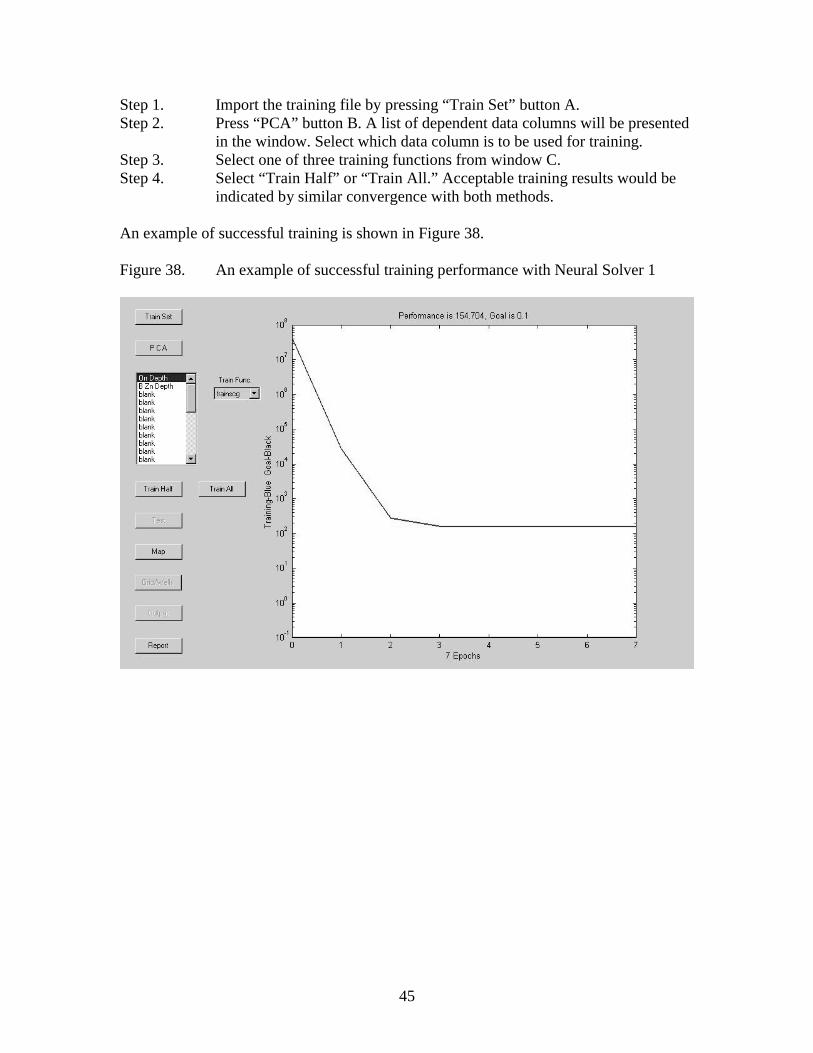
Step 1. Import the training file by pressing “Train Set” button A.Step 2. Press “PCA” button B. A list of dependent data columns will be presented

in the window. Select which data column is to be used for training.Step 3. Select one of three training functions from window C.Step 4. Select “Train Half” or “Train All.” Acceptable training results would be

indicated by similar convergence with both methods.

An example of successful training is shown in Figure 38.

Figure 38. An example of successful training performance with Neural Solver 1

46

Step 5. Press “Test” button to display the correlation plot.

An example of plot displayed after pressing the “Test” button “G” is shown in Figure 39.

Figure 39. Display of training correlation between results and dependent data fromNeural Solver 1.

Although the training performance did not achieve the goal of 0.1, a reasonablecorrelation has been achieved if the “R” correlation coefficient is satisfactory.

Step 6. Press “Map” button to apply training and create a map from theindependent data. The map will be displayed as in Figure 37.

47

If training is unsuccessful, the training performance graph will be similar to that shown inFigure 40.

Figure 40. An example of unsuccessful training performance with Neural Solver 1.

In some circumstances, training will not converge as shown in Figure 40. Try selecting adifferent training function in window box “E.” If convergence cannot be achieved withany of the 3 training functions, the training population may be too small or there isinsufficient relationship between the dependent and independent data.

48

Step 7. Export a PCA report by pressing “Report” button “K”, optional.

An example of a PCA report is shown in Figure 41.

Figure 41. An example of a PCA report from Neural Solver 1.

There are three sections to the report.

• List of the data columns from the input files which are used as input to the ANN.

• The transformation matrix obtained from PCA. If there are n data columns listedin the previous section, and PCA has reduced these to m columns, then this is an nby m matrix. Each row of input data is multiplied by this matrix to reduce it fromn to m elements.

• The weights used by the ANN. The ANN output is the dot product of theseweights with the PCA-reduced input data.

49

Step 8. Export an output file that contains the map information by pressing“Output” button “J.”

The output file contains the map information in a grid with 120 by 120 nodes. Anexample of an output file is shown in Figure 42.

Figure 42. An example of a map output file from Neural Solver 1.

x y value1252636 161860 -65631252558 161860 -65621252636 161973 -65621252558 161973 -65621252714 161748 -65611252714 161860 -65601252636 161748 -65601252558 162085 -65601252636 162085 -65591252558 162198 -65591252636 162198 -65591252480 162198 -65591252714 161973 -65591252480 161860 -6559

Practice files for the Neural Solver 1 Tool are located under the directory\tools_ann\input_files1\. Output files relating to the figures shown in this section arelocated under the directory \tools_ann\output1\.

50

TOOLS and UTILITIES

Neural Solver 2

The Neural Solver 2 routine is used to predict a parameter, that is measured at a limitednumber of locations over some x-y region, by using an ANN to relate it to a set ofattributes which are known at regular grid locations.

In normal use, the predicted parameter is some measure of well “goodness”, such asinitial production, and the attributes are the outputs from one or more other ICSprograms. All input data files are assumed to be comma-separated-variable files, withcoordinates assigned in the first two columns. The first row is reserved for column labels.There are no other assumptions about the content of the files. The user specifies trainingdata by selecting them from list boxes. An over lap of the data files is computed. Gridoperations are then applied to the data within the common area.

The ANN used in this program is a simple linear classifier (ADALINE) having oneoutput. The number of inputs is by user-selection of data columns. The input data arenormalized, but no PCA is done. The MATLAB default training function is used.

Data

Neural solver 2 can import multiple files containing independent data. The Neural Solver2 routine is intended to import the output from other ICS tools that have been used topredict reservoir parameters such as porosity-thickness, growth-history and entrapmentpressure. Data columns within each file can be selected as desired by the user. One filecontains locations and well data. The file that contains well data is the “objective” file.Objectives that are contained in this file will represent reservoir “goodness.” Quantitiesfrom production history such as initial 24-month production, oil-cut and estimatedultimate recovery are examples of “goodness.” When the Neural Solver 2 routine isutilized with these types of data, the output will be a “Z” map that has been objectivelyweighted and ranked according to the data selected from the objective file. An exampleof using the Neural Solver 2 Tool in this manner is presented in the tutorial section.

There are some advantages for using Neural Solver 2. Separate files of independent datacan be imported. These files are located in a common directory reserved for the study.The coordinates of the independent data files need not match, but there must be somecommon area. There is no need to capture the independent data at the location of thedependent data (wells). Interpolating the independent data at well locations is done by theprogram.

There are also some disadvantages for using Neural Solver 2. If the dependent data(wells) population is small, successful training may not be possible. Although there areno hard rules, the dependent data population should be more than twice the number ofindependent items (3 independent items with 6 wells). Another disadvantage is that thereis only one option for training.

51

An example of a training objective file for neural solver 2 is shown in Figure 43. The firstrow is reserved for labels. The first two columns contain x-y coordinates. The thirdcolumn contains a numeric well label. The dependent data are in the following columns.There is no limit to the number of dependent data columns. The objective file shown inFigure 43 contains sub-sea depths to the Red River Formation and Red River B zonereservoir at measured locations in a 3D seismic survey. In this case, the Neural Solver 2routine is not used to created a “Z” map of reservoir “goodness.” The example files thatfollow demonstrate, using depth as the objective, the procedure for working with theNeural Solver 2 Tool.

Figure 43. An example of an objective training file for Neural Solver 2 as viewedwith spreadsheet software.

x y Well Orr Depth B Zn Depth1254737 158993 1 -6500 -65431258348 159293 2 -6454 -64991257953 158110 3 -6401 -64431258116 158314 4 -6404 -64471258315 158463 5 -6405 -64481258702 158574 6 -6413 -64561259280 158704 7 -6437 -64801259006 157371 8 -6433 -64751257814 154290 9 -6496 -65371253880 156077 10 -6485 -65251253711 156637 11 -6490 -65301253676 157227 12 -6489 -65291253674 157422 13 -6493 -65331253675 157457 14 -6494 -65341253662 158426 15 -6489 -65291253645 158616 16 -6494 -65341253572 158894 17 -6503 -65411253603 158801 18 -6503 -65411253502 159032 19 -6505 -65431253050 159452 20 -6516 -65541254615 155311 21 -6472 -65141255263 151907 22 -6455 -64941257096 151448 23 -6436 -64761256972 151226 24 -6434 -64741256930 151043 25 -6438 -64781256883 150688 26 -6444 -64841256883 150564 27 -6448 -64881256817 150039 28 -6463 -65031256797 149908 29 -6467 -65071256747 149687 30 -6473 -65131256699 149474 31 -6477 -65171256614 149113 32 -6483 -6523

Shown in Figure 44, is an example of seismic times at important geologic horizons thathave been exported from seismic interpretation software.

52

Figure 44. An example of an input file for Neural Solver 2 that contains independentdata as viewed with spreadsheet software.

x y Ke_time Kgh_time Kmo_time Mk_time Mmc_time Dtf_time Orr_time1251925 148805 722 1064 1174 1595 1665 1775 18811251925 149132 724 1064 1174 1596 1666 1775 18811251925 149459 723 1064 1175 1598 1667 1776 18811251925 149785 726 1059 1174 1612 1667 1775 18811251925 150112 727 1059 1175 1604 1670 1776 18821251925 150439 719 1059 1177 1604 1671 1776 18821251925 150765 717 1059 1178 1604 1672 1776 18811251925 151092 717 1057 1174 1605 1672 1776 18811251925 151419 720 1059 1174 1606 1669 1777 18801251925 151745 723 1061 1173 1605 1669 1774 18791251925 152072 720 1062 1169 1605 1669 1771 18771251925 152399 716 1061 1171 1602 1670 1773 18781251925 152725 715 1060 1170 1601 1667 1772 18791251925 153052 714 1060 1170 1603 1664 1773 18771251925 153379 717 1055 1172 1606 1666 1774 18751251925 153705 717 1054 1170 1606 1668 1775 18751251925 154032 714 1056 1170 1603 1668 1775 18761251925 154359 713 1056 1168 1600 1666 1776 18771251925 154685 715 1055 1171 1599 1665 1775 18771251925 155012 716 1054 1170 1600 1666 1774 18771251625 155339 717 1053 1168 1600 1665 1774 18761251925 155339 717 1053 1168 1600 1665 1774 1876

53

An example of an exported file that contains seismic interval-times is shown in Figure45. This file is created by seismic interpretation software.

Figure 45. An example of a second input file for Neural Solver 2 that containsdifferent independent data as viewed with spreadsheet software.

x y Ke-kgh Ke-Kmo Ke-Mk Ke-Mmc Ke-Dtf Ke-Orr1251925 148805 342 452 873 943 1053 11591251925 149132 340 450 872 942 1051 11571251925 149459 341 452 875 944 1053 11581251925 149785 333 448 886 941 1049 11551251925 150112 332 448 877 943 1049 11551251925 150439 340 458 885 952 1057 11631251925 150765 342 461 887 955 1059 11641251925 151092 340 457 888 955 1059 11641251925 151419 339 454 886 949 1057 11601251925 151745 338 450 882 946 1051 11561251925 152072 342 449 885 949 1051 11571251925 152399 345 455 886 954 1057 11621251925 152725 345 455 886 952 1057 11641251925 153052 346 456 889 950 1059 11631251925 153379 338 455 889 949 1057 11581251925 153705 337 453 889 951 1058 11581251925 154032 342 456 889 954 1061 11621251925 154359 343 455 887 953 1063 11641251925 154685 340 456 884 950 1060 11621251925 155012 338 454 884 950 1058 11611251625 155339 336 451 883 948 1057 1159

54

Upon execution of the command to start the Neural Solver 2 routine, a work window ispresented as shown n Figure 46.

Figure 46. An example of the work window for Neural Solver 2 and navigation key.

Key to the work window for Neural Solver 2.

A. Select input filesB. List box displays files and data columns.C. Select objective file for training.D. List box displays the data columns contained in the objective file.E. Prepare data after making selections from input files.F. Train with highlighted objective item.G. Special training and validation feature.H. Training is applied and a map generated.I. Land grid and well locations are overlain on map.J. Map area.K. Color bar and scale.

55

Step 1 Load input files by pressing “Input Files” button”A.” These files shouldexist in a separate work directory. All files with a csv extension will beread from the work directory.

Step 2. Select independent data to be processed from the list box “B.” Use acontrol left-click to toggle the selections. Do not select the file name orcoordinates. The file name is shown with capital letters.

After the input files have been read and data columns selected, the work window forNeural Solver 2 will be similar to that shown in Figure 47.

Figure 47. The work window for Neural Solver 2 is shown after selecting directorywith the input (independent data) files.

56

Step 3. Press “Objective File” button “C.” This file should exist in a separatework directory that is different from the work directory for the input files.

Step 4. Press “Data Prepare” button “E.” All selected data will be loaded.Intersecting area of the input files will be computed. The independent data(input files) will be interpolated and placed in a work matrix. Interpolatedvalues for independent data will be captured at the well locations found inthe objective file.

After the objective file is read and data column selected, the work window for NeuralSolver 2 will be similar to that shown in Figure 48.

Figure 48. The work window for Neural Solver 2 is shown after selecting objective(dependent data) file.

Step 5. Select training objective from list box “D.”Step 6. Press “Train” button “F.”

57

After pressing the “Train” button “F”, a training performance graph is displayed asshown in Figure 49. The graph shown does not indicate convergence. The training hasfailed. If convergence does not occur, experiment with the input file selections from listbox “B.” Press “Data Prep” button again after new selections are made.

Figure 49. An example of unsuccessful training from Neural Solver 2

58

Figure 50 shows that convergence occurred after de-selection of “ke-mk” and “ke-mmc”from the independent data. It may be instructive to separately train with each independentdata column and observe the training performance. In a final run, select only thoseindependent data that produced the best performance.

Figure 50. An example of successful training from Neural Solver 2.

Step 7. Press “Run” button “H” to create a map of the training results applied tothe independent data.

Step 8. Press “Grid/Wells” button “I” to over lay the land grid and well locations.

59

Step 9. Press the “Auto” button “G”, optional.

The “Auto” option is a special feature that made that predicts parameters at each well(control point) from the remaining wells as training data. A report is generated thatcompares the measured values to the predicted values. An example of output from the“Auto” feature of the Neural Solver 2 Tool is shown in Figure 51.

Figure 51. An example of actual (a) and prediction (p) values from Neural Solver 2for the dependent data in the objective file.

WELL (a)Orr Depth (p)Orr Depth (a)B Zn Depth (p)B Zn Depth1 -6500 -6489 -6543 -65282 -6454 -6412 -6499 -64553 -6401 -6409 -6443 -64524 -6404 -6405 -6447 -64485 -6405 -6387 -6448 -64306 -6413 -6380 -6456 -64237 -6437 -6409 -6480 -64518 -6433 -6415 -6475 -64559 -6496 -6451 -6537 -6491

10 -6485 -6449 -6525 -649111 -6490 -6468 -6530 -651012 -6489 -6454 -6529 -649413 -6493 -6453 -6533 -649414 -6494 -6453 -6534 -649315 -6489 -6463 -6529 -650316 -6494 -6462 -6534 -650217 -6503 -6477 -6541 -651618 -6503 -6460 -6541 -650019 -6505 -6476 -6543 -651620 -6516 -6473 -6554 -651221 -6472 -6419 -6514 -646222 -6455 -6462 -6494 -650323 -6436 -6408 -6476 -645024 -6434 -6421 -6474 -646225 -6438 -6420 -6478 -646126 -6444 -6430 -6484 -647127 -6448 -6430 -6488 -647128 -6463 -6448 -6503 -648829 -6467 -6447 -6507 -648830 -6473 -6446 -6513 -648731 -6477 -6465 -6517 -650532 -6483 -6464 -6523 -6504

Practice files for the Neural Solver 2 Tool are located under the directory\tools_ann\input_files2\.

60

TOOLS and UTILITIES

Manual Combine

The Manual Combine Tool can produce a reservoir potential or “Z” map. Output can bearithmetically summed by supplying user-supplied weights to the data (up to seven datasources). Imported data could be output files for depositional setting and porositydevelopment, structural growth, and entrapment potential. The Manual Combine Toolprovides a subjective evaluation of reservoir potential as supplied by weights from theuser in an arbitrary fashion or as an attempt to shift weights to match the user’sknowledge of well performance. The combine tool could be also used to explore differentweighting to approximate the results computed by the neural solver.

Data

Input data for the Manual Combine Tool are created with the Cluster 1 or Cluster 2routines. An example of an output file from Cluster 1 or 2 is shown is Figure 52. Therank column (4) from the cluster output is used to characterize reservoir “goodness.” It isassumed that ranking order is the same for each input file; 1 is good and 4 is poor. Up to7 input files can be imported at one time. The files must reside in a separate directory.The routine will attempt to read each file in the work directory that has a csv extension.

Figure 52. An example of a rank file produced by Cluster 1 or Cluster 2.

x y cluster rank mean 1 mean 21205030 140303 0 0 NaN NaN1205742 153787.4 1 4 221 0.651205505 151061.9 2 3 226 5.731205505 151205.3 3 2 228 5.831205505 153213.6 4 1 229 4.68

61

After executing the command for the Manual Combine Tool, a work window is presentedas shown in Figure 53.

Figure 53. An example of the work window for Manual Combine and navigation key.

Key to work window for the Manual Combine Tool.

A. Load input files.B. List box showing files and data columns.C. Prepare button overlays and merges data.D. Apply weights to selected data.E. Overlay land grid and well locations, optional.F. Map area.G. Color bar and scale.

Step 1. Load input files by pressing “Files” Button “A.”Step 2. Select data columns from list box “B.”Step 3. Press “Prepare” button “C.”Step 4. Press “Combo” button “D.” A second work window is presented.

62

After pressing the “Combo” button “D”, a new window is presented as shown in Figure54. In general use, the weights will be from 0 to 1. Leaving all weights to a value of 1will give each input file equal value.

Figure 54. An example of the second work window for the Manual Combine Tooland navigation key.

Key to second work window for Manual Combine Tool.

H. List box of selected data columns and weights to be applied.

Step 5. Change weights as desired. A zero will remove item from summation.Close the window and a new map will be created with the suppliedweights.

63

A “Z” map is computed from the user-supplied weights and the selected data as shown inFigure 55.

Figure 55. An example from Manual Combine Tool with different weights applied toinput data.

The areas with low values are good. Large values indicate poor ranking from selecteddata and weights. In this example there are 3 input files. Areas with a value of 3 representregions where the 3 input files have a rank of 1 (best).

64

TOOLS and UTILITIES

Fuzzy Combine

The Fuzzy Combine Tool is a form of “expert system” used to consistently apply rulesfor characterization of reservoir potential. This tool relies for its operation on a fuzzyinference system (FIS) built with the MATLAB Fuzzy Editor. A MATLAB FIS is asingle file (with extension .fis) which contains the definition of a complete fuzzyinference system, consisting of input variable membership functions, fuzzy rules, andoutput variable mapping functions. The FIS editor provides for the definition and editingof these components with a simple GUI. See the MATLAB Fuzzy Logic Toolbox User’sGuide for details. This documentation can be found on the MATLAB web site.

The ICS Fuzzy Combine Tool is a control and display shell around the FIS, which allowsthe user to select data files for input to the FIS, and displays the FIS output in map formconsistent with the other ICS tools.

In general use, the user will define a FIS external to ICS. The FIS may have any numberof inputs and rules, and should have one output. For use in ICS as a combine tool, theinputs are presumably data that are created by other ICS tools. The rules relate values ofthese reservoir characterization parameters to some overall measure of reservoirpotential, which is the mapped output.

In its demonstration form supplied here, the tool applies rules to 2 reservoir parameters:entrapment pressure and porosity-thickness (phi-h) for a particular reservoir in the UpperRed River. The entrapment pressure is output from the Entrapment Tool, and thepredictions of phi-h are made with a neural solver, cluster tool or multiple-linearregression tool. The 2-input FIS for this case is called drules2.fis. Demonstration files forthe example shown in Figure 56 are located under the directory \tools_fuzzy\input_files\.

The Fuzzy Combine Tool is under development and is not ready for a tutorial example atthis time. After further calibration and sophistication are incorporated in this tool, weplan to post an update and tutorial example on the project web site. It is anticipated thatthis will be accomplished in the first quarter of 2002.

65

Shown in Figure 56 is the work window and navigation key for the “Fuzzy Combine”tool.

Figure 56. Work window for Fuzzy Combine Tool and navigation key.

Navigation key for Fuzzy Combine Tool.

A. Load input files. Input files must reside in a separate directory.B. Select one data column. Press “Add.” Column name is copied to window “D.”

Repeat for second data column.C. Copies column name selected from “B” to “D.”D. Window containing data for fuzzy rules. Entrapment is first, phi-h is second.E. Clear button to start over with file selection.F. Press “Prepare” button after data are selected. Overlay and grid operations begin.G. Map is displayed of data item that is highlighted in window “D.”H. File name of fuzzy rules that apply to the data selected.I. “Test” button applies fuzzy rules and creates a map in window “K.”J. Overlay land grid and well locations from a special file.K. Map area.L. Color bar and scale. Scale is from 0 to 100. A score of 100 is the best possible.

66

Shown in Figure 57 is an example of entrapment-pressure input as mapped by the “FuzzyCombine” tool.

Figure 57. An example of entrapment-pressure input as mapped by the FuzzyCombine Tool.

Shown in Figure 58 is an example of porosity-thickness input as mapped by the “FuzzyCombine” tool.

Figure 58. An example of porosity-thickness input as mapped by the Fuzzy CombineTool.

67

Shown in Figure 59 is an example of output from application of fuzzy rules with the“Fuzzy Combine” tool.

Figure 59. Final output from application of rules with Fuzzy Combine Tool.

The score from application of the fuzzy rules (item box “H”) is shown on the color bar. Ascore of 100 is the maximum “goodness.” A score of “0” is the minimum “goodness.”

68

TUTORIALS

Introduction

Software tools in ICS are for evaluating various data sets from seismic, geologic andengineering sources. The objective of these tools is to provide a means for logical andconsistent reservoir characterization. These tools can be broadly characterized as 1)clustering tools, 2) neural solvers, 3) multiple-linear regression, 4) entrapment-potentialcalculator and 5) combining tools. A flexible approach can be used with the ICS tools.They can be used separately or in a series to make predictions about some objective.

The tools in ICS are primarily designed to correlate relationships between seismicinformation and data obtained from wells. It is possible to work with well data alone.Likewise, there may be special circumstances where seismic data could used without welldata. A generalized approach to reservoir characterization with ICS is shown in Figure60.

Figure 60. ICS Data and Logic flow.

DATA →→→→ TOOLS →→→→INTERMEDIATEOBJECTIVES →→→→ COMBINE →→→→ “Z” MAP

Formation Tops Clustering Deposition Manual Weight ReservoirLog Analysis Neural Solver Structure Neural Solver PotentialProduction Linear Regression Growth History Fuzzy RulesFlow Tests StorageSeismic Time TransmissibilitySeismic Intervals Fluid SaturationSeismic Attributes EntrapmentSeismic Models

An example of data and approach for evaluation of depositional setting is shown inFigure 61.

Figure 61. Data and logic flow for depositional setting.

DEPENDENTDATA →→→→

INDEPENDENTDATA →→→→ TOOLS →→→→ OBJECTIVE →→→→ OUTPUT

Rock Quality Micro Intervals Clustering Intervals Rank- meanPorosity Formation-marker Correlating File and mapPermeability Tops/Picks To rock qualityFacies From well logs Rock type orShale Volume Facies

69

An example of data and approach for evaluation of structure and growth history is shownin Figure 62.

Figure 62. Data and logic flow for structure and growth history.

DEPENDENTDATA →→→→

INDEPENDENTDATA →→→→ TOOLS →→→→ OBJECTIVE →→→→ OUTPUT

Production Macro Intervals Clustering Rank Rank- meanOil volume Formation-marker Interval patterns File and mapProduction rate Tops/Picks With productionOil cut From well logs With depthReservoir depth From Seismic

Neural Solver Transform ProductionInterval patterns AttributeTo production File and mapRelated values

An example of data and approach for transformation of seismic attributes to reservoirattributes is shown in Figure 63.

Figure 63. Data and logic flow for seismic pseudo-reservoir attributes.

DEPENDENTDATA →→→→

INDEPENDENTDATA →→→→ TOOLS →→→→ OBJECTIVE →→→→ OUTPUT

Reservoir attributes Seismic attributes Clustering Reservoir Rank- meanAt wells Amplitude Attributes File and mapThickness Frequency At seismicStorage Isochron TracesPorosityTransmissibility Neural Solver TransformedPermeability Seismic

AttributesFile and map

Multiple TransformedLinear SeismicRegression Attributes

File and map

70

An example of data and approach for transformation of seismic attributes to reservoirfluid saturation is shown in Figure 64.

Figure 64. Data and logic flow for fluid saturation.

DEPENDENTDATA →→→→

INDEPENDENTDATA →→→→ TOOLS →→→→ OBJECTIVE →→→→ OUTPUT

Reservoir attributes Special Seismic Clustering Reservoir Rank- meanAt wells Attributes Attributes File and mapWater saturation Frequency At seismicOil cut AVO TracesPorosity Water saturation

Oil cutNeural Solver Transformed

SeismicAttributesFile and map

An example of data and approach for estimating entrapment potential for a reservoir isshown in Figure 65.

Figure 65. Data and logic flow for entrapment.

DEPENDENTDATA →→→→

INDEPENDENTDATA →→→→ TOOLS →→→→ OBJECTIVE →→→→ OUTPUT

Reservoir attributes Reservoir depth Entrapment Structure and EntrapmentAt wells Stratigraphic PotentialWater density Cluster rank file Potential File and mapCapillary properties Porosity orDatum pressure permeability

71

An example of data and approach for combining results from intermediate objectives isshown in Figure 66.

Figure 66. Data and logic flow for final objective.

DEPENDENTDATA →→→→

INDEPENDENTDATA →→→→ TOOLS →→→→ OBJECTIVE →→→→ OUTPUT

Reservoir attributes Transformed Manual combine Subjective SummationAt wells Seismic attributes Weights ForStorage RelativeTransmissibility Storage GoodnessEntrapment TransmissibilityOil cut Growth historyOil rate Entrapment Neural Solver Objective DirectUltimate recovery Weights Prediction

From trainingOil-cutOil rateEUR

Fuzzy rules Objective ConsistentWeights Rules For

RelativeGoodness

Data

Data should be collected and organized that are appropriate for intermediate objectives.Some suggested reservoir characterization items from well data are listed below.

A. A model for reservoir deposition and genesis should be developed. In general, thedepositional setting can be inferred from various intervals within and near thereservoir objective. Appropriate data would include formation or marker-beddepths.

B. Most reservoirs have some component of structural trapping. Appropriate datawould be the depth to the reservoir objective. In some instances, especially withseismic time, structure may be expressed as an interval from a shallow horizon tothe reservoir objective.

C. Growth history describes the evolution of structure. Appropriate data would beimportant formation tops from surface to some formation or marker-bed belowthe reservoir objective. A suggested number of formation depths for this data setwould be five or six.

72

D. Storage is porosity-thickness. The data will come from analysis of well logs. Thedata set will summarize gross thickness, net gross thickness and effectiveporosity-thickness for the reservoir objective.

E. Transmissibility is a property that describes flow capacity. Permeability-thicknessor draw-down indices are possible parameters that describe flow capacity. Drill-stem tests, production-curve analysis and back-pressure tests are good sources forthis characterization item.

F. Fluid saturation in the reservoir can be characterized from well-log analysis andproduction data.

The data should be entered into spreadsheets and organized in the manner shown in thefollowing tables. The spreadsheets must be saved or exported in comma-separated-variable format. The first two columns are reserved for coordinates in any cartesian firstquadrant format. The first row is reserved for data labels. Do not have more than one rowof labels.

Construction of a database for dependent well information should be the first order ofbusiness. The file will contain numeric values of items that describe the quality of thereservoir as shown in Figure 67.

Figure 67. An example of a data file containing reservoir parameters from wellinformation.

EAST NORTH WELL Storage DST Oil-cut Transmissibility BOPD Avg. Oil-cut Avg.FT FT API No. PHI-H Fraction KH 24 months 24 months

1212611 154710 3301100198 1.770 0.600 8.511214184 150850 3301100258 0.578 2.521214039 147068 3301100259 0.908 1.000 10.31 112.5 0.6011212821 149427 3301100262 1.349 0.983 33.49 60.3 0.7361212031 153869 3301100305 0.990 74.3 0.9371213827 150045 3301100311 1.130 0.938 85.70 79.8 0.9811207014 152537 3301100339 1.569 0.088 0.29 0.0 0.0881215767 142373 3301100343 1.734 0.949 19.47 14.3 0.4151212374 144767 3301100432 1.248 0.082 2.631212474 145067 3301100488 1.196 0.120 5.041211646 144209 3301100915 0.929 0.470 15.10 42.0 0.5001257953 158110 3301100195 0.918 0.938 24.06 141.9 0.9801254615 155311 3301100200 1.485 1.000 121.17 118.6 0.6881257096 151448 3301100208 1.824 1.000 329.83 162.8 0.9831257814 154290 3301100254 1.511 0.071 63.38 0.0 0.0001251775 148752 3301100297 1.117 0.660 67.55 32.5 0.7641252062 153191 3301100356 1.817 0.005 170.62 0.0 0.0001254737 158993 3301100423 1.977 0.217 199.631251493 151452 3301100452 1.634 0.048 120.06 0.0 0.0001255263 151907 3301100458 1.389 0.000 8.12 74.2 0.6541259006 157371 3301100819 1.060 0.613 86.16 95.0 0.5241258348 159293 3301100865 0.812 0.000 75.77 49.5 0.4641253880 156077 33011009401283178 124373 3301100182 0.691 0.620 26.28 52.7 0.944

73

It is recommended to construct a database of geologic tops related to depositional setting.These data are obtained from well logs. An example data file of geologic tops related todepositional setting is shown in Figure 68.

Figure 68. An example data file of geologic tops related to depositional setting.

EAST NORTH WELL Red River A Zone B Zone C Zone D Zone BaseFT FT API NO. Depth Depth Depth Depth Depth Depth

1212611 154710 3301100198 -6216 -6225 -6256 -6306 -6398 -64431214184 150850 3301100258 -6217 -6226 -6255 -6303 -6385 -64341214039 147068 3301100259 -6189 -6198 -6225 -6271 -6363 -64111212821 149427 3301100262 -6202 -6213 -6241 -6284 -6380 -64271212031 153869 3301100305 -6218 -6227 -6258 -6305 -6398 -64451213827 150045 3301100311 -6186 -6194 -6222 -6267 -6366 -64001207014 152537 3301100339 -6250 -6259 -6290 -6336 -6429 -64761215767 142373 3301100343 -6204 -6214 -6243 -6293 -6387 -64351212374 144767 3301100432 -6179 -6188 -6217 -6265 -6359 -64071212474 145067 3301100488 -6189 -6199 -6229 -6277 -6369 -64181211646 144209 3301100915 -6192 -6202 -6231 -6277 -6370 -64181257953 158110 3301100195 -6401 -6407 -6443 -6487 -6586 -66231254615 155311 3301100200 -6472 -6481 -6514 -6558 -6652 -66991257096 151448 3301100208 -6436 -6442 -6476 -6522 -6616 -66621257814 154290 3301100254 -6496 -6505 -6537 -6588 -6683 -67341251775 148752 3301100297 -6446 -6455 -6488 -6533 -6627 -66751252062 153191 3301100356 -6475 -6482 -6517 -6565 -6660 -67091254737 158993 3301100423 -6500 -6509 -6543 -6594 -6690 -67401251493 151452 3301100452 -6465 -6473 -6508 -6555 -6653 -6701

74

For evaluation of structure and growth history, a database should be constructed fromwell logs that contains sub-sea depths to important geologic formations. An example datafile of geologic tops related to structural growth is shown in Figure 69.

Figure 69. An example data file of geologic tops related to structural growth.

EAST NORTH WELL Kn Kmo Km Mmc Si OrrFT FT API NO. Depth Depth Depth Depth Depth Depth

1212611 154710 3301100198 -158 -1233 -3298 -4476 -5706 -62161214039 147068 3301100259 -128 -1234 -3281 -4442 -5677 -61891212821 149427 3301100262 -135 -1232 -3269 -4455 -5698 -62021212031 153869 3301100305 -152 -1233 -3301 -4478 -5714 -62181213827 150045 3301100311 -144 -1247 -3263 -4446 -5676 -61861207014 152537 3301100339 -130 -1236 -3352 -4487 -5723 -62501215767 142373 3301100343 -144 -1268 -3262 -4447 -5680 -62041212374 144767 3301100432 -127 -1246 -3252 -4426 -5662 -61791212474 145067 3301100488 -130 -1236 -3267 -4439 -5668 -61891211646 144209 3301100915 -140 -1249 -3262 -4440 -5672 -61921257953 158110 3301100195 -274 -1335 -3296 -4528 -5834 -64011254615 155311 3301100200 -275 -1347 -3325 -4558 -5868 -64721257096 151448 3301100208 -278 -1342 -3301 -4531 -5852 -64361257814 154290 3301100254 -287 -1349 -3319 -4567 -5895 -64961251775 148752 3301100297 -269 -1330 -3312 -4533 -5846 -64461252062 153191 3301100356 -276 -1339 -3305 -4557 -5864 -64751254737 158993 3301100423 -279 -1348 -3388 -4572 -5895 -65001251493 151452 3301100452 -270 -1325 -3312 -4546 -5859 -64651255263 151907 3301100458 -272 -1341 -3310 -4532 -5858 -64551259006 157371 3301100819 -272 -1334 -3308 -4539 -5852 -64331258348 159293 3301100865 -279 -1340 -3303 -4543 -5864 -6454

75

A database of seismic attributes that are (or could be) related to reservoir variation shouldbe constructed from exported files from seismic interpretation software. Such a file isshown in Figure 70.

Figure 70. An example data file of seismic attributes related to the reservoirobjective.

EAST NORTH P1max T1min P2max P1-Owiz T1-Owiz P2-OwizFT FT Amplitude Amplitude Amplitude msec msec msec

1216902 153434 6448 -2981 5018 64 57 371216455 152997 5203 -3072 4325 62 56 401216902 152997 6596 -2643 4337 63 57 381216455 153434 6003 -5684 6791 63 58 381216455 153872 5075 -5896 6688 65 57 391216455 154310 6344 -6037 7764 64 58 411216009 151683 7162 -7228 5456 63 56 381216902 152559 6827 -4617 6755 65 58 401216009 152997 6640 -4657 4144 65 59 401216902 152121 5004 -4457 6181 64 57 391216009 152121 6358 -8845 7009 66 59 381216455 151683 7173 -6478 4800 63 56 381216455 152121 4778 -9348 6518 64 57 391216009 152559 6987 -7869 5809 61 56 391216455 152559 5886 -7840 5346 63 57 401214668 157374 8032 -4073 7298 64 56 371216902 151683 5088 -2911 5653 62 55 361216009 153434 5240 -9732 6367 64 58 391216009 153872 6019 -6218 7329 64 58 39

76

For evaluation of structure and growth history, a database should be constructed fromseismic that contains reflection time at important geologic formations. These data areexported files from seismic interpretation software. An example data file of seismic timepicks related to structural growth is shown in Figure 71.

Figure 71. An example data file of seismic time picks at important geologic horizons.

EAST NORTH Ke Kn Kgh Mmc Orr OwiFT FT msec msec msec msec msec msec

1207727 148819 635 854 984 1612 1803 18591206414 148488 636 855 983 1610 1803 18591209040 148488 636 852 982 1613 1801 18571206414 148819 636 856 984 1613 1804 18591206742 148488 636 854 982 1609 1803 18591207070 149482 637 856 987 1617 1805 18601208055 148819 637 852 983 1614 1802 18581210025 144847 637 857 988 1613 1800 18561211338 145840 637 854 987 1612 1799 18551207727 148488 637 853 984 1612 1802 18591206742 148157 637 854 983 1608 1803 18591207070 148157 638 854 983 1608 1803 18591207398 148819 638 855 985 1616 1804 18601207398 148157 638 853 984 1610 1803 18601208712 148819 638 853 983 1614 1802 18571209040 148157 638 852 982 1613 1799 18561210025 147164 638 853 984 1611 1800 18561210353 146171 638 852 983 1610 1799 18551210025 144516 638 855 990 1613 1800 18561205757 152792 638 855 983 1619 1807 18641208712 149482 638 854 985 1617 1804 18591207070 149150 638 855 985 1616 1805 1861

77

Getting Started

It is recommended to start with a 3D seismic data set and use the Cluster 3 tool. A simpleseismic data set would consist of two-way travel time and interval time at major seismicreflectors or important geological horizons. Cluster 3 requires no well data as it producesnatural or intrinsic clusters without correlation to any reservoir or physical property.

After producing cluster maps with time and interval time, proceed to experimenting,again with Cluster 3, with seismic attributes (such as amplitude) at the reservoirobjective.

Next, create a file to use with the Cluster 1 tool. Start simple and use two-way travel timeat major seismic reflectors as the independent data. Make a file of geologic intervals(corresponding to the seismic reflectors) from well logs (dependent data) that areavailable within the 3D seismic survey area. Merge the two files after the seismic two-way travel time has been supplied for the well locations. Create cluster maps for seismictwo-way travel time and interval thickness from well logs. Observe which seismic timeintervals correlate best with well-log interval thickness. Compare cluster maps fromCluster 1 to those produced by Cluster 3.

After becoming comfortable with Cluster 1, begin experimenting with the Cluster 2 tool.Make a dependent-data file of simple reservoir properties from the wells located withinthe 3D seismic survey. Include reservoir properties such as thickness, porosity-thicknessand average porosity. Create an independent-data file from simple seismic informationsuch as maximum peak and minimum trough amplitudes near the reservoir objective.Merge the two files after the seismic information has been supplied for the well locations.Create cluster maps for seismic information and reservoir properties from well logs.Observe which seismic attributes correlate best with reservoir properties. Comparecluster maps from Cluster 2 to those produced by Cluster 3.

Following a few sessions with the clustering tools, it is suggested to work with theEntrapment Tool. The Entrapment tool requires familiarity with output created by Cluster1 and Cluster 2 tools.

The next step is to use the neural solvers. If the suggested steps described above arefollowed, the user should acquire a better understanding of the independent seismic dataand relationships with the dependent well data. Successful use of the neural solvers, inmost reservoir characterization problems, involves selecting or screening data thatprobably have a high correlation to the reservoir attribute or objective. This is especiallynecessary when the control or well population is small. It some cases, the well populationmay be too small for using neural solvers.

After using different techniques and data sets to make predictions for several reservoircharacteristics, the user should develop a sense as to what factors are important and canbe predicted for the reservoir. Once this is achieved, the user can combine these reservoirelements through application of three combining tools.

78

TUTORIALS

Example 1

In example 1, we will use data from a 3D seismic survey in Bowman County, NorthDakota. The survey area has 9 wells for control. The example will emphasize clustering,as the clustering tools are robust and produce quick results with a small controlpopulation. We will make various cluster maps for depositional setting, porosity andstructure. The output will be combined to produce a “Z” map or potential map. Thepractice files for example 1 are located under the directory \example_1\input_files\.

The first data set includes seismic attributes within the Upper Red River. A portion of thisdata file is shown in Figure 72

Figure 72. Portion of input data file 1 used in tutorial example 1.

east north P1amp_norm T1amp_norm P2amp_norm T2amp_norm P1max-Owiz_n T1z-Owiz_normT1min-Owiz_noP2max-Owiz_n T2min-Owiz_no1211646 144209 1.31120 -1.07060 1.15990 -0.40780 0.53910 0.52360 0.56370 0.53650 0.431501212474 145067 0.92050 -0.76770 0.70980 -0.27930 0.50350 0.45110 0.65560 0.59370 0.417901212374 144767 1.01780 -0.92930 0.80690 -0.32100 0.53460 0.50970 0.55100 0.52270 0.404701215767 142373 1.18840 -0.94600 0.79960 -0.23520 0.55440 0.53100 0.54830 0.33240 0.459901207014 152537 1.11600 -1.10620 0.81000 -0.02200 0.33260 0.28620 0.21850 0.34990 0.529901213827 150045 0.73520 -0.31820 0.59680 -0.21650 0.18330 0.09050 0.52450 0.56800 0.333701212031 153869 0.90270 -0.56280 0.86150 -0.20400 0.55940 0.49150 0.57730 0.49850 0.420301212821 149427 1.04380 -0.24690 0.49140 -0.10180 0.54140 0.34090 0.56100 0.35590 0.364301214039 147068 0.85860 -0.55220 0.65220 -0.07130 0.47180 0.48380 0.48260 0.40910 0.456501214184 150850 0.58930 -0.36430 0.62930 0.12660 0.38940 0.21150 0.33200 0.09840 0.242101212611 154710 0.76230 -0.63470 0.69910 -0.32530 0.41480 0.34250 0.44840 0.31220 0.374801208412 146869 1.24110 -0.53320 0.43900 -0.22670 0.57260 0.65670 0.72680 0.91660 1.000001208412 146431 0.84210 -0.30020 0.74640 -0.32580 0.59210 0.60990 0.61450 0.81390 1.000001208859 146869 0.87420 -0.76480 0.59090 0.07390 0.53090 0.71170 0.68650 0.96500 1.000001208859 146431 0.77810 -0.16070 0.65290 -0.51620 0.70520 0.70830 0.55980 0.86200 1.000001208412 147306 1.14520 -0.60710 0.79840 -0.11120 0.60970 0.70940 0.72350 0.86870 0.877201212880 145118 1.24240 -0.97770 0.79310 -0.57290 0.39450 0.55290 0.55790 0.66460 0.584801208859 145993 0.58930 -0.21920 0.98340 -0.70720 0.63910 0.62900 0.52500 0.71990 0.940501213774 147306 0.78400 -0.60040 0.51000 -0.18820 0.48110 0.50630 0.42490 0.47100 0.570901214668 147744 0.83830 -0.98010 0.74950 -0.28210 0.40330 0.42990 0.56820 0.46150 0.557201209305 145993 0.68860 -0.31420 0.79540 -0.67800 0.79690 0.90950 0.74740 0.87170 0.885001213327 147306 0.83280 -0.50590 0.83570 -0.31960 0.55460 0.50570 0.84560 0.87430 0.470601214221 146431 1.31390 -1.38410 1.10610 -0.66490 0.54810 0.54980 0.43240 0.36770 0.272501213774 146869 0.94250 -0.62930 0.90390 -0.10060 0.60300 0.62560 0.72570 0.60110 0.455801213327 146869 0.80850 -0.62840 0.76090 0.05200 0.60630 0.64260 0.76840 0.74650 0.690601213774 146431 1.05540 -0.93210 1.04020 -0.43610 0.52590 0.47470 0.40730 0.30980 0.315601209752 147306 1.03640 -1.01930 1.01190 -0.18770 0.54550 0.70120 0.66390 0.67560 0.688201209752 146431 0.85290 -0.16070 0.92570 -0.53450 0.76800 0.82190 0.90080 0.71990 0.600601210646 143805 1.15870 -0.89860 0.87970 -0.76390 0.58210 0.55300 0.56080 0.56710 0.438201211540 145118 1.16530 -0.92360 1.14060 -0.34310 0.55060 0.61490 0.50550 0.55450 0.514101212880 146431 1.12340 -0.69130 0.80470 -0.27740 0.51560 0.60210 0.62090 0.63480 0.557501211540 145556 0.91070 -0.62440 1.06190 -0.26310 0.60950 0.53030 0.44710 0.53030 0.492501210199 147306 0.99430 -0.58630 1.03550 -0.34380 0.50680 0.49100 0.45050 0.56410 0.640401213774 147744 0.77620 -0.46680 0.62720 -0.36460 0.42110 0.35710 0.47500 0.43050 0.32640

Data file, “data_set_01.csv”, contains coordinates in the first two columns. Columns 3through 6 contain amplitude attributes. Columns 7 through 11 contain isochron data.These seismic attributes were found to respond to variation of Red River developmentfrom seismic modeling and empirical observation. The first step is to cluster these datawith Cluster 3 tool. This tool will produce from 2 to 10 clusters. Since the data are notcorrelated with any well data, this tool produces natural clusters. The patterns that areproduced will represent areas that are seismically similar. Examples of maps produced bythe Cluster 3 Tool are shown in Figures 73 , 74 and 75.

79

Figure 73. A map created by Cluster 3 with 9 cluster groups for seismic attributesused in example 1.

Figure 74. A map created by Cluster 3 with 6 cluster groups for seismic attributesused in example 1.

80

Figure 75. A map created by Cluster 3 with 3 cluster groups for seismic attributesused in example 1.

Changing the number of clusters will give the user a feel for the dominant clusters. Thedifferent cluster areas are related to changes in thickness and impedance. They are alsoprobably related to reservoir heterogeneity. The cluster maps do not provide usinformation about the reservoir. The cluster assignments are arbitrary and the order hasno meaning.

Reservoir attributes can be assigned to the seismic clusters with the Cluster 1 and 2 tools.We will do this with the Cluster 2 tool and use the same data as used previously exceptthree columns are inserted before the independent seismic data. A portion of the input filefor use with the Cluster 2 Tool is shown in Figure 76.

81

Figure 76. Portion of input data file 2 used in tutorial example 1.

east north API Orr-GM D PHI-H P1amp_norm T1amp_norm P2amp_norm T2amp_norm P1max-Owiz_n T1z-Owiz_normT1min-Owiz_noP2max-Owiz_no1211646 144209 3301100915 226.0 5.729 1.31120 -1.07060 1.15990 -0.40780 0.53910 0.52360 0.56370 0.536501212474 145067 3301100488 228.5 7.679 0.92050 -0.76770 0.70980 -0.27930 0.50350 0.45110 0.65560 0.593701212374 144767 3301100432 228.0 7.931 1.01780 -0.92930 0.80690 -0.32100 0.53460 0.50970 0.55100 0.522701215767 142373 3301100343 230.8 6.404 1.18840 -0.94600 0.79960 -0.23520 0.55440 0.53100 0.54830 0.332401207014 152537 3301100339 226.1 3.155 1.11600 -1.10620 0.81000 -0.02200 0.33260 0.28620 0.21850 0.349901213827 150045 3301100311 213.6 0.000 0.73520 -0.31820 0.59680 -0.21650 0.18330 0.09050 0.52450 0.568001212031 153869 3301100305 227.2 0.512 0.90270 -0.56280 0.86150 -0.20400 0.55940 0.49150 0.57730 0.498501212821 149427 3301100262 225.2 1.058 1.04380 -0.24690 0.49140 -0.10180 0.54140 0.34090 0.56100 0.355901214039 147068 3301100259 221.8 2.543 0.85860 -0.55220 0.65220 -0.07130 0.47180 0.48380 0.48260 0.409101214184 150850 3301100258 216.9 0.58930 -0.36430 0.62930 0.12660 0.38940 0.21150 0.33200 0.098401212611 154710 3301100198 227.7 0.899 0.76230 -0.63470 0.69910 -0.32530 0.41480 0.34250 0.44840 0.312201208412 146869 99896 1.24110 -0.53320 0.43900 -0.22670 0.57260 0.65670 0.72680 0.916601208412 146431 99894 0.84210 -0.30020 0.74640 -0.32580 0.59210 0.60990 0.61450 0.813901208859 146869 99893 0.87420 -0.76480 0.59090 0.07390 0.53090 0.71170 0.68650 0.965001208859 146431 99892 0.77810 -0.16070 0.65290 -0.51620 0.70520 0.70830 0.55980 0.862001208412 147306 99891 1.14520 -0.60710 0.79840 -0.11120 0.60970 0.70940 0.72350 0.868701212880 145118 99890 1.24240 -0.97770 0.79310 -0.57290 0.39450 0.55290 0.55790 0.664601208859 145993 99889 0.58930 -0.21920 0.98340 -0.70720 0.63910 0.62900 0.52500 0.719901213774 147306 99887 0.78400 -0.60040 0.51000 -0.18820 0.48110 0.50630 0.42490 0.471001214668 147744 99886 0.83830 -0.98010 0.74950 -0.28210 0.40330 0.42990 0.56820 0.461501209305 145993 99885 0.68860 -0.31420 0.79540 -0.67800 0.79690 0.90950 0.74740 0.871701213327 147306 99884 0.83280 -0.50590 0.83570 -0.31960 0.55460 0.50570 0.84560 0.874301214221 146431 99883 1.31390 -1.38410 1.10610 -0.66490 0.54810 0.54980 0.43240 0.367701213774 146869 99882 0.94250 -0.62930 0.90390 -0.10060 0.60300 0.62560 0.72570 0.60110

File “data_set_02.csv” provides information about the thickness of the upper Red Riverand porosity development in the D Zone. This file is imported into the Cluster 2 routine.Four cluster groups are created and ranked according to Upper Red River thickness. Theoutput map is shown in Figure 77.

Figure 77. Cluster map created by Cluster 2 of Upper Red River thickness fromseismic attributes used in example 1.

The cluster results are output to file named “data_set_02_dump.csv”

82

Similarly, “data_set_03.csv” is processed with Cluster 2. Four cluster groups are createdand ranked according to Red River D Zone porosity-thickness. Figure 78 shows theresulting cluster map.

Figure 78. Cluster map created by Cluster 2 of Red River D Zone porosity-thicknessfrom seismic attributes used in example 1.

The cluster results are output to file named “data_set_03_dump.csv”

We have now created two files that represent a correlation with seismic attributes fordepositional setting and porosity. The cluster maps created with Cluster 2 should becompared to those created with Cluster 3. By doing so, it should be apparent that theareas of similar natural clusters have meaningful relationships with Red River reservoirdevelopment.

Data file “data_ set_04.csv” contains seismic time and interval picks for 9 events fromthe Cretaceous through Ordovician. A portion of this file is shown in Figure 79.

83

Figure 79. Portion of input data file 4 used in tutorial example 1.

x y Ke_time Kn_time Kgh_time Kmo_time Mk_time Mmc_time Dtf_time T1z_time Owiz_time1205757 150806 643 858 989 1116 1552 1620 1708 1807 18631205757 151137 644 859 989 1113 1552 1621 1708 1808 18631205757 151468 643 858 988 1112 1551 1620 1709 1808 18631205757 151799 642 857 987 1112 1551 1618 1711 1809 18621205757 152130 640 857 986 1110 1548 1618 1711 1809 18631205757 152461 639 857 985 1111 1551 1619 1709 1808 18641205757 152792 638 855 983 1113 1551 1619 1711 1807 18641205757 153123 638 855 984 1114 1551 1619 1715 1807 18631205757 153454 641 856 984 1114 1544 1620 1711 1807 18621205357 151799 642 857 987 1112 1551 1618 1711 1809 18621204957 151799 642 857 987 1112 1551 1618 1711 1809 18621206085 150475 642 858 990 1117 1552 1619 1706 1807 18621206085 150806 642 858 990 1116 1551 1619 1708 1807 18631206085 151137 643 859 989 1114 1551 1620 1709 1808 18631206085 151468 642 858 988 1113 1553 1620 1708 1808 18621206085 151799 640 857 987 1113 1552 1619 1710 1808 18621206085 152130 641 855 986 1112 1550 1620 1713 1807 18611206085 152461 641 855 983 1116 1546 1618 1713 1807 1862

We will use “data_set_04.csv” data to describe structure and structural growth. Cluster 3is used to produce natural clusters of the seismic time and intervals. A map of 9 clustergroups is shown in Figure 80. These clusters represent patterns of structure and growththat occurred between Ordovician and Cretaceous time.

Figure 80. A map created by Cluster 3 with 9 cluster groups for seismic time used inexample 1.

84

We will now assign some geological and engineering meaning to these natural patterns.Data file “data_set_05.csv” contains the same information as “data_set_04.csv” exceptthat well information is inserted in columns 3 through 5 (Figure 81). The wellinformation is the thickness between the Red River, Niobrara and Mission Canyon.

Figure 81. Portion of input data file 5 used in tutorial example 1.

x y API orr-kn orr-mmc Ke Kn Kgh Kmo Mk Mmc Dtf T1z Owiz1212611 154710 3301100198 -6058 -1740 655 862 993 1118 1551 1618 1711 1802 18551212031 153869 3301100305 -6066 -1740 652 862 992 1117 1552 1616 1709 1799 18541213827 150045 3301100311 -6042 -1741 656 862 995 1123 1559 1620 1714 1806 18571214039 147068 3301100259 -6061 -1747 652 859 989 1117 1547 1611 1705 1797 18521212821 149427 3301100262 -6067 -1747 652 859 991 1120 1554 1618 1713 1805 18581212474 145067 3301100488 -6059 -1751 645 855 989 1118 1546 1612 1707 1799 18541211646 144209 3301100915 -6052 -1752 642 856 993 1118 1548 1613 1708 1799 18541212374 144767 3301100432 -6052 -1753 643 854 990 1117 1547 1612 1707 1798 18531215767 142373 3301100343 -6060 -1757 652 863 997 1126 1553 1615 1713 1801 18561214184 150850 3301100258 -1759 660 864 996 1125 1561 1623 1713 1807 18591207014 152537 3301100339 -6120 -1762 643 855 984 1117 1551 1614 1703 1803 18561216262 152792 95 -6185 -1831 666 872 1005 1129 1568 1635 1738 1831 18881207727 148819 1555 635 854 984 1112 1545 1612 1708 1803 18591206414 148488 1554 636 855 983 1115 1541 1610 1710 1803 18591209040 148488 1553 636 852 982 1108 1554 1613 1708 1801 18571206414 148819 1552 636 856 984 1116 1544 1613 1712 1804 18591206742 148488 1551 636 854 982 1114 1539 1609 1709 1803 18591207070 149482 1550 637 856 987 1118 1551 1617 1715 1805 18601208055 148819 1549 637 852 983 1113 1548 1614 1710 1802 18581210025 144847 1548 637 857 988 1119 1552 1613 1706 1800 1856

Cluster1 is used with “data_set_5.csv” to produce three cluster groups, as shown inFigure 82. These cluster groups represent areas of similar structural growth history. Thethinnest areas, with maximum growth, are ranked as 1.

Figure 82. Cluster map of Niobrara -Red River thickness from seismic time.

85

Note that the data file uses a negative value with the interval thickness in Figure 81. Wewant the greatest value to have a rank of one. An output file is saved to “data_set_05_dump.”

Figure 83. Portion of input data file 6 used in tutorial example 1.

x y API D DST %Oil D DST %Oil Ke Kn Kgh Kmo Mk Mmc Dtf T1z Owiz1211646 144209 3301100915 0 0 642 856 993 1118 1548 1613 1708 1799 18541212474 145067 3301100488 645 855 989 1118 1546 1612 1707 1799 18541212374 144767 3301100432 6.8 6.8 643 854 990 1117 1547 1612 1707 1798 18531215767 142373 3301100343 0 0 652 863 997 1126 1553 1615 1713 1801 18561207014 152537 3301100339 0 0 643 855 984 1117 1551 1614 1703 1803 18561213827 150045 3301100311 656 862 995 1123 1559 1620 1714 1806 18571212031 153869 3301100305 61.8 61.8 652 862 992 1117 1552 1616 1709 1799 18541212821 149427 3301100262 652 859 991 1120 1554 1618 1713 1805 18581214039 147068 3301100259 60 60 652 859 989 1117 1547 1611 1705 1797 18521214184 150850 3301100258 4.7 4.7 660 864 996 1125 1561 1623 1713 1807 18591212611 154710 3301100198 2.3 2.3 655 862 993 1118 1551 1618 1711 1802 18551207727 148819 1555 635 854 984 1112 1545 1612 1708 1803 18591206414 148488 1554 636 855 983 1115 1541 1610 1710 1803 18591209040 148488 1553 636 852 982 1108 1554 1613 1708 1801 18571206414 148819 1552 636 856 984 1116 1544 1613 1712 1804 1859

Data file “data_set_06.csv” will be used in the next step. A portion of this file is shown inFigure 83. This file contains the same seismic information as “data_set_05.csv.” The wellinformation is from oil-cut measured by drill-stem-tests. We will correlate structure andgrowth with oil-cut. A similar correlation exercise could use hydrocarbon saturation fromwell-log evaluations. Cluster 1 is used to create the three-cluster map that is shown inFigure 84.

Figure 84. Cluster map of D Zone oil-cut from seismic time.

86

We have made a correlation of seismic interval times with measurements of reservoirfluid (oil-cut). Areas similar to those where oil was sampled by drill-stem-test are rankedas 1. An output file is created and saved as”data_set_06_dump.”

The 3 output files (data_set_02_dump.csv, data_set_05_dump.csv anddata_set_06_dump.csv) are next imported into the Manual Combine routine. The rankdata columns are selected and the “data prepare” button is pressed. After processing thefiles, select a weight factor of 1 for each input file. The manual combine routine willmultiply each rank by the user-supplied weights and sum the result at each node.

The map shown in Figure 85 is a display of the equal-weight summation from the 3 inputfiles. The user should try different weights to observe changes in the “Z” or potentialmap. The “Z” map represents oil potential from the Red River D zone based on the 3input criteria, structural growth for interval thickness, structural growth for oil-cut anddepositional thickness. An important parameter that has not been assessed is present-daystructure.

Figure 85. An example of a “Z” map produced by the Manual Combine Tool forexample 1.

87

TUTORIALS

Example 2

In example 2, we will use the Entrapment routine. The Entrapment routine requires twofiles. The first file to be read is a depth file. The depth data must be in column 4. Also,the depth values decrease going down (sub sea format). The second file is a rank fileproduced by either Cluster 1 or Cluster 2. The rank file should characterize either rockquality or depositional setting. A rank of 1 is good and a rank of 4 is poor. The practicefiles for example 2 are located under the directory \example_2\input_files\.

Step 1. Call the Entrapment routine and press the “Files” button. Select file“data_set_21_knorr.csv” as a depth file. After the depth file is loaded,select file “data_set_23_rank.csv” as the rank file.

Step 2. Press the “Parameters” button. A new window is displayed. Change thecapillary factor to 0.3. Press the “Apply” button and close the window.

Step 3. Press the “Depth” button.

Step 4. Press the “Rank” button.

Step 5. Press the “Pressure” button. The “Pressure” must be pressed after anychanges are made in the “Parameters” window. Values are displayed for“azimuth and “angle.” These describe a first-order trend through thepressure map.

Step 6. Press the “Residual Pressure” button. Press the “Flip Colors” button. Theresidual pressure map is the entrapment map. Negative pressure indicatesa greater likelihood for oil entrapment. The zero-pressure contour can bethought of as the oil-water-contact. Pressure greater than zero will indicatea low entrapment potential.

Step 7. Press the “Output” button to export a file containing the computed residualpressures. Name the file “ data_set_21_dump.csv.”

Step 8. Experiment with changes to “azimuth” and “angle” values. Use smallchanges until you are comfortable with the results. Press the “residualPressure” button again. Changing these parameters will tilt the residualpressure map. This option is intended as a means to study effects fromhydrodynamic tilting.

Repeat the exercise with “data_set_22_orr.csv” as the depth file and“data_set_02_dump.csv” that was created in the example 1 exercise.

88

After the input files are loaded, depth and rank data can be displayed as shown in Figure86 and Figure 87.

Figure 86. Display of depth file from Entrapment Tool used in example 2.

Figure 87. Display of rank file from Entrapment Tool used in example 2.

89

The parameters window should be completed as shown in Figure 88. After applying theparameters, a map of computed pressure can be displayed as shown in Figure 89.

Figure 88. Display of parameters window from Entrapment Tool used in example 2.

Figure 89. Display of computed pressure from Entrapment Tool used in example 2.

90

Displays of residual pressure for different capillary factors are shown in Figure 90 andFigure 91.

Figure 90. Display of computed residual pressure from Entrapment Tool used inexample 2. Capillary factor set at 0.3.

Figure 91. Display of computed residual pressure from Entrapment Tool used inexample 2. Capillary factor set at 0.5.

91

TUTORIALS

Example 3

In example 3, we will use Neural Solver 2 to create a “Z” map. The ranking of the “Z”map will based on initial 24-month production. The independent data (input) will be fromoutput files that are similar to those created in example 1 and example 2. In example 1,we created several cluster maps and output files. The cluster rank from those output fileswere used to create a “Z” map with Manual Combine Tool. In example 2, we createdmaps indicating entrapment potential and output files. The practice files for example 3are located under the directory \example_3\input_files\.

The weights used in the Manual Combine Tool are subjective. Neural Solver 2 can applyobjective weighting to those same files using some parameter of “goodness” from thewell control. In this example, we will use production as a measure of “goodness.” Aportion of the objective file for example 2 is shown in Figure 92.

Figure 92. Objective file used by Neural Solver 2 in example 2.

east north WELL API BOPD 24 mo Log BOPD 24 mo OIL CUT 24 mo1214039 147068 3301100259 112.5 2.05 0.601212821 149427 3301100262 60.3 1.78 0.741212031 153869 3301100305 74.3 1.87 0.941213827 150045 3301100311 79.8 1.90 0.981207014 152537 3301100339 0.1 -1.00 0.091215767 142373 3301100343 14.3 1.16 0.411211646 144209 3301100915 20.0 1.30 0.50

The objective file for Neural Solver 2 contains information about the wells. The first rowis reserved for labels. The first 2 columns are coordinates. Column 3 is a numeric wellidentifier. The following columns contain the dependent data. There is no limit to thenumber of columns and there can be blank cells in the dependent data.

We will import five independent data files. Three files were created by Cluster 2. Twofiles were created by Entrapment. Before these files can be used by Neural Solver 2, wemust perform a modification to the files. Open each cluster output file in a spreadsheetprogram and sort by cluster. Delete all rows with a cluster and rank value of “0.” Save thefile in comma-separated-variable format. Open each entrapment output file in aspreadsheet program and sort by “residual pressure.” Delete all rows with “NaN.” Savethe file in comma-separated-variable format. The files that are provided with this tutorialhave already been processed in this manner. Examples of the input files for example 3 areshown in Figure 93 and Figure 94.

92

Figure 93. An example of a cluster output file where rows with cluster of “0” are tobe deleted.

x y cluster rank mean 1 mean 21205730 140303 0 0 NaN NaN1205730 140446 0 0 NaN NaN1205730 140590 0 0 NaN NaN1205730 140733 0 0 NaN NaN1205730 140877 0 0 NaN NaN1205730 141020 0 0 NaN NaN1206068 149771 0 0 NaN NaN1206068 149914 3 2 0.884407 -0.8641561206068 150058 3 2 0.884407 -0.8641561206068 150201 3 2 0.884407 -0.8641561206068 150345 4 3 0.857518 -0.8052911206068 150488 4 3 0.857518 -0.8052911206068 150631 3 2 0.884407 -0.864156

Figure 94. An example of an entrapment output file where rows with “NaN” are tobe deleted.

x y residualpr.1206306 147090 NaN1206306 147434 NaN1206306 147779 NaN1206306 148124 NaN1206306 148468 NaN1206306 148813 NaN1206306 149157 NaN1206306 149502 NaN1206306 149846 11.631206306 150191 9.611206306 150536 6.961206306 150880 9.151206306 151225 10.301206306 151569 8.671206306 151914 6.881206306 152258 6.94

Neural Solver 2 requires that the input files reside in separate directories. Place theindependent data files in a directory such as c:\temp2 and the objective file inc:\temp2\objective. After the files have been prepared and placed in appropriatedirectories, we are ready to execute Neural Solver 2 and produce a “Z” map.

93

Step 1. Press the “input files” button. A window box will appear. Enter the pathto the independent data files and close the window.

Step 2. Select the appropriate data columns from the input files with a ctrl-leftclick.

Step 3. Press the “objective file” button” and select the objective file.

Step 4. Press the “data prepare” button. The program will overlay and merge thefiles. This process could take several minutes.

Step 5. Select an objective for training such as “BOPD 24 mo.”

Step 6. Press the “train” button.

Step 7. Press the “run” button. A map will be created with values of the selectedobjective training column as shown in Figure 95.

Figure 95. A “Z” map of bopd from Neural Solver 2 used in example 3.

94

Step 8. Select an objective for training such as “Log BOPD 24 mo.”

Step 9. Press the “train” button.

Step 10. Press the “run” button. A map will be created with values of the selectedobjective training column as shown in Figure 96.

Figure 96. A “Z” map of Log bopd from Neural Solver 2 used in example 3.

Step 11. Select an objective for training such as “OIL CUT 24 mo.”

Step 12. Press the “train” button.

95

Step 13. Press the “run” button. A map will be created with values of the selectedobjective training column as shown in Figure 97.

Figure 97. A “Z” map of oil-cut from Neural Solver 2 used in example 3.

96

The input selections can be changed. In Figure 98, only two of the five input files wereused in creation of a “Z” map based on BOPD. After making new selections from theinput files, the “data prepare” button must be pressed again. Press “train” and “run” tocreate a new “Z” map as shown in Figure 98.

Figure 98. A “Z” map of bopd from Neural Solver 2 with different training used inexample 3.

Tutorial example 3 provide examples of how Neural Solver 2 can be used to create a “Z”map. The “Z” map is scaled or ranked using common indicators of performance orquality. The objective file used in example 3 contains information from productionhistory. However, any measure of hydrocarbons could be used in the objective file. Theinput files were created with other ICS tools in a process of converting seismicinformation into reservoir characterizations of depositional setting, structural growth andentrapment.

97

TUTORIALS

Example 4

In example 4, we will use Neural Solver 1 to transform seismic attributes to a thicknessthat represents depositional setting and to porosity-thickness that represents storage. Theindependent data (seismic attributes) will be transformed from a training data set that iscomprised of data from wells in other 3D seismic surveys. The results will be comparedto those predicted by multiple-linear-regression. Finally, we will compare all predictionsto a natural cluster map of the seismic attributes. The practice files for example 4 arelocated under the directory \example_4\input_files\.

The training file consists of two well-reservoir attributes in columns 4 and 5. Thefollowing columns contain normalized seismic attributes at the well locations. Figure 99shows a portion of the training file for example 4.

Figure 99. Training data file for Neural Solver 1 used in example 4.

east north API Orr-GM D PHI-H P1amp T1amp P2amp T2amp P1max-Owi T1z-Owi T1min-Owi P2max-Owi T2min-Owi1212611 154710 3301100198 228 0.899 0.7623 -0.6347 0.6991 -0.3253 0.4148 0.3425 0.4484 0.3122 0.37481214184 150850 3301100258 217 0.5893 -0.3643 0.6293 0.1266 0.3894 0.2115 0.3320 0.0984 0.24211214039 147068 3301100259 222 2.543 0.8586 -0.5522 0.6522 -0.0713 0.4718 0.4838 0.4826 0.4091 0.45651212821 149427 3301100262 225 1.058 1.0438 -0.2469 0.4914 -0.1018 0.5414 0.3409 0.5610 0.3559 0.36431212031 153869 3301100305 227 0.512 0.9027 -0.5629 0.8616 -0.2040 0.5594 0.4915 0.5773 0.4985 0.42031213827 150045 3301100311 214 0.000 0.7352 -0.3182 0.5968 -0.2165 0.1833 0.0905 0.5245 0.5680 0.33371207014 152537 3301100339 226 3.155 1.1160 -1.1062 0.8100 -0.0220 0.3326 0.2862 0.2185 0.3499 0.52991215767 142373 3301100343 231 6.404 1.1884 -0.9460 0.7996 -0.2352 0.5544 0.5310 0.5483 0.3324 0.45991212374 144767 3301100432 228 7.931 1.0178 -0.9293 0.8069 -0.3210 0.5346 0.5097 0.5510 0.5227 0.40471212474 145067 3301100488 229 7.679 0.9205 -0.7677 0.7098 -0.2793 0.5035 0.4511 0.6556 0.5937 0.41791211646 144209 3301100915 226 5.729 1.3112 -1.0706 1.1599 -0.4078 0.5391 0.5236 0.5637 0.5365 0.43151257953 158110 3301100195 222 0.185 1.3008 -0.1707 0.7682 -0.6727 0.2355 0.1400 0.2527 0.1904 0.00001254615 155311 3301100200 227 0.501 1.2569 -0.1692 0.1974 -0.4385 0.5455 0.4916 0.5753 0.9367 0.89361257096 151448 3301100208 227 3.990 1.2462 -0.6679 0.9064 -0.2698 0.0335 0.1160 0.2279 0.2793 0.37491257814 154290 3301100254 238 5.461 1.2329 -1.2286 1.1246 -1.0977 0.2648 0.2167 0.1808 0.2366 0.27501254737 158993 3301100423 240 5.183 1.3195 -0.5736 0.8788 -1.2517 0.5437 0.5204 0.3798 0.4413 0.43501255263 151907 3301100458 222 5.987 0.9846 -0.3734 0.4769 -0.3001 0.4222 0.4318 0.4538 0.5380 0.48001259006 157371 3301100819 228 3.080 1.1775 -0.5732 0.7372 -0.8168 0.4033 0.2955 0.4963 0.5489 0.53771258348 159293 3301100865 221 6.480 1.0704 -0.8793 0.7149 -0.0568 0.7623 0.6421 0.5840 0.5671 0.75791253880 156077 3301100940 232 1.2875 -0.9866 0.3959 -0.3335 0.6485 0.6713 0.4693 0.4710 0.68431283178 124373 3301100182 218 0.981 1.2806 -0.4184 0.1939 -0.5021 0.4429 0.4259 0.4946 0.4735 0.46601272141 144429 3301100197 224 0.000 0.9621 -0.6378 0.1549 -0.3869 0.2530 0.2504 0.3823 0.3934 0.44721262805 137627 3301100202 221 0.000 0.7185 -0.5480 0.2703 -0.3420 0.5058 0.5577 0.5121 0.5833 0.55171265331 142139 3301100232 216 0.000 0.4862 -0.4947 -0.3459 -0.2151 0.6251 0.1125 0.2577 0.4902 0.65691284605 125742 3301100319 232 5.400 1.2547 -1.2426 0.8563 -0.3888 0.4140 0.5768 0.5558 0.4378 0.38331282194 134270 3301100345 230 3.054 1.2607 -1.3750 1.0449 -0.0320 0.5234 0.6318 0.5795 0.3881 0.38291274567 142442 3301100869 238 6.290 0.9770 -1.2449 1.0848 -1.0239 0.6840 0.7313 0.6972 0.5981 0.46711274863 145756 3301100900 234 3.690 1.0344 -0.8369 0.7266 -0.3427 0.4268 0.3965 0.3730 0.4211 0.38841273363 141848 3301100902 235 6.030 0.8040 -1.1655 1.0848 -0.8177 0.8344 0.5819 0.4980 0.4739 0.39351274784 148404 3301100910 236 6.417 1.2715 -1.2422 1.0750 -0.4202 0.5155 0.5287 0.5055 0.4273 0.42451273647 140673 3301100914 233 5.859 1.0054 -1.4157 1.0848 -0.9047 0.3486 0.4407 0.4345 0.4290 0.40161245259 175743 3301100210 209 0.606 1.7123 -0.5923 0.4669 -0.1294 0.3873 0.2915 0.4685 0.3474 0.40731243509 172196 3301100247 216 8.037 1.7001 -1.2746 1.5685 -0.9857 0.5329 0.6039 0.6887 0.6572 0.16961246967 174526 3301100341 236 2.439 0.8023 -1.1093 0.8203 -0.6667 0.6473 0.5397 0.5464 0.6090 0.58971241906 116615 3301100178 215 0.9593 -0.6381 1.1172 0.0758 0.2404 0.2256 0.2953 0.1199 0.21811241441 115313 4006320064 211 1.049 0.5539 -0.2121 0.6972 0.2128 0.0000 0.0449 0.1613 0.0049 0.44471230006 101570 4006320053 202 1.2291 -1.0406 0.6363 -0.2207 0.4163 0.3181 0.3350 0.4374 0.55971224141 98031 4006320072 204 3.182 0.6084 -0.7058 0.6816 0.1722 0.0268 0.2530 0.1700 0.1483 0.45371223850 96526 4006320075 219 3.169 0.6351 -1.0446 1.4009 -0.0035 0.2697 0.4548 0.3710 0.3729 0.48981227557 101962 4006320086 200 2.381 0.4793 -0.6169 0.5570 0.2502 0.2605 0.3328 0.3496 0.4012 0.59301221182 100717 4006320210 212 0.8579 -0.5789 0.3459 0.3009 0.2547 0.2976 0.3300 0.6910 0.82371227459 98763 4006320554 223 8.532 1.1334 -1.3077 1.6435 0.1571 0.3345 0.5413 0.5641 0.5460 0.3654

98

Step 1. The training file “data_set_4_train.csv” is imported into Neural Solver 1.

Step 2. The “PCA” button is pressed and the data column labeled “Orr-GM” isselected in the window box.

Step 3. Default training is used and the “train all” button is pressed.

Step 4. The “map” button is pressed. Map file “data_set_4_map.csv” is selected.A map is created that shows the seismic attributes transformed into thethickness from Orr to GM as shown in Figure 100.

Figure 100. A map of Orr-GM thickness from Neural Solver 1 used in example 4.

99

Step 5. The data column labeled “D PHI-H” is selected in the window box.

Step 6. The “map” button is pressed. Map file “data_set_4_map.csv” is selected.A map is created that shows the seismic attributes transformed into DZone porosity-thickness as shown in Figure 101.

Figure 101. A map of D Zone phi-h from Neural Solver 1 used in example 4.

For comparison, a multiple linear-regression equation can be derived from“data_set_4_train.csv” for either “Orr-GM” or “D phi-h.” Applying those equationcoefficients to the appropriate data columns in “data_set_4_map.csv”, we can predicteither Orr-GM thickness or D phi-h with the Multiple-Linear Regression Tool.

100

Figure 102 shows the prediction of Orr-GM thickness using regression coefficientsshown in Figure 103.

Figure 102. A map of Orr-GM thickness from MLR tool used in example 4.

Figure 103. Coefficients for Orr-GM thickness applied with MLR tool used inexample 4.

101

Figure 104 shows the prediction of D phi-h using regression coefficients shown in Figure105.

Figure 104. A map of D phi-h from MLR tool used in example 4.

Figure 105. Coefficients for D phi-h applied with MLR tool used in example 4.

102

When the Cluster 3 Tool is used with “data_set_4_map.csv”, a nine-cluster map can beproduced as shown in Figure 106

Figure 106. Cluster map of seismic attributes from Cluster 3 used in example 4.

Referring back to example 1, we can apply the transformations made by Neural Solver 1and multiple-linear regression to the cluster map made by Cluster 3 for the same seismicattributes. Comparing the maps prepared in this example allows us to conclude with highconfidence that cluster 1 represents a thin depositional setting with very poor D Zone phi-h. Similarly, we can conclude that cluster 2 represents a thick depositional setting withexcellent D Zone phi-h. If our drilling target is the D zone, we should focus our efforts inthose areas populated with seismic attributes found in cluster 2.

103

CONCLUSION

Integrated software has been written that comprises the tool kit for the IntelligentComputing System (ICS). The software tools in ICS are for evaluating reservoir andhydrocarbon potential from various seismic, geologic and engineering data sets. The ICStools provide a means for logical and consistent reservoir characterization. The tools canbe broadly characterized as 1) clustering tools, 2) neural solvers, 3) multiple-linearregression, 4) entrapment-potential calculator and 5) combining tools.

The clustering tools are simple to use and yet robust in their ability to correlate seismicdata with reservoir information collected from wells. A large number of independentparameters can be quickly assessed for correlation to selected reservoir parameters. Themost important independent parameters are ranked by the cluster routine and are clearlyidentified for the user. Output from clustering tools and depth information can be used inan entrapment-potential calculator to quantify trapping conditions. Multiple output filesfrom clustering and neural solver tools can be weighted and summed in a combine tool togenerate a “goodness” or reservoir “Z” map.

Neural solver tools are more difficult to use and require more control (dependent data) fortraining information than the clustering tools. However, they can be used successfully formaking reservoir predictions at a 3D seismic survey where there few or no wells iftraining can be accomplished from another 3D seismic survey or surveys where there is asufficiently large well population. This approach has been successfully tested by theauthor at six 3D seismic surveys in Bowman County, North Dakota and Harding County,South Dakota.

A fuzzy-logic combine tool has also been developed and offers promise as a consistent-rule means of assessing reservoir potential. A simple set of fuzzy rules has beendeveloped but rule definitions need to be refined and expanded. After this is done, atutorial will be developed that will allow users of the Fuzzy Combine Tool to modify orcustomize the rules for a specific reservoir of interest.

Example data sets with detailed instruction are provided in the tutorial section. Theseallow the user an opportunity to successfully run each of the ICS tools and to use thetools in an integrated manner toward reservoir characterization and risk assessment.