Integration of Remotely Sensed Images and …cdn.intechopen.com/pdfs/46452.pdf · Satellite and aircraft remote sensing allow estimating soil moisture at large-scale, modeling the

Chapter 2

Integration of Remotely Sensed Images andElectromagnetic Models into a Bayesian Approach forSoil Moisture Content Retrieval: Methodology andEffect of Prior Information

Claudia Notarnicola and Romina Solorza

Additional information is available at the end of the chapter

http://dx.doi.org/10.5772/57562

1. Introduction

Remote sensing technologies in the microwave domain have shown the capability to detectand monitor changes related to Earth’s surface variables, independently of weather conditionsand sunlight.

Among these variables, soil moisture (SM) is one of the most requested ones [1]. This envi‐ronmental variable is considered important to many ecological processes that occur on Earth'ssurface, from its relationship to climate events to its importance in terms of water availabilityfor agricultural crops. In fact, it is considered an essential climate variable domain for theGlobal Earth Observation Climate (GCOS) [2]

At large scale, this biophysical variable is involved in weather and climate, influencing therates of evaporation and transpiration. At medium-scale it influences hydrological processessuch as runoff generation, erosion processes and mass movements and from the agriculturepoint of view determines the crops growth and irrigation needs. At small or micro-scale it hasan impact on soil biogeochemical processes and water quality [3].

The ability to estimate soil moisture from satellites or airborne sensors is very attractive,especially in recent decades where the development of these technologies has taken a signifi‐cant rise. This has led the possibility to have images with different spatial scales and repetitiontime. Despite numerous studies of moisture estimation have been developed using opticalimaging, the most promising results have been obtained by using images from microwavesensors [1,4,5,6].

© 2014 The Author(s). Licensee InTech. This chapter is distributed under the terms of the Creative CommonsAttribution License (http://creativecommons.org/licenses/by/3.0), which permits unrestricted use,distribution, and reproduction in any medium, provided the original work is properly cited.

Satellite and aircraft remote sensing allow estimating soil moisture at large-scale, modelingthe interactions between land and atmosphere, helping to model weather and climate withhigh accuracy [7]. In the last years many different approaches have been developed to retrievesurface soil moisture content from SAR sensors [1].

The estimation of soil moisture from SAR sensors is considered as an ill-posed problem,because many factors can contribute to the signal sensor response. The backscattering signaldepends greatly on the moisture content, directly related to the dielectric constant of the soil(ε) and other factors such as soil texture, surface roughness and vegetation cover, being thelatter the factors that may hinder a correct estimation of soil moisture [1].

Several studies have shown that soil moisture can be estimated from a variety of remote sensingtechniques. However, only microwaves have the capability to quantitatively measure soilmoisture under a variety of topography and vegetation [8]. The microwave remote sensinghas demonstrated the ability to map and monitor relative changes in soil moisture over largeareas, as well as the opportunity to measure, through inverse models, absolute values of soilmoisture [1].

The sensitivity of SM in the microwave frequency is a well-known phenomenon, although itis still being studied by many research groups. Early researches conducted on the subject[9,10,11], among others, have shown that the sensors which operate at low frequencies of theelectromagnetic spectrum, such as P or L band are capable of measuring soil moisture andovercome the influence of vegetation.

Currently most SAR systems on board of satellites (RADARSAT-2, COSMO-SkyMed, andTerraSAR-X) operate at C-and X-band, which are not the most suitable for the estimation ofSM content. Some preliminary studies indicate the feasibility to estimate SM using this typeof sensor, and specifically the new generation of X-band sensor [12]. However, working at suchhigh frequencies involves dealing with interference effects introduced by the surface rough‐ness, and especially vegetation coverage as part of the backscatter signal. Therefore, underthese operating conditions, an estimate of the SM spatial variations is still a challenge.

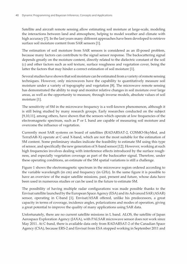
Figure 1 shows the electromagnetic spectrum in the microwave region ordered according tothe variable wavelength (in cm) and frequency (in GHz). In the same figure it is possible tohave an overview of the major satellite missions, past, present and future, whose data havebeen used in numerous studies or can be used in the future to estimate SM.

The possibility of having multiple radar configurations was made possible thanks to theEnvisat satellite launched by the European Space Agency (ESA) and its Advanced SAR (ASAR)sensor, operating in C-band [1]. Envisat/ASAR offered, unlike his predecessors, a greatcapacity in terms of coverage, incidence angles, polarizations and modes of operation, givinga great potential to improve the quality of many applications using SAR data.

Unfortunately, there are no current satellite missions in L band. ALOS, the satellite of JapanAerospace Exploration Agency (JAXA), with PALSAR microwave sensor does not work sinceMay 2011. At C-band, there is available data only from RADARSAT-2 of the Canadian SpaceAgency (CSA), because ERS-2 and Envisat from ESA stopped working in September 2011 and

Dynamic Programming and Bayesian Inference, Concepts and Applications40

April 2012, respectively. For the future nearby, there are expected data from planned L-bandmissions, such as Argentinian 1A and 1B SAOCOM, whose first launch is expected between2014-2015; ALOS-2, which is expected to be launched in 2014. Also the SMAP active/passivesatellite from the National Aeronautics and Space Administration (NASA), expected for end2015, is very promising. SMAP will use high-resolution radar observations to disaggregatecoarse resolution radiometer observations to produce SM products at 3 km resolution. The SMhas been retrieved from radiometer data successfully using various sensors and platforms andthese retrieval algorithms have an established heritage [7].

The most valuable information for the study of the SM has been obtained through the combi‐nation of different frequencies, polarizations and angles of incidence, as demonstrated in [11,13,14,15]. The backscatter coefficient is highly sensitive to the micro roughness of the surfaceand vegetation coverage. These studies have been developed to determine the configurationof "optimal" sensor parameters, in terms of wavelength, frequency, polarization and angle ofincidence to reduce interference of these factors when making an accurate estimate of SM.

In reference to specific studies, Holah et al. (2005) [16] found that an accurate estimate of SMcan be achieved by using low or moderate (between 20° and 37°) incidence angles. Regardingpolarizations, the most sensitive to SM are found to be HH and HV polarization while the lesssensitive is VV. Li et al. (2004) [17] and Zhang et al. (2008) [18] found similar results. Further‐more Autret et al. (1989) [19] and Chen et al. (1995) [20] reported that the influence of surfaceroughness can be minimized by using co-polarized waves (HH/VV). Therefore, using multiple

Figure 1. Main satellite missions (past, recent and future) designed in the microwave region of the electromagneticspectrum (based on Richards, 2009).

Integration of Remotely Sensed Images and Electromagnetic Models into a Bayesian Approach for…http://dx.doi.org/10.5772/57562

41

polarizations should, in theory, improve the SM estimate. The general consensus of theliterature indicates that low incidence angles, long wavelengths (such as L-band) and both HHand HV polarization settings are the most appropriate sensor for an accurate SM estimate [1].

Another effective approach to mitigate the ambiguity introduced by the vegetation androughness is to focus attention on the temporal variations through time series of radar images.In this case the basis is to assume that the average roughness characteristics and vegetationremain almost unaltered while variations in moisture content affect backscatter signal alongthe time [21, 22]. In this regard, methods have been developed using change detection series,as in the recent study [23] Hornacek et al. (2012) used data from the wide swath Envisat/ASARacquisition mode as part of an evaluation of the potential of algorithms for estimating SM forSentinel-1 mission of ESA.

In remote sensing, researchers have to deal with two problems: the direct problem and theinverse problem. The direct problem refers to the development of electromagnetic models thatcan correctly characterize ground backscatter coefficient by using as input the sensor param‐eters, such as the angle of incidence (θi), the wavelength (λ) and a specified polarizationconfiguration, as well as soil parameters, such as dielectric constant and roughness.

These models provide a solid physical description of the interactions between the electromag‐netic waves and the objects on the Earth's surface (e.g., bare soil or vegetation), allowing tosimulate numerous experimental settings in terms of sensor configurations and soil charac‐teristics. The generality of models is a property essential to avoid dependence on local siteconditions and characteristics of the sensor, a situation that often occurs when working withevidence-based algorithms.

Once the models have been validated, it is possible to develop algorithms to invert thesemodels and predict soil surface properties using radar observations as inputs, which is thesolution to the inverse problem [24,25,26].

Numerous backscattering models have been developed in recent decades to help determinethe relationship between the measured signal at the sensor and biophysical parameters, withparticular emphasis on understanding the effects of surface roughness [11, 25, 27]. Consideringthe inversion of the direct models many approaches have been developed through numericalsimulations of forward models which include Look Up Tables, Neural Networks, Bayesianapproaches, and minimization techniques.

For example, the potential of some of these approaches to provide accurate maps of SM hasbeen investigated by Pampaloni et al. (2004) [28]. They conducted a performance comparisonof the three inversion algorithms using time series of Envisat ASAR cross-and co-polarizedimages on a farm site in Italy. The algorithms evaluated for accuracy, error rate and compu‐tational complexity were: multilayer perceptron neural network, a statistical approach basedon the Bayesian theorem and iterative optimization algorithm based on the Nelder-Meadmethod.

Among the different methods, the Bayesian approach has been deeply investigated for itscapability to provide an evaluation of the uncertainties on the variable estimates as well as thepossibility to create hierarchical models with different sources of information [11, 21, 29, 30].


The objective of this research is to examine the capability and accuracy of a Bayesian approachto retrieve surface SM setting different roughness and vegetation conditions in view of anoperational use of the algorithm. Several implementations of the main algorithm weredesigned to evaluate their different capabilities to reproduce the ground reference data. Inmost cases, these approaches are based on the assumption of predefined behavior of someparameters, such as vegetation and roughness, measured in situ, and then used as conditionalprobabilities.

The developed method has been applied to two main test sites, one located in Argentina andthe second in Iowa and exploited during the SMEX´02 campaigns. The comparison over twotest sites is useful to have confirmation on the behavior of the developed algorithms.

The SMEX’02 test site was one of the first exploited to test the proposed methodology that waslater extended to the Argentina test site.

For this reason larger space is given in this chapter to the Argentinean test site, where SM isbeing deeply studied because of the near future launch of the first SAOCOM satellite. In fact,there is a particular demand of SM maps from agricultural farmers of the Pampa region formonitoring the crop status, possible evaluation of water demand and yield assessment.

2. Remote sensing data and study areas

The proposed analysis is applied to two main datasets. The first dataset derives from anexperiment carried out in Argentina in view of the SAOCOM mission. The second one islocated in the USA and acquired during the SMEX’02 experiments where contemporary toSAR acquisitions intensively field campaigns were carried out.

2.1. Argentinean study area

The procedure adopted here was applied to data from SARAT L Band active sensor. TheSARAT SAR is an airborne sensor (figure 2) used to simulate the SAOCOM images to beanalyzed in feasibility studies. The SAR Airborne instrument works in L band (λ=23cm) andis fully polarimetric.

The data set consists of field soil moisture content measurements with the correspondingbackscattering coefficients at HH, HV, VH and VV polarizations and 25° incidence angleacquired with a L-band SARAT sensor. SARAT project includes an airborne sensor and anexperimental agricultural site. It is part of the SAOCOM mission of Argentinean Space Agency(CONAE). The main aim of the SARAT project is to provide full polarimetric SAR images todevelop and validate different applications before the launch of the first satellite SAOCOM,the SAOCOM 1A, estimated for the year 2014. The SAR instrument is installed on a BeechcraftSuper King Air B-200 from the Fueza Aérea Argentina (FAA) which has a nominal range offlight altitudes between 4000 and 6000 meters above the Earth's surface, resulting in theformation of images with angles of incidence between 20° and 70°.


43

Figure 2. SARAT instrument and Aircraft of the FAA.

This SAR system has the same characteristics of the upcoming SAOCOM. These characteristicsare described on Table 1.

Central frequency 1.3 GHz (L band)

Chirp bandwidth 39.8 MHz

Pulse duration 10 μm

Pulse Repetition Frequency 250 Hz

Swath 9 km (nominal to 4200 m of height)

Azimuth resolution 1.2 m (nominal)

Slant Range resolution 5.5 m

Spatial resolution 6 m (nominal)

Polarization Quad-Pol (HH, HV, VH y VV)

Incidence angle 20° - 70° (nominal to 4200 m of height)

Dynamic Range 45 dB

PSLR -25 dB

Noise equivalent σ0 -36.9 dB

Table 1. Technical characteristics of the SARAT sensor.

SARAT project also includes a validation sites in agricultural areas. For this study, an areainside the CETT (Teófilo Tabanera Space Center of CONAE) located in Cordoba province,


Argentina, was selected. Its central geographic coordinates are 31°31'15.08''S-64°27'16.32''W.Figure 3 shows the location of the test site.

Figure 3. Location of the test site at Conae, in Argentina.

The experimental site, chosen for SM, vegetation and surface roughness measurements, has10 fields with dimension of 50 m x 120 m which contain different kinds of crop and bare soil,as depicted in Fig. 4. All fields were intensively sampled during the SARAT acquisitions.

Plots with crops contain soybean, sunflower, corn and wheat crops. Figure 5 depicts cropsstage at the moment of the SARAT acquisition time.

Some plots were left without vegetation to better investigate the interaction of microwavesignal with roughness surfaces. The bare soil plots (1N, 2N, 1S and 2S) were ploughed withtwo roughness levels (low and high roughness) to evaluate the roughness impact on soilmoisture retrieval at plot level, as shown in Fig. 6.

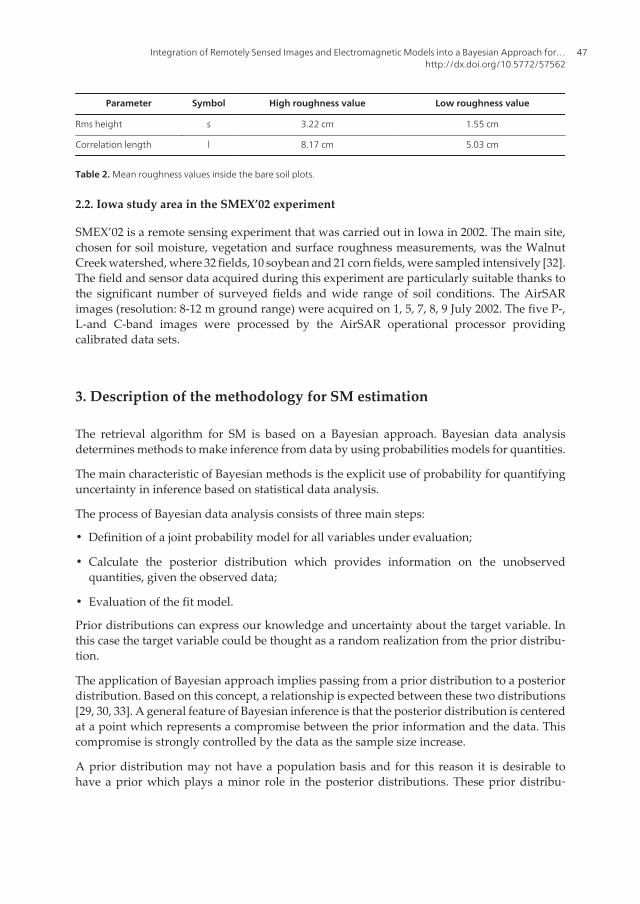
The roughness parameters, namely standard deviation of heights, s, and correlation length, l,were calculated as indicated in [31]. These parameters are listed in Table 2.

The SARAT images for this study (resolution: 9 m ground range) were acquired on February2012 and all the data was provided by CONAE. Soil moisture varied between 4% and 40%,even though most plots showed medium-dry conditions.


45

Figure 4. Detail of the sampled plots during SARAT campaign acquisitions. N and S indicate North and South testfields.

Figure 5. Soybeans, wheat (winter development), corn and sunflower.

Figure 6. Bare plot with induced low (left) and high roughness (right).


Parameter Symbol High roughness value Low roughness value

Rms height s 3.22 cm 1.55 cm

Correlation length l 8.17 cm 5.03 cm

Table 2. Mean roughness values inside the bare soil plots.

2.2. Iowa study area in the SMEX’02 experiment

SMEX’02 is a remote sensing experiment that was carried out in Iowa in 2002. The main site,chosen for soil moisture, vegetation and surface roughness measurements, was the WalnutCreek watershed, where 32 fields, 10 soybean and 21 corn fields, were sampled intensively [32].The field and sensor data acquired during this experiment are particularly suitable thanks tothe significant number of surveyed fields and wide range of soil conditions. The AirSARimages (resolution: 8-12 m ground range) were acquired on 1, 5, 7, 8, 9 July 2002. The five P-,L-and C-band images were processed by the AirSAR operational processor providingcalibrated data sets.

3. Description of the methodology for SM estimation

The retrieval algorithm for SM is based on a Bayesian approach. Bayesian data analysisdetermines methods to make inference from data by using probabilities models for quantities.

The main characteristic of Bayesian methods is the explicit use of probability for quantifyinguncertainty in inference based on statistical data analysis.

The process of Bayesian data analysis consists of three main steps:

• Definition of a joint probability model for all variables under evaluation;

• Calculate the posterior distribution which provides information on the unobservedquantities, given the observed data;

• Evaluation of the fit model.

Prior distributions can express our knowledge and uncertainty about the target variable. Inthis case the target variable could be thought as a random realization from the prior distribu‐tion.

The application of Bayesian approach implies passing from a prior distribution to a posteriordistribution. Based on this concept, a relationship is expected between these two distributions[29, 30, 33]. A general feature of Bayesian inference is that the posterior distribution is centeredat a point which represents a compromise between the prior information and the data. Thiscompromise is strongly controlled by the data as the sample size increase.

A prior distribution may not have a population basis and for this reason it is desirable tohave a prior which plays a minor role in the posterior distributions. These prior distribu‐


47

tions are considered as flat, diffuse or non-informative. The rational to use such types ofdistributions is to let the inference being not affected by external information and basedexclusively on data [34].

The proposed Bayesian approach is driven by both experimental data and theoretical electro‐magnetic models. The theoretical electromagnetic model has the main aim to simulate thesensor response by considering the characteristics of the soil and vegetation surface.

In order to have a better understanding of the proposed methodology, described in section3.2, a brief description of the electromagnetic models is presented in the next section.

3.1. Electromagnetic modeling

The development of physical or theoretical models simulating direct backscatter coefficientsin terms of soil attributes as dielectric constant and the surface roughness for an area of knowncharacteristics is one of the most common approaches for SM estimation (Barrett et al., 2009).Electromagnetic models allow a direct relationship between the surface parameters and thebackscattered radiation and are useful for understanding the sensitivity of the radar responseto changes in these biophysical variables.

Despite its complexity, only theoretical models can produce a meaningful understanding ofthe interaction between electromagnetic waves and the Earth's surface. However, exactsolutions of the equations that govern the rough surface scattering are not yet available andvarious approach methods have been developed with different ranges of validity [10]. Thestandard backscatter models are known as Kirchhoff Approximation (KA), which includes theGeometrical Optics Model (GOM), the Physical Optics Model (POM) and the Small Perturba‐tion Model (SPM). These models can be applied to specific conditions of roughness in relationto the sensor wavelength. For example, GOM is considered for very rough surfaces, POMmiddle roughness surfaces and SPM smooth surfaces.

The Integral Equation Model (IEM), based on the radiative transfer model, has beendeveloped by Fung and Chen in 1992 [27]. The model unifies the KA and the SPM model,a condition that makes it applicable to a wide range of roughness conditions. The IEMrequires, as inputs, sensor parameters such as polarization, frequency and incidence angle,and target parameters such as the real part of the dielectric constant, the RMS height, s,and the correlation length, l [27].

For the IEM model, the like polarized backscattering coefficients for surfaces are expressed bythis formula:

20 2 2

1

( 2k ,0)exp( 2k ) ,

2

(n)n x

pp z ppk=

Wkσ = s In!

¥ -- å (1)

where k is the wave number, θ is the incidence angle, kz=kcosθ, kx=ksenθ and pp refers to thehorizontal (HH) or vertical (VV) polarization state and s is the standard deviation of terrain


heights. The term I ppn depends on these parameters, k, s and on RH, RV, the Fresnel reflection

coefficients in horizontal and vertical polarizations. The Fresnel coefficients are strictlyrelated to the incidence angle and the dielectric constant. The symbol W (-2kx,0) is the Fouriertransform of the nth power of the surface correlation coefficient. For this analysis, anexponential correlation function has been adopted that seems to better describe theproperties of natural surfaces [27].

For vegetated soils, the simple approach, based on the so-called Water Cloud Model (WCM),developed by [35] has been considered in this analysis. In this radiative transfer model, thevegetation canopy as a uniform cloud whose spherical droplets are held in place structurallyby dry matter. The WCM represents the power backscattered by the whole canopy σ0 as theincoherent sum of the contribution of the vegetation σ0

veg and the contribution of the under‐lying soil σ0

soil, which is attenuated by the vegetation layer through the vegetation transmis‐sivity parameters τ2. For a given incidence angle the backscatter coefficient is represented bythe following expression:

0 0 2 0 .veg soilσ = σ σt+ (2)

If the terms related to vegetation and incidence angle are explicitly written in more detailedway, the backscattering coefficients become:

0 0cos (1 exp( 2 / cos )) exp( 2 / cos ),Esoilσ = A VWC B VWC σ B VWCq q q× × - - × × + × - × × (3)

where VWC is the vegetation water content (kg/m2), θ the incidence angle, σ0soil represents the

backscattering coefficient of bare soil that in this case calculated by using the IEM model, τ2 isthe two-way vegetation transmissivity with τ2=exp(-2B VWC/ cosθ). The parameters A, B andE depend on the canopy type and require an initial calibration phase where they have to befound in dependence of the canopy type and with the use of ground data.

In this work the model simulation enters directly in the inversion procedure. For the Bayesianapproach, the simulated data are generated in order to compare them to the measured dataand to create the noise probability density function (PDF) as detailed in the section devoted tothis approach. For this reason, it is needed to perform a preliminary validation of the proposedmodel as their simulation enters directly the inversion procedure.

Calibration constant values of the WCM, namely A, B and E were taken initially from literatureto take into account the effect of vegetation on the SAR signal [36]. Subsequently through aMaximum Likelihood approach they were determined to fit the data used in this work fromboth test sites. The application of calibration equations considers two different kind ofvegetation, with respect to the sensor response: very dense vegetation (as corn and sunflower)and less dense vegetation (soybean and grass). This step includes the NDVI calculation fromsome SPOT and LANDSAT optical images for the Argentinean and SMEX’02 test site respec‐


49

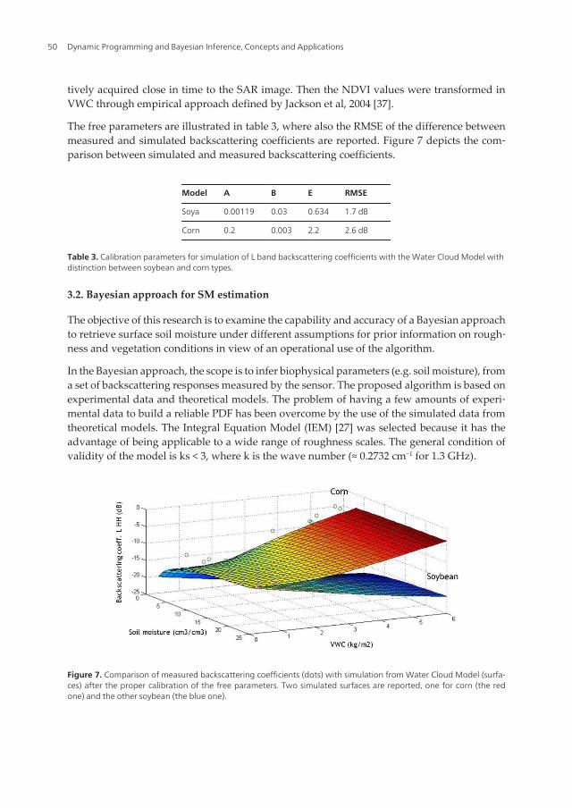
tively acquired close in time to the SAR image. Then the NDVI values were transformed inVWC through empirical approach defined by Jackson et al, 2004 [37].

The free parameters are illustrated in table 3, where also the RMSE of the difference betweenmeasured and simulated backscattering coefficients are reported. Figure 7 depicts the com‐parison between simulated and measured backscattering coefficients.

Model A B E RMSE

Soya 0.00119 0.03 0.634 1.7 dB

Corn 0.2 0.003 2.2 2.6 dB

Table 3. Calibration parameters for simulation of L band backscattering coefficients with the Water Cloud Model withdistinction between soybean and corn types.

3.2. Bayesian approach for SM estimation

The objective of this research is to examine the capability and accuracy of a Bayesian approachto retrieve surface soil moisture under different assumptions for prior information on rough‐ness and vegetation conditions in view of an operational use of the algorithm.

In the Bayesian approach, the scope is to infer biophysical parameters (e.g. soil moisture), froma set of backscattering responses measured by the sensor. The proposed algorithm is based onexperimental data and theoretical models. The problem of having a few amounts of experi‐mental data to build a reliable PDF has been overcome by the use of the simulated data fromtheoretical models. The Integral Equation Model (IEM) [27] was selected because it has theadvantage of being applicable to a wide range of roughness scales. The general condition ofvalidity of the model is ks < 3, where k is the wave number (≈ 0.2732 cm−1 for 1.3 GHz).

Figure 7. Comparison of measured backscattering coefficients (dots) with simulation from Water Cloud Model (surfa‐ces) after the proper calibration of the free parameters. Two simulated surfaces are reported, one for corn (the redone) and the other soybean (the blue one).


For bare soil, these unknown parameters are the real part of the dielectric constant (ε), thestandard deviation of the height (s) and the correlation length (l), the latter two describing themorphology of the surface. For vegetated fields, the Bayesian inversion was performed undertwo different approaches. In one case the Water Cloud Model (WCM) [35] is used to simulatethe backscattering coefficients from vegetation. In the second case, the PDF parameters areproperly modified to take into account vegetation effect through empirical relation withvegetation [38]. In both cases, the Vegetation Water Content (VWC) is added as unknownparameter, and it is derived from optical images. In this way, the approach exploits a synergybetween SAR and optical images.

At the beginning, the conditional probability is assumed as normal distribution. In the trainingphase, the conditional PDF is evaluated using measured data (fim) and simulated values fromthe IEM model (fith). The distribution assumption is then verified with a chi-squared statistics.The noise function Nl (eq. 4) and the related PDF parameters (mean and standard deviation)are calculated from the statistics of the ration between measured and simulated backscatteringcoefficients as follows [11, 39]:

.imi

ith

fN

f= (4)

Subsequently a joint PDF is obtained as a convolution of single independent PDFs. The jointPDF is a posterior probability derived from prior probability on roughness and soil moisturevalues and to the conditional probability which relates the variations of backscatteringcoefficients to variations of soil moisture and roughness. The relationship can be expressed asfollows:

( ) ( ) ( )( ) ( )

00

0,prior i post i i

i iprior i post i i i

Si

p S p Sp S

p S p S dS

ss

s=ò (5)

where the term at the denominator is a normalization factor with integration over all variablesSi. The variables Si can be:

• For bare soil: dielectric constant (ε), the standard deviation of the height (s) and the corre‐lation length (l);

• For vegetated soil: dielectric constant (ε), the standard deviation of the height (s) and thecorrelation length (l), vegetation water content (VWC).

The variables σ0i refer to the input values derived from remote sensing data, which in the

presented approach are:

• Backscattering coefficients at L-band HH and VV pol for the Argentinean test sites;


51

• Backscattering coefficients at C-band HH and VV pol, L-band HH and VV pol and thecombination of C and L band at HH pol for SMEX’02 test site.

Based on the field data, the integration ranges for Bayesian inference were selected withdifferent values as is illustrated in the following part. The main aim of using different intervalswas to test the sensitivity of the methods to prior information, Through these integrations, toeach pixel a value of dielectric constant is associated, starting from the corresponding back‐scattering coefficient values. Finally, with the formula proposed by [40] the dielectric constantvalues have been transformed to estimated values of soil moisture. The flowchart in Fig.8outlines the main steps of the algorithm, including training and test phase.

Figure 8. Flowchart of the Bayesian soil moisture approach applied to the Argentinean test site.

As above mentioned, another version of the Bayesian algorithm was developed to take intoaccount the effect of vegetation into the PDF. The flowchart of the algorithm is the same asshown in fig.8, but instead of Water Cloud Model there is an adaptation of the PDF mean toan empirical function related to VWC as detailed described in Notarnicola et al., 2007 [38]. Thealgorithm was developed to work with C, L and combination of C and L band. In this work,this specific algorithm is applied to SMEX’02 data.


4. Results and discussion

The main aim of the work is to verify the sensitivity of the algorithm to prior conditions ofroughness and vegetation in order to optimize the accuracy of the results. Based on this conceptseveral retrievals were performed for different conditions of surface roughness, with specificalgorithms for each coverage type in the study area. In the following the results on theArgentinean and SMEX’02 test sites are presented and discussed.

4.1. Argentinean test site

Over the Argentinean test site, the algorithm (fig.8) is divided in two main parts: one to beused in plots with bare soil or covered with sparse vegetation and another for vegetated soils.In both cases, two versions of the algorithm were developed: a simplified one working on avector of mean values for each plot where the aim is to analyze the backscatter coefficientbehavior using random values within ranges of s and l, and another one to work on the wholeimage, on pixel basis, to investigate the SM spatial distributions. Working with average valuesof backscattering coefficients has two objectives: to understand the effect on the SM estimateswhen the signal noise in the single plot is strongly reduced and to lower the computationburden when applying a random function for s and l variables.

An extensive analysis was conducted in order to understand the behavior of variables such assurface roughness and vegetation presence in the final SM estimation through the variabilityof the prior information. The different cases analyzed are listed below:

• Case 1: Pixel based algorithm for bare soil with fixed roughness. Three runs were executed:s=0.3 cm, l=5.0 cm; s=0.5 cm, l=5.0 cm and s=0.9 cm, l=5.0 cm. Then a mean value map isgenerated.

• Case 2: Pixel based algorithm for bare soil with an integration over a roughness range: 0.6cm < s < 1.4 cm; l=5.0 cm.

• Case 3: Pixel based algorithm for bare soil with an integration over a roughness range: 0.6cm < s < 1.4 cm; l=15.0 cm.

• Case 4: Pixel based algorithm for bare soil with an integration over a roughness range: 1.0cm< s < 1.5 cm; l=5.0 cm. In this case a very small integration range was considered.

• Case 5: Algorithm applied to backscattering coefficients averaged at plot level with arandom function. Values range: 0.5 cm < s < 1.2 cm; 5.0 cm < l < 10.0 cm.

• Case 6: VWC is calculated using a SPOT image. Fixed roughness and correlation length.s=0.5 cm; l=5.0 cm.

• Case 7: VWC is calculated using a SPOT image and a random function is implemented fors and l calculation, considering expected mean and standard deviation values for eachparameter: mean value of s=0.7 cm and standard deviation value of 0.5 cm, mean value ofl=5.0 cm and standard deviation of 5.0 cm. The random function is built as a noise function


53

added to the mean values of s and l. The pseudo random values are drawn from a standardnormal distribution.

• Case 8: VWC is provided as an input variable and an integration is done over the followingvalues: 0.01 <VWC < 6 Kg m2.

• Case 9: VWC is calculated using a SPOT image, based on NDVI values, and an integrationis done over roughness and correlation length in the following ranges:0.4 cm< s < 1.2 cm and3.0 cm < l < 10.0 cm.

In Fig.9, preliminary results are presented where the different analyzed cases based on variousprior conditions are numbered from 1 to 9. In general, for bare soil (fig. 9), the results showeda sensitivity of the algorithms to the different roughness conditions of each plot with avariability of around 5-7% (excluding the extreme cases). The highest variability among thecases is around 40% and is found when the roughness interval is very small (case 2 and 3).When considering a random function for roughness (case 7) and when performing the retrievalover average values of backscattering coefficients (case 5), the mean different with respect toground measurements is around 15%.

For vegetated areas, due to the limited availability of field measurements (field 5N), theevaluation of the performances is still under work. More extensive results for vegetation arepresented for the SMEX’02 experiments.

Figure 9. Comparison of SM estimates with measured values. Behavior diagram of the described cases.


Case1 and 3 results are reported in the form of SM maps in fig.10. A detailed analysis of themaps in fig.10 indicated error patterns detected for cases with rows of plots oriented orthog‐onally to the direction of the sensor observation. As it was observed, the backscatteringcoefficients for HH polarization is sensitive to the orientation of lines tillage and no inversionalgorithms consider this factor. Consequently the results show significant errors in plotsperpendicular to the observation.

Figure 10. Soil moisture maps for Case 1 (left) and Case 3 (right) over the selected test site.

Case 1 shows that the northern plots with bare soils (1N and 2N) have moisture values verysimilar to the ground truth. On the contrary, southern plots with bare soils (1S and 2S) havehigher moisture values than the measured ones, having the first of them a value of 25%, whilethe in situ data shown values around 20%. Case 3 shows that plot 1N and 2N obtained moisturevalues around 15%, which represents an over-estimation of the actual value of around 5%. Forplots 1S and 2S, the estimate values are between 22 to 24%. Case 1 could model with goodaccuracy plots 1N and 2N losing accuracy in southern plots. On the contrary, Case 3 couldmodel with relatively accuracy plots 1S and 2S losing precision in northern plots. The factorof apparent roughness change can be attributed to the orientation of the rows with respect tothe SAR signal [41].

4.2. Results on the SMEX’02 experiments

As illustrated in previous paragraphs, the inversion methodologies based on Bayesianapproach can be applied to different sensors configurations. In this way different polarizationsand/or bands can be exploited to extract soil features. In fact, due to the different way C bandor L band signals interact with soil and the above canopy layer, they are sensitive to differentsurface characteristics. Thus a proper combination of the two bands can help disentangle the


55

effect of vegetation and then improve the estimation of soil moisture. In this paragraph, theresults of the Bayesian methodologies are illustrated and the evaluated in terms of:

• Correlation coefficients, R, between the estimates and the ground truth values

• Root Mean Square Error, RMSE, between the estimates and the ground truth values.

When dealing with the different cases due to the prior information, the retrieved values willbe compared with the measurements through the Taylor plots [42].

The Bayesian approach has been applied to AirSAR data collected during the SMEX’02experiments considering C band, L band and combination of C and L data.

The results for the estimation of SM are reported in table 4. As expected the estimation of SMis quite difficult, thus determining values of R varying from 0.47 to 0.80 for the combinationof C and L bands. The highest difficulties are found for the detection and correct estimation ofextreme values of soil moisture.

Configurations Correlation coefficients RMSE (cm3/cm3)

C band 0.47 0.10

L band 0.67 0.05

C + L band 0.80 0.02

Table 4. Correlation coefficients (R), RMSE for the comparison between the different estimates and ground truthvalues for SM values, excluding extreme values.

The retrieval of low values of SM can be difficult as the signal for soil is small and difficult tobe disentangled from the vegetation signal. For high values, the signal from soil is strong butin the case of C bands the double bouncing and the effect of absorption from leaves also for Lband, typical of narrow leaf plants such as soybean, determine a lower signal reaching thesensor [43]. The L band estimates are the only one able to predict highest values of SM.

Similar analyses were also found in Notarnicola et al. 2006 [39]. In this previous analysis, themethodologies were applied only to few fields of the same data set. With respect to the accuracyreported in Notarnicola et al., 2006 [39], a worsening in the performance is found. In particularthe data set includes all the fields in the watershed basin and the fields located in the easternpart which exhibits anomalous values of SM, some very high values around 35% and somevalues lower than 5%. Considering the available meteorological information, the eastern andwestern parts of the watershed experienced very different intensity for the rain event wheremost of the rain event occurred in the western part.

If the watershed is divided in two parts the western and the eastern part the performances ofthe algorithm for SM retrieval differ significantly. The correlation coefficients are equal to 0.57and 0.84, not significantly different from those found in [39].

Furthermore, the performances notably change if in the data set the soybean and corn fieldsare considered separately. The results are reported in table 5.


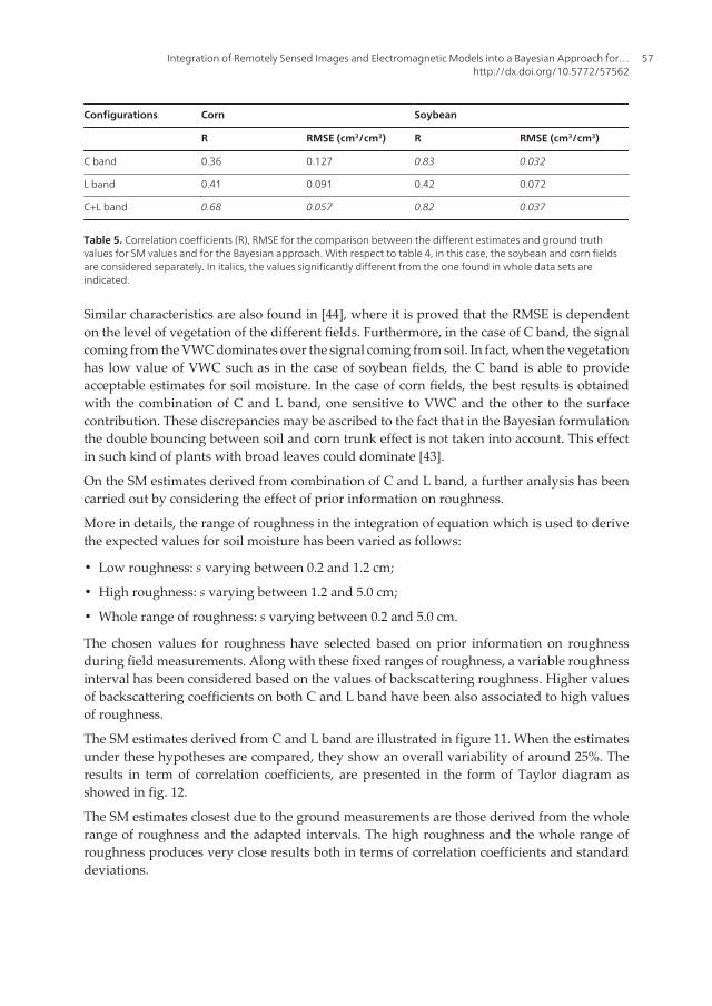
Configurations Corn Soybean

R RMSE (cm3/cm3) R RMSE (cm3/cm3)

C band 0.36 0.127 0.83 0.032

L band 0.41 0.091 0.42 0.072

C+L band 0.68 0.057 0.82 0.037

Table 5. Correlation coefficients (R), RMSE for the comparison between the different estimates and ground truthvalues for SM values and for the Bayesian approach. With respect to table 4, in this case, the soybean and corn fieldsare considered separately. In italics, the values significantly different from the one found in whole data sets areindicated.

Similar characteristics are also found in [44], where it is proved that the RMSE is dependenton the level of vegetation of the different fields. Furthermore, in the case of C band, the signalcoming from the VWC dominates over the signal coming from soil. In fact, when the vegetationhas low value of VWC such as in the case of soybean fields, the C band is able to provideacceptable estimates for soil moisture. In the case of corn fields, the best results is obtainedwith the combination of C and L band, one sensitive to VWC and the other to the surfacecontribution. These discrepancies may be ascribed to the fact that in the Bayesian formulationthe double bouncing between soil and corn trunk effect is not taken into account. This effectin such kind of plants with broad leaves could dominate [43].

On the SM estimates derived from combination of C and L band, a further analysis has beencarried out by considering the effect of prior information on roughness.

More in details, the range of roughness in the integration of equation which is used to derivethe expected values for soil moisture has been varied as follows:

• Low roughness: s varying between 0.2 and 1.2 cm;

• High roughness: s varying between 1.2 and 5.0 cm;

• Whole range of roughness: s varying between 0.2 and 5.0 cm.

The chosen values for roughness have selected based on prior information on roughnessduring field measurements. Along with these fixed ranges of roughness, a variable roughnessinterval has been considered based on the values of backscattering roughness. Higher valuesof backscattering coefficients on both C and L band have been also associated to high valuesof roughness.

The SM estimates derived from C and L band are illustrated in figure 11. When the estimatesunder these hypotheses are compared, they show an overall variability of around 25%. Theresults in term of correlation coefficients, are presented in the form of Taylor diagram asshowed in fig. 12.

The SM estimates closest due to the ground measurements are those derived from the wholerange of roughness and the adapted intervals. The high roughness and the whole range ofroughness produces very close results both in terms of correlation coefficients and standarddeviations.


57

Figure 11. Comparison of SM estimates under different roughness hypothesis with ground measurements. “LR” standfor low roughness, “HR” for high roughness, “Whole” for the whole range of roughness and adaptive for adaptivevalues of roughness.

Figure 12. Taylor diagram showing the comparison under different prior hypotheses on roughness. A refers toground measurements; B to low roughness; C to high roughness; D to whole range of roughness; E adapted rough‐ness ranges.


5. Conclusions

The main objective of this chapter is to present the capability of Bayesian approach to estimateSM values starting from SAR backscattering coefficients. Two case studies are presented whereSAR acquisitions took place over agricultural fields. The first case study was related to anArgentinean test site developed and equipped for acquisitions of airborne L band SAR calledSARAT. The acquisitions were carried out in preparation of the SAOCOM mission. The secondcase study was related to the experiment SMEX’02 carried out in IOWA in 2002. In thisexperiment airborne AirSAR images were available and for this reason the retrieval wasapplied to C band, L band and C+L band data.

Based on the retrieval results, the main goal was then to verify the sensitivity of the SMestimates from the set prior information on roughness and vegetation. All the prior PDFs areset a uniform, non-informative but the set limits of the interval in the integration procedurecan determine variation in the final SM estimates. This behavior is expected because theelectromagnetic models used in the retrieval approach contain explicitly the dependence ofbackscattering coefficients on roughness and vegetation parameters.

The effect of prior information ranges from few percentages up to 25% where the highestsensitivity is found in both case studies when too specific and narrow intervals for roughnessare used. The highest performances were found for both case studies when the range ofroughness is large enough to include most roughness measurements. Moreover, if a prelimi‐nary assessment on the roughness level is available, the algorithm determines the highestperformances with respect to the ground reference data.

An interesting feature observed in the case of Argentinean test site is the reduction of errorson the SM estimates when the retrieval is performed on average values of backscatteringcoefficients from each field. This behavior can be due to the reduction of noise present in theSAR signal.

As main conclusion of this analysis and suggestions in using the proposed the Bayesianalgorithms for SM estimation, the following considerations emerge:

• The set of prior information has to be selected carefully;

• Even in the case of non-information prior PDF, the range of variability of the prior variablehas an impact on the final estimates;

• It is preferable to integrate over a large interval of roughness and/or vegetation variables inorder to take into account and properly weight all the measured values.

• As the speckle noise can influence the SM estimates, a proper filter over the SAR imageneeds to be applied before proceeding to the retrieval approach.


59

Acknowledgements

The authors wish to thank to CONAE and SAOCOM mission team for SARAT data provisionand field measurements acquired during the remote sensing campaign.

Author details

Claudia Notarnicola1* and Romina Solorza2

*Address all correspondence to: [email protected]

1 EURAC Research-Institute for Applied Remote Sensing, Viale Druso, Bolzano, Italy

2 Gulich Institute, CONAE, Falda del Carmen, Córdoba, Argentina

References

[1] Barrett B.W., Dwyer E., Whelan P. Soil Moisture Retrieval from Active SpaceborneMicrowave Observations: An Evaluation of Current Techniques. Remote Sens., 2009;1 210-242, doi:10.3390/rs1030210.

[2] World Meteorological Observatory, Climate Essential Variable http://www.wmo.int/pages/prog/gcos/index.php?name=EssentialClimateVariables (access 5 November2013).

[3] Álvarez Mozos J., Casalí J., González A., López J. Estimación de la Humedad Superfi‐cial del Suelo mediante Teledetección de Radar en Presencia de una Cubierta de Ce‐real. Estudios de la Zona No Saturada del Suelo, 2005; VII 313–318.

[4] Engman E.T. Applications of microwave remote sensing of soil moisture for waterresources and agriculture. Remote Sensing of Environment, 1991; 35 213–226,.

[5] Ulaby F.T., Aslam A., Dobson M.C. Effects of vegetation cover on the radar sensivityto soil moisture. IEEE Transactions on Geoscience and Remote Sensing, 1982; 20(4)476–481.

[6] Lakshmi V. Remote Sensing of Soil Moisture. Hindawi Publishing Corporation ISRNSoil Science Volume 2013, Article ID 424178, 33 pages.

[7] Gruhier C., de Rosnay P., Hasenauer S., Holmes T., de Jeu R., Kerr Y., Mougin E.,Njoku E., Timouk F., Wagner W., Zribi M. Soil moisture active and passive micro‐wave products: intercomparison and evaluation over a Sahelian site, Hydrol. EarthSyst. Sci., 2010; 14 141–156.


[8] Behari J. Microwave Dielectric Behavior of Wet Soils. Anamaya Publishers, 2005.

[9] Ulaby F. T. Radar measurement of soil moisture content. IEEE Transactions on An‐tennas and Propagation, 1974; 22(2) 257–265. doi: 10.1109/TAP.1974.1140761.

[10] Ulaby F.T., Moore R.K., Fung A.K. Microwaves Remote Sensing: Active and Passive.,volume III, Surface Scattering and Emission Theory. Artech House, Dedham, MA,1986.

[11] Dubois P., Van Zyl J., Engman T. Measuring soil moisture with imaging radars. IEEETransactions on Geoscience and Remote Sensing, 1995; 33 (4) 915–926.

[12] Baghdadi N., Aubert M., Zribi M. Use of TerraSAR-X Data to Retrieve Soil MoistureOver Bare Soil Agricultural Fields. IEEE Geoscience and Remote Sensing Letters,2012; 9(3) 512–516.

[13] Dobson F.T. Ulaby L.E. Pierce, T.L. Sharik K.M. Bergen J. Kellindorfer J.R. Kendra E.Li Y.C. Lin A. Sarabandi K., Siqueira P.. Estimation of forest byophysical characteris‐tics in northern michigancwith sir-c/x-sar. IEEE Transactions on Geoscience and Re‐mote Sensing, 1995; 33 877–895.

[14] Ferrazzoli P., Paloscia S., Pampaloni P., Schiavon G. The potential of multifrequencypolarimetric sar in assesing agricultural and arboreous biomass. IEEE Transactionson Geoscience and Remote Sensing, 1997; 35 5–17.

[15] Baronti S., Del Frate F., Ferrazzoli P., Paloscia S., Pampaloni P., Schiavon G.. SAR po‐larimetric features of agricultural areas. International Journal of Remote Sensing,1995; 16 2639–2356.

[16] Holah N., Baghdadi N., Zribi M., Bruand A., King C.. Potential of ASAR/Envisat forthe characterization of soil surface parameters over bare agricultural fields. RemoteSensing of Environment, 2005; 96 78–86.

[17] Li Z., Ren X., Li X., Wang L. Soil moisture measurement and retrieval using EnvisatASAR imagery. Proceedings of the IEEE International Geoscience and Remote Sens‐ing Symposium (IGARSS 2004), 3539–3542, Anchorage, USA, 2004.

[18] Zhang T., Zeng Q., Li Y., Xiang Y. Study on relation between InSAR coherence andsoil moisture. Proceedings of the ISPRS Congress, Beijing, China, 2008.

[19] Autret, Bernard R., VidalMadjar D.. Theoretical study of the sensitivity of the micro‐wave backscattering coefficient to the soil surface parameters. International Journalof Remote Sensing, 1989; 10 171–179.

[20] Chen K.S., Yen S.K., Huang W.P.. A simple model for retrieving bare soil moisturefrom radar scattering coefficients. Remote Sensing of Environment, 1995; 54 121–126.

[21] Pierdicca N., Pulvirenti L., Bignami C.. Soil moisture estimation over vegetated ter‐rains using multitemporal remote sensing data. Remote Sensing of Environment,2010; 114 440–448.


61

[22] Balenzano A, Satalino G., Belmonte A., D’Urso G., Capodici F., Iacobellis V., Gioia A.,Rinaldi M., Ruggieri S., Mattia F. On the use of multitemporal series of COSMO-SkyMed data for LANDcover classification and surface parameter retrieval over agri‐cultural sites. Proceeding of Geoscience and Remote Sensing Symposium (IGARSS),142–145, July 2011.

[23] Hornacek M, Wagner W, Sabel D, Truong H.L, Snoeij P, Hahmann T, Diedrich E,Doubkova M. Potential for High Resolution Systematic Global Surface Soil MoistureRetrieval Via Change Detection Using Sentinel-1. IEEE Journal of Selected Topics inApplied Earth Observations and Remote Sensing, 2012, 1–9.

[24] Dobson M.C., Ulaby F. T.. Mapping Soil Moisture Distribution With Imaging Radar,chapter 8, 407–433. John Wiley and Sons Inc., 1998.

[25] Shi J., Wang J., Hsu A.Y., ONeill P.E., Engman E.T.. Estimation of bare surface soilmoisture and surface roughness parameter using l-band SAR image data. IEEETransactions on Geoscience and Remote Sensing, 1997; 35 1254–1266.

[26] Oh Y.. Quantitative retrieval of soil moisture content and surface roughness frommultipolarized radar observations of bare soils surfaces. IEEE Transactions on Geo‐science and Remote Sensing, 2004; 42(3) 596–601.

[27] Fung, A. K. Microwave Scattering and Emission Models and their Application. Ar‐tech House, Boston; 1994.

[28] Pampaloni P., Santi E., Paloscia S., Pettinato S., Poggi P. Radar Remote Sensing ofSoil Moisture, ENVISNOW Project, SMC algorithms. Technical report, IFAC-CNR,October 2004.

[29] Notarnicola C., Posa F. Bayesian algorithm for the estimation of the dielectric con‐stant from active and passive remotely sensed data. IEEE Geoscience and RemoteSensing Letters, 2004; 1(3) 179–183.

[30] Paloscia S., Pampaloni P., Pettinato S., Santi E. A comparison of algorithms for re‐trieving soil moisture from ENVISAT/ASAR images. IEEE Transactions on Geosci‐ence and Remote Sensing. 2008; 46(10) 3274-3284.

[31] Barber M., Grings F., Perna P., Bruscantini C., Karszenbaum H. Análisis de las medi‐ciones de rugosidad del Centro Espacial Teófilo Tabanera, Córdoba. Technical report,CONAE-IAFE,Mayo

[32] http://nsidc.org/data/amsr_validation/soil_moisture/smex02/

[33] Barber M., Grings F., Perna P., Piscitelli M., Maas M., Bruscantini C., Jacobo-Berlles J.,Karszenbaum H. Speckle Noise and Soil Heterogeneities as Error Sources in a Bayesi‐an Soil Moisture Retrieval Scheme for SAR Data. IEEE Journal Of Selected Topics InApplied Earth Observations And Remote Sensing, 2012; 5(3).


[34] Gelman A., Carlin J.B., Stern H.S., Rubin D. B., Bayesian data analysis, Chap‐man&Hall/CRC 1995.

[35] Attema E. P, Ulaby F.T.. Vegetation Modeled as a Water Cloud. Radio Science, 1978;13(2) 357–364.

[36] Dabrowska-Zielinska K., Inoue Y., Kowalik W., Gruszczynska M.. Inferring the effectof plant and soil variables on C-and L-band SAR backscatter over agricultural fields,based on model analysis. Advances in Space Research, 2007; 39 139–148.

[37] Jackson T., Chen D., Cosh M., Li F., Anderson M., Walthall C., Doriaswamy P., RayHunt E. Vegetation water content mapping using Landsat data derived normalizeddifference water index for corn and soybeans. Remote Sensing of Environment, 2004;92 475–482.

[38] Notarnicola, C. & Posa, F. Inferring vegetation water content from C and L band im‐ages, IEEE Transactions on Geoscience and Remote Sensing, 2007; 45(10) 3165-3171.

[39] Notarnicola C., Angiulli M., Posa F. Use of Radar and Optical Remotely Sensed Datafor Soil Moisture Retrieval on Vegetated Areas. IEEE Transactions on Geoscience andRemote Sensing, 2006; 44(4) 925-935.

[40] Hallikainen M.T., Ulaby F.T., Dobson M.C., El Rayes M.A., Wu L.K.. Microwave die‐lectric behavior of wet soil-part 1: Empirical models and experimental observations.IEEE Transactions On Geoscience And Remote Sensing, 1985; GE-23(1) 25–34.

[41] Solorza R., Notarnicola C., Karszenbaum H., Retrieval of soil moisture using a Baye‐sian approach and electromagnetic models in views of the SAOCOM mission: studyon SARAT images in an agricultural site in Argentina, Proceeding of Igarss 2013, July2013, Melbourne, Australia.

[42] Taylor, E, K, Summarizing multiple aspects of model performance in a single dia‐gram, Journal of Geophysical Research, 2001; 106(D7), 7183-7192.

[43] Macelloni G., Paloscia S., Pampaloni P., Marliani F., Gai, M. The relationship betweenthe backscattering coefficient and the biomass of narrow and broad leaf crops, IEEETransaction on Geoscience and Remote Sensing, 2001; 39(4) 873-884.

[44] Lakhankar T., Ghedira H., Temimi M., Sengupta M., Khanbilvar R., Blake, R. Non-parametric methods for soil moisture retrieval from satellite remote sensing data, Re‐mote Sensing, 2009; 1, 3-21. doi: 10.3390/rs1010003.


63

Documents

Integration of Remotely Sensed Images and …cdn.intechopen.com/pdfs/46452.pdf · Satellite and aircraft remote sensing allow estimating soil moisture at large-scale, modeling the