Embed Size (px)
Citation preview

IntegrationofOrbitalandGroundDataforMartianCraterMapping
AMethodologicalStudyatSantaMariaCrater
Thesis
Presented in Partial Fulfillment of the Requirements for the Degree Master of Science
in the Graduate School of The Ohio State University
By
Rui Wu, M.S.
Graduate Program in Civil Engineering
The Ohio State University
2012
Thesis Committee:
Rongxing Li, Advisor
Carolyn Merry
Alper Yilmaz

Copyright by
Rui Wu
2012

ii
Abstract
High-quality mapping products for Martian craters are helpful data sources for
scientists to explore the red planet in many fields. This thesis focuses on integrating
orbital imagery and ground imagery to generate high-quality Martian crater mapping
products. The usability of the proposed method is validated mainly at one crater –
Santa Maria Crater. The orbital imagery comes from the High Resolution Instrument
Scientific Experiment (HiRISE) camera onboard the Mars Reconnaissance Orbiter
(MRO) satellite. The ground imagery comes from the Navigation cameras (Navcams)
and Panoramic cameras (Pancams) images taken by the Opportunity rover in Mars
Exploration Rover (MER) mission.
In this thesis, important processes during the mapping will be introduced,
discussed, and analyzed, including interest point extraction, image network
construction, bundle adjustment (BA), dense matching, and product generation. Some
new methods during these processes are proposed to improve the quality of the final
products. The wide-baseline method is used in an unprecedented way in the tie point
selection to guarantee the accuracy of the distant tie points. An integrated bundle
adjustment replaces the former incremental bundle adjustment used in the MER
mission for large crater mapping. Matching in the featureless areas is also discussed in
this paper. The theoretical analysis and the improved results of these proposed
methods are highlighted with details.
The mapping products at Santa Maria Crater are listed to illustrate the feasibility

iii
of the proposed mapping methods.

iv
Dedication
To my parents –for giving me your eyes

v
Acknowledgements
Foremost, I want to thank my advisor, Dr. Rongxing Li, for leading me and
guiding me in the Master study and research. His thorough knowledge in the research
and endless enthusiasm for the job support and encourage me in this two-year
adventure. Without his guidance, I could never take the progress in the area of
photogrammetry and mapping, let alone writing this thesis to get the Master degree.
Besides my advisor, I would give my sincere thank to the rest of my thesis
committees: Dr. Carolyn Merry and Dr. Yilmaz, for their continuous encouragement
and advising.
My gratitude also goes to Dr. Kaichang Di, Dr. Shaoming Zhang, and Dr. Xuelian
Meng in the Mapping and GIS Lab, who helped me not only in the research with their
expertise, but also in my life with their rich experience.
I also want to thank my coworkers and friends in the Mapping and GIS Lab:
Liwen Lin, Wei Wang, Onur Karahayit, Ding Li, Shaojun He, I-Chee Lee, Jiangye
Yuan, Justin Crawford, Weishu Gong, and Leslie Smith, for the inspiring tutorials, for
the sleepless nights we worked together for the project, and for the laughter scattered
in every single day of the last two years.
And I want to express my deepest thank to my friend Min Wang. Her comfort is
the life saver for me when I feel hopelessness and desperation. I could not be the
current me without her encouragement.
Last but not least, I must thank my greatest parents. Their selfless support has
been, and will always be my source of spiritual strength.

vi
The research is supported by the Mars Data Analysis Program (MDAP) of
NASA.

vii
Vita
2004.......................................................Luhe First High School, Jiangsu, China
2008.......................................................B.S. GIS, Peking University, Beijing, China
2010.......................................................M.E. Photogrammetry and Remote Sensing,
Peking University, Beijing, China
2010 to present ......................................Graduate Research Associate, Department of
Civil Engineering, The Ohio State University
Publications Li, R., R. Wu, and X. Meng 2012. Wide-Baseline Mapping of Martian Craters: A
Comparison Study at Santa Maria Crater. ASPRS 2012 Annual Conference, 19-23
March, Sacramento, CA. Abstract no. 345409 (1 p.) and presentation.
Field of Study
Major Field: Civil Engineering

viii
TableofContentsAbstract .......................................................................................................................... ii
Dedication ..................................................................................................................... iv
Acknowledgements ........................................................................................................ v
Vita ............................................................................................................................... vii
List of Tables ................................................................................................................. ix
List of Figures ................................................................................................................ x
Chapter 1: Introduction .................................................................................................. 1
Chapter 2: Background of Orbital and Ground Data ..................................................... 8
Chapter 3: Construction of Image Network ................................................................. 22
Chapter 4: Integrated Bundle Adjustment .................................................................... 36
Chapter 5: Mapping Product Generation ..................................................................... 56
Chapter 6: Conclusions ................................................................................................ 70
References .................................................................................................................... 72

ix
ListofTables
Table 2-1. Important parameters of the camera system. ............................................ 11
Table 2-2. An example of RMC sequence. ................................................................17
Table 4-1. The statistics of the inconsistencies between features ..............................51
Table 4-2. The statistics of the consistency of features and rover positions ..............53
Table 5-1. The comparison on the dimension of Santa Maria Crater. .......................68

x
ListofFigures
Figure 1-1. The workflow of Martian crater mapping. ................................................6
Figure 2-1. HiRISE focal plane assembly layout. ........................................................9
Figure 2-2. Mars body-fixed reference system. .........................................................13
Figure 2-3. Landing site cartographic coordinate system. .........................................14
Figure 2-4. Site frame. ...............................................................................................15
Figure 2-5. Multiple instances of site frame. .............................................................16
Figure 2-6. Calculation of current position. ...............................................................20
Figure 3-1. Three types of tie points. .........................................................................23
Figure 3-2. Parallaxes of all candidate matching points and the parallax curve. .......26
Figure 3-3. The same feature observed from two different rover positions. .............27
Figure 3-4. Finding the feature correspondence by overlaying orthoimages. ...........28
Figure 3-5. The effect of baseline length on the accuracy .........................................30
Figure 3-6. The distribution of rover positions near ..................................................31
Figure 3-7. The result of rigid transformation when hard-baseline ...........................33
Figure 3-8. The construction of wide-baseline tie point selection. ............................34
Figure 3-9. The result of rigid transformation when wide-baseline ..........................34
Figure 4-1. Geometry of the collinearity. ...................................................................37
Figure 4-2. Typical landforms in Gusev Crater and Meridiani Planum. ....................43
Figure 4-3. The histograms of traverse in Gusev Crater and Meridiani Planum. ......44
Figure 4-4. Initialization of a rover position through feature comparison .................46
Figure 4-5. Shadows and shadings in HiRISE images of Martian craters. ................48

xi
Figure 4-6. The comparison between the DTMs generated from HiRISE images. ...49
Figure 4-7. Inconsistencies between features among multiple rover positions .........51
Figure 4-8. The consistency of rover positions and features between .......................53
Figure 5-1. “Rules” for choosing dense matching method. .......................................58
Figure 5-2. Geographe Crater with its blocked area. .................................................59
Figure 5-3. The dense matching points in Santa Maria Crater. ..................................61
Figure 5-4. Feature Comparison between the DTM of Santa Maria Crater ..............62
Figure 5-5. The detailed DTM at the sand dune area of Santa Maria Crater. ............63
Figure 5-6. The blocked areas in crater mapping. ......................................................64
Figure 5-7. Using the nearest pixels causes wrong filling in blocked areas. .............64
Figure 5-8. The brightness adjustment in sand dune area of Santa Maria Crater. .....66
Figure 5-9. Orthoimage of Santa Maria Crater before and after ................................66
Figure 5-10. Comparison between orthoimages generated via different methods. ...67
Figure 5-11. The product set at Santa Maria Crater. ..................................................69

1
Chapter1:Introduction
Mars, the nearest planet to the Earth, has been observed by human beings for
thousands of years. It is named after the Roman god of war, probably because its
passionate color seen from the Earth reminds people of wars. Nowadays, it attracts
more and more attention for the reason that it is still the only planet having the
possibility of life existence except for the Earth. Astronomers, geologists,
meteorologists, and biologists spend their lives on searching for evidence of life, or
the possibility of habitat on Mars. Telescopes, satellites, and rovers point to the Mars
trying to find any clue. Although no certain evidence has been found until now, people
don’t plan to stop their efforts.
Mars is the fourth planet in the solar system. It has the most similar environment
with the Earth. For example, its rotation period, also called solar day or sol, is 24
hours, 39 minutes, and 35.244 seconds (Allison and Schmunk, 2012), only a little
longer than an Earth day. And the surface of Mars is also covered with rocks, soil,
sand, which form different landforms such as craters, canals and mountains.
Meanwhile, there are also differences between the Mars and the Earth. For instance,
the atmosphere is much thinner than the one of the Earth and is composed mostly of
carbon dioxide (Coffey, 2008) instead of nitrogen and oxygen. But the difference that
matters most to the scientists is that no liquid water exists on Mars, which is the most
basic element to support life. This is also the reason that most life hunting missions
focus on looking for water instead of looking directly for life. As long as the evidence
of water exists now or in the past, it gives great opportunity to prove that there can be

1
life on Mars.
A regular way to find the evidence of water is to recognize the chemical
substances in rocks, sand, and soil, as well as to analyze the surrounding geologic
structure. Based on the experience on the Earth, certain chemical substances in certain
geologic structures are very strong indicators for fluvial processes. If similar
environment is found on Mars, it can be a solid evidence of water existence. Although
people have explored Mars for so many years, high-quality data for the
aforementioned method is still absent. No previous images or data can provide such a
resolution that the small rocks can be observed in detail, until the Mars Rover
Exploration (MER) mission and the High Resolution Instrument Experiment (HiRISE)
began (McEwen, et al., 2007).
Twin rovers, Spirit and Opportunity, were launched in the MER mission to
acquire close observation of Mars. They landed separately on Gusev Crater and
Meridiani Planum in 2004 and surprisingly survived after 90 sols of exploration as
planned, continuing their journey for over seven years so far. They have taken various
pictures of Mars with their camera systems. This system contains Navigation Cameras
(Navcam), Panoramic Cameras (Pancam), and Hazard Avoidance Cameras (Hazcam).
Navcam and Pancam can both provide high-resolution panorama images for Mars
surface mapping, which is essential for geologists to analyze the geologic structures
(Maki, et al., 2003). This thesis will focus on utilizing Navcam and Pancam images to
generate high-quality mapping products. On one hand, the ground images taken by
rovers are critical and quite useful. On the other hand, they cannot be used directly as
they are not processed at high level of mapping. This is not only about the image
quality itself, but also about the positioning information that records where those
images are taken precisely, and in what science context they are taken. The sandy

2
surface of Mars often causes slippage of the rover wheels, and then affects the
accuracy of the positioning information recorded by the rovers’ Inertial Measurement
Unit (IMU) (Ali, et al., 2005). Although the star tracking technique is also used for
rover positioning, the accuracy may be affected by the precision of timing. Therefore,
the attitudes of these images, or the rover localization, must be adjusted at first to
recover the correct positioning information when the images are taken. The most
popular and effective way to fulfill this image processing task is to construct the
image network using tie points among multiple rover positions, and then to bundle
adjust these positions to get consistency. This topic will be discussed in detail in
Chapter 3 and Chapter 4.
HiRISE is the camera onboard the Mars Reconnaissance Orbiter (MRO) satellite,
which was launched in 2005. It has 14 Charged-Coupled Devices (CCDs) working
together, providing high-resolution pictures of Mars surface in different spectrum
channels. By 2010, HiRISE has taken about 13000 images covering about 1% of Mars
(NASA, 2010) and the number keeps growing fast. The unprecedented spatial
resolution of the 0.25 m - 0.3 m imagery helps in discovering small interesting
features and landform patterns, such as Cape St. Vincent at Victoria Crater. Before
HiRISE, the highest resolution in satellite data is about 1.4 m in horizontal direction
(Malin, et al., 1992) by the Mars Orbiter Camera (MOC) narrow-angle and 1.5 m in
vertical direction by Mars Orbiter Laser Altimeter (MOLA) data (Zuber, et al., 1992).
Although MOLA data is still the best data that covers the whole Mars along and
across track, and can work as a reference in small scale, its horizontal resolution of
about 1 km (Zuber, et al., 1992) is too coarse for distinguishing small craters and
canals, let alone analyzing the attributes of rocks. Therefore, combining HiRISE
images and MOLA data is the most popular way to raise the usefulness of both

3
datasets. Hwangbo (2010) discussed this issue in detail. With the techniques in that
dissertation, HiRISE images controlled by MOLA data can provide very good Digital
Terrain Model (DTM) and orthoimage products for large area mapping at high quality.
It is easy to understand that ground images taken by rovers are proper for small
area mapping, such as craters, or canals, while orbital images taken by HiRISE are
proper for large areas, such as the planum, giant craters and mountains. Combining
the advantages of these two imaging data sets is promising to produce the best
mapping products for both levels. However, these two systems have very different
reference frames and imaging mechanisms, and the images are also taken in very
different angles of view, oblique in ground images and near-ortho in orbital images.
These problems make it difficult to combine them. To conquer the difficulties, the
first thing to do is to understand both imaging systems deeply and find the connection
between them. HiRISE images are taken from a satellite which is about 300 km above
Mars surface (Taylor, et al., 2006) without going through thick atmosphere, and then
controlled by MOLA data. It is reasonable to assume that they have a better global
geometric consistency, considering the blurring and the inaccuracy of distant features
seen commonly in ground images. Thus, HiRISE images controlled by MOLA data
can provide good initial positioning information, not only for rover positions, but also
for features from the ground images. This connection is used as a guideline in this
thesis and the practical analysis is elaborated in Chapter 4.
Since the accuracy of features, or tie points, are so important for recovering the
relationship among multiple rover positions, the whole Chapter 3 is dedicated to
introducing the method of selecting high-quality tie points, especially the usage of the
wide-baseline method in the process. Wide-baseline method has been used in so many
fields, especially photogrammetry and computer vision. The Mapping and GIS Lab in

4
The Ohio State University has also used this method for several crater mapping tests.
Those tests only utilized wide-baseline in the dense matching phase of DTM
generation, but never involved wide-baseline in the tie point selection phase. Chapter
3 will illustrate how the wide-baseline method can improve the quality of tie points
for bundle adjustment and how this improvement can affect the results.
With the tie points connecting all the ground images taken from multiple
positions, it is possible to adjust biased rover positions and get consistent results of
the 3D coordinates of those tie points via bundle adjustment, thus to recover the
precise positions. Previously, the Mapping and GIS Lab used incremental bundle
adjustment to guarantee the timeline required by the MER mission. It is in a step-wise
manner that only the latest position is considered as adjustable, which makes that only
two positions need to be considered every time. But error may be accumulated as the
traverse gets longer and longer. The integrated bundle adjustment proposed in this
thesis, on the contrary, performs bundle adjustment on multiple positions
simultaneously, so that the accumulated error in the whole image network within
these positions will be kept to a very low level. The theory of incremental and
integrated bundle adjustment and the comparison between them will be set forth in
Chapter 4.
Based on the results of bundle adjustment, all the features in the images should be
projected to a 3D model so that they can be observed in a simulated environment.
This process is done by dense matching and back-projection. Unlike the Earth full of
features in the environment, such as trees, buildings and other artificial features, Mars
is so desolated that the common features that can be used are rocks. In some sandy
areas in the Meridiani Planum, even rocks are so rare that the feature matching is far
from the standard definition of dense. Different matching methods need to be used to

5
automate this process, while onerous manual work is also inevitable to supplement the
result and ensure the matching quality. For Martian crater mapping, another common
issue is the blocked area matching. Wide-baseline, again, is known and tested to be
the best method to solve the problem. The content of dense matching and other
relevant methods will be discussed in Chapter 5.
These above steps are all necessary for a good-quality DTM and other related
mapping products. In order to evaluate these methods, mapping of Santa Maria Crater
in the landing site of Opportunity, the Meridiani Planum, is executed. Intermediate
data are illustrated to be analyzed, compared with previous methods, and final
products are compared to the HiRISE products to ensure the consistency. These tests
show that the proposed methods in this thesis are quite feasible for mapping most
small-to-medium scale Martian crater.
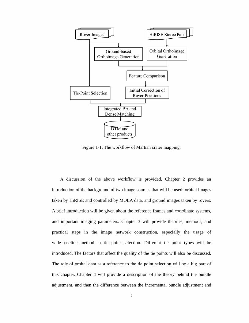
The workflow of Martian crater mapping can be seen in Figure 1-1.
6
Figure 1-1. The workflow of Martian crater mapping.
A discussion of the above workflow is provided. Chapter 2 provides an
introduction of the background of two image sources that will be used: orbital images
taken by HiRISE and controlled by MOLA data, and ground images taken by rovers.
A brief introduction will be given about the reference frames and coordinate systems,
and important imaging parameters. Chapter 3 will provide theories, methods, and
practical steps in the image network construction, especially the usage of
wide-baseline method in tie point selection. Different tie point types will be
introduced. The factors that affect the quality of the tie points will also be discussed.
The role of orbital data as a reference to the tie point selection will be a big part of
this chapter. Chapter 4 will provide a description of the theory behind the bundle
adjustment, and then the difference between the incremental bundle adjustment and

7
the integrated bundle adjustment. Their advantages and disadvantages will be put
forward so that they can be better used in different applications in the future. Chapter
5 is about the generation of the DTM and other mapping products. Dense matching
methods used in the tests will be introduced. The difficulty of complete autonomy in
matching will be emphasized. The principle behind back-projection is also explained.
Last but not least, the mapping results at Santa Maria Crater and other craters will be
given. Chapter 6 will provide a conclusion of the whole mapping process and discuss
the relevant future work.
8
Chapter2:BackgroundofOrbitalandGroundData
This chapter will provide an introduction of the information of the data sources
used in Martian crater mapping. The primary data source is the ground images taken
by the two rovers, Spirit and Opportunity, along their traverses in Gusev Crater and
Meridiani Planum over seven years. The second data source comes from the orbital
images taken by HiRISE onboard the MRO satellite controlled by MOLA data.
Necessary information about their imaging mechanisms and the reference frames will
be introduced.
2.1HighResolutionImagingScientificExperiment
HiRISE camera onboard the MRO satellite is designed to take very detailed
orbital images of Mars. This camera has 14 CCDs fixed to a focal plane, in which ten
are in red channel, two are in blue-green channel, and two are in the near infrared
(Figure 2-1). Rather than a frame imaging sensor, HiRISE takes images in a
pushbroom manner. Each CCD consists of 2048 pixels in the across-track direction
and 128 pixels in the along-track direction. In the across-track direction, the average
width of the overlap between adjacent CCDs is about 48 pixels. After aligning those
overlapping areas by adjustment, HiRISE can still have up to 20,264 pixels in the
across-track direction, which is equivalent to 6 km at 300 km altitude (Delamere et al.,
2003; McEwen et al., 2007).

9
Figure 2-1. HiRISE focal plane assembly layout (McEwen et al., 2010).
Two issues block the way to utilize HiRISE images for precise mapping. The first
one comes from the complexity of the sensor geometry among multiple CCDs.
Although they are all fixed to a focal plane and should produce consistent images with
each other, small systematic errors and certain random errors always bring in
unexpected distortion, bias, and offset. These disagreements among CCDs need to be
removed to achieve coherence in the exterior orientation parameters, and in the orbital
images.
The second issue is the inaccurate geopositioning of HiRISE images caused by no
ground truth. Unlike on the Earth, that various approaches can be used to measure the
ground control points for reference, the only measurements close to the ground truth
of Mars come from the MOLA data, which is still not dense enough. Without the

10
ground truth, the registration of HiRISE images can be largely affected by various
measurement errors.
A systematic approach has been developed by Hwangbo (2010) on solving these
issues by utilizing MOLA data and photogrammetry methods to register HiRISE
images. Since this is not the major topic of this thesis, the HiRISE images processed
by her method will be directly used here without detailed technical discussion.
2.2NavigationCamerasandPanoramicCameras
As twin sisters, Spirit and Opportunity have the same camera systems including
six engineering cameras and two science panoramic cameras. The primary goal for the
engineering cameras is to take necessary pictures for keeping the rover on track and
avoiding obstacles when doing blind drive, while the goal for the panoramic cameras
is to support high resolution imaging for scientific exploration of Mars.
The engineering cameras consist of two navigation cameras, two front Hazard
Avoidance Cameras (Hazcam) and two rear Hazcams. These four Hazcams are
mounted to the titanium alignment bracket under the solar panel with the baseline of
10 cm. They use visible light to capture images in black and white. The over 120
field of view (FOV) helps Hazcams to map out the shape of the terrain as far as 3 m in
front of the rovers, and the images work with built-in software to keep rovers from
crashing into unexpected obstacles (Maki, et al., 2003).
All mounted on the Panorama Mast Assembly (PMA), Navcams and Pancams are
good data sources for rover navigation, surface mapping and scientific research. The
PMA is capable of a rotation of 370 in the horizontal direction and a tilt of 194 in
the vertical direction, which makes it possible for Pancams and Navcams to take
panoramas of the surroundings. Because of the difference in the field of view, the
Navcams take a panorama using 10 stereo pairs, while the Pancams need 27 pairs.

11
The reliable distances of these two camera systems are also different as a result of
their configurations. Generally, Pancam is a better data source for mapping large
craters since the reliable distance is about 60 m, while Navcam is more appropriate
for mapping smaller craters within its 30 m reliable distance. More detailed
parameters of the camera systems onboard the twin rovers are listed in Table 2-1.
Camera Type Pancam Navcam Hazcam
FOV (Degree) 16*16 45*45 124*124
Baseline (cm) 30 20 10
Focal Length (mm) 43 14.67 5.58
Reliable Distance (m) 60 30 3
Angular Resolution (mrad/pixel) 0.28 0.82 2.1
Table 2-1. Important parameters of the camera system (Maki, et al., 2003).
The capability of the science panoramic cameras is reflected not only in the high
resolution, but also in the multispectral imaging filters. 13 filters are installed to take
images in different spectral bands, from near infrared to visible blue light. This is
essential for scientists when the characteristics of the materials on the Martian surface
can be learned based upon their spectral performances. However, for the purpose of
high-resolution crater mapping in this topic, a single spectral band is enough for us
during most of the time to distinguish different objects in the image for feature
extraction. According to the empirical experience, the red band (labeled as L2 and R2)
is used primarily in our experiments. When the red band is not available, the blue

12
band (labeled as L7 and R1) is used as an alternative (Bell III et al., 2004).
2.3MarsExplorationRoverCoordinateSystems
It is not difficult to understand that there are a number of reference frames and
coordinate systems for different applications in the MER mission. Understanding
these coordinate systems is the very first beginning to deal with the integration of
orbital data and the ground data. Considering the main topic of the thesis, this section
will only introduce the coordinate systems that are relevant to the Martian crater
mapping (Maki, 2003).
2.3.1MarsBody‐FixedReferenceFrame
The Mars body-fixed (MBF) reference frame is defined essentially by the
International Astronomical Union/International Association of Geodesy (IAU/IAG)
Working Group on Cartographic Coordinates and Rotational Elements of the Planets
and Satellites in their most recent report (Seidelmann et al., 2002). The Mars
body-fixed reference axes have their origin at the Mars center-of-mass and are aligned
with the spin axis and prime meridian. This frame is described as the following and
shown in Figure 2-2:
+XMBF=Vector lies in the Mars equatorial plane and intersects the prime meridian.
+YMBF=Vector lies in the Mars equatorial plane and completes a right handed
coordinate system.
+ZMBF =Mars spin axis, pointing toward Martian North Pole.

13
Figure 2-2. Mars body-fixed reference system.
2.3.2LandingSiteCartographicCoordinateSystem
More than one local reference system is defined for satellites and rovers for
various purposes. Among these reference systems the landing site cartographic (LSC)
coordinate system is particularly useful in navigation and imaging. The LSC
coordinate system is an East-North-Zenith (X-Y-Z) frame, whose origin is coincident
with the landing site, also called lander (Li, et al., 2004). Therefore, Spirit and
Opportunity both have their own LSC origins since the landers are located differently.
The LSC coordinate system is defined relative to the Mars body-fixed frame using
radius r, aerocentric latitude , and aerocentric longitude , as shown in Figure 2-3:

14
Figure 2-3. Landing site cartographic coordinate system.
Locating two landers in the Mars body-fixed reference system is critical for
planning science and engineering activities in the initial stages of rover exploration,
because the landers are starting points and important references to all the calculations
in the future mission. Multiple methods were used to determine the lander locations,
such as fitting direct-to-Earth two-way X-band Doppler signals, using two passes of
UHF two-way Doppler between rovers and the satellite of Mars Odyssey, and
triangulation based on the lander panoramas and the Descent Image Motion
Estimation System (DIMES) descent and MOC images (Li, et al., 2005). The defined
lander locations are slightly different from each other according to the methods and
the goals of different researches. In this thesis, the locations that were determined by
triangulation to features will be used. Translated to the MBF system, the Spirit lander
location was determined as 14.5692S, 175.4729E, later officially named “Columbia
Memorial Station”, and the Opportunity lander location was determined as 1.9462S,

15
354.4734E (Golombek and Parker, 2004; Parker et al., 2004), later nicknamed
“Eagle Crater”.
2.3.3SiteFrame
For the convenience of continuous navigation and imaging tasks in the MER
mission, multiple instances of site frames are defined. The site frame is described as a
North-East-Nadir (X-Y-Z) frame whose origin is initially coincident with the LSC
coordinate system. This initial instance of the site frame is expressed as S0. After the
lander petals were deployed and rover orientation was initially estimated, the site
frame was fixed with respect to the Mars body-fixed frame (Figure 2-4) (Maki, 2003).
Figure 2-4. Site frame.
If the rover stays in a very small area, an entire surface mapping could be
conducted using only one instance of the site frame. However, the MER mission

16
requires the rovers and their cameras to move regularly relative to the initial site
frame. Besides, the knowledge of the absolute position of the rovers can degrade over
time, and thus misalign the acquired image data over time. If there are multiple
instances of the site frame, it is helpful to prevent the accumulated rover positioning
error from propagating into the image data through resetting the origin of the site
frame. As the rovers traverse across the Martian surface, the site frame is reset to zero
when the rovers stop at strategic locations, declared as a new site. Other rover
locations are defined as positions within certain site frames. As Figure 2-5 indicates,
there is always one site and multiple positions in one site frame.
Figure 2-5. Multiple instances of site frame (Maki, 2003).
The rover motion counter (RMC) is used to record these sites and positions so

17
that instrument data for operations can be downlinked, identified, and processed easily.
It is a monotonically increasing counter which increments as the rover moves. The
RMC is composed of five indices (JPL, 2004):
1. Site – Declared by operations personnel, this is a major coordinate frame from
which all activities in a local region are referenced.
2. Drive – Incremented by the rover whenever it intentionally moves to a new
position.
3. IDD – Incremented by the rover whenever the instrument deployment device
(IDD) moves.
4. PMA – Incremented by the rover whenever the PMA moves.
5. HGA – Incremented by the rover whenever the high gain antenna (HGA)
moves.
There are two basic categories in the above indices. Site and Drive increments
represent cases where the rover is expected to move. When they increase, all
lower-priority RMC values are reset to 0. However, when IDD, PMA, and/or HGA
increase, the rover is not supposed to move, therefore, the Site and Drive will not have
increment (Table 2-2 for the example). This strategy of RMC provides a systematic
method for building and maintaining traversal trees across the entire instrument data
set.
Site Drive IDD PMA HGA Movement
3 0 0 0 0 New site
3 4 0 0 0 Drive to new position
Continued
Table 2-2. An example of RMC sequence.

18
Table 2-2 continued
3 4 0 3 0 Acquire panorama
3 4 3 3 0 Conduct IDD operations
3 4 3 3 4 Conduct HGA communication session
3 4 6 3 4 Retract IDD
3 23 0 0 0 Drive to new position
4 0 0 0 0 Declare a new site
It is important to register all sites and positions to the same reference frame, so all
the data can be processed together. Therefore, the offset vectors among different
coordinate systems are recorded in the RMC files. An RMC file is nothing more than
a collection of coordinate system definitions containing a list of coordinate frames,
the reference frame for each rover movement, and the offset and orientation between
the frames. Among various types of RMC files, the Master Site Vector File (Master
SVF) and daily image files are inevitable for our purpose of crater mapping.
A Master SVF is a central file which contains all project-approved solutions that
have been generated for their respective coordinate frames. A Master SVF naturally
contains the telemetry solution for all relevant coordinate frames (all Sites, and all
Rover frames where the rover intentionally moved). Each new site is defined relative
to the immediately previous site with an offset vector. Thus the file defines a
continuous chain of sites from Site 0 up to the current site. An example of the Master
SVF is as follows:
<solution solution_id="telemetry" name="SITE_FRAME"
add_date="2004-10-22T21:28:49Z" index1="37">

19
<reference_frame name="SITE_FRAME" index1="36"/>
<offset x="-21.003497" y="7.577715" z="-3.067073"/>
<orientation s="1.0" v1="0.0" v2="0.0" v3="0.0"/>
</solution>
<alias>
<old index1="36" index2="295" index3="0" index4="5"/>
<new index1="37"/>
</alias>
In this example, <solution_id> indicates that data in this solution is telemetry;
<reference_frame> indicate the reference frame used for this solution record; <offset>
records the offset from the new site to the old site; <orientation> records the changes
in attitude between two sites; and <alias> records the changes in RMC data, in which
<index 1> shows the Site index. In the above example, the rover moved
(-21.003497m, 7.577715m, -3.067073m) in East-North-Nadir directions from Site 36
to Site 37. The location of the current rover site in the LSC coordinate system can be
calculated by adding all the offsets from Site 0 to the current site.
The Master SVF only records the offsets between sites. To get the coordinates of
each rover position within one instance of site frame, the distance of each drive in the
LSC coordinate system is absolutely necessary. This drive is recorded in everyday
image files as a part of the file header. This file header is also used as the Planetary
Data System (PDS) Label for the intention of query and archival. The following
example shows the format of the drive in the PDS label:
GROUP = ROVER_COORDINATE_SYSTEM
COORDINATE_SYSTEM_INDEX = (36,20,15,129,58)
COORDINATE_SYSTEM_INDEX_NAME = (SITE,DRIVE,IDD,PMA,HGA)
COORDINATE_SYSTEM_NAME = ROVER_FRAME
ORIGIN_OFFSET_VECTOR = (-2.89207,4.47442,0.645726)

20
ORIGIN_ROTATION_QUATERNION =
(0.440945,-0.0552843,-0.152523,0.88275)
POSITIVE_AZIMUTH_DIRECTION = CLOCKWISE
POSITIVE_ELEVATION_DIRECTION = UP
QUATERNION_MEASUREMENT_METHOD = FINE
REFERENCE_COORD_SYSTEM_INDEX = 36
REFERENCE_COORD_SYSTEM_NAME = SITE_FRAME
END_GROUP = ROVER_COORDINATE_SYSTEM
GROUP defines which coordinate system is used as the reference frame for all
the indices in the group. ROVER_COORDINATE_SYSTEM indicates that it is an
instance of the site frame. Therefore, the ORIGIN_OFFSET_VECTOR records the
offset from the current position to the previous position in the same instance of site
frame. To get the coordinates of current position in the LSC coordinate system, all
these offsets in the site frame needs to be added up to the coordinates of the site. The
detailed process is shown in Figure 2-6.
Figure 2-6. Calculation of current position. Ai is the offset between Site i-1 and i. Bni
is the drive between Position i-1 and i in the current instance of site frame n.
The calculation result of the telemetry data provides the fundamental relationship

21
among multiple positions. Based on this telemetry data all the subsequent adjustment
and mapping processes are performed in a uniform reference frame.
This chapter introduced several reference frames that are closely relevant to the
Martian crater mapping. Site frame is the most important one because that all the
offsets between daily sites and positions are defined directly under it. Landing Site
Cartographic coordinate system is indispensable when the relationship of multiple
rover positions needs to be adjusted in the same reference frame to map the crater.
The Site frame and the LSC system both consider Mars as a flat plane because of the
relatively small mapping area. On the contrary, the Mars body-fixed reference system
considers Mars as a sphere and is appropriate when mapping large area in a global
level.

22
Chapter3:ConstructionofImageNetwork
A successful construction of an image network is of vital importance to Martian
crater mapping, because it indicates the attitude of each image and therefore holds the
key to connecting all images. The hinge to the successful construction of image
network is the tie points that link images taken from multiple rover positions. This
chapter will first introduce the classification of tie points based on the types of stereo
pairs, and then the process of tie point selection under each category. Focus will be
put on the theory and implement of wide-baseline tie point selection.
As discussed in the last chapter, the data downloaded directly from rovers is
called telemetry data. Although JPL/NASA uses different ways intending to control
the accuracy of telemetry data, it is mostly based on the movement of rovers’ wheels
(Ali, et al., 2005). On the Earth, the mileage of a car is calculated by multiplying the
rotation of the tire with its perimeter. Similar with cars, Spirit and Opportunity use
wheels to move upon Mars, and JPL/NASA uses the same method above to obtain the
drive distance of the rovers. However, different from the roads made of pitch and
asphalt, the Martian surface is covered mostly by sand and rocks, which sometimes
cannot provide enough static friction to grab the rovers’ wheels. When slippage
happens, wheels continue rotating but the rover stays still. It can lead to blunder in the
drive of telemetry data. This condition happens so often that it is very risky to trust
the telemetry data over a long drive. The real relationship among different rover
positions needs to be recovered so that images from multiple positions can be linked

23
together. And the key factor to the successful construction is sufficient number of
high-quality and well-distributed tie points.
As the name implies, tie points are points that can be observed in more than one
images and then tie them up. According to what images are used to form the image
pair, tie points can be classified into three categories: intra-site, inter-site and
cross-site. Intra-site tie points are selected within a stereo pair in one rover position,
also named as intra-stereo (Xu, 2004). This stereo pair is composed of the left and
right images taken by a Navcams or a Pancam. The overlap is around 90% for
Navcam images and 70% for Pancam images. Inter-site tie points are selected in
neighboring image pairs in one rover position that have overlapping area, also named
as inter-stereo. The overlap between inter-site is around 10%. Cross-site tie points are
selected in image pairs taken from different rover positions. Theoretically, any image
pairs that have overlap can be used for cross-site tie point selection. Figure 3-1
illustrates these three types of tie points.
Figure 3-1. Three types of tie points.
Intra- and inter-site tie points can be selected automatically using a systematic

24
approach developed by the Mapping & GIS Lab. This tie point selection method
consists of four steps: (1) interest point extraction using the Förstner operator
(Förstner and Guelch, 1987), (2) interest point matching, (3) parallax verification, and
(4) tie point selection by gridding (Xu et al, 2002).
The Förstner operator measures the cornerness and uses local statistics to
calculate the selection threshold. Compared with other commonly used feature
extraction algorithms, Förstner operator has fairly good localization and noise
robustness, which makes it an excellent choice for applications in photogrammetry
and computer vision over decades (Jazayeri and Fraser, 2008). The algorithm
identifies interest points, edges and regions using the autocorrection matrix A . The
derivatives of Matrix A are computed on the smoothed image, and are then summed
over a Gaussian window. Contrary to Harris, Förstner takes the two eigenvalues of the
inversion of A to define the size and shape of the error ellipse. The size is
determined by:
0,
)(
)det(1
21
wAtrace
Aw
(3-1)
And the shape of the ellipse is determined by:
10,
)(
)det(4)(1
22
21
21
qAtrace
Aq
(3-2)
The values of w and q determine the characteristics of the feature as follows
(Rodehorst and Koshan, 2006):
Small circular ellipses define a salient point;
Elongated error ellipses suggest a straight edge;
Large ellipses mark a homogeneous area.
In practice, Förstner operator is often used as it is easily extended to detect the

25
center of circular features along with corners.
Usually, about 5000 interest points can be extracted by Förstner operator from
each Navcam/Pancam image. These points are first matched from the left image to the
right image using the normalized cross-correlation coefficient (NCCC) method. The
NCCC between a reference image ),( yxr and a scene image ),( yxf is defined as
2/1
2222
2/
2/.
2/
2/
)),(()),((
),(),(
i jr
i jf
m
mi
n
njrf
nmjyixrnmjyixf
nmjyixrjyixf
(3-3)
Where nm is the size of the template window; f and r are the
gray-level averages of the window subimages from the scene and the reference,
respectively (Tsai and Lin, 2003).
However, it slows down the matching process a lot if the template window slides
through all interest points. To accelerate the process, for each interest point in the left
image, only points close to its epipolar line in the right image are considered and
checked by the NCCC method. The typical size of the template window is 15×15.
Only the point that has the highest NCCC greater than a threshold will be kept as a
candidate. Then points are matched from the right image to the left image for cross
verification. When a pair of points proves to be the best match in both directions, they
are considered as matching points, otherwise they will be discarded.
Although this cross verification reduces the chance of mismatch, it is still
possible to have outliers left. A parallax curve verification method is developed and
used to filter the remaining mismatch points (Xu, et al., 2002). Parallax consistency is
one type of spatial consistency. When all candidates of the matching points are sorted
in the row direction from image top to image bottom, their parallaxes can generate a
wave in a monotonic decreasing trend, with some abnormal points deviate from the

26
trend. Small variations represent the continuous terrain changes and landmarks, such
as rocks. Large variations may represent peaks or valleys. Therefore, the terrain can
be modeled as a parallax curve by applying a median filter on the original parallax
wave. The outliers can be identified if their distances to the parallax curve are greater
than a terrain roughness threshold. Figure 3-2 gives an example of the original
parallaxes and the parallax curve after passing a filter.
Figure 3-2. Parallaxes of all candidate matching points and the parallax curve.
The above procedure proves its success in selecting tie points within the same
rover position. At most of the rover positions (>95%), intra- and inter-site tie points
can be selected automatically through this procedure.
The attitude and position information from the telemetry data within one rover
position is generally consistent, because the rover stays still and only the PMA and
certain arms move. This consistency is further guaranteed under the control of intra-

27
and inter-site tie points. To some small craters observed in a single rover position,
intra- and inter-site tie points are already sufficient to construct the image network for
the crater mapping. However, ground points of the same feature derived from the
positioning information of different rover positions usually have significant
inconsistencies caused by factors such as wheel slippage and IMU angular drift.
Cross-site tie points are necessary in this case.
The selection of cross-site tie points has been, and is still extremely challenging
as a result of the difficulty from the significant differences in viewing angles,
resolutions, and distances associated with images from different rover positions.
Therefore, selection of cross-site tie points is often conducted manually instead of
automatically. Figure 3-3 shows an example of the same feature in images taken from
two different rover positions. At the first glance, it is even difficult for human eyes to
identify the same feature.
Figure 3-3. The same feature observed from two different rover positions.
28
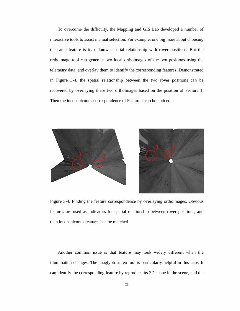
To overcome the difficulty, the Mapping and GIS Lab developed a number of
interactive tools to assist manual selection. For example, one big issue about choosing
the same feature is its unknown spatial relationship with rover positions. But the
orthoimage tool can generate two local orthoimages of the two positions using the
telemetry data, and overlay them to identify the corresponding features. Demonstrated
in Figure 3-4, the spatial relationship between the two rover positions can be
recovered by overlaying these two orthoimages based on the position of Feature 1.
Then the inconspicuous correspondence of Feature 2 can be noticed.
Figure 3-4. Finding the feature correspondence by overlaying orthoimages. Obvious
features are used as indicators for spatial relationship between rover positions, and
then inconspicuous features can be matched.
Another common issue is that feature may look widely different when the
illumination changes. The anaglyph stereo tool is particularly helpful in this case. It
can identify the corresponding feature by reproduce its 3D shape in the scene, and the

29
shape is irrelevant with the illumination. These tools are used separately or in
combination to identify features depending on the characteristics of the specific
terrain.
Since the cross-site tie point selection involves more than one rover position, the
image combination has wide options. If there are only two rover positions, both
positions will use their own stereo pairs to calculate the coordinates of tie points, so
that the offset between two sets of coordinates can be eliminated in the bundle
adjustment. But if there are more than two positions, any two positions can be
combined to generate stereo pairs as long as the images have overlapping areas. Then
the bundle adjustment may adjust these two positions as an analogous rigid body to
other positions. The primary difference between these two patterns is the length of the
baseline between the left camera and the right camera. The baseline in the first
condition is fixed since the cameras are installed on the PMA, so it is named as hard
baseline. On the contrary, the baseline in the second condition is flexible depending
on the image combination, so it is named as wide baseline, or soft baseline.
The baseline length is an important factor to decide the accuracy of the
coordinates of cross-site tie points. Figure 3-5 below illustrates how the baseline
length can affect the accuracy of a feature in Pancam images. Assume that the
matching point in the right image gets an offset of 1 pixel (10 µm × 10µm) in the
across-photograph axis, and the ground point is about 50 m away from cameras. If a
stereo pair with hard-baseline is used to observe this point, the 1 pixel offset can cause
2.6 m offset in the along-photograph direction. However, if two images from two
rover positions that are 5 m from each other are used as a stereo pair, the offset in the
object space can be reduced to 0.15 m. This fact determines what type of baseline
length should be used under different conditions.

30
Figure 3-5. The effect of baseline length on the accuracy of coordinates of tie points.
In the rover localizations for MER mission, cross-site tie points can be selected
using hard-baseline stereo pairs. With the limit of manpower and required timeliness
of the mission, an incremental bundle adjustment is performed in a stepwise manner,
which only involves two adjacent rover positions each time. Therefore, the 3D
coordinates of tie points must be extracted using stereo pairs from both rover
positions separately. The same condition happens to the mapping of some craters.
Santa Maria is a relatively young impact crater, but old enough to collect sand
dunes in its interior. The Compact Reconnaissance Imaging Spectrometer for Mars
(CRISM) data shows indications of hydrated sulfates on the southeast edge of the
Santa Maria Crater (Kremer, 2010). And the sand dunes at the bottom also hold clues
to the past and present climate processes on Mars. Its scientific value cannot be dug
out without a detailed terrain model. Therefore, the traverse around Santa Maria was

31
specially designed to fulfill the mapping task.
Besides Santa Maria, one large crater, Endurance, was mapped completely by the
Mapping and GIS Lab. Another mapping that involves multiple rover positions is for
the Duck Bay at Victoria Crater. By comparing these three mapping cases with
multiple rover positions, it is not difficult to observe that the rover positions around
Santa Maria are grouped into the western part and the eastern part, in which the
positions of Site 1, 2, 4, and 5 are planned specifically for wide-baseline mapping.
This special distribution provides an unprecedented opportunity for us to study the
wide-baseline tie point selection.
(a) (b)
Continued
Figure 3-6. The distribution of rover positions near (a) Endurance, (b) Duck Bay at
Victoria, and (c) Santa Maria.

32
Figure 3-6 continued
(c)
In the case of mapping Santa Maria, the key to success is to link the western
positions with the east positions by cross-site tie points. The best option is to select
these points in the middle of the crater so that they are not too far or too close to either
side. However, if the traditional hard-baseline selection is used, it may cause a
systematic bias among sets of tie points because of the reliable distance of
Pancam/Navcam images. And this bias will be carried to the initial rover positions
through rigid transformation, which will be discussed later, and then affect the rover
localization, as illustrated in the following Figure 3-7.

33
Figure 3-7. The result of rigid transformation when hard-baseline cross-site tie points
are used. The dots in four different colors are tie points observed from those four
rover positions. The black crosses are telemetry rover positions. The red crosses are
the true rover positions. The green crosses are the rover positions following the
pattern of the hard-baseline tie points.
The solution to this issue is to construct stereo pairs with wide baseline between
two rover positions and use their camera parameters to calculate the 3D coordinates of
tie points. For example, the left images in Site 1 and Site 2 that have overlaps are
selected to form stereo pairs, so do the left images in Site 4 and Site 5. Instead of
having four sets of hard-baseline cross-site tie points from four rover positions, this
wide-baseline method only generates two sets of coordinates for the tie points, and
they are with a much higher accuracy. Figure 3-8 and 3-9 present the structure and its
advantage over the hard-baseline method. As can be seen, the pattern between two
sets of points is consistent with the pattern between the telemetry rover positions and
the true positions.

34
Figure 3-8. The construction of wide-baseline tie point selection.
Figure 3-9. The result of rigid transformation when wide-baseline cross-site tie points
are used. The red dots are observed from Site 1 and 2 in the western side, and the blue
dots are from Site 4 and 5 in the eastern side.
After the selection of intra-, inter-, and cross-site tie points, either by
hard-baseline method or wide-baseline method, it is ready to link all images taken
from different rover position together to generate the image network. In this network,
each image is a node in a connected graph, and the tie points function as paths among

35
nodes.
This chapter introduced three types of tie points for constructing image network.
Intra- and inter-site tie points can be selected automatically with a systematic process,
but cross-site tie points are often selected manually due to the significant differences
in viewing angles, resolutions, and distances between images and rover positions.
With the help of interactive tools, the difficulty of tie point selection may be
simplified. To ensure the accuracy of coordinates of tie points, different combinations
of image are used to compose soft baseline, or wide baseline. The experiment at Santa
Maria Crater is the first successful attempt of this method, and the experience can be
used for reference in the future mapping.

36
Chapter4:IntegratedBundleAdjustment
Bundle adjustment is almost always used as a step in every feature-based 3D
reconstruction algorithm. It is the problem of refining a visual reconstruction to
produce jointly optimal 3D structure and viewing parameter (camera pose and/or
calibration) estimates (Trigg, et al, 1999). Bundle adjustment is the most important
step in the Martian crater mapping. All the following processes must be built on the
success of bundle adjustment. In the previous MER mission operation, a step-wise
incremental bundle adjustment was used because of the timeliness and the lack of
manpower. In recent studies, a new integrated bundle adjustment that utilizing both
orbital and ground data is developed. Chapter 4 is going to discuss the general theory
behind bundle adjustment and the practice of both incremental and integrated manners,
and then to explore their strengths and weaknesses.
4.1Theoryofbundleadjustment
Bundle adjustment was originally conceived in the field of photogrammetry
during 1950s and has been applied increasingly to computer vision, industrial
metrology, surveying, geodesy and many other fields. Bundle adjustment is a problem
about geometric parameter estimation including the coordinates of ground features,
the interior and exterior orientation parameters of cameras. The purpose of bundle
adjustment is to find a set of the parameters that minimizing the model fitting error
described by certain cost functions, and thus to give good prediction of the location of
the observed points in a set of images. Like other adjustment computations, classical
37
bundle adjustment is formulated as a nonlinear least square problem. The cost
function is assumed to be quadratic in the feature re-projection errors, and robustness
is provided by explicit outlier filtering.
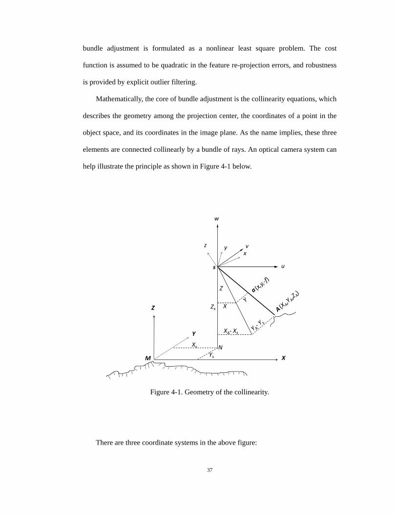
Mathematically, the core of bundle adjustment is the collinearity equations, which
describes the geometry among the projection center, the coordinates of a point in the
object space, and its coordinates in the image plane. As the name implies, these three
elements are connected collinearly by a bundle of rays. An optical camera system can
help illustrate the principle as shown in Figure 4-1 below.
Figure 4-1. Geometry of the collinearity.
There are three coordinate systems in the above figure:

38
(1) The image space coordinate system. Its origin is the projection center S (the
camera). The z axis coincides with the principal optic axis while the positive
direction is against the photographic direction. The x and y axes are parallel to
the x and y axes in the image plane coordinate system. This system is represented
by xyzS .
(2) The object space coordinate system. The origin is at an arbitrarily specified
location M . The Z axis coincides with the zenith directions at the origin of the
coordinate system. Then the X and Y axes form a horizontal plane, whose
directions can be determined by a certain ground coordinate system, for example, the
direction of the base line between two cameras, or the flight direction. This system is
denoted by XYZM .
(3) The image auxiliary coordinate system. Its origin is also S , but the axes are
rotated to be parallel to those of object space coordinate system. Angle rotates
around the axis SY ; Angle rotates around the axis SX ; Angle rotates
around the SZ . This coordinate system is denoted by uvwS .
Given a ground point A , its coordinates in XYZM is ),,( AAA ZYX , and its
image point has the coordinates of ),,( fyx with respect to xyzS and
),,( ZYX with respect to uvwS . The coordinates of the projection center S in
XYZM is ),,( SSS ZYX . The following equations can be deduced from the
similar triangles in Figure 4-1:
1
SASASA ZZ
Z
YY
Y
XX
X
(4-1)
in which is a constant scaling. The equations can also be written in the matrix
format as:

39
SA
SA
SA
ZZ
YY
XX
Z
Y
X
1
(4-2)
Besides that, the rotation between the image space coordinate system and the
image auxiliary coordinate system can be used to establish the following equation:
f
y
x
ccc
bbb
aaa
f
y
x
R
Z
Y
X
321
321
321
(4-3)
in which matrix R is the rotation matrix whose elements are functions of the three
rotation angles:
cos0sin
010
sin0cos
cossin0
sincos0
001
100
0cossin
0sincos
RRRR
(4-4)
Combining equations (4-1) to (4-4), the collinearity equation is given as follows:
)()()(
)()()(
)()()(
)()()(
333
2220
333
1110
SASASA
SASASAa
SASASA
SASASAa
ZZcYYbXXa
ZZcYYbXXafyyy
ZZcYYbXXa
ZZcYYbXXafxxx
(4-5)
in which ),( aa yx and ),( 00 yx are the image coordinates of Point A and the
principle point S in a coordinate system whose origin is the image center.
As can be seen from Equation (4-5), each point can construct two collinear
equations with variables. According to different applications, certain variables are
known, while some others need to be calculated. However, the interior orientation
parameters, including f , 0x , and 0y , are considered as known in most conditions
since they are measured in the laboratory calibration process and are rarely changed.
The image coordinates of points can also be known through direct measurement from
images. In the application of Martian crater mapping, the unknowns include the

40
exterior orientation parameters of all the Pancam / Navcam images in the image
network, and the ground coordinates of all the tie points.
Good initial values are essential to get the optimal solution to the collinearity
equations. The attitude information of images from the telemetry data within one
rover position is generally consistent and can be used directly as initial values.
However, the coordinates of same features observed from different positions are often
inconsistent with each other and thus must be pre-processed for bundle adjustment.
This inconsistency comes from the factors such as wheel slippage, IMU angular drift,
and other navigation errors. Since these factors exist through the whole traverse in a
systematic manner, a rigid transformation (translation and rotation without scaling) is
applied to all relevant rover positions except for the reference position with the help
of cross-site tie points. A least-square-based algorithm is iterated to estimate the
optimal transformation model and screen the outliers in tie points. The transformation
parameters are determined only by tie points with residual errors less than 1 m in all
X-Y-Z directions. The exterior orientation parameters and the ground coordinates of
features will be much more consistent and can be used as initial values after this
transformation.
As can be seen from Equation (4-5), the collinearity equations are non-linear
functions with respect to most of the parameters and variables. The Linearization is a
good solution for simplifying computation, solving unknowns simultaneously and
enabling the least squares to minimize the re-projection errors. The classical
linearization algorithm is to use the Taylor series expansion to derivate the linear
form.
4.2IncrementalBundleAdjustment

41
The incremental bundle adjustment was designed for the demand of daily
localization task in the MER mission. The rovers move along their traverses and take
images incrementally sol by sol. These images generate a special chain rather than a
network. For a long traverse, the amount of images involved is extremely huge, which
causes two issues:
(1) The tie points between positions cannot provide strong connection in
recovering the relative orientation between rover positions. Tie points can only be
selected within the reliable distance of cameras if hard-baseline method is used for
selection, which limits their ability of binding multiple positions at the same time.
Therefore, it is difficult to find an optimal solution for all the positions at the same
time, let alone that the tie points may not be as precise as required because of the lack
of identifiable features or the long distance between locations.
(2) It is too computationally expensive to involve the entire image network for
the localization of each rover position. The time is highly restricted for everyday data
acquisition, data processing, rover localization and map submission. In addition, the
manual cross-site tie point selection is quite time consuming even for an experienced
operator. As the traverse expands sol by sol, it is more and more impossible to take the
entire network into account.
In an ideal condition, a sequential computing process allows adding/deleting
variables, known or unknown, at any node of the image network, and updates the
solution with the alterations, so that the final results are the same with those of a
simultaneous process (Gruen, 1985). In consideration of the nature of daily operation
and the advantage of sequential computing techniques, an incremental bundle
adjustment model was built up for the special application in MER mission (Li et al.,
2002; Ma et al., 2001).

42
This bundle adjustment model is implemented using the Kalman filter form. At
each new rover position, the unknown parameters are estimated with respect to its
previous position. For the bundle adjusted positions, the parameters will be
re-calculated if new images are available, otherwise the parameters keep unchanged.
As long as there are sufficient images with identifiable features to guarantee the
quality of tie points, this incremental bundle adjustment can obtain a similar solution
with the result of a simultaneous bundle adjustment.
In the operation of MER mission, incremental bundle adjustment is always
performed in a stepwise manner to locate the Spirit rover, and the result demonstrates
that the incremental BA is able to correct significant localization errors (Li, et al.,
2011). However, this success cannot be reproduced in localizing the Opportunity rover.
The reason of this distinct result generally falls into two categories:
(1) Landform diversity. The land covers are quite disparate in Gusev Crater and
Meridiani Planum. Gusev Crater is covered by plenty of rocks, which are perfect
candidates for tie points. On the contrary, Meridiani Planum is full of smooth sand
dunes without many significant features (Figure 4-2). In addition, the terrain of
Meridiani Planum is much plainer than Gusev Crater, which makes distinguishing
features a more difficult task. Therefore the number and quality of tie points in the
operation of Opportunity rover are hard to predict.

43
Figure 4-2. Typical landforms in Gusev Crater and Meridiani Planum. The left image
was taken by Spirit at Site 3100 in Sol 105. The right image was taken by Opportunity
at Site 5000 in Sol 399.
(2) Connectivity of image network. Statistical data in Figure 4-3 shows that the
average drive distance of Spirit rover within each sol is 8.13 m with the standard
deviation of 13.83 m. This length is within the reliable distance of both Navcam and
Pancam, and hence is beneficial to cross-site tie point selection. Meanwhile, the mean
drive distance of Opportunity rover within each sol is 22.78 m with the standard
deviation of 35.77 m. This flexible range is very risky for tie point selection when
Navcam is the only data source, sometimes even risky for Pancam images. If few
cross-site tie points are found between two adjacent rover positions, the connectivity
of image network is weak, and the bundle adjustment may derive wrong results.

44
Figure 4-3. The histograms of traverse in Gusev Crater and Meridiani Planum.
In summary, as a bundle adjustment algorithm that heritages thoughts of
sequential algorithms, incremental bundle adjustment is effective and accurate for
rover localization in MER mission. However, the precision is highly subject to the
quality of tie points, especially when the connectivity of image network is weak. The
errors in the BA of one single position will be accumulated in all the following
positions, until new data is available to update the BA of the first position. In the
application of Martian crater mapping, the biggest problem this error accumulation
may cause is to distort the crater in the along-photography direction.

45
4.3IntegratedBundleAdjustment
To reduce error propagation experienced in incremental BA due to the insufficient
number of features and lengthy drives, an integrated bundle adjustment method has
been developed to bring orbital data in the BA process as well as to adjust multiple
rover positions simultaneously.
As introduced in Chapter 2, HiRISE imagery has resolution of 0.25 m – 0.3 m,
which is the highest until now in orbital images on Mars. This resolution is sufficient
to recognize big rocks and other features on the Martian surface. Meanwhile, the
nature of orbital imagery decides small distortion in a relatively small area that covers
a crater. This distortion is further removed in the orthoimages generated with stereo
images. With the nature of high resolution and small distortion, HiRISE orthoimages
are commendable reference for initial values in the bundle adjustment.
The contribution of HiRISE orthoimage to the initial values comes from two
aspects: the rover localization and the ground positions of tie points. As introduced in
Section 4.2, adjacent rover positions are often linked weakly by insufficient tie points
in Meridiani Planum, which means that the number of cross-site tie points is not large
enough to ignore the disturbance from outliers. This disturbance is going to affect the
result of rigid transformation and provide bad initial rover positions. This
phenomenon is mostly determined by the nature of point-based matching. However, if
an area-based matching is used instead of point-based matching, the situation can be
improved much. The solution is to compare the features, such as ridges, rocks, and
rims, as a whole in HiRISE orthoimage and the ground-based local orthoimage. By
registering local features, a HiRISE orthoimage and a ground-based local orthoimage
within one rover position can be precisely overlaid, and then the rover position at the

46
imaging center on the ground-based orthoimage can be determined on the HiRISE
orthoimage as Figure 4-4 shows below.
Figure 4-4. Initialization of a rover position through feature comparison between
HiRISE orthoimage and ground-based orthoimage.
The second contribution of HiRISE orthoimage is to provide good initial values
of the coordinates of tie points. Using wide-baseline method could lower the risk of
getting bad distant cross-site tie points, but errors can still exist in the coordinates of
those points because of the subjectivity in the manual selection, the residual error in
the adjusted camera parameters, or other factors. To further improve the accuracy of
these coordinates, the HiRISE orthoimage is used as a reference. Only features that
can be seen in the orbital images are selected as cross-site tie points. For any distant
tie points whose image coordinate are already verified as accurate, if there is still a
large difference between the 3D coordinates calculated from the ground images and
those measured from the orbital orthoimage, the difference is regarded as the result of
inconsistent relationship among rover positions, and the orbital coordinates are

47
considered to be more reliable and are used as the initial values in the following
bundle adjustment.
By the contribution of HiRISE orthoimage, the link within the image network is
highly strengthened. With good initial values of rover positions and coordinates of tie
points, a bundle adjustment is performed over all related rover positions
simultaneously, so that the whole image network can achieve the optimal solution as a
whole. Experimental results show that this simultaneous bundle adjustment with
integrated data input can provide much better attitude and position revision than the
incremental bundle adjustment with only ground data.
However, the current integration of orbital data is still in the initial phase with a
number of issues under continuous research. One primary issue is the extraction of
elevations of tie points from orbital products. In the current experiment, only the
horizontal coordinates of tie points measured from the orbital orthoimages are used in
the integrated bundle adjustment. Ideally, the elevations of tie points from orbital
products would also contribute much to the strong connection of image network
because that they are relatively consistent with each other in a large area, especially
when the elevation is further controlled by MOLA data. However, they are not
extracted from the orbital DTM or utilized in the bundle adjustment. The crucial
reason is the unreliability of the quality of present DTM in small areas such as a crater.
As can be observed in Figure 4-5, shadows and shadings are quite common in HiRISE
images of Martian craters, especially the ones with certain depth under low sun angle.
Image matching process is almost impossible to be fulfilled in these dark areas. And
without matching features, the stereo pair cannot provide valid 3D information.
Figure 4-6 shows an example of the orbital DTM at Santa Maria crater comparing
with the DTM generated in the proposed method. The inconsistency is quite

48
inescapable in the shading area. A failure is expectable if the bundle adjustment
employs the elevations of tie points from this DTM.
(a) (b)
Continued
Figure 4-5. Shadows and shadings in HiRISE images of Martian craters. They are
clipped from the HiRISE images: (a) TRA_000873_1415, a crater in Noachis Terra,
(b) ESP_025680_1350, a crater in Terra Cimmeria, (c) TRA_000873_1780, Victoria
Crater at Meridiani Planum. (Image Source: HiRISE)

49
Figure 4-5 continued
(c)
Figure 4-6. The comparison between the DTMs generated from HiRISE images (the
above one) and the one generated with proposed method (the bottom one).
4.4EvaluationofBundleAdjustmentResults
It is risky to generate digital terrain models and other topographic mapping
products without evaluating the results of the bundle adjustment because of the

50
possibility of remaining inconsistencies. Since no absolute ground control is available
on Mars, it is impossible to evaluate the accuracy of the bundle adjustment using the
conventional method of comparing the adjusted positions with ground truth. Instead,
the accuracy was evaluated by looking at two aspects: the level of consistency among
multiple rover positions, and the comparison of bundle adjustment localization results
with orbital products.
The consistency among multiple rover positions is checked by comparing the 3D
coordinates of points which are calculated using positioning information of different
rover positions. These points may not be seen in the orbital image, but they need to be
observed in more than one rover position. Then their 3D coordinates are calculated
using either the hard-baseline method or the wide-baseline method, according to
different circumstances. The offsets among sets of coordinates from different
positions indicate the quality of bundle adjustment. Figure 4-7 shows one of these
comparison results at Santa Maria Crater. The red dots come from two sites in the
west using wide-baseline method. Blue dots come from two sites in the east also using
wide-baseline method. Apparently, the inconsistency before bundle adjustment in the
left image is reduced significantly after bundle adjustment in the right image. Detailed
statistic information can be found in Table 4-1.

51
(a) Features before bundle adjustment. (b) Features after bundle adjustment.
Figure 4-7. Inconsistencies between features among multiple rover positions before
and after bundle adjustment. Black crosses are the telemetry rover positions. Red
triangles are the rover positions based on the bundle-adjustment results.
Offset Before BA Offset After BA
Point ID X Y Z X Y Z
0 -2.34 5.21 1.58 -0.56 -0.66 -0.33
1 -2.57 5.55 1.36 0.17 -0.29 -0.19
2 -2.63 5.41 2.11 -0.39 -0.46 0.39
3 -3.57 5.46 1.92 -0.94 -0.33 0.31
4 -2.06 5.36 1.82 0.40 -0.08 -0.01
5 -0.63 5.91 1.88 0.77 0.14 0.05
7 -2.79 5.83 1.06 0.13 -0.28 -0.16
Continued
Table 4-1. The statistics of the inconsistencies between features among multiple rover
positions before and after bundle adjustment.

52
Table 4-1 continued
8 -1.14 5.91 1.57 -0.24 0.28 -0.08
9 -0.98 5.65 1.99 1.61 -0.24 0.24
11 -1.71 5.60 1.51 -0.11 0.16 -0.25
12 -3.55 4.37 1.45 -0.33 -1.37 -0.23
13 -3.14 4.37 1.70 -0.58 -1.05 0.01
In the experiment at Santa Maria Crater, the 3D coordinates of 151
manually-chosen tie points were measured from all images that contain the features,
and then the offset for each point after bundle adjustment was calculated. Result
shows that 88.7% of the points have an offset of less than 1 m. The minimum of those
offsets is 0.05 m, the maximum is 1.52 m, and the average offset is 0.53 m.
Another evidence of the dependability of the bundle adjustment is that the rover
positions and features measured from the adjusted ground images are consistent with
the same positions and features observed from the orbital orthoimage. This evaluation
requires features that can be observed in both orbital image and ground images.
Figure 4-8 illustrates a good comparison result at Santa Maria Crater. Red dots
represent ground-image-based features after bundle adjustment. Yellow dots represent
the same features measured from the orbital orthoimage. Meanwhile, the red triangles
are the rover positions based on bundle adjustment results, and the yellow triangles
are the rover positions measured from HiRISE orthoimage. After bundle adjustment,
the minimum of those offsets is 0.31 m, the maximum is 1.66 m, and the average
offset is 0.74 m. More detailed statistic information about the compared features is
listed in Table 4-2.

53
Figure 4-8. The consistency of rover positions and features between bundle adjusted
ground images and orbital orthoimage.
Positions in HiRISE Positions in Ground Offset
Point ID X Y X Y X Y
0 4,491.79 -12,546.28 4491.71 -12546.23 -0.08 0.05
1 4,517.97 -12,537.74 4516.99 -12538.54 -0.98 -0.80
2 4,494.57 -12,556.36 4494.70 -12556.16 0.13 0.20
3 4,532.82 -12,543.54 4532.32 -12543.09 -0.50 0.45
4 4,532.62 -12,554.14 4532.52 -12552.50 -0.10 1.64
Continued
Table 4-2. The statistics of the consistency of features and rover positions between
adjusted ground images and orbital orthoimage.

54
Table 4-2 continued
5 4,556.77 -12,565.65 4555.66 -12565.58 -1.11 0.07
6 4,545.27 -12,610.18 4544.50 -12610.85 -0.77 -0.67
7 4,532.96 -12,594.37 4532.54 -12594.72 -0.42 -0.35
8 4,507.60 -12,600.89 4506.92 -12600.45 -0.68 0.44
9 4,519.64 -12,609.50 4520.05 -12608.74 0.41 0.76
10 4,513.59 -12,617.78 4513.55 -12617.18 -0.04 0.60
11 4,493.14 -12,610.78 4494.01 -12610.31 0.87 0.47
12 4,471.24 -12,559.56 4470.94 -12559.51 -0.30 0.05
Site ID X Y X Y X Y
1 4648.10 -13301.33 4648.10 -13301.33 0 0
2 4649.75 -13306.61 4650.07 -13307.48 0.32 -0.87
3 4744.96 -13332.90 4743.44 -13333.31 -1.52 -0.38
4 4743.96 -13322.58 4743.93 -13322.13 -0.03 0.45
5 4745.07 -13317.64 4744.92 -13317.37 -0.15 0.27
The above criteria can be used alone or in combination to check the quality of the
bundle adjustment before it was applied to crater mapping.
In this chapter, the basic theory of bundle adjustment and its two practical
implementation manners for different circumstances are introduced. The incremental
bundle adjustment is designed mainly to meet the timely limitation in the rover
localization task in the MER mission. It works well when sufficient, well-distributed
tie points can be found between adjacent rover positions. However, due to the
different landforms and other factors, this successful example in Gusev Crater cannot

55
be repeated in Meridiani Planum. To eliminate the error accumulation that may be
caused by incremental bundle adjustment, an integrated bundle adjustment is designed
to involve orbital data in the process. Despite of the lack of features in Meridiani
Planum, the initial values of rover positions can still be ensured by HiRISE
orthoimage. In addition, the coordinates of tie points can also be supervised by orbital
images. Although this integrated method is still under research, the evaluation reveals
its great potential for Martian crater mapping.

56
Chapter5:MappingProductGeneration
After the bundle adjustment is performed and evaluated, the attitudes and
positions of all cameras agree with each other and get prepared to extract dense
matching points within the craters to build the terrain model. Besides the DTM, which
is the most fundamental mapping products, other products will also be derived,
including the orthoimage, the slope map, the contour map, and so on. However, these
mapping products cannot be generated without the basic DTM. Therefore, this chapter
will devote itself to the detailed process of DTM generation since it is the bed stone
for all other mapping products. Some discussion will be put forward about interest
point extraction in featureless area. A brief introduction will also be given to the
generation of the orthoimage, including the back-projection and other image
processing methods. Since other derivatives such as the contour map and the slope
map can be easily generated by commercial software such as ArcMap, few
discussions will be put on them.
5.1GenerationofDTM
DTM generation includes: (1) dense interest point matching, (2) 3D coordinate
calculation of the matched points, and (3) DTM interpolation. In these three steps,
dense interest-point matching and 3D coordinate calculation of the matched points are
related with each other very closely, and they form the fundamental part of the DTM
generation. Based on the theoretic research discussed before and the empirical

57
experience accumulated in these years, hard-baseline and wide-baseline techniques
are both used to implement these two tasks under different conditions.
There is no strict law on which method should be used in which conditions, but
some rules may help for the decision: (1) the dimension of the crater, (2) the distance
between the crater and the camera, and (3) the available image type. All the three
rules are defined in a relative way. For example, the definition of a small crater in this
research varies depending on what type of rover images were taken around the crater.
If both Pancam images and Navcam images are available to map the crater, a small
crater could be as large as about 60 m in diameter. But if Navcam images are the only
data source, the diameter should not be over 30 m for the purpose of accurate
mapping. These diameters are determined by the reliable distances of cameras. In
addition, the distance from the crater to the camera is also critical to determine the
dense matching method. Even if the crater itself is a small one, if it is far from the
rover position, a hard-baseline method may not have a good performance at the far
end of the crater since it is outside the reliable distance. In a summary, hard-baseline
method is a simple but effective choice for craters within the reliable distances of the
cameras, while wide-baseline mapping is used mainly to cover areas that are blocked
by crater walls near sites or when points are more distant than the reliable mapping
distance found for hard-baseline mapping. Figure 5-1 gives a simple illustration on
this principle.

58
Figure 5-1. “Rules” for choosing dense matching method.
However, a phenomenon has been more and more noticeable in our research
these days, which cannot be classified using the above rules. Following the drive plan,
the rover may pass by an interesting crater, taking a few images of the crater in one
position without making a close observation. As a result, the near end of the crater
will be blocked by its own rim while no images from other positions were available to
observe this blocked area. Figure 5-2 shows an example at Geographe Crater in
Meridiani Planum. The diameter of this crater is about 13 m, but the distance to the
rover is about 23 m, which makes part of it invisible. However, this crater was only
observed in Site 4700, so this crater cannot be mapped using the wide-baseline
method according to the above rules. With the help of orbital image, the blocked area
may be completed. However, the resolution will not be as high as the one using
ground images. A more critical issue is that a precise bundle adjustment must be
implemented simultaneously on both orbital images and ground images to guarantee a
smooth mosaic, which is still very challenging so far. This topic is our priority in the
future work.

59
Figure 5-2. Geographe Crater with its blocked area.
Similar with tie point selection, the dense interest point matching is also divided
into the automatic process and the inevitable manual process. Most of the automatic
process is implemented by the same method used in tie point selection: Förstner
operator and NCCC. This combination works well in the areas with rich features, but
it performs poor in the relatively smooth areas, such as the sand dunes in the bottom
of many Martian craters. Yet the sand dune is an important subject in the research of
Mars. Scientists believe that those unusual ripples hold clues to the past and present
climate processes on Mars. Since they are an outer layer composed of granule-sized
material ranging from about 2 mm - 5 mm (Williams, et al., 2002), they look so
smooth even from the high-resolution rover images that very few features can be
found in the troughs. Another factor affecting the performance of the Förstner
operator and NCCC is the very different viewing angles at sand dune area. As
mentioned in previous chapters, sandy areas are the most dangerous area for rovers
because of the possibility of stuck of wheels. With that principle in mind, the rover
almost never took the risk of going into craters, not to mention the sand dunes in the
middle of the craters. Therefore, the sand dune is always far from rover positions and
cannot be mapped in the hard-baseline way. Only one option is left in this condition,
to use wide-baseline mapping and to live with the different viewing angles.

60
One beneficial solution to this dilemma is to use Scale Invariant Feature
Transform (SIFT) algorithm at the sandy areas to find as many matching point
candidates as possible. This algorithm was developed by Lowe (1999; 2004) and has
been demonstrated by numerous papers as superior to other feature matching
algorithms in scale and affine variant regions. Since this algorithm is already known
to everyone in the computer vision related field, the technical details will not be
introduced again here. With the help of SIFT algorithm, the features can be extracted
more from the troughs rather than along the ridges, which is necessary to map the
detailed shape of the sand dune area. Otherwise, if all features are extracted on the
ridges, the elevation of the sand dune will lose the small variations.
Although SIFT algorithm is known for its accuracy in feature extraction, it will
still have many outliers left because the smoothness of the sandy area, and much
manual editing must be involved to delete the mismatches and add new matching
points. It is very onerous even for a very experienced operator, but it is also very
necessary step before any better automatic matching algorithm appears. Figure 5-3
plots the dense matching points over the HiRISE orthoimage in the Santa Maria
Crater, including automatic ones and manual ones. Manual points are added as many
as possible to make sure that all obvious features in the crater are covered. However,
some smooth areas on the wall are still not covered by any points. Considering that
these smooth areas have a relatively simple slope, the mapping quality will not be
affected too much.

61
Figure 5-3. The dense matching points in Santa Maria Crater.
With sufficient matching points, a DTM can be generated easily using
interpolation methods, such as Kriging, Natural Neighbor, and Spline provided in
ArcMap. In this study, the Natural Neighbor method is used to get a relatively smooth
surface. The DTM of Santa Maria Crater is shown in Figure 5-4 with a resolution of
0.1 m. Figure 5-5 gives a detailed DTM in the sand dune area. Compared with
HiRISE orthoimage, it is easy to see that the ridges and troughs in the DTM are very
close to “the ground truth”.

62
Figure 5-4. Feature Comparison between the DTM of Santa Maria Crater and the
HiRISE orthoimage. The above image is the HiRISE orthoimage of Santa Maria. The
bottom image is the DTM generated from the proposed method.

63
Figure 5-5. The detailed DTM at the sand dune area of Santa Maria Crater.
5.2OtherTopographicProductMapping
Although the DTM is good at presenting the terrain, it is not good at reflecting
the ground materials, from which an experienced researcher can dig out much
information about the geological structure, climate change, and even evidence of
water existence. Therefore, an orthoimage is necessary for the research purpose.
Points in the DTM are back-projected to the ground images taken from multiple
positions to get corresponding pixel values. The adjusted camera parameters are used
to calculate the coordinates in image plane from the 3D coordinates in the object
space. In principle, the image pixel taken from the nearest rover position should be
used for the pixel value, because the calculation accuracy increases when the distance
gets smaller and smaller. To a crater with certain depth, most part of the crater can be
processed following this rule. But unlike flat areas, the rim of a crater can block the
rover from observing the nearby features (Figure 5-6). If following the same rule in
this condition, pixels on the boundary of the blocked area will be used as substitutes

64
and cause blunder in the orthoimage, as Figure 5-7 shows. The red polygon marks a
blocked area which cannot be observed from western positions, but the software still
gives pixel values from images of the rocks on the western cliff just because those
pixels are closest to the blocked area.
Figure 5-6. The blocked areas in crater mapping.
Figure 5-7. Using the nearest pixels causes wrong filling in blocked areas.

65
To eliminate these exceptions, the image pixels taken from the opposite sides are
used for the final pixel values. First of all, the program generates the orthoimage
automatically without any human intervention. Then the images taken close to the
blocked areas are removed from the database, so that the software is forced to use the
images from distant cameras. Take Santa Maria Crater for an example, images from
Site 4 and 5 are used to map the blocked areas in the western part of the crater, while
images from Site 1 and 2 are used for the blocked areas in the eastern part.
Another issue in generating orthoimage is the coherence of the brightness among
different ground images. As can be seen in Figure 5-7, the sand dune area is obviously
brighter than other areas of this crater. The rocks on the cliff are also always brighter
than their surroundings. This is an inevitable phenomenon caused by the exposure
characteristics of the cameras onboard the rovers, which may not affect the scientific
research, but cannot give observers a good visualization because it splits the crater in
pieces. It is not realistic to pre-process all those images to get a similar brightness,
especially when they are separated from each other, but a post-processing is quite
simple and effective. The Photoshop provides the function of adjusting brightness
with real-time preview, so the distinguished areas can be chosen carefully and be
adjusted until the operator sees different pieces merging together. Figure 5-8 shows
the brightness at sand dune area before and after this adjustment.

66
Figure 5-8. The brightness adjustment in sand dune area of Santa Maria Crater. The
left image is before adjustment, and the right image is after adjustment.
The complete orthoimage will look quite smooth after all those circumspect
image processing steps. Figure 5-9 illustrates how the final orthoimage is improved
from the raw version. This improvement also demonstrates the necessity of the
post-processing in orthoimage generation.
Figure 5-9. Orthoimage of Santa Maria Crater before and after image post-processing.
The resolution is 0.1 m.

67
The quality of the above orthoimage can be evaluated by comparing it to the
HiRISE orthoimage. In Figure 5-10, features in both orthoimages are quite matching
with each other.
(a) Orthoimage from HiRISE (b) Orthoimage from proposed method
Figure 5-10. Comparison between orthoimages generated via different methods.
Since Santa Maria Crater is not in a regularly circular shape, the dimension is
compared with HiRISE orthoimage by measuring the diameter in northing and easting
directions using the same features as the end points. Table 5-1 lists the result of
comparison. The orthoimage/DTM generated by the proposed method have very
similar dimension with the HiRISE product.

68
Northing Easting
HiRISE 95.12 m 91.83 m
New Method 95.33 m 91.95 m
Table 5-1. The comparison on the dimension of Santa Maria Crater.
Other mapping products, such as the contour map and the slope map can be
derived easily using commercial GIS software. As per the Mars Data Analysis
Program (MDAP) proposal, the positions of Alpha Particle X-Ray Spectrometer
(APXS) data and Microscopic Imager (MI) images are also adjusted using the
bundle-adjusted rover positions and then plotted to the terrain models. Figure 5-11 is a
summary of the product set at Santa Maria Crater. No MI images were taken around
Santa Maria, so there is no legend in this summary.

69
Figure 5-11. The product set at Santa Maria Crater.

70
Chapter6:Conclusions
Surrounding the topic of Martian crater mapping, this thesis followed the
workflow in Chapter 1 and introduced all the important steps leading to a successful
mapping and the theories behind those steps.
Mars draws more and more attention in these years because it is the only planet
that may support lives, except for the Earth. High-quality surface mapping can
provide detailed data for scientists to analyze the geological environment of Mars, and
to look for the evidence of water existence, which is the most direct proof for the
possibility of life on Mars.
With the help of HiRISE data, it is now possible to integrate the orbital data and
the ground data for high-resolution mapping. HiRISE data contributes in the image
network construction by providing reference on the position of tie points. HiRISE acts
as the ground truth in the bundle adjustment phase by helping in deciding the initial
values of the rover positions. This integration is still in the initial stage, but more and
more study will be done in the future to utilize HiRISE data in a deeper level. As
mentioned in Chapter 5, our next goal is to bundle adjust the orbital images and
ground images simultaneously. There are plenty of issues to be fixed, but the
integration will definitely reform the whole crater mapping process.
As to the ground data processing, the wide-baseline method is used in the tie
point selection phase for the first time, and proves to be very effective for controlling
the accuracy of distant tie points in the case of Santa Maria Crater mapping.
Experiments in other craters need to be designed to make sure that this method is

71
robust under various conditions. Theoretical analysis is still in demand to support the
realistic practices.
Another important evolution is that the bundle adjustment is not in the step-wise
manner any more in the crater mapping process. Instead, a simultaneous manner with
orbital reference is put forward to acquire more accurate rover position adjustment for
crater mapping. Along with better-controlled tie points, this adjustment turns to be
very successful at Santa Maria Crater. This method will continue the fulfillment in
other large craters listed in the MDAP proposal.
Besides the big improvements above, some algorithms and programs are added in
to the process for better automation and visualization. For instance, the SIFT
algorithm helps automate the dense interest point matching in the featureless areas,
which reduces the amount of manual work. The Photoshop program is used in the
orthoimage generation to solve the issues in mosaicking ground images with different
brightness. Without the help of these useful tools, the high-resolution Martian crater
mapping could have been a much more difficult task.
On one hand, the proposed method proves successful in the case of Santa Maria
Crater and shows great potential in Martian crater mapping. On the other hand, there
are still many questions about its robustness and common adaptability. More
experiences need to be accumulated to give more convincing conclusions. The future
work will focus on the aforementioned issues in this chapter, and try to involve more
scientific analysis upon the mapping products for data mining.

72
References
Ali, K. S., C. A. Vanelli, J. J. Biesiadecki, M. W. Maimone, Y. Cheng, A. M. San
Martin, and J. W. Alexander, 2005. Attitude and Position Estimation on the
Mars Exploration Rovers. 2005 IEEE Conference on Systems, Man, and
Cybernetics, Kona, Hawaii, October, 2005.
Allison, M., and R. Schmunk, 2012. Technical Notes on Mars Solar Time as Adopted
by the Mars 24 Sunclock. NASA. Accessed Sep. 15, 2012,
http://www.giss.nasa.gov/tools/mars24/help/notes.html.
Bell III, J. F., S. W. Squyres, R. E. Arvidson, H. M. Arneson, D. Bass, D. Blaney, N.
Cabrol, W. Calvin, J. Farmer, W. H. Farrand, W. Goetz, M. Golombek, J. A.
Grant, R. Greeley, E. Guinness, A. G. Hayes, M. Y. H. Hubbard, K. E.
Herkenhoff, M. J. Johnson, J. R. Johnson, J. Joseph, K. M. Kinch, M. T.
Lemmon, R. Li, M. B. Madsen, J. N. Maki, M. Malin, E. McCartney, S.
McLennan, H. Y. McSween Jr., D. W. Ming, J. E. Moersch, R. V. Morris, E.
Z. Noe Dobrea, T. J. Parker, J. Proton, J. W. Rice Jr., F. Seelos, J. Soderblom,
L. A. Soderblom, J. N. Sohl-Dickstein, R. J. Sullivan, M. J. Wolff, and A.
Wang, 2004. Pancam Multispectral Imaging Results from the Spirit Rover at
Gusev Crater. Science, 305: 800-806.
Coffey, J., 2008. Atmosphere of Mars. University Today. Accessed Sep. 15, 2012,
http://www.universetoday.com/22587/atmosphere-of-mars/.
Delamere, A., I. Becker, J. Bergstrom, J. Burkepile, J. Day, D. Dorn, D. Gallagher, C.
Hamp, J. Lasco, B. Meiers, A. Sievers, S. Streetman, S. Tarr, M.

73
Tommeraasen, and P. Volmer, 2003. MRO High Resolution Imaging Science
Experiment (HiRISE): Instrument Development. Sixth International
Conference on Mars, Houston, TX, No. 3287.
Förstner, W., and E. Guelch, 1987. A Fast operator for detection and precise location
of distinct points, corners and centers of circular features. ISPRS
Intercommission Workshop on Fast Processing of Photogrammetric Data,
Interlaken, Switzerland, pp. 281-305.
Golombek, M., and T. Parker, 2004. Lander Localization, MER Project Memorandum
(One for Spirit, One for Opportunity). JPL/NASA.
Gruen, A., 1985. Algorithmic Aspects in On-line Triangulation. Photogrammetric
Engineering & Remote Sensing, 51(4): 419-436.
Hwangbo, J. W., 2010. Integration of Orbital and Ground Imagery for Automation of
Rover Localization. PhD dissertation, The Ohio State University.
Jazayeri, I. and C.S. Fraser, 2008. Interest Operators in Close-Range Object
Reconstruction. The International Archives of the Photogrammetry, Remote
Sensing and Spatial Information Sciences, XXXVII (B5): 69-74.
JPL, 2004. Mars Exploration Rover Project Software Interface Specification (SIS)
Rover Motion Counter (RMC) Master File Version 1.0. JPL D-22854.
Kremer, K., 2010. Powerful Mars Orbiter Directs Opportunity to Clays and Hydrated
Minerals. University Today. Accessed July 31, 2012,
http://www.universetoday.com/81789/powerful-mars-orbiter-directs-opportu
nity-to-clays-and-hydrated-minerals/
Li, R., F. Ma, F. Xu, L. H. Matthies, C. F. Olson, and R. E. Arvidson, 2002.
Localization of Mars Rovers Using Descent and Surface-based Image Data.
Journal of Geophysical Research, Planets FIDO Special Issue, Vol. 107 (E11),

74
pp. FIDO 4.1 – FIDO 4.8.
Li, R., K. Di, L. H. Matthies, R. E. Arvidson, W. M. Folkner, and B. A. Archinal, 2004.
Rover Localization and Landing-Site Mapping Technology for the 2003 Mars
Exploration Rover Mission. Photogrammetric Engineering & Remote
Sensing, 70(1): 77-90.
Li, R., S. W. Squyres, R. E. Arvidson, B. A. Archinal, J. Bell, Y. Cheng, L. Crumpler,
D. J. Des Marais, K. Di, T. A. Ely, M. Golombek, E. Graat, J. Grant, J. Guinn,
A. Johnson, R. Greeley, R. L. Kirk, M. Maimone, L. H. Matthies, M. Malin,
T. Parker, M. Sims, L. A. Soderblom, S. Thompson, J. Wang, P. Whelley, and
F. Xu, 2005. Initial Results of Rover Localization and Topographic Mapping
for the 2003 Mars Exploration Rover Mission. Photogrammetric Engineering
& Remote Sensing, 71(10): 1129-1142.
Li, R., S. He, Y. Chen, M. Tang, P. Tang, K. Di, L. Matthies, R. E. Arvidson, S. W.
Squyres, L. S. Crumpler, T. Parker, and M. Sims, 2011. MER Spirit Rover
Localization: Comparison of Ground Image- and Orbital Image-based
Methods and Science Applications. Journal of Geophysical Research,
116(E00F16), doi: 10.1029/2010JE003773.
Lowe, D. G., 1999. Object Recognition from Local Scale-Invariant Features.
Proceedings of the International Conference on Computer Vision, 2:
1150-1157.
Lowe, D. G., 2004. Distinctive Image Features from Scale-Invariant Keypoints.
International Journal on Computer Vision, 60(2): 91-110.
Ma, F., K. Di, R. Li, L. Matthies, and C. Olson, 2001. Incremental Mars Rover
Localization Using Descent and Rover Imagery. ASPRS 2001 Annual
Conference, St. Louis, MO, April 23-27, 11 pp. CD-ROM.

75
Maki, J. N., J. F. Bell III, K. E. Herkenhoff, S. W. Squyres, A. Kiely, M. Klimesh, M.
Schwochert, T. Litwin, R. Willson, A. Johnson, M. Maimone, E.
Baumgartner, A. Collins, M. Wadsworth, S. T. Elliot, A. Dingizian, D. Brown,
E. C. Hagerott, L. Scherr, R. Deen, D. Alexander, and J. Lorre, 2003. Mars
Exploration Rover Engineering Cameras. Journal of Geophysical Research,
108(E12), 24 pp., doi: 10.1029/2003JE002077.
Maki, J., 2003. Mars Exploration Rover Coordinate Systems Relevant to Imaging &
Rover Motion Counter. MER Analyst’s Notebook Producted by NASA’s PDS
Geosciences Node. Accessed July 30, 2012,
http://an.rsl.wustl.edu/mer/merbrowser/browserFr.aspx?tab=res&m=MERB
Malin, M. C., G. E. Danielson, A. P. Ingersoll, H. Masursky, J. Veverka, M. A. Ravine,
and T. A. Soulanille, 1992. Mars Observer Camera. Journal of Geophysical
Research, 97(E5): 7699-7718.
McEwen, A. S., E. M. Eliason, J. W. Bergstrom, N. T. Bridges, C. J. Hansen, W. A.
Delamere, J. A. Grant, V. C. Gulick, K. E. Herkenhoff, L. Keszthelyi, R. L.
Kirk, M. T. Mellon, S. W. Squyres, N. Thomas, and C. M. Weitz, 2007. Mars
Reconnaissance Orbiter’s High Resolution Imaging Science Experiment
(HiRISE). Journal of Geophysical Research, 112(E05S02), 40 pp., doi:
10.1029/2005JE002605.
McEwen, A. S., M. E. Banks, N. Baugh, K. Becker, A. Boyd, J. W. Bergstrom, R. A.
Beyer, E. Bortolini, N. T. Bridges, S. Byrne, B. Castalia, F. C. Chuang, L. S.
Crumpler, I. Daubar, A. K. Davatzes, D. G. Deardorff, A. DeJong, W. A.
Delamere, E. N. Dobrea, C. M. Dundas, E. M. Eliason, Y. Espinoza, A.
Fennema, K. E. Fishbaugh, T. Forrester, P. E. Geissler, J. A. Grant, J. L.
Griffes, J. P. Grotzinger, V. C. Gulick, C. J. Hansen, K. E. Herkenhoff, R.

76
Heyd, W. L. Jaeger, D. Jones, B. Kanefsky, L. Keszthelyi, R. King, R. L.
Kirk, K. J. Kolb, J. Lasco, A. Lefort, R. Leis, K. W. Lewis, S.
Martinez-Alonso, S. Mattson, G. McArthur, M. T. Mellon, J. M. Metz, M. P.
Milazzo, R. E. Milliken, T. Motazedian, C. H. Okubo, A. Ortiz, A. J.
Philippoff, J. Plassmann, A. Polit, P. S. Russell, C. Schaller, M. L. Searls, T.
Spriggs, S. W. Squyres, S. Tarr, N. Thomas, B. J. Thomson, L. L. Tornabene,
C. V. Houten, C. Verba, C. M. Weitz, and J. J. Wray, 2010. The High
Resolution Imaging Science Experiment (HiRISE) during MRO’s Primary
Science Phase (PSP). Icarus 205 (2010): 2-37.
NASA, 2010. Microsoft and NASA Bring Mars Down to Earth Through the
WorldWide Telescope. NASA. Accessed July 29, 2012,
http://www.nasa.gov/topics/nasalife/features/microsoft_ww_telescope.html.
Parker, T., M. Malin, M. Golombek, T. Duxbury, A. Johnson, J. Guinn, T. McElrath, R.
Kirk, B. Archinal, L. Soderblom, R. Li, and the MER Navigation Team and
Athena Science Team, 2004. Localization, localization, localization, Report,
35th Lunar and Planetary Science Conference, League City, Texas, March
15-19, 2 pp.
Rodehorst, V. and A. Koschan, 2006. Comparison and Evaluation of Feature Point
Detectors. In Proceedings of 5th International Symposium Turkish-German
Joint Geodetic Days, Technical University of Berlin, Germany, March, 2006;
ISBN 3-9809030-4-4.
Seidelmann, P. K., V. K. Abalakin, M. Bursa, M. E. Davies, C. De Bergh, J. H. Lieske,
J. Oberst, J. L. Simon, E. M. Standish, P. Stooke, and P. C. Thomas, 2002.
Report of the IAU/IAG Working Group on Cartographic Coordinates and
Rotational Elements of the Planets and Satellites: 2000. Celestial Mechanics

77
and Dynamical Astronomy, 82(1): 83-110.
Taylor, J., D. K. Lee, and S. Shambayati, 2006. Mars Reconnaissance Orbiter
Telecommunications. Article 12, DESCANSO Design and Performance
Summary Series.
Triggs, B., P. F. McLauchlan, R. I. Hartley, and A. Fitzgibbon, 1999. Bundle
Adjustment – A Modern Synthesis. ICCV 1999 Proceedings of the
International Workshop on Vision Algorithms: Theory and Practice,
September 21-22, 1999, pp. 298-372.
Tsai, D., and C. Lin, 2003. Fast Normalized Cross Correlation for Defect Detection.
Pattern Recognition Letters, 24(15): 2625-2631.
Williams, S. H., J. R. Zimbelman, and A. W. Ward, 2002. Large Ripples on Earth and
Mars. Lunar and Planetary Science XXXIII, The Woodlands, TX, March
11-15, Abstract No. 1508, 2 pp.
Xu, F., K. Di, R. Li, L. H. Matthies, and C. F. Olson, 2002. Automatic Feature
Registration and DEM Generation for Martian Surface Mapping.
International Achieves of Photogrammetry, Remote Sensing and Spatial
Information Sciences, Vol. 34, Part 2, Comm. II, Xi’an, Aug. 20-23, 2002, pp.
549-554.
Xu, F., 2004. Automation in Mars Landing-Site Mapping and Rover Localization.
ISPRS XXth Congress 2004, Istanbul, Turkey, July 12-23, 2004.
Zuber, M. T., D. E. Smith, S. C. Solomon, D. O. Muhleman, J. W. Head, J. B. Barvin,
J. B. Abshire, and J. L. Bufton, 1992. The Mars Observer Laser Altimeter
Investigation. Journal of Geophysical Research, 97(E5): 7781-7797.


![Crater degradation in the Martian highlands: Morphometric ... · 2.3. Fluvial Erosion and Deposition [9] The modeling of fluvial erosion of impact craters is based on the model of](https://img.dokumen.tips/doc/110x75/5f1286d64f67986cc12498ad/crater-degradation-in-the-martian-highlands-morphometric-23-fluvial-erosion.jpg)