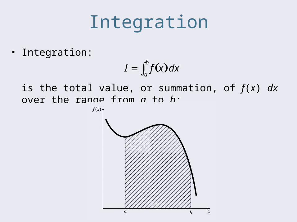
Integration

• Integration:

is the total value, or summation, of f(x) dx over the range from a to b:

I f x a

b dx

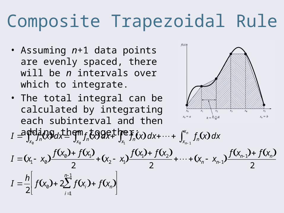
Composite Trapezoidal Rule

• Assuming n+1 data points are evenly spaced, there will be n intervals over which to integrate.

• The total integral can be calculated by integrating each subinterval and then adding them together:

I fn x x0

xn dx fn x x0

x1 dx fn x x1

x2 dx fn x xn 1

xn dx

I x1 x0 f x0 f x1

2 x2 x1

f x1 f x2 2

xn xn1 f xn1 f xn

2

I h

2f x0 2 f xi

i1

n1

f xn

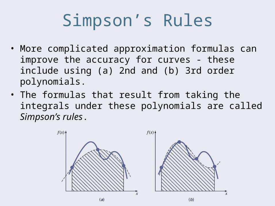
Simpson’s Rules

• More complicated approximation formulas can improve the accuracy for curves - these include using (a) 2nd and (b) 3rd order polynomials.

• The formulas that result from taking the integrals under these polynomials are called Simpson’s rules.

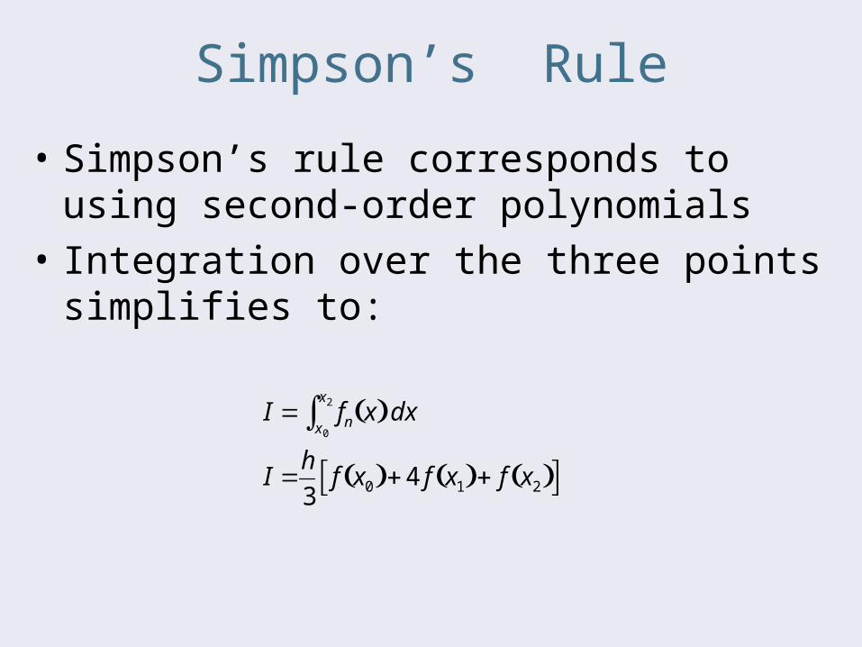
Simpson’s Rule

• Simpson’s rule corresponds to using second-order polynomials

• Integration over the three points simplifies to:

I fn x x0

x2 dx

I h

3f x0 4 f x1 f x2

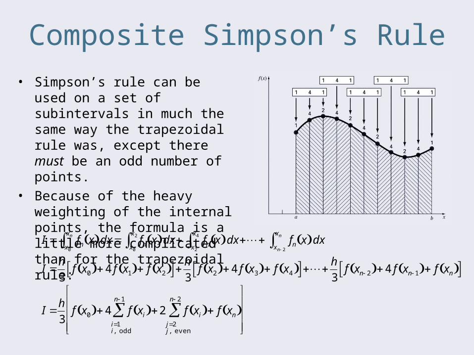
Composite Simpson’s Rule

• Simpson’s rule can be used on a set of subintervals in much the same way the trapezoidal rule was, except there must be an odd number of points.

• Because of the heavy weighting of the internal points, the formula is a little more complicated than for the trapezoidal rule:

I fn x x0

xn dx fn x x0

x2 dx fn x x2

x4 dx fn x xn 2

xn dx

I h

3f x0 4 f x1 f x2 h

3f x2 4 f x3 f x4

h

3f xn 2 4 f xn 1 f xn

I h

3f x0 4 f xi

i1i, odd

n 1

2 f xi j2j , even

n 2

f xn

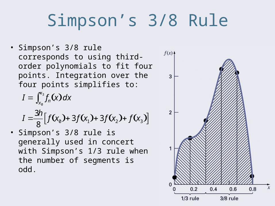
Simpson’s 3/8 Rule

• Simpson’s 3/8 rule corresponds to using third-order polynomials to fit four points. Integration over the four points simplifies to:

• Simpson’s 3/8 rule is generally used in concert with Simpson’s 1/3 rule when the number of segments is odd.

I fn x x0

x3 dx

I 3h

8f x0 3 f x1 3 f x2 f x3

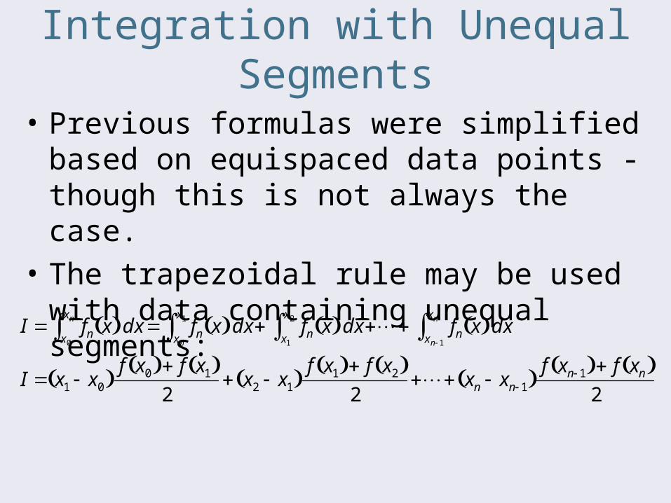
Integration with Unequal Segments

• Previous formulas were simplified based on equispaced data points - though this is not always the case.

• The trapezoidal rule may be used with data containing unequal segments:

I fn x x0

xn dx fn x x0

x1 dx fn x x1

x2 dx fn x xn 1

xn dx

I x1 x0 f x0 f x1 2

x2 x1 f x1 f x2 2

xn xn 1 f xn 1 f xn 2

MATLAB Functions

• MATLAB has built-in functions to evaluate integrals based on the trapezoidal rule

• z = trapz(y)z = trapz(x, y)produces the integral of y with respect to x. If x is omitted, the program assumes h=1.

• z = cumtrapz(y)z = cumtrapz(x, y)produces the cumulative integral of y with respect to x. If x is omitted, the program assumes h=1.

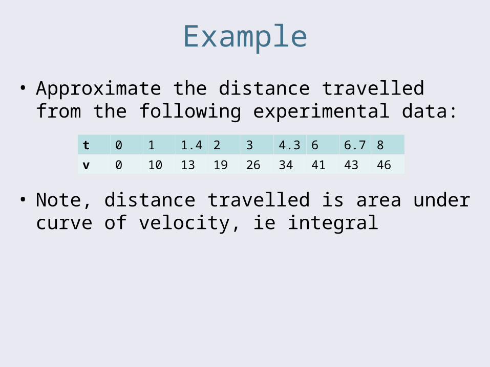
Example

• Approximate the distance travelled from the following experimental data:

• Note, distance travelled is area under curve of velocity, ie integral

t 0 1 1.4 2 3 4.3 6 6.7 8

v 0 10 13 19 26 34 41 43 46

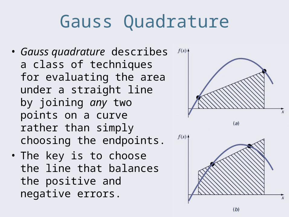
Gauss Quadrature

• Gauss quadrature describes a class of techniques for evaluating the area under a straight line by joining any two points on a curve rather than simply choosing the endpoints.

• The key is to choose the line that balances the positive and negative errors.

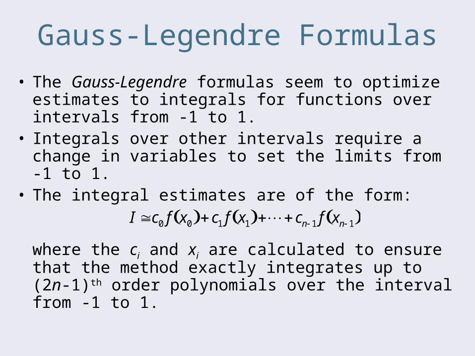
Gauss-Legendre Formulas

• The Gauss-Legendre formulas seem to optimize estimates to integrals for functions over intervals from -1 to 1.

• Integrals over other intervals require a change in variables to set the limits from -1 to 1.

• The integral estimates are of the form:

where the ci and xi are calculated to ensure that the method exactly integrates up to (2n-1)th order polynomials over the interval from -1 to 1.

I c0 f x0 c1 f x1 cn 1 f xn 1

Adaptive Quadrature

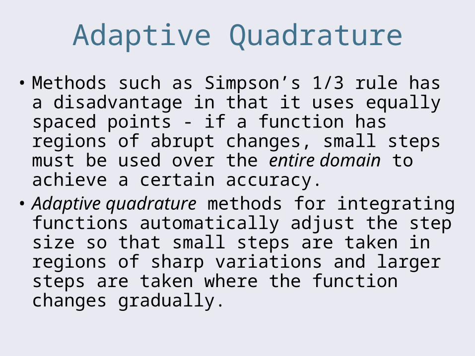
• Methods such as Simpson’s 1/3 rule has a disadvantage in that it uses equally spaced points - if a function has regions of abrupt changes, small steps must be used over the entire domain to achieve a certain accuracy.

• Adaptive quadrature methods for integrating functions automatically adjust the step size so that small steps are taken in regions of sharp variations and larger steps are taken where the function changes gradually.

Adaptive Quadrature in MATLAB

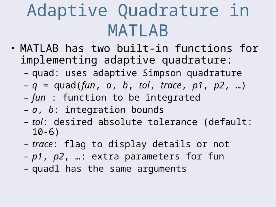
• MATLAB has two built-in functions for implementing adaptive quadrature:– quad: uses adaptive Simpson quadrature– q = quad(fun, a, b, tol, trace, p1, p2, …)– fun : function to be integrated– a, b: integration bounds– tol: desired absolute tolerance (default: 10-6)– trace: flag to display details or not– p1, p2, …: extra parameters for fun– quadl has the same arguments