Embed Size (px)
Citation preview

Scientific computing III 2013: 7. Integration 1
Integration
• A sheet of corrugated roofing is constructed by a machine that presses a flat metallic sheet into one which has a cross section of a sine wave.
- We want to know how much material is needed to construct say 50 cm of corrugated roofing.
- Let’s assume that the profile of the roofing is
.
- We have to find the path length of :
,
- Now we can see that
- Finally we get
xA
f x A 2 x---------sin=
ds
dx
dy
y f x=s f x
s sd
0
s0
=
ds 2 dx 2 dy 2+=
ds dx 2 dy 2+ dx 1 dydx------
2+ dx 1 f x 2+= = =
s dt 1 f t 2+
0
x
dx 1 2 t--------cos2
+
0
x0
= =
Scientific computing III 2013: 7. Integration 2
Integration
- There is no closed form expression for this integral so we have to resort to numerical methods.
- The results using the Romberg method is shown below with values and :
- Just for curiosity: a good approximation for the integral is
A 5 cm= 10 cm=
s x 3.4035 x 0.0703 oscillations+ +=

Scientific computing III 2013: 7. Integration 3
Integration
• Note that quite a lot can be done using the symbolic mathematics programs like Maple, Maxima etc:(example below is made using Maxima from TeXmacs scientific editor; see http://www.math.u-psud.fr/~anh/TeXmacs/TeXmacs.html)
Scientific computing III 2013: 7. Integration 4
Integration
• In this chapter we deal mostly with numerical integration of functions with one variable (1D integrals).
• Multidimensional integrals are more complicated to compute.- A popular method to compute them is the Monte Carlo integration. - Actually, one can show that when the dimension of the problem is larger than 4 then for the MC methods behaves
more nicely than the same quantity for more conventional methods. - Here is the error as a function of the number of function evaluations.
• Numerical integration is sometimes called numerical quadrature.
nfe
nfe
Quadrature \Quad"ra*ture‚ n. [L. quadratura: cf. F. quadrature.]
1. (Math.) The act of squaring; the finding of a square having the same area as some given curvilinear figure; as, the quadrature of a circle; the operation of finding an expression for the area of a figure bounded wholly or in part by a curved line, as by a curve, two ordinates, and the axis of abscissas. [1913 Webster] 2. A quadrate; a square. --Milton. [1913 Webster] 3. (Integral Calculus) The integral used in obtaining the area bounded by a curve; hence, the definite integral of the product of any function of one variable into the differential of that variable. [1913 Webster]

Scientific computing III 2013: 7. Integration 5
Integration
• Our purpose is to compute the value of the integral
- This the area under the curve .
- The general philosophy behind all the numerical integra-tion methods is
1) to approximate the integrand by an
easily integrable function
2) divide the interval into smaller pieces (partition into subintervals)
- The most common approximation is a polynomial.- Easy to integrate.- We already know how to interpolate functions using polynomials.
- Methods differ in 1) the degree of approximation2) the way of partitioning
- As in the case of numerical differentiation there are two directions to gain accuracy:1) refine the partition (decrease step size )2) go to higher degree polynomials
- In fact, the same method — Richardson extrapolation — is used in both integration and differentiation
f x( )
x
a x0= b xN=x1 xN 1–x2
hI f x xd
a
b
=
f x
f x xdab P x xd
ab
f x xdab f x xd
xi 1–
xi
i 1=N=
h
Scientific computing III 2013: 7. Integration 6
Integration: trapezoidal rule
• Let us assume we have an equidistant partition of the interval :
, , ,
- Function values at the nodes are
- The integral is computed as a sum of integrals in the subintervals :
- The most simple (non-trivial) approximation is the linear one:
- In this case the integral of the subinterval is simply the area of the trapezoid
a b
xi x0 ih+= i 0 1 N= x0 a= xN b=
f xi fi
xi xi 1+
I f x xd
xi 1–
xi
i 1=
N=
x1 x2
f1
f2f x fi 1–
fi fi 1––xi xi 1––---------------------- x xi 1––+=
f x( ) xd
x1
x212--- x2 x1– f2 f1+

Scientific computing III 2013: 7. Integration 7
Integration: trapezoidal rule
- And the total integral is
- The error in can be estimated based on what we know about the error in interpolation (let’s use the same notation as
in chapter 6; is now the polynomial order):
for each so that
- Now we have (and )
- The error is (1)
I ITh2--- fi fi 1++
i 0=
Nh fi
i 1=
N 1–h2--- f0 fN++= =
ITn
x a b x a b
f x P x f n xn!
------------------------ x xi–i 1=
n+=
n 2= f x P x– f x2
--------------------- x a– x b–= P x b x– f a x a– f b+b a–
-----------------------------------------------------------=
ET f x P x–
a
bf x
2--------------------- x a– x b–
a
b
= =
Scientific computing III 2013: 7. Integration 8
Integration: trapezoidal rule
- The integral mean-value theorem says that
for which
- This means that we can write (1) as (we removed the explicit depen-dence from ):
- The error term for the integral divided into subintervals is obtained as
,
- For the term in brackets
a b w x f x xd
a
b
f w x xd
a
b
=
x
ETf
2------------- x a– x b–
a
bf
2------------- b a– 3
6-------------------–= =
ETh3
12------– f i
i 1=
Nh3N12
----------– 1N---- f i
i 1=
N= = i xi xi 1–
minx a b f'' x 1N---- f i
i 1=
Nmaxx a b f'' x

Scientific computing III 2013: 7. Integration 9
Integration: trapezoidal rule
- Since is a very nice function (as they always are) its second derivative attains its all values between the minimum and maximum at some point in the interval :
for some value
- So, we finally get the error term in form (and let’s take the absolute value of it)
for some .
- Coding the trapeziodal rule is a piece of cake:
double Trapezoid(double (*f)(double x), double a, double b, int n) {
int i; double h, result;
h = (b-a)/(double)n;result = 0.5*(f(a)+f(b));
for (i=1; i<n; i++) result += f(a+i*h);
return(h*result); }
fa b
f'' 1N---- f i
i 0=
N= a b
ETh3N12
----------f'' h2 b a–12
-----------------------f''= = a b
Scientific computing III 2013: 7. Integration 10
Integration: trapezoidal rule
- For example take the Gaussian on :
For the result is For the result is The correct answer is with seven decimals.
- Let’s estimate the error using the previous expression:
,
It is easy to see that on .
- To have an error of at most we require that or
- Using the routine with n=58 we obtain 0.7468059 which is incorrect in the 5th digit.
- Thus, with the error expression we can estimate how many points we need in order the get the desired accuracy.
- However, this requires that we can estimate the second derivative, which is not always the case.
f x e x– 2= 0 1
N 60= 0.7468071N 500= 0.7468238
0.7468241
f x 2xe x– 2–= f'' x 4x2 2– e x– 2=
f'' x 2 0 1
ETh2
6-----
0.5 4–10 h b a– N 0.01732= N 58

Scientific computing III 2013: 7. Integration 11
Integration: trapezoidal rule
- However, as we look at the formula for the trapezoidal rule
we can see that it is easy to add more points to the expression without the need to redo the computation from the begin-ning:
1) Start with using only the end points and .2) Add more points between the old ones and update accordingly until its value does not change more than a
predetermined value.
IT h fii 1=
N 1–h2--- f0 fN++=
a bIT
N 1=
N 2=
N 4=N 8=
Scientific computing III 2013: 7. Integration 12
Integration: trapezoidal rule
- The formula for the iterated trapezoidal rule is easily derived.
- Let’s assume that the interval is divided into parts:
- We need the method to calculate from :
- The bracketed expression should be calculated with as little extra computation as possible:
a b 2N
IT N h f a ih+i 1=
2N 1–h2--- f a f b++=
IT N IT N 1–
IT N 12---IT N 1– IT N 1
2---IT N 1––+=
IT N h f a ih+i 1=
2N 1–C+=
IT N 1– 2h f a 2ih+i 1=
2N 1– 1–2C+=
C h2--- f a f b+=

Scientific computing III 2013: 7. Integration 13
Integration: trapezoidal rule
- By subtraction we get
- So, the iterative trapezoidal formula is
,
,
IT N 12---IT N 1–– h f a ih+
i 1=
2N 1–h f a 2ih+
i 1=
2N 1– 1–– h f a 2i 1– h+
i 1=
2N 1–
= =
IT N 12---IT N 1– h f a 2i 1– h+
i 1=
2N 1–
+= N 0
h b a–2N
------------= IT 0 12--- b a– f a f b+=
Scientific computing III 2013: 7. Integration 14
Integration: trapezoidal rule
- And in C (notation is a bit different; in anticipation of the Romberg method)
void RecTrapezoid(double (*f)(double x), double a, double b, int N, double *R) {
int i, j, k, kmax=1; double h, sum; h = b-a; /* Value of R(0,0) */ R[0] = (h/2.0)*(f(a)+f(b)); /* Successive approximations R(n,0) */ for (i=1;i<=N; i++) {
h = h/2.0; sum = 0; kmax = kmax*2; for (k=1; k<=kmax-1;k+=2)
sum += f(a+k*h); R[i] = 0.5*R[i-1]+sum*h;
} }

Scientific computing III 2013: 7. Integration 15
Integration: trapezoidal rule
- Example of application
N 9=
Scientific computing III 2013: 7. Integration 16
Integration: higher order methods
• Taking more points into the integral of the subinterval we can develop higher order methods
- Using three points we get the Simpson rule:
- Here we approximate the integrand with a parabola in ;
- This is easily integrated as
f x xdxi 1–
xi
x1 x2 x3
f1f2
f3
x
f x
PN x f x0 x1 xi x xj–j 0=
i 1–
i 0=
N=
f x( ) xd
x1
x3
h 13---f1
43---f2
13--- f3+ + O h5f 4( )+=
x1 x3
f x( ) f2f3 f1–
2h-------------- x x2–
f3 2f2– f1+
2h2----------------------------- x x2– 2 O x2 x– 3( )+ + +=
f x( ) xd
x1
x3
f2f3 f1–
2h-------------- x x2–
f3 2f2– f1+
2h2----------------------------- x x2– 2+ + xd
x1
x3
f2f3 f1–
2h--------------x
f3 2f2– f1+
2h2-----------------------------x2+ + xd
h–
h
=
=

Scientific computing III 2013: 7. Integration 17
Integration: higher order methods
- And by summing the subintegrals such that they do not overlap we get the approximation for the integral
- This formula can not be directly used in iterative computations.
- The error term of the trapezoidal rule can be written in the form (Euler-Maclaurin sum formula; note that here we do not truncate the series after the first term as we did previously):
- Note that we only have even powers of here. are Bernoulli numbers ( , , ...)
- Let’s assume that we have computed the integral using the trapezoidal rule and with subintervals:
- Similarly let be the calculated with subintervals.
- Now if we calculate the weighted average of these two approximations we get
f x( ) xd
x0
xN
h 13---f0
43---f1
23--- f2
43---f3
23--- fN 2–
43---fN 1–
13---fN+ + + + + + +=
f x( ) xd
x0
xN
h 12---f0 f1 f2 fN 1–
12---fN+ + + + +
B2h2
2!------------ f'N f'0–– –
B2kh2k
2k !----------------- fN
2k 1– f02k 1––– –=
h B2k B2 1 6= B4 1 30–=
N SNS2N 2N
S 43---S2N
13---SN–=
Scientific computing III 2013: 7. Integration 18
Integration: higher order methods
- Expanding this we get
- It is easy to see that the error terms with cancel and the lowest order error will be .
- In fact, expanding the above expression we get the Simpson rule.
- Does this sound familiar? It should. What we have is simply Richardson exrapolation (RE).
- We can go further to higher orders by using RE: Romberg algorithm
S 43--- h
h2 f'N f'0–4 12
-----------------------------– O h4+ 13--- h
2---
h2 f'N f'0–12
-----------------------------– O h4––=
h2 O h4

Scientific computing III 2013: 7. Integration 19
Integration: Romberg algorithm
- Richardson extrapolation in short:
1)
2) Goal is to find the limit
3) Choose a value for and calculate the numbers ,
4) Now
5) We can get more accurate estimates by RE using the recursion relation:
6) It can be shown that the quantities have the form
h( ) L a2kh2k
k 1=
–=
L hh 0lim=
h D n 1 h2n-----= n 1 2=
D n 1 L A k 1 h2n-----
2k+=
D n m 1+( ) 4m
4m 1–----------------D n m( ) 1
4m 1–----------------D n 1– m( )–=
D n m
D n m( ) L A k m( ) h2n-----
2k
k m=
+=
D 1 1( )D 2 1( ) D 2 2( )D 3 1( ) D 3 2( ) D 3 3( )
D N 1( ) D N 2( ) D N 3( ) D N N( )
Scientific computing III 2013: 7. Integration 20
Integration: Romberg algorithm
- We have already seen that the trapezoidal formula for the integral has the form similar to we can use RE to improve the estimate of the trapezoidal rule.
- It goes as follows
1) First compute integrals using the trapezoidal rule for different step sizes .
Denote these as .
2) Refine the trapezoidal rule results using RE:
h
h b a–2n
----------------=
R n 0
R n 0 12---R n 1– 0 h f a 2i 1– h+
i 1=
2n 1–
+=
R 0 0 12--- b a– f a f b+=
R n 1 m 1++( ) R n 1 m+( ) 14m 1+ 1–------------------------ R n 1 m+( ) R n m( )–+=

Scientific computing III 2013: 7. Integration 21
Integration: Romberg algorithm
- As a result we get the familiar triangle
- The first column is computed using the trapezoidal rule and others are higher order refinements.
- The recursion formula can be expressed graphically as
R 0 0( )R 1 0( ) R 1 1( )R 2 0( ) R 2 1( ) R 2 2( )
R n 0( ) R n 1( ) R n 2( ) R n n( )
00
20
30
40
10
21
31
41
11
22
32
42
33
43 44
Scientific computing III 2013: 7. Integration 22
Integration: Romberg algorithm
- This is quite simple to code:
void Romberg(double (*f)(double x), double a, double b, int n, double R[][MAXN]) {
int i, j, k, kmax=1; double h, sum;
h = b-a; R[0][0] = (h/2.0)*(f(a)+f(b));
for (i=1; i<=n; i++) {
h = h/2.0; sum = 0; kmax = kmax*2;
/* Trapezoidal estimate R(i,0) */ for (k=1; k<=kmax-1; k+=2)
sum += f(a+k*h); R[i][0] = 0.5*R[i-1][0]+sum*h;
/* Successive R(i,j) */ for(j=1; j<=i; j++)
R[i][j] = R[i][j-1] +(R[i][j-1]-R[i-1][j-1])/(pow(4.0,(double)j)-1.0); }
}
- Here the elements of the array are computed row by row up to the specified number of rows, (this number need not to be very large because the method converges very quickly, e.g., is often suitable).
R i j n
n 4 5=
Scientific computing III 2013: 7. Integration 23
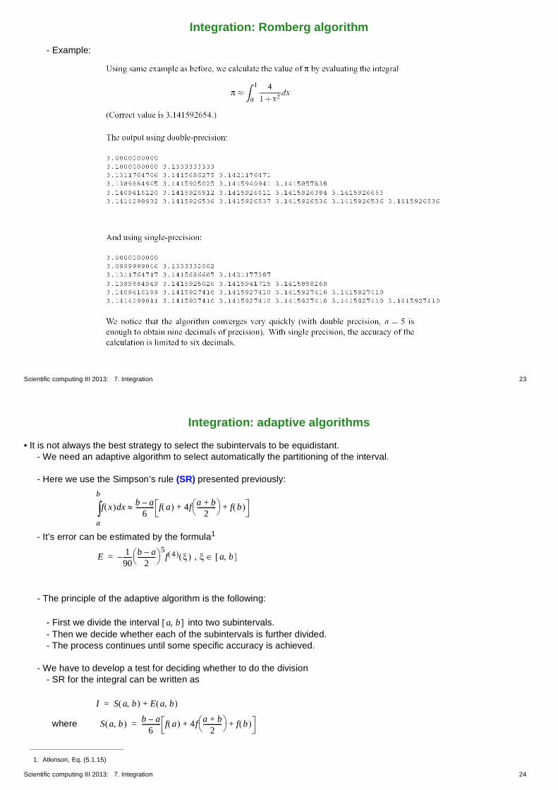
Integration: Romberg algorithm
- Example:
Scientific computing III 2013: 7. Integration 24
Integration: adaptive algorithms
• It is not always the best strategy to select the subintervals to be equidistant.- We need an adaptive algorithm to select automatically the partitioning of the interval.
- Here we use the Simpson’s rule (SR) presented previously:
- It’s error can be estimated by the formula1
,
- The principle of the adaptive algorithm is the following:
- First we divide the interval into two subintervals.- Then we decide whether each of the subintervals is further divided. - The process continues until some specific accuracy is achieved.
- We have to develop a test for deciding whether to do the division- SR for the integral can be written as
where
1. Atkinson, Eq. (5.1.15)
f x xd
a
bb a–
6------------ f a 4f a b+
2------------ f b+ +
E 190------– b a–
2------------
5f 4= a b
a b
I S a b E a b+=
S a b b a–6
------------ f a 4f a b+2
------------ f b+ +=

Scientific computing III 2013: 7. Integration 25
Integration: adaptive algorithms
- Letting we have
, where and
- Two applications of the SR give [ ]
where and
- Now we subtract the first evaluation from the second:
- So the second application of SR can be written as
- This can be used to evaluate the accuracy of our approximation of
h b a–=
I S 1 E 1+= S 1 S a b= E 1 190------ h
2---
5f 4–=
c a b+ 2=
I S 2 E 2+= S 2 S a c S c b+= E 2 190------ h 2
2----------
5f 4– 1
90------ h 2
2----------
5f 4– E 1
16----------= =
I I– 0 S 2 E 2 S 1– E 1–+= =
S 2 S 1– E 2 E 1– 15E 2= =
E 2 S 2 S 1–15
--------------------------=
Well, it is a bit misleading to write the integralin this way. To be precise the errors are allmaximum errors.
EI S 2 E 2+ S 2 S 2 S 1–15
--------------------------+= =
I
Scientific computing III 2013: 7. Integration 26
Integration: adaptive algorithms
- We can use the following test to decide whether to continue the splitting process:
- If the test is not satisfied the interval is split into two subintervals and .
- Performing the test for these subintervals we have to use the tolerance .
115------ S 2 S 1–
a b a c c b
2

Scientific computing III 2013: 7. Integration 27
Integration: adaptive algorithms
- Adaptive algorithm can be programmed as a recursive procedure.
- Two variables are used to calculate the approximation using SR:
one_simpson:
two_simpson:
- After evaluating and we use the division test to check whether to go on with subdivisions.
S 1 S a b h6--- f a 4f c f b+ += =
S 2 S a c S c b+ h12------ f a 4f d 2f c 4f e f b+ + + += =
S 1 S 2 S 2 S 1– 15
Scientific computing III 2013: 7. Integration 28
Integration: adaptive algorithms
- If the criterion is not fulfilled the procedure calls itself with left_simpson corresponding to the left side and the right_simpson corresponding to . At recursive calls .
- Below is the C implementation:
double Simpson(double a, double b, double eps, int level, int level_max) {
int i, j, k, kmax=1; double c, d, e, h, result; double one_simpson, two_simpson; double left_simpson, right_simpson; h = b-a; c = 0.5*(a+b); one_simpson = h*(f(a)+4.0*f(c)+f(b))/6.0; d = 0.5*(a+c); e = 0.5*(c+b); two_simpson = h*(f(a)+4.0*f(d)+2.0*f(c)+4.0*f(e)+f(b))/12.0; /* Check for level */ if (level+1 >= level_max) {
result = two_simpson; printf("Maximum level reached\n");
} else { /* Check for desired accuracy */ if (fabs(two_simpson-one_simpson) < 15.0*eps)
result = two_simpson + (two_simpson-one_simpson)/15.0; /* Divide further */ else {
left_simpson = Simpson(a,c,eps/2.0,level+1,level_max); right_simpson = Simpson(c,b,eps/2.0,level+1,level_max); result = left_simpson + right_simpson;
} } return(result);
}
a cc b 2

Scientific computing III 2013: 7. Integration 29
Integration: adaptive algorithms
Scientific computing III 2013: 7. Integration 30
Integration: adaptive algorithms
- One can explicitely derive higher order integration formulas (so called Newton-Cotes formulas) by increasing the order of the interpolating polynomial.- The first four formulas (including trapezoidal and Simpson’s rules) are as below:
: trapezoidal
: Simpson
: 3/8
: Milne
- Here, as usual, , .
- These are for one subinterval. The composite formulas can be easily derived.- For more information, see e.g. Atkinson, section 5.2.
n 1= f x xd
a
bh2--- f a f b+ h2
12------f 2–=
n 2= f x xd
a
bh3--- f a 4f a b+
2------------ f b+ + h5
90------f 4–=
n 3= f x xd
a
b3h8
------ f a 3f a h+ 3f b h– f b+ + + 3h5
80--------- f 4–=
n 4= f x xd
a
b2h45------ 7f a 32f a h+ 12f a b+
2------------ 32f b h– 7f b+ + + + 8h7
945---------f 6–=
h b a–n
------------= a b
Scientific computing III 2013: 7. Integration 31
Integration: Gaussian quadrature
• In the previous algorithms the integrals were computed by evaluating the function at more or less evenly spaced points and by weighting them appropriately.
• However, the more we have free parameters the higher is the order of the method.
• The basic idea of Gaussian quadrature (GQ) is to choose the points where the function is evaluated in an optimal way.
- This means that the ‘number of degrees of freedom’ is doubled.
- In principle the degree of the method is also doubled: With the same number of function evaluations we get more accu-rate results.
- But remember: The function has to be smooth and nice behaving.
- GQ algorithms are often derived for weighted integrals:
- Here is the weight function. - It is useful for e.g. removing singularities from the integrand.
- The node positions and weights are chosen such that the quadrature is exact for polynomial .
W x( )f x( ) xd
a
b
wjf xj( )j 1=
N
W x
xi wi f x
Scientific computing III 2013: 7. Integration 32
Integration: Gaussian quadrature
- For example in computing the integral
it is wise to choose the weight function as
- The weight function need not be written explicitely: by writing and the integral is
- How do we determine the nodes and weights ?
- A straightforward way is to write down equations that require that the GQ is exact for polynomials upto some degree.
cos2x–exp
1 x2–------------------------------- xd
1–
1
W x( ) 1
1 x2–------------------=
g x( ) W x( )f x( )= vj wj W xj( )=
g x( ) xd
a
b
vjg xj( )j 1=
N=
xi wi

Scientific computing III 2013: 7. Integration 33
Integration: Gaussian quadrature
- Let’s take a simple example:
- Integration in the interval with the weight function .
- We have to determine and such that the error
is zero for polynomials with as high degree as possible.
- Note that the nodes and weights also depend on : , . However, for simplicity, we drop the second subscript.
- We know that
1– 1 W x 1=
f x( ) xd
1–
1
wjf xj( )j 1=
N
xi wi
EN f( ) f x( ) xd
1–
1
wjf xj( )j 1=
N–=
N xj N wj N
EN a0 a1x amxm+ + +( ) a0EN 1( ) a1EN x( ) amEN xm( )+ + +=
Scientific computing III 2013: 7. Integration 34
Integration: Gaussian quadrature
- This means that for all polynomials with degree below only if
,
- Let . We now have two parameters and , which should satisfy
or
- So, the integral takes the form
EN x 0= m 1+
EN xi( ) 0= i 0 1 m=
N 1= x1 w1
EN 1( ) 0=
EN x( ) 0=
1 xd1–
1w1– 0=
x xd
1–
1
w1x1– 0=
w1 2=
x1 0=
f x( ) xd
1–
1
2f 0( )

Scientific computing III 2013: 7. Integration 35
Integration: Gaussian quadrature
- A sidenote: This is actually so called midpoint rule for evaluating the integral:
- Let . Now we have four parameters:
- These are obtained by solving:
,
or
f x( )
x
a x0= b xN=x1 xN 1–x2
h
f x xd
a
b
h fxi 1– xi+
2----------------------
i 1=
N=
N 2= w1 w2 x1 x2
EN xi( ) xi xd
1–
1
w1x1i w2x2
i+– 0= = i 0 1 2 3=
w1 w2+ 2=
w1x1 w2x2+ 0=
w1x12 w2x2
2+ 2 3=
w1x13 w2x2
3+ 0=
Scientific computing III 2013: 7. Integration 36
Integration: Gaussian quadrature
- Solution for this is
and the approximation for the integral is
.
- This rule has a degree of three. Using Simpson’s rule the same accuracy is obtained by using three points.
w1 1=
w2 1=
x13
3-------–=
x23
3-------=
f x( ) xd
1–
1
f 33
-------–( ) f 33
-------( )+

Scientific computing III 2013: 7. Integration 37
Integration: Gaussian quadrature
- For an arbitrary value of we have parameters and they can be obtained requiring that
is accurate for integrals of polynomials with degree or lower.
- The equations are
,
or
- However, this is not the way to go. These are nonlinear equations and not so easy to solve.
- Better methods are based on orthogonal polynomials.
N 2N
f x( ) xd
1–
1
wjf xj( )j 1=
N
2N 1–
EN xi( ) 0= i 0 1 2 2N 1–=
wjxji
j 1=
N 0 i 1 3 5 2N 1–=2
i 1+----------- i 0 2 4 2N 2–=
=
Scientific computing III 2013: 7. Integration 38
Integration: Gaussian quadrature
- Let the integration interval be .
- Inner product of two polynomials (or functions in general) with weight is defined as
.
- Two polynomials are orthogonal if
.
- A polynomial is normalized if
.
- With the following algorithm one can construct a set of mutually orthogonal polynomials with exactly one member of degree , , :
1. ,
2. , (The last term omitted when !)
where , and , .
a b
W x
f g W x f x g x xd
a
b
=
f g 0=
f f 1=
j pj x j 0 1 2=
p 1– x( ) 0 p0 x( ) 1
pj 1+ x( ) x aj– pj x( ) bjpj 1– x( )–= j 0 1 2= j 0=
ajxpj pjpj pj
-----------------= j 0 1 2= bjpj pj
pj 1– pj 1–-----------------------------= j 1 2 3=
Scientific computing III 2013: 7. Integration 39
Integration: Gaussian quadrature
- These polynomials are of the form
- They can always be normalized by dividing by .
- Every polynomial has exactly distinct roots in the interval .
- Roots of interleave the roots of : use to locate roots of .
- The connection between orthogonal polynomials and GQ is the following theorem:
pj x xj cj 1– xj 1– cj 2– xj 2–+ + +=
pj pj
pj x j a b
pj x j 1– pj 1– x pj 1– x pj x
- For each there is a unique numerical integration formula
which is exact for polynomials of . The nodes are the roots of the polynomial which is a member of the set of orthogonal polynomials defined in the interval with respect to weight . The weights are
.
N
W x f x( ) xd
a
b
wjf xj( )j 1=
N
degree 2N 1–pN x
a b W x
wjpN 1– pN 1–
pN 1– xj( )p'N xj( )---------------------------------------=
For proof see e.g. Atkinson chapter 5.3.
Scientific computing III 2013: 7. Integration 40
Integration: Gaussian quadrature
- Note that in principle the weights could be obtained from equations
- Note that when because is a constant and polynomials are orthogonal.
- One can show that with these nodes and weights also polynomials , are integrated exactly.
- Preparing a GQ scheme has three stages
1. Generate the orthogonal polynomials by the recursion formula.2. Determine the roots of the polynomials. 3. Compute the weights.
- List of nodes and weights for the abovementioned ‘classical’ cases can be found in the literature:- See for example Handbook of Mathematical Functions with Formulas, Graphs, and Mathematical Tables,
edited by: Abramowitz, M.; Stegun, I.A(Online version of the book at http://www.knovel.com/knovel2/Toc.jsp?BookID=528 doesn’t seem to include the tables!)
w1p0 x1( ) w2p0 x2( ) w+ Np0 xN( )+ + W x( )p0 x( ) xdab=
w1p1 x1( ) w2p1 x2( ) w+ Np1 xN( )+ + W x( )p1 x( ) xdab=
w1pN 1– x1( ) w2pN 1– x2( ) w+ NpN 1– xN( )+ + W x( )pN 1– x( ) xdab=
W x( )pj x( ) xdab 0= j 0 p0 x
pk x( ) k N N 1 2N 1–+=

Scientific computing III 2013: 7. Integration 41
Integration: Gaussian quadrature
- In the literature there a quite a few ‘classical’ GQ schemes for different weight functions:
Gauss-Legendre:
Gauss-Chebyshev:
Gauss-Laguerre:
Gauss-Hermite:
Gauss-Jacobi: , where
W x( ) 1=1– x 1j 1+ Pj 1+ 2j 1+ xPj jPj 1––=
W x( ) 1
1 x2–------------------=
1– x 1Tj 1+ 2xTj Tj 1––=
W x( ) x e x–=0 x
j 1+ Lj 1+ x– 2j 1+ + + Lj j + Lj 1––=
W x( ) e x2–=– xHj 1+ 2xHj 2jHj 1––=
W x( ) 1 x– 1 x+=1– x 1
cjPj 1+ dj ejx+ Pj fjPj 1––=
cj 2 j 1+ j 1+ + + 2j + +=
dj 2j 1+ + + 2 2–=
ej 2j + + 2j 1+ + + 2j 2+ + +=
fj 2 j + j + 2j 2+ + +=
Scientific computing III 2013: 7. Integration 42
Integration: Gaussian quadrature
- For the Chebyshev GQ the nodes and weights are readily calculated as
- When the nodes and weights are known the integral is computed simply as
- Limits of integration can easily be changed if desired: e.g.
xj
j 12---–
N--------------------cos=
wj N----=
f x( ) xd
a
b
wif xi( )i 1=
N=
1– 1 a b

Scientific computing III 2013: 7. Integration 43
Integration: Gaussian quadrature
- Error estimation of Gaussian quadrature is more complicated than in the case of e.g. trapezoidal or Simpson’s rule.
- For derivation of a general error expression see e.g. Atkinson, chapter 5.3.
- A common practical method to estimate error is the comparison of consecutive iterations (i.e. results with increasing number of nodes):
,
where .
- The fact that in calculating we can not utilize brings some inefficiency here.
- However, there are Gaussian quadrature rules that a designed such that they use the previous nodes.- One example of this is the Gauss-Kronrod quadrature rule.
I In– Im In–
m n
Im In
Scientific computing III 2013: 7. Integration 44
Integration: Gaussian quadrature
- In Gauss-Kronrod quadrature we start from Gaussian quadrature
.
- To get a more accurate estimate we calculate
,
where the nodes of are reused but all weigths and are new.
- In addition there are new nodes .
- Kronrod showed that is accurate for polynomials with degrees up to .
- The error estimate could be calculated as.
- However, experience says that this is usually too pessimistic; a more realistic is.
GN
GN wif xii 1=
N=
K2N 1+ aif xii 1=
Nbjf yj
j 1=
N 1++=
GN ai biN 1+ yjK2N 1+ 3N 1+
GN K2N 1+–
200 GN K2N 1+– 1.5

Scientific computing III 2013: 7. Integration 45
Integration: Gaussian quadrature
- For example the nodes and weights of Gauss-Legendre quadrature:
Scientific computing III 2013: 7. Integration 46
Integration: Gaussian quadrature
- Comparison of the methods (source Atkinson: An Introduction to Numerical Analysis)
I ex xcos xd
0
=

Scientific computing III 2013: 7. Integration 47
Integration: improper integrals
• Improper integrals have one of the following properties:
1) Upper limit is or lower limit is .2) Integrand goes to finite values at the endpoints but can not be evaluated. E.g. at .3) There is an integrable singularity at either endpoint. E.g. at .4) There is an integrable singularity at a known point in the interval.
- Note that some integrals are simply impossible to evalutate: e.g. , .
- In case (1) changing the integration may variable help.
- For the interval suitable substitutions are
:
:
- For interval one can try for example
:
–xsin x x 0=
x 1 2/– x 0=
xdx
-----
1
xcos xd
–
0
t x1 x+------------= 0 0 1
t e x–= 0 1 0
–
t ex 1–ex 1+--------------= – 1– 1
Scientific computing III 2013: 7. Integration 48
Integration: improper integrals
- Gauss-Laguerre and Gauss-Hermite quadratures are defined for infinite intervals:
Gauss-Laguerre:
Gauss-Hermite:
- For example can be computed by using Gauss-Laguerre
quadrature ( ):
- Results for various values of (exact value ):
2 0.432459454679844 4 0.504879279460199 8 0.499987753735300 16 0.499999999985333 32 0.500000000000000 64 0.500000000000000 128 0.500000000000000 256 0.500000000000000
W x( ) x e x–=0 x
W x( ) e x2–=– x
I e x– xsin xd
0
=
0=
I wi xisini 1=
N
N I 12---=

Scientific computing III 2013: 7. Integration 49
Integration: improper integrals
- Case (2) can often be computed by open methods (i.e. methods that do not evaluate the function at the end points).
- Note that GQs are examples of these kind of rules.
- Case (3) can often be computed by changing the variable.
- A simple case: . Its exact value is .
- Applying Gauss-Laguerre quadrature (with the proper interval scaling enables us to compute : 2 1.65068012388578 4 1.80634254040352 8 1.89754094923051 16 1.94722751142287 32 1.97320909141769 64 1.98650087152911128 1.99322419413980256 1.99660549565866512 1.99830109231141
- However, convergence is slow even though GLQ removed the difficulty of eveluating the function in origin.
- In general for inverse-square-root singularities in the integral the following substitution may help:
I xdx
------
0
1
= I 2=
0 1 1– 1 I
f x xd
a
b
x a– t2=
Scientific computing III 2013: 7. Integration 50
Integration: improper integrals
- This gives the integral in the form
- Now our example integral reduces to ( , , )
.
- Case (4) can be integrated in two parts so that we end up with singularities at the endpoints.
f x xd
a
b
2tf a t2+ td
0
b a–
=
a 0= b 1= f x x 1 2/–=
xdx
------
0
1
2tf t2 td
0
1
2 td
0
1
2= = =

Scientific computing III 2013: 7. Integration 51
Integration: summary of 1D integrals
• If your function is one of those nice-behaving ones Gaussian quadrature is probably the best choice.- You need to know the nodes and weights.- They can be found in the literature (in form of tables and subroutines) for ‘classical’ quadrature weights. - Also, when going to higher number of nodes the previous results can not be utlilized.
• Romberg’s method is almost as good as GQ. - For nice functions if you don’t know suitable GQ rules.
• If your function is not nice-behaving trapezoidal or Simpson’s rule are robust though slow.- Adaptive algorithms may save some CPU time.
Scientific computing III 2013: 7. Integration 52
Integration: multidimensional integrals
• Multidimensional integrals are problematic for two reasons:
1) The number of function evaluations increases quickly when the desired accuracy becomes better.
2) Integration volume may have a complicated shape.
• Certain integrals can be reduced to 1D.• For example so called iterated integrals can be expressed as 1D integrals:
• If the integration volume is complicated but the function smooth one could use the Monte Carlo method.
• If the volume is simple and the function smooth we can break up the integral into repeated 1D integrals:
tnd
0
x
tn 1–d
0
tn
t2d
0
t3
f t1( ) t1d
0
t21
n 1– !------------------ x t– n 1– f t( ) td
0
x
=
I xd yd xf x y z( )d
x y zf x y z( )d
z1 x y( )
z2 x y( )
d
y1 x( )
y2 x( )
d
x1
x2
=
=

Scientific computing III 2013: 7. Integration 53
Integration: multidimensional integrals
- E.g. integration of a function over unit circle:
- Let’s call the innermost integral in the above equation as
and its integral as
- The final results is the integral of over
xd
1–
1
yd f x y( )
1 x2––
1 x2–
G x y
G x y( ) zf x y z( )d
z1 x y( )
z2 x y( )
=
H x
H x( ) G x y( ) yd
y1 x( )
y2 x( )
=
H x1 x2
I H x( ) xd
x1
x2
=
Scientific computing III 2013: 7. Integration 54
Integration: multidimensional integrals
- Graphically:
oute
rmos
t int
egra
l
innermost integral
y
x

Scientific computing III 2013: 7. Integration 55
Integration: multidimensional integrals
- In C we could say it as below static double xsav,ysav;static double (*nrfunc)(double,double,double);
double quad3d(double (*func)(double, double, double), double x1, double x2){
double qgaus(double (*func)(double), double a, double b);
double f1(double x);
nrfunc=func;return qgaus(f1,x1,x2);
}
double f1(double x){
double qgaus(double (*func)(double), double a, double b);
double f2(double y);double yy1(double),yy2(double);
xsav=x;return qgaus(f2,yy1(x),yy2(x));
}
double f2(double y){
double qgaus(double (*func)(double), double a, double b);double f3(double z);double z1(double,double),z2(double,double);ysav=y;return qgaus(f3,z1(xsav,y),z2(xsav,y));
}
double qgaus(double (*func)(double), double a, doubleb){
int j;double xr,xm,dx,s;static double x[]={0.0,0.1488743389,0.4333953941,
0.6794095682,0.8650633666,0.9739065285};static double w[]={0.0,0.2955242247,0.2692667193,
0.2190863625,0.1494513491,0.0666713443};xm=0.5*(b+a);xr=0.5*(b-a);s=0;for (j=1;j<=5;j++) {
dx=xr*x[j];s += w[j]*((*func)(xm+dx)+(*func)(xm-dx));
}return s *= xr;
}
double f3(double z){return (*nrfunc)(xsav,ysav,z);
}
Scientific computing III 2013: 7. Integration 56
Integration: multidimensional integrals
- And below the main program using this routine:
/* Driver for routine quad3d */#include <stdio.h>#include <math.h>#define PI 3.1415927#define NVAL 10static double xmax;double quad3d(double (*func)(double, double, double), double x1, double x2);double func(double x,double y,double z){
return x*x+y*y+z*z;}double z1(double x,double y){
return (double) -sqrt(xmax*xmax-x*x-y*y);
}double z2(double x,double y){ return (double) sqrt(xmax*xmax-x*x-y*y);}double yy1(double x){
return (double) -sqrt(xmax*xmax-x*x);}double yy2(double x){
return (double) sqrt(xmax*xmax-x*x);}
int main(void){int i;double xmin,s;
printf(“Integral of r^2 over a spherical volume\n\n”);printf(“%13s %10s %11s\n”,”radius”,”QUAD3D”,”Actual”);for (i=1;i<=NVAL;i++) {
xmax=0.1*i;xmin = -xmax;s=quad3d(func,xmin,xmax);printf(“%12.2f %12.6f %11.6f\n”,xmax,s,4.0*PI*pow(xmax,5.0)/5.0);
}return 0;}

Scientific computing III 2013: 7. Integration 57
Integration: multidimensional integrals
- This program integrates ( ) over a sphere with radius .
- The exact value is .
- And the results:
3dint> a.outIntegral of r^2 over a spherical volume
radius QUAD3D Actual 0.10 0.000025 0.000025 0.20 0.000805 0.000804 0.30 0.006112 0.006107 0.40 0.025756 0.025736 0.50 0.078601 0.078540 0.60 0.195583 0.195432 0.70 0.422733 0.422406 0.80 0.824187 0.823550 0.90 1.485211 1.484063 1.00 2.515219 2.513274
- Note the large error though we use a 10-point GQ in 1D integration.
f x y z r2= r x2 y2 z2+ += R45--- R5
Scientific computing III 2013: 7. Integration 58
Integration: multidimensional integrals
• Another way to compute multidimensional integrals is so called product rule
- Let’s assume that we have a 2D integral
- As in the 1D case we could try to find an approximation of the form
which integrates exactly 2D polynomials with degree no more than . - is the error.
- A 2D polynomial with degree has terms and .- For example when the polynomial is
- One (though not necessarily the optimal) way is so called product rule.
I f x y( ) AdD
=
I wif xi yi( )i 1=
NRN+=
dRN
d xpyq p q+ dd 2=
a00 a10x a01y a20x2 a11xy a02y2+ + + + +

Scientific computing III 2013: 7. Integration 59
Integration: multidimensional integrals
- Let’s write
(1)
(2)
- This 2D integral can be written in the form
f x( ) xd wif xi( )i 1=
NR1+=
g y( ) yd
a
b
pig yi( )i 1=
MR2+=
f x y( ) xd yd
a
b
wif xi y( )i 1=
NR1+ yd
a
b
wi f xi y( ) yd
a
b
i 1=
NR1 yd
a
b
+
wi pjf xi yj( )j 1=
MR2+
i 1=
NR1 yd
a
b
+
wipjf xi yj( )j 1=
M
i 1=
NwiR2
i 1=
NR1 yd
a
b
+ +
wipjf xi yj( )j 1=
M
i 1=
NR+
=
=
=
=
=
Scientific computing III 2013: 7. Integration 60
Integration: multidimensional integrals
- This the product rule.
- We use points to compute the integral.
- Below is a simple example of a product rule:
- One can show that if equations (1) and (2) are exact for polynomials with degrees no more than and then product
rule integrates exactly polynomials where and .
NM
3 2
1 1
1– 1–
d1 d2
xpyq p d1 q d2

Scientific computing III 2013: 7. Integration 61
Integration: multidimensional integrals
- Let’s take an example:
- Exact value of the integral
- The code on the following page computes this integral with number of nodes as an input.
- Note: This code uses NR routines; e.g. gauleg to compute Gauss-Legendre nodes and weights.
f x y( ) xye x2y–=x y 0 1
f x y xd yd
0
1
0
1
xye x2y– xd yd
0
1
0
11
2e------ 0.18393972= =
Scientific computing III 2013: 7. Integration 62
Integration: multidimensional integrals
#include <stdio.h>#include <math.h>#include <stdlib.h>#define NRANSI#include “nr.h”#include “nrutil.h”
float f(float x, float y){ return x*y*exp(-x*x*y); /* return sin(5.0*x*x)*cos(y*x); */
}
int main(int argc, char **argv){ int nx,ny,i,j; float x1,x2,y1,y2; float s; float *xx,*wx,*xy,*wy;
if (argc!=7 ) { fprintf(stderr,”Komentorivi: %s nx ny x1 x2 y1 y2\n”,argv[0]); return (1);
} nx=atoi(*++argv); ny=atoi(*++argv); x1=atof(*++argv); x2=atof(*++argv); y1=atof(*++argv); y2=atof(*++argv);
xx=vector(1,nx); wx=vector(1,nx); xy=vector(1,ny); wy=vector(1,ny);
gauleg(x1,x2,xx,wx,nx);
gauleg(y1,y2,xy,wy,ny); s=0.0; for (i=1;i<=nx;i++) for (j=1;j<=ny;j++)
s+=wx[i]*wy[j]*f(xx[i],xy[j]); printf(“GL-kvadratuuri %20.12g\n”,s); return (0);}#undef NRANSI

Scientific computing III 2013: 7. Integration 63
Integration: multidimensional integrals
- Results:
2d> xgauleg 3 3 0 1 0 1GL-kvadratuuri 0.183959037066Tarkka arvo 0.1839397251612d> xgauleg 5 5 0 1 0 1GL-kvadratuuri 0.183939725161Tarkka arvo 0.183939725161
- This is not bad. Though note that the function is smooth and the integration volume regular.- Not also that the function is evaluated nx ny times.
- A more difficult case is
- Because the integral oscillates we need many nodes to get reason-able results:
I 5x2sin xy ydcos xd
0
3
0
3
=
Scientific computing III 2013: 7. Integration 64
Integration: multidimensional integrals
- Sometimes the integration area is not rectangular.
- By suitably changing variables the are can be transformed into rectangular shape:- E.g. integral over a triangle:
,
- Let’s change variables: , ,
- Now the integral is written as
and we can use the product rule.
- However, the transformation changes the sampling density of the integration area:
I f x y( ) Ad= x y : 0 x 1 0 y x=
u x= v yx--= du dx= dv dy
x------=
I xd
0
1
yd f x y( )
0
x
ud
0
1
vd f x y( )u
0
1
= =

Scientific computing III 2013: 7. Integration 65
Integration: multidimensional integrals
- There are methods where the nodes are chosen in a more optimal way than in the prod-uct rule.
- For example the 3x3 Gauss-Legendre product rule has degree of 5 and need 9 function evaluations:
- Radon formula gives more optimal nodes: in the 7 point method
where , , .
- This method is of degree 5 and needs only 7 function evaluations.
f x y( ) xd yd
1–
1
1–
159--- f r s( ) f r s–( ) f r– s( ) f r– s–( )+ + +
2063------ f 0 t( ) f 0 t–( )+ 8
7---f 0 0( )+ +
r 3 5= s 1 3= t 14 15=
Scientific computing III 2013: 7. Integration 66
Integration: multidimensional integrals
• Monte Carlo (MC) method
- Computing the value of by MC:
- Generate random numbers in the interval and calculate the number of hits
to the gray area :
- The accuracy of the result depends on and behaves as :
1 A
BC
O x
y
Ntot 0 1
Nhit
4NhitNtot
-------------
Ntot O Ntot1– 2

Scientific computing III 2013: 7. Integration 67
Integration: multidimensional integrals
- In 1D integration other methods are superior compared to MC.
- But let’s take an example from statistical physics:
- We have to compute the average potential energy of the system
where and is the system potential energy.
- Our system consists of 100 atoms in a box .
- A rough Simpson’s method would need function evaluations.
- MC integration using unbiased sampling:
1) Generate configuration by randomly placing atoms to the box.
2) Calculate system potential energy and Boltzmann factor
- The integral becomes now
U Ue U– rd=
1 kBT= U
x y z L 2– L 2
10300
i
U i e U–
U U i e U i–
i 1=
n
Scientific computing III 2013: 7. Integration 68
Integration: multidimensional integrals
- This is very inefficient as can be seen from the figures below:
- Here the Metropolis sampling was started from a random gonfiguration; .
- The interaction was Lennard-Jones:
unbiased
T 5 K=
U r( ) 4r---
12
r---
6–=

Scientific computing III 2013: 7. Integration 69
Integration: multidimensional integrals
- So, when generating the points in MC integration it is useful to do that in such a way that we sample the volume in those places where the integrand is not negligible: importance sampling.
- Assume we must compute the integral
- Let’s write it in the form
where is an arbitrary probability density (i.e. , ).
- Now we generate a sample of size by choosing random numbers that have the distribution in the interval .
- In this case the integral can be written as
F xf x( )d
x1
x2
=
F x f x( )x( )
--------- x( )d
x1
x2
=
x x( ) 0 x x( )dx1
x2 1=
N xx1 x2
F f( )( )
----------=
Scientific computing III 2013: 7. Integration 70
Integration: multidimensional integrals
- The most simple density would be
,
when the integral would be
- What would be the optimal density function?
- The error of the integral can be written as
- As an integral this is
x( ) 1x2 x1–----------------= x1 x x2
Fx2 x1–
N---------------- f i( )
i 1=
N
F 2 f2 2 f 2–=
F 2 f22
------ xd
x1
x2f--- xd
x1
x2 2
– f22
------ xd
x1
x2
f xd
x1
x2 2
–= =

Scientific computing III 2013: 7. Integration 71
Integration: multidimensional integrals
- Now we apply variational calculus to find the optimal :
(Note the additional condition of normalization of .)
- By dropping the middle term (it doesn’t depend on ) and moving the variation inside the integral we get
- Really nice: in order to get we should know the integral of the function (well, of its absolute value)!
- There are workarouns to this problem:
1) need not necessarily be exactly the optimum but being near to it may suffice.2) Generating samples from a distribution can be done without knowing its normalization.
Markov chain Monte Carlo
------ f22
------ xd
x1
x2
f xd
x1
x2 2
– xd
x1
x2
+ 0=
f2
2------– + 0= f
f xdx1
x2------------------=
Scientific computing III 2013: 7. Integration 72
Integration: multidimensional integrals
- In Metropolis MC we generate a series of points (or system states or configurations) in such a way that they obey the desired probability density. (Markov chain)
- The algorithm consists of the probability density of the states : , and the transition probabilites between states: .
- The series of states generated by these obey the probability density if
(i)
(ii)
(iii)
- The system also has to be ergodic: it is possible to go from a state to any other state (not in one step necessarily).
- What is essential here is that only the ratio of probability densities is needed no need to know the normalization.
- Conditions (i)-(iii) are not very strict: They leave a lot for your imagination.
m m mn
m
mn 0
mnn
1=
m mn n nm=

Scientific computing III 2013: 7. Integration 73
Integration: multidimensional integrals
- Metropolis Monte Carlo is one (and the first1) realization of this
- Here is a symmetric stochastic matrix: . In a way it describes the ‘trial’ probability of the.
- Based on the symmetry of one can easily show that the above algorithm obeys the conditions (i),(ii),(iii).
- If you want to know more about the MC method attend the course(s)
Basics of Monte Carlo simulationsMonte Carlo simulations in physicshttp://beam.helsinki.fi/~eholmstr/mc/
1. N. Metropolis, A. W. Rosenbluth, M. N. Rosenbluth, A. H. Teller, E. Teller, Equation of State Calculations by Fast Computing Machines, J. Chem. Phys., 21 (1953) 1087.
mn
mn n m m n;
mnn
m------- n m m n,;
1 mnm n
– m n=
=
mn mn nm=
Scientific computing III 2013: 7. Integration 74
Integration: multidimensional integrals
• A final note: A list of top ten algorithms (one of them) of the 20th century can be found at http://www.siam.org/siamnews/05-00/current.htm
- Below is the list (it seems to be in the cronological order)
1. Metropolis Monte Carlo. von Neuman et al., 1946
2. Simplex linear programming method (optimization). Dantzig, 1947
3. Krylov subspace iteration method (solving for large matrices). Hestenes et al., 1950
4. Decompositional approach to matrix computations. Householder, 1951
5. Fortran optimizing compiler. Backus, 1957
6. QR algorithm for eigenvalue problems. Francis, 1959-61
7. Quicksort. Hoare, 1962
8. Fast Fourier transform. Cooley and Tukey, 1965
9. Integer relation detection algorithm. Ferguson and Forcade, 1977
10. Fast multipole algorithm. Greengard and Rokhlin, 1987
Ax b=

Scientific computing III 2013: 7. Integration 75
Integration: practical tools
• Matlab quad adaptive Simpsonquadl adaptive Lobatto (GQ on with
and end points included)
• Octavequad integration using Quadpack routines
• QuadpackPackage of integration routines written in Fortran 77. Atkinson: ‘The package is well tested and appears to be an excellent collection of programs.’Can be downloaded from http://www.netlib.org/quadpackSee also http://www.scs.fsu.edu/~burkardt/f_src/quadpack/quadpack.html
• SLATECBoth adaptive and non-adaptive routines(d)gaus8:adaptive 8-point Gauss-Legendre (d)qnc79:adaptive 7-point Newton-Cotes
• GSLReimplements the algorithms used in QuadpackBoth adaptive and non-adaptive routines
Adaptive Gauss: use previous nodes (butnew weights) (Kronrod extension; Gauss-Kronrod quadrature):
Patterson: points.
W x f x xd
a
b
wif xii 0=
N=
W x f x xd
a
b
vif xii 0=
2N 1+=
N N M+
Note:-point Newton-Cotes =
approximating the functionby a polynomial of degree
Trapezoidal rule = 2-point Newton-CotesSimpson = 3-point Newton-Cotes
N
N 1–
1– 1 W x 1=
Scientific computing III 2013: 7. Integration 76
Integration: practical tools
• In many applications there are certain special integrals for which efficient methods have been developed.
- Double-folded integrals using Fourier-Bessel expansion.- Fermi-Dirac integrals.- Fourier integrals.


![7. Random walks - Acclab h55.it.helsinki.fiknordlun/mc/mc7nc.pdf7.2. Simple random walks and diffusion [G+T 7.3] 7.2.1. One-dimensional walk Let us first consider the simplest possible](https://img.dokumen.tips/doc/110x75/5ae6a85e7f8b9a9e5d8dfd62/7-random-walks-acclab-h55it-knordlunmcmc7ncpdf72-simple-random-walks-and.jpg)


